intro to comp genomics lecture 11: using models for sequence evolution
Post on 22-Dec-2015
222 views
TRANSCRIPT

Intro to Comp Genomics
Lecture 11: Using models for sequence evolution

Comparing everything
Our intuition:
Feature X similar among a group of species -> Feature X is important
Feature X can be:
• Sequence• Gene expression (human brain vs chimp brain?)• Genic structure (Exon/intron)• Protein complexes • Protein networks• TF-DNA interaction
Two main difficulties:
Species have common ancestry – a lot of stuff may be similar just because it did not diverge yet
Species are related through phylogenetic trees – similarity should be following a tree structure

Modeling multiple genome sequences
Genome1
Genome2
AGCAACAAGTAAGGGAAACTACCCAGAAAA….AGCCACATGTAACGGTAATAACGCAGAAAA….AGCAACAAGAAAGGGTTACTACGCAGAAAA….
Alignment
Statistics
Genome3
ACGT
A C G T
AC
GT
s
s
s s
sMarkov process
Markov process
Unobserved ancestral
Unobserved ancestral

Tree models
H2
S3
S2 S1
H1
For a locus j:
Extant Species Sj1,..,n
Ancestral species Hj1,..(n-1)
Tree T: Parents relation pa Si , pa Hi
(pa S1 = H1 ,pa S3 = H2
The root: H2)
Val(X) = {A,C,G,T}
An evolutionary model = a joint distribution Pr(h,s)
Locus independence: ),Pr(),Pr( jjj hshs

Tree models
ATree: T, Species S1,..,n
Parents relation pa Si
Markov assumption still in effect..but branching complicates it
C
CC
A
ii paxxiii Qtxx ,)exp()pa|Pr(
)Pr( rooth
We need a little more:
)pa|Pr()Pr(),Pr( ! iirootiroot xxhhs
The model:
)|Pr()|Pr()|Pr()|Pr()Pr()Pr( 111223212 hshshshhhs In the triplet:

Tree models
Toy model:
Triplet phylogeny
Substitution probability on all of the branches:
96.001.002.001.0
01.096.001.002.0
02.001.096.001.0
01.002.001.096.0
)|Pr( yx
Uniform background probability: P(x) = 0.25
H2
S3
S2 S1
H1

Tree models
Marginal probability of Xi (any r.v.) :
ii xXsh
iii shPxXx|,
),()Pr()Pr(
)|Pr(/),(),|Pr(|
sshPsxhxhh
i
i
Given partial observations s:
“ancestral inference”
h
shPs )|,()|Pr(
The Total probability of the data:
likelihood of the model given the data
H2
S3
S2 S1
H1

Tree models
?
A
C A
?
xhh
i
i
shPsxh|
),()|Pr(
Given partial observations s:
)),,Pr(( ACA
The Total probability of the data:
)),,(|Pr( 1 ACAAh
?
?
96.001.002.001.0
01.096.001.002.0
02.001.096.001.0
01.002.001.096.0
)|Pr( yx

Intuition – maximum parsimony
?
A
C A
?
“Parsimony” ~ minimal change
The “small” parsimony problem: Find ancestral sequences that minimize the number of substitutions along the tree branches
What is the minimal number of substitutions?
(All branches are equal, all substitutions are equal)
(The “big” parsimony problem: Find the tree topology that gives minimal parsimony score given a set of loci)
C
C 2 substitutions
A
A 1 substitution

Algorithm (Following Fitch 1971):
Up(i):if(extant) { up_set[i] = Si; return}up(right(i)), up(left(i))up_set[i] = up_set[right[i]] ∩ up_set[left[i]]if(up_set[i] = 0)
D += 1 up_set[i] = up_set[right[i]] + up_set[left[i]]
Down(i):down_set[i] = up_set[sibling[i]] ∩ down_set[par(i)]if(down_set[i] = 0) {
down_set[i] = up_set[sibling[i]] + down_set[par(i)]}
Algorithm:D=0up(root);down_set[root] = 0;down(right(root));down(left(root));
Intuition – maximum parsimony?
S3
S2 S1
? up_set[4]
up_set[5]

Algorithm (Following Fitch 1971):
Up(i):if(extant) { up_set[i] = Si; return}up(right(i)), up(left(i))up_set[i] = up_set[right[i]] ∩ up_set[left[i]]if(up_set[i] = 0)
D += 1 up_set[i] = up_set[right[i]] + up_set[left[i]]
Down(i):down_set[i] = up_set[sib[i]] ∩ down_set[par(i)]if(down_set[i] = 0) {
down_set[i] = up_set[i]}down(left(i)), down(right(i))
Algorithm:D=0up(root);down_set[root] = 0;down(right(root));down(left(root));
Intuition – maximum parsimony?
S3
S2 S1
? down_set[4]
down_set[5]
up_set[3]
Set[i] = up_set[i] ∩ down_set[i]

Algorithm (Following Felsenstein 1981):
Up(i):if(extant) { up[i][a] = (a==Si ? 1: 0); return}up(r(i)), up(l(i))iter on a
up[i][a] = b,c Pr(Xl(i)=b|Xi=a) up[l(i)][b] Pr(Xr(i)=c|Xi=a) up[r(i)][c]
Down(i):
down[i][a]= b,c Pr(Xsib(i)=b|Xpar(i)=c) up[sib(i)][b] Pr(Xi=a|Xpar(i)=c) down[par(i)][c]
down(r(i)), down(l(i))Algorithm:
up(root);LL = 0;foreach a {
L += log(Pr(root=a)up[root][a])down[root][a]=Pr(root=a)
}down(r(root));down(l(root));
Probabilistic inference?
S3
S2 S1
? up[4]
up[5]
Felsentstein

Algorithm (Following Felsenstein 1981):
Up(i):if(extant) { up[i][a] = (a==Si ? 1: 0); return}up(r(i)), up(l(i))iter on a
up[i][a] = b,c Pr(Xl(i)=b|Xi=a) up[l(i)][b] Pr(Xr(i)=c|Xi=a) up[r(i)][c]
Down(i):
down[i][a]= b,c Pr(Xsib(i)=b|Xpar(i)=c) up[sib(i)][b] Pr(Xi=a|Xpar(i)=c) down[par(i)][c]
down(r(i)), down(l(i))Algorithm:
up(root);LL = 0;foreach a {
L += log(Pr(root=a)up[root][a])down[root][a]=Pr(root=a)
}down(r(root));down(l(root));
?
S3
S2 S1
? down[4]
down5]
up[3]
P(hi|s) = up[i][c]*down[i][c]/
(jup[i][j]down[i][j])
Probabilistic inference
Felsentstein

Inference as message passing
s
s
s s
s
s
sYou are P(H|our data)
You are P(H|our data)
I am P(H|all data)
DATA

Inference as message passing
A CC
C
DATA
96.001.002.001.0
01.096.001.002.0
02.001.096.001.0
01.002.001.096.0
)|Pr( yx
Up:(0.01)2,(0.96)2,(0.01)2,(0.02)2
Down:(0.25),(0.25),(0.25),(0.25)
Up:(0.01)(0.96),(0.01)0.96),(0.01)(0.02),(0.02)(0.01)

Learning: Branch decomposition
3
2 1
5
4
5
3
5
4
1
4
2
4
Can we learn each branch independently?
We know how to compute the ML model given two observed species
We have P(S|D) for each species, can we substitute it for the statistics:
))),|(),|(((maxarg )( sXEsXEL ipai
A G C TAGCT
loci
ipaiii sXPsXPXXE ),|(),|()( )(pa
)|Pr(maxarg)|(maxarg DDL

Transition posteriors: not independent!
A CA
C
DATA
96.001.002.001.0
01.096.001.002.0
02.001.096.001.0
01.002.001.096.0
)|Pr( yxDown:(0.25),(0.25),(0.25),(0.25)
Up:(0.01)(0.96),(0.01)0.96),(0.01)(0.02),(0.02)(0.01)
Up:(0.01)(0.96),(0.01)0.96),(0.01)(0.02),(0.02)(0.01)

Learning: Second attempt
3
2 1
5
4 5
3
5
4
1
4
2
4
Can we learn each branch independently?
Given P(Spai->Si|D) for each species, can we substitute it for the statistics?
)),|((maxarg
)|Pr()|Pr(sib
]][[]][[pa]][[sib1
)|,(
)(
)()(
)(
iiipa
ipaiipai
loci ciii
iipa
DXXEL
aXbXaXcX
bXupaXdowncXupZ
SbXaXE
i

Expectation-Maximization
3
2 1
5
4 5
3
5
4
1
4
2
4
)),|((maxarg )(1
iiipaki SXXELL
i
)|Pr()|Pr(sib
]][[]][[pa]][[sib1
)|,(
)()(
)(
aXbXaXcX
bXupaXdowncXupZ
SbXaXE
ipaiipai
loci ciii
iipa
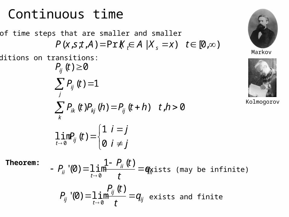
Continuous time
),0[)|Pr(),;,( txXAXAtsxP st
ji
jitP
hthtPhPtP
tP
tP
ijt
ijk
kjik
jij
ij
0
1)(lim
0,)()()(
1)(
0)(
0
Conditions on transitions:
Theorem:
ijij
tij
iiii
tii
qt
tPP
qt
tPP
)(lim)0('
)(1lim)0('
0
0exists (may be infinite)
exists and finite
Think of time steps that are smaller and smaller
Markov
Kolmogorov

Rates and transition probabilitiesThe process’s rate matrix:
nininnn
ni
i
ni
i
qqqq
qqqq
qqqq
Q
..
..........
..........
..
..
210
1121110
0020100
Transitions differential equations (backward form):
)(]1)([)()(
)()()()()(
tPsPtPsP
tPtPsPtPtsP
ijiiik
kjik
ijk
kjikijij
)()()('0 tPqtPqtPs ijiiik
kjikij
)exp()()()(' QttPtQPtP

Matrix exponentialThe differential equation:
)exp()()()(' QttPtQPtP
Series solution:
)exp(!
1
!))'(exp(
!
1)exp(
0
1
0
0
QtQtQi
QtQi
iQt
tQi
Qt
i
i
ii
i
i
i
i
i
1-path 2-path 3-path 4-path 5-path
Summing over different path lengths:

Computing the matrix exponential
t
t
t
ii
i
i
i
i
i
i
i
ne
e
e
t
tti
ti
Q
tQi
Qt
00
00
00
)exp(
)exp()!
1()(
!
1
!
1)exp(
2
1
00
0

Computing the matrix exponential
i
i
itQi
Qt
0 !
1)exp(
Series methods: just take the first k summandsreasonable when ||A||<=1if the terms are converging, you are ok
can do scaling/squaring:
Eigenvalues/decomposition:good when the matrix is symmetricproblems when having similar eigenvalues
Multiple methods with other types of B (e.g., triangular)
m
m
QQ ee
0!
1iQ
i
1SSeB

Learning a rate matrix
3
2 1
5
4 5
3
5
4
1
4
2
4
What if we wish to learn a single rate matrix Q?
)exp()Pr( )( iiipa QtXX
,..),,|Pr(maxarg 21,..,, 121ttQs
nttQ
Learning is easy for a single, fixed length branch. Given (inferred) statistics nk for multiple branch lengths, we must optimize a non linear likelihood function
kijn
ijkjik QttQsL ))(exp(),|( ,,

Learning: Sharing the rate matrix
3
2 1
5
4 5
3
5
4
1
4
2
4
kijn
ijkjik QttQsL ))(exp(),|( ,,
Use generic optimization methods: (BFGS)
?))log(exp(
?),|(
u
Qt
t
tQsLL
k

Protein genes: codes and structure
1 2 3 codons
Intron/exons
Domains
Conformation
Degenerate code
Recombination easier?
Epistasis: fitness correlation between two remote loci
5’ utr3’ utr

The classical analysis paradigm
BLAT/BLAST
Target sequence
Genbank
Matching sequences CLUSTALW
ACGTACAGAACGT--CAGAACGTTCAGAACGTACGGA
Alignment
PhylogeneticModeling
Analysis: rate, Ka/Ks…

Clustalw and multiple alignment
• ClustalW is the semi-standard multiple alignment algorithm when sequences are relatively diverged and there are many of them
ClustalW
Compute pairwise sequence distances (using pairwise alignment)
Build a guide-tree: approximating the phylogenetic relations between the sequences
“Progressive” alignment on the guide tree
S2S1
S4S3
S5 Dist(s1,s2) = best pair align
DistanceMatrix
NeighborJoining
Guide tree is based on pairwise analysis!
From the leafs upwards:Align two children given their “profiles”Several heuristics for gaps
• Other methods are used to multi-align entire genomes, especially when one well annotated model genome is compared to several similar species. Think of using one genome as a “scaffold” for all other sequences.

Nucleotide substitution models
• For nucleotides, fewer parameters are needed:
A
C T
G
A
C T
G
Jukes-Kantor (JK) Kimura
• But this is ignoring all we know on the properties of amino-acids!

Simple phylogenetic modeling: PAM/BLOSSOM62
• Given a multiple alignment (of protein coding DNA) we can convert the DNA to proteins. We can then try to model the phylogenetic relations between the proteins using a fixed rate matrix Q, some phylogeney T and branch lengths ti
When modeling hundreds/thousands amino acid sequences, we cannot learn from the data the rate matrix (20x20 parameters!) AND the branch lengths AND the phylogeny.
Based on surveys of high quality aligned proteins, Margaret Dayhoff and colleuges generated the famous PAM (Point Accepted mutations): PAM1 is for 1% substitution probability.
Using conserved aligned blocks, Henikoff and Henikoff generated the BLOSUM family of matrices. Henikoff approach improved analysis of distantly related proteins, and is based on more sequence (lots of conserved blocks), but filtering away highly conserved positions (BLOSUM62 filter anything that is more than 62% conserved)

Universal amino-acid substitution rates?
Jordan et al., Nature 2005
“We compared sets of orthologous proteins encoded by triplets of closely related genomes from 15 taxa representing all three domains of life (Bacteria, Archaea and Eukaryota), and used phylogenies to polarize amino acid substitutions. Cys, Met, His, Ser and Phe accrue in at least 14 taxa, whereas Pro, Ala, Glu and Gly are consistently lost. The same nine amino acids are currently accrued or lost in human proteins, as shown by analysis of non-synonymous single-nucleotide polymorphisms. All amino acids with declining frequencies are thought to be among the first incorporated into the genetic code; conversely, all amino acids with increasing frequencies, except Ser, were probably recruited late. Thus, expansion of initially under-represented amino acids, which began over 3,400 million years ago, apparently continues to this day. “

You task
• Get aligned chromosome 17 for human, chimp, orangutan, rhesus, marmoset
• Use EM on the known phylogeny to estimate a substitution model from the data (P(x|pax))
• Partition the genome into two parts according to overall conservation (define the criterion yourself). Then train independently two models and compare them.
• Optional: can your models be explained using a single rate matrix and different branch lengths?