intersection types for class-based object oriented programming · intersection type systems have...

Imperial College London

Department of Computing

Intersection Types for Class-based Object Oriented

Programming

by

Reuben N. S. Rowe

Submitted in partial fulfilment of the requirements for the MSc Degree inAdvanced Computing of Imperial College London

September 2008

Abstract

Intersection type systems have been well studied in the context of the Lambda Calculus and functionalprogramming over the last quarter of a century or so. Recently, the principles of intersection types havebeen successfully applied in anobject orientedcontext [5]. This work was done using theς object calculusof Abadi and Cardelli [1], however we note that this calculusleans more towards theobject-basedapproachto object orientation, and wish to investigate how intersection types interact with a quintessentiallyclass-basedapproach. In order to do this, we define a small functional calculus that expresses class-based objectoriented features and is modelled on the similar calculi of Featherweight Java [18] and Middleweight Java[8], which are ultimately based upon the Java programming language. We define apredicatesystem, similarto the one defined by van Bakel and de’Liguoro [5], and show subject reduction and expansion. We discussthe implications that this has for the characterisation of expressions in our calculus, and define a restrictionof the predicate system which we informally argue is decidable.

Acknowledgements

I gratefully acknowledge the help and guidance that I have received throughout the last few months frommy supervisor, Dr. Steffen van Bakel, who was responsible for my interest in intersection types in the firstplace.

Contents

1 Introduction 1

2 Background 32.1 Theλ-calculus and Intersection Types . . . . . . . . . . . . . . . . . . . . . .. . . . . . . 32.2 Theς-calculus and Predicates . . . . . . . . . . . . . . . . . . . . . . . . . . . . .. . . . . 62.3 Featherweight Java and Middleweight Java . . . . . . . . . . . .. . . . . . . . . . . . . . 9

3 A Class-based Calculus: Lightweight Java 133.1 Language Definition . . . . . . . . . . . . . . . . . . . . . . . . . . . . . . .. . . . . . . 133.2 Well-Formed Contexts . . . . . . . . . . . . . . . . . . . . . . . . . . . . .. . . . . . . . 183.3 Reduction . . . . . . . . . . . . . . . . . . . . . . . . . . . . . . . . . . . . . . .. . . . . 193.4 Remarks on the Nature of the Calculus . . . . . . . . . . . . . . . . .. . . . . . . . . . . . 20

4 The Type Systems 234.1 The Class Type System . . . . . . . . . . . . . . . . . . . . . . . . . . . . . .. . . . . . . 234.2 The Predicate Type System . . . . . . . . . . . . . . . . . . . . . . . . . .. . . . . . . . . 254.3 Properties of the Type Systems . . . . . . . . . . . . . . . . . . . . . .. . . . . . . . . . . 29

5 Subject Reduction & Expansion 315.1 Auxiliary Lemmas and Theorems . . . . . . . . . . . . . . . . . . . . . .. . . . . . . . . 315.2 Subject Reduction . . . . . . . . . . . . . . . . . . . . . . . . . . . . . . . .. . . . . . . . 395.3 Subject Expansion . . . . . . . . . . . . . . . . . . . . . . . . . . . . . . . .. . . . . . . 425.4 Characterisation of Expressions . . . . . . . . . . . . . . . . . . .. . . . . . . . . . . . . 45

6 Decidable Restrictions of the Predicate System 476.1 Decidability of Type Assignment . . . . . . . . . . . . . . . . . . . .. . . . . . . . . . . . 476.2 The Rank-0 Restriction . . . . . . . . . . . . . . . . . . . . . . . . . . . .. . . . . . . . . 496.3 The Rank-1 Restriction . . . . . . . . . . . . . . . . . . . . . . . . . . . .. . . . . . . . . 53

7 Conclusions and Future Work 59

Bibliography 61

Chapter 1

Introduction

The relationship between computing theory and computing practice is not a straightforward one. At timestheoretical principles are developed first and subsequently put to practical use. At others, practical applica-tions arise in the industry without the underlying foundations being well understood.

We see this dynamic at work in the theory of programming languages and type systems. In the 1930s,two theoretical models of computation were developed by Church and Turing, before the first stored-program computer was even thought of. This work, on the Lambda Calculus (λ-calculus) [6] and Turingmachines [24], led to a deeper understanding of the fundamental notion of what a computation actually is, aswell as the limits of what can be computed. When the electronic computer was invented and programminglanguages were developed, it turned out that theλ-calculus provided an ideal framework upon which pro-gramming languages could be based. This led to the development of thefunctionalprogramming paradigm,so called because it is based on the theory offunctions, and exemplified in languages such as ML [19].

In parallel with work on functional programming, theobject orientedparadigm was being developed.The first example of this style of programming is the languageSimula [13], developed in the 1960s in re-sponse to a need for implementing simulation software. Thismode of programming became widespreadwhen it was implemented in the language C++ [23], and its popularity has been maintained by more re-cent languages such as Java [17] and C# [21]. Despite its evident practical usefulness, a formal theoreticalframework to describe object orientation had been lacking until recently, when Abadi and Cardelli carriedout their seminal work on anobject calculus, the ς-calculus [1]. This calculus is a highly abstract viewof object oriented programming, and describes many features found in a multiplicity of programming lan-guages. This generality notwithstanding, theς-calculus was formulated using a particular view of the objectoriented methodology – theobject-basedvariety as opposed to theclass-basedvariety. For this reason, otherwork was carried out to develop similar formal models describing class-based languages. Notable effortsare Featherweight Java [18] and its successor MiddleweightJava [8]. We will examine the basic differencebetween the two approaches in Chapter 2.

An integral aspect of the theory of programming languages istype theorywhich allows abstract reason-ing about programs to be carried out, and certain guaranteesto be given about their behaviour. Type theoryarose side-by-side with the formal models we have already seen, one of the earliest being Curry’s systemfor theλ-calculus [12]. Theintersection typediscipline was first developed in the early 1980s [10, 11, 7]to extend Curry’s system and address certain inadequacies therein. With the advent of theς-calculus, workwas carried out by van Bakel and de’Liguoro to apply the principles of intersection types to object orientedprogramming [5].

In this work, we aim to follow up these latest efforts and apply the principles of intersection types, and thesystem of [5] specifically, to a formal model ofclass-basedobject oriented programming. The formal modelthat we use is based on [18] and [8]. We find that we would like touse a slightly richer calculus than [18], butthat the collection of features in [8] is too complex for our purposes. Therefore we define a new calculus,which we callLightweight Java. Having defined the calculus, we will then prove subject reduction andexpansion results. Subject reduction is a standard result for type systems leading totype soundness. Subjectexpansion is a standard property ofintersectiontype systems, thus we demonstrate that our predicate systemis as expressive as [10, 11, 7, 5]. Since intersection type assignment is typically undecidable, we look attwo restriction of our predicate system which we believeare decidable. They are inspired by the decidable

1

restrictions of the intersection type system for term rewriting systems in [3]. However, our restrictions donot directly descend from that work, since our predicate system displays significant differences to that one.

This report is organised as follows: in Chapter 2 we survey some relevant work. We first describe in-tersection types as they have been formulated for the LambdaCalculus, and then look at theς-calculus andhow intersection types have been applied to it in the form of the predicate system of [5]. We then brieflytouch upon two calculi that have been developed specificallyto describe the Java programming language,namely Featherweight Java and Middleweight Java. Chapter 3then builds upon these two calculi, and de-fines Lightweight Java. In Chapter 4 we formulate both a standard type system (like those of FeatherweightJava and Middleweight Java), and an intersection type system based upon the aforementioned predicate sys-tem. In Chapter 5, we derive subject reduction and expansionresults for the type systems, before definingtwo decidable restrictions of the predicate system in Chapter 6. Finally, we draw conclusions and look atfuture work in Chapter 7.

2

Chapter 2

Background

In this chapter, we undertake a short survey of some relevantformal systems in order to place the workthat follows in context. We begin by looking at the Lambda Calculus (λ-calculus) [6], the earliest suchsystem for studying the formal notion of computation and also the first system for which intersection typeswere developed. We then move on to look at Cardelli and Abadi’s Object Calculus (ς-calculus) [1], whichis significant as it was the first attempt at placing theobject orientedprogramming paradigm on the sametheoretical footing as functional programming. Finally, we examine two other calculi which build upon thisapproach to describe class-based object oriented features, specifically those of Java [17].

2.1 Theλ-calculus and Intersection Types

Theλ-calculus was developed in the 1930s by A. Church as a formal model for studying the notions of func-tions, computability and recursion. It forms a theoreticalbasis for thefunctional programming paradigm,and is an extremely well studied system. It is also an extremely simple system, capturing the two basicnotions of function construction and application, yet it isenormously expressive: concepts such as numeralsand arithmetic, Boolean logic and numerical predicates (equal, less than, greater than, etc.) and tuples (orrecords), which are all found universally in everyday programming, can all be encoded in theλ-calculus.We will now define theλ-calculus.

Definition 2.1.1 (λ-). Terms in theλ-calculus (ranged over byM,N) are defined by the followinggrammar:

M,N ::= x | (λx.M) | (MN)

wherex ranges over a set of term variables. Repeated abstractions can be abbreviated (i.e.λx.λy.λz.M iswritten asλxyz.M) and left-most, outer-most brackets in function applications can be omitted.

The function constructor,λ, is avariable binder. So, in a termλx.M, λ binds (or captures) the variablex, and any occurrences ofx in the sub-termM are ‘bound’. We can therefore talk about free and boundvariables in a term:

Definition 2.1.2( & ). For aλ-term M, the free variables ofM, denoted byf v(M), andthe bound variables ofM, denoted bybv(M), are defined by:

f v(x) = {x} bv(x) = ∅

f v(M1M2) = f v(M1) ∪ f v(M2) bv(M1M2) = bv(M1) ∪ bv(M2)f v(λx.M) = f v(M) \ {x} bv(λx.M) = bv(M) ∪ {x}

Replacement of a variablexby a termN (calledsubstitutionand denoted by [N/x]), forms the foundationof reduction (or computation). When defining reduction, we refer to a notion of equivalence on termsbased on renaming of bound variables, calledα-conversion. This equivalence is defined from (λy.M) =α(λz.M[z/y]) and is extended to all terms so that, for example,λxyz.xz(yz) =α λabc.ac(bc). If we assume thatbound and free variables of a term are always different (Barendregt’s convention), then substitution can bedefined as follows:

3

Definition 2.1.3().

x[N/x] = N

y[N/x] = y (if y , x)

(M1M2)[N/x] = (M1[N/x] M2[N/x])

(λy.M)[N/x] = (λy.(M[N/x]))

In the last case sincey is bound inλy.M, by Barendregt’s convention, it is not free inN soy is not capturedduring the substitution.

Using substitution, we define the (β-)reduction relation→β onλ-terms as follows:

Definition 2.1.4(β-).

(λx.M)N →β M[N/x]

M →β N ⇒

M′M →β M′NMM′ →β NM′

λx.M →β (λx.N)

During β-reduction,α-conversion takes place automatically in order to avoid variable capture. Thereflexive and transitive closure of→β is denoted by։β. Having defined this notion of reduction, we canthen characterise terms by their structure and reduction properties:

Definition 2.1.5( ). 1. A term of the form (λx.M)N is called areducible expres-sion, or redex. The termM[N/x], obtained by performing a single reduction step, is calledthereduct.

2. A term is inhead-normal formif it is in the form λx1 · · · xn.yM1 · · ·Mn. Terms in head-normal formcan be defined by the grammar:

H ::= x | λx.H | xM1 · · ·Mn(n ≥ 0,Mi)

whereM is anyλ-term.

3. A term is innormal formif it does not contain a redex. Terms in normal form can be defined by thegrammar:

N ::= x | λx.N | xN1 · · ·Nn(n ≥ 0)

By definition, a term in normal form is also in head-normal form.

4. A term isnormalisableif it has a normal form, i.e. if there exists a termN in normal form such thatM ։β N. Similarly, a term ishead-normalisableif it has a head-normal form. By definition, allnormalisable terms are head-normalisable.

The definitions above constitute theun-typedλ-calculus. Type systems allow us to build a layer ofabstraction over this basic calculus, allowing us to talk about the properties of terms, and their execution (i.ereduction), in a more general way. Many varieties oftype systemhave been developed for theλ-calculusand its successors. The first type system for theλ-calculus was that of Curry [12]. In this system, types areformed from a set of type variablesΦ ({α, β, σ, τ, . . .}), and the type constructor→, which is used to indicatefunction abstraction. So, for example, the typeσ → τ denotes a function that takes an input of typeσ andreturns an output of typeτ.

Definition 2.1.6( ). The set of types in the Curry type assignment system, ranged over byφ, isdefined by the following grammar:

φ ::= ϕ | φ→ φ

whereϕ ranges overΦ.

4

Type assignment is represented by a ternary relation onλ-termsM, typesφ and contexts (or bases)B.Bases are partial mappings from term variables to types, andare written as a set of statements,{x : φ1, y : φ2,z : φ3 , . . .}, each one asserting that a variablex is mapped to a typeφ. B, x:φ will be written for B∪ {x:φ}whereB does not contain a statement aboutx.

Definition 2.1.7( ). Curry type assignment is defined by the following natural deduc-tion system:

(Ax): x : φ ∈ BB ⊢C x : φ

(→ I ):B, x : φ ⊢C M : τ

B ⊢C λx.M : φ→ τ

(→ E):B ⊢C M1 : φ→ τ B ⊢C M2 : φ

B ⊢C M1M2 : τ

The statementB ⊢C M : φ indicates that the typeφ can be assigned to the termM under the basisBusing the rules of the natural deduction system above. Curry’s system exhibits asubject reductionproperty,that is if B ⊢C M : φ andM →β N thenB ⊢C N : φ. There areλ-terms which cannot be typed in this system,however. These are the terms that contain some form ofself-application, the simplest example of which isthe termxx. In order for this term to be typeable, the variablex must have a both a function typeφ→ σ andthe typeφ, which is not possible in Curry’s system. Theintersection typediscipline addresses this problemby allowing terms to have more than one type. We will briefly look at one variant in particular - the strictintersection type system.

Definition 2.1.8( ). The set of intersection types (ranged over byσ), and the set ofstrict types (ranged over byφ) are defined by the following grammar:

φ ::= ϕ | (σ→ φ)

σ ::= (φ1 ∩ . . . ∩ φn) (n ≥ 0)

We callφ1 ∩ . . . ∩ φn an intersection, and when this type is assigned to a term, it denotes that the termalso has each of the individual typesφi . An intersection type is permitted to be empty (n = 0), in which casewe writeω.

Definition 2.1.9( ). Strict intersection type assignment is defined by thefollowing natural deduction system:

(∩E) : n ≥ 1, i ∈ nB, x : φ1 ∩ . . . ∩ φn ⊢S x : φi

(→ I ) :B, x : σ ⊢S M : φ

B ⊢S λx.M : σ→ φ

(∩I ) :B ⊢S M:φ1 . . . B ⊢S M : φn

n ≥ 0B ⊢S M : φ1 ∩ . . . ∩ φn

(→ E) :B ⊢S M : σ→ φ B ⊢S N : σ

B ⊢S MN : φ

Self-application is now typeable:

(∩E){x : φ→ σ ∩ φ} ⊢S M : φ→ σ

(∩E){x : φ→ σ ∩ φ} ⊢S M : φ

(→ E){x : φ→ σ ∩ φ} ⊢S M : σ

In fact, the strict intersection system is able to typeall terms. In addition, it exhibits asubject expansionproperty, that is, ifB ⊢C N : φ and M →β N thenB ⊢C M : φ. A further result of this intersection typesystem (and many other variations) is that it is able tocharacteriseterms by their assignable types:

1. (-) If B ⊢ M:σ & σ , ω thenM has a head-normal form

2. () If B ⊢ M:σ andB, σ areω-free thenM has a normal form

5

This is shown in [7, 4]. From these results, we also see that terms with no normal form at all (so-calledunsolvableterms) can only be assigned the typeω. These characterisation results are significant, and wewill compare them with our own system in Chapter 5. This greatexpressive power comes at a price, however:whereas Curry type assignment is decidable, intersection type assignment is not.

2.2 Theς-calculus and Predicates

The ς-calculus [1] was developed by L. Cardelli and M. Abadi in themid-1990s as an effort to provide atheoretical foundation for the object oriented programming paradigm, similar to that provided for functionalprogramming by theλ-calculus. Object oriented programming began with the languages Simula 67 [13]and Smalltalk [16], and was popularised by the languages C++ [23] and Java [17]. The central concept ofobject oriented programming is that of theobject. Computation is defined in terms of objects, which passmessages between one another. Objects are essentially records, which encapsulate computational behaviourby exposingmethodswhich can be invoked by other objects. Objects may also storevalues in a series offields.

There are two main ‘flavours’ of object oriented programming: the first is the object-based approachin which the programmer is free to modify objects (e.g. by adding or removing methods and fields) on anobject-by-object basis. In this form of object oriented programming, each object is an independent entity.Theς-calculus mainly describes this approach to object orientation. The alternative approach is that ofclass-basedobject orientation, in which each object is aninstanceof a particular template, which the programmerdefines in the form of aclass. Both C++ and Java are examples of this latter form of object orientation.

In its entirety, the object calculus of Abadi and Cardelli isextensive and comprises many differentfragments, which may be combined in different ways. For example, one fragment is itself theλ-calculus,and so theς-calculus can be taken to be a superset of that system. Here, we will attempt to describe theessence of the calculus by looking at the simplest fragment,which is calledOb1 in [1] and deals only withobjects in their most primitive form. Thus, this overview does not attempt to be exhaustive. We will also tryto follow the notation in [1] as closely as possible.

Definition 2.2.1(ς- ). Let l range over a set of (method) labels. Also, letx, y, z range overa set of variables. Types and terms in theς-calculus are defined as follows:

TypesA, B F [l1:B1, . . . , ln:Bn]

Termsa, b, c F x | [l1:ς(xA1

1 )b1, . . . , ln:ς(xAnn )bn] | a.l | a.l ↼↽ ς(xA)b

Valuesv F [l1:ς(xA1

1 )b1, . . . , ln:ς(xAnn )bn]

We use [l i :Bii ∈ 1..n] to abbreviate the type [l1:B1, . . . , ln:Bn], and [l i :ς(xAi )bi

i ∈ 1..n] to abbreviate the term

[l1:ς(xA11 )b1, . . . , ln:ς(xAn

n )bn].

Thus, we have objects [l i :ς(xAi )bii ∈ 1..n] which are a sequence of methodsς(xA)b. Methods can be

invoked by the syntaxa.l, or overridden with a new method using the syntaxa.l ↼↽ ς(xA)b. Notice thattypes are embedded into the syntax of terms.ς is abinder, much likeλ in the Lambda Calculus, so that thevariablex is bound in the termς(xA)b. Again, as in theλ-calculus, bound (or equivalently, free) variablesprovide the mechanism by which reduction takes place:

Definition 2.2.2 ( ). The set of free variables of a term,FV(a), is defined inductively asfollows:

FV(x) , {x}FV(ς(xA)b) , FV(b) \ {x}

FV([l i :ς(xAi )bii ∈ 1..n

]) , FV(ς(xA)b1) ∪ . . . ∪ FV(ς(xA)bn)FV(a.l) , FV(a)FV(a.l ↼↽ ς(xA)b) , FV(a) ∪ FV(ς(xA)b)

6

Definition 2.2.3 ( ). The notationa{x ← b} denotes the replacement of all occurrencesof the variablex in a by the termc. It is defined inductively as follows:

x{x← c} , cx{x← c} , y for y , xς(yA)b{x← c} , ς(zA)(b{y← z}{x← c}) for z < FV(ς(yA)b) ∪ FV(c) ∪ FV(x)

[l i :ς(xAi )bii ∈ 1..n

]{x← c} , [l i :(ς(xA)bi ){x← c}i ∈ 1..n

](a.l){x← b} , (a{x← b}).l(a.l ↼↽ ς(yA)b){x← b} , (a{x← b}).l ↼↽ ((ς(yA)b){x← b})

Notice the interesting case of substituion on a methodς(xA)b. Here, we explicitly choose a fresh variablethat does not occur in eitherb or c and rename the bound variable, thus avoiding free variable capture inc.Using this notion of substitution, a reduction relation is defined on terms:

Definition 2.2.4(). 1. An evaluating contextis a term with a hole [], and is defined by thefollowing grammar:

E[ ] F | E[ ].l | E[ ].l ↼↽ ς(xA)b

E[a] denotes filling the hole inE with a.

2. The one-step reduction relation on terms is the binary relation defined by the following rules:


].l j → b j{x j ← [l i :ς(xAi )bii ∈ 1..n

]} j ∈ 1..n


].l j ↼↽ ς(xA)b → [l1:ς(xA11 )b1, . . . , l j:ς(xA)b, . . . , ln:ς(xAn

n )bn] j ∈ 1..na→ b ⇒ E[a] → E[b]

3. The relation→∗ is the reflexive and transitive closure of→.

4. If a→∗ v then we say thata convergesto the valuev, and writea ⇓ v.

Like theλ-calculus, the following type assignment system forOb1 has a subject reduction property: ifE ⊢O a : A anda→ b thenE ⊢O b : A. Subject expansion, however, does not hold.

Definition 2.2.5( ). 1. An object environment,E, is a sequence of statements ofthe formx:A.

2. Object types are assigned to terms using the following natural deduction system:

(Val x) (Val Object) (whereA ≡ [l i :Bii ∈ 1..n])

E, x:A,E′ ⊢O x : A

E, x:A ⊢O bi : Bi ∀ i ∈ 1..n

E ⊢O [l i :ς(xA)bi

i ∈ 1..n] : A

(Val Select) (Val Update) (whereA ≡ [l i :Bii ∈ 1..n])

E ⊢O a : [l i :Bii ∈ 1..n]

( j ∈ 1..n)E ⊢O a.l j : B j

E ⊢O a : A E, x:A ⊢O b : B j( j ∈ 1..n)

E ⊢O a.l j ↼↽ ς(xA)b : A

The work of S. van Bakel and U. de’Liguoro [5] has taken the principles of intersection type systems,as outlined in the previous section, and applied it to the object calculus of Abadi and Cardelli, obtainingsimilar results. Here, we will briefly outline the basic elements of thepredicatesystem, as it is called in [5].

Definition 2.2.6(). 1. The set of predicates, ranged over byσ, τ, . . . and its subset ofstrictpredicates ranged over byφ, ψ, . . . are defined by the following grammar:

φ F ω | (σ→ φ) | 〈l:φ〉

σ, τ F φ | (σ ∧ τ)

7

2. A relation≤ is defined on predicates as the least pre-order (reflexive andtransitive relation) such thatfor any predicateσ, τ and strict predicateφ, ψ:

(a) σ ≤ ω;

(b) (σ ∧ τ) ≤ σ and (σ ∧ τ) ≤ τ;

(c) (σ→ ω) ≤ (ω→ ω);

(d) τ ≤ σ, φ ≤ ψ⇒ (σ→ φ) ≤ (τ→ ψ);

(e) φ ≤ ψ⇒ 〈l:φ〉 ≤ 〈l:ψ〉 for any labell.

The predicate assignment system, then, assigns predicatesto typeable terms. Part of that system definedin [5] is a separate notion of assignment of predicates totypes, however for simplicity we will omit thisdefinition from the discussion (thus slightly modifying thedefinition of predicate assignment), as it is notimmediately relevant to the work that is presented in later chapters.

Definition 2.2.7( ). 1. A predicate environment,Γ, is a sequence of statements ofthe form x:A:σ. Γ denotes the object environment obtained by discarding the predicate informationfrom each statement inΓ.

2. Predicates can be assigned to terms using the following natural deduction system, in which we takeA ≡ [l i :Bi

i ∈ 1..n]:(Val x) (ω)

(σ ≤ ψ)Γ, x:B:σ, Γ′ ⊢P x : B : ψ

Γ ⊢O a : B

Γ ⊢P a : B : ω

(Val Object)

Γ, x j:A:σ ⊢P b j : B j : φ Γ, xi:A ⊢O bi : Bi (∀ i ∈ 1..n such thati , j)( j ∈ 1..n)

Γ ⊢P [l i :ς(xA)bi

i ∈ 1..n] : A : 〈l j :σ→ φ〉

(Val Update1) (Val Select)

Γ ⊢P a : A : σ Γ, y:A:τ ⊢P b : B j : φ(σ , ω, j ∈ 1..n)

Γ ⊢P (a.l j ↼↽ ς(yA)b) : A : 〈l j :τ→ φ〉

Γ ⊢P a : A : 〈l j :σ→ φ〉( j ∈ 1..n)

Γ ⊢P a.l j : B j : φ

(Val Update2) (∧I )

Γ ⊢P a : A : 〈lk:φ〉 Γ, y:A ⊢O b : B j( j ∈ 1..n, k , j)

Γ ⊢P (a.l j ↼↽ ς(yA)b) : A : 〈lk:φ〉

Γ ⊢P a : B : σi (∀ i ∈ 1..n)

Γ ⊢P a : B : σ1 ∧ . . . ∧ σn

It is clear that the predicate system shares things in commonwith the intersection type system of§2.1.For example, we have the rule (∧I ), which is the direct analog of the (∩I ) rule in the strict intersection typesystem. There is also a rule (ω) that allows any typeable term to be assigned the predicateω, which playsthe same role here as in the intersection type systems for theλ-calculus (i.e. to type non-terminating terms).Indeed, the predicate system is essentially an intersection system for theς-calculus. As such, we see that italso shares results in common:

1. ( ): If Γ ⊢P a : A : φ anda→ b, thenΓ ⊢P b : A : φ.

2. ( ): If Γ ⊢P b : B : φ andΓ ⊢O a : B with a→ b, thenΓ ⊢P a : B : φ.

3. ( ): Let a be a term andv a value, thena ⇓ v if and only if Γ ⊢P a :A : σ for someσ , ω.

In Chapter 4 we will take the ideas of this system and define a similar one for a class-based, rather than anobject-based calculus.

8

2.3 Featherweight Java and Middleweight Java

Although Abadi and Cardelli show how the class-based approach to object oriented programming can berepresented in their system, theς-calculus seems firmly rooted in the object-based approach.Their syntaxfor terms takes independent objects as a primitive, and the notion of ‘class’ is described in terms of these.Subsequent work ([18, 8]) has followed in the footsteps of Abadi and Cardelli, but with the aim of developingformal calculi specifically modelled on Java - a class-basedprogramming language. In these calculi, if thereader will forgive the unintentional pun, classes are first-class entities and are built into the calculus at aprimitive level.

Featherweight Java (FJ) [18], so called because of its minimal composition, defines acore subset ofthe features of the Java programming language. The objective in designing FJ was to produce a formalmodel of a class-based language that was simpler than its predecessors [14, 20, 15], allowing a proof of typesoundness to be as concise as possible. The calculus defines the notion of a class, and expresses inheritancebetween classes. Classes contain fields and methods, and each class has a constructor, which allows fieldvalues to be initialised when a new object is created. Inherited methods can be overridden (redefined), butthere is no notion of methodoverloading(multiple methods defined with the same name, but with differingnumbers and types of parameters) as there is in full Java. There are five types of expression: variables, fieldaccess, method invocation, new object creation and casting. Field assignment is purposefully omitted forsimplicity. Therefore, fields can only be initialised with values on object creation, making FJ afunctionalsubset of Java. This is equivalent to marking all fields with thefinalmodifier in full Java.

We now give the definition of FJ syntax as it is presented in [18]:

Definition 2.3.1( ). FJ programs consist of a sequence of class definitions and an expression to beevaluated (which corresponds to the body of themainmethod in a full Java program). These are defined bythe following grammar:

Class DefinitionsL F class C extends C {C f; K M}

ConstructorsK F C (C f) { super(f); this.f = f; }

Method DeclarationsM F C m(C x) { return e; }

Expressionsd, e F x | e.f | e.m(e) | new C(e) | (C)e

Valuesv F new C(v)

whereC ranges over a set of class names,f ranges over a set of field names, andx ranges over a set ofvariables.

In Definition 2.3.1, the notationM, f, e andv denote sequences of method definitions, field names,expressions and values respectively. This notation is extended so thatC f is shorthand for the sequenceC1

f1, . . ., Cn fn. Similarly C x is shorthand for the sequenceC1 x1, . . ., Cn xn andthis.f = f represents thesequencethis.f1 = f1, . . ., this.fn = fn. We borrow this sequence notation for our calculus, but aim touse it in a more consistent and transparent manner.

Types in FJ consist of class names, since expressions all result in instances of some class. A notionof subtyping,C <: D, is defined which reflects the inheritance hierarchy. Thus, if a classC inherits fromclassD, thenC <: D. Reduction in FJ is based upon substitution, as in theλ-calculus. However the notionis loosely defined in [18], with the authors simply stating that the notation [d/x, e/y]e0 stands for the resultof replacingx1 by d1, . . ., xn by dn andy by e in the expressione0. Reduction takes place in the context ofa program (sequence of class definitions), however since theprogram does not change, it is assumed to beconstant and so is omitted from the definition.

Definition 2.3.2 ( ). The reduction relation→ on FJ expressions is defined by the followingnatural deduction system:

9

Computationf ields(C) = C f

(new C(e)).fi → ei

(R-F)

mbody(m, C) = x.e0

(new C(e)).m(d)→ [d/x, new C(e)/this](R-I)

C <: D

(D)(new C(e))→ new C(e)(R-C)

Congruencee0→ e

′0

e0. f → e′0. f

(RC-F)

e0→ e′0

e0.m(e)→ e′0.m(e)(RC-I-R)

ei → e′i

e0.m(. . . , ei , . . .)→ e0.m(. . . , e′i , . . .)(RC-I-A)

ei → e′i

new C( . . . , ei , . . .)→ new C( . . . , e′i , . . . )

(RC-N-A)

e0→ e′0

(C)e0→ (C)e′0

(RC-C)

wherefields(C) andmbody(m, C) are appropriately defined look-up functions that return a list of fields and amethod body respectively.

A type system is also defined for FJ with a judgementΓ ⊢ e : C, denoting that the expressione can beassigned the typeC under the type assumptions on variables contained in the setΓ. However we omit thedefinition here and refer to the reader to [18] for the details, since it is very similar to the type system thatwe will define in Chapter 4.

One point that we will make about the type system, though, is that the presence of casts poses a com-plication for type soundness. Upcasting is a natural operation in which we allow an object to be treatedas an instance of one of its supertypes, and so it seems reasonable to permit downcasting, where an objectbecomes a subtype of its current type. This is because a downcast may return an object to its actual typeafter an upcast. Moreover, an obvious restriction that one would want to impose is to disallow expressionsthat attempt to cast an object to an unrelated type: one that is neither a supertype nor a subtype of the ex-pression’s current type. [18] calls this astupidcast. We see, however, that the cast operation is not soundin the sense that an expression that does not contain any stupid casts may reduce to one that does. Considerthe following example in which classesA andB are both subclasses ofObject but are otherwise unrelated:

(A)(Object)new B()→ (A)new B()

The left-hand expression (before reduction) contains a valid upcast and a valid downcast, but after reductionthe computation is now stuck because the reduced expressioncontains a stupid cast:B is not a subtype ofA, neither is the converse true. To maintain subject reduction, stupid castsare typeable in FJ. However, aspecial property of programs is defined: that ofcast-safety. An program is said to be cast-safe if none of

10

the method bodies or the expression to be executed contain either downcasts or stupid casts. It is shown thatreduction preserves cast-safety.

The main result for LJ is a type soundness theorem which, due to the complication introduced by thecast operation, is stated in two stages:

1. ( ): If ∅ ⊢ e : C ande →∗ e′ with e′ a normal form, thene′ is either a valuev with∅ ⊢ v : D andD <: C, or an expression containing(D)new C(e) whereC ≮: D.

2. ( - ): If e is cast-safe ande→∗ e′ with e′ a normal form, thene′ is a valuev.

Middleweight Java (MJ) [8], inspired by FJ, also defines a calculus that is a pure subset of Java. UnlikeFJ however, the authors of [8] were as much interested in theoperational issues of the Java language asmuch as its type system. For this reason they find FJ, as afunctionalcalculus, too simplistic and define MJas animperativecalculus, able to express such concepts as object identity (comparison), field assignment,null pointers and sequences of statements (possibly resulting in side-effects) with local variables and block-structured scoping. The reduction semantics of MJ are basedaround the concept of astore(or heap) whereobjects persist, and a stack of execution frames. We presentthe syntax of MJ so that the reader may geta feel for the complexity that it introduces over FJ, and because we will borrow some of the notation forthe definition of our calculus. However we will not examine MJin any further detail (e.g. its operationalsemantics) since we do not use most of its features in our calculus.

Definition 2.3.3 ( ). MJ programs are defined by the following grammar, whereC ranges over aset of class names:

Programp F cd1 . . . cdn; s1 . . . sn

Class Definitioncd F classC extendsC

{ f d1 . . . f dk

cndmd1 . . .mdn }

Field Definitionf d F C f ;

Constructor Definitioncnd F C(C1 x1, . . ., C j x j) { super (e1, . . . , ek); s1 . . . sn }

Method Definitionmd F τ m(C1 x1, . . ., Cn xn) { s1 . . . sk }

Return Typeτ F C | void

Expressione F x Variable

| null Null| e. f Field access| (C)e Cast| pe Promotable Expression

Promotable Expressionpe F e.m(e1, . . . , ek) Method invocation

| new C(e1, . . . , ek) Object creationStatement

s F ; No-op| pe; Promoted Expression| if (e== e) { s1 . . . sk } else { sk+1 . . . sn } Conditional| e. f = e; Field assignment| C x; Local variable declaration

11

| x = e; Variable assignment| return e; Return| { s1 . . . sn } Block

We have now completed our survey of calculi relevant to our current study, and will begin to define acalculus in the next chapter to which we can apply the principals of intersection types and the predicatesystem of [5].

12

Chapter 3

A Class-based Calculus: Lightweight Java

In this chapter, we formally define the calculus that we study. It is based on aspects of both FeatherweightJava and Middleweight Java, and so to continue with the themewe have named itLightweight Java(LJ).We retain the functional nature of FJ, but add some features from MJ (namely field assignment expressionsandnull objects) which do not conflict with this.

The following notational conventions will be used within the remainder of this document:

Notation (). We use the following notation for abbreviating and manipulating sequences of ele-ments

1. A sequence ofn elementsa1, . . . , an is denoted byan. The subscript can be omitted when the exactnumber of elements in the sequence is not relevant. Both comma-separated and space-separatedsequences may be abbreviated in this way.

2. We writea ∈ an whenever there exists somei ∈ {1, . . . , n} such thatai = a. Similarly, we writea < an

whenever there doesnotexist ani ∈ {1, . . . , n} such thatai = a. Again, the subscriptn may be omittedas implicit.

3. an · a′m = a1, . . . , an, a′1, . . . , a′m denotes the concatenation of two sequences.

4. The empty sequence is denoted byǫ

5. We use the special sequencen (wheren is a natural number) to represent the list 1, . . . , n.

Notation (). If F is a partial function defined overn arguments, then:

• F(arg1, . . . , argn)↓ denotes thatF is defined on the arguments arg1, . . . , argn.

• F(arg1, . . . , argn)↑ denotes thatF is not defined on the arguments arg1, . . . , argn.

3.1 Language Definition

Definition 3.1.1(). We define the following sets of identifiers:

1. C, D range over a set of class names,��-��, which includes the distinguished elementObject.

2. f ranges over a set of field identifiers,��-��.

3. m ranges over a set of method names,��-��.

4. l ranges over the union of the set of field identifiers and methodnames, which we call the set ofclassmember labels.

5. x ranges over a set of variables,��, which includes the special variablethis.

13

As in FJ and MJ (and indeed full Java [17]), types are embeddedwithin the syntax of the language itself,allowing the programmer to explicitly specify the type of each field and method. Thus, in order to definethe syntax of our calculus, we must first define types.

Definition 3.1.2( & ). 1. The set of types that can be assigned to LJ expressions isdenoted by��C and we call the types in this setclasstypes, corresponding to the intuition thateach expression results in an object which is an instance of some class. The set of class types isidentical to the set of class names and, as such, we will also use C and D to range over these types. Aswill be seen in the syntax definition below, we also use class types as annotations in field definitionssince fields are used to store (object) values.

2. We define a set of types,��m, encapsulating information pertaining to the behaviour ofmethods.Thesemethod typesare defined by the following grammar:

Method typeµ F C1, . . . ,Cn→ D

Thus, each method takes a sequence of arguments of types C1, . . . ,Cn, and returns a result of typeD.

Definition 3.1.3( ). The following syntactic elements comprise LJ programs:

1. We define a set ofexpressions, ��. We also define a subset of expressions,��, which isthe set ofobjects:

Expressione F x | (C) null | e. f | e. f = e′ |

e.m(e1, . . . , en) | new C(e1, . . . , en) (n ≥ 0)

Objecto F x | (C) null |

new C(o1, . . . , on) (n ≥ 0)

2. Classesare defined by the following grammar:

Field definitionfd F C f

Method definitionmd F D m(C1 x1, . . . ,Cn xn) { e } (n ≥ 0)

Class definitioncd F class C extends C′ { fd1 . . . fdk md1 . . . mdn } (k, n ≥ 0)

3. LJ Programs consist of anexecution context(which is a sequence of class definitions), and an expres-sion that is evaluated when the program is run:

Execution Contextχ F cd1 . . . cdn (n ≥ 0)

ProgramP F (χ, e)

�� denotes the set of all programs, and�� denotes the set of all execution con-texts.

We now discuss these various syntactic elements. Expressions may create objects that conform to aspecified class template using thenew keyword. They may also invoke methods, and retrieve or assign fieldvalues. Expressions may also refer to variables (method parameters) and the null value.

Classes contain a list of fields and a list of methods, the types of which must be declared. Methods maytake multiple arguments, and method bodies consist of a single expression. Classes may also inherit from

14

one another, meaning that they share field and method definitions. There is a lack of symmetry between thestructure of field definitions and method definitions: in a field definition, the type of the field precedes thefield identifier, whereas the sequence of parameter types comprising the method type is mixed in with thesequence of formal parameters. However this is an intentional decision, motivated by the desire to have thecalculus conform to its predecessors (LJ and MJ), as well as its namesake language.

Note that the syntax of Defintion 3.1.3 does not disallow theredeclarationof any methods and fieldsthat have be defined in a superclass. In§3.2 we will specify that for an execution context to be well formed(and so in turn for expressions to be typeable), classes mustnot redeclare fields in this way. We will alsospecify that if methods are redeclared, then the method typemust match that of the superclass, although thenames of the formal parameters may differ. We will not place any restrictions on the body of the redeclaredmethod, thus allowing a limited form of methodoverride.

Unlike in FJ and MJ, and indeed full Java itself, we do not include object constructor methods in thelanguage definition. Full Java allows objects to be created in multiple ways, thereby requiring the abilityto define multiple constructor methods. Both FJ and MJ enforce a single constructor method for each classto which initial values for all fields must be passed as parameters. There is no loss of generality in thisapproach and so we adopt it for LJ. However, in FJ and MJ, constructor methods are made explicit and mustappear in the method definition list of each class. This constructor method is distinguished from the othermethods through the use of separate typing rules. Since there can only be a single constructor, we feel thatthis is an unnecessary complication of the language syntax,and so make the constructor methodimplicit byrequiring in the type rule fornew expressions that the types of the sub-expressions appearing in the objectcreation construct match the types for the sequence of fieldsdefined by the class of the object being created.

Furthermore, we have chosen to omit cast expressions from our language. It appears that casts wereincluded in FJ in order to support the compilation of FGJ programs to FJ [18,§3]. Since that is not anobjective of the current work, and the presence of downcastsmakes the system unsound (in the sense thatwell-typed expressions can get stuck), they are omitted. Upcasts are replaced by subsumption rules in thetype system. It is necessary to point out at this stage the unusual syntax that we have defined fornullexpressions. We have borrowed the traditional syntax for denoting casts but intend it instead to merely actas a tag indicating the desired type that thenull object should have. This choice has been made in order tobe able to define a simple type inference algorithm, in which all expressions have amost specifictype, in thesense that any other type assignable to that expression (in agiven typing environment) will be a supertypeof this most specific one.

Definition 3.1.4 ( - ). We define the following look-up functions to retrieve thevarious syntactic elements of a program:

1. The following three functions retrieve the names of a class, a method and a field from their respectivedefinitions:

(cd) , C where cd= class C extends C′ { fd md }

(md) , m where md= D m(C1 x1, . . . ,Cn xn)

(fd) , f where fd= C f

2. The class table,∆, is a partial map from execution contexts and class names to class definitions:

∆(χ,C) ,

cd if (cd)= C & cd ∈ χ

Undefined otherwise

We specify explicitly that the class table should be undefined on the special classObject, since thisclass should only serve as the root of the class hierarchy andcontain no fields and methods:

∆(χ, Object) , Undefined

3. The function is a partial map from execution contexts and class names to class names,returning the direct superclass of a given class within the given context:

(χ,C) ,

C′ if ∆(χ,C) = class C extends C′ { fd md }

Undefined otherwise

15

4. The list of fields belonging to a class C in an execution context χ is given by the following function:

F (χ,C) ,

F (χ,C′) · f n if ∆(χ,C) = class C extends C′ { fdn md }and fi = (fdi) for eachi ∈ n

ǫ otherwise

Thus, the sequence returned by this function contains not only the fields declared in the specifiedclass, but all the fields that it inherits from its superclasses. Note that we have defined this function toreturn a list, rather than a set, since the order of the fields is important. When typingnew expressions,we must make sure that values are given forall the fields belonging to a class, and that they are givenin the correct order so that field selection and update expressions reduce correctly.

5. The functionM returns a set of method names, corresponding to the methods declared and inheritedby a given class. It is defined as follows:

M(χ,C) ,

M(χ,C′) ∪ {(md) | md ∈ md} if ∆(χ,C) = class C extends C′ { fd md }

∅ otherwise

Note that we have defined this function to return a set rather than a list since, unlike fields, the orderof methods isnot important. Also, the set returned by this function containsnot only the names ofmethods defined in the specified class, but the names of all methods that it inherits from its super-classes. We allow this set to be notationally referred to as asequence, and its elements to be indexedand subscripted in the same way, in order to increase the readability of the notation.

6. The function, when given an execution contextχ, class name C and method namem, returns atuple (x, e), consisting of a sequence of the method’s formal parameters and the method body:

(χ,C,m) ,

(xn, e) if ∆(χ,C) = class C extends C′ { fd md }& C0 m(C1 x1, . . . ,Cn xn) { e } ∈ md

(χ,C′,m) if ∆(χ,C) = class C extends C′ { fd md }& C0 m(C1 x1, . . . ,Cn xn) { e } < md

Undefined if∆(χ,C)↑

7. The function : �� → ℘(��) returns the set of all variables used in a givenexpression. It is defined inductively as follows:

((C) null) = ∅

(x) = {x}

(e. f ) = (e)

(e0. f = e1) = (e0) ∪ (e1)

(e0.m(en)) = (e0) ∪ (e1) ∪ . . . ∪ (en)

(new C(en)) = (e1) ∪ . . . ∪ (en)

We now define look-up functions which allow us to extract the type information that is defined in a givenclass:

Definition 3.1.5( ). Thefield table∆f andmethod table∆m are functions which returntype information about the elements of a given class within an execution context:

∆f ∈ (�� × ��-�� × ��-��)→ ��C

∆m ∈ (�� × ��-�� ×��-��)→ ��m

16

These functions allow us to retrieve the types of any given field f or methodmdeclared in a particular classC in the contextχ:

∆f (χ,C, f ) =

D if ∆(χ,C) = class C extends C′ { fd md }& D f ∈ fd

∆f (χ,C′, f ) if ∆(χ,C) = class C extends C′ { fd md }& D f < fd


∆m(χ,C,m) =

Cn→ D if ∆(χ,C) = class C extends C′ { fd md }& D m(C1 x1, . . . ,Cn xn) { e } ∈ md

∆m(χ,C′,m) if ∆(χ,C) = class C extends C′ { fd md }& D m(C1 x1, . . . ,Cn xn) { e } < md


We also define these lookup functions so that the special classObject does not have any fields or methods.For all contextsχ, field identifiersf and method namesm:

∆f (χ, Object, f ) = Undefined

∆m(χ, Object,m) = Undefined

We say that CextendsC′ in the contextχ when∆(χ,C) = class C extends C′ { fd md }. We saythat C is asubclassof C′ in the contextχ when C extends C′, or there is a non-empty sequence of classesC1, . . . ,Cn in χ such that C extends C1, each Ci extends Ci+1 for all i ∈ {1, . . . , n − 1}, and Cn extends C′.We formalise this notion by defining a family of relations, with each relation representing subclassing in aparticular context.

Definition 3.1.6 ( ). The function≺ returns the subclass relation for a given executioncontext:

≺ ∈ ��→ ℘(��-�� × ��-��)

Then, for all contexts,χ, the corresponding subclass relation is defined as the smallest transitive relationsatisfying the following condition:

(χ,C) = C′ ⇒ (C,C′) ∈ ≺(χ)

We will use the abbreviation≺χ to denote≺(χ), and use infix notation; thus C≺χ C′ represents that (C,C′) ∈≺(χ).

Using the subclass relation, we now define a relation overtypes. The subtype relation is simply thereflexive projection of the subclass relation onto types.

Definition 3.1.7(). As for subclassing, we define a family ofsubtyperelations, and a total functionfrom programs to this set of relations:

<: ∈ ��→ ℘(��C × ��C)

For each contextχ, its corresponding subtype relation<:(χ) is defined as the smallest partial order satisfyingthe following condition:

C ≺χ C′ ⇒ (C,C′) ∈ <:(χ)

Again, we will use the abbreviation<:χ to denote<:(χ) and use infix notion; thus C<:χ C′ represents that(C,C′) ∈ <:(χ).

Finally, we definevalidity of a type. We say that a type isvalid with respect to an execution contextχ,written ⊢χ C, when the corresponding class is defined in the context.

Definition 3.1.8( ). We define type validity through the following judgements:

⊢χ Object(∆(χ,C)↓)

⊢χ C

17

3.2 Well-Formed Contexts

In this section, we define the conditions necessary for an execution context to bewell formed. Well formed-ness of a context is itself a necessary condition for the correct reduction (execution) of LJ programs.

Definition 3.2.1 (- ). The notation⊢ χ denotes a well formed execution context. Anexecution contextχ is well formed if, and only if, it satisfies the following conditions:

1. There are no duplicate class definitions:

χ = cdn⇒ ∀ i, j ∈ n [i , j ⇒ (cdi) , (cdj)]

2. The class hierarchy isacyclic; that is, there are no two classes defined in the execution context suchthat they are both subclasses of one another:

¬∃ C,D [∆(χ,C)↓ & ∆(χ,D)↓ ⇒ C ≺χ D & D ≺χ C]

Note that this also precludes a class inheriting from itself, i.e. the subclass relation must beantire-flexive. We require this property to ensure that the field and method list look-up functions are welldefined for classes that are defined in the class table.

3. All fields defined in a particular branch of the class hierarchy are uniquely named, so there are noduplicate field definitions or field hiding:

∀ C [∆(χ,C)↓ & F (χ,C) = f n⇒ ¬∃ i, j ∈ n [i , j ⇒ fi = f j]]

4. There are no duplicate method declarations within a givenclass, and the types of any overriddenmethods must match.

∀ C [ ∆(χ,C) = class C extends C′ {fd mdn}

⇒ ¬∃ i, j ∈ n [i , j ⇒ (mdi) = (mdj)] ]

∀ C,C′,m [ ∆m(χ,C,m) = Cn1 → D1 & ∆m(χ,C′,m) = C′n2 → D2

& (χ,C) = C′ ⇒ n1 = n2 & D1 = D2 & ∀ i ∈ n1 [Ci = C′i ] ]

5. The special variablethismust not appear as a parameter in any method definition:

∀ C,m [(χ,C,m) = (x, e)⇒ this < x]

6. All types declared in field and method types must be valid types with respect to the execution context,as must all classes that are inherited from:

∀ C, f [∆f (χ,C, f ) = D ⇒ ⊢χ D]

∀ C,m [∆m(χ,C,m) = Cn→ D ⇒ ⊢χ D & ∀ i ∈ n [⊢χ Ci]]

∀ C [(χ,C) = D ⇒ ⊢χ D]

In other words, this condition ensures that all elements of the program correspond to a well definedclass.

Note, that we could have specified that a well formed execution context does not define the classObject,since we reserve this class name as denoting a special empty object. This condition is not strictly necessaryhowever, since we have defined the class table to be undefined on theObject class. Such a condition wouldserve merely as a sanity check for the programmer, ensuring that they had not defined other classes in sucha way as to rely on properties of theObject class that do not exist.

Property 3.2.2( ). We note that well formed execution contexts exhibit the following con-sistency properties:

18

1. The type of an inherited field in a subclass is consistent with its type in the superclass:

⊢ χ & ∆f (χ,C, f ) = C′ & ∆f (χ,D, f ) = D′ & C <:χ D⇒ C′ = D′

2. The type of an inherited or overridden method in a subclassare consistent with its type in the super-class:

⊢ χ & ∆m(χ,C,m) = Cn1 → C0 & ∆m(χ,D,m) = Dn2 → D0 & C <:χ D⇒C0 = D0 & n1 = n2 & ∀ i ∈ n [Ci = Di]

Proof. From Definition 3.1.6, we see that C<:χ D implies that either C= D or C ≺χ D. The resultsthen follow immediately, or by induction on the derivation of C ≺χ D, using the properties of well formedexecution contexts and the definition of the field table∆f and method table∆m. We show the case for fields(1).

From the definitions of∆f andF we see that if∆f (χ,C, f ) = C′, then f ∈ F (χ,C). Part (3) of Definition3.2.1 asserts that each field inF (χ,C) is unique. Then, if C= D it follows immediately that∆f (χ,C, f ) =∆f (χ,D, f ) since the types C′ and D′ must come from the same field definition. If C≺χ D, then by inductionon the derivation of C≺χ D it follows that there is a sequence of classesCn with n ≥ 2 such that C1 = Cand Cn = D with (Ci) = Ci+1 for eachi ∈ n. Then, sincef ∈ F (χ,D) it follows by the definitionof ∆f (Definition 3.1.4) and part (3) of Definition 3.2.1 that the field f is not defined in any of the classesC = C1, . . . ,Cn−1, and so the type returned by∆f (χ,C, f ) is the type declared in the field definition forf inclass D. Therefore, C′ = D′. �

3.3 Reduction

In this section, we define a reduction relation,→, on LJ programs. The reduction rules given below are asimple modification of those in§2.3 of [18], and are defined through the notion ofsubstitution:

Definition 3.3.1(). 1. A substitutionis a construction of the form [e/x] where e is an LJexpression, andx is a variable. We define theapplicationof a substitution to an expression, (e)[e′/x],inductively as follows:

((C) null)[e′/x] = (C) null(x)[e′/x] = e′

(y)[e′/x] = y if y , x(e. f )[e′/x] = (e[e′/x]). f

(e. f = e′′)[e′/x] = (e[e′/x]). f = (e′′[e′/x])(e0.m(e1, . . . , en))[e′/x] = (e0[e′/x]).m((e1[e′/x]), . . . , (en[e′/x]))

(new C(e1, . . . , en))[e′/x] = new C((e1[e′/x]), . . . , (en[e′/x)])

Thus, the result of applying the term substitution [e′/x] to expression e is the term e with all occur-rences of the variablex replaced by the expression e′.

2. A sequence ofn distinct substitutions (. . . ((e)[e1/x1]) . . . )[en/xn] can be abbreviated by the notation(e)[e1/x1, . . . , en/xn].

3. A variable substitutionis a substitution [e/x] in which the expression e is itself a variable. When sucha substitution is applied to an expression, the result is that all occurrences of one variable are replacedby another.

Corollary 3.3.2. A corollary of definition 3.3.1 is that if [y/x] is a variable substitution and [e/y] is a termsubstitution, withy < (e′) \ {x} then

e′[y/x][e/y] = e′[e/x]

We now define the reduction relation itself.

19

Definition 3.3.3(). The one-step reduction relation→ is a relation between programs:

→ ∈ ℘(�� × ��)

Since the execution context remains the same for all programs related by→, to ease readability we againuse a subscript notation, so that e→χ e′ indicates that (χ, e)→ (χ, e′). The one-step reduction relation isdefined by the following natural deduction system:

[-] (F (χ,C) = f n & i ∈ n)(new C(en). fi)→χ ei

[-]

(F (χ,C) = f n & j ∈ n∀i ∈ n [i , j ⇒ e′i = ei ]

)

(new C(en)). f j = e′j →χ new C(e′n)

[-] ((χ,C,m) = (xn, e))(new C(e)).m(e′n)→χ e[e′1/x1, . . . , e

′n/xn, new C(e)/this]

[-]e→χ e′

e. f →χ e′. f

[-1]e→χ e′′

(e. f = e′)→χ (e′′. f = e′)

[-2]e′ →χ e′′

(e. f = e′)→χ (e. f = e′′)

[-1]e0→χ e′0

e0.m(e)→χ e′0.m(e)

[-2]ej →χ e′j

(j ∈ n

∀i ∈ n [i , j ⇒ e′i = ei ]

)

e0.m(en)→χ e0.m(e′n)

[-]ej →χ e′j

(j ∈ n

∀i ∈ n [i , j ⇒ e′i = ei ]

)

new C(en)→χ new C(e′n)

For two expressions, e and e′, if e →χ e′, then we call e theredex, and e′ the reduct. We also say that e′

expandsto e. We denote the transitive closure of→ by→∗, and thus write e→∗χ e′ if there exists a (possiblyempty) sequence of expressionsen such that e→χ e1→χ . . .→χ en→χ e′.

In the next chapter, we will define an intersection type system for LJ, and in Chapter 5 we will derivesome results relating typeability to this notion of reduction.

3.4 Remarks on the Nature of the Calculus

Now that we have defined the calculus, and how it operates, we are in a position to make a few remarks onhow it compares to the other calculi on which it is based. But for the fact that method bodies do not includethereturn keyword, or terminate with the ‘;’ character, LJ is a valid subset of full Java (if we also considerthe type annotations on null object expressions as casts), which similarly is the case for Featherweight Javaand Middleweight Java. Otherwise, the most prominent feature of LJ is that it isfunctionalin nature. In thisrespect, it is similar to FJ and, indeed, theλ-calculus. Furthermore, like the Lambda Calculus, we expect LJ

20

to beconfluent: that is, it exhibits theChurch-Rosserproperty [9] that if an expression e reduces to both e1

ande2, then there is a further expression e′ such that both e1→∗ e′ and e2→∗ e′.Middleweight Java, on the other hand, is animperativecalculus. Method bodies consist of a sequence

of statementswhich may, and indeed are most often intended to have side-effects. MJ defines the notionof a store, and newly created objects persist in this store with further execution operating on areferenceto the object. Thus, the result of the execution of one sub-expression may be visible to another unrelatedsub-expression. This is something which is not possible in LJ, since the substitution of an object expressioninto multiple sub-expressions effectively createscopiesof that object expression. MJ also contains othersyntactic elements that our calculus does not: local variable declaration and assignment, for instance, aswell as conditional statements. It is thus a larger subset ofJava than LJ.

21

Chapter 4

The Type Systems

We now define two type assignment systems for LJ expressions.The first directly corresponds to the typesystems found in [18] and [8], which in turn are modelled on the full Java type system [17]. We call this theclasstype system. The second system is an extension of the first, which we call thepredicatetype system.For readability, when we refer to the type system from now on,we will mean theclasstype system, and thepredicate systemwill refer to the predicate type system. When we refer totypes, we will mean class types,and similarlypredicateswill refer to predicate types.

The predicate system takes after the system of the same name in [5], with predicates comprising se-quences of statements, each of which describes a single behaviour exhibited by the expression to which it isassigned. It is equivalent to the intersection type systemsstudied for the Lambda Calculus [2], and similarresults will be shown to hold.

4.1 The Class Type System

Standard notions of type assignment, which associate a typewith an expression require anenvironmenttoprovide assumptions for the types of any (free) variables that occur in the expression. Our system is nodifferent, and so we now proceed to formally define this notion:

Definition 4.1.1( ). 1. A type statementis a construction of the form e : C, where eis an LJ expression, and C is a class type. The expression e is called thesubjectof the statement, andthe type C is called theconclusionof the statement.

2. A type environment, Γ, is a set of type statements with term variables as subjects.Note that we do notrequire the term variables to be distinct. This is only the case forwell formedenvironments, definedbelow.

3. We use the abbreviationΓ, x : C to representΓ ∪ {x : C}. Similarly, we writeΓ, Γ′ to representΓ ∪ Γ′.

4. We define the function��TENV, which returns the set of variables used as subjects of the statements

in a type environment as follows:

��TENV(Γ) = {x | x : C ∈ Γ}

Definition 4.1.2(- ). We say that a type environmentΓ is well formed, withrespect to some execution contextχ, when the execution context is itself well formed and the statements inΓ all have distinct variables as subjects. Furthermore, the conclusion of each statement must be a valid classtype with respect toχ. This notion is formalised through the following judgements:

⊢ χ

χ ⊢ ∅

χ ⊢ Γ ⊢χ C(¬∃D [x : D ∈ Γ])

χ ⊢ Γ, x : C

23

Notice that, by simple induction on the derivation ofχ ⊢ Γ, it is easy to see thatχ ⊢ Γ′ for anyΓ′ ⊆ Γ.

Definition 4.1.3 ( ). We can perform substitution on a type environment,which results in the renaming of variables. Given a variablesubstitution [y/x], we define substitution ontype environments inductively as follows:

(∅)[y/x] = ∅

(Γ, z : C)[y/x] = (Γ)[y/x], z : C if z, x

(Γ, z : C)[y/x] = (Γ)[y/x], y : C if z= x

Notice that, ifΓ is well-formed with respect to some execution contextχ, and there does not exist a class Dsuch thaty : D ∈ Γ, then (Γ)[y/x] will also be well formed with respect toχ.

Definition 4.1.4( ). 1. Type assignment⊢T is a ternary relation between execution con-texts, type environments and type statements, written asΓ ⊢Tχ e : C. We say that the type C can beassignedto the expression e in the contextχ using the type environmentΓ. It is defined using thefollowing natural deduction system:

[-]χ ⊢ Γ ⊢χ C

Γ ⊢Tχ (C) null : C

[-]χ ⊢ Γ

(x : C ∈ Γ)Γ ⊢Tχ x : C

[-]Γ ⊢Tχ e : D

(∆f (χ,D, f ) = C)Γ ⊢Tχ e. f : C

[-]Γ ⊢Tχ e : D Γ ⊢Tχ e′ : C

(∆f (χ,D, f ) = C)Γ ⊢Tχ e. f = e′ : D

[-]Γ ⊢Tχ e0 : C0 Γ ⊢Tχ e1 : C1 . . . Γ ⊢Tχ en : Cn

(∆m(χ,C0,m) = Cn→ D)Γ ⊢Tχ e0.m(en) : D

[-]Γ ⊢Tχ e1 : C1 . . . Γ ⊢Tχ en : Cn

(F (χ,C) = f n

∆f (χ,C, f1) = C1, . . . ,∆f (χ,C, fn) = Cn

)

Γ ⊢Tχ new C(en) : C

[-]Γ ⊢Tχ e : C′

(C′ <:χ C)Γ ⊢Tχ e : C

2. We writeD::Γ ⊢Tχ e : C if the judgementΓ ⊢Tχ e : C is witnessed by the derivationD.

Lemma 4.1.5(- ). If there exists a type derivation using a type environmentΓ, thenΓ is well-formed:

Γ ⊢Tχ e : C⇒ χ ⊢ Γ

Proof. By easy induction on the structure of type derivations. The base cases are instances of the rules(-) or (-), both of which include the premise that the environment is well-formedχ ⊢ Γ. The othercases follow by straightforward induction. �

Lemma 4.1.6( ). The type system given in definition 4.1.4 displays the following generationproperties:

24

1. Γ ⊢Tχ (C) null : D⇒ C <:χ D

2. Γ ⊢Tχ x : C⇒ ∃ C′ <:χ C [x : C′ ∈ Γ]

3. Γ ⊢Tχ e. f : C⇒ ∃ D,D′ <:χ C [Γ ⊢Tχ e : D & ∆f (χ,D, f ) = D′]

4. Γ ⊢Tχ e. f = e′ : C⇒ ∃ D <:χ C [Γ ⊢Tχ e : D & ∆f (χ,D, f ) = D′ & Γ ⊢Tχ e′ : D′]

5. Γ ⊢Tχ e0.m(en) : D⇒ ∃ C0,Cn,D′ <:χ D [Γ ⊢Tχ e0 : C0 & ∆m(χ,C0,m) = Cn→ D′ & ∀i ∈ n [Γ ⊢Tχ ei : Ci ]]

6. Γ ⊢Tχ new D(en) : C⇒ D <:χ C & F (χ,D) = f n & ∀i ∈ n [∆f (χ,D, fi) = Ci & Γ ⊢Tχ ei : Ci]

Proof. By easy induction on the structure of type derivations. We show the case for method invocation. IfΓ ⊢Tχ e0.m(en) : C then the last step of the derivation must be an instance ofeither the (-) rule or the(-) rule. If it is (-), then we have immediately that∃ C0 andCn with Γ ⊢Tχ e0 : C0 andΓ ⊢Tχ ei : Ci

for eachi ∈ n. We also have that∃ D <:χ C, since the subtype relation is reflexive, and we can take D= C.If the rule is (-), then we have that∃ C′ <:χ C such thatΓ ⊢Tχ e0.m(en) : C′, and we can apply the samereasoning again, since the expression is unchanged. In general, there may be any (finite) number of instancesof rule (-) before an instance of (-). Therefore, we will obtain a sequence of typesC′n′ such thatC′1 <:χ C andΓ ⊢Tχ e0.m(en) : C′i with C′i+1 <:χ C′i for eachi ∈ n′, before we have thatΓ ⊢Tχ e0.m(en) : C′n′+1 bya instance of rule (-). Then, since<:χ is transitive we have that C′n′+1 <:χ C. �

Definition 4.1.7( ). We say that an execution context istype consistent,⊢Tχ⋄, when the bodies of all methods defined in the context can be assigned their declared return type.

⊢Tχ⋄ ⇔ ⊢ χ & ∀ C [∆(χ,C)↓ ⇒ ∀m [ ∆m(χ,C,m) = Dn→ D0 & (χ,C,m) = (xn, e0)

⇒ {x1 : D1, . . . , xn : Dn, this : C} ⊢Tχ e0 : D0]]

4.2 The Predicate Type System

We now define an extension to the class type system: the predicate type system. We will see that thepredicate system types exactly the same set of terms as the class type system. This result is shown inTheorem 4.3.1.

Definition 4.2.1 ( ). We define a set ofpredicate types, or simply predicates, in the spiritof the system of van Bakel and de’Liguoro [5]. The set�� of predicates, ranged over byφ andψ,consists of the set ofobjectpredicates, ranged over byσ, and the special predicate constantω, which wecall theuniversalpredicate. Object predicates consist of a (possibly empty)sequence ofpredicate memberstatements. These are statements of the forml : τ, wherel ranges over the set of class member labels(see Definition 3.1.1) andτ ranges over the set ofmemberpredicates. We define these sets of predicatesinductively as follows:

φ, ψ F ω | σ

σ F 〈l1 : τ1, . . . , ln : τn〉 (n ≥ 0)

τ F φ | ψ::φ1, . . . , φn→ σ (n ≥ 0)

We can abbreviate the object predicate〈l1 : τ1, . . . , ln : τn〉, by writing 〈l i : τii ∈ n〉, and we call the object

predicate consisting of the empty sequence,〈ǫ〉, theemptypredicate. We callω a trivial predicate; all otherpredicates are, correspondingly,non-trivial.

The aim in defining predicates in this way is that they should describe the behaviour of an object. Thepredicate member statements that comprise an object predicate each indicate that the object to which it isassigned behaves in a particular way. The class member labelin each statement denotes either a field ofmethod belonging to the object, and the member predicate then describes the result of accessing the field orinvoking the method. In the case of a method member statement, the member predicate also indicates therequiredbehaviour of the arguments, as well as the receiver. The universal predicate is intended to indicatenon-terminating behaviour, as will be discussed in§5.4.

25

Definition 4.2.2(). 1. The relationP is defined as the least pre-order on predicates suchthat:

〈ǫ〉 P ω

〈l i : τii ∈ n〉 P 〈l j : τ j〉 ∀ j ∈ n

φ P 〈l j : τ j〉 for all j ∈ n ⇒ φ P 〈l i : τii ∈ n〉 n ≥ 1

2. The equivalence relationτ ∼ σ is defined over member types by:

φ ∼ ψ ⇔ φ P ψ P φ

This definition captures the intuition that object predicates should be equivalent up to reordering ofpredicate member statements. Thus

〈l i : τii∈n1〉 ∼ 〈l′i : τ′i

i∈n2〉 ⇒ n1 = n2 & ∀i ∈ n2 ∃ j ∈ n1 [l j = l′i & τ j = τ′i ]

Definition 4.2.3( ). The join of two predicates,φ1 ⊔ φ2, is defined as follows:

φ ⊔ ω = φ

ω ⊔ φ = φ

〈l i : τii ∈ n1〉 ⊔ 〈l′i : τ′i

i ∈ n2〉 = 〈l1 : τ1, . . . , ln1 : τn1, l′1 : τ′1, . . . , l

′n2

: τ′n2〉

We also define the following shorthand notation:⊔

i∈n φi , φ1 ⊔ . . . ⊔ φn

The join operation will be used in the proof of the subject expansion property for the predicate system in§5.3, and also in the type inference algorithms in Chapter 6.

Definition 4.2.4( ). 1. A predicate statementis a construction of the form e : C :φ, where e is an LJ expression, C is a class type andφ is a predicate. The expression e is called thesubject, C is called thetype conclusion, andφ is called thepredicate conclusionof the statement.

2. A predicate environment, Π, is a set of predicate statements with term variables as subjects. As fortype environments, we do not require the term variables to bedistinct. Again, this is only a propertyof well formed environments, defined below.

3. As for type environments, we use the abbreviationΠ, x : C : φ to representΠ ∪ {x : C : φ}. Similarly,we writeΠ,Π′ to representΠ ∪ Π′.

4. We define the function��PENV, which returns the set of variables used as subjects of the statements

in a type environment as follows:

��PENV(Π) = {x | x : C : φ ∈ Π}

5. We say the a predicate environmentΠ is anobjectpredicate environment when the predicate conclu-sion of each statementΠ is an object predicate that does not containω.

6. We extend the subpredicate relation to predicate environments as follows:

Π P Π′ ⇔ ∀ x ∈ ��P

ENV(Π) [x : C : φ ∈ Π⇒ x : C : φ′ ∈ Π′ & φ P φ′]

Definition 4.2.5 (- ). We say that a predicate environmentΠ is wellformed, with respect to some execution contextχ, when the statements inΠ all have distinct variables assubjects, and the type conclusion of each statement is a valid class type with respect toχ. This notion isformalised through the following judgements:

⊢ χ

χ ⊢ ∅

26

χ ⊢ Π ⊢χ C(¬∃D, φ′ [x : D : φ′ ∈ Π])

χ ⊢ Π, x : C : φ

Notice that, by simple induction on the derivation ofχ ⊢ Π, it is easy to see thatχ ⊢ Π′ for anyΠ′ ⊆ Π.

Definition 4.2.6( ). We can perform substitution on a predicate environ-ment, which results in the renaming of variables. Given a variable substitution [y/x], we define substitutionon predicate environments in the same way as for type environments as follows:

(∅)[y/x] = ∅

(Π, z : C : φ)[y/x] = (Π)[y/x], z : C : φ if z, x

(Π, z : C : φ)[y/x] = (Π)[y/x], y : C : φ if z= x

Notice that, ifΠ is well-formed with respect to some execution contextχ, and there does not exists a type Dand a predicateφ′ such thaty : D : φ′ ∈ Π, then (Π)[y/x] will also be well-formed with respect toχ.

Definition 4.2.7( ). The notationΠ denotes the type environment obtained by dis-carding the predicate conclusions from the statements inΠ:

Π , { x : C | x : C : φ ∈ Π }

Notice that the following results are an immediate consequence of this definition:

Π ⊆ Π′ ⇔ Π ⊆ Π′

χ ⊢ Π ⇔ χ ⊢ Π

Π[y/x] = Π [y/x]

Definition 4.2.8( ). 1. Predicate assignment⊢P is a ternary relation between execu-tion contexts, predicate environments and predicate statements, written asΠ ⊢Pχ e : C : φ. We saythat type-predicate pair C :φ can be assigned to expression e in the contextχ using the predicateenvironmentΠ. It is defined using the following natural deduction system:

[-]χ ⊢ Π ⊢χ C

Π ⊢Pχ (C) null : C : 〈ǫ〉[-]

χ ⊢ Π(x : C : φ ∈ Π)

Π ⊢Pχ x : C : φ

[-O]Π ⊢Tχ new C(e) : C

Π ⊢Pχ new C(e) : C : 〈ǫ〉[-]

Π ⊢Pχ e : D : 〈 f : φ〉(∆f (χ,D, f ) = C)

Π ⊢Pχ e. f : C : φ

[-1]Π ⊢Pχ e : C :σ Π ⊢Pχ e′ : D : φ

(∆f (χ,C, f ) = D)Π ⊢Pχ e. f = e′ : C : 〈 f : φ〉

[-2]Π ⊢Pχ e : C : 〈l i : τi

i ∈ n〉 Π ⊢Tχ e′ : D (f < ln

∆f (χ,C, f ) = D

)

Π ⊢Pχ e. f = e′ : C : 〈l i : τii ∈ n〉

[-]Π ⊢Pχ e0 : D : 〈m : ψ::φn→ σ〉 Π ⊢Pχ ei : Ci : φi (∀i ∈ n) Π ⊢Pχ e0 : D : ψ

(∆m(χ,D,m) = Cn→ C)Π ⊢Pχ e0.m(en) : C : σ

[-F]Π ⊢Pχ ej : C j : φ Π ⊢Tχ ei : Ci (∀i ∈ n [i , j]) (

F (χ,C) = f n & j ∈ n∀ i ∈ n [∆f (χ,C, fi) = Ci]

)

Π ⊢Pχ new C(en) : C : 〈 f j : φ〉

[-M]Π ⊢Tχ new C(en) : C Π

′ ⊢Pχ e0 : D : σ

∆m(χ,C,m) = Cn′ → D(χ,C,m) = (xn′ , e0)

Π′= {x1 : C1 : φ1, . . . , xn′ : Cn′ : φn′ , this : C : ψ}

Π ⊢Pχ new C(en) : C : 〈m : ψ::φn′ → σ〉

27

[-T]Π ⊢Pχ e : C′ : φ

(C′ <:χ C)Π ⊢Pχ e : C :φ

[-]Π ⊢Tχ e : C

Π ⊢Pχ e : C :ω

[-1]Π ⊢Pχ e : C : 〈l i : τi

i ∈ n〉( j ∈ n)

Π ⊢Pχ e : C : 〈l j : τ j〉[-2]

Π ⊢Pχ e : C :〈l i : τii ∈ n〉

Π ⊢Pχ e : C :〈ǫ〉

[-]Π ⊢Pχ e : C :〈l1 : τ1〉 . . . Π ⊢

Pχ e : C : 〈ln : τn〉

Π ⊢Pχ e : C :〈l i : τii ∈ n〉

2. As for type assignment, we writeD::Π ⊢Pχ e : C :φ if the judgementΠ ⊢Pχ e : C :φ is witnessed by thederivationD.

Lemma 4.2.9(- ). If there exists a predicate derivation using a predicateenvironmentΠ, thenΠ is well-formed:

Π ⊢Pχ e : C :φ⇒ χ ⊢ Π

Proof. By easy induction on the structure of type derivations. We note that the leaves of any predicatederivation will be instances of the rules (-) and (-), or type derivations. In the case of the former,the premise of this rule is that the environment is well-formed, χ ⊢ Π. For the latter, we have by Lemma4.1.5 thatχ ⊢ Π, and then by Definition 4.2.7 thatχ ⊢ Π. �

Lemma 4.2.10( ). The predicate system displays the following generation properties:

1. Π ⊢Pχ (C) null : D : σ⇒ C <:χ D & ⊢χ C & σ ≡ 〈ǫ〉

2. Π ⊢Pχ x : C : σ⇒ ∃ D <:χ C, ψ P σ [x : D : ψ ∈ Π]

3. Π ⊢Pχ e. f : C : σ⇒ ∃ D,C′ <:χ C, ψ P σ [∆f (χ,D, f ) = C′ & Π ⊢Pχ e : D : 〈 f : ψ〉]

4. Π ⊢Pχ e. f = e′ : C : σ⇒ ∀ i ∈ n [∃ Di <:χ C [Π ⊢Pχ e. f = e′ : Di : 〈l i : τi〉]]

5. Π ⊢Pχ e0.m(en1) : C : σ ⇒ ∃ D,Cn1,C′ <:χ C, ψ, φn1

, σ′ P σ [∆m(χ,D,m) = Cn1 → C′ & Π ⊢Pχ e0 : D :〈m : ψ::φn1

→ σ′〉 & Π ⊢Pχ e0 : D : ψ & ∀ i ∈ n1 [Π ⊢Pχ ei : Ci : φi ]]

6. Π ⊢Pχ new D(en1) : C : 〈ǫ〉 ⇒ D <:χ C & Π ⊢Tχ new D(en1) : D

In the following, we takeσ = 〈l i : τii ∈ n〉 . 〈ǫ〉:

7. Π ⊢Pχ new D(en1) : C : σ⇒ D <:χ C & ∀ i ∈ n [Π ⊢Pχ new D(en1) : D : 〈l i : τi〉]

Proof. By easy induction on the structure of predicate derivations. We show the case for new object creation,and a non-empty object predicate. IfΠ ⊢Pχ new D(en1) : C : σ, with σ ≡ 〈l i : τi

i ∈ n〉 andn > 0, then thereare two cases to consider. Ifn = 1, thenσ = 〈l : τ〉 and the last step of the derivation must be aninstance of rule (-T). In general, there will be a number of instances of (-T), but withoutloss of generality, we may assume that there is a single instance, the premise of which is a derivation ofΠ ⊢Pχ new D(en1) : D : 〈l i : τi

i ∈ n〉, with D <:χ C by the side condition of the (-T) rule.If n > 1, then there will again be, in general, a sequence of instances of (-T) with the premise

Π ⊢Pχ new D(en1) : C′ : 〈l i : τii ∈ n〉 derived by an instance of (-), with C′ <:χ C. Then, it follows that

Π ⊢Pχ new D(en1) : C′ : 〈l i : τi〉 for eachi ∈ n. Then, for each of these, there must be another sequence ofinstances of (-T) with the premise beingΠ ⊢Pχ new D(en1) : D : 〈l i : τi〉 derived by an instance of rule(-F) if l i ∈ ��-��, and by an instance of rule (-M) if l i ∈��-��. It thenfollows by the side condition of (-T) that D<:χ C′, and so by the transitivity of<:χ , we have that D<:χ C. �

28

4.3 Properties of the Type Systems

We now present some properties of the type systems defined in§4.1 and§4.2. We begin by showing that theset of expressions typeable by the class type system is exactly the same as the set of expressions typeableby the predicate system.

Theorem 4.3.1.∃ φ [Π ⊢Pχ e : C :φ] ⇔ Π ⊢Tχ e : C

Proof. (⇐) This direction is easy. If e is typeable then there certainly exists a predicate that we can assignto e: it is the universal predicateω, which we can assign by rule (-).

(⇒) This direction proceeds by induction on the structure of predicate derivations. The base cases are(-), (-), (-O), (-M) and (-). We show some of these, and also a fewinductive cases.

(-) Then e≡ (C) null with χ ⊢ Π and⊢χ C. By Definition 4.2.7 we have thatχ ⊢ Π and so byrule (-) it follows thatΠ ⊢Tχ (C) null : C.

(-) Then e≡ x with χ ⊢ Π and⊢χ C such thatx : C : φ ∈ Π. By Definition 4.2.7 it follows thatx : C ∈ Π andχ ⊢ Π. So by rule (-) we have thatΠ ⊢Tχ x : C.

(-O) Then e≡ new C(e) and the result follows immediately since the premise of this rule isthatΠ ⊢Tχ new C(e) : C.

(-1) Then e≡ e0. f = e1 andφ = 〈 f : φ′〉 with Π ⊢Pχ e0 : C : σ for someσ andΠ ⊢Pχ e1 : D : φ′

such that∆f (χ,C, f ) = D. By the inductive hypothesis it follows thatΠ ⊢Tχ e0 : C andΠ ⊢Tχ e1 : D.Then by rule (-) we have thatΠ ⊢Tχ e0. f = e1 : C.

(-) Then e≡ e0.m(en) with Π ⊢Pχ e0 : D : 〈m : ψ::φn → φ〉 andΠ ⊢Pχ e0 : D : ψ. We also have that∆m(χ,D,m) = Cn → C such thatΠ ⊢Pχ ei : Ci : φi for eachi ∈ n. By the inductive hypothesis itfollows thatΠ ⊢Tχ e0 : D and thatΠ ⊢Tχ ei : Ci for eachi ∈ n. Then by rule (-) we have thatΠ ⊢Tχ e0.m(en) : C.

(-F) Then e≡ new C(en) andF (χ,C) = f n with φ = 〈 f j : φ′〉 for some j ∈ n such that∆f (χ,C, f j) = C j with Π ⊢Pχ ej : C j : φ′. Also,Π ⊢Tχ ei : Ci with ∆f (χ,C) = Ci for eachi ∈ n suchthat i , j. By the inductive hypothesis it follows thatΠ ⊢Tχ ej : C j and so by rule (-) we havethatΠ ⊢Tχ new C(en) : C.

�

A consequence of the preceding theorem is that the followingrule is admissible in the predicate assign-ment system:

Theorem 4.3.2.

Π ⊢Pχ e : C :ψ(ψ P φ)

Π ⊢Pχ e : C :φ

Proof. We break the proof down by considering the structure ofφ:

(φ ≡ ω) By assumption we have thatΠ ⊢Pχ e : C : ψ and so, by Theorem 4.3.1,Π ⊢Tχ e : C. Then, by rule(-), it follows thatΠ ⊢Pχ e : C :ω.

(φ ≡ 〈ǫ〉) By Definition 4.2.2, it must be thatψ ≡ 〈l i : τii ∈ n〉. If n = 0 thenψ ≡ 〈ǫ〉 and the result follows

immediately since then, by assumption, we haveΠ ⊢Pχ e : C : 〈ǫ〉. If n > 0, then we have by rule(-2) thatΠ ⊢Pχ e : C : 〈ǫ〉.

(φ ≡ 〈l i : τii ∈ n〉, n > 0) By Definition 4.2.2, it must be thatψ ≡ 〈l i : τi

i ∈ n′〉 with n′ ≥ n and for eachk ∈ n, ∃ j ∈ n′ such thatlk = l′j andτk = τ

′j. By assumption,Π ⊢Pχ e : C :ψ and so, by rule (-1) it

follows thatΠ ⊢Pχ e : C : 〈l′k : τ′k〉 for eachk ∈ n′. Then, since for allk ∈ n, there is somej ∈ n′ suchthat lk = l′j andτk = τ

′j, we have thatΠ ⊢Pχ e : C : 〈lk : τk〉 for eachk ∈ n. And so, by rule (-), it

follows thatΠ ⊢Pχ e : C : 〈l i : τii ∈ n〉.

29

�

We also see in the following theorem that the set of predicates assignable to an expression does notdepend on the set oftypesassignable to that expression. In other words, if there is a predicate derivationassigning the type-predicate pair C :φ to an expression e, and we can also assign the type C′ to e, then thereexists a predicate derivation assigning the type-predicate pair C′ : φ to e also. This result is a crucial part ofthe proof for subject expansion.

Theorem 4.3.3.Π ⊢Pχ e : C :φ & Π ⊢Tχ e : C′ ⇒ Π ⊢Pχ e : C′ : φ

Proof. By induction on the structure of predicate derivations. Again, we only show some of the cases:

(-) Then e≡ xwith x : C : φ ∈ Π. By assumption,Π ⊢Tχ x : C′ and so by Lemma 4.1.6(2)∃C′′ <:χ C′ [x :C′′Π]. By Definition 4.2.7 it follows thatx : C ∈ Π, and so it must be the case that C′′ = C andtherefore C<:χ C′. Since, by assumption, we haveΠ ⊢Pχ x : C : φ it then follows by rule (-T)thatΠ ⊢Pχ x : C′ : φ.

(-) Then e≡ e′. f with Π ⊢Pχ e′ : D : 〈 f : φ〉 such that∆f (χ,D, f ) = C. By assumption we have thatΠ ⊢Tχ e′. f : C′ and so by Lemma 4.1.6(3),∃ D′,C′′ <:χ C′ such thatΠ ⊢Tχ e′ : D′ and∆f (χ,D′, f ) = C′′.By the inductive hypothesis it then follows thatΠ ⊢Pχ e′ : D′ : 〈 f : φ〉, and by rule (-) we have thatΠ ⊢Pχ e′. f : C′′ : φ. Then, since C′′ <:χ C′, we have by rule (-T) thatΠ ⊢Pχ e′. f : C′ : φ.

(-2) Then e≡ e1. f = e2 andφ = 〈l i : τii ∈ n〉 with Π ⊢Pχ e1 : C : 〈l i : τi

i ∈ n〉 andΠ ⊢Tχ e2 : D such thatf < ln and∆f (χ,C, f ) = D. By assumption we have thatΠ ⊢Tχ e1. f = e2 : C′ and so by Lemma 4.1.6(4),∃C′′ <:χ C′ such thatΠ ⊢Tχ e1 : C′′ andΠ ⊢Tχ e2 : D′ with ∆f (χ,C′′, f ) = D′. By the inductive hypothesisit then follows thatΠ ⊢Pχ e1 : C′′ : 〈l : τ〉, and so by rule (-2) thatΠ ⊢Pχ e1. f = e2 : C′′ : 〈 f : φ′〉.Then, since C′′ <:χ C′ we have by rule (-) thatΠ ⊢Pχ e1. f = e2 : C′ : 〈 f : φ′〉.

(-M) Then e≡ new C(en) andφ = 〈m : ψ::φn → φ′〉. By assumption we have thatΠ ⊢Tχ new C(en) :C′ and so by Lemma 4.1.6(6), it follows that C<:χ C′. We then have by rule (-T) thatΠ ⊢Pχnew C(en) : C′ : 〈m : ψ::φn→ φ′〉.

(-) Thenφ = ω and since, by assumption, we have thatΠ ⊢Tχ e : C′, it follows immediately by rule(-) thatΠ ⊢Pχ e : C′ : ω.

�

30

Chapter 5

Subject Reduction & Expansion

In this chapter we discuss and prove results relating the type systems defined in Chapter 4 with the reductionrelation (Definition 3.3.3). Specifically, we see that the reduction relation preserves the types assignable toterms. The results that we show in this chapter are subject reduction (for both the class and predicate typesystems), and subject expansion (for the predicate type system only). We state these results now, and presenttheir proofs later in the chapter.

Theorem. Both types and predicates are preserved by reduction:

1. ⊢Tχ⋄ & Γ ⊢Tχ e : C & e→χ e′ ⇒ Γ ⊢Tχ e′ : C

2. ⊢Tχ⋄ & Π ⊢Pχ e : C :φ & e→χ e′ ⇒ Π ⊢Pχ e′ : C : φ

Predicates are preserved by expansion:

3. ⊢Tχ⋄ & Π ⊢Pχ e′ : C : φ & e→χ e′ & Π ⊢Tχ e : C⇒ Π ⊢Pχ e : C :φ

Before presenting the proofs of the subject reduction and expansion theorems, we must develop someother auxiliary lemmas and theorems.

5.1 Auxiliary Lemmas and Theorems

One thing that we notice about the following results is that is that the proofs of many of the lemmas forpredicate assignment are almost identical to their corresponding proofs for type assignment. Indeed, theassignment systems are similar enough that we may obtain a proof for the type assignment system simply byremoving all references to predicates from the proofs for the predicate assignment system. Notwithstanding,the situation is not quite as simple as this because in most cases the proofs for the predicate assignmentsystem rely on the result holding for the type assignment system. On closer inspection, this is not soremarkable since some rules of the predicate system requiretypeability. Thus, we have that the results forthe type assignment system imply the results for the predicate system.

Many of the results follow by straightforward induction. Toconvince the reader of their correctness, wewill show only a few cases in each proof. We first show some standard environment widening and thinninglemmas. These hold for both type assignment and predicate assignment. These lemmas are used to showsubstitution results for both subject reduction and expansion.

Lemma 5.1.1( ). If Γ andΓ′ are both type environments such thatΓ ⊆ Γ′ withχ ⊢ Γ andχ ⊢ Γ′, then

Γ ⊢Tχ e : C⇒ Γ′ ⊢Tχ e : C

Proof. By straightforward induction on the structure of type derivations. We show only a few cases.

(-) Then e≡ x andx : C ∈ Γ with χ ⊢ Γ. SinceΓ ⊆ Γ′, it follows thatx : C ∈ Γ′. Also, by assumptionwe have thatχ ⊢ Γ′ and so it we have by rule (-) thatΓ′ ⊢Tχ x : C.

31

(-) Then e≡ e1. f = e2 andΓ ⊢Tχ e1 : C andΓ ⊢Tχ e2 : D such that∆f (χ,C, f ) = D. By the inductivehypothesis it follows thatΓ′ ⊢Tχ e1 : C andΓ′ ⊢Tχ e2 : D. Then, by rule (-) we have thatΓ′ ⊢Tχ e1. f =e2 : C.

(-) ThenΓ ⊢Tχ e : C′ with C′ <:χ C. By the inductive hypothesis it follows thatΓ′ ⊢Tχ e : C′. Then, by rule(-) we have thatΓ′ ⊢Tχ e : C.

�

Lemma 5.1.2( ). If Π andΠ′ are both predicate environments such thatΠ ⊆ Π′ with χ ⊢ Π andχ ⊢ Π′, then

Π ⊢Pχ e : C :φ⇒ Π′ ⊢Pχ e : C :φ

Proof. By straightforward induction on the structure of predicatederivations. We show only a few cases.

(-) Then e≡ (C) null andφ ≡ 〈ǫ〉 with χ ⊢ Π and⊢χ C. By assumption, we have thatχ ⊢ Π′ and so itfollows by rule (-) thatΠ′ ⊢Pχ (C) null : C : 〈ǫ〉.

(-2) Then e≡ e0. f = e1 andφ = 〈l i : τii ∈ n〉 such thatf < ln with Π ⊢Pχ e0 : C : 〈l i : τi

i ∈ n〉 andΠ ⊢Tχe1 : D such that∆f (χ,C, f ) = D. By the inductive hypothesis we have thatΠ′ ⊢Pχ e0 : C : 〈l i : τi

i ∈ n〉.Also, by Definition 4.2.7 we have thatΠ ⊆ Π′, and so by Lemma 5.1.1 it follows thatΠ′ ⊢Tχ e1 : D.Then, by rule (-2), we have thatΠ′ ⊢Pχ e0. f = e1 : C : 〈l i : τi

i ∈ n〉.

(-) Thenφ = ω with Π ⊢Tχ e : C. By definition 4.2.7 we have thatΠ ⊆ Π′, and so by Lemma 5.1.1 itfollows thatΠ′ ⊢Tχ e : C. Then, by rule (-), we have thatΠ′ ⊢Pχ e : C :ω.

(-1) Thenφ = 〈l : τ〉 and there is a sequence of class member labelsln and a sequence of member typesτn with n ≥ 1 such thatΠ ⊢Pχ e : C : 〈l i : τi

i ∈ n〉 with l = l j andτ = τ j for some j ∈ n. By theinductive hypothesis it follows thatΠ′ ⊢Pχ e : C : 〈l i : τi

i ∈ n〉 and then by rule (-1) we have thatΠ′ ⊢Pχ e : C : 〈l j : τ j〉.

�

The following thinning lemmas show that typeable expressions can be typed using environments con-taining only statements about the variables that appear in the expression.

Lemma 5.1.3( ). If Γ andΓ′ are type environments such thatΓ′ = {x : D ∈Γ | x ∈ (e)} then

Γ ⊢Tχ e : C⇒ Γ′ ⊢Tχ e : C


(-) Then e≡ x and x : C ∈ Γ with χ ⊢ Γ. Since��TENV(Γ) = {x} we have by definition that

x : C ∈ Γ′. Also, we have by Definition 4.1.2 thatχ ⊢ Γ′ sinceΓ′ ⊆ Γ. Then, by rule (-), it followsthatΓ′ ⊢Tχ x : C.

(-) Then e≡ e1. f = e2 andΓ ⊢Tχ e1 : C with Γ ⊢Tχ e2 : D such that∆f (χ,C, f ) = D. By the inductivehypothesis, it follows thatΓ1 ⊢

Tχ e1 : C andΓ2 ⊢

Tχ e2 : D whereΓ1 = {x : C ∈ Γ | x ∈ (e1)} andΓ2 =

{x : C ∈ Γ | x ∈ (e2)}. By Definition 3.1.4, we can see that(e1. f = e2) = (e1) ∪ (e2),and so it follows thatΓ′ = {x : C ∈ Γ | x ∈ (e1. f = e2)} = Γ1∪ Γ2. It is clear that bothΓ1 ⊆ Γ

′ andΓ2 ⊆ Γ

′. Also, since by assumption we haveΓ ⊢Tχ e1. f = e2 : C it follows by Lemma 4.1.5 thatχ ⊢ Γ.Also notice thatΓ′ ⊆ Γ so by Definition 4.1.2 it also follows thatχ ⊢ Γ′. Then, by Lemma 5.1.1, wehave thatΓ′ ⊢Tχ e1 : C andΓ′ ⊢Tχ e2 : D. So, by rule (-), it follows thatΓ′ ⊢Tχ e1. f = e2 : C.

(-) Then e≡ newC(en). This case is a generalised version of that for rule (-) above. By rule (-)we have thatF (χ,D) = f n andΓ ⊢Tχ ei : Ci such that∆f (χ,D, fi) = Ci for eachi ∈ n. By the inductivehypothesis it follows thatΓi ⊢

Tχ ei : Ci with Γi = {x : C ∈ Γ | x ∈ (ei )} for eachi ∈ n. By Definition

3.1.4 we have thatΓ′ = Γ1 ∪ . . . ∪ Γn. By Lemma 4.1.5 it follows thatχ ⊢ Γ and so by Definition4.1.2 thatχ ⊢ Γ′. Also, sinceΓi ⊆ Γ

′ for eachi ∈ n, by Lemma 5.1.1 we have thatΓ′ ⊢Tχ ei : Ci for eachi ∈ n. Then, by rule (-) it follows thatΓ′ ⊢Tχ new C(en) : C.

32

�

Lemma 5.1.4( ). If Π andΠ′ are predicate environments such thatΠ′ ={x : D : ψ ∈ Π | x ∈ (e)} then

Π ⊢Pχ e : C :φ⇒ Γ′ ⊢Pχ e : C :φ

Proof. By straightforward induction on predicate derivations. Weshow only a few cases.

(-) Then e ≡ (C) null and φ ≡ 〈ǫ〉 with χ ⊢ Π and ⊢χ C. By Definition 3.1.4 we have that((C) null) = ∅. By Definition 4.2.5 it follows immediately thatχ ⊢ ∅, and so by rule (-) wehave that∅ ⊢Pχ (C) null : C : 〈ǫ〉.

(-O) Then e≡ new C(e) andφ ≡ 〈ǫ〉 with Π ⊢Tχ new C(e) : C. By Lemma 5.1.3 it follows thatΓ′ ⊢Tχnew C(e) : C whereΓ′ = {x : C ∈ Π | x ∈ (new C(e))}. By Definition 4.2.7 we have thatΠ′ = Γ′

and so we haveΠ′ ⊢Tχ new C(e) : C. Then, by rule (-O), it follows thatΠ′ ⊢Pχ new C(e) : C : 〈ǫ〉.

(-) Then e≡ e′. f andΠ ⊢Pχ e′ : D : 〈 f : φ〉 such that∆f (χ,D, f ) = C. By the inductive hypothesisit follows thatΠ′′ ⊢Pχ e′ : D : 〈 f : φ〉 whereΠ′′ = {x : C : φ | x ∈ (e′. f )}. By Definition3.1.4, (e′. f ) = (e′) and so it follows thatΠ′ = Π′′. Then by rule (-) we have thatΠ′ ⊢Pχ e′. f : C : φ.

(-) Then e≡ e0.m(en) andφ ≡ σ with Π ⊢Pχ e0 : D : 〈m : ψ::φn → σ〉 andΠ ⊢Pχ e0 : D : ψ suchthat ∆m(χ,D,m) = Cn → C andΠ ⊢Pχ ei : Ci : φi for eachi ∈ n. By the inductive hypothesiswe have thatΠ0 ⊢

Pχ e0 : D : 〈m : ψ::φn → σ〉 andΠ0 ⊢

Pχ e0 : D : ψ with Πi ⊢

Pχ ei : Ci : φi

for eachi ∈ n whereΠk = {x : C : φ ∈ Π | x ∈ (ei)} for 0 ≤ k ≤ n. By Definition 3.1.4,(e0.m(en)) = (e0)∪ . . .∪ (en) and so it follows thatΠ′ = Π0 ∪ . . .∪Πn. Also, by Lemma4.2.9, we have thatχ ⊢ Π, and so by Definition 4.2.5 it follows thatχ ⊢ Π′ sinceΠ′ ⊆ Π. Then, byLemma 5.1.2 we have thatΠ′ ⊢Pχ e0 : D : 〈m : ψ::φn → σ〉 andΠ′ ⊢Pχ e0 : D : ψ with Π′ ⊢Pχ ei : Ci : φi

for eachi ∈ n. So, by rule (-) it follows thatΠ′ ⊢Pχ e0.m(en) : C : σ.

�

We now show that variable substitution (the substitution ofone variable for another in both an environ-ment and an expression) is asoundoperation. That is, substituting variables in a type or predicate derivationpreserves the assignable type or predicate. This result will be used to effectively ‘alpha-convert’ type andpredicate derivations in order to show general substitution and expansion results for sequences of expres-sions (Corollaries 5.1.9 and 5.1.12).

Lemma 5.1.5( ). If [ y/x] is a variable substitutionandΓ is a type environment such that¬∃D [y : D ∈ Γ], then

Γ ⊢Tχ e : C⇒ Γ[y/x] ⊢Tχ e[y/x] : C


(-) Then e≡ (C) null with χ ⊢ Γ and⊢χ C. Since, by Definition 3.3.1(1), (C)null[y/x] = (C) null,it follows trivially by rule (-) thatΓ[y/x] ⊢Tχ (C) null : C.

(-) Then e≡ z with z : C ∈ Γ andχ ⊢ Γ. Notice that the substitution does not introduce a duplicatestatement withy as the subject since, by assumption, no statement withy as the subject exists inΓ.Therefore, we have thatχ ⊢ Γ[y/x]. There are now two possibilities:

1. If z = x, then by Definition 4.1.3 it follows thaty : C ∈ Γ[y/x]. Then, sincex[y/x] = y byDefinition 3.3.1(1), we have by rule (-) thatΓ[y/x] ⊢Tχ y : C.

2. If z , x, then by Definition 4.1.3 it follows thatz : C ∈ Γ[y/x]. Then, sincez[y/x] = z byDefinition 3.3.1(1), we have by rule (-) thatΓ[y/x] ⊢Tχ z : C.

33

(-) Then e≡ e0.m(en) andΓ ⊢Tχ e0 : D such that∆m(χ,D,m) = Cn → C with Γ ⊢Tχ ei : Ci for eachi ∈ n. By the inductive hypothesis it follows thatΓ[y/x] ⊢Tχ e0[y/x] : D andΓ[y/x] ⊢Tχ ei [y/x] : Ci foreachi ∈ n. Then, by rule (-), we have thatΓ[y/x] ⊢Tχ (e0[y/x]).m(e1[y/x], . . . , en[y/x]) : C. ByDefinition 3.3.1(1) we have that (e0[y/x]).m(e1[y/x], . . . , en[y/x]) = e0.m(en)[y/x] and so it followsthatΓ[y/x] ⊢Tχ e0.m(en)[y/x] : C.

(-) ThenΓ ⊢Tχ e : C′ with C′ <:χ C. By the inductive hypothesis it follows thatΓ[y/x] ⊢Tχ e[y/x] : C′ andso by rule (-) we have thatΓ[y/x] ⊢Tχ e[y/x] : C.

�

Lemma 5.1.6( ). If [ y/x] is a variable substi-tution andΠ is a predicate environment such that¬∃D, φ′ [y : D : φ′ ∈ Π], then

Π ⊢Pχ e : C :φ⇒ Π[y/x] ⊢Pχ e[y/x] : C : φ

Proof. By straightforward induction on the structure of predicatederivations. The base case of rule (-) is identical to the corresponding case in the proof of Lemma5.1.5 but for the presence of predicateinformation. We therefore omit it in this proof, and show only some inductive cases.

(-) Then e≡ e′. f andΠ ⊢Pχ e′ : D : 〈 f : φ〉 such that∆f (χ,D, f ) = C. By the inductive hypothesis itfollows thatΠ[y/x] ⊢Pχ e′[y/x] : D : 〈 f : φ〉, and so by rule (-) we have thatΠ[y/x] ⊢Pχ (e′[y/x]). f :C : φ. Then, since by Definition 3.3.1(1) (e′[y/x]). f = e′. f [y/x], it follows thatΠ[y/x] ⊢Pχ e′. f [y/x] :C : φ.

(-2) Then e≡ e0. f = e1 andφ = 〈l i : τii ∈ n〉 with Π ⊢Pχ e0 : C : 〈l i : τi

i ∈ n〉 andΠ ⊢Tχ e1 : D suchthat f < ln and∆f (χ,C, f ) = D. By the inductive hypothesis it follows thatΠ[y/x] ⊢Pχ e0[y/x] : C :〈l i : τi

i ∈ n〉. Also, by Lemma 5.1.5 we have thatΠ[y/x] ⊢Tχ e1[y/x] : D. By Definition 4.2.7 it followsthatΠ[y/x] = Π[y/x] and so we have thatΠ[y/x] ⊢Tχ e1[y/x] : D. Then, by rule (-2) it followsthatΠ[y/x] ⊢Pχ (e0[y/x]). f = (e1[y/x]) : C : 〈l i : τi

i ∈ n〉. Finally, by Definition 3.3.1(1) it follows that((e0[y/x]). f = (e1[y/x])) = (e0. f = e1)[y/x] and so we have thatΠ[y/x] ⊢Pχ (e0. f = e1)[y/x] : C :〈l i : τi

i ∈ n〉.

(-) Thenφ = ω andΠ ⊢Tχ e : C. By Lemma 5.1.5 it follows thatΠ[y/x] ⊢Tχ e[y/x] : C. By Definition4.2.7 it follows thatΠ[y/x] = Π[y/x] and so we have thatΠ[y/x] ⊢Tχ e[y/x] : C. Then, by rule (-)it follows thatΠ[y/x] ⊢Pχ e[y/x] : C : ω.

(-1) Thenφ = 〈l : τ〉 and there is a sequence of class member labelsln and a sequence of member typesτn with n ≥ 1 such thatΠ ⊢Pχ e : C : 〈l i : τi

i ∈ n〉 with l = l j andτ = τ j for some j ∈ n. By theinductive hypothesis it follows thatΠ[y/x] ⊢Pχ e[y/x] : C : 〈l i : τi

i ∈ n〉 and so by rule (-1) we havethatΠ[y/x] ⊢Pχ e[y/x] : C : 〈l j : τ j〉.

�

We now come to the result that forms the basis for the subject reduction theorem. This substitutionlemma states that types are preserved when expressions are substituted for variables where the type assumedfor the variable matches the type of the expression being substituted. This holds for both type assignmentand predicate assignment.

Lemma 5.1.7( ). Γ, x : D ⊢Tχ e : C & Γ ⊢Tχ e′ : D⇒ Γ ⊢Tχ e[e′/x] : C


(-) There are two cases to consider:

1. If e ≡ x, then by rule (-) C = D. From definition 3.3.1(1)x[e′/x] = e′ and so this casefollows immediately since, by assumption, we haveΓ ⊢Tχ e′ : D.

34

2. If e ≡ y , x, then by rule (-) Γ, x : D ⊢Tχ y : C andy : C ∈ Γ, x : D with χ ⊢ Γ. Sincey , x,it follows from definition 4.1.2 thaty : C ∈ Γ. Then, since by definition 3.3.1(1)y[e′/x] = y, wehave by rule (-) thatΓ ⊢Tχ y : C.

(-) Then e≡ e′. f , andΓ, x : D ⊢Tχ e′. f : C. By rule (-) we have thatΓ, x : D ⊢Tχ e′ : D′ such that∆f (χ,D′, f ) = C. By the inductive hypothesis, it follows thatΓ ⊢Tχ e′[e′/x] : D′ and so by (-)Γ ⊢Tχ e′[e′/x]. f : C. Since, by definition 3.3.1(1), (e′[e′/x]). f = e′. f [e′/x], we have thatΓe′. f [e′/x]C.

(-) Then e≡ e0.m(en) andΓ, x : D ⊢Tχ e0.m(en) : C. By rule (-) we have thatΓ, x : D ⊢Tχ e0 : C0

and∆m(χ,C0,m) = Cn → D for some C0. Also, Γ, x : D ⊢Tχ ei : Ci for eachi ∈ n. By the inductivehypothesis it follows thatΓ ⊢Tχ e0[e′/x] : C0 andΓ ⊢Tχ ei [e′/x] : Ci for eachi ∈ n. Then, by rule (-),we have thatΓ ⊢Tχ e0[e′/x].m(e1[e′/x], . . . , en[e′/x]) : C. It then follows from definition 3.3.1(1) thatΓ ⊢Tχ e0.m(en)[e′/x] : C.

(-) Then e≡ new C(en) andΓ, x : D ⊢Tχ new C(en) : C. By rule (-) we have thatF (χ,C) = f nwith Γ, x : D ⊢Tχ ei : Ci such that∆f (χ,C, fi) = Ci for each i ∈ n. By the inductive hypoth-esis it follows thatΓ ⊢Tχ ei [e′/x] : Ci for eachi ∈ n and so, by rule (-), we have thatΓ ⊢Tχnew C(e1[e′/x], . . . , en[e′/x]) : C. Then from definition 3.3.1(1) it follows thatΓ ⊢Tχ new C(en)[e′/x] :C.

�

Lemma 5.1.8( ). Π, x : D : φ′ ⊢Pχ e : C :φ & Π ⊢Pχ e′ : D : φ′ ⇒ Π ⊢Pχ e[e′/x] :C : φ

Proof. By straightforward induction on the structure of predicatederivations. Again, the base case of rule(-) is exactly the same as in the proof for type substitution butfor the addition of predicate information.Therefore we will omit it. We show some other base cases and a few inductive cases.

(-) Then e≡ (C) null andφ ≡ 〈ǫ〉 with χ ⊢ Π and⊢χ C. From Definition 3.3.1(1) we have that((C) null)[e′/x] = (C) null and so the result follows immediately from rule (-).

(-O) Then e≡ new C(e) andφ ≡ 〈ǫ〉 with Π, x : D : φ′ ⊢Tχ new C(e) : C. By Definition 4.2.7 we havethatΠ, x : D : φ′ = Π, x : D and so we haveΠ, x : D ⊢Tχ new C(e) : C. Since, by assumption, we haveΠ ⊢Pχ e′ : D : φ′ it follows from Theorem 4.3.3 thatΠ ⊢Tχ e′ : D. Then, by Lemma 5.1.7, we have thatΠ ⊢Tχ new C(e)[e′/x] : C, and by rule (-O) thatΠ ⊢Pχ new C(e)[e′/x] : C : 〈ǫ〉.

(-) Thenφ ≡ ω andΠ, x : D : φ′ ⊢Tχ e : C. By Definition 4.2.7 we have thatΠ, x : D : φ′ = Π, x : Dand so we haveΠ, x : D ⊢Tχ e : C. Since by assumption we haveΠ ⊢Pχ e′ : D : φ′, it follows fromTheorem 4.3.3 thatΠ ⊢Tχ e′ : D. Then by Lemma 5.1.7 we have thatΠ ⊢Tχ e[e′/x] : C, and by rule(-), we have thatΠ ⊢Pχ e[e′/x] : C : ω.

(-1) Then e≡ e0. f = e1 andφ ≡ 〈 f : φ′′〉, soΠ, x : D : φ′ ⊢Pχ e0. f = e1 : C : 〈 f : φ′′〉 for someφ′′.By rule (-1) we have thatΠ, x : D : φ′ ⊢Pχ e0 : C : σ for someσ andΠ, x : D : φ′ ⊢Pχ e1 : C′ : φ′′

with ∆f (χ,C, f ) = C′. Since, by assumption, we have thatΠ ⊢Pχ e′ : D : φ′, it follows by theinductive hypothesis thatΠ ⊢Pχ e0[e′/x] : C : σ andΠ ⊢Pχ e1[e′/x] : C′ : φ. So by rule (-1) itfollows thatΠ ⊢Pχ e0[e′/x]. f = e1[e′/x] : C : 〈 f : φ〉. Then, by Definition 3.3.1(1), it follows thatΠ ⊢Pχ (e0. f = e1)[e′/x] : C : 〈 f : φ〉.

(-2) Then e≡ e0. f = e1 andφ ≡ 〈l i : τii ∈ n〉, soΠ, x : D : φ′ ⊢Pχ e0. f = e1 : C : 〈l i : τi

i ∈ n〉. By rule(-2) we have thatΠ, x : D : φ′ ⊢Pχ e0 : C : 〈l i : τi

i ∈ n〉 with f < ln andΠ, x : D : φ′ ⊢Tχ e1 : C′

such that∆f (χ,C, f ) = C′. Since by assumption we haveΠ ⊢Pχ e′ : D : φ′, it follows by the inductivehypothesis thatΠ ⊢Pχ e0[e′/x] : C : 〈l i : τi

i ∈ n〉. Also, by Definition 4.2.7,Π, x : D : φ′ = Π, x : D andso we haveΠ, x : D ⊢Tχ e1 : C′. By Theorem 4.3.3 we haveΠ ⊢Tχ e′ : D, and so it follows by Lemma 5.1.7thatΠ ⊢Tχ e1[e′/x] : C′. Then, by rule (-2) we have thatΠ ⊢Pχ e0[e′/x]. f = e1[e′/x] : C : 〈 f ′ : φ〉,and by Definition 3.3.1(1) we have thatΠ ⊢Pχ (e0. f = e1)[e′/x] : C : 〈 f ′ : φ〉.

�

35

We now show how the results in Lemmas 5.1.7 and 5.1.8 can be generalised to sequences of substi-tutions. That is, substituting a sequence of appropriatelytyped expressions for all the variables in a givenexpression preserves typeability. This corollary will be used in the case for method invocation in the subjectreduction proofs. Referring to Definition 3.3.3, we see thatinvoking a method amounts to substituting theexpressions passed as arguments for the variables in the body of that method. Thus, the following corollaryshows that this process is type (and predicate) preserving.

Corollary 5.1.9 ( ). Substituting a sequence expressions for a sequence of variablespreserves typeability:

1. Γ′ ⊢Tχ e : C & ∀ i ∈ n [Γ ⊢Tχ ei : Ci] ⇒ Γ ⊢Tχ e[e1/x1, . . . , en/xn] : C

2. Π′ ⊢Pχ e : C :φ & ∀ i ∈ n [Π ⊢Pχ ei : Ci : φi] ⇒ Π ⊢Pχ e[e1/x1, . . . , en/xn] : C : φ

whereΓ′ = {x1 : C1, . . . , xn : Cn}, andΠ′ = {x1 : C1 : φ1, . . . , xn : Cn : φ1}.

Proof. In the following proof we will only deal with the case for typeassignment. The case for predicateassignment follows by symmetry, using the corresponding substitution results for predicate assignment.

We begin the proof by first ensuring that the two type environments,Γ andΓ′, aredisjoint from oneanother. That is, the sets of variables used as subjects of the statements in each of the two respective envi-ronments are disjoint from one another. We achieve this by first constructing a sequence ofn substitutions,[y1/x1, . . . , yn/xn], where each variableyi is a fresh variable not occurring in eitherΓ or Γ′ if the corre-sponding variablexi ∈ ��

TENV(Γ) ∩ ��T

ENV(Γ′), or is equal toxi otherwise. By the soundness ofvariable substitution (Lemma 5.1.5) we have thatΓ′[y1/x1, . . . , yn/xn] ⊢Tχ e[y1/x1, . . . , yn/xn] : C. Further-more, we now have that��T

ENV(Γ) ∩ ��TENV(Γ′[y1/x1, . . . , yn/xn]) = ∅ since all shared variables in

Γ′ have been renamed with fresh variables. In the remainder of the proof, for brevity we will writeΓ′S forΓ′[y1/x1, . . . , yn/xn] = {y1 : C1, . . . , yn : Cn}, and eS for e[y1/x1, . . . , yn/xn].

We now proceed apply Lemma 5.1.7 for each variableyi . First, notice that sinceΓ′S ⊢Tχ eS : C and

Γ ⊢Tχ ei : Ci for eachi ∈ n, it follows from lemma 4.1.5 that bothχ ⊢ Γ′S andχ ⊢ Γ. Then, since the twoenvironments are disjoint, we haveχ ⊢ Γ, Γ′S. It is also clear thatΓ′S ⊆ Γ, Γ

′S. So, by the widening lemma

(5.1.1) it follows thatΓ, Γ′S ⊢Tχ eS : C. We now construct the type environmentΓ, Γ′S \ {y1 : C1} which, since

it is strictly smaller thanΓ, Γ′S, is also well-formed with respect toχ. Then, by Lemma 5.1.1 again, we havethatΓ, Γ′S \ {y1 : C1} ⊢

Tχ e1 : C1. We are now in a position to apply Lemma 5.1.7, from which it follows that

Γ, Γ′S \ {y1 : C1} ⊢Tχ Γ′S[e1/y1] : C.

We now follow a similar process on each subsequent variableyk, 1 < k ≤ n. We construct the typeenvironmentΓ, Γ′S \ {y1 : C1, y2 : C2} which is well-formed and by widening obtain thatΓ, Γ′S \ {y1 :C1, y2 : C2} ⊢

Tχ e2 : C2. So, using the previous substitution result and the substitution lemma it follows that

Γ, Γ′S\{y1 : C1, y2 : C2} ⊢Tχ eS[e1/y1, e2/y2] : C, and so on such that we obtain a sequence of results as follows:

Γ, Γ′S \ {y1 : C1, y2 : C2, y3 : C3} ⊢Tχ eS[e1/y1, e2/y2, e3/y3] : C

..

.

Γ, Γ′S \ {y1 : C1, . . . , yn : Cn} ⊢Tχ eS[e1/y1, . . . , en/yn] : C

SinceΓ, Γ′S \ {y1 : C1, . . . , yn : Cn} = Γ we have thatΓ ⊢Tχ eS[e1/y1, . . . , en/yn] : C. Finally, since by Corollary3.3.2 we have that eS[e1/y1, . . . , en/yn] = e[e1/x1, . . . , en/xn], it follows thatΓ ⊢Tχ e[e1/x1, . . . , en/xn] : C. �

the predicate join operation (Definition 4.2.3) displays the following two properties. They are necessaryfor demonstrating subject expansion since in a predicate derivation a sub-expression may occur more thanonce, with a different predicate assigned to it each time. During expansion,the sub-expression will bereplaced by a variable, which may only be associated with a single predicate. We generate this predicate bycombining the predicates for each occurrence of the sub-expression using the join operator. The followinglemma shows us that, once we join a number of predicates together, for each occurrence of a variable weare able to able to give the predicate originally assigned tothe particular occurrence of the sub-expressionwhich has been replaced.

Lemma 5.1.10( ). 1. ∃ φn [∀ i ∈ n [Π ⊢Pχ e : C :φi ]] ⇒ Π ⊢Pχ e : C :⊔

i∈n φi

2. ∃ ψn, j ∈ n [Π, x : D : ψ j ⊢Pχ e : C :φ] ⇒ Π, x : D :

⊔i∈nψi ⊢

Pχ e : C :φ

36

Proof. 1. We first discard allφi = ω, sinceω is the identity element for the predicate join operation.We are then left with a subsequence of predicates,φn′ such thatφk ∈ φn for all k ∈ n′, with each

φk ≡ 〈lki : τki

i ∈ nk〉. By Definition 4.2.3, we note that

⊔i∈n φ = ψ = 〈l

11 : τ1

1, . . . , ln′nn′

: τn′nn′〉. So, for

eachk ∈ n′, by rule (-1) we have thatΠ ⊢Pχ e : C : 〈lk1 : τk1〉, . . . ,Π ⊢

Pχ e : C : 〈lknk

: τknk〉. Then, it

follows by rule (-) thatΠ ⊢Pχ e : C :ψ, and thus thatΠ ⊢Pχ e : C :⊔

i∈n φi.

2. This result follows by induction on the structure of predicate derivations. The only non-trivial caseis that for the variablex. We note that, wheneverΠ, x : D : ψ j ⊢

Pχ x : D : φ′, we can also derive

Π, x : D :⊔

i∈nψi ⊢Pχ x : D : φ′. There are three cases to consider:

(φ′ = ω) By Definition 4.2.7, we have thatx : D ∈ Π, x : D :⊔

i∈nψi and so we have by rule (-)thatΠ, x : D :

⊔i∈nψi ⊢

Tχ x : D. Then, by rule (-), it follows thatΠ, x : D :

⊔i∈nψi ⊢

Pχ x :

D : ω.

(φ′ = 〈ǫ〉) By rule (-) we have thatΠ, x : D :⊔

i∈nψi ⊢Pχ x : D :

⊔i∈nψi . Then, by rule (-2) it

follows thatΠ, x : D :⊔

i∈nψi ⊢Pχ x : D : 〈ǫ〉.

(φ′ = σ , 〈ǫ〉) We first note that it must be the case thatψ j P σ. Then, by rule (-) we have thatΠ, x : D :

⊔i∈nψi ⊢

Pχ x : D :

⊔i∈nψi . Then, since by Definition 4.2.3,

⊔i∈nψi P ψ j P σ, it

follows by Theorem 4.3.2 thatΠ, x : D :⊔

i∈nψi ⊢Pχ x : D : σ.

�

The following lemma forms the key step in the proof for subject expansion in the same way that thesubstitution lemmas (5.1.7 and 5.1.8) form the basis of the proof for subject reduction. It states that ifwe can assign a type-predicate pair to an expression e in which a sub-expression e′ has been substitutedfor a variablex, then we can also assign that type-predicate pair to the original expression in which thesub-expression has not been substituted, under an appropriate assumption about the type of the variable.

Lemma 5.1.11( ).

Π ⊢Pχ e[e′/x] : C : φ & Π ⊢Tχ e′ : C′ & Π, x : C′ ⊢Tχ e : C⇒ ∃ ψ [Π ⊢Pχ e′ : C′ : ψ & Π, x : C′ : ψ ⊢Pχ e : C :φ]

Proof. We deal with the cases whereφ ≡ ω andφ ≡ σ separately:

(φ ≡ ω) This case follows immediately since we can takeψ = ω: by assumption,Π ⊢Tχ e′ : C′ and so by rule(-) it follows thatΠ ⊢Pχ e′ : C′ : ω. Similarly, since by assumptionΠ, x : C′ ⊢Tχ e : C and byDefinition 4.2.7Π, x : C′ = Π, x : C′ : ω, rule (-) gives us thatΠ, x : C′ : ω ⊢Pχ e : C :ω.

(φ ≡ σ) This case proceeds by induction on the structure of e. We show the cases for variables, and fieldassignment. We also show method invocation, since it shows how the predicate join lemma (5.1.10) isused. The base case for the null object follows easily by takingψ = ω since the substituted expressione′ does not appear. The case for field access follows straightforwardly by induction, and the case forobject creation is similar to that for field assignment.

(e≡ x) Then by Definition 3.3.1(1) we have that e[e′/x] = e′, and soΠ ⊢Pχ e′ : C : φ. Since we alsohave by assumption thatΠ ⊢Tχ e′ : C′, it follows by Theorem 4.3.3 thatΠ ⊢Pχ e′ : C′ : φ, andso we can takeψ = φ. Since e≡ x, and by assumption we haveΠ, x : C′ ⊢Tχ e : C, it followsby Lemma 4.1.6(2) that C′ <:χ C. Furthermore, by Lemma 4.1.5 it follows thatχ ⊢ Π, x : C′

and so by Definition 4.2.7 thatχ ⊢ Π, x : C′ : φ. Then, by rule (-) it also follows thatΠ, x : C′ : φ ⊢Pχ x : C′ : φ, and by rule (-T) thatΠ, x : C′ : φ ⊢Pχ x : C : φ.

(e≡ y , x) Then by Definition 3.3.1(1) we have that e[e′/x] = y, and soΠ ⊢Pχ y : C : φ. Then,by Lemma 4.2.10(2), it follows that∃ C′′ <:χ C andφ′ P φ such thaty : C′′ : φ′ ∈ Π.Since, by assumption,Π ⊢Tχ e′ : C′, we can takeψ = ω by rule (-). Then, since byassumption we also have thatΠ, x : C′ ⊢Tχ y : C, it follows from Lemma 4.2.9 thatχ ⊢ Π, x : C′,and so by Definition 4.2.7 thatχ ⊢ Π, x : C′ : ω. Therefore, by rule (-) we have thatΠ, x : C′ : ω ⊢Pχ y : C′′ : φ′. Then by rule (-T) it follows thatΠ, x : C′ : ω ⊢Pχ y : C : φ′ andby Theorem 4.3.2 thatΠ, x : C′ : ω ⊢Pχ y : C : φ.

37

(e≡ e1. f = e2) Then by Definition 3.3.1(1) we have that e[e′/x] ≡ e1[e′/x]. f = e2[e′/x] andΠ ⊢Pχe1[e′/x]. f = e2[e′/x] : C : φ. By assumption we also have thatΠ, x : C′ ⊢Tχ e1. f = e2 : C and soby Lemma 4.1.6(4) it follows that∃ D <:χ C such thatΠ, x : C′ ⊢Tχ e1 : D with ∆f (χ,D, f ) = D′

andΠ, x : C′ ⊢Tχ e2 : D′. Then, since by assumption we haveΠ ⊢Tχ e′ : C′, by Lemma 5.1.7 it alsofollows thatΠ ⊢Tχ e1[e′/x] : D andΠ ⊢Tχ e2[e′/x] : D′.If σ = 〈ǫ〉, then by rule (-2) we have thatΠ ⊢Pχ e1[e′/x] : C : 〈ǫ〉 with ∆f (χ,C, f ) = C′′

andΠ ⊢Tχ e2[e′/x] : C′′. As shown above, we also haveΠ ⊢Tχ e1[e′/x] : D and so by The-orem 4.3.3 it follows thatΠ ⊢Pχ e1[e′/x] : D : 〈ǫ〉. Then by the inductive hypothesis,∃ ψsuch thatΠ ⊢Pχ e′ : C′ : ψ andΠ, x : C′ : ψ ⊢Pχ e1 : D : 〈ǫ〉. Now, since by Defini-tion 4.2.7,Π, x : C′ = Π, x : C′ : ψ, andΠ, x : C′ ⊢Tχ e2 : D′ from above, it follows thatΠ, x : C′ : ψ ⊢Tχ e2 : D′. Then we have by rule (-2) thatΠ, x : C′ : ψ ⊢Pχ e1. f = e2 : D : 〈ǫ〉.Then, since D<:χ C we have by rule (-T) thatΠ, x : C′ : ψ ⊢Pχ e1. f = e2 : C : 〈ǫ〉.If σ = 〈l i : τi

i ∈ n〉 . 〈ǫ〉, then by Lemma 4.2.10(4),∃ Dn such that Di <:χ C andΠ ⊢Pχe1[e′/x]. f = e2[e′/x] : D i : 〈l i : τi〉 for eachi ∈ n. Now, take anyi ∈ n; there are twopossibilities:

( f = l i) Thenτi = φ′ and by rule (-1) it follows thatΠ ⊢Pχ e1[e′/x] : D i : σ′ for someσ′,with ∆f (χ,Di , f ) = Ci andΠ ⊢Pχ e2[e′/x] : Ci : φ′. Since we also have, from above, thatΠ ⊢Tχ e1[e′/x] : D andΠ ⊢Tχ e2[e′/x] : D′, it follows by Theorem 4.3.3 thatΠ ⊢Pχ e1[e′/x] :D : σ′ andΠ ⊢Pχ e2[e′/x] : D′ : φ′. Then by the inductive hypothesis∃ ψ1 andψ2 suchthatΠ ⊢Pχ e′ : C′ : ψ1 andΠ ⊢Pχ e′ : C′ : ψ2 with Π, x : C′ : ψ1 ⊢

Pχ e1 : D : σ′ and

Π, x : C′ : ψ2 ⊢Pχ e2 : D′ : φ′. We takeψi = ψ1 ⊔ ψ2. By lemma 5.1.10 we have that

Π ⊢Pχ e′ : C′ : ψi, in addition toΠ, x : C′ : ψi ⊢Pχ e1 : D : σ′ andΠ, x : C′ : ψi ⊢

Pχ e2 : D′ : φ′.

So, by rule (-1) it follows thatΠ, x : C′ : ψi ⊢Pχ e1. f = e2 : D : 〈 f : φ′〉, and by rule

(-T) thatΠ, x : C′ : ψi ⊢Pχ e1. f = e2 : C : 〈 f : φ′〉.

( f , l i) This case proceeds in exactly the same fashion as the case (σ = 〈ǫ〉) above. So we havethat∃ ψi such thatΠ ⊢Pχ e′ : C′ : ψi andΠ, x : C′ : ψi ⊢

Pχ e1. f = e2 : C : 〈l i : τi〉.

Since the choice ofi was arbitrary, we have that∃ ψn such thatΠ ⊢Pχ e′ : C′ : ψi andΠ, x : C′ :ψi ⊢

Pχ e1. f = e2 : C : 〈l i : τi〉 for eachi ∈ n. We takeψ =

⊔i∈nψi. Then by Lemma 5.1.10 it

follows thatΠ ⊢Pχ e′ : C′ : ψ andΠ, x : C′ : ψ ⊢Pχ e1. f = e2 : C : 〈l i : τi〉 for eachi ∈ n. We thenhave by rule (-) thatΠ, x : C′ : ψ ⊢Pχ e1. f = e2 : C : 〈l i : τi

i ∈ n〉.

(e≡ e0.m(en1)) Then by Definition 3.3.1(1), we have e[e′/x] = e0[e′/x].m(e1[e′/x], . . . , en1[e′/x])

and therefore thatΠ ⊢Pχ e0[e′/x].m(e1[e′/x], . . . , en1[e′/x]) : C : σ. Then, by Lemma 4.2.10(5) it

follows that∃D. Cn1, C′′ <:χ C,ψ0, φn1,σ′ P σ such thatΠ ⊢Pχ e0[e′/x] : D : 〈m : ψ0::φn1

→ σ′〉

andΠ ⊢Pχ e0[e′/x] : D : ψ0 with ∆m(χ,D,m) = Cn1 → C′′ andΠ ⊢Pχ ek[e′/x] : Ck : φk for eachk ∈ n1. By assumption, we also haveΠ, x : C′ ⊢Tχ e0.m(en1) : C, and so by Lemma 4.1.6(5) itfollows that∃ D′ C′n1, C′′′ such thatΠ, x : C′ ⊢Tχ e0 : D′ with ∆m(χ,D′,m) = C′n1 → C′′′ andΠ, x : C′ ⊢Tχ ek : C′k for eachk ∈ n1. Furthermore, since we have by assumption thatΠ ⊢Tχ e′ : C′, itfollows by Lemma 5.1.7 thatΠ ⊢Tχ e0[e′/x] : D′ andΠ ⊢Tχ ek[e′/x] : C′k for eachk ∈ n1. Then, byTheorem 4.3.3, we have thatΠ ⊢Pχ e0[e′/x] : D′ : 〈m : ψ0::φn1

→ σ′〉 andΠ ⊢Pχ e0[e′/x] : D′ : ψ0

with Π ⊢Pχ ek[e′/x] : C′k : φk for eachk ∈ n1. Now, by the inductive hypothesis it follows that∃ ψ′ andψ′′ such thatΠ ⊢Pχ e′ : C′ : ψ′ andΠ ⊢Pχ e′ : C′ : ψ′′ with Π, x : C′ : ψ′ ⊢Pχ e0 : D′ :〈m : ψ0::φn1

→ σ′〉 andΠ, x : C′ : ψ′′ ⊢Pχ e0 : D′ : ψ0. We also have by the inductive hypothesisthat∃ ψn1

such thatΠ ⊢Pχ e′ : C′ : ψk andΠ, x : C′ : ψk ⊢Pχ ek : C′k : φk for eachk ∈ n1. Let

us now takeψ = ψ′ ⊔ ψ′′ ⊔⊔

i∈n1ψi . By Lemma 5.1.10(1) we have thatΠ ⊢Pχ e′ : C′ : ψ, and

by Lemma 5.1.10(2) it also follows thatΠ, x : C′ : ψ ⊢Pχ e0 : D′ : 〈m : ψ0::φn1→ σ′〉 and

Π, x : C′ : ψ ⊢Pχ e0 : D′ : ψ0 with Π, x : C′ : ψ ⊢Pχ ek : C′k : φk for eachk ∈ n1. Then, by rule(-) we have thatΠ, x : C′ : ψ ⊢Pχ e0.m(en1) : C′′′ : σ′. Since C′′′ <:χ C it follows from rule(-T) thatΠ, x : C′ : ψ ⊢Pχ e0.m(en1) : C : σ′. Further more, sinceσ′ P σ we have byTheorem 4.3.2 thatΠ, x : C′ : ψ ⊢Pχ e0.m(en1) : C : σ.

�

Just as we were able to generalise the substitution lemma to asequence of expressions, we can do the

38

same thing with the expansion lemma. This is necessary since, in general, methods take a sequence ofarguments. The proof is very similar to the proof for Corollary 5.1.9. We again use the widening andthinning lemmas, and combine them with the expansion lemma proved above to make the generalisation tosequences of expressions.

Corollary 5.1.12 ( ). We now show how the result in Lemma 5.1.11 can be generalisedto a sequence of substitutions. That is

Π ⊢Pχ e[e1/x1, . . . , en/xn] : C : φ & ∀ i ∈ n [Π ⊢Tχ ei : Ci] & Γ′ ⊢Tχ e : C⇒ ∃ φn [Π′ ⊢Pχ e : C :φ & ∀ i ∈ n [Π ⊢Pχ ei : Ci : φi ]]

whereΓ′ = {x1 : C1, . . . , xn : Cn} andΠ′ = {x1 : C1 : φ1, . . . , xn : Cn : φn}.

Proof. We begin the proof by ensuring that the two type environmentsΓ′ andΠ are disjoint, as in the proof

of Corollary 5.1.9: we refer to that proof for the details. Wethus construct the new expression es and thenew type environmentΓ′s such thatΓ′s ⊢

Tχ es : C andΠ ⊢Pχ es[y1/x1, . . . , yn/xn] : C : φ.

In the proof of Corollary 5.1.9, we demonstrated how to derive a series of (intermediate) results asfollows: Π, {yn : Cn} ⊢

Tχ es[e1/y1, . . . , en−1/yn−1] : C, Π, {yn−1 : Cn−1, yn : Cn} ⊢

Tχ es[e1/y1, . . . , en−2/yn−2] : C,

. . ., Π, {y1 : C1, . . . , yn : Cn} ⊢Tχ es : C. We will also use these results in the following proof, which proceeds

by expanding each variable in turn, in reverse order. That is, we first expandyn by substituting the expressionen, and end by expandingy1.

We start with the derived resultΠ, {yn : Cn} ⊢Tχ es[e1/y1, . . . , en−1/yn−1] : C from Corollary 5.1.9. By as-

sumption we also haveΠ ⊢Tχ en : Cn andΠ ⊢Pχ [e1/y1, . . . , en/yn] : C : φ ≡Π ⊢Pχ es[e1/y1, . . . , en−1/yn−1][en/yn] :C : φ. So, by Lemma 5.1.11 it follows that∃ φn such thatΠ ⊢Pχ en : Cn : φn andΠ, y : Cn : φn ⊢

Pχ

es[e1/y1, . . . , en−1/yn−1] : C : φ.We now expand the variableyn−1. Notice that the last result is equivalent to the followingΠ, y : Cn :

φn ⊢Pχ es[e1/y1, . . . , en−2/yn−2][en−1/yn−1] : C : φ. By assumption, we haveΠ ⊢Tχ en−1 : Cn−1. Since both

χ ⊢ Π andχ ⊢ Γ′s, with Π andΓ′s disjoint, we have thatχ ⊢ Π, yn : Cn, andΠ ⊆ Π, yn : Cn. Then, byLemma 5.1.1 it follows thatΠ, y : Cn ⊢

Tχ en−1 : Cn−1. By Definition 4.2.7,Π, y : Cn = Π, yn : Cn : φn

and so we have thatΠ, y : Cn : φn ⊢Tχ en−1 : Cn−1. We now use another derived result from Corollary 5.1.9:

(Π, yn : Cn), yn−1 : Cn−1 ⊢Tχ es[e1/y1, . . . , en−2/yn−2] : C. From Lemma 5.1.11 it follows that∃ φn−1 such that

Π, yn : Cn : φn ⊢Pχ en−1 : Cn−1 : φn−1 andΠ, {yn : Cn : φn, yn−1 : Cn−1 : φn−1} ⊢

Pχ es[e1/y1, . . . , en−2/yn−2] :

C : φ. Now, it remains to show that from these results, we can obtain Π ⊢Pχ en−1 : Cn−1 : φn−1. By Lemma5.1.4 it follows thatΠn−1 ⊢

Pχ en−1 : Cn−1 : φn−1, whereΠn−1 = {x : C : φ ∈ Π, yn : Cn : φn | x ∈ (en−1)}

and also thatΓn−1 ⊢Tχ en−1 : Cn−1, whereΓn−1 = {x : C ∈ Π | x ∈ (en−1)}. It follows by definition, then,

that��TENV(Γn−1) = ��P

ENV(Πn−1) and so also thatΓn−1 = Πn−1. SinceΓn−1 ⊆ Π we have thatΠn−1 ⊆ Π, and then by Definition 4.2.7 thatΠn−1 ⊆ Π. So, by Lemma 5.1.2 thatΠ ⊢Pχ en−1 : Cn−1 : φn−1.

We repeat this process of expanding each variable,yn−2, . . ., y1. We thus obtain a sequence of predicates,φn, such thatΠ ⊢Pχ en : Cn : φn, . . ., Π ⊢Pχ e1 : C1 : φ1, as well as the final result ofΠ, {y1 : C1 : φ1, . . . , yn :Cn : φn} ⊢

Pχ es : C : φ. The last step is to use the process of thinning and widening on this final result, in

an identical manner as for each of the expressions ei . We have by Lemma 5.1.3 thatΓ′′s ⊢Tχ es : C where

Γ′′s = {x : C ∈ Γ′s | x ∈ (es)}, and by Lemma 5.1.4 thatΠ′′ ⊢Pχ es : C : φ whereΠ′′ = {x : C : φ ∈Π, {y1 : C1 : φ1, . . . , yn : Cn : φn} | x ∈ (es)}. Again, we have thatΓ′′s = Π

′′ and sinceΓ′′s ⊆ {y1 :C1, . . . , yn : Cn} it follows thatΠ′′ ⊆ {y1 : C1 : φ1, . . . , yn : Cn : φn}. Then, by Lemma 5.1.2 we have that{y1 : C1 : φ1, . . . , yn : Cn : φn} ⊢

Pχ es : C : φ. We can now construct a variable substitution returning each yi

to its originalxi, and so by Lemma 5.1.6 we have thatΠ′′[x1/y1, . . . , xn/yn] ⊢Pχ es[x1/y1, . . . , xn/yn] : C : φ,which by Corollary 3.3.2 is equivalent toΠ′ ⊢Pχ e : C :φ. �

5.2 Subject Reduction

We are now in a position to prove the subject reduction theorems which we stated at the beginning of thechapter.

Theorem 5.2.1( ).

⊢Tχ⋄ & Γ ⊢Tχ e : C & e→χ e′ ⇒ Γ ⊢Tχ e′ : C

39

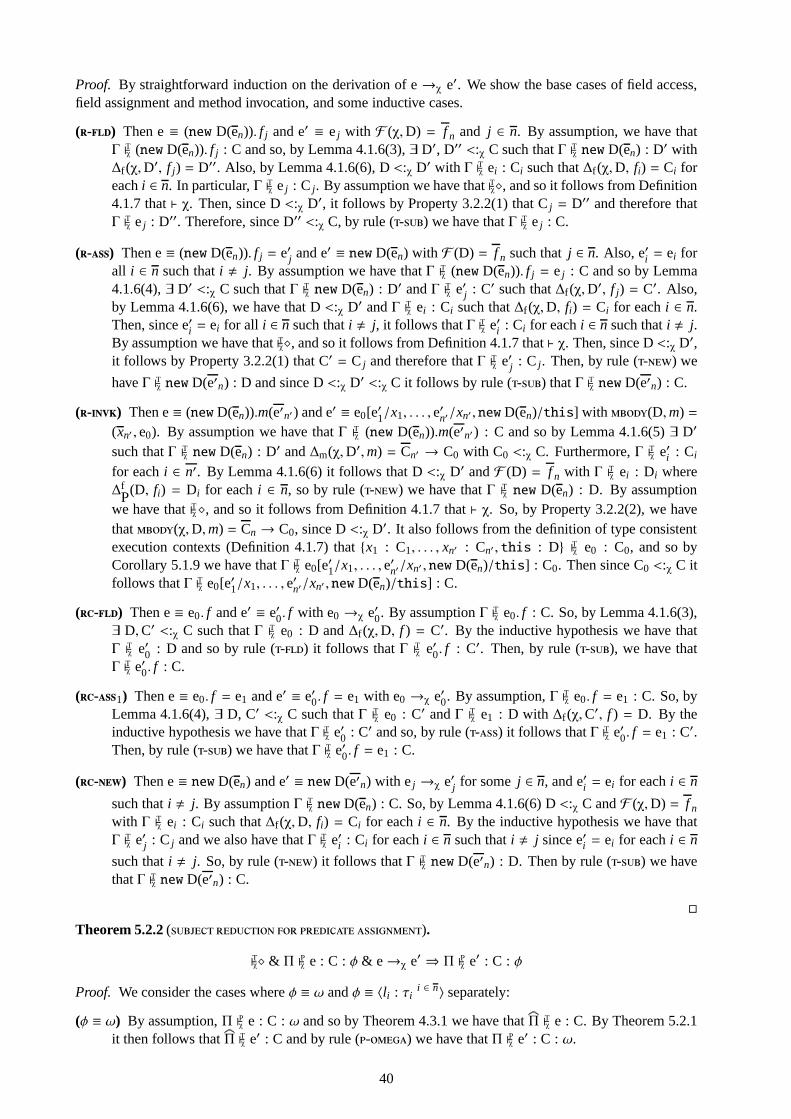
Proof. By straightforward induction on the derivation of e→χ e′. We show the base cases of field access,field assignment and method invocation, and some inductive cases.

(-) Then e≡ (new D(en)). f j and e′ ≡ ej with F (χ,D) = f n and j ∈ n. By assumption, we have thatΓ ⊢Tχ (new D(en)). f j : C and so, by Lemma 4.1.6(3),∃ D′, D′′ <:χ C such thatΓ ⊢Tχ new D(en) : D′ with∆f (χ,D′, f j) = D′′. Also, by Lemma 4.1.6(6), D<:χ D′ with Γ ⊢Tχ ei : Ci such that∆f (χ,D, fi) = Ci foreachi ∈ n. In particular,Γ ⊢Tχ ej : C j. By assumption we have that⊢Tχ⋄, and so it follows from Definition4.1.7 that⊢ χ. Then, since D<:χ D′, it follows by Property 3.2.2(1) that Cj = D′′ and therefore thatΓ ⊢Tχ ej : D′′. Therefore, since D′′ <:χ C, by rule (-) we have thatΓ ⊢Tχ ej : C.

(-) Then e≡ (new D(en)). f j = e′j and e′ ≡ new D(en) with F (D) = f n such thatj ∈ n. Also, e′i = ei forall i ∈ n such thati , j. By assumption we have thatΓ ⊢Tχ (new D(en)). f j = ej : C and so by Lemma4.1.6(4),∃ D′ <:χ C such thatΓ ⊢Tχ new D(en) : D′ andΓ ⊢Tχ e′j : C′ such that∆f (χ,D′, f j) = C′. Also,by Lemma 4.1.6(6), we have that D<:χ D′ andΓ ⊢Tχ ei : Ci such that∆f (χ,D, fi) = Ci for eachi ∈ n.Then, since e′i = ei for all i ∈ n such thati , j, it follows thatΓ ⊢Tχ e′i : Ci for eachi ∈ n such thati , j.By assumption we have that⊢Tχ⋄, and so it follows from Definition 4.1.7 that⊢ χ. Then, since D<:χ D′,it follows by Property 3.2.2(1) that C′ = C j and therefore thatΓ ⊢Tχ e′j : C j . Then, by rule (-) we

haveΓ ⊢Tχ new D(e′n) : D and since D<:χ D′ <:χ C it follows by rule (-) thatΓ ⊢Tχ new D(e′n) : C.

(-) Then e≡ (new D(en)).m(e′n′) and e′ ≡ e0[e′1/x1, . . . , e′n′/xn′ , new D(en)/this] with (D,m) =(xn′ , e0). By assumption we have thatΓ ⊢Tχ (new D(en)).m(e′n′) : C and so by Lemma 4.1.6(5)∃ D′

such thatΓ ⊢Tχ new D(en) : D′ and∆m(χ,D′,m) = Cn′ → C0 with C0 <:χ C. Furthermore,Γ ⊢Tχ e′i : Ci

for eachi ∈ n′. By Lemma 4.1.6(6) it follows that D<:χ D′ andF (D) = f n with Γ ⊢Tχ ei : Di where∆

fP(D, fi) = Di for eachi ∈ n, so by rule (-) we have thatΓ ⊢Tχ new D(en) : D. By assumption

we have that⊢Tχ⋄, and so it follows from Definition 4.1.7 that⊢ χ. So, by Property 3.2.2(2), we havethat(χ,D,m) = Cn → C0, since D<:χ D′. It also follows from the definition of type consistentexecution contexts (Definition 4.1.7) that{x1 : C1, . . . , xn′ : Cn′ , this : D} ⊢Tχ e0 : C0, and so byCorollary 5.1.9 we have thatΓ ⊢Tχ e0[e′1/x1, . . . , e′n′/xn′ , new D(en)/this] : C0. Then since C0 <:χ C itfollows thatΓ ⊢Tχ e0[e′1/x1, . . . , e′n′/xn′ , new D(en)/this] : C.

(-) Then e≡ e0. f and e′ ≡ e′0. f with e0 →χ e′0. By assumptionΓ ⊢Tχ e0. f : C. So, by Lemma 4.1.6(3),∃ D,C′ <:χ C such thatΓ ⊢Tχ e0 : D and∆f (χ,D, f ) = C′. By the inductive hypothesis we have thatΓ ⊢Tχ e′0 : D and so by rule (-) it follows thatΓ ⊢Tχ e′0. f : C′. Then, by rule (-), we have thatΓ ⊢Tχ e′0. f : C.

(-1) Then e≡ e0. f = e1 and e′ ≡ e′0. f = e1 with e0 →χ e′0. By assumption,Γ ⊢Tχ e0. f = e1 : C. So, byLemma 4.1.6(4),∃ D, C′ <:χ C such thatΓ ⊢Tχ e0 : C′ andΓ ⊢Tχ e1 : D with ∆f (χ,C′, f ) = D. By theinductive hypothesis we have thatΓ ⊢Tχ e′0 : C′ and so, by rule (-) it follows thatΓ ⊢Tχ e′0. f = e1 : C′.Then, by rule (-) we have thatΓ ⊢Tχ e′0. f = e1 : C.

(-) Then e≡ new D(en) and e′ ≡ new D(e′n) with ej →χ e′j for some j ∈ n, and e′i = ei for eachi ∈ n

such thati , j. By assumptionΓ ⊢Tχ new D(en) : C. So, by Lemma 4.1.6(6) D<:χ C andF (χ,D) = f nwith Γ ⊢Tχ ei : Ci such that∆f (χ,D, fi) = Ci for eachi ∈ n. By the inductive hypothesis we have thatΓ ⊢Tχ e′j : C j and we also have thatΓ ⊢Tχ e′i : Ci for eachi ∈ n such thati , j since e′i = ei for eachi ∈ n

such thati , j. So, by rule (-) it follows thatΓ ⊢Tχ new D(e′n) : D. Then by rule (-) we havethatΓ ⊢Tχ new D(e′n) : C.

�

Theorem 5.2.2( ).

⊢Tχ⋄ & Π ⊢Pχ e : C :φ & e→χ e′ ⇒ Π ⊢Pχ e′ : C : φ

Proof. We consider the cases whereφ ≡ ω andφ ≡ 〈l i : τii ∈ n〉 separately:

(φ ≡ ω) By assumption,Π ⊢Pχ e : C :ω and so by Theorem 4.3.1 we have thatΠ ⊢Tχ e : C. By Theorem 5.2.1it then follows thatΠ ⊢Tχ e′ : C and by rule (-) we have thatΠ ⊢Pχ e′ : C : ω.

40

(φ = σ ≡ 〈l i : τii ∈ n〉) This case proceeds by induction on the derivation of e→χ e′. Again, we show the

base cases of field access, field assignment and method invocation, and some inductive cases.

(-) Then e≡ (new D(en1)). f j and e′ ≡ ej with F (D) = f n1and j ∈ n1. By assumption,Π ⊢Pχ

(new D(en1)). f j : C : φ. So, by Lemma 4.2.10(3),∃ D′, C′ <:χ C,ψ P φ such that∆f (χ,D′, f j) =C′ andΠ ⊢Pχ newD(en1) : D′ : 〈 f j : ψ〉. Then, by Lemma 4.2.10(7), D<:χ D′ andΠ ⊢Pχ newD(en1) :D : 〈 f j : ψ〉, and by rule (-F) it follows thatΠ ⊢Pχ ej : C′′ : ψ with ∆f (χ,D, f j) = C′′ forsome C′′. By assumption we have that⊢Tχ ⋄, and so it follows from Definition 4.1.7 that⊢ χ.Then, since D<:χ D′, it follows from Property 3.2.2(1) that C′ = C′′ and so we have thatΠ ⊢Pχ ej : C′ : ψ. Then, since C′ <:χ C, we have by rule (-T) thatΠ ⊢Pχ ej : C : ψ.Furthermore, sinceψ P φ it follows by Theorem 4.3.2 thatΠ ⊢Pχ ej : C : φ.

(-) Then e≡ (new D(en1)). f j = e′j and e′ ≡ newD(e′n1) with F (χ,D) = f n1such thatj ∈ n1. Also

e′k = ek for eachk ∈ n1 such thatk , j.If σ = 〈ǫ〉, then by rule (-2) we have thatΠ ⊢Pχ new D(en1) : C : 〈ǫ〉. So, by Lemma 4.2.10(6)we have that D<:χ C andΠ ⊢Tχ new D(en1) : D. So, by rule (-) it follows thatΠ ⊢Tχ ek : Ck

such that∆f (χ,D, f ) = Ck for eachk ∈ n1. By Theorem 5.2.1 it follows thatΠ ⊢Tχ e′j : C j,since ej →χ e′j . Also, we have that e′k = ek for eachk ∈ n1 such thatk , j, and so it fol-lows thatΠ ⊢Tχ e′k : Ck for eachk ∈ n1 such thatk , j. Now, by rule (-), it follows thatΠ ⊢Tχ new D(e′n1) : D and so by rule (-O) we have thatΠ ⊢Pχ new D(e′n1) : D : 〈ǫ〉. Then,since D <:χ C it follows by rule (-T) thatΠ ⊢Pχ new D(e′n1) : C : 〈ǫ〉.If σ = 〈l i : τi

i ∈ n〉 , 〈ǫ〉, then by Lemma 4.2.10(4),∃ Dn such that Di <:χ C andΠ ⊢Pχ(new D(en1)). f j = e′j : Di : 〈l i : τi〉 for eachi ∈ n. Now, take anyi ∈ n; there are threepossibilities:

(l i = f ∈ ��-��, f = f j) Thenτi ≡ φ′, and by rule (-1), Π ⊢Pχ new D(en1) : Di : σ′ for

someσ′ andΠ ⊢Pχ e′j : D′ : φ′ with ∆f (χ,Di , f j) = D′. By Theorem 4.3.3 it follows thatΠ ⊢Tχ new D(en1) : Di and so by Lemma 4.1.6(6) we have that D<:χ Di andΠ ⊢Tχ ek : Ck with∆f (χ,D, fk) = Ck for eachk ∈ n1. Since e′k = ek for eachk ∈ n1 such thatk , j, it followsthatΠ ⊢Tχ e′k : Ck for eachk ∈ n1 such thatk , j. By assumption we have that⊢Tχ ⋄, andso it follows from Definition 4.1.7 that⊢ χ. Then, since D<:χ Di it follows from Property3.2.2(1) that D′ = C j and therefore thatΠ ⊢Pχ e′j : C j : φ′. So, by rule (-F) we have

thatΠ ⊢Pχ new D(e′n1) : D : 〈 f j : φ′〉. Then, since D<:χ Di it follows by rule (-T) thatΠ ⊢Pχ new D(e′n1) : Di : 〈 f j : φ′〉.

(l i = f ∈ ��-��, f , f j) Thenτi = φ′ and l i = f j′ for some j′ ∈ n1 such that j′ , j.By rule (-2) we have thatΠ ⊢Pχ new D(en1) : Di : 〈 f j′ : φ′〉 andΠ ⊢Tχ e′j : D′ with∆f (χ,Di , f j) = D′. By Lemma 4.2.10(7) D<:χ Di andΠ ⊢Pχ new D(en1) : D : 〈 f j′ : φ′〉.By rule (-F) we then have thatΠ ⊢Pχ ej′ : C j′ : φ′ with ∆f (χ,D, f j′) = C j′ , andΠ ⊢Tχ ek : Ck with ∆f (χ,D, fk) = Ck for all k ∈ n1 such thatk , j′. Since e′k = ek for eachk ∈ n1 such thatk , j, it follows thatΠ ⊢Pχ e′j′ : C j′ : φ′ and also thatΠ ⊢Tχ e′k : Ck foreachk ∈ n1 such thatk , j′ andk , j. By assumption we have that⊢Tχ⋄, and so it followsfrom Definition 4.1.7 that⊢ χ. Then, since D<:χ Di, it follows from property 3.2.2(1)that D′ = C j and so we have thatΠ ⊢Tχ e′j : C j. Then, by rule (-F) we have that

Π ⊢Pχ new D(e′n1) : D : 〈 f j′ : φ′〉. Furthermore, since D<:χ Di it follows by rule (-T)thatΠ ⊢Pχ new D(e′n1) : Di : 〈 f j′ : φ′〉.

(l i ∈��-��) Thenl i = mandτi ≡ ψ::φn2→ φ′. By rule (-2),Π ⊢Pχ newD(en1) :

Di : 〈m : τiψ::φn2→ φ′〉 andΠ ⊢Tχ e′j : D′ with ∆f (χ,Di , f j) = D′. By Lemma 4.2.10(7)

D <:χ Di andΠ ⊢Pχ new D(en1) : D : 〈m : ψ::φn2→ φ′〉. By rule (-M) we

have thatΠ′ ⊢Pχ e0 : D0 : φ′ with ∆m(χ,D,m) = Cn2 → D0 andΠ′ = { x1 : C1 :φ1, . . . , xn2 : Cn2 : φn2, this : D : ψ } such that(χ,D,m) = (xn2, e0). We alsohave thatΠ ⊢Tχ new D(en1) : D. Then, by rule (-) it follows thatΠ ⊢Tχ ek : C′k with∆f (χ,D, fk) = C′k for eachk ∈ n1. Since e′k = ek for eachk ∈ n1 such thatk , j, it followsthatΠ ⊢Tχ e′k : Ck for eachk ∈ n1 such thatk , j. By assumption we have that⊢Tχ⋄, and so it fol-lows from Definition 4.1.7 that⊢ χ. Then, since D<:χ Di it follows from Property 3.2.2(1)

41

that D′ = C′j and soΠ ⊢Tχ e′j : C′j. So, by rule (-) we have thatΠ ⊢Tχ new D(e′n1) : D and

by rule (-M) it follows thatΠ ⊢Pχ new D(e′n1) : D : 〈m : ψ::φn2→ φ′〉. Furthermore,

since D<:χ Di it follows by rule (-T) thatΠ ⊢Pχ new D(e′n1) : Di : 〈m : ψ::φn2→ φ′〉.

Since our choice ofi was arbitrary, we have thatΠ ⊢Pχ new D(e′n1) : Di : 〈l i : τi〉 for all i ∈ n.Then, since each Di <:χ C we have by rule (-T) thatΠ ⊢Pχ new D(e′n1) : C : 〈l i : τi〉 foreachi ∈ n and by rule (-) it then follows thatΠ ⊢Pχ new D(e′n1) : C : 〈l i : τi

i ∈ n〉.

(-) Then e≡ (new D(en1)).m(e′n2) and also e′ ≡ e0[e′1/x1, . . . , e′n2/xn2, new D(en1)/this] with

(D,m) = (xn2, e0). By assumption we haveΠ ⊢Pχ (new D(en1)).m(e′n2) : C : φ and soby Lemma 4.2.10(5)∃ D′, Cn2, C′′ <:χ C, ψ, φn2

andφ′ P φ such thatΠ ⊢Pχ new D(en1) :D′ : 〈m : ψ::φn2

→ φ′〉 andΠ ⊢Pχ new D(en1) : D′ : ψ with ∆m(χ,D′,m) = Cn2 → C′′.Furthermore, we have thatΠ ⊢Pχ ek : Ck : φk for eachk ∈ n2. By Theorem 4.3.1 it follows thatΠ ⊢Tχ new D(en1) : D′. Then, by Lemma 4.1.6(6) we have that D<:χ D′ andF (χ,D) = f n1

with Π ⊢Tχ ek : Dk such that∆f (χ,D, fk) = Dk for eachk ∈ n1. Therefore, by rule (-) itfollows thatΠ ⊢Tχ new D(en1) : D and so by Theorem 4.3.3 we have thatΠ ⊢Pχ new D(en1) : D : ψandΠ ⊢Pχ new D(en1) : D : 〈m : ψ::φn2

→ φ′〉. Then, by rule (-M) it follows thatΠ′ ⊢Pχ e0 : C′ : φ′ with Π′ = {x1 : C′1 : φ1, . . . , xn2 : C′n2

: φn2, this : D : ψ} such that

∆m(χ,D,m) = C′n2 → C′. Since, by assumption we have⊢Tχ ⋄, it follows from Definition 4.1.7that⊢ χ and so from Property 3.2.2(2) that C′′ = C′ and Ck = C′k for eachk ∈ n2, since D<:χ D′.Thus,Π′ = {x1 : C1 : φ1, . . . , xn2 : Cn2 : φn2, this : D : ψ}, and by Corollary 5.1.9(2) it followsthatΠ ⊢Pχ e0[e1/x1, . . . , en2/xn2, new D(en1)/this] : C′ : φ′. Then, since C′ = C′′ <:χ C we haveby rule (-T) thatΠ ⊢Pχ e0[e1/x1, . . . , en2/xn2, new D(en1)/this] : C : φ′. Furthermore,sinceφ′ P φ it follows from Theorem 4.3.2 thatΠ ⊢Pχ e0[e1/x1, . . . , en2/xn2, new D(en1)/this] :C : φ.

(-2) Then e≡ e0. f = e1 and e′ ≡ e0. f = e′1 with e1 →χ e′1. By assumption,Π ⊢Pχ e0. f = e1 : C :

σ. By Lemma 4.2.10(4),∃ Cn such that Ci <:χ C andΠ ⊢Pχ e0. f = e1 : Ci : 〈l i : τi〉 for eachi ∈ n.Now, take anyi ∈ n; there are two possibilities:

( f = l i) Thenτ = φ′. By rule (-1), Π ⊢Tχ e0 : Ci andΠ ⊢Pχ e1 : D : φ′ with ∆f (χ,Ci , f ) = D.By the inductive hypothesis we have thatΠ ⊢Pχ e′1 : D : φ′ and so by rule (-1) it followsthatΠ ⊢Pχ e0. f = e′1 : Ci : 〈 f : φ′〉. Then, since Ci <:χ C, by rule (-T) we have thatΠ ⊢Pχ e0. f = e′1 : C : 〈 f : φ′〉.

( f , l i) By rule (-2),Π ⊢Pχ e0 : Ci : 〈l i : τi〉 andΠ ⊢Tχ e1 : D with∆f (χ,Ci , f ) = D. By Theorem5.2.1 we have thatΠ ⊢Tχ e′1 : D and so by rule (-2) it follows thatΠ ⊢Pχ e0. f = e′1 : Ci : 〈l i :τi〉. Then, since Ci <:χ C, we have by rule (-T) thatΠ ⊢Pχ e0. f = e′1 : C : 〈l i : τi〉.

Since our choice ofi was arbitrary, we have thatΠ ⊢Pχ e0. f = e′1 : C : 〈l i : τi〉 for all i ∈ n, and byrule (-) thatΠ ⊢Pχ e0. f = e′1 : C : 〈l i : τi

i ∈ n〉.

(-2) Then e≡ e0.m(en1) and e′ ≡ e0.m(e′n1) with ej →χ e′j for some j ∈ n1, and e′i = ei foreachi ∈ n1 such thati , j. By assumptionΠ ⊢Pχ e0.m(en1) : C : φ. So, by Lemma 4.2.10(5),∃ D,Cn1, C′ <:χ C,ψ, φn1

, φ′ P φ such thatΠ ⊢Pχ e′0 : D : 〈m : ψ::φn1→ φ′〉 andΠ ⊢Pχ e′0 : D : ψ with

Π ⊢Pχ ei : Ck : φk for eachk ∈ n1 such that∆m(χ,D,m) = Cn1 → C′. By the inductive hypothesiswe then have thatΠ ⊢Pχ e′j : C j : φ j, and we also have thatΠ ⊢Pχ e′i : Ci : φi for eachi ∈ n1 such that

i , j since, in each case, e′i = ei . Thus, by rule (-), it follows thatΠ ⊢Pχ e0.m(e′n1) : C′ : φ′.Then, since C′ <:χ C we have by rule (-T) thatΠ ⊢Pχ e0.m(e′n1) : C : ψ. Furthermore,sinceφ′ P φ, by Theorem 4.3.2 it follows thatΠ ⊢Pχ e0.m(e′n1) : C : φ.

�

5.3 Subject Expansion

As is the case for theς-calculus [1], subject expansion does not hold in general for type assignment. Wecan, however, show that subject expansion for predicate assignment holds under the assumption that both the

42

redex and the reduct have the same type. This extra assumption is necessary, since predicates are assignedto typeableterms (see Theorem 4.3.1). This is also a requirement of the subject expansion result for thepredicate system in [5]

Theorem 5.3.1( ).

⊢Tχ⋄ & Π ⊢Pχ e′ : C : φ & e→χ e′ & Π ⊢Tχ e : C⇒ Π ⊢Pχ e : C :φ

Proof. We consider the cases whereφ ≡ ω andφ ≡ 〈l i : τii ∈ n〉 separately:

(φ ≡ ω) This case is trivial, since by assumption we have thatΠ ⊢Tχ e : C and so, by rule (-), it followsthatΠ ⊢Pχ e : C :ω.

(φ ≡ 〈l i : τii ∈ n〉) This case proceeds by induction on the derivation of e→χ e′. As for the proofs of subject

reduction, we show the base cases of (-), (-) and (-), and some inductive cases.

(-) Then e≡ (new D(en1)). f j and e′ ≡ ej with F (χ,D) = f n1and j ∈ n1. By assumption,

Π ⊢Tχ (new D(en1)). f j : C. So, by Lemma 4.1.6(3),∃ D′,C′ <:χ C such thatΠ ⊢Tχ new D(en1) : D′

and∆f (χ,D′, f ) = C′. Then, by Lemma 4.1.6(6) it follows that D<:χ D′ andΠ ⊢Tχ ek : Ck

with ∆f (χ,D, fk) = Ck for eachk ∈ n1. Also by assumption we have thatΠ ⊢Pχ ej : C : φ,so by Theorem 4.3.3 it follows thatΠ ⊢Pχ ej : C j : φ. Then by rule (-F) we have thatΠ ⊢Pχ new D(en1) : D : 〈 f j : φ〉, and by rule (-) thatΠ ⊢Pχ (new D(en1)). f j : C j : φ. Byassumption we have that⊢Tχ ⋄, and so it follows from Definition 4.1.7 that⊢ χ. Then, since∆f (χ,D′, f j) = C′ and∆f (χ,D, f j) = C j with D <:χ D′, it follows from Property 3.2.2(1) thatC j = C′, and soΠ ⊢Pχ (new D(en1)). f j : C′ : φ. Then, since C′ <:χ C, by rule (-T) we havethatΠ ⊢Pχ (new D(en1)). f j : C : φ.

(-) Then e≡ (new D(en1)). f j = e′j and e′ ≡ newD(e′n1) with F (χ,D) = f n1such thatj ∈ n1. Also

e′k = ek for eachk ∈ n1 such thatk , j.If σ = 〈ǫ〉, then we need to show thatΠ ⊢Pχ (new D(en1)). f j = e′j : C : 〈ǫ〉. By assumption wehave thatΠ ⊢Tχ (new D(en1)). f j = e′j : C, and so by Lemma 4.1.6(4) we have that∃ D′ <:χ C suchthatΠ ⊢Tχ new D(en1) : D′ andΠ ⊢Tχ e′j : C′j with ∆f (χ,D′, f j) = C′j. By Lemma 4.1.6(6) is alsofollows that D<: D′ andΠ ⊢Tχ ek : Ck with ∆f (χ,D, fk) = Ck for eachk ∈ n1. So, by rule (-)it follows thatΠ ⊢Tχ new D(en1) : D and so by rule (-O) thatΠ ⊢Pχ new D(en1) : D : 〈ǫ〉.By assumption we have that⊢Tχ ⋄, and so it follows from Definition 4.1.7 that⊢ χ. Then, sinceD <:χ D′, it follows from Property 3.2.2(1) that C′j = C j, and soΠ ⊢Tχ e′j : C j. So, we now haveby rule (-2) thatΠ ⊢Pχ (new D(en1)). f j = e′j : D : 〈ǫ〉. Lastly, since D<:χ D′ <:χ C, it followsby rule (-T) thatΠ ⊢Pχ (new D(en1)). f j = e′j : C : 〈ǫ〉.

If σ = 〈l i : τii ∈ n〉 , 〈ǫ〉, then by Lemma 4.2.10(7) it follows that D<:χ C andΠ ⊢Pχ new D(e′n1) :

D : 〈l i : τi〉 for eachi ∈ n1. Now, take anyi ∈ n1; there are three possibilities:

(l i = f ∈ ��-��, f = f j) Then τi = φ′, and by rule (-F), Π ⊢Pχ e′j : C j : φ′ andΠ ⊢Tχ e′k : Ck with ∆f (χ,D, fk) = Ck for eachk ∈ n1 such thatk , j′. By assumption,Π ⊢Tχ(new D(en1)). f j = e′j : C. So by Lemma 4.1.6(4),∃ D′ <:χ C such thatΠ ⊢Tχ new D(en1) : D′

andΠ ⊢Tχ e′j : C′ with ∆f (χ,D′, f j) = C′. By assumption we have that⊢Tχ⋄, and so it followsfrom Definition 4.1.7 that⊢ χ. Then, since by Lemma 4.1.6(6) we have that D<:χ D′, itfollows by Property 3.2.2(1) that C′ = C j, and so also thatΠ ⊢Pχ e′j : C′ : φ′. Therefore, byrule (-1) we have thatΠ ⊢Pχ (new D(en1)). f j = e′j : D′ : 〈 f j : φ′〉 and since D′ <:χ C itfollows by rule (-T) thatΠ ⊢Pχ (new D(en1)). f j = e′j : C : 〈 f j : φ′〉.

(l i = f ∈ ��-��, f , f j) Thenτi = φ′, and by rule (-F) we have thatf = f j′ with

j ∈ n1 such thatj′ , j. So,Π ⊢Pχ e′j′ : C j′ : φ′ with ∆f (χ,D, f j′) = C j′ andΠ ⊢Tχ e′k : Ck with∆f (χ,D, fk) = Ck for eachk ∈ n1 such thatk , j′. By assumption,Π ⊢Tχ (new D(en1)). f j =

e′j : C. So by Lemma 4.1.6(4),∃ D′ <:χ C such thatΠ ⊢Tχ new D(en1) : D′ andΠ ⊢Tχ e′j : C′

with ∆f (χ,D′, f j) = C′. Then, by Lemma 4.1.6(6), D<:χ D′ andΠ ⊢Tχ ek : Ck such that∆f (χ,D, fk) = Ck for eachk ∈ n1. Now, since ej′ = e′j′ , it follows immediately thatΠ ⊢Pχej′ : C j′ : φ′. So, by rule (-F) we have thatΠ ⊢Pχ new D(en1) : D : 〈 f j′ : φ′〉. Byassumption we have that⊢Tχ⋄, and so it follows from Definition 4.1.7 that⊢ χ. Then, since

43

D <:χ D′, it follows from Property 3.2.2(1) that C′ = C j, and soΠ ⊢Tχ e′j : C j. Then by rule(-2) we have thatΠ ⊢Pχ (new D(en1)). f j = e′j : D : 〈 f j′ : φ′〉. Furthermore, since D<:χ Cit follows by rule (-T) thatΠ ⊢Pχ (new D(en1)). f j = e′j : C : 〈 f j′ : φ′〉.

(l i = m ∈��-��) Thenτi = 〈m : ψ::φn2→ φ′〉, and by rule (-M) we

have thatΠ ⊢Tχ new D(e′n1) : D andΠ′ ⊢Pχ e0 : C′ : φ′ such that∆m(χ,D,m) = Cn2 → C′ and(χ,D,m) = (xn2, e0) whereΠ′ = {x1 : C1 : φ1, . . . , xn2 : Cn2 : φn2, this : D : ψ}.By assumption,Π ⊢Tχ (new D(en1)). f j = e′j : C. So by Lemma 4.1.6(4),∃ D′ <:χ C suchthatΠ ⊢Tχ new D(en1) : D′ andΠ ⊢Tχ e′j : C′ with ∆f (χ,D′, f j) = C′. Then, by Lemma4.1.6(6), D<:χ D′ andΠ ⊢Tχ ek : Ck such that∆f (χ,D, fk) = Ck for eachk ∈ n1, and byrule (-) it follows thatΠ ⊢Tχ new D(en1) : D. By rule (-M) it now follows thatΠ ⊢Pχ new D(en1) : D : 〈m : ψ::φn2

→ φ′〉, and since D<:χ D′ we have by rule (-T)thatΠ ⊢Pχ new D(en1) : D′ : 〈m : ψ::φn2

→ φ′〉. Now, by rule (-2) it follows thatΠ ⊢Pχ (new D(en1)). f j = e′j : D′ : 〈m : ψ::φn2

→ φ′〉. Furthermore, since D′ <:χ C we have by

rule (-T) thatΠ ⊢Pχ (new D(en1)). f j = e′j : C : 〈m : ψ::φn2→ φ′〉.

Since the choice ofi was arbitrary, we have thatΠ ⊢Pχ (new D(en1)). f j = e′j : C : 〈l i : τi〉 for each

i ∈ n. Then by rule (-) it follows thatΠ ⊢Pχ (new D(en1)). f j = e′j : C : 〈l i : τii ∈ n〉.

(-) Then e≡ (new D(en1)).m(e′n2) and e′ ≡ e0[e′1/x1, . . . , e′n2/xn2, new D(en1)/this] with

(D, m) = (xn2, e0). By assumption, we have thatΠ ⊢Pχ e0[e′1/x1, . . . , e′n2/xn2, new D(en1)/this] :

C : φ. Also, by assumption, we have thatΠ ⊢Tχ (new D(en1)).m(e′n2) : C. So, by Lemma 4.1.6(5),∃ D′, Cn2, and C′′ <:χ C such thatΠ ⊢Tχ new D(en1) : D′ and∆m(χ,D′,m) = Cn2 → C′′ withΠ ⊢Tχ ek : Ck for eachk ∈ n2. Also, by Lemma 4.1.6(6), it follows that D<:χ D′ andF (χ,D) = f n1

with Π ⊢Tχ ek : Dk such that∆f (χ,D, fk) = Dk for eachk ∈ n1. Therefore, by rule (-) we havethatΠ ⊢Tχ new D(en1) : D. Since, by assumption, we have⊢Tχ ⋄ it follows from Definition 4.1.7thatΓ′ ⊢Tχ e0 : C′ where∆m(χ,D,m) = C′n2 → C′ andΓ′ = {x1 : C′1, . . . , xn2 : C′n2

, this : D}.We also have from Definition 4.1.7 that⊢ χ and so from Property 3.2.2(2) that C′′ = C′, andCk = C′k for eachk ∈ n2, since D <:χ D′. Then it follows thatΠ ⊢Tχ e′k : C′k for eachk ∈ n2.It also follows, then, that C′ <:χ C and so by rule (-) we have thatΓ′ ⊢Tχ e0 : C. Now, itfollows from Corollary 5.1.12 that∃ φn2

andψ such thatΠ′ ⊢Pχ e0 : C : φ whereΠ′ = {x1 : C′1 :φ1, . . . , xn2 : C′n2

: φn2, this : D : ψ}, with Π ⊢Pχ (new D(en1)) : D : ψ andΠ ⊢Pχ ek : C′k : φk foreachk ∈ n2. So, by rule (-M) we have thatΠ ⊢Pχ (new D(en1)) : D : 〈m : ψ::φn2

→ φ〉,and by rule (-), thatΠ ⊢Pχ (new D(en1)).m(e′n2) : C′ : φ. Then, since C′ <: C we have by rule(-T) thatΠ ⊢Pχ (new D(en1)).m(e′n2) : C : φ.

(-) Then e≡ e0. f and e′ ≡ e′0. f with e0 →χ e′0. By assumption we have thatΠ ⊢Pχ e′0 : C : φand so by Lemma 4.2.10(3),∃ D,C′ <:χ C andψ P φ such that∆f (χ,D, f ) = C′ andΠ ⊢Pχ e′0 :D : 〈 f : ψ〉. Also, by assumption we have thatΠ ⊢Tχ e0. f : C and so by Lemma 4.1.6(3),∃D′,C′′ <:χ C such thatΠ ⊢Tχ e0 : D′ and∆f (χ,D′, f ) = C′′. Since e0 →χ e0, by Theorem 5.2.1 itfollows thatΠ ⊢Tχ e′0 : D′. Then, by Theorem 4.3.3 we have thatΠ ⊢Pχ e′0 : D′ : 〈 f : ψ〉. Now, bythe inductive hypothesis it follows thatΠ ⊢Pχ e0 : D′ : 〈 f : ψ〉 and so by rule (-) we have thatΠ ⊢Pχ e0. f : C′′ : ψ. Then, since C′′ <:χ C it follows by rule (-T) thatΠ ⊢Pχ e0. f : C : ψ.Furthermore, sinceψ P φ we have by Theorem 4.3.2 thatΠ ⊢Pχ e0. f : C : φ.

(-2) Then e≡ e0.m(en1) and e′ ≡ e0.m(e′n1) with ej →χ e′j for somej ∈ n1 and e′k = ek for each

k ∈ n1 such thatk , j. By assumption we have thatΠ ⊢Pχ e′0.m(e′n1) : C : φ and so by Lemma

4.2.10(5),∃ D, Cn1,C′ <:χ C, ψ, φn1

, φ′ P φ such thatΠ ⊢Pχ e0 : D : 〈m : ψ::φn1→ φ′〉 and

Π ⊢Pχ e0 : D : ψ with Π ⊢Pχ e′k : Ck : φk for eachk ∈ n1 such that∆m(χ,D,m) = Cn1 → C′. Also

by assumption we have thatΠ ⊢Tχ e0.m(en1) : C and so by Lemma 4.1.6(5),∃ D′, C′n1, C′′ <:χ Csuch thatΠ ⊢Tχ e0 : D′ andΠ ⊢Tχ ek : C′k for eachk ∈ n1 such that∆m(χ,D′,m) = C′n1 → C′′. SinceΠ ⊢Tχ ej : C′j and ej →χ e′j it follows by Theorem 5.2.1 thatΠ ⊢Tχ e′j : C′j , and so by Theorem 4.3.3we have thatΠ ⊢Pχ e′j : C′j : φ j . Then by the inductive hypothesis it follows thatΠ ⊢Pχ ej : C′j : φ j.Also, since ek = e′k for eachk ∈ n1 such thatk , j, it follows thatΠ ⊢Pχ ek : Ck : φk for eachk ∈ n1

such thatk , j, and then by Theorem 4.3.3, thatΠ ⊢Pχ ek : C′k : φk for eachk ∈ n1 such thatk , j.

44

Lastly, sinceΠ ⊢Pχ e0 : D : 〈m : ψ::φn1→ φ′〉 andΠ ⊢Tχ e0 : D′ it also follows by Theorem 4.3.3 that

Π ⊢Pχ e0 : D′ : 〈m : ψ::φn1→ φ′〉. So, by rule (-), we then have thatΠ ⊢Pχ e0.m(en1) : C′′ : φ′

and since C′′ <:χ C it follows by rule (-T) thatΠ ⊢Pχ e0.m(en1) : C : φ′. Furthermore,sinceφ′ P φ we have by Theorem 4.3.2 thatΠ ⊢Pχ e0.m(en1) : C : φ

�

5.4 Characterisation of Expressions

As with the intersection type system for theλ-calculus, the subject expansion result for the predicate systemallows us to characterise the behaviour of LJ expressions bythe predicates that we can assign to them. Wecan investigate this property of the predicate system by comparing similar results from theλ-calculus. It isimportant to note that we have not proved these characterisation results for the LJ predicate system, howeverwe believe that they will hold due to the similarity between this system and the intersection type systems fortheλ-calculus.

We first see that (using an object predicate environment) anyLJ expression that terminates in an objectcan be assigned a non-trivial predicate thatdoes notincludeω. To see this, we first notice that such anexpression has a reduction sequence of the form e→∗χ o ≡ e →χ en →χ . . . →χ e1 →χ o for some(possibly empty) sequence of expressionsen. It is easy to see that the object o can be assigned such anon-trivial predicate (using an object predicate environment). Then, using the subject expansion theorem,we can see that the same predicate is assignable to each of theexpressions ei in turn, and so then also to e.Such expressions correspond toλ-terms which have a normal form (a term on which no further reductionis possible). Any term in normal form may be assigned an intersection type without usingω, and by theexpansion result for the intersection type assignment system, so can any term which reduces to it.

We now turn our attention to expressions which are non-terminating. These correspond toλ terms whichdo not have a normal form. An example of such a term is (λx.xx)(λx.xx), whichβ-reduces to itself in a singlestep, and thus has neither a normal form, nor a head-normal form. Consider the following program:

χ = class C extends Object

{

C m() { this.m() }}

e = (new C()).m()

The expression e also runs to itself, thus e→χ e→χ . . . ad infinitum. Notice that∅ ⊢Tχ e : C, and so by rule(-) we have∅ ⊢Pχ e : C : ω. However,ω is theonly predicate that we can assign to e. This is also thecase forλ-terms without a normal form or a head-normal form.

Finally we look at LJ expressions that correspond to those terms in theλ-calculus that have a head-normal form. These terms correspond to computations that are non-terminating, yet still return some formof meaningful result. An example of such aλ-term is the fixed point operatorλ f .(λx. f (xx))(λx. f (xx)). Thisterm has the following sequence of reductions:

λ f .(λx. f (xx))(λx. f (xx))→β λ f . f (λ f .(λx. f (xx))(λx. f (xx)))→β λ f . f ( f (λ f .(λx. f (xx))(λx. f (xx))))→β λ f . f ( f ( f (λ f .(λx. f (xx))(λx. f (xx)))))→β . . .

Now, consider the following LJ program:

45

χ = class C extends Object

{

C f

C m() { this.f = this.m() }}

e = (new C()).m()

which results in this sequence of reductions:

e ≡ (new C((C) null)).m()→χ (new C((C) null)).f = (new C((C) null)).m()→χ e1 ≡ new C((new C((C) null)).m())→χ new C((new C((C) null)).f = (new C((C) null)).m())→χ e2 ≡ new C(new C((new C((C) null)).m()))→∗χ e3 ≡ new C(new C(new C((new C((C) null)).m())))

..

.

Thus, this expression constructs an ever increasingly nested object. Observe that∅ ⊢Tχ e : C and so by rule(-) it follows that∅ ⊢Pχ e : C : ω. Given this, we can assign the following predicates to the sequence ofexpressionsen:

∅ ⊢Pχ e1 : C : 〈f : ω〉

∅ ⊢Pχ e2 : C : 〈f : 〈f : ω〉〉

∅ ⊢Pχ e3 : C : 〈f : 〈f : 〈f : ω〉〉〉

..

.

Then, by subject expansion, we can assign all of these predicates to the expression e itself. Thus, we canassign a non-trivial predicate to e, but it must containω, indicating that there is non-termination somewhere.Again, this is the case for the intersection type assignmentsystem for theλ-calculus.

A final point that we can make concerns the expressiveness of the predicate system over the type system.A result of the type system (and similarly of the type systemsof FJ, MJ and Java itself) is that if an expressionis typeable, then executing the expression will not result in any illegal field accesses or method invocations.In other words, whenever a field is accessed, or a method invoked, such a field or method will always existin the receiving object. One thing thatmayhappen, however, is a null reference exception. This occurswhena field is accessed or a method invoked on a null object. The type system does not distinguish between thetypes of null objects and the types of non-null objects; thusit cannot determine when such a mismatch willoccur. The predicate system, on the other hand,doesmake such a distinction: the only non-trivial predicatethat null objects may be assigned is the empty predicate〈ǫ〉. As such, a field access or a method invocationon a null object cannot be assigned any predicate other thanω, since the premise for such a predicateassignment is that the receiver have an appropriate non-empty object predicate. Thus, again by subjectexpansion, it follows that the execution of any expression which can be assigned a non-trivial predicate willnot result in a null reference exception.

46

Chapter 6

Decidable Restrictions of the PredicateSystem

In Chapter 5 we showed a subject expansion result for the predicate assignment system. This suggeststhat predicate assignment is undecidable, as is the case forintersection type assignment systems for theλ-calculus and the predicate system for theς-calculus in [5] (which also display subject expansion properties).In this chapter, we define a two-tier restriction of the predicate system which we believeis decidable. That is,there exists an algorithm which will terminate resulting ina yes/no answer indicating whether a non-trivialpredicate can be assigned to that expression. We will present such an algorithm, which takes as input anexecution context, a (type) environment and an expression,and argue that it is terminating. If the algorithmterminates in the affirmative, then it also returns a predicate. We conjecture that the algorithm issoundinthat whenever it returns a predicate, there exists a predicate derivation which assigns that predicate to theinput expression.

6.1 Decidability of Type Assignment

Since expressions are annotated with type information, type assignment is decidable, and collapses to thesimple process of type checking. That is, in order to infer a type for an expression, we need only look at thetypes declared in the syntax when a new (possibly null) object is created, and then subsequently look up thetypes of its fields and methods (checking that objects assigned to fields or passed as arguments to methodshave an appropriate type).

What we notice, however, is that open terms do not necessarily have a unique type: the type of anexpression will depend upon the types of the variables. To see that this is the case, consider the followingexecution context:

χ = class A extends Object class C extends Object

{ {

B f D f

} }

class B extends Object { }

class D extends Object { }

Then, when we come to assign a type to the expressionx.f, the type that we can assign depends upon thetype ofx . So,bothof the following are valid statements:

{x : A} ⊢Tχ x.f : B

{x : C} ⊢Tχ x.f : D

Thus, an open expression does not, in general, have auniquetype. Finding each possible type environmentand assignable type for an expression is still a decidable problem, however such an algorithm would need toutilise back-tracking techniques and would necessarily bemore complex than one which is constrained to

47

find a single solution. Therefore, to simplify the type inference algorithm, we require that a type environmentis provided. This will also be the case for the predicate inference algorithms of§6.2 and§6.3.

We now present the type inference algorithm itself:

Definition 6.1.1 ( ). The class type inference algorithm,Type, takes an executioncontext and a type environment, and returns the type of the given expression. It is defined as follows:

Type χ Γ (C) null = C

Type χ Γ x = C if x : C ∈ Γ

Type χ Γ e. f = D if ∆f (χ,C, f ) = Dwhere C= Type(χ, Γ, e)

Type χ Γ e1. f = e2 = C if D <:χ ∆f (χ,C, f )where C= Type(χ, Γ, e1)

D = Type(χ, Γ, e2)

Type χ Γ e0.m(en) = D if C i <:χ C′i ∀ i ∈ nwhere C= Type(χ, Γ, e0)

Ci = Type(χ, Γ, ei) ∀ i ∈ n∆m(χ,C,m) = C′n→ D

Type χ Γ new C(en) = C if Ci <:χ C′i ∀ i ∈ nwhere F (χ,C) = f n

∆f (χ,C, fi) = C′i ∀ i ∈ nCi = Type(χ, Γ, ei) ∀ i ∈ n

The algorithm fails whenever any of the side-conditions arenot met, that is any of the following:

• Variable look-up in the type environment fails (i.e. no statement with the specified variable as thesubject exists in the type environment),

• Type lookup fails to return a type from the field table∆f or method table∆m (i.e. no such field ormethod exists in the given class),

• The number of arguments to a method call does not match the length of the sequence of argumenttypes returned by the method table∆m,

• The number of sub-expressions in the sequenceen of a new object creation expressionnewD(en) doesnot match the length of the sequence returned by the field listlook-up functionF ,

• A subtype check Ci <:χ C′i fails (i.e. Ci is not a subtype of C′i ).

This algorithm illustrates the rationale behind the choiceto define null object expressions with a typeannotation. Since the algorithm is defined inductively, without such type annotations we cannot know, at thepoint where we must assign a type to a null object expression,which object it must behave as (i.e. whichfields and methods will be called on it). Therefore, we would have to incorporate back-tracking techniquesinto the algorithm in order that we could reassign the correct type once we have examined the context inwhich the null object appears, and the correct type can be inferred.

It is not difficult to see that this algorithm terminates, and we now argue informally to this effect. Firstly,we note that the algorithm operates recursively, i.e. by calling itself. At each recursive call, however, thesize of the expression on which it operates becomes smaller.Therefore, the recursion is limited by thelength of the expression upon which the algorithm operates.It then remains for us to check that the otherelements of the algorithm are terminating, namely the type environment look-up, the checking whether onetype is a subtype of another, the looking up of types in the field and method tables, and the looking up offield lists. The type environment look-up procedure is clearly terminating if the type environment containsa finite number of statements. As we will explain in a moment, the termination of the other operations is

48

dependent upon the well formedness of the execution contextpassed to the algorithm, and one property ofwell formed contexts in particular: the acyclic nature of the class hierarchy. This property ensures that thereare no cycles in the inheritance hierarchy of each class defined in the execution context. Since the fieldlist look-up function, and the field and method tables are also defined recursively (see Definitions 3.1.4 and3.1.5 respectively), the acyclic nature of the class hierarchy means that there will be no infinite looping inthe implementation of these functions. Then, since there must be a finite number of classes in the executioncontext (and there are a finite number of fields and methods in each class), the level of recursion is limitedby the number of classes defined.

To check whether the class hierarchy is acyclic is also a decidable problem, since the maximum lengthof an acyclic inheritance hierarchy is bounded by the numberof classes defined in the context. To constructthe inheritance hierarchy for a class, we extract the name ofits superclass from the class definition, thenlook up the definition of the superclass and extract the name of its superclass, etc. We do this until we obtaina class name which is not defined in the context,or we have obtained a sequence whose length matches thenumber of classes defined in the context. Since we bound the length of the sequence in this way, we are surethat our look-up operation will terminate. Then, to check that the hierarchy is acyclic, we simply check thateach class name in the sequence isunique, which again is a terminating operation, bounded by the numberof class names in the sequence.

We assert that the type inference algorithm is bothsoundandcompletewith respect to type assignment:

Property 6.1.2( ). χ ⊢ Γ & Type(χ, Γ, e)= C⇒ Γ ⊢Tχ e : C

Property 6.1.3( ). Γ ⊢Tχ e : C⇒ ∃ D <:χ C [Type(χ, Γ, e)= D]

6.2 The Rank-0 Restriction

At a conceptual level, the undecidability of predicate assignment stems from the fact that non-terminatingexpressionscannot be assigned non-trivial predicates (see the discussion in§5.4). Thus, a terminatingalgorithm which is complete (in the sense that if some non-trivial predicate can be assigned to an expressionthen the algorithm will find it) would be a solution to the halting problem. A decidable system, therefore, canonly be complete with respect to some subset of (non-trivial) predicates. We choose to define such subsetsin terms of the number of nested method invocations, what would be termed ‘stack depth’ in conventionalprogramming.

In this section, we defineRank-0predicates, which can only be assigned to object, field access or fieldassignment expressions. In other words, we restrict ourselves to only being able to assign predicates toexpressions in which no methods are invoked.

Definition 6.2.1(-0 ). 1. The set of Rank-0 predicates, denoted by��0 and rangedover byα, is defined by the following grammar:

α F ϕ

| 〈 f1 : α1, . . . , fn : αn〉 (n ≥ 0)

whereϕ ranges over a set ofpredicate variables. We say that a Rank-0 predicate isclosedwhen itdoes not contain any predicate variables. Conversely, a predicate is said to beopenif it doescontainpredicate variables. Notice that the set of closed Rank-0 predicates is a subset of the set of predicates,��.

2. A Rank-0 predicate environment is a predicate environment in which the predicate conclusion of eachstatement is a Rank-0 predicate.

Note that we have now introduced predicate variables. Theseare required by the inference algorithm,and are used to construct the predicates that are assigned tovariables that occur in expressions. Since thealgorithm is defined inductively, we will not know at the point when we must assign a predicate to a variablewhat substructure that predicate will be required to have. Therefore, we assign a predicate containingvariables, and bring a more detailed structure to the predicate when the context requires such. As usual, wedo this through unification.

49

Since we have introduced predicate variables, we will now need to define a method for transformingthese variables into the predicates that they represent. Toachieve this, we define a notion ofpredicatesubstitution:

Definition 6.2.2( ). 1. The predicate substitution (ϕ 7→ α) : ��0→ ��0,whereϕ is a predicate variable andα ∈ ��0, is defined inductively as follows:

(ϕ 7→ α) ϕ = α

(ϕ 7→ α) ϕ′ = ϕ′, if ϕ′ , ϕ(ϕ 7→ α) 〈 fi : αi

i ∈ n〉 = 〈 f1 : (ϕ 7→ α) α1, . . . , fn : (ϕ 7→ α) αn〉

2. If S1,S2 are predicate substitutions, then so is the compositionS1 ◦S2, whereS1 ◦S2 α = S1 (S2 α)

3. S Π = {x : C : S α | x : C : α ∈ Π}.

4. If for α1, α2 there is a predicate substitutionS such thatS α1 = α2, thenα2 is a(substitution) instanceof α1.

5. If α is an open Rank-0 predicate andS is a substitution such thatS α is a closed predicate, then wesay thatS is aclosing substitutionfor α.

We now define a notion ofunification, similar to Robinson’s notion of unification, as also used intheprincipal type algorithm of Curry type assignment for theλ-calculus [22]. Our notion of unification is notcompletely analogous to that of Robinson, however. Robinson’s algorithm will fail if there is no substitutionthat maps both its arguments to a common instance. Our algorithm will not fail in this situation, rather itwill return the identity substitution (i.e. the substitution that maps each predicate variable to itself). Theobjective of our notion of unification is simply to combine into a single predicate the information containedin two separate ones. The fail cases of our inference algorithm arise out thematchingoperation (definedbelow).

Definition 6.2.3 ( ). Let IdS be the substitution that replaces all predicate variable bythemselves.

1. Unification is defined over Rank-0 predicates by:

unify ϕ α = (ϕ 7→ α)

unify 〈 fi : αii ∈ n〉 ϕ = unifyϕ 〈 fi : αi

i ∈ n〉

unify 〈ǫ〉〈 fi : αii ∈ n〉 = IdS

unify 〈 f : α〉〈ǫ〉 = IdS

unify 〈 f : α〉〈 f ′ : α′〉 =

{unifyα α′ if f = f ′

IdS otherwise

unify 〈 f : α〉〈 fi : αii ∈ n〉 = unify (S 〈 f : α〉) (S 〈 fi : αi

i ∈ n−1〉) if n > 1whereS = unify 〈 f : α〉〈 fn : αn〉

unify 〈 fi : αii ∈ n1〉〈 f ′i : α′i

i ∈ n2〉 = S2 ◦ S1 if n1 > 1where S1 = unify 〈 fn : αn〉〈 f ′i : α′i

i ∈ n2〉

S2 = unify (S1 〈 fi : αii ∈ n1−1〉) (S1 〈 f ′i : α′i

i ∈ n2〉)

2. The unification operation can be extended to Rank-0 predicate environments as follows:

UnifyEnv ∅ Π = IdS

UnifyEnv (Π1, x : C : α1) Π2 = UnifyEnvΠ1 Π2 if x < ��PENV(Π2)

UnifyEnv (Π1, x : C : α1) (Π2, x : C : α2) = S2 ◦ S1

where S1 = unifyα1 α2

S2 = UnifyEnv(S1 Π1) (S1 Π2)

50

When searching for an appropriate predicate for an expression, the inference algorithm must be ableto check that the predicate inferred for a sub-expression matches some expected form. For example, wheninferring a predicate for an expression of the form e. f , we must check that the inferred predicate for thesub-expression e has the form〈 f : φ〉. Similarly, when we extend this system to be able to handle methodinvocation in the following section, we will need to check that the predicates inferred for expressions passedas arguments to method invocations match the correspondingpredicates in the method type of the receiver.For this purpose, we define amatching operation:

Definition 6.2.4( ). The predicate matching operation is defined as follows:

match ϕ ϕ′ =

{ if ϕ = ϕ′

otherwise

match 〈 fi : αii ∈ n〉〈ǫ〉 =

match 〈 fi : αii ∈ n〉〈 f : α〉 =

{ if ∃ j ∈ n [ f = f j & matchα j α] otherwise

match 〈 fi : αii ∈ n1〉〈 f ′i : α′i

i ∈ n2〉 = match〈 fi : αii ∈ n1〉〈 f ′n : α′n〉

∧match〈 fi : αii ∈ n1〉〈 f ′i : α′i

i ∈ n2−1〉

We now define anoverrideoperation, which takes an object predicate and overwrites the predicate withwhich a given (field identifier) label is associated. This must be done when inferring a predicate for fieldassignment expressions, since in field assignment the previous value is overwritten with the new one.

Definition 6.2.5( ). The predicate override operation is defined as follows:

override f 〈ǫ〉 α = 〈 f : α〉

override f 〈 f ′ : α′〉 α =

{〈 f ′ : α〉 if f = f ′

〈 f ′ : α′〉 otherwise

override f 〈 fi : αii ∈ n〉 α = (override f 〈 fi : αi

i ∈ n−1〉 α) ⊔ (override f 〈 fn : αn〉 α)wheren > 1

In the algorithm, when we infer a predicate for a variable of afield access expression, we must constructa predicate that contains as much information as possible, since we do not know at that point the exactstructure that the predicate should have. That is, we cannotbe sure which fields will be accessed andassigned to, and which will not. For readability purposes, we define the following function, which returnsa Rank-0 predicate assignable to a given type, which is new inthe sense that all fields are assigned a freshpredicate variable.

Definition 6.2.6 ( (-0)). The functionFreshPredicate0 : �� × ��C →

��0 returns a Rank-0 predicate containing all fields in a given class C, with each field associated witha fresh predicate variable:

FreshPredicate0(χ,C) = 〈 fi : ϕii ∈ n〉 where F (χ,C) = f n, ϕn fresh

The final operation we will define is that ofpredicate merge. This operation allows us to combine thepredicate information inferred about a variable occurringin multiple sub-expressions to be combined into asingle predicate.

Definition 6.2.7( ). 1. Themergingof two Rank-0 predicates,α1+α2, is defined induc-tively as follows:

ϕ + ϕ′ = ϕ if ϕ = ϕ′

〈ǫ〉 + 〈 fi : αii ∈ n〉 = 〈 fi : αi

i ∈ n〉

〈 f : α〉 + 〈 fi : αii ∈ n〉 =

{〈 f1 : α1, . . . , f j : α j + α, . . . , fn : αn〉 f = f j

〈 f : α〉 ⊔ 〈 fi : αii ∈ n〉 f < f n

〈 fi : αii ∈ n〉 + 〈 f ′i : α′i

i ∈ n′〉 = 〈 fi : αii ∈ n−1〉 + (〈 fn : αn〉 + 〈 f ′i : α′i

i ∈ n′〉)wheren > 1

51

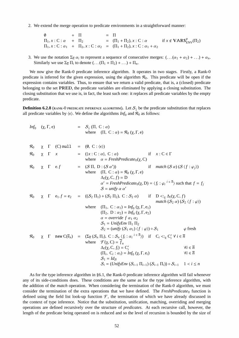
2. We extend the merge operation to predicate environments in a straightforward manner:

∅ + Π = Π

Π1, x : C : α + Π2 = (Π1 + Π2), x : C : α if x < ��PENV(Π2)

Π1, x : C : α1 + Π2, x : C : α2 = (Π1 + Π2), x : C : α1 + α2

3. We use the notationΣn αi to represent a sequence of consecutive merges: (. . . (α1 + α2) + . . .) + αn.Similarly we useΣn Πi to denote (. . . (Π1 + Π2) + . . .) + Πn.

We now give the Rank-0 predicate inference algorithm. It operates in two stages. Firstly, a Rank-0predicate is inferred for the given expression, using the algorithmR0. This predicate will be open if theexpression contains variables. Thus, to ensure that we return a valid predicate, that is, a (closed) predicatebelonging to the set��, the predicate variables are eliminated by applying a closing substitution. Theclosing substitution that we use is, in fact, the least such one: it replaces all predicate variables by the emptypredicate.

Definition 6.2.8(-0 ). LetS↓ be the predicate substitution that replacesall predicate variables by〈ǫ〉. We define the algorithmsInf0 andR0 as follows:

Inf0 (χ, Γ, e) = S↓ (Π, C : α)where (Π, C : α) = R0 (χ, Γ, e)

R0 χ Γ (C) null = (∅, C : 〈ǫ〉)

R0 χ Γ x = ({x : C : α}, C : α) if x : C ∈ Γwhere α = FreshPredicate0(χ,C)

R0 χ Γ e. f = (S Π, D : (S α′)) if match(S α) (S 〈 f : ϕ j〉)where (Π, C : α) = R0 (χ, Γ, e)

∆f (χ,C, f ) = Dα′ = FreshPredicate0(χ,D) = 〈 fi : ϕi

i ∈ n〉 such thatf = f j

S = unifyα α′

R0 χ Γ e1. f = e2 = ((S2 Π1) + (S2 Π2), C : S2 α) if D <:χ ∆f (χ,C, f )match(S2 α) (S2 〈 f : ϕ〉)

where (Π1, C : α1) = Inf0 (χ, Γ, e1)(Π2, D : α2) = Inf0 (χ, Γ, e2)α = override fα1 α2

S1 = UnifyEnvΠ1 Π2

S2 = (unify (S1 α1) 〈 f : ϕ〉) ◦ S1 ϕ fresh

R0 χ Γ new C(en) = (Σn (Sn Πi), C : Sn 〈 fi : αii ∈ n〉) if C i <:χ C′i ∀ i ∈ n

where F (χ,C) = f n∆f (χ,C, fi) = C′i ∀i ∈ n(Πi , Ci : αi) = Inf0 (χ, Γ, ei) ∀i ∈ nS1 = IdSSi = (UnifyEnv(Si−1 Πi−1) (Si−1 Πi)) ◦ Si−1 1 < i ≤ n

As for the type inference algorithm in§6.1, the Rank-0 predicate inference algorithm will fail wheneverany of its side-conditions does. These conditions are the same as for the type inference algorithm, withthe addition of thematchoperation. When considering the termination of the Rank-0 algorithm, we mustconsider the termination of the extra operations that we have defined. TheFreshPredicate0 function isdefined using the field list look-up functionF , the termination of which we have already discussed inthe context of type inference. Notice that the substitution, unification, matching, overriding and mergingoperations are defined recursively over the structure ofpredicates. At each recursive call, however, thelength of the predicate being operated on is reduced and so the level of recursion is bounded by the size of

52

the predicate. The substitution operation is technically also defined over the number of predicate variablesthat it acts upon. Thus, an argument for the termination of the substitution operation will also have to takethis into account. It is clear, however, that termination isguaranteed for substitutions defined over a finitenumber of predicate variables. Moreover, the extensions ofthe unification and and merging operations topredicate environments are defined recursively over the structure of the environment itself. However, again,at each recursive call the size of the environment is reduced, and therefore the level of recursion is againbounded. Two final points to deal with are the special cases ofthe identity and closing substitutions,IdSandS↓. Formally, these are defined over the entire (infinite) set ofpredicate variables. However, in practicethey only operate on the (finite number of) predicate variables present in the predicate that they act upon.An implementation of these substitutions can then clearly be made to terminate by defining them to treatallpredicate variables that they encounter in the same manner.

We make the proposition that the Rank-0 predicate inferencealgorithm of Definition 6.2.8 is sound withrespect to predicate assignment. We also assert that it iscompletewith respect to predicate assignment usingonly Rank-0 predicates. However, due to time constraints wehave not been able to construct a proof forthis.

Conjecture 6.2.9( -0 ). If the Rank-0 inference algorithm returnsa predicate environment and a type-predicate pair for a given execution context, type environment andexpression, then there exists a predicate derivation assigning the type-predicate pair to the expression usingthe execution context and predicate environment:

χ ⊢ Γ & Inf0 (χ, Γ, e)= (Π, C : φ)⇒ Π ⊢Pχ e : C :φ

Conjecture 6.2.10( -0 ). If D::Π ⊢Pχ e : C :α such thatD containsonly Rank-0 predicates, then there exists a Rank-0 predicate α′ and a predicate substitutionS such thatR0 (χ,Π, e)= (Π′, α′) andS Π′ P Π with S α′ P α.

6.3 The Rank-1 Restriction

A restriction that precludes assigning predicates to expressions using method invocation is undoubtedlytoo severe. Method invocation is at the heart of LJ, and so a meaningful system should be able to dealwith it. For this reason, we now generalise the Rank-0 systemto be able to type expressions with methodinvocations. The Rank-1 system, however, still places restrictions of the type of method invocations thatthose expressions can contain. The methods that may be invoked are restricted to those whose bodies canbe typed with Rank-0 predicates. Thus, the Rank-1 system also cannot type expressions in which a methodis invoked on the return value of another method invocation.We first define Rank-1 predicates:

Definition 6.3.1(-1 ). 1. The set of Rank-1 predicates, denoted by��1 and rangedover byβ, is defined by the following grammar:

β F ϕ

| 〈l1 : τ1, . . . , ln : τn〉 (n ≥ 0)

τ F β

| α0::αn→ α (n ≥ 0)

Again, we say that a Rank-1 predicate isclosedwhen it does not contain any predicate variables.Also, as for closed Rank-0 predicates, the set of closed Rank-1 predicates is a subset of the set ofpredicates. Notice that��0 ⊂ ��1.

2. A Rank-1 predicate environment is a predicate environment in which the predicate conclusion of eachstatement is a Rank-1 predicate.

We must now extend the notion of predicate substitution to operate over Rank-1 predicates, as well asextend the definition of the unification, matching and overriding operations:

53

Definition 6.3.2 (-1 ). (ϕ 7→ β) : ��1 → ��1, whereϕ is a predicatevariable andβ ∈ ��1, is defined inductively as follows:

(ϕ 7→ β) ϕ = β

(ϕ 7→ β) ϕ′ = ϕ′, if ϕ′ , ϕ(ϕ 7→ β) α0::αn→ α = ((ϕ 7→ β) α0)::((ϕ 7→ β) α1), . . . , ((ϕ 7→ β) αn)→ ((ϕ 7→ β) α)(ϕ 7→ β) 〈l i : τi

i ∈ n〉 = 〈l1 : (ϕ 7→ β) τ1, . . . , ln : (ϕ 7→ β) τn〉

This extends to Rank-1 predicate environments in a similar way as for Rank-0 substitution (see Definition6.2.2).

We now present modifications to the unification, matching andmerging operations so that they canhandle Rank-1 predicates. The extensions are straightforward and minor, amounting to extra cases in eachoperation for handling method predicate types, and generalising the cases for object predicates so that theymay contain both field identifiers and method names. We do not give the extension for the override operation,since the definition is identical to the Rank-0 version, except that Rank-1 predicates are used instead ofRank-0 ones.

Definition 6.3.3(). Unification is defined over Rank-1 predicates by:

unify ϕ β = (ϕ 7→ β)unify 〈l i : τi

i ∈ n〉 ϕ = unifyϕ 〈l i : τii ∈ n〉

unify α0::αn→ α α′0::α′n→ α′ = S ◦ Sn ◦ . . . ◦ S0

whereS = unifyα α′

Si = unifyαi α′i for all 0 ≤ i ≤ n

unify 〈ǫ〉〈l i : τii ∈ n〉 = IdS

unify 〈l : τ〉〈ǫ〉 = IdS

unify 〈l : τ〉〈l′ : τ′〉 =

{unify τ τ′ if l = l′

IdS otherwise

unify 〈l : τ〉〈l i : τii ∈ n〉 = unify (S 〈l : τ〉) (S 〈l i : τi

i ∈ n−1〉) if n > 1whereS = unify 〈l : τ〉〈ln : τn〉

unify 〈l i : τii ∈ n1〉〈l′i : τ′i

i ∈ n2〉 = S2 ◦ S1 if n1 > 1whereS1 = unify 〈ln : τn〉〈l′i : τ′i

i ∈ n2〉

S2 = unify (S1 〈l i : τii ∈ n1−1〉) (S1 〈l′i : τ′i

i ∈ n2〉)

This modification extends to theUnifyEnvfunction in the same way as the Rank-0 version. The definitionis identical, but for the obvious fact that the Rank-1unify is used.

Definition 6.3.4(). We extend thematchoperation as follows:

match ϕ ϕ′ =

{ if ϕ = ϕ′

otherwise

match α0::αn→ α α′0::α′n→ α′ = matchα α′ ∧matchα0 α′0 ∧

. . . ∧matchαn α′n

match 〈l i : τii ∈ n〉〈ǫ〉 =

match 〈l i : τii ∈ n〉〈l : τ〉 =

{ if ∃ j ∈ n [l = l j & matchτ j τ] otherwise

match 〈l i : τii ∈ n1〉〈l′i : τ′i

i ∈ n2〉 = match〈l i : τii ∈ n1〉〈l′n : τ′n〉

∧match〈l i : τii ∈ n1〉〈l′i : τ′i

i ∈ n2−1〉

54

Definition 6.3.5 ( ). The predicate merge operation is extended to Rank-1 predicates asfollows:

ϕ + ϕ′ = ϕ if ϕ = ϕ′

α0::αn→ α + α′0::α′n→ α′ = (α0 + α′0)::(α1 + α

′1), . . . , (αn + α

′n)→ (α + α′)

〈ǫ〉 + 〈l i : τii ∈ n〉 = 〈l i : τi

i ∈ n〉

〈l : τ〉 + 〈l i : τii ∈ n〉 =

{〈l1 : τ1, . . . , l j : τ + τ j , . . . , ln : τn〉 l = l j

〈l : τ〉 ⊔ 〈l i : τii ∈ n〉 l < ln

〈l i : τii ∈ n〉 + 〈l′i : τ′i

i ∈ n〉 = 〈l i : τii ∈ n−1〉 + (〈ln : τn〉 + 〈l′i : τ′i

i ∈ n′〉)wheren > 1

This definition of merging extends to Rank-1 predicate environments in exactly the same way as the Rank-0merge operation does. We also retain theΣn notation.

The extension of theFreshPredicate0 function is also straightforward. To generate a fresh Rank-1 pred-icate, we must also include the (Rank-1) methods for the given class.

Definition 6.3.6 ( (-1)). The functionFreshPredicate1 : �� × ��C →

��1 returns a Rank-1 predicate containing all fields in a given class C, with each field associated witha fresh predicate variable. It also contains all methods belonging to the class with member predicatesconstructed from fresh variables:

FreshPredicate0(χ,C) = 〈 fi : ϕii ∈ n1〉 ⊔ 〈mi : τi

i ∈ n2〉

where F (χ,C) = f n1ϕn1

freshM(χ,C) = mn2

∆m(χ,C,m) = Cini → Ci ∀ i ∈ n2

τi = ϕ0::ϕni→ ϕ ϕ, ϕ0, ϕni

fresh ∀ i ∈ n2

Note that this construction assumes that all the methods belonging to the class can be assigned Rank-1predicates. This does not present a particular problem, however, since such fresh Rank-1 predicates will onlybe generated as part of a variable predicate. Then, the algorithm simply asserts that given an environmentin which the variable satisfies such a predicate, the final result is valid. Any predicate inferred for an objectconstructed via anew expression will contain only those methods whose bodiescanbe typed with a Rank-0predicate. We do not perform this check for variables since variables may represent objects of asubtypeoftheir decared type. Therefore, we cannot be sure which method body will actually be executed when themethod is invoked on an object substituted for the variable.

We must now define one extra operation on Rank-1 predicates before presenting the Rank-1 predicateinference algorithm itself. This operation is that offlattening, or converting a Rank-1 predicate into a Rank-0 predicate by discarding all the information regarding methods. This operation is necessary when definingthe case for method invocation in the predicate inference algorithm. In the full predicate assignment system,as well as having a method predicate type, the receiver of a method invocation must also satisfy the selfpredicate of that method type. Since, in the Rank-1 system, the self predicate must be Rank-0, the algorithmtakes the Rank-1 predicate that has been inferred for the receiver expression, and flattens it before matchingit against the self predicate of its inferred method type.

Definition 6.3.7 ( ). If β is a Rank-1 predicate, then we define the flattening operation,⌊β⌋, which returns a Rank-0 predicate, as follows:

⌊ϕ⌋ = ϕ

⌊〈ǫ〉⌋ = 〈ǫ〉

⌊〈 f : β〉⌋ = 〈 f : ⌊β⌋〉⌊〈m : α0::αn→ α〉⌋ = 〈ǫ〉

⌊〈l i : τii ∈ n〉⌋ = ⌊〈l i : τi

i ∈ n−1〉⌋ ⊔ ⌊〈ln : τn〉⌋

55

We now present the Rank-1 predicate inference algorithm. The major differences between this algorithmand the Rank-0 algorithm are the extra case for method invocation, and an extension of the case for objectcreation in which types for its (Rank-0) methods are also inferred as well as fields.

Definition 6.3.8 (-1 ). Again, letS↓ be the subsitution that replaces all predicatevariables with〈ǫ〉. We define the algorithmsInf1 andR1 as follows:

Inf1 (χ, Γ, e) = S↓ (Π , C: β)where (Π, C : β) = R1 (χ, Γ, e)

R1 χ Γ (C) null = (∅, C : 〈ǫ〉)

R1 χ Γ x = ({x : C : β}, C : β) if x : C ∈ Γwhere β = FreshPredicate1(χ,C)

R1 χ Γ e. f = (S Π, D : (S β′)) if match(S β) (S 〈 f : τ j〉)where (Π, C : β) = R1 (χ, Γ, e)

∆f (χ,C, f ) = Dβ′ = FreshPredicate1(χ,D) = 〈l i : τi

i ∈ n〉 such thatf = l j

S = unify β β′

R1 χ Γ e1. f = e2 = ((S2 Π1) + (S2 Π2), C : S2 β) if D <:χ ∆f (χ,C, f )match(S2 β) (S2 〈 f : ϕ〉)

where (Π1, C : β1) = Inf1 (χ, Γ, e1)(Π2, D : β2) = Inf1 (χ, Γ, e2)β = override f β1 β2

S1 = UnifyEnvΠ1 Π2

S2 = (unify (S1 β1) 〈 f : ϕ〉) ◦ S1 ϕ fresh

R1 χ Γ e0.m(en) = ((S Π0) + Σn (S Πi), D : S ϕ) if C i <:χ C′i ∀ i ∈ n,match(S β) (S 〈m : ϕ0::ϕn→ ϕ〉),match(S ⌊β⌋) (S ϕ0),match(S αi) (S ϕi) ∀ i ∈ n

where (Π0, C0 : β) = R1 (χ, Γ, e0)(Πi , Ci : αi) = R0 (χ, Γ, ei) ∀ i ∈ n∆m(χ,C0,m) = C′n→ DS0 = UnifyEnvΠ0 Π1

Si = (UnifyEnv(Si−1 Πi) (Si−1 Πi+1)) ◦ Si−1 1 ≤ i < nSn = (unify (Sn−1 β) (Sn−1 〈m : ϕ0::ϕn→ ϕ〉)) ◦ Sn−1 ϕ, ϕ0, ϕn freshS′0 = (unify (Sn ⌊β⌋) (Sn ϕ0)) ◦ Sn

S′i = (unify (S′i−1 αi) (S′i−1 ϕi)) ◦ S′i−1 ∀ i ∈ nS = (unify (S′n ϕ) FreshPredicate0(χ,D)) ◦ S′n

R1 χ Γ new C(en) = (Σn (Sn Πi), C : (Sn 〈 fi : βii ∈ n〉) ⊔ 〈mi : αi

0::αini → αi

i ∈ n′〉)

if C i <:χ C′i ∀ i ∈ n, C′′j <:χ C j ∀ j ∈ n′

where F (χ,C) = f n,M(χ,C) = mn′

∆f (χ,C, fi) = C′i ∀i ∈ n(Πi ,Ci : βi) = Inf1 (χ, Γ, ei) ∀i ∈ nS1 = IdSSi = (UnifyEnv(Si−1 Πi−1) (Si−1 Πi)) ◦ Si−1 1 < i ≤ n

∆m(χ,D,mi) = Cini → Ci ∀ i ∈ n′

(χ,D,mi) = (xni , e′i ) ∀ i ∈ n′

Γi = {xi1 : Ci

1, . . . , xini

: Cini, this : D} ∀ i ∈ n′

(Π′i , C′′i : αi) = R0 (χ, Γi , e′i ) ∀ i ∈ n′

such that xi1 : Ci

1 : αi1, . . . , x

in1

: Cin1

: αin1, this : D : αi

0 ∈ Π′i ∀ i ∈ n′

56

As for type inference and Rank-0 predicate inference, we nowturn our attention to the termination ofthe Rank-1 predicate inference algorithm. Firstly, noticethat the extensions to the substitution, unification,matching and merging operations are such that they are stilldefined recursively over the structure of (Rank-1) predicates with each recursive call reducing the size of the predicate. It therefore remains the case thatthey are terminating over finite predicates. This argument also applies to the newly definedflatteningoper-ation. TheFreshPredicate1 function is extended to create Rank-1 predicates (i.e. predicates with memberstatements about methods as well as fields), and so is defined using the method list look-up function. How-ever, in the same way that the field list look-up function is terminating (see the discussion in§6.2), we cansee that the method list look-up function is also terminating. Lastly, a similar argument holds for themethodbodylook-up function,, which is used in the case for method invocation in the main algorithm.

Again, we make the proposition that Rank-1 predicate inference issound, and also that it iscompletewith respect to predicate assignment using only Rank-1 predicates:

Conjecture 6.3.9( -1 ). If the Rank-1 inference algorithm returnsa predicate environment and a type-predicate pair for a given execution context, type environment andexpression, then there is a predicate derivation assigningthe type-predicate pair to the expression using theexecution context and predicate environment:

χ ⊢ Γ & Inf1 (χ, Γ, e)= (Π, C : φ)⇒ Π ⊢Pχ e : C :φ

Conjecture 6.3.10( -1 ). If D::Π ⊢Pχ e : C :β such thatD containsonly Rank-1 predicates, then there exists a Rank-1 predicate β′ and a predicate substitutionS such thatR1 (χ,Π, e)= (Π′, β′) andS Π′ P Π with S β′ P β

57

Chapter 7

Conclusions and Future Work

We have developed a formal model of a class-based object oriented programming language, inspired byother similar calculi. The motivation for doing this was to demonstrate that an intersection type assignmentsystem can be applied to the class-based flavour of the objectoriented paradigm, as well to the object-based variety. We have indeed shown that this is possible by taking the predicate system of van Bakel andde’Liguoro, as described in [5], and modifying it to apply toour calculus, LJ. We have demonstrated thesuccess of this approach by proving subject reduction and expansion theorems.

Our calculus was inspired by two previous efforts: Featherweight Java and Middleweight Java. It incor-porates features from both systems, although it is closer innature to the former. Both Featherweight Javaand our calculus, LJ, are functional in nature, while MJ describes a number of imperative features. Thismakes our calculus a great deal less complex that MJ, howeverit does mean that we have not been able toinvestigate how the intersection type system interacts with imperative features. We note that this is not afeature of the system in [5] either.

We feel that LJ, even though it is very similar to Featherweight Java, is more elegant than that calculus.We have chosen to omit casts from our system, and in doing so have avoided complications in provingsubject reduction. Additionally, the reduction of LJ cannot become stuck with ‘class cast exceptions’ (stupidcasts) in the way that FJ expressions can. We have also added null objects and field assignment capabilitiesto our calculus with what we feel is very little additional complexity.

We have also examined the characterisation capabilities ofthe predicate system that we have defined forLJ. We have seen that convergent expressions are characterised by the assignability of non-trivial predicates,and we have also seen how expressions that can be assigned non-trivial predicates will not result in ‘nullreference exceptions’. Although not rigorously proved, wehope the reader is convinced that such propertiesare likely to hold, given the similarities between our system, and the intersection type systems for theLambda Calculus. Finally, we have defined two restrictions to the predicate assignment system that weassert are decidable.

There are many directions that future research in this area could go. A number of extensions are im-mediately obvious. Firstly the soundness and completenessof the Rank-0 and Rank-1 predicate inferencealgorithms remain to be proven. A general definition for a Rank-n restriction would also be useful. Anotherpossible avenue of investigation that would further cementthe theoretical foundations of the class-basedobject oriented paradigm is to define an encoding of the Lambda Calculus in LJ. This has been done for theς-calculus in [1], and would demonstrate the expressive power and equivalence of LJ with theλ-calculus.On a broader note, semantic models for LJ, as well as other class-based calculi, could be developed. [5]addresses this issue for theς-calculus, so it seems likely that a similar approach could be taken for LJ.

We have discussed above how LJ lacks imperative features, such as the ones expressed in MJ. A furtherstep might be to add these features to LJ, and also extend the predicate system to handle them. It would beinteresting to see if they can easily subsumed into the predicate system, or whether the presence of side-effects will necessitate more drastic changes. Taking anotherlead from [8], we could also incorporate aneffects system into our calculus. Again, one would hope that this extension would dovetail easily with thepredicate system.

59

Bibliography

[1] M. Abadi and L. Cardelli.A Theory Of Objects. Springer-Verlag New York, Inc., Secaucus, NJ, USA,1996.

[2] S. van Bakel. Intersection Type Assignment Systems.Theoretical Computer Science, 151(2):385–435,1995.

[3] S. van Bakel. Rank 2 Intersection Type Assignment in TermRewriting Systems.Fundamenta Infor-maticae, 2(26):141–166, 1996.

[4] S. van Bakel. Cut-Elimination in the Strict Intersection Type Assignment System is Strongly Normal-ising. Notre Dame Journal of Formal Logic, 45(1):35–63, 2004.

[5] S. van Bakel and U. de’Liguoro. Logical Equivalence for Subtyping Object and Recursive Types.Theory of Computing Systems, 42(3):306–348, 2008.

[6] H. Barendregt.The Lambda Calculus, Its Syntax and Semantics. North-Holland, Amsterdam, 1981.

[7] H. Barendregt, M. Coppo, and M. Dezani-Ciancaglini. A Filter Lambda Model and the Completenessof Type Assignment.Journal of Symbolic Logic, 48(4):931–940, 1983.

[8] G. Bierman, M. J. Parkinson, and A. Pitts. MJ: An Imperative Core Calculus for Java and Java withEffects. Technical Report 563, University of Cambridge Computer Laboratory, 15 JJ Thompson Ave.,Cambridge, CB3 0FD, UK, April 2003.

[9] A. Church and J. B. Rosser. Some Properties of Conversion. Transactions of the American Mathemat-ical Society, 39:472–482, 1936.

[10] M. Coppo and M. Dezani-Ciancaglini. An Extension of theBasic Functionality Theory for theλ-Calculus.Notre Dame, Journal of Formal Logic, 21(4):685–693, 1980.

[11] M. Coppo, M. Dezani-Ciancaglini, and B. Venneri. Functional Characters of Solvable Terms.Zeitschrift fur Mathematische Logik und Grundlagen der Mathematik, 27:45–58, 1981.

[12] H. B. Curry and R. Feys.Combinatory Logic, volume 1. North-Holland, Amsterdam, 1958.

[13] O-J. Dahl and K. Nygaard. SIMULA: an ALGOL-based Simulation Language. Commun. ACM,9(9):671–678, 1966.

[14] S Drossopoulou and S Eisenbach. Is The Java Type System Sound. InIn Proceedings of the FourthInternational Workshop on Foundations of Object-OrientedLanguages, 1997.

[15] M. Flatt, S. Krishnamurthi, and M. Felleisen. Classes and Mixins. In In Principles of ProgrammingLanguages (POPL, pages 171–183. ACM Press, 1998.

[16] A. Goldberg and D. Robson.Smalltalk-80: The Language and its Implementation. Addison-WesleyLongman Publishing Co., Inc., Boston, MA, USA, 1983.

[17] J. Gosling, B. Joy, G. Steele, and G. Bracha.The Java Language Specification (3rd Edition). PrenticeHall, 2005.

61

[18] A. Igarashi, B. Pierce, and P. Wadler. Featherweight Java: A Minimal Core Calculus for Java and GJ. InACM SIGPLAN Conference on Object Oriented Programming: Systems, Languages, and Applications(OOPSLA), October 1999. Full version in ACM Transactions on Programming Languages and Systems(TOPLAS), 23(3), May 2001.

[19] R. Milner, M. Tofte, R. Harper, and D. MacQueen.The Definition of Standard ML (Revised). MITPress, 1997.

[20] T. Nipkow and D. von Oheimb. Javalight Is Type-Safe—Definitely. InPOPL ’98: Proceedings of the25th ACM SIGPLAN-SIGACT symposium on Principles of programming languages, pages 161–170,New York, NY, USA, 1998. ACM.

[21] Microsoft Press.C# Language Specifications. Microsoft Press, U.S., May 2001.

[22] J. A. Robinson. A Machine-Oriented Logic Based on the Resolution Principle.J. ACM, 12(1):23–41,1965.

[23] B. Stroustrup.The C++ Programming Language, Second Edition. Addison-Wesley, 1991.

[24] A. M. Turing. Computability and Lambda-Definability.J. Symb. Log., 2(4):153–163, 1937.

62

intersection types for class-based object oriented programming · intersection type systems have...

Documents