IZA DP No. 2924

Interprovincial Migration in China:The Effects of Investment and Migrant Networks

Shuming BaoÖrn B. BodvarssonJack W. HouYaohui Zhao

DI

SC

US

SI

ON

PA

PE

R S

ER

IE

S

Forschungsinstitutzur Zukunft der ArbeitInstitute for the Studyof Labor

July 2007

Interprovincial Migration in China:

The Effects of Investment and Migrant Networks

Shuming Bao University of Michigan

Örn B. Bodvarsson

St. Cloud State University and IZA

Jack W. Hou

California State University, Long Beach

Yaohui Zhao Beijing University

Discussion Paper No. 2924 July 2007

IZA

P.O. Box 7240 53072 Bonn

Germany

Phone: +49-228-3894-0 Fax: +49-228-3894-180

E-mail: iza@iza.org

Any opinions expressed here are those of the author(s) and not those of the institute. Research disseminated by IZA may include views on policy, but the institute itself takes no institutional policy positions. The Institute for the Study of Labor (IZA) in Bonn is a local and virtual international research center and a place of communication between science, politics and business. IZA is an independent nonprofit company supported by Deutsche Post World Net. The center is associated with the University of Bonn and offers a stimulating research environment through its research networks, research support, and visitors and doctoral programs. IZA engages in (i) original and internationally competitive research in all fields of labor economics, (ii) development of policy concepts, and (iii) dissemination of research results and concepts to the interested public. IZA Discussion Papers often represent preliminary work and are circulated to encourage discussion. Citation of such a paper should account for its provisional character. A revised version may be available directly from the author.

IZA Discussion Paper No. 2924 July 2007

ABSTRACT

Interprovincial Migration in China: The Effects of Investment and Migrant Networks*

Since the 1980s, China’s government has eased restrictions on internal migration. This easing, along with rapid growth of the Chinese economy and substantial increases in foreign and domestic investments, has greatly stimulated internal migration. Earlier studies have established that migration patterns were responsive to spatial differences in labor markets in China, especially during the 1990s. However, other important economic and socio-political determinants of interprovincial migration flows have not been considered. These include the size of the migrant community in the destination, foreign direct and domestic fixed asset investments, industry and ethnic mixes and geographic biases in migration patterns. We estimate a modified gravity model of interprovincial migration in China that includes as explanatory variables: migrant networks in the destination province, provincial economic conditions, provincial human capital endowments, domestic and foreign investments made in the province, industry and ethnic mixes in the province, provincial amenities and regional controls, using province-level data obtained from the National Census and China Statistical Press for the 1980s and 1990s. We find strong evidence that migration rates rise with the size of the destination province’s migrant community. Foreign and domestic investments influence migration patterns, but sometimes in unexpected ways. We find that as economic reforms in China deepened in the 1990s, the structure of internal migration did not change as much as earlier studies have suggested. Consequently, our results raise new questions about the World’s largest-scale test case of internal migration and strongly suggest a need for further research. JEL Classification: J61 Keywords: internal migration, investment, migrant networks Corresponding author: Örn B. Bodvarsson Department of Economics St. Cloud State University 720 Fourth Avenue South St. Cloud, MN 56301 USA E-mail: obbodvarsson@stcloudstate.edu * We thank Gewei Wang and Robert Girtz for assistance in the assembly of our data set and bear full responsibility for any errors.

3

I. INTRODUCTION

For researchers studying internal migration in transition economies, China is a

tremendously valuable natural experiment. Since the 1980s, there has been a gradual

easing of restrictions on internal migration in China.1 During the same period, several

broad comprehensive market reforms2, globalization and large infusions of foreign direct

investment all created considerable prosperity in China but also contributed to significant

interregional income inequality. Consequently, China experienced a surge in internal

migration between the 1980s and 1990s. Based on the 1% population sample survey of

1 For those not familiar with the migration-related policy changes in China, between 1949 and 1978

migration within China was very strictly controlled by the government’s hukou system, a household

registration system that was designed to directly regulate population redistribution, as well as to provide the

government with a mechanism for gathering population statistics and to identity personal status. Under the

hukou system, households had to register with the government, the government assigned persons jobs and

rationed living necessities in urban areas. If a person wanted to move, approval had to be obtained from

his/her local government. Consequently, intra- and interprovincial migration were rare, except for situations

involving “planned” migration from the Eastern parts of the country to the much less-populated Western

areas during the Cultural Revolution period of the 1960s and 1970s. Since 1978, when the government

initiated the Comprehensive Economic Reform (CER) program, the hukou system has been incrementally

dismantled. The first step towards dismantling came with the introduction of identity cards in the late

1980s, which allowed persons to travel around China without showing an official “permission” letter from

his/her local government. The next step was the abolition of grain rationing coupons in the early 1990s;

these coupons were the means by which people obtained food rations and they could only be used in the

place of residence. With the abolition of the coupons, individuals were free to obtain food where they

wished. A third step occurred in 2001, when residency in small towns and townships was open to all rural

workers who were legally employed and had a place to live. At roughly the same time, medium-sized cities

and some provincial capitals eliminated ceilings on the number of rural workers who could apply for

permanent residence status. Some very large cities such as Shanghai and Beijing concurrently eased

restrictions on the in-migration of rural workers. 2 The first reform was the decollectivization of agriculture (also known as the inception of the household

responsibility system) in rural areas. The most important aspect of this reform is that it freed workers to

choose how they wanted to allocate their labor supplies. This encouraged many workers to leave the

agricultural sector and seek employment in other sectors, most notably enterprises in urban areas. The

second consisted of a set of market-oriented reforms in the urban areas during the late 1980s. The

government, in an effort to attract foreign direct investment, created favorable provisions, e.g. tax

concessions and attractive terms for leasing land, to many coastal cities so they could establish economic

development areas and high technology development zones. In the 1990s, the government gave special tax

and regulatory treatment to certain areas (called “special economic zones”), which generated large amounts

of FDI in those areas. These economic reforms had the effect of creating large real income differentials

between the Eastern provinces and the rest of China, encouraging Eastward migration.

4

1987, it is estimated that over 30 million Chinese relocated either within or between

provinces during 1982-87. Using data from the 2000 Chinese Census, researchers have

estimated that intra- and interprovincial migration during 1995-2000 totaled over 144

million persons, or about 12% of average provincial population during that period. Much

of the surge in migration involved rural residents moving to urban areas, particularly the

metropolitan coastal cities and Beijing.

Prior to 1987, research on internal migration in China was severely hampered because

national level data on internal migration was generally non-existent. The first national

survey that included questions about migration was the 1987 1% population survey and

1990 was the first year in which the government collected data on migration in the

population census. The 1990 census asked questions about both inter- and intra-

provincial migration for the period 1985-90 and the 2000 census included questions about

migration during 1995-2000. There have also been a number of household surveys in

very specific areas of the country, which have included questions about migration.

As a result of this relatively new data on migration patterns, a small and mostly

empirical literature focusing on the determinants of internal migration in China has begun

to emerge. This literature consists of a handful of studies utilizing micro-data obtained

from special household surveys (see, for example, Liang (2001), Liang and White

(1996,1997), Zhao (1997,1999a, 1999b, 2002, 2003), Liang, Chen and Gu (2002)) and a

few studies utilizing province-level aggregate data provided by the central government

(see, for example, Lin, Wang and Zhao (2004), Poncet (2006) and Bao, Hou and Shi

(2006)). The primary objective of these studies has been to ascertain to what extent an

5

individual’s propensity to migrate (or the strength of aggregate migration flows) are

driven by regional differences in labor markets.

Among the studies that have utilized province-level aggregate data on migration

flows, the general finding has been that flows were responsive to regional differences in

income and unemployment rates during the 1980s and 1990s, controlling for other

factors, but the responsiveness of migration to changes in those rates was generally

greater during the 1990s.3 These results suggest that as Chinese economic reforms

deepened in the 1990s, the structure of internal migration changed considerably. These

studies also found that migration flows are inversely related and very sensitive to distance

between origin and destination (Lin, Wang and Zhao (2004), Poncet (2006), Bao, Hou

and Shi (2006)) and domestic trade barriers (Poncet (2006)), positively related to the

destination population’s level of educational attainment4 (Lin, Wang and Zhao (2004))

and responsive to regional differences in climate (Lin, Wang and Zhao (2004)), the

agricultural industry’s share of provincial employment (Bao, Hou and Shi (2006)) and the

share of the destination province’s population consisting of persons belonging to minority

groups (Bao, Hou and Shi (2006)).

In this study, we contribute to ongoing research on the determinants of interprovincial

migration flows in China by examining several fundamental determinants not examined

3 For example, Lin, Wang and Zhao (2004), using 1990 and 2000 Census data on interprovincial migrant

flows, found that after controlling for distance, relative educational attainment, relative unemployment

rates, the relative degree of urbanization and climatic differences, migration did not respond to income

differences during 1985-90, but was relatively sensitive to those differences during 1995-2000. Poncet

(2006), utilizing both Chinese Census data from 1990 and 2000 and 1995 National Population Survey data,

found that migration was responsive to regional income differences during the 1980s and 1990s, but the

responsiveness was greater in the later period. Both studies attribute the greater sensitivity of

interprovincial migration to spatial differences in income during the later period to the significant reduction

in migration barriers that occurred during that period. Both these studies measured income as mean per

capita income in each province, obtained from the National Bureau of Statistics. In contrast, however, Bao,

Hou and Shi (2006), using data on per capita GDP to proxy provincial income per capita, found that during

the 1990s there was actually no relationship between income and interprovincial migration flows. 4 Only for the 1990s, however.

6

in earlier studies. The first is the size of the migrant community in the destination. Many

studies on both internal and international migration have confirmed that current flows of

migrants from place i to place j are often strongly influenced by the number of persons

residing in j who previously migrated from i. These are often called “kinship” or

“network” effects on migration; the presence of friends, family and other contacts already

at the destination tends to lower the psychic and information costs generated by

migration. Zhao (2003) examined the influence of migrant networks on Chinese internal

migration using micro-level household survey data from a very specific location in rural

China and found that experienced migrants have a positive and significant effect on

subsequent migration, although return migrants apparently have no effect. One of the

goals of our study is to ascertain whether Zhao’s results are generalizable to all of China

through a study utilizing aggregate data on province-to-province migration flows.

A second factor we contend will influence migration is investment spending in the

province, specifically domestic fixed asset investment (which consists primarily of

residential and commercial construction spending) and foreign direct investment (FDI).

Between the 1980s and 1990s, there have been substantial increases in both types of

investment spending in most of the provinces. According to the China Statistical Press,

mean annual per capita FDI in each province soared from US$3.14 during 1985-90 to

US$44.62 during 1995-2000. Much of this increase went to specific areas in the country

designated by the government to receive special treatment with respect to economic

development. According to the same source, mean annual fixed asset investment per

capita in each province rose from 89 Yuan during 1985-90 to 247 Yuan during 1995-

2000. We hypothesize that higher investment spending in a province will induce

7

“demand-pull” migration; greater spending on infrastructure, for example, will increase

the demand for labor, including migrant labor. Liang and White (1997) tested for the

effects of province-level foreign investment on the likelihood of an individual migrating

from the province using data taken from a 10% random sample of the China 2/1,000

Fertility and Birth Control Survey, and found no evidence of such effects. We contend

that any effects of FDI or domestic fixed asset investment spending on migration

decisions are much more likely to be observed in aggregate data, as opposed to micro-

data sets obtained from household surveys in very small parts of the country. One goal of

this study is to examine the relationship between aggregate migration flows and both

types of investment.

We also consider the possible influences of industry and ethnic mixes in the province

and regional biases in migration patterns. We hypothesize that the extent of emigration

will be influenced by the dominance of manufacturing in the destination province relative

to the origin province, as well as the dominance of the minority population (which was

also examined by Bao, Hou and Shi (2006)). Furthermore, we control for region of

destination in order to ascertain whether, all other things equal, there were greater

tendencies for Westward or Eastward migration.

The remainder of this paper is organized as follows. In the next section, we present

a version of a modified gravity regression model of interprovincial migration flows,

followed by a discussion of our data set and then empirical results obtained from OLS

estimation. The final section discusses implications for future research.

8

II. THE DETERMINANTS OF INTERPROVINCIAL MIGRATION ;

THEORY and EMPIRICAL SPECIFICATION

We estimate a version of the traditional modified gravity model of internal migration,

which is applied here to the case of interprovincial migration in a developing country

experiencing substantial market reforms.5 Unique to this version is the inclusion of

provincial investment and migrant network controls, as well as other controls for a

province’s economic, political and social characteristics. The dependent variable is the

log of the gross interprovincial emigration rate in period t (log(Mijt)), calculated as the

volume of out-migration from province i to province j during the period divided by total

interprovincial migration from province i during that period. The equation to be

estimated is

(1) log Mijt = α0 + α1logDij + α2logNETWORKijt + α3logFDI(i)(t-k) + α4logFDI(j)(t-k) +

α5logINV(i)(t-k) + α6logINV(j)(t-k) + α7(logINV(i)(t-k))(logFDI(i)(t-k)) +

α8(logINV(j)(t-k))(logFDI(j)(t-k)) + α9logYit + α10logYjt + α11logEit + α12logEjt + α13logUit +

α14logUjt + α15logMANUit + α16logMANUjt + α17logMINit + α18logMINjt + α19logTit +

α20logTjt + α21NORTHWESTj + α22SOUTHWESTj + α23EASTj + α24PERIODt + εijt

where:

Dij = railway distance (in kilometers) between the capital city of province i and that of

province j;

NETWORKij = the size of the migrant community already residing in j that hails from i,

measured as the ratio of the stock of migrant residents to population;

FDI(i)(t-k), FDI(j)(t-k) = real foreign direct investment per capita spent in provinces i and j,

respectively, lagged k periods;

INV(i)(t-k), INV(j)(t-k) = real domestic fixed asset investment per capita spent in provinces i

and j, respectively, lagged k periods;

5 See Greenwood (1997, pp. 663)

9

Yi, Yj = real per capita income in provinces i and j, respectively;

Ei, Ej = mean number of years of schooling completed by residents of province i and j,

respectively, 25 years of age and above at the beginning of the period;

Ui, Uj = unemployment rates during the week preceding the implementation of the census

in province i and j, respectively;

MANUi, MANUj = proportion of provincial GDP comprising the manufacturing sector in

province i and j, respectively;

MINi, MINj = proportion of population comprising minorities in province i and j,

respectively;

Ti, Tj = mean yearly temperature in the capital city of province i and j, respectively;

NORTHWESTj = dummy variable equaling one if the destination province is one of the

Northwestern provinces;6

SOUTHWESTj = dummy variable equaling one if the destination province is one of the

Southwestern provinces;7

EASTj = dummy variable equaling one if the destination province is one of the Eastern

provinces;8

PERIODt = dummy equaling one if the observation is from the 1995-2000 period;

εij = random error term.

Railway distance and the migration rate are hypothesized to be inversely related; the

greater is distance, the greater will be the direct costs of migration (train or bus fare, food

and lodging expenses en route and upon arrival, for example) and the indirect costs of

migration (for example, lost income due to down time between employment in the origin

and employment in the destination, as well as the psychic costs of migration).

6 The Northwestern provinces include Inner Mongolia, Xinjiang, Shaanxi, Gansu and Ningxia.

7 The Southwestern provinces include Sichuan (including Chongqing), Guizhou, Yunnan, Qinghai and

Guangxi. 8 These include Beijing, Tianjin, Hebei, Liaoning, Shanghai, Jiangsu, Zhejiang, Fujian, Shandong,

Guangdong and Hainan. Note that the Central provinces include Shanxi, Jilin, Heilongjiang, Anhui,

Jiangxi, Henan, Hubei and Hunan.

10

We hypothesize that the migration rate from province i to province j will be positively

related to the size of the pre-existing migrant community in j that hails from i (the

NETWORK variable). The greater is the size of the migrant community already in the

destination, ceteris paribus the lower will be the costs of migrating because there will

tend to be more information flowing back to the origin about employment and business

opportunities, housing, schools, recreational opportunities, etc. Furthermore, there will be

lower psychic costs of migration because a larger migrant community in the destination

will tend to be a greater source of comfort, security and familiarity for those

contemplating migration.

The migration rate is hypothesized to be positively related to lagged investments in

the destination (FDI(j)(t-k) and INV(j)(t-k)) and negatively related to lagged investments in

the origin (FDI(i)(t-k) and INV(i)(t-k)). Higher investment, e.g. new commercial or residential

construction, in the destination will generate higher demand for labor from other

provinces, higher wage rates and thus an increase in “demand-pull” migration.

Conversely, higher investment in the origin will reduce the incentive to migrate from

there, all other things equal, due to more attractive labor market opportunities at home.

The two investment variables are lagged for two important reasons. First, it will very

likely take time for spending on new investment projects to result in in-migration of labor

to the area. For example, spending on new construction of apartment buildings in

Shanghai may not result in increased hiring there right away because it often takes time

for information on local labor market conditions in the destination to flow to the origin

province. Furthermore, migration is an activity that often cannot be undertaken right

away, especially if it is relatively costly and migrants must save in advance in order to

11

finance migration. Second, there is likely to be two-way causality between migration and

contemporaneous investment. On the one hand, higher current investment in the

destination may induce in-migration, but greater in-migration may itself encourage more

investment. For example, when there is a large influx of migrants to Beijing in response

to a construction boom, increased migrant demand for housing may stimulate

construction spending there.9 If investment is endogenous to migration, then a

simultaneous equations econometric model may be more appropriate. Consequently, to

avoid the need for a simultaneous equations model, we use lagged investment because it

will be exogenous to migration.

We include interactions between provincial FDI and fixed asset investment to account

for the possibility that higher levels of one type of investment may influence the

sensitivity of migration to a change in the other type. Suppose increased FDI results in

greater commercial construction spending in the destination province, stimulating in-

migration. Then the effect of the higher FDI on in-migration could be smaller the larger is

the level of fixed asset investment spending, i.e. α8 could be negative. For example,

construction firms financed by FDI may compete with firms financed internally for the

same pool of imported labor. Consequently, increased demand for migrant labor by FDI-

financed firms may induce less supply of migrant labor to those firms when there is a

higher level of fixed asset investment. By the same reasoning, the drop in out-migration

due to higher FDI in the origin province could be smaller the higher is the level of fixed

asset investment (α7 > 0).

9 FDI may also be functionally related to INV, and vice versa. If there is greater domestic fixed investment

in a city, for example, this could induce more foreign investment (especially if local authorities offer to

match foreign investment) or less foreign investment (if foreign investment is viewed as a substitute for

domestic investment).

12

The origin and destination provinces’ shares of GDP attributable to manufacturing

(MANUi and MANUj, respectively) are included as controls for industry mix in the

province. The relationship between the dominance of manufacturing in the destination

province and in-migration there is expected to be positive. Manufacturing jobs are

generally higher-skilled and higher-paying compared to, for example, jobs in the

agricultural sector. Therefore, provinces with relatively larger manufacturing sectors

should attract relatively more migrants, all other things equal, especially from provinces

that have relatively large agricultural sectors. Using the same reasoning, manufacturing’s

share of output in the origin province should be negatively related to out-migration from

that province.

Following Bao, Hou and Shi (2006, pp. 335), we include a control for the relative

proportion of the destination’s population that is minority.10

We include this variable for

several reasons and postulate that its effect on migration could be positive or negative.

First, this variable may proxy general political conditions in the province, e.g. provinces

with larger minority population shares may have more political divisiveness than other

provinces, which may influence migration patterns. Second, there are several economic

reasons why the minority population share may influence migration. As Bao, Hou and

Shi (2006) point out, provinces with relatively large minority population shares tend to

lack many basic service industries, hence entrepreneurial migrants seeking to start service

businesses may find these provinces profitable places to relocate to. On the other hand,

professionals seeking salaried positions may be less interested in migrating to provinces

10

The proportion of a province’s population that is minority was computed in the following way:

.100)population total

populationHan - population total( minority of % x

13

with higher minority shares because they may perceive such provinces to have more

limited high-skill employment opportunities.

The NORTHWEST, SOUTHWEST, EAST, and PERIOD controls are included to

account for regional and period differences in migration. During the 1980s and part of the

1990s, Eastern China, particularly the coastal cities, experienced considerable prosperity

relative to the West. This has been cited as a major factor for substantial Eastward

migration during that period. Accordingly, the Western sub-regional dummies are

included as controls for any ceteris paribus regional bias for or against migration to the

Western part of China. The EAST dummy is included as a control for regional bias in

migration for or against the Eastern part of the country. The PERIOD variable is included

as a general control for increased deregulation of migration during the later period.

Following the earlier literature on internal migration, we hypothesize that migration

rates will be positively related to real relative income in the destination (Yj), since the

returns to migrating will be higher the greater is the real relative return to supplying one’s

labor services in the destination. Conversely, we hypothesize a negative relationship

between the rate of migration and real income in the origin province (Yi). The migration

rate is hypothesized to be positively related to the average level of educational attainment

in the destination (Ej) because the existence of a better educated labor force there usually

means a distribution of higher quality employment opportunities. However, using the

same type of argument, greater educational attainment in the origin (a higher value of Ei)

is hypothesized to be inversely related to the migration rate. A higher relative

unemployment rate in the destination (Uj) is expected to discourage migration, but a

higher unemployment rate in the origin (Ui) is expected to encourage migration. Relative

14

mean yearly temperature in the destination (Tj) is included as a control for destination

amenities. It is presumed that migrants prefer warmer provinces, all other things equal,

hence migration rates to warmer provinces should be higher. However, ceteris paribus

we hypothesize that migration rates out of warmer provinces will be smaller (α19 < 0).

III. DESCRIPTION OF DATA

The data set used in this study is a modified version of a data set used by Lin, Wang

and Zhao (2004). Lin, Wang and Zhao graciously shared their data set with us and we

used most of it without any modifications. However, there are ten provincial data series

included in our data set not found in Lin, Wang and Zhao’s data set. First, we replaced

their interprovincial migration rate series with our own. The reason is that there are some

inaccuracies in the series used by Lin, Wang and Zhao, which they acknowledged in

some very recent communications with us. Second, we added nine new variables -- the

pre-existing migrant community in the destination, real FDI per capita in the origin and

destination provinces, real domestic fixed asset investment per capita in the origin and

destination provinces, the manufacturing sector’s share of GDP in the destination and

origin provinces and the minority population share in the origin and destination

provinces.

Our data set consists of 1,577 observations at the province level spanning the period

1980-2000. There are 29 provinces in our data set11

. Each of the 29 provinces was a

prospective destination and a point of origin for migration flows. Because of the log-

linear functional form for equation (1), the data set does not include any observations for

11

As with Lin, Wang and Zhao (2004), we exclude Tibet because of missing observations and treat

Chongqing as part of Sichuan.

15

which the emigration rate is zero. Equation (1) was estimated for the full sample, for the

1980s separately and then for the 1990s separately. No data were available for size of the

migrant network during the 1980s, so we estimated equation (1) without a migrant

network variable for the 1980s sub-sample (765 observations), as well as for the full

sample. However, data were available for the size of the migrant network during the

1990s, so we estimated equation (1) with and without a migrant network variable for the

1990s sub-sample. Again because of the log-linear functional form, we excluded

observations for which the migrant network was zero, leaving us with 790 observations.12

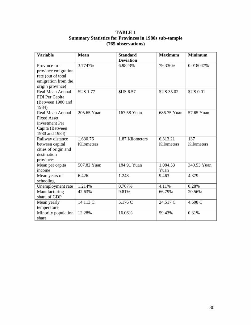
Tables 1 and 2 show summary statistics for all variables used in our regressions for

the1980s and 1990s sub-samples. Starting from the top of each table, we describe each

variable, the data source from which the variable is drawn and the trends apparent in the

data between the two periods:

(i ) Gross interprovincial migration rate. This is the number of persons migrating from

province i to province j divided by the number of persons migrating from province i.

These numbers are calculated from 1% of the 1990 population census and 0.95% of the

2000 population census13

, both sets of numbers published by the China Statistical Press.

In the 1990 (2000) census, respondents were asked to report on migration activities

12

Note that while the full sample is 1,577 observations, the sum of the two subsamples is 1,555

observations. The reason is that in the full sample regression, since the migrant network variable was not

included, it was not necessary to exclude 22 observations in the 1990s subsample for which the migrant

network was zero. 13

As pointed out by Lin, Wang and Zhao, there is a small difference between the 1990 and 2000 censuses

with respect to how migration is defined. If a person is observed to change residence and to change their

household registration (a situation called hukou migration), then this movement as classified as “migration”

in both censuses. If, however, the person is observed to change residence without changing registration (the

case of non-hukou migration), then the movement is classified as “migration” only if the migrant has been

away from the place of registration for a minimum period of time. In the 2000 census, this period is 6

months, but in the 1990 census it is one year. To account for this change in classification between the two

periods, the migration numbers in both periods were standardized by discounting the 2000 numbers by a

small amount, approximately 5%. For further details, see Lin, Wang and Zhao (2004, page 593).

16

during 1985-90 (1995-2000). Consequently, migration rates during each decade were

calculated for the second half of each decade only. The volume of migration at the

provincial level more than doubled from over 365,000 persons during 1985-90 to nearly

1,500,000 during 1995-2000.14

The surge in migration can generally be attributed to

market reforms, deregulation of the hukou system and generally rising prosperity across

the country. Note that between periods, mean provincial population rose 9.44%. For both

periods, Sichuan province experienced the highest volume of interprovincial emigration

(approximately 1,457,000 persons during 1985-90 and 4,375,000 during 1995-2000),

while Ningxia province had the lowest (approximately 54,500 persons during 1985-90

and 94,750 during 1995-2000). For the 1985-90 period, the highest migration rate was

79.34% (Guangxi to Guangdong) and the lowest was 0.02% (a tie between Jingxi to

Qinghai and Jingxi to Ningxia). During 1995-2000, the highest reported migration rate

was 87.32% (also Guangxi to Guangdong) and the lowest was 0.14% (Jingxi to Qinghai);

(ii) The size of the migrant network originally from province i that resides in province j

(NETWORK). An ideal measure of the size of a migrant network is the relative stock of

previous migrants residing in the destination province at the time the migration decision

is made. Unfortunately, unlike data sets in the USA and many European countries, such a

stock measure is not available in Chinese data sets. Therefore, we had to measure the size

of the migrant community using data on past migrant flows. There are no data on

interprovincial migrant flows prior to 1985, so our regression analyses for the 1985-90

period could not include a control for migrant network effects. However, in our

regression analyses for the 1995-2000 period, 1985-1995 migrant flows could be used to

14

There are likely to be discrepancies in the calculations of these numbers between the two decades, for

the reasons discussed in the preceding footnote.

17

proxy the size of the migrant network during 1995-2000. Consequently, we estimated the

size of the migrant community residing in province j that hails from province i in 2000 by

taking the ratio of migration from i to j during 1985-95 to j’s population in 2000. The

assumption underlying these calculations is that the stock of previous migrants is

proportional to the size of the previous flow of migrants. While not an ideal measure, we

are confident that data on flows over a longer (10-year) period should be relatively

accurate. Note from Table 2 that the average size of the migrant community in each

province is approximately 25,000 persons;

(iii) Lagged real annual FDI per capita in the province. FDI data were obtained from the

China Statistical Press. For each period, we used mean annual real FDI per capita, as well

as mean annual real fixed asset investment per capita, during 1980-84 when regressing

1985-90 migration flows and 1990-94 when regressing 1995-2000 migration flows. In

lagging investment spending this way, we are assuming that it takes on average up to 5

years for migration to respond to changes in spending on investment projects. We

adjusted the investment series for cost of living differences between the two decades, as

well as across provinces within each decade, using national government measures of

provincial CPI and calculating both series at 1985 price levels. For most of the

provinces, FDI numbers were available for each year, but for some there were missing

years. For several provinces, no investment data were available for 1980-84, so we used

the earliest year available as a proxy for that period. Therefore, our coefficient estimates

for the early period may be influenced by measurement error in parts of the investment

series. Note that the FDI series is in USA dollars, whereas the fixed asset investment

series is in Yuan.

18

Comparing Tables 1 and 2, there was a dramatic increase in FDI between the two

periods, reflecting a surge in interest by international investors in the Chinese economy

during the 1990s. In both periods, the places receiving the highest levels of FDI on a per-

person basis tended to be the main cities in China. During 1980-84, Beijing received the

most FDI ($35.02 per capita), followed by Shanghai and Guangdong province. In

contrast, Shandong received nearly zero FDI during 1980-84, followed by Gansu and

Anhui provinces. During 1990-94, however, it was Shanghai that was the largest

recipient of FDI ($50.53 per capita), whereas Qinghai province had the lowest ($0.38 per

capita).

(iv) Domestic real annual fixed investment per capita. These numbers were calculated using

the same methods as for real FDI per capita and with numbers obtained from China

Statistical Press. China experienced a dramatic increase in fixed asset investment between

the two decades, reflecting a boom in residential and commercial construction. However,

there is great disparity across provinces with respect to the level of construction spending.

During 1980-84, Shanghai experienced the highest level of fixed investment (686.75

Yuan per capita), whereas Guangxi province experienced the lowest (57.65 Yuan per

capita). During 1990-1994 Beijing experienced the highest level (approximately 1,900

Yuan per capita), whereas Guizhou experienced the lowest (approximately 160 Yuan per

capita);

(v) The manufacturing sector’s share of provincial output. These data were obtained from

the China Statistical Yearbooks. Technically, manufacturing is classified as the

“Secondary” industry in China and it includes construction as one of the components.

There is considerable variation in the dominance of the manufacturing sector across

19

China. During 1980-85, Shanghai had the highest manufacturing share (approximately

two-thirds of its GDP), whereas the lowest share was in Hainan (20.56%). During 1995-

2000, Heilongjiang province had the highest manufacturing share (approximately 55%),

whereas the lowest was in Hainan province (just under 21%).

(vi) The share of the province’s population that is minority. These are 2000 census data

obtained from the China Statistical Yearbooks. Because data for 1990 are not available,

we used the 2000 data to proxy minority population shares during the 1980s, as well as

during the 1990s. One can see that the minority population share varied widely across

provinces in 2000.

Data on the remaining variables are from Lin, Wang and Zhao; please refer to their paper

for details on data sources and measurement of these variables:

(vi) Mean real per capita income. Note that income data for the earlier period are for 1989

(deflated to 1985 levels), whereas for the later period are for 1999 (deflated to 1995

levels). For both periods, the highest income area was Shanghai and the lowest was

Gansu province;

(vii) Mean years of schooling. During both periods, the most well-educated population was

Beijing, whereas the lowest was Guizhou province. Note that educational attainment rose

by nearly 25% between periods, despite secondary education not being free in China;

(viii) Unemployment rates. There are considerable differences between periods in the

behavior of the unemployment rate. The unemployment rate increased dramatically in the

later period. The highest unemployment rates occurred in the metropolitan areas (Beijing

20

during 1985-90 and Shanghai during 1995-2000), whereas the lowest unemployment

rates were in Shandong (1985-90) and Yunnan (1995-2000).

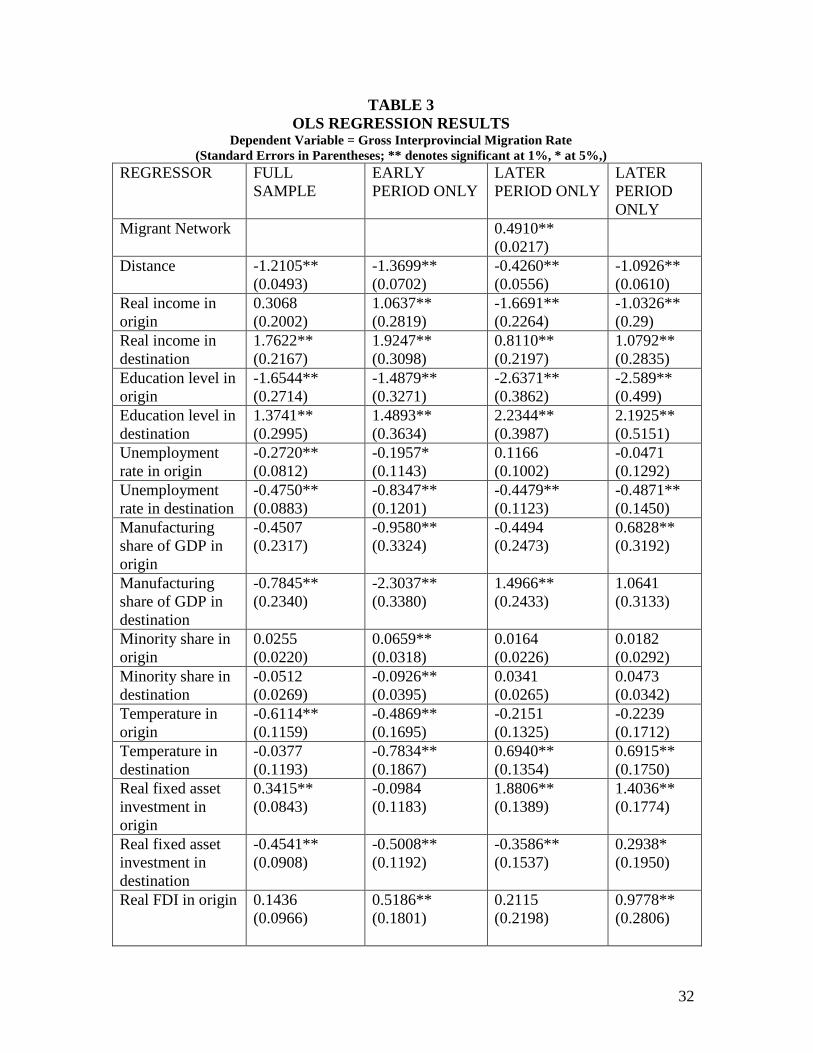
IV. EMPIRICAL RESULTS

Table 3 shows OLS coefficient estimates for four different versions of equation (1).

We first estimated the equation for the full sample (migrant flows for 1985-90 and 1995-

2000 combined). We then estimated equation (1) separately for each period. Note that the

full sample and 1980s-only regressions do not include the migrant network variable

(NETWORK) due to absence of data on pre-1985 migration patterns. Also, for the 1990s-

only regression, we estimated two equations – one with the migrant network variable and

one without.

Starting from the top row of the table, we find very strong evidence of a “migrant

network” effect; the coefficient on past migrant flows is positive and significant at better

than 1% and predicts that a 1% increase in the size of the destination province’s pre-

existing community of migrants hailing from the origin province will, all other things

equal, result in the rate of migration being higher by approximately 0.5%. This supports

the general hypothesis that larger migrant networks encourage migration because they

lead to lower informational and psychic costs of migration.

It is important to interpret the estimated coefficient on the migrant network measure in

conjunction with the estimated coefficient on railway distance, as well as in the context

of the results on railway distance obtained in Lin, Wang and Zhao’s (2004, page 597)

study. First, note that the distance coefficient is negative and significant at better than

1% for all four regressions. For example, in the regression conducted on the full sample,

when distance is 1% greater the interprovincial migration rate falls by over 1.2%. This is

21

consistent with theory; greater distance raises the costs of migration, direct and indirect,

and deters migration. Second, observe that the distance coefficient is much less negative

in the later period regression when the migrant network variable is included. In fact, our

coefficients for distance in the full sample and early period regressions are similar to the

coefficients obtained by Lin, Wang and Zhao (who did not control for migrant networks).

Lin, Wang and Zhao obtained a coefficient of -1.27% for the early period and -0.9% for

the later period. Both studies demonstrate that migration is generally less sensitive to

distance in the later period, but our study further demonstrates that the sensitivity is much

lower when a control for past migration is included.

We contend that distance and the size of the migrant network are linked by the costs

of migration; greater distance tends to increase costs, whereas a larger migrant

community in the destination tends to reduce them. We concur with Lin, Wang and Zhao

(pp. 596) that the reason their distance coefficient was less negative in the later period is

because, and we quote them, “…it is also possible that the psychic costs of migration are

declining due to the expansion of migrant networks in destinations so that long-distance

migration is less intimidating.” Lin, Wang and Zhao’s results for the distance variable

between periods likely reflect the growth in the size of the migrant network in the later

period, but also omitted variables bias. The distance variable in their regressions is likely

capturing the effects on the migration rate of an omitted migrant networks variable.

Furthermore, the reason our distance coefficient in the later period regression was much

more negative when a migrant network control was excluded is because that coefficient

reflects omitted variables bias. All this underscores the importance of including a control

for past migration when studying the determinants of internal migration.

22

Some of the estimated coefficients on the income variables are supportive of theory

and confirm that, all other things equal, a widening of the real destination/origin income

differential stimulates migration. For the later period regression which includes the

migrant network variable, for example, the estimated coefficient on origin income is

negative and significant at better than 1%, predicting that a 1% increase in income at

home will lower the out-migration rate by 1.67%. This is supportive of theory. In

contrast, for the early period regression we predict that a 1% increase in origin income

will, all other things equal, induce a 1.06% increase in the out-migration rate. That result

is not supportive of theory. The coefficients on destination income across all four

regressions are all consistent with theory and are significant at better than 1%. For the full

sample, the coefficient predicts that a 1% increase in real per capita income in the

destination will raise the in-migration rate by 1.76%. Note, however, that in-migration

appears to be more sensitive to a change in destination income in the earlier period. This

is opposite to the results of Lin, Wang and Zhao (pp. 597), who found that in-migration

was more sensitive to real income differences in the later period.

According to Table 3, out-migration rates are ceteris paribus lower in provinces where

on average the population is better educated. This may reflect a greater supply of higher-

paying, higher-skilled jobs, which may reduce the incentive to migrate. In contrast, the

regressions strongly indicate that in-migration rates will ceteris paribus be higher in those

provinces that are on average better educated, suggesting that people are attracted to

provinces with a greater supply of high-skilled jobs. Note the relatively large coefficients

on the schooling variables. For example, for the full sample when mean educational

attainment in the origin is 1% higher, the out-migration rate is 1.65% lower, all other

23

things equal; when mean education attainment in the destination is 1% higher, the in-

migration rate is 1.37% higher. The large coefficients indicate the social externalities that

come with higher education, e.g. better quality jobs, higher returns to all economic

activities in the province and a higher quality of life. Note also that the responsiveness of

migration to a province’s educational endowment is considerably stronger during the

later period, providing some confirmation to the findings of Lin, Wang and Zhao (2004)

that as China’s economic reforms deepened during the 1990s, migration became more

responsive to changes in labor market conditions.

Estimates for the coefficient on the origin province’s unemployment rate are generally

not supportive of theory. In fact, for the full sample, higher unemployment rates at home

appear to deter out-migration, all other things equal. One possible explanation is that

weakening labor markets at home may make out-migration less affordable, particularly

for lower-income prospective migrants. However, the estimated coefficients on the

destination province’s unemployment rate are all consistent with theory. For example, for

the full sample regression, when the destination’s unemployment rate rises by 1%, the in-

migration rate falls by 0.48%, all other things equal. Note, however, that the

responsiveness of migration to the destination unemployment rate is milder during the

later period. This indicates that migration was actually not more responsive to changing

labor market conditions during a period in which barriers to migration were lower.

Provincial differences in the dominance of manufacturing appear on balance to help

explain differences in interprovincial migration rates. However, some signs switch

between periods, indicating an ambiguous relationship between provincial industry mix

and migration rates. During the early period, for example, a 1% increase in

24

manufacturing’s share of GDP in the origin province leads to 0.83% drop in the out-

migration rate, but during the later period (when the migrant network variable is

excluded) the out-migration rate rises by 0.68%. The same sort of pattern occurs for the

estimated coefficients on the destination province’s share of manufacturing. For the early

period, a 1% increase in the manufacturing share lowers the rate of in-migration by 2.3%,

but in the later period the in-migration rate increased by approximately 1.5%. This

reversal of signs is a subject for future research, especially since very little is known

about how internal migration in developing countries responds to changes in industry

mix.

We find that migration rates are influenced by the level of ethnic diversity in the

province during the 1980s, but not during the 1990s. During the early period, a 1%

increase in the origin province’s minority share induces a 0.07% increase in the out-

migration rate; a 1% increase in the destination province’s minority share induces a

0.09% drop in the in-migration rate. These results indicate that increasing ethnic diversity

in a province discourages migration to that province and encouraged migration from the

province. This result is opposite to the one obtained by Bao, Hou and Shi (2006, pp. 336),

who found that Western provinces with higher minority population shares appear to be

more attractive to immigration from other provinces. Bao, Hou and Shi note that Western

provinces with larger minority population shares tend to be more agricultural, have

weaker commercial and service economies, tend to have more tourist attractions and

receive larger subsidies for minority groups. These factors combined may have resulted

in greater migration to those particular provinces, especially since Westward migrants

25

may be attracted to entrepreneurial opportunities in the commercial and service sectors.

We find that not to be the case at the national level, however.

Provinces with warmer temperatures appear to offer migrants a preferred amenity; in

the full sample regression, when a province is warmer by 1% Celsius, all other things

equal, the out-migration rate falls by about 0.6%. However, in the full sample regression

destination temperature appears to have no effect on in-migration. Warmer provinces

have lower out-migration rates during the early period, but not during the later period. In

contrast, during the later period warmer provinces had higher in-migration rates. Some of

these results appear to support the hypothesis that migrants respond not only to spatial

differences in real incomes, but also to spatial differences in amenities such as climate.

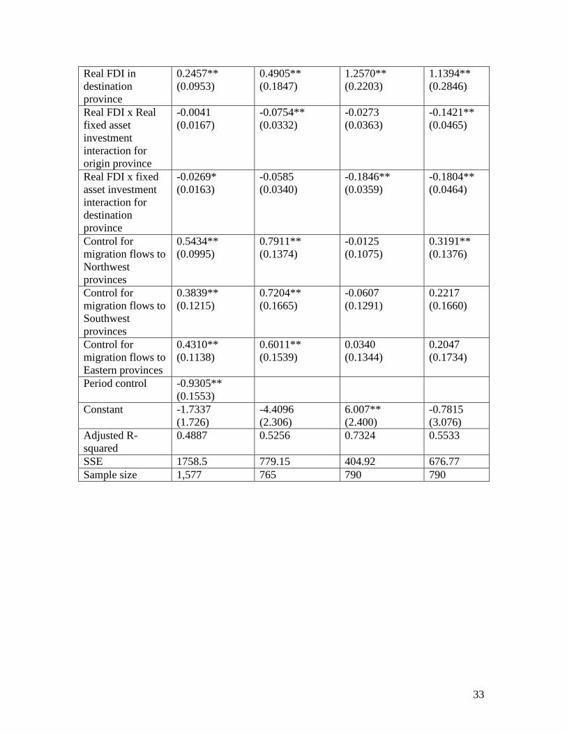
We obtain very mixed results for the estimated effects of fixed asset investment on

migration patterns. For the early period, there is as hypothesized an inverse relationship

between investment in the origin and out-migration, but the relationship is not

statistically significant. For the full sample and later period regressions, however, the

relationship is positive and significant, which disconfirms our hypothesis. In contrast, for

the later period a 1% increase in investment in the destination is estimated to increase in-

migration by just under 0.3%, confirming our hypothesis, but for the other regressions the

relationship between destination investment and in-migration is apparently negative. One

possible explanation for the positive relationship between origin investment and out-

migration is that more investment spending, by creating greater overall prosperity, could

help make out-migration more affordable than before.

While the coefficient estimates for real FDI in the origin province do not confirm our

hypothesis, the estimates for FDI in the destination are consistently supportive and

26

robust. For example, for the full sample regression, a 1% increase in destination FDI

induces a 0.25% increase in the in-migration rate, all other things equal. Note that the

responsiveness of in-migration to FDI is considerably greater during the 1990s, which

may reflect the effects of lower barriers to migration during that period. For example,

during the later period we estimate that when real FDI rises by 1%, in-migration rises by

over 1.25%.

We find strong evidence that the marginal effect of provincial fixed asset investment

(FDI) on migration rates is negatively influenced by the level of FDI (provincial fixed

asset investment). For example, for the full sample, when one type of investment in the

destination province rises by 1%, the marginal effect on migration of the other type of

investment will fall by approximately 0.03%. We obtain the same sort of result, although

stronger, for the later period. Furthermore, we find some evidence of a negative

interaction effect between both types of investment for the origin. We take these results

to suggest that foreign-financed and internally-financed investment projects in a province

may compete for imported labor, hence when imported labor supply to one type of

investment project rises, imported supply to the other will be less responsive.

For the full sample and early period regressions, ceteris paribus, migration rates to the

two Western sub-regions were higher than they were to the Central provinces, with

migration rates to the Southwest provinces being even higher. These results, taken

together, indicate that ceteris paribus Westward migration was higher over both periods,

but not during the 1990s. Migration rates to the Eastern provinces were also generally

higher than to the Central provinces, but only during the early period. However, all other

27

things equal, interprovincial migration rates nationwide were actually about 0.6% lower

during the 1990s.

V. CONCLUDING REMARKS

We have established in this study that, in addition to spatial differences in labor

market conditions, climate, and human capital endowments, there are other important

determinants of province-to-province migration flows in China. The most important of

these are migrant networks; migration during 1995-2000 appears to have been strongly

influenced by migration flows during the previous ten years. We found that when we

controlled for network effects in our regressions, the marginal effect of distance on

migration flows fell appreciably, thus the very strong effects of distance on migration

found in Lin, Wang and Zhao (2004) were likely to be upwardly biased due to the

omission of a migrant network control. Thus, in any study of internal migration in China,

it is crucial to control for past migration.

We find strong evidence that destination FDI encourages in-migration and some

evidence that destination fixed asset investment encourages in-migration. Higher levels

of fixed asset investment in the origin were found to be associated with higher levels of

out-migration, a result that requires further investigation. Our mixed results for the

investment variables suggest that further investigation of the relationship between

provincial investment spending and migration is needed. The majority of our results for

the variables used in previous studies of interprovincial migrant flows generally replicate

the findings of previous researchers. However, our evidence does not seem to offer much

28

support for earlier findings that as China’s economic reforms deepened during the 1990s,

the structure of migration changed.

For internal migration researchers, China is and will continue to be a significant

natural experiment in deregulation of migration, coinciding with national economic

prosperity, market-oriented reforms, foreign direct investment and globalization. There is

great need for future research on this subject, as interregional labor mobility will be a

prime contributor to China’s success in completing its transition to a market economy.

VI. REFERENCES

Bao, Shuming, Jack W. Hou and Anqing Shi (2006), “Migration and Regional

Development in China,” in Shuming Bao, Shuanglin Lin and Changwen Zhao (editors),

Chinese Economy after WTO Accession, Aldershot, UK: Ashgate.

Greenwood, Michael J. (1997), “Internal Migration in Developed Economies,” in

Handbook of Population and Family Economics (Mark R. Rosenzweig and Oded Stark,

editors), Amsterdam: Elsevier B.V., pp. 647-720.

Liang, Zai (2001), “The Age of Migration in China,” Population and Development

Review, 27, September, pp. 499-524.

Liang, Zai, Yiu Por Chen and Yanmin Gu (2002), “Rural Industrialisation and Internal

Migration in China,” Urban Studies, 39, 12, pp. 2175-87.

Liang, Zai and Michael J. White (1996), “Internal Migration in China, 1950-88,”

Demography, 33, August, pp. 375-84.

__________________________ (1997), “Market Transition, Government Policies, and

Interprovincial Migration in China: 1983-1988,” Economic Development and Cultural

Change, 45, 2, pp. 321-39.

Lin, Justin, Gewei Wang and Yaohui Zhao (2004), “Regional Inequality and Labor

Transfers in China,” Economic Development and Cultural Change, 52, April, pp. 587-

603.

Poncet, Sandra (2006), “Provincial Migration Dynamics in China: Borders, Costs and

Economic Motivations,” Regional Science and Urban Economics, 36, pp. 385-98.

29

Zhao, Yaohui (2002), “Causes and Consequences of Return Migration: Recent Evidence

from China,” Journal of Comparative Economics, 30, pp. 376-94.

___________ (1999a), “Labor Migration and Earnings Differences: The Case of Rural

China,” Economic Development and Cultural Change, 47, 4, pp. 767-82.

___________ (1997), “Labor Migration and Returns to Rural Education in China,”

American Journal of Agricultural Economics, 79, November, pp. 1278-87.

___________ (1999b), “Leaving the Countryside: Rural-to-Urban Migration Decisions in

China,” American Economic Review, 89, 2, pp. 281-86.

___________ (2003), “The Role of Migrant Networks in Labor Migration: The Case of

China,” Contemporary Economic Policy, 21, October, pp. 500-11.

30

TABLE 1

Summary Statistics for Provinces in 1980s sub-sample

(765 observations)

Variable Mean Standard

Deviation

Maximum Minimum

Province-to-

province emigration

rate (out of total

emigration from the

origin province)

3.7747% 6.9823% 79.336%

0.018047%

Real Mean Annual

FDI Per Capita

(Between 1980 and

1984)

$US 1.77 $US 6.57 $US 35.02 $US 0.01

Real Mean Annual

Fixed Asset

Investment Per

Capita (Between

1980 and 1984)

205.65 Yuan 167.58 Yuan 686.75 Yuan 57.65 Yuan

Railway distance

between capital

cities of origin and

destination

provinces

1,630.76

Kilometers

1.87 Kilometers 6,313.21

Kilometers

137

Kilometers

Mean per capita

income

507.82 Yuan 184.91 Yuan 1,084.53

Yuan

340.53 Yuan

Mean years of

schooling

6.426 1.248 9.463 4.379

Unemployment rate 1.214% 0.767% 4.11% 0.28%

Manufacturing

share of GDP

42.63% 9.81% 66.79% 20.56%

Mean yearly

temperature

14.113 C 5.176 C 24.517 C 4.608 C

Minority population

share

12.28% 16.06% 59.43% 0.31%

31

TABLE 2

Summary Statistics for Provinces in 1990s sub-sample

Variable Mean Standard

Deviation

Maximum Minimum

Province-to-

province

emigration rate

(out of total

emigration from

the origin

province)

3.5886% 7.2295% 87.317%

0.01436%

Number of persons

in the

destination’s pre-

existing migrant

community

24,985 68,541 893,200 100

Real Mean Annual

FDI Per Capita

(Between 1980

and 1984)

$US 9.95 $US 14.07 $US 50.53 $US 0.38

Real Mean Annual

Fixed Asset

Investment Per

Capita (Between

1980 and 1984)

563.55 Yuan 424.91 Yuan 1890.3 Yuan 160.31 Yuan

Railway distance

between capital

cities of origin

and destination

provinces

1,630.76 Kilometers 1.87 Kilometers 6,313.21

Kilometers

137 Kilometers

Manufacturing

share of GDP

44.52% 6.60% 54.9% 20.68%

Mean per capita

income

1,062.61 Yuan 447.27 Yuan 2,451.51 Yuan 605.26 Yuan

Mean years of

schooling

7.976 1.038 10.558 5.974

Unemployment

rate

4.392% 2.445% 9.64% 1.36%

Mean yearly

temperature

14.113 C 5.176 C 24.517 C 4.608 C

Minority

population share

12.28% 16.06% 59.43% 0.31%

32

TABLE 3

OLS REGRESSION RESULTS Dependent Variable = Gross Interprovincial Migration Rate

(Standard Errors in Parentheses; ** denotes significant at 1%, * at 5%,)

REGRESSOR

FULL

SAMPLE

EARLY

PERIOD ONLY

LATER

PERIOD ONLY

LATER

PERIOD

ONLY

Migrant Network 0.4910**

(0.0217)

Distance -1.2105**

(0.0493)

-1.3699**

(0.0702)

-0.4260**

(0.0556)

-1.0926**

(0.0610)

Real income in

origin

0.3068

(0.2002)

1.0637**

(0.2819)

-1.6691**

(0.2264)

-1.0326**

(0.29)

Real income in

destination

1.7622**

(0.2167)

1.9247**

(0.3098)

0.8110**

(0.2197)

1.0792**

(0.2835)

Education level in

origin

-1.6544**

(0.2714)

-1.4879**

(0.3271)

-2.6371**

(0.3862)

-2.589**

(0.499)

Education level in

destination

1.3741**

(0.2995)

1.4893**

(0.3634)

2.2344**

(0.3987)

2.1925**

(0.5151)

Unemployment

rate in origin

-0.2720**

(0.0812)

-0.1957*

(0.1143)

0.1166

(0.1002)

-0.0471

(0.1292)

Unemployment

rate in destination

-0.4750**

(0.0883)

-0.8347**

(0.1201)

-0.4479**

(0.1123)

-0.4871**

(0.1450)

Manufacturing

share of GDP in

origin

-0.4507

(0.2317)

-0.9580**

(0.3324)

-0.4494

(0.2473)

0.6828**

(0.3192)

Manufacturing

share of GDP in

destination

-0.7845**

(0.2340)

-2.3037**

(0.3380)

1.4966**

(0.2433)

1.0641

(0.3133)

Minority share in

origin

0.0255

(0.0220)

0.0659**

(0.0318)

0.0164

(0.0226)

0.0182

(0.0292)

Minority share in

destination

-0.0512

(0.0269)

-0.0926**

(0.0395)

0.0341

(0.0265)

0.0473

(0.0342)

Temperature in

origin

-0.6114**

(0.1159)

-0.4869**

(0.1695)

-0.2151

(0.1325)

-0.2239

(0.1712)

Temperature in

destination

-0.0377

(0.1193)

-0.7834**

(0.1867)

0.6940**

(0.1354)

0.6915**

(0.1750)

Real fixed asset

investment in

origin

0.3415**

(0.0843)

-0.0984

(0.1183)

1.8806**

(0.1389)

1.4036**

(0.1774)

Real fixed asset

investment in

destination

-0.4541**

(0.0908)

-0.5008**

(0.1192)

-0.3586**

(0.1537)

0.2938*

(0.1950)

Real FDI in origin 0.1436

(0.0966)

0.5186**

(0.1801)

0.2115

(0.2198)

0.9778**

(0.2806)

33

Real FDI in

destination

province

0.2457**

(0.0953)

0.4905**

(0.1847)

1.2570**

(0.2203)

1.1394**

(0.2846)

Real FDI x Real

fixed asset

investment

interaction for

origin province

-0.0041

(0.0167)

-0.0754**

(0.0332)

-0.0273

(0.0363)

-0.1421**

(0.0465)

Real FDI x fixed

asset investment

interaction for

destination

province

-0.0269*

(0.0163)

-0.0585

(0.0340)

-0.1846**

(0.0359)

-0.1804**

(0.0464)

Control for

migration flows to

Northwest

provinces

0.5434**

(0.0995)

0.7911**

(0.1374)

-0.0125

(0.1075)

0.3191**

(0.1376)

Control for

migration flows to

Southwest

provinces

0.3839**

(0.1215)

0.7204**

(0.1665)

-0.0607

(0.1291)

0.2217

(0.1660)

Control for

migration flows to

Eastern provinces

0.4310**

(0.1138)

0.6011**

(0.1539)

0.0340

(0.1344)

0.2047

(0.1734)

Period control -0.9305**

(0.1553)

Constant -1.7337

(1.726)

-4.4096

(2.306)

6.007**

(2.400)

-0.7815

(3.076)

Adjusted R-

squared

0.4887 0.5256 0.7324 0.5533

SSE 1758.5 779.15 404.92 676.77

Sample size 1,577 765 790 790