Interpreting CNNs via Decision Trees

Quanshi Zhang†, Yu Yang‡, Haotian Ma§, and Ying Nian Wu‡

†Shanghai Jiao Tong University, ‡University of California, Los Angeles,§South China University of Technology

Abstract

This paper1 aims to quantitatively explain the rationales

of each prediction that is made by a pre-trained convolu-

tional neural network (CNN). We propose to learn a deci-

sion tree, which clarifies the specific reason for each predic-

tion made by the CNN at the semantic level. I.e. the decision

tree decomposes feature representations in high conv-layers

of the CNN into elementary concepts of object parts. In this

way, the decision tree tells people which object parts ac-

tivate which filters for the prediction and how much each

object part contributes to the prediction score. Such seman-

tic and quantitative explanations for CNN predictions have

specific values beyond the traditional pixel-level analysis of

CNNs. More specifically, our method mines all potential de-

cision modes of the CNN, where each mode represents a typ-

ical case of how the CNN uses object parts for prediction.

The decision tree organizes all potential decision modes in

a coarse-to-fine manner to explain CNN predictions at dif-

ferent fine-grained levels. Experiments have demonstrated

the effectiveness of the proposed method.

1. Introduction

Convolutional neural networks (CNNs) [20, 18, 14] have

achieved superior performance in various tasks. However,

besides the discrimination power, model interpretability is

still a significant challenge for neural networks. Many s-

tudies have been proposed to visualize or analyze feature

representations hidden inside a CNN, in order to open the

black box of neural networks.

Motivation & objective: In the scope of network inter-

pretability, state-of-the-art algorithms are still far from the

ultimate goal of explaining why a CNN learns knowledge as

it is. Although some theories, such as the information bot-

tleneck [34], analyzed statistical characteristics of a neural

1Quanshi Zhang is the corresponding author with the John Hopcroft

Center and the MoE Key Lab of Artificial Intelligence, AI Institute, at the

Shanghai Jiao Tong University, China. Yu Yang and Ying Nian Wu are

with the University of California, Los Angeles, USA. Haotian Ma is with

the South China University of Technology, China.

...

Explanatory

tree

y=0.87

(b) grad-CAM(a) Input (c) Visualization of filters

(d)

Our

exp

lana

tions

Conv5-2 Conv3-3

Tail

Feature maps of a nape filter

Distribution of contributions of different filters

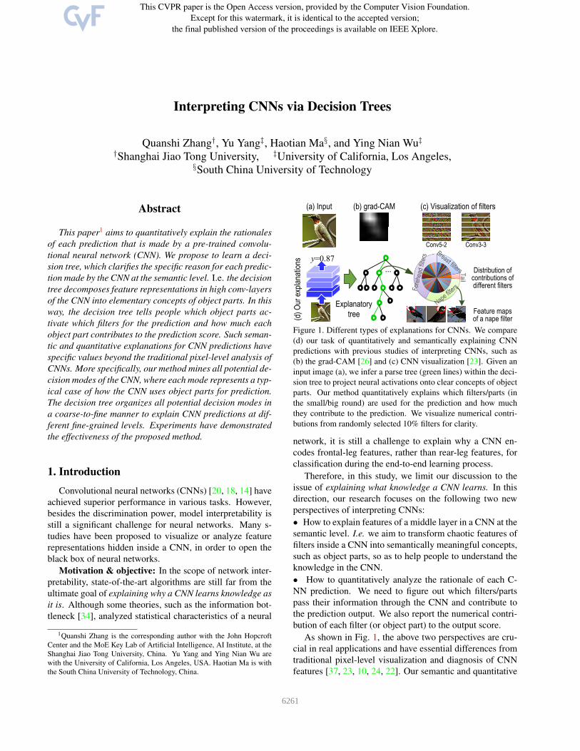
Figure 1. Different types of explanations for CNNs. We compare

(d) our task of quantitatively and semantically explaining CNN

predictions with previous studies of interpreting CNNs, such as

(b) the grad-CAM [26] and (c) CNN visualization [23]. Given an

input image (a), we infer a parse tree (green lines) within the deci-

sion tree to project neural activations onto clear concepts of object

parts. Our method quantitatively explains which filters/parts (in

the small/big round) are used for the prediction and how much

they contribute to the prediction. We visualize numerical contri-

butions from randomly selected 10% filters for clarity.

network, it is still a challenge to explain why a CNN en-

codes frontal-leg features, rather than rear-leg features, for

classification during the end-to-end learning process.

Therefore, in this study, we limit our discussion to the

issue of explaining what knowledge a CNN learns. In this

direction, our research focuses on the following two new

perspectives of interpreting CNNs:

• How to explain features of a middle layer in a CNN at the

semantic level. I.e. we aim to transform chaotic features of

filters inside a CNN into semantically meaningful concepts,

such as object parts, so as to help people to understand the

knowledge in the CNN.

• How to quantitatively analyze the rationale of each C-

NN prediction. We need to figure out which filters/parts

pass their information through the CNN and contribute to

the prediction output. We also report the numerical contri-

bution of each filter (or object part) to the output score.

As shown in Fig. 1, the above two perspectives are cru-

cial in real applications and have essential differences from

traditional pixel-level visualization and diagnosis of CNN

features [37, 23, 10, 24, 22]. Our semantic and quantitative

16261

... Most generic rationales

(our target)

Most specific rationales

Mode of a species with a specific pose

Mode of standing birds of various specieses

Dis

enta

ngle

d fil

ters

in th

e to

p co

nv-la

yer

y=0.9

...

FC

la

yers

A head filter

A feet filter

A torso filter

contribute 2.32%

contribute 0.72%

contribute 1.21%

A decision m

ode

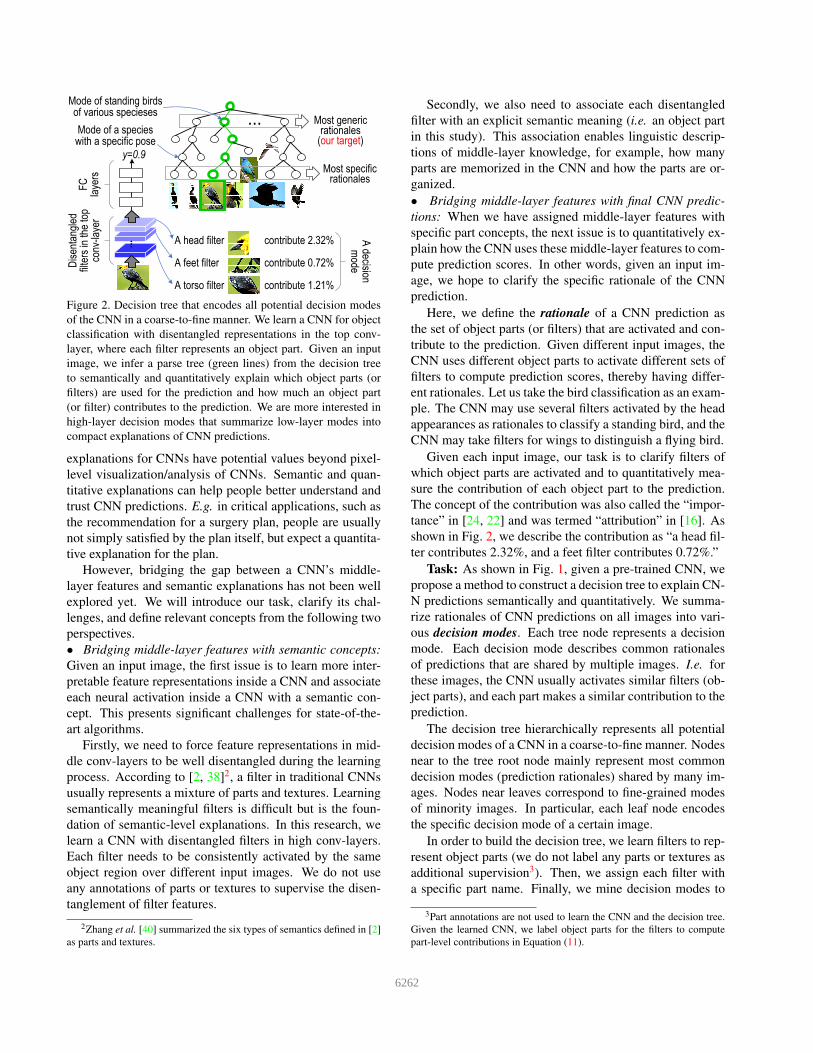
Figure 2. Decision tree that encodes all potential decision modes

of the CNN in a coarse-to-fine manner. We learn a CNN for object

classification with disentangled representations in the top conv-

layer, where each filter represents an object part. Given an input

image, we infer a parse tree (green lines) from the decision tree

to semantically and quantitatively explain which object parts (or

filters) are used for the prediction and how much an object part

(or filter) contributes to the prediction. We are more interested in

high-layer decision modes that summarize low-layer modes into

compact explanations of CNN predictions.

explanations for CNNs have potential values beyond pixel-

level visualization/analysis of CNNs. Semantic and quan-

titative explanations can help people better understand and

trust CNN predictions. E.g. in critical applications, such as

the recommendation for a surgery plan, people are usually

not simply satisfied by the plan itself, but expect a quantita-

tive explanation for the plan.

However, bridging the gap between a CNN’s middle-

layer features and semantic explanations has not been well

explored yet. We will introduce our task, clarify its chal-

lenges, and define relevant concepts from the following two

perspectives.

• Bridging middle-layer features with semantic concepts:

Given an input image, the first issue is to learn more inter-

pretable feature representations inside a CNN and associate

each neural activation inside a CNN with a semantic con-

cept. This presents significant challenges for state-of-the-

art algorithms.

Firstly, we need to force feature representations in mid-

dle conv-layers to be well disentangled during the learning

process. According to [2, 38]2, a filter in traditional CNNs

usually represents a mixture of parts and textures. Learning

semantically meaningful filters is difficult but is the foun-

dation of semantic-level explanations. In this research, we

learn a CNN with disentangled filters in high conv-layers.

Each filter needs to be consistently activated by the same

object region over different input images. We do not use

any annotations of parts or textures to supervise the disen-

tanglement of filter features.

2Zhang et al. [40] summarized the six types of semantics defined in [2]

as parts and textures.

Secondly, we also need to associate each disentangled

filter with an explicit semantic meaning (i.e. an object part

in this study). This association enables linguistic descrip-

tions of middle-layer knowledge, for example, how many

parts are memorized in the CNN and how the parts are or-

ganized.

• Bridging middle-layer features with final CNN predic-

tions: When we have assigned middle-layer features with

specific part concepts, the next issue is to quantitatively ex-

plain how the CNN uses these middle-layer features to com-

pute prediction scores. In other words, given an input im-

age, we hope to clarify the specific rationale of the CNN

prediction.

Here, we define the rationale of a CNN prediction as

the set of object parts (or filters) that are activated and con-

tribute to the prediction. Given different input images, the

CNN uses different object parts to activate different sets of

filters to compute prediction scores, thereby having differ-

ent rationales. Let us take the bird classification as an exam-

ple. The CNN may use several filters activated by the head

appearances as rationales to classify a standing bird, and the

CNN may take filters for wings to distinguish a flying bird.

Given each input image, our task is to clarify filters of

which object parts are activated and to quantitatively mea-

sure the contribution of each object part to the prediction.

The concept of the contribution was also called the “impor-

tance” in [24, 22] and was termed “attribution” in [16]. As

shown in Fig. 2, we describe the contribution as “a head fil-

ter contributes 2.32%, and a feet filter contributes 0.72%.”

Task: As shown in Fig. 1, given a pre-trained CNN, we

propose a method to construct a decision tree to explain CN-

N predictions semantically and quantitatively. We summa-

rize rationales of CNN predictions on all images into vari-

ous decision modes. Each tree node represents a decision

mode. Each decision mode describes common rationales

of predictions that are shared by multiple images. I.e. for

these images, the CNN usually activates similar filters (ob-

ject parts), and each part makes a similar contribution to the

prediction.

The decision tree hierarchically represents all potential

decision modes of a CNN in a coarse-to-fine manner. Nodes

near to the tree root node mainly represent most common

decision modes (prediction rationales) shared by many im-

ages. Nodes near leaves correspond to fine-grained modes

of minority images. In particular, each leaf node encodes

the specific decision mode of a certain image.

In order to build the decision tree, we learn filters to rep-

resent object parts (we do not label any parts or textures as

additional supervision3). Then, we assign each filter with

a specific part name. Finally, we mine decision modes to

3Part annotations are not used to learn the CNN and the decision tree.

Given the learned CNN, we label object parts for the filters to compute

part-level contributions in Equation (11).

6262

explain how the CNN use parts/filters for prediction, and

construct a decision tree.

Inference: When the CNN makes a prediction for an

input image, the decision tree determines a parse tree (see

green lines in Fig. 2) to encode a series of explanations.

Each node (decision mode) in the parse tree quantitatively

explains the prediction at a different abstraction level, i.e.

clarifying how much each object part/filter contributes to

the prediction score.

Compared to fine-grained modes in leave nodes, we are

more interested in generic decision modes in high-level

nodes. Generic decision modes usually select significan-

t object parts (filters) as the rationale of CNN predictions

and ignore insignificant ones. Thus, generic decision modes

reflect compact rationales for CNN predictions.

Contributions: In this paper, we aim to use semantic vi-

sual concepts to explain CNN predictions quantitatively and

semantically. We propose to learn the decision tree without

strong supervision for explanations. Our method is a gener-

ic approach and has been successfully applied to various

benchmark CNNs. Experiments have demonstrated the ef-

fectiveness of our method.

2. Related work

In this section, we limit our discussion to the literature

of opening the black box of CNN representations. [2, 21, 9,

4] discussed the definition of interpretability from different

perspectives concerning different tasks. Zhang et al. [43]

made a survey for the interpretability of deep visual models.

CNN visualization: Visualization of filters in a CNN is

the most direct way of exploring the pattern hidden inside a

neural unit. Gradient-based visualization [37, 23] estimates

the input image that maximizes the activation score of a

neural unit. Up-convolutional nets [10] invert feature maps

of conv-layers into images. Unlike gradient-based methods,

up-convolutional nets cannot mathematically ensure that the

visualization result reflects actual neural representations.

Zhou et al. [44] proposed a method to accurately com-

pute the image-resolution receptive field of neural activa-

tions in a feature map. The estimated receptive field of a

neural activation is smaller than the theoretical receptive

field based on the filter size. The accurate estimation of the

receptive field is crucial to understand a filter’s representa-

tions. Bau et al. [2] further defined six types of semantics

for CNNs, i.e. objects, parts, scenes, textures, materials,

and colors. Zhang et al. [38] summarized the six types of

semantics into “parts” and “textures.” Nevertheless, each

filter in a CNN represents a mixture of semantics. [45] ex-

plained semantic reasons for visual recognition.

Network diagnosis: Beyond visualization, some meth-

ods diagnose a pre-trained CNN to obtain insight under-

standing of CNN representations.

Fong and Vedaldi [11] analyzed how multiple filters

jointly represented a specific semantic concept. Yosinski

et al. [36] evaluated the transferability of filters in interme-

diate conv-layers. Aubry et al. [1] computed feature dis-

tributions of different categories in the CNN feature space.

Selvaraju et al. [26] and Fong et al. [12] propagated gradi-

ents of feature maps w.r.t. the CNN loss back to the image,

in order to estimate image regions that directly contribute

the network output. The LIME [24] and SHAP [22] ex-

tracted image regions that were used by a CNN to predict

a label. Zhang et al. [41] used an explainer network to in-

terpret object-part representations in intermediate layers of

CNNs.

Network-attack methods [17, 30] diagnosed network

representations by computing adversarial samples for a C-

NN. In particular, influence functions [17] were proposed

to compute adversarial samples, provide plausible ways to

create training samples to attack the learning of CNNs, fix

the training set, and further debug representations of a CN-

N. Lakkaraju et al. [19] discovered knowledge blind spot-

s (unknown patterns) of a pre-trained CNN in a weakly-

supervised manner. The study of [39] examined represen-

tations of conv-layers and automatically discover potential,

biased representations of a CNN due to the dataset bias.

CNN semanticization: Compared to the diagnosis of

CNN representations, some studies aim to learn more mean-

ingful CNN representations. Some studies extracted neural

units with clear semantics from CNNs for different applica-

tions. Given feature maps of conv-layers, Zhou et al. [44]

extracted scene semantics. Simon et al. mined objects from

feature maps of conv-layers [27], and learned object part-

s [28]. The capsule net [25] used a dynamic routing mech-

anism to parse the entire object into a parsing tree of cap-

sules. Each output dimension of a capsule in the network

may encode a specific meaning. Zhang et al. [40] proposed

to learn CNNs with disentangled intermediate-layer repre-

sentations. The infoGAN [6] and β-VAE [15] learned in-

terpretable input codes for generative models. Zhang et

al. [42] learned functionally interpretable, modular struc-

tures for neural networks via network transplanting.

Decision trees for neural networks: Distilling knowl-

edge from neural networks into tree structures is an emerg-

ing direction [13, 31, 5], but the trees did not explain the

network knowledge at a human-interpretable semantic lev-

el. Wu et al. [35] learned a decision tree via knowledge

distillation to represent the output feature space of an RN-

N, in order to regularize the RNN for better representation-

s. Vaughan et al. [32] distilled knowledge into an additive

model for explanation.

Despite the use of tree structures, there are two main d-

ifferences between the above two studies and our research.

Firstly, we focus on using a tree to explain each prediction

made by a pre-trained CNN semantically. In contrast, deci-

sion trees in the above studies are mainly learned for clas-

6263

Filter 1

Filter 2

Filter 3

Ordinary filters Disentangled filters

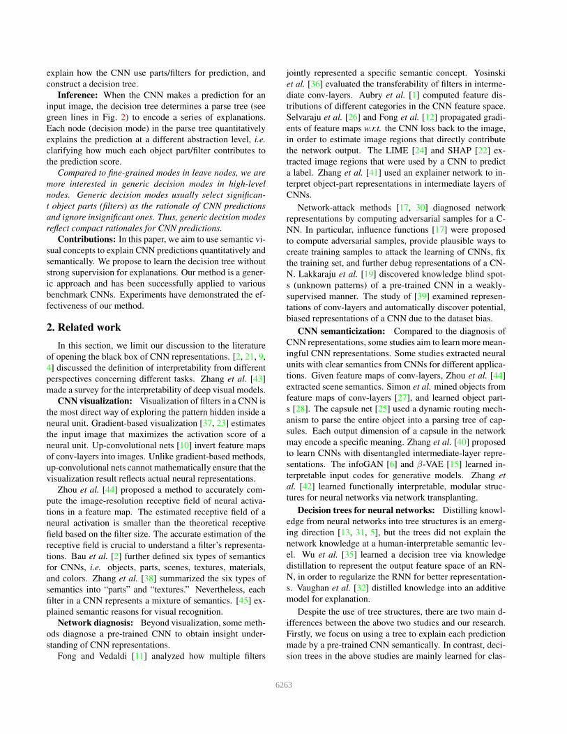
Figure 3. Comparisons between ordinary CNN feature maps and

disentangled feature maps that are used in this study. We visualize

image regions corresponding to each feature map based on [44].

sification and cannot provide semantic-level explanation-

s. Secondly, we summarize decision modes from gradients

w.r.t. neural activations of object parts as rationales to ex-

plain CNN prediction. Compared to the above “distillation-

based” methods, our “gradient-based” decision tree reflects

CNN predictions more directly and strictly.

3. Image-specific rationale of a CNN prediction

In this section, we design a method to simplify the com-

plex feature processing inside a CNN into a linear form

(i.e. Equation (3)), as the specific rationale of the predic-

tion w.r.t. the input image. This linear equation clarifies (i)

which object parts activate which filters in the CNN and (ii)

how much these parts/filters contribute to the final predic-

tion score.

In order to obtain semantic-level rationale of a CNN pre-

diction, we need (i) first to ensure that the CNN’s middle-

layer features are semantically meaningful, and (ii) then to

extract explicit contributions of middle-layer features to the

prediction score.

In this study, we learn the CNN for object classification.

Theoretically, we can interpret CNNs oriented to different

tasks. Nevertheless, in this paper, we limit our attention to

CNNs for classification, in order to simplify the story.

3.1. Learning disentangled filters

The basic idea is to revise a benchmark CNN, in order

to make each filter in the top conv-layer represent a specific

object part. We expect the filter to be automatically con-

verged to the representation of a part, instead of using addi-

tional part annotations to supervise the learning process.

We apply the filter loss [40] to each filter in the top conv-

layer to push the filter towards the representation of an ob-

ject part. As shown in Fig. 3, the filter is learned to be acti-

vated by the same object part given different input images.

Theoretically, our method also supports other techniques of

mining interpretable features in middle layers [38, 27]. N-

evertheless, the filter loss usually ensures more meaningful

features than the other approaches.Filter loss: Let xf ∈ R

L×L denote the feature map ofa filter f . Without part annotations, the filter loss forces xf

to be exclusively activated by a specific part of a category.We can summarize the filter loss as the minus mutual infor-

mation between the distribution of feature maps and that ofpart locations.

Lossf =∑

xf∈Xf

Lossf (xf ) = −MI(Xf ;P)

=−∑

µ∈Pp(µ)

∑

xf∈Xf

p(xf |µ) logp(xf |µ)

p(xf )

(1)

where MI(·) indicates the mutual information. Xf denotes

a set of feature maps of f extracted from different input

images. P = µ|µ = [h,w], 1 ≤ h,w ≤ L ∪ ∅ is referred

to as a set of all part-location candidates. Each location µ =[h,w] corresponds to an activation unit in xf . Besides, ∅ ∈P denotes the case that the target part does not appear in the

input image. In this case, all units in xf are expected to keep

inactivated. The joint probability p(xf , µ) to describe the

compatibility between xf and µ (please see [40] for details).

The filter loss ensures that given an input image, xf

should match only one of all L2+1 location candidates. It is

assumed that repetitive shapes on various regions are more

likely to describe low-level textures than high-level parts. If

the part appears, xf should have a single activation peak at

the part location; otherwise, xf should keep inactivated.

3.2. Quantitative rationales of CNN predictions

As analyzed in [2], filters in high conv-layers are more

prone to represent object parts, while those in low conv-

layers usually describe textures. Therefore, we choose fil-

ters in the top conv-layer to represent object parts. Con-

sequently, we quantitatively analyze how fully-connected

(FC) layers use object-part features from the top conv-layer

to make final predictions, as the rationale.

Given an input image I , let x ∈ RL×L×D denote the

feature map of the top conv-layer after a ReLU operation,

where L denotes the scale of the feature map, and D is the

filter number. Let y denote the scalar classification score of

a certain category before the softmax operation (when the

CNN is learned for multiple categories, we may learn a spe-

cific decision tree to explain the output of each category).

Our task is to use x to represent the rationale of y.As discussed in [22, 24], we can use a piecewise linear

representation to represent the function of cascaded FC lay-ers and ReLU layers, as follows.

y = ffc-n(frelu(· · · ffc-1(x))) =∑

h,w,d

g(h,w,d) · x(h,w,d) + b (2)

where x(h,w,d) ∈ R denotes the element at the location

(h,w) of the d-th channel; g(h,w,d) is a weight that describes

the importance of x(h,w,d) for the prediction on I . Theoreti-

cally, we can compute g= ∂y

∂xand b=y − g ⊗ x.

We use weights g to denote the specific rationale of the

prediction for the input image. g(h,w,d)x(h,w,d) measures

x(h,w,d)’s quantitative contribution to the prediction.

Different input images correspond to different weights

g, i.e. different rationales of their CNN predictions. It is

6264

Filter 1:Filter 2:

…Filter D-1:

Filter D:

head patterntorso pattern

feet patterntail pattern

...u

v v’

u

’

...u

v v’u’

...v v’

0Q P 1P 2P

...

Figure 4. Learning a decision tree. Green lines in P3 indicate a

parse tree to explain the rationale of the prediction on an image.

because different images have various signal passing routes

through ReLU layers. Given an input images I , the CNN

uses certain weight values that are specific to I .

Because each interpretable filter only has a single activa-

tion peak [40], we can further compute vectors x,g ∈ RD

as an approximation to the tensors x, ∂y

∂x∈ R

L×L×D to sim-

plify the computation. We get x(d) = 1sd

∑

h,w x(h,w,d) and

g(d) = sdL2

∑

h,w∂y

∂x(h,w,d) , where x(d) denotes the d-th ele-

ment of x. sd = EIEh,w x(h,w,d) is used to normalize the

activation magnitude of the d-th filter.In this way, we can consider x and g to represent predic-

tion rationales4, i.e. using which filters/parts for prediction.

y ≈ gTx+ b (3)

Different dimensions of the vector x measure the scalar

signal strength of different object parts, since a filter poten-

tially represents a certain object part. g corresponds to the

selection of object parts for the CNN prediction.

4. Learning a decision tree

We learn a decision tree to interpret the classification of

each category. In the following two subsections, we first

define basic concepts in a decision tree and then introduce

the learning algorithm.

4.1. Decision tree

Let us focus on the decision tree for a certain category.

We consider images of this category as positive images and

consider other images as negative images. Ω+ denotes im-

age indexes of the target category, i.e. positive images, and

Ω = Ω+ ∪Ω− represents all training images. For an image

Ii (i ∈ Ω), yi denotes the classification score of the target

category before the softmax layer.

As shown in Fig. 2, each node v in the decision tree en-

codes a decision mode that is hidden inside FC layers of the

CNN. A decision mode represents a common rationale of

the prediction shared by a group of positive training images

Ωv ⊂ Ω+. The decision tree organizes the hierarchy of deci-

sion modes in a coarse-to-fine manner from the root node to

4Without loss of generality, we normalize g to a unit vector for more

convincing results: y←y/‖g‖, g←g/‖g‖, and b←b/‖g‖.

Algorithm 1 Learning a decision tree for a category

Input: 1. A CNN with disentangled filters, 2. training

images Ω = Ω+ ∪Ω−.

Output: A decision tree.

Initialize a tree Q = P0 and set t = 0for each image Ii, i ∈ Ω+ do

Initialize a child of the root of the initial tree Q by

setting g=gi based on Equation (3) and α=1.

end for

for t = t+ 1 until ∆ logE ≤ 0 do

1. Choose (v, v′) in the second tree layer of Pt−1 that

maximize ∆ logE based on Equation (8)

2. Merge (v, v′) to generate a new node u based on

Equations (5) and (6), and obtain the tree Pt.

end for

Assign filters with semantic object parts to obtain A.

leaf nodes. Children nodes v′ ∈ Child(v) divides the paren-

t v’s decision mode into fine-grained modes. Fine-grained

modes are shared by sub-groups of images.Just like the rationale defined in Equation (3), the deci-

sion mode in node v is parameterized with w and b, andthe mode explains predictions on a certain set of images Ωv.For each image Ii, i ∈ Ωv, the decision mode is given as

hv(xi) = wTxi + b, w = α g (4)

maxg

∑

i∈Ωvcosine(gi,g), s.t. gTg = 1 (5)

minα,b1

‖Ωv‖

∑

i∈Ωv(wTxi + b− yi)

2 + λ‖α‖1 (6)

where w is referred to as the rationale of the decision mode.

g is a unit vector (‖g‖2=1) that reflects common rationales

that are shared by all images in Ωv. α ∈ 0, 1D is given

as a binary selection of filters in the decision mode. de-

note element-wise multiplications. We compute sparse α to

obtain sparse explanations for the decision mode5.

In particular, when v is a leaf node, the decision mode is

formulated as the rationale of a specific image Ii. I.e. α =

[1, 1, . . . , 1]T and w = α gi = gi, where gi is computed in

Equation (3).

4.2. Learning decision trees

Just like hierarchical clustering, the basic idea of learn-

ing a decision tree is to summarize common generic deci-

sion modes from specific decision modes of different im-

ages. Algorithm 1 shows the pseudo-code of the learning

process. At the beginning, we initialize the decision mode

gi of each positive image Ii as a leaf node by setting g=gi

and α = 1. Thus, we build an initial tree Q as shown in

Fig. 4, in which the root node takes decision modes of all

positive images as children. Then, in each step, we select

and merge two nodes v, v′ ∈ V in the second tree layer (i.e.

children of the root node) to obtain a new node u, where Vdenotes the children set of the root. u becomes a new child

6265

of the root node, and v and v′ are re-assigned as u’s chil-

dren. The image set of u is defined as Ωu = Ωv ∪ Ωv′ and

we learn α, b,g for u based on Equations (5) and (6).In this way, we gradually revise the initial tree P0 = Q

towards the final tree after T merging operations as

Q = P0 → P1 → P2 → · · · → PT = P (7)

We formulate the objective for learning as follows.

maxP

E, E =

∏

i∈Ω+ P (xi)∏

i∈Ω+ Q(xi)︸ ︷︷ ︸

Discrimination power

· e−β‖V ‖

︸ ︷︷ ︸

Sparsity ofdecision modes

(8)

where P (xi) denotes the likelihood of xi being positivethat is estimated by the tree P . β is a scaling parameter5.This objective penalizes the decrease of the discriminativepower and forces the system to summarize a few genericdecision modes for explanation. We compute the likelihoodof xi being positive as

P (xi) = eγh(xi)/∑

j∈Ωeγh(xj) (9)

where h(xi)=hv(xi) denotes the prediction on xi based on

best child v ∈ V in the second tree layer. γ is a constant

scaling parameter5.

In the t-th step, we merge two nodes v, v′ ∈ V in the

second tree layer of Pt−1 to get a new node u, thereby

obtaining a new tree Pt. We can easily compute ∆ logE

w.r.t. each pair of (v, v′) based on Equation (8). Thus, we

learn the decision tree via a greedy strategy. In each step,

we select and merge the nodes v, v′ ∈ V that maximize∆ logE

‖Ωv‖+‖Ωv′‖. We normalize ∆ logE for reasonable cluster-

ing performance. Because each node merger operation only

affects h(xi) values of a few examples in Ωv ∪ Ωv′ , we can

quickly estimate ∆ logE for each pair of nodes (v, v′).

4.3. Interpreting CNNs

Given a testing image Ii, the CNN makes a predictionyi. The decision tree estimates quantitative decision modesof the prediction at different fine-grained levels. During theinference procedure, we can infer a parse tree, which startsfrom the root node, in a top-down manner. Green lines inFig. 4 show a parse tree. When we select the decision modein the node u as the rationale, we can further select its childv that maximizes the compatibility with the most specificrationale gi as a more fine-grained mode:

v = argmaxv∈Child(u)cosine(gi,wv) (10)

where we add the subscript v to differentiate the parameter

of v from parameters of other nodes.A node v in the parse tree provides the rationale of the

prediction on image Ii at a certain fine-grained level. Wecompute the vector ρi and ˆi to evaluate the contribution ofdifferent filters and that of different object parts.

ρi = wv xi, ˆi = Aρi (11)

5Please see the experiment section for settings of β, γ, and λ.

where the d-th element of ρi ∈ RD, ρ

(d)i , denotes the contri-

bution to the CNN prediction that is made by the d-th filter.

If ρ(d)i > 0, then the d-th object part makes a positive con-

tribution. If ρ(d)i < 0, then the d-th filter makes a negative

contribution. Based on visualization results in Figs. 3 and

6, we label a matrix A ∈ 0, 1M×D to assign each filter in

the top conv-layer with a specific object part, where M is

the part number. Each filter is assigned to a certain part, and

the annotation cost is O(M). Similarly, the m-th element of

ˆi ∈ RM , ˆ

(m)i measures the contribution of the m-th part.

5. Experiments

Implementation details: We learned four types of dis-

entangled CNNs based on structures of four benchmark C-

NNs, including the AlexNet [18], the VGG-M network [29],

the VGG-S network [29], the VGG-16 network [29]. Note

that as discussed in [40], the filter loss in the explainer is

not compatible with skip connections in residual network-

s [14]. We followed the technique of [40] to modify an or-

dinary CNN to a disentangled CNN, which changed the top

conv-layer of the CNN to a disentangled conv-layer and fur-

ther added a disentangled conv-layer on the top conv-layer.

We used feature maps of the new top conv-layer as the in-

put of our decision tree. We loaded parameters of all old

conv-layers directly from the CNN that was pre-trained us-

ing images in the ImageNet ILSVRC 2012 dataset [8] with a

loss for 1000-category classification. We initialized param-

eters of the new top conv-layer and all FC layers. Inspired

by previous studies of [40], we can weaken the problem of

multi-category classification as a number of single-category

classification to simplify the evaluation of interpretability.

Thus, we fine-tuned the CNN for binary classification of a

single category from random images with the log logistic

loss using three benchmark datasets. We simply set param-

eters as β = 1, γ = 1/Ei∈Ω+ [yi], and λ= 10−6√

‖Ωv‖ in all

experiments for fair comparisons.

Datasets: Because the quantitative explanation of CNN

predictions requires us to assign each filter in the top conv-

layer with a specific object part, we used three benchmark

datasets with ground-truth art annotations to evaluate our

method. The selected datasets include the PASCAL-Part

Dataset [7], the CUB200-2011 dataset [33], and the ILSVR-

C 2013 DET Animal-Part dataset [38]. Just like in most

part-localization studies [7, 38], we used animal categories,

which prevalently contain non-rigid shape deformation, for

evaluation. I.e. we selected six animal categories—bird,

cat, cow, dog, horse, and sheep—from the PASCAL Part

Dataset. The CUB200-2011 dataset contains 11.8K images

of 200 bird species. Like in [3, 28], we ignored species la-

bels and regarded all these images as a single bird category.

The ILSVRC 2013 DET Animal-Part dataset [38] consist-

s of 30 animal categories among all the 200 categories for

object detection in the ILSVRC 2013 DET dataset [8].

6266

1

2 3

1 2 31

2 3

12 3

1

2 3

1 2 31

2 3

1 2 3

1

2 3

1 2 31

2 3

1 2 3

1

2

3

1 2 31

2

3

1 2 31

2

3

1 2 31

2

3

1 2 3

Figure 5. Visualization of decision modes corresponding to nodes in the 2nd tree layer. We show typical images of each decision mode.

Input Activation distribution

Contribution distribution

Input Activation distribution

Contribution distribution

Filter for

cat torso

Filter for

cat head

Filter for

bird nape

Filter for

bird breast

Image receptive fields of a filter on different images

Figure 6. Object-part contributions for CNN prediction. Pie charts show contribution proportions of different parts, which are estimated

using nodes in the second tree layer. Heat maps indicate spatial distributions of neural activations in the top conv-layer (note that the

heat maps do not represent distributions of “contributions,” because neural activations are not weighted by gi). Right figures show image

receptive fields of different filters estimated by [44]. Based on these receptive filters, we assign the filters with different object parts to

compute the distribution of object-part contributions.

Analysis of object parts for prediction: We analyzed

the contribution of different object parts in the CNN pre-

diction, when we assigned each filter with a specific ob-

ject part. The vector ˆi in Equation (11) specifies the

contribution of different object parts in the prediction of

yi. For the m-th object part, we computed contrim =

| ˆ(m)i |/

∑M

m′=1 | ˆ(m′)i | as the ratio of the part’s contribution.

More specifically, for CNNs based on the ILSVRC 2013

DET Animal-Part dataset, we manually labeled the object

part for each filter in the top conv-layer. For CNNs based

on the Pascal VOC Part dataset [7], the study of [40] merged

tens of small parts into several major landmark parts for the

six animal categories. Given a CNN for a certain catego-

ry, we used [44] to estimate regions in different images that

corresponded to each filter’s neural activations, namely the

image receptive field of the filter (please see Figs. 6 and

3). For each filter, we selected a part from all major land-

mark parts, which was closest to the filter’s image receptive

field through all positive images. For the CNN based on the

CUB200-2011 dataset, we used ground-truth positions of

the breast, forehead, nape, tail of birds as major landmark

parts. Similarly, we assigned each filter in the top conv-

layer with the nearest landmark part.

Evaluation metrics: The evaluation has two aspects.

Firstly, we use two metrics to evaluate the accuracy of the

estimated rationale of a prediction. The first metric eval-

uates errors of object-part contributions to the CNN pre-

diction that were estimated using nodes in the second tree

layer. Given an input image I , ˆi in Equation (11) denotes

the quantitative contribution of the i-th part. Accordingly,

ˆ∗i =y − yi is referred to as the ground-truth contribution of

the part, where y denotes the original CNN prediction on I;

yi is the output when we removed neural activations from

feature maps (filters) corresponding to the i-th part. In this

way, we used the deviation EI∈I[ˆi − ˆ∗i ]/EI∈I[y] to de-

note the error of the i-th part contributions. Another metric,

namely the fitness of contribution distributions, compares

the ground-truth contribution distribution over different fil-

ters in the top conv-layer with the estimated contribution of

these filters during the prediction process. When the deci-

sion tree uses node v to explain the prediction for Ii, the

vector ρi in Equation (11) denotes the estimated contribu-

tion distribution of different filters. ti=gi xi correspond-

s to the ground-truth contribution distribution. We report-

ed the interaction-of-the-union value between ρi and ti to

measure the fitness of the ground-truth and the estimated

filter contribution distributions. I.e. we computed the fit-

ness as Ei∈Ω+ [min(ρ

(d)i

,|t(d)i

|)

max(ρ(d)i

,|t(d)i

|)], where t

(d)i denotes the d-th

element of ti and ρ(d)i = maxρ

(d)i sign(t

(d)i ), 0. We used

non-negative values of ρ(d)i and |t

(d)i |, because vectors ρi

and ti may have negative elements.

Secondly, in addition to the accuracy of the rationale, we

also measured the information loss of using the decision tree

to represent a CNN, as a supplementary evaluation. A met-

ric is the classification accuracy. Because h(xi) denotes

the prediction of yi based on the best child in the second

tree layer, we regarded h(·) as the output of the tree and we

evaluated the discrimination power of h(·). We used val-

ues of h(xi) for classification and compared its classifica-

tion accuracy with the accuracy of the CNN. Another met-

ric, namely the prediction error, measures the error of the

6267

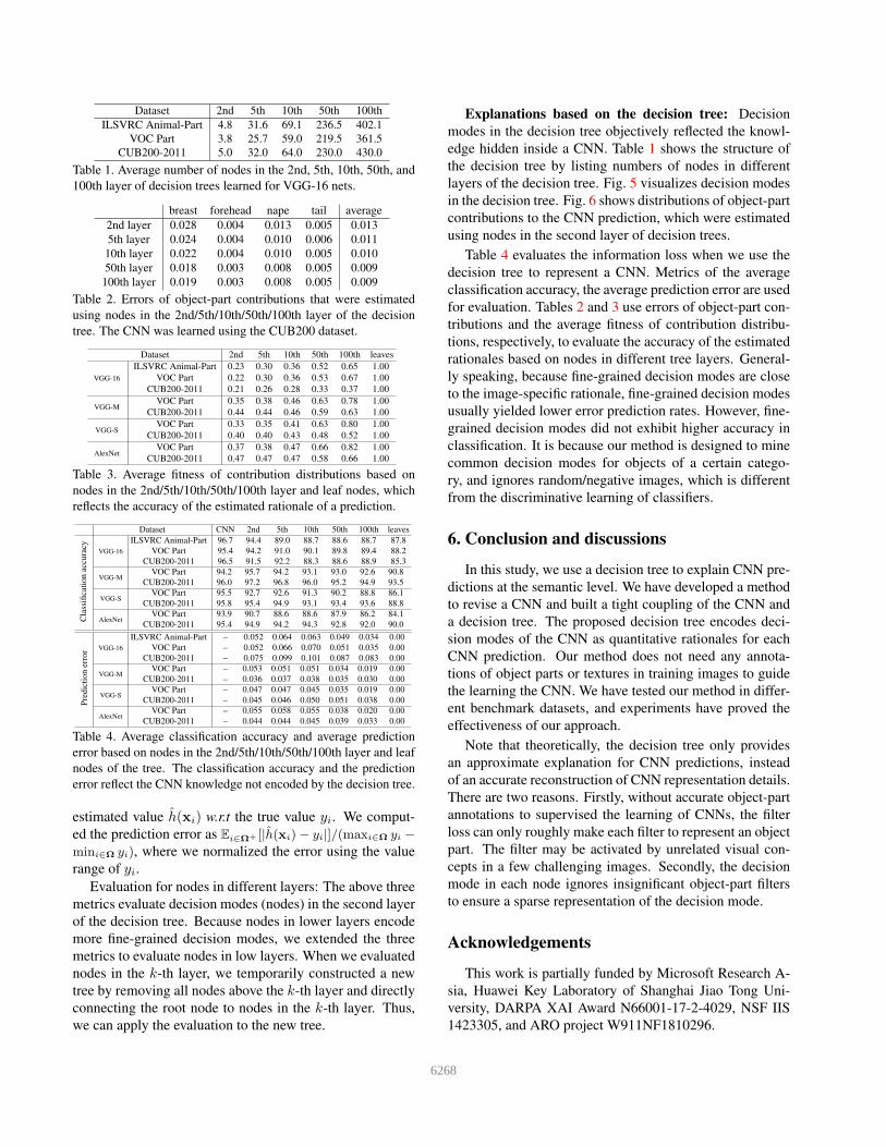
Dataset 2nd 5th 10th 50th 100th

ILSVRC Animal-Part 4.8 31.6 69.1 236.5 402.1

VOC Part 3.8 25.7 59.0 219.5 361.5

CUB200-2011 5.0 32.0 64.0 230.0 430.0

Table 1. Average number of nodes in the 2nd, 5th, 10th, 50th, and

100th layer of decision trees learned for VGG-16 nets.

breast forehead nape tail average

2nd layer 0.028 0.004 0.013 0.005 0.013

5th layer 0.024 0.004 0.010 0.006 0.011

10th layer 0.022 0.004 0.010 0.005 0.010

50th layer 0.018 0.003 0.008 0.005 0.009

100th layer 0.019 0.003 0.008 0.005 0.009

Table 2. Errors of object-part contributions that were estimated

using nodes in the 2nd/5th/10th/50th/100th layer of the decision

tree. The CNN was learned using the CUB200 dataset.

Dataset 2nd 5th 10th 50th 100th leaves

VGG-16

ILSVRC Animal-Part 0.23 0.30 0.36 0.52 0.65 1.00

VOC Part 0.22 0.30 0.36 0.53 0.67 1.00

CUB200-2011 0.21 0.26 0.28 0.33 0.37 1.00

VGG-MVOC Part 0.35 0.38 0.46 0.63 0.78 1.00

CUB200-2011 0.44 0.44 0.46 0.59 0.63 1.00

VGG-SVOC Part 0.33 0.35 0.41 0.63 0.80 1.00

CUB200-2011 0.40 0.40 0.43 0.48 0.52 1.00

AlexNetVOC Part 0.37 0.38 0.47 0.66 0.82 1.00

CUB200-2011 0.47 0.47 0.47 0.58 0.66 1.00

Table 3. Average fitness of contribution distributions based on

nodes in the 2nd/5th/10th/50th/100th layer and leaf nodes, which

reflects the accuracy of the estimated rationale of a prediction.

Dataset CNN 2nd 5th 10th 50th 100th leaves

Cla

ssifi

cati

on

accu

racy

VGG-16

ILSVRC Animal-Part 96.7 94.4 89.0 88.7 88.6 88.7 87.8

VOC Part 95.4 94.2 91.0 90.1 89.8 89.4 88.2

CUB200-2011 96.5 91.5 92.2 88.3 88.6 88.9 85.3

VGG-MVOC Part 94.2 95.7 94.2 93.1 93.0 92.6 90.8

CUB200-2011 96.0 97.2 96.8 96.0 95.2 94.9 93.5

VGG-SVOC Part 95.5 92.7 92.6 91.3 90.2 88.8 86.1

CUB200-2011 95.8 95.4 94.9 93.1 93.4 93.6 88.8

AlexNetVOC Part 93.9 90.7 88.6 88.6 87.9 86.2 84.1

CUB200-2011 95.4 94.9 94.2 94.3 92.8 92.0 90.0

Pre

dic

tion

erro

r VGG-16

ILSVRC Animal-Part – 0.052 0.064 0.063 0.049 0.034 0.00

VOC Part – 0.052 0.066 0.070 0.051 0.035 0.00

CUB200-2011 – 0.075 0.099 0.101 0.087 0.083 0.00

VGG-MVOC Part – 0.053 0.051 0.051 0.034 0.019 0.00

CUB200-2011 – 0.036 0.037 0.038 0.035 0.030 0.00

VGG-SVOC Part – 0.047 0.047 0.045 0.035 0.019 0.00

CUB200-2011 – 0.045 0.046 0.050 0.051 0.038 0.00

AlexNetVOC Part – 0.055 0.058 0.055 0.038 0.020 0.00

CUB200-2011 – 0.044 0.044 0.045 0.039 0.033 0.00

Table 4. Average classification accuracy and average prediction

error based on nodes in the 2nd/5th/10th/50th/100th layer and leaf

nodes of the tree. The classification accuracy and the prediction

error reflect the CNN knowledge not encoded by the decision tree.

estimated value h(xi) w.r.t the true value yi. We comput-

ed the prediction error as Ei∈Ω+ [|h(xi)− yi|]/(maxi∈Ω yi −

mini∈Ω yi), where we normalized the error using the value

range of yi.Evaluation for nodes in different layers: The above three

metrics evaluate decision modes (nodes) in the second layer

of the decision tree. Because nodes in lower layers encode

more fine-grained decision modes, we extended the three

metrics to evaluate nodes in low layers. When we evaluated

nodes in the k-th layer, we temporarily constructed a new

tree by removing all nodes above the k-th layer and directly

connecting the root node to nodes in the k-th layer. Thus,

we can apply the evaluation to the new tree.

Explanations based on the decision tree: Decision

modes in the decision tree objectively reflected the knowl-

edge hidden inside a CNN. Table 1 shows the structure of

the decision tree by listing numbers of nodes in different

layers of the decision tree. Fig. 5 visualizes decision modes

in the decision tree. Fig. 6 shows distributions of object-part

contributions to the CNN prediction, which were estimated

using nodes in the second layer of decision trees.

Table 4 evaluates the information loss when we use the

decision tree to represent a CNN. Metrics of the average

classification accuracy, the average prediction error are used

for evaluation. Tables 2 and 3 use errors of object-part con-

tributions and the average fitness of contribution distribu-

tions, respectively, to evaluate the accuracy of the estimated

rationales based on nodes in different tree layers. General-

ly speaking, because fine-grained decision modes are close

to the image-specific rationale, fine-grained decision modes

usually yielded lower error prediction rates. However, fine-

grained decision modes did not exhibit higher accuracy in

classification. It is because our method is designed to mine

common decision modes for objects of a certain catego-

ry, and ignores random/negative images, which is different

from the discriminative learning of classifiers.

6. Conclusion and discussions

In this study, we use a decision tree to explain CNN pre-

dictions at the semantic level. We have developed a method

to revise a CNN and built a tight coupling of the CNN and

a decision tree. The proposed decision tree encodes deci-

sion modes of the CNN as quantitative rationales for each

CNN prediction. Our method does not need any annota-

tions of object parts or textures in training images to guide

the learning the CNN. We have tested our method in differ-

ent benchmark datasets, and experiments have proved the

effectiveness of our approach.

Note that theoretically, the decision tree only provides

an approximate explanation for CNN predictions, instead

of an accurate reconstruction of CNN representation details.

There are two reasons. Firstly, without accurate object-part

annotations to supervised the learning of CNNs, the filter

loss can only roughly make each filter to represent an object

part. The filter may be activated by unrelated visual con-

cepts in a few challenging images. Secondly, the decision

mode in each node ignores insignificant object-part filters

to ensure a sparse representation of the decision mode.

Acknowledgements

This work is partially funded by Microsoft Research A-

sia, Huawei Key Laboratory of Shanghai Jiao Tong Uni-

versity, DARPA XAI Award N66001-17-2-4029, NSF IIS

1423305, and ARO project W911NF1810296.

6268

References

[1] M. Aubry and B. C. Russell. Understanding deep features

with computer-generated imagery. In ICCV, 2015. 3

[2] D. Bau, B. Zhou, A. Khosla, A. Oliva, and A. Torralba. Net-

work dissection: Quantifying interpretability of deep visual

representations. In CVPR, 2017. 2, 3, 4

[3] S. Branson, P. Perona, and S. Belongie. Strong supervision

from weak annotation: Interactive training of deformable

part models. In ICCV, 2011. 6

[4] A. Chandrasekaran, V. Prabhu, D. Yadav, P. Chattopadhyay,

and D. Parikh. Do explanations make vqa models more pre-

dictable to a human? In EMNLP, 2018. 3

[5] Z. Che, S. Purushotham, R. Khemani, and Y. Liu. Inter-

pretable deep models for icu outcome prediction. In Amer-

ican Medical Informatics Association (AMIA) Annual Sym-

posium, 2016. 3

[6] X. Chen, Y. Duan, R. Houthooft, J. Schulman, I. Sutskever,

and P. Abbeel. Infogan: Interpretable representation learning

by information maximizing generative adversarial nets. In

NIPS, 2016. 3

[7] X. Chen, R. Mottaghi, X. Liu, S. Fidler, R. Urtasun, and

A. Yuille. Detect what you can: Detecting and representing

objects using holistic models and body parts. In CVPR, 2014.

6, 7

[8] J. Deng, W. Dong, R. Socher, L.-J. Li, K. Li, and L. Fei-

Fei. Imagenet: A large-scale hierarchical image database. In

CVPR, 2009. 6

[9] F. Doshi-Velez and B. Kim. Towards a rigorous science of

interpretable machine learning. In arXiv:1702.08608, 2017.

3

[10] A. Dosovitskiy and T. Brox. Inverting visual representations

with convolutional networks. In CVPR, 2016. 1, 3

[11] R. Fong and A. Vedaldi. Net2vec: Quantifying and explain-

ing how concepts are encoded by filters in deep neural net-

works. In CVPR, 2018. 3

[12] R. C. Fong and A. Vedaldi. Interpretable explanation-

s of black boxes by meaningful perturbation. In arX-

iv:1704.03296v1, 2017. 3

[13] N. Frosst and G. Hinton. Distilling a neural network into a

soft decision tree. In arXiv:1711.09784, 2017. 3

[14] K. He, X. Zhang, S. Ren, and J. Sun. Deep residual learning

for image recognition. In CVPR, 2016. 1, 6

[15] I. Higgins, L. Matthey, A. Pal, C. Burgess, X. Glorot,

M. Botvinick, S. Mohamed, and A. Lerchner. β-vae: learn-

ing basic visual concepts with a constrained variational

framework. In ICLR, 2017. 3

[16] P.-J. Kindermans, K. T. Schutt, M. Alber, K.-R. Muller,

D. Erhan, B. Kim, and S. Dahne. Learning how to explain

neural networks: Patternnet and patternattribution. In ICLR,

2018. 2

[17] P. Koh and P. Liang. Understanding black-box predictions

via influence functions. In ICML, 2017. 3

[18] A. Krizhevsky, I. Sutskever, and G. E. Hinton. Imagenet

classification with deep convolutional neural networks. In

NIPS, 2012. 1, 6

[19] H. Lakkaraju, E. Kamar, R. Caruana, and E. Horvitz. Iden-

tifying unknown unknowns in the open world: Representa-

tions and policies for guided exploration. In AAAI, 2017. 3

[20] Y. LeCun, L. Bottou, Y. Bengio, and P. Haffner. Gradient-

based learning applied to document recognition. In Proceed-

ings of the IEEE, 1998. 1

[21] Z. C. Lipton. The mythos of model interpretability. In Com-

munications of the ACM, 61:36–43, 2018. 3

[22] S. M. Lundberg and S.-I. Lee. A unified approach to inter-

preting model predictions. In NIPS, 2017. 1, 2, 3, 4

[23] A. Mahendran and A. Vedaldi. Understanding deep image

representations by inverting them. In CVPR, 2015. 1, 3

[24] M. T. Ribeiro, S. Singh, and C. Guestrin. “why should i trust

you?” explaining the predictions of any classifier. In KDD,

2016. 1, 2, 3, 4

[25] S. Sabour, N. Frosst, and G. E. Hinton. Dynamic routing

between capsules. In NIPS, 2017. 3

[26] R. R. Selvaraju, M. Cogswell, A. Das, R. Vedantam,

D. Parikh, and D. Batra. Grad-cam: Visual explanations

from deep networks via gradient-based localization. In arX-

iv:1610.02391v3, 2017. 1, 3

[27] M. Simon and E. Rodner. Neural activation constellations:

Unsupervised part model discovery with convolutional net-

works. In ICCV, 2015. 3, 4

[28] M. Simon, E. Rodner, and J. Denzler. Part detector discovery

in deep convolutional neural networks. In ACCV, 2014. 3, 6

[29] K. Simonyan and A. Zisserman. Very deep convolutional

networks for large-scale image recognition. In ICLR, 2015.

6

[30] C. Szegedy, W. Zaremba, I. Sutskever, J. Bruna, D. Erhan,

I. Goodfellow, and R. Fergus. Intriguing properties of neural

networks. In arXiv:1312.6199v4, 2014. 3

[31] S. Tan, R. Caruana, G. Hooker, and A. Gordo. Transparent

model distillation. In arXiv:1801.08640, 2018. 3

[32] J. Vaughan, A. Sudjianto, E. Brahimi, J. Chen, and V. N.

Nair. Explainable neural networks based on additive index

models. In arXiv:1806.01933, 2018. 3

[33] C. Wah, S. Branson, P. Welinder, P. Perona, and S. Belongie.

The caltech-ucsd birds-200-2011 dataset. Technical report,

In California Institute of Technology, 2011. 6

[34] N. Wolchover. New theory cracks open the black box of deep

learning. In Quanta Magazine, 2017. 1

[35] M. Wu, M. C. Hughes, S. Parbhoo, M. Zazzi, V. Roth, and

F. Doshi-Velez. Beyond sparsity: Tree regularization of deep

models for interpretability. In NIPS TIML Workshop, 2017.

3

[36] J. Yosinski, J. Clune, Y. Bengio, and H. Lipson. How trans-

ferable are features in deep neural networks? In NIPS, 2014.

3

[37] M. D. Zeiler and R. Fergus. Visualizing and understanding

convolutional networks. In ECCV, 2014. 1, 3

[38] Q. Zhang, R. Cao, F. Shi, Y. Wu, and S.-C. Zhu. Interpreting

cnn knowledge via an explanatory graph. In AAAI, 2018. 2,

3, 4, 6

[39] Q. Zhang, W. Wang, and S.-C. Zhu. Examining cnn repre-

sentations with respect to dataset bias. In AAAI, 2018. 3

6269

[40] Q. Zhang, Y. N. Wu, and S.-C. Zhu. Interpretable convolu-

tional neural networks. In CVPR, 2018. 2, 3, 4, 5, 6, 7

[41] Q. Zhang, Y. Yang, Y. Liu, Y. N. Wu, and S.-C. Zhu. Un-

supervised learning of neural networks to explain neural net-

works. in arXiv:1805.07468, 2018. 3

[42] Q. Zhang, Y. Yang, Q. Yu, and Y. N. Wu. Network trans-

planting. in arXiv:1804.10272, 2018. 3

[43] Q. Zhang and S.-C. Zhu. Visual interpretability for deep

learning: a survey. in Frontiers of Information Technology

& Electronic Engineering, 19(1):27–39, 2018. 3

[44] B. Zhou, A. Khosla, A. Lapedriza, A. Oliva, and A. Torralba.

Object detectors emerge in deep scene cnns. In ICLR, 2015.

3, 4, 7

[45] B. Zhou, Y. Sun, D. Bau, and A. Torralba. Interpretable basis

decomposition for visual explanation. In ECCV, 2018. 3

6270