internet protocol (ip) network … measurement, characterization, modeling, and control for self-...
TRANSCRIPT

AFRL-IF-RS-TR-2005-341 Final Technical Report September 2005 INTERNET PROTOCOL (IP) NETWORK MEASUREMENT, CHARACTERIZATION, MODELING, AND CONTROL FOR SELF-MANAGED NETWORKS Purdue University Sponsored by Defense Advanced Research Projects Agency DARPA Order No. N162
APPROVED FOR PUBLIC RELEASE; DISTRIBUTION UNLIMITED.
The views and conclusions contained in this document are those of the authors and should not be interpreted as necessarily representing the official policies, either expressed or implied, of the Defense Advanced Research Projects Agency or the U.S. Government.
AIR FORCE RESEARCH LABORATORY INFORMATION DIRECTORATE
ROME RESEARCH SITE ROME, NEW YORK

STINFO FINAL REPORT This report has been reviewed by the Air Force Research Laboratory, Information Directorate, Public Affairs Office (IFOIPA) and is releasable to the National Technical Information Service (NTIS). At NTIS it will be releasable to the general public, including foreign nations. AFRL-IF-RS-TR-2005-341 has been reviewed and is approved for publication APPROVED: /s/
GREGORY HADYNSKI Project Engineer
FOR THE DIRECTOR: /s/
WARREN H. DEBANY, JR., Technical Advisor Information Grid Division Information Directorate

REPORT DOCUMENTATION PAGE Form Approved
OMB No. 074-0188 Public reporting burden for this collection of information is estimated to average 1 hour per response, including the time for reviewing instructions, searching existing data sources, gathering and maintaining the data needed, and completing and reviewing this collection of information. Send comments regarding this burden estimate or any other aspect of this collection of information, including suggestions for reducing this burden to Washington Headquarters Services, Directorate for Information Operations and Reports, 1215 Jefferson Davis Highway, Suite 1204, Arlington, VA 22202-4302, and to the Office of Management and Budget, Paperwork Reduction Project (0704-0188), Washington, DC 20503 1. AGENCY USE ONLY (Leave blank)
2. REPORT DATESEPTEMBER 2005
3. REPORT TYPE AND DATES COVERED Final Apr 04 – Apr 05
4. TITLE AND SUBTITLE INTERNET PROTOCOL (IP) NETWORK MEASUREMENT, CHARACTERIZATION, MODELING, AND CONTROL FOR SELF-MANAGED NETWORKS
6. AUTHOR(S) William S. Cleveland, Hui Chen, Bowei Xi and Jin Cao
5. FUNDING NUMBERS C - FA8750-04-1-0150 PE - 62301E PR - N162 TA - PU WU - RD
7. PERFORMING ORGANIZATION NAME(S) AND ADDRESS(ES) Purdue University Statistics Department 150 North University Street West Lafayette Indiana 47907-2067
8. PERFORMING ORGANIZATION REPORT NUMBER
N/A
9. SPONSORING / MONITORING AGENCY NAME(S) AND ADDRESS(ES) Defense Advanced Research Projects Agency AFRL/IFGC 3701 North Fairfax Drive 525 Brooks Road Arlington Virginia 22203-1714 Rome New York 13441-4505
10. SPONSORING / MONITORING AGENCY REPORT NUMBER
AFRL-IF-RS-TR-2005-341
11. SUPPLEMENTARY NOTES AFRL Project Engineer: Gregory Hadynski/IFGC/(315) 330-4094/ [email protected]
12a. DISTRIBUTION / AVAILABILITY STATEMENT APPROVED FOR PUBLIC RELEASE; DISTRIBUTION UNLIMITED.
12b. DISTRIBUTION CODE
13. ABSTRACT (Maximum 200 Words) IP network technology cannot continue on an ever-increasing course of technological complexity and yet require the kind of human intervention that is necessary today for network management. Networks must be self-managing. This can only be done by a system of measurement that copes with the dynamics of packet movement. This system must process the packet-level measurements into variables that characterize network behaviors, which then form the basis for control algorithms that react to the variables. Such packet level measurements can lead to characterization and control at the application layer, at the transport layer, at the network layer (including overlay networking), and in some cases at the link layer. The research documented in this report used tools of statistics, data mining and machine learning to (1) determine network variables derivable from the measurements that characterize network behavior; (2) develop models of the critical network variables that characterize performance, usage, security, and early onset of problems; and (3) develop automated control methods based on the variables.
15. NUMBER OF PAGES54
14. SUBJECT TERMS Network Measurement, Network Characterization, Network Modeling, Network Control
16. PRICE CODE
17. SECURITY CLASSIFICATION OF REPORT
UNCLASSIFIED
18. SECURITY CLASSIFICATION OF THIS PAGE
UNCLASSIFIED
19. SECURITY CLASSIFICATION OF ABSTRACT
UNCLASSIFIED
20. LIMITATION OF ABSTRACT
ULNSN 7540-01-280-5500 Standard Form 298 (Rev. 2-89)
Prescribed by ANSI Std. Z39-18 298-102

Table of Contents
1 Overview: Introduction 1
2 Overview: Main Elements of the Approach 2
3 Overview: Deliverables 2
4 Overview: Statement of Work 2
5 Overview: Key Personnel 3
6 Summary of Technical Results: Data Collection 5
6.1 VoIP Collection . . . . . . . . . . . . . . . . . . . . . . . . . . . . . . . . . . . . . . . . . 5
6.2 Best-Effort Collection . . . . . . . . . . . . . . . . . . . . . . . . . . . . . . . . . . . . . . 5
6.3 Database from Previous Collection Efforts . . . . . . . . . . . . . . . . . . . . . . . . . . . 5
7 Summary of Technical Results: Statistical Analysis, Data Mining, and Machine Learning forNetwork Characterization and Modeling 6
7.1 Algorithms for Data Processing and Strategies of Analysis . . . . . . . . . . . . . . . . . . 6
7.2 Analysis for VoIP . . . . . . . . . . . . . . . . . . . . . . . . . . . . . . . . . . . . . . . . 6
7.3 FSD Models for Best-Effort Traffic . . . . . . . . . . . . . . . . . . . . . . . . . . . . . . . 7
8 Automated Control: Bandwidth Estimation for Best-Effort Traffic 9
8.1 Problem Formulation . . . . . . . . . . . . . . . . . . . . . . . . . . . . . . . . . . . . . . 9
8.2 Other Work on the Problem . . . . . . . . . . . . . . . . . . . . . . . . . . . . . . . . . . . 9
8.3 Principal Result: The Best-Effort Delay Model . . . . . . . . . . . . . . . . . . . . . . . . 9
8.4 Methods . . . . . . . . . . . . . . . . . . . . . . . . . . . . . . . . . . . . . . . . . . . . . 11
8.5 Validity and Applicability . . . . . . . . . . . . . . . . . . . . . . . . . . . . . . . . . . . . 11
9 Automated Control: Bandwidth Estimation for VoIP 125
10 Work Under The Current Contrac 12
i
11 Detailed Technical Report 13
11.1 Introduction: Contents of the Paper . . . . . . . . . . . . . . . . . . . . . . . . . . . . . . . 13
11.2 Internet Technology . . . . . . . . . . . . . . . . . . . . . . . . . . . . . . . . . . . . . . . 15
11.2.1 Packet Communications . . . . . . . . . . . . . . . . . . . . . . . . . . . . . . . . 15
11.2.2 Link Bandwidth . . . . . . . . . . . . . . . . . . . . . . . . . . . . . . . . . . . . 16
11.2.3 Active Connections, Statistical Multiplexing, and Measures of Traffic Loads . . . . . 16
11.2.4 Queueing, Best-Effort Traffic, and QoS . . . . . . . . . . . . . . . . . . . . . . . . 17
11.3 The Bandwidth Estimation Problem: Formulation and Stream Statistical Properties . . . . . 18
11.3.1 Formulation . . . . . . . . . . . . . . . . . . . . . . . . . . . . . . . . . . . . . . . 181
11.3.2 Packet Stream Statistical Properties . . . . . . . . . . . . . . . . . . . . . . . . . . 18
11.4 FSD Time Series Models for Packet Arrivals and Sizes . . . . . . . . . . . . . . . . . . . . 19
11.4.1 Solving the Non-Gaussian Challenge . . . . . . . . . . . . . . . . . . . . . . . . . 19
11.4.2 The FSD Model Class . . . . . . . . . . . . . . . . . . . . . . . . . . . . . . . . . 19
11.4.3 Marginal Distributions of qv and tv . . . . . . . . . . . . . . . . . . . . . . . . . . 20
11.4.4 Gaussian Images of qv and tv . . . . . . . . . . . . . . . . . . . . . . . . . . . . . 214
11.5 Packet Stream Data: Live and Synthetic . . . . . . . . . . . . . . . . . . . . . . . . . . . . 21
11.5.1 Live Packet Streams . . . . . . . . . . . . . . . . . . . . . . . . . . . . . . . . . . 21
11.5.2 Synthetic Packet Streams . . . . . . . . . . . . . . . . . . . . . . . . . . . . . . . . 22
11.6 Queueing Simulation . . . . . . . . . . . . . . . . . . . . . . . . . . . . . . . . . . . . . . 23
11.7 Model Building: A Bandwidth Formula Plus Random Error . . . . . . . . . . . . . . . . . . 23
11.7.1 Strategy: Initial Modeling of Dependence on δ and ω . . . . . . . . . . . . . . . . . 24
11.7.2 Conditional Dependence of u on δ . . . . . . . . . . . . . . . . . . . . . . . . . . . 24
11.7.3 Theory: The Classical Erlang Delay Formula . . . . . . . . . . . . . . . . . . . . . 26
11.7.4 Conditional Dependence of u on ω . . . . . . . . . . . . . . . . . . . . . . . . . . . 26
11.7.5 Strategy: Incorporating Dependence on τ and c for Practical Estimation . . . . . . . 29
11.7.6 Theory: Fast-Forward Invariance, Rate Gains, and Multiplexing Gains . . . . . . . . 30
11.7.7 Modeling with τ and c . . . . . . . . . . . . . . . . . . . . . . . . . . . . . . . . . 31
11.7.8 Alternative Forms of the Best-Effort Bandwidth Formula . . . . . . . . . . . . . . . 33
ii
11.7.9 Modeling the Error Distribution . . . . . . . . . . . . . . . . . . . . . . . . . . . . 33
11.8 Bandwidth Estimation . . . . . . . . . . . . . . . . . . . . . . . . . . . . . . . . . . .......... 33
11.9 Other Work on Bandwidth Estimation and Comparison with the Results Here . . . . . . . . 35
11.9.1 Empirical Study . . . . . . . . . . . . . . . . . . . . . . . . . . . . . . . . . . . . 37
11.9.2 Mathematical Theory: Effective Bandwidth . . . . . . . . . . . . . . . . . . . . . . 37
11.9.3 Theory: Other Service Disciplines . . . . . . . . . . . . . . . . . . . . . . . . . . . 40
11.9.4 Theory: Direct Approximations of the Delay Probability . . . . . . . . . . . . . . . 40
11.9.5 Theory: Queueing Distributions . . . . . . . . . . . . . . . . . . . . . . . . . . . . 40
11.9.6 Comparison of The Results Presented Here with Other Work . . . . . . . . . . . . . 41
11.10 Results and Discussion . . . . . . . . . . . . . . . . . . . . . . . . . . . . . . . . . . . 41
11.10.1 Problem Formulation . . . . . . . . . . . . . . . . . . . . . . . . . . . . . . . . . . 414
11.10.2 Other Work on the Problem . . . . . . . . . . . . . . . . . . . . . . . . . . . . . 42
11.10.3 Principal Result: The Best-Effort Delay Model . . . . . . . . . . . . . . . . . . . 42
11.10.4 Methods . . . . . . . . . . . . . . . . . . . . . . . . . . . . . . . . . . . . . . . . 43
11.10.5 Validity and Applicability . . . . . . . . . . . . . . . . . . . . . . . . . . . . . . . 43
Bibliography . . . . . . . . . . . . . . . . . . . . . . . . . . . . . . . . . . . . . . . . . . . . . . . . . . . . . . . . . . . . . . . . . . . .441 BiOverview: Introduction
IP network technology cannot continue on an ever-increasing course of technological complexity and yetrequire the kind of human intervention that is necessary today for network management. Networks mustbe self-managing. This can only be done by a system of measurement that copes with the dynamics ofpacket movement. This system must process the packet-level measurements into variables that characterizenetwork behaviors, which then form the basis for control algorithms that react to the variables. Such packet-level measurements can lead to characterization and control at the application layer, at the transport layer,at the network layer (including overlay networking), and in some cases at the link layer. This researchwill use tools of statistics, data mining and machine learning to explore packet-level measurement for self-management.
The current dominant measurement framework on IP networks, SNMP, is not adequate to the task becauseit does not allow the determination of network time dynamics.
We studied data that allows the determination of time dynamics — time-stamping the arrivals of packetsat network nodes and recording header contents. The research used methods of statistics, data mining,and machine learning to (1) determine network variables derivable from the measurements that characterizenetwork behavior; (2) develop models of the critical network variables that characterize performance, usage,security, and early onset of problems; and (3) develop automated control methods based on the variables.In addition, certain models that we developed can provide traffic generation in network simulation systems
4
iii

List of Figures
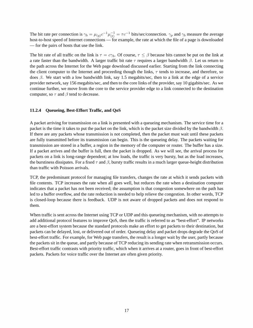
Figure1: Utilization, u, is graphed against log delay, log2(δ) given the delay probability, w, and the stream, i. .........................................................................................................25 Figure 2: Logit utilization, logit2(u), is graphed against log delay, log2(δ), given the delay probability, w, and the stream, i. ............................................................................27 Figure 3: Logit utilization, logit2(u), is graphed against the negative complementary log of the delay probability, ─ logit2(─logit2(w)), given the delay, δ, and the stream, i. ...........................................................................................................................28 Figure 4: Dotplot of median log connection bit rate, log2 (γb), for 6 Internet links. ......31 Figure 5: Dotplot of link median residuals from the first fit to the logit utilization using only the bit rate τ to characterize stream statistical properties. ........................................32 Figure 6: A partial residual plot for th eexplanatory variable for the Best-Effort DelayModel given each of the 6 Internet links. ........................................................................34 Figure 7: Dotplot of link median residuals for the Best-Effort Delay Model. ................35 Figure 8: The QoS utilization from the Best-Effort Delay Model is graphed against log delay given the bit rate and the delay probability. ....................................................36
iv

1 Overview: Introduction IP network technology cannot continue on an ever-increasing course o technological complexity and yet require the kind of human intervention that is necessary today for network management. Networks must be self-managing. This can only be done by a system of measurement that copes with the dynamics of packet movement. This system must process the packet-level measurements into variables that characterize network behaviors, which then form the basis for control algorithms that react to the variables. Such packet-level measurements can lead to characterization and control at the application layer, at the transport layer, at the network layer (including overlay networking), and in some cases at the link layer. This research will use tools of statistics, data mining and machine learning to explore packet-level measurement for self-management. The current dominant measurement framework on IP networks, SNMP, is not adequate to the task because it does not allow the determination of network time dynamics. We studied data that allows the determination of time dynamics—time-stamping the arrivals of packets at network nodes and recording header contents. The research used methods of statistics, data mining, and machine learning to: (1) determine network variables derivable from the measurements that characterize network behavior; (2) develop models of the critical network variables that characterize performance, usage, security, and early onset of problems; and (3) develop automated control methods based on the variables. In addition, certain models that we developed can provide traffic generation in network simulation systems
1

that can be used for further study of control.
Our project involved the study of previously collected packet header data on IP network links, as well asproviding for collection of new data.
The statistics, data mining, and machine learning was carried out using the S-Net software system for IPnetwork packet-level data. S-Net, the most comprehensive environment for packet header study availabletoday, was developed with support, in part, by DARPA under federal contract No. F30602-00-C-0034.
This report describes the work done under the above federal contract as well as previous work done underfederal contract No. F30602-02-2-C0093 awarded to Bell Labs because the work under the new contractwas a continuation of the work under the previous contract. In a later section of this final report the part ofthe work done under the new contract is described.
2 Overview: Main Elements of the Approach
Assembled a database of packet header data. Partnered with network operators who were a source not onlyof data, but provided knowledge of the critical network operations issues. Partnered with network equip-ment manufacturers to determine feasiblity of different packet-level measurement frameworks. Statisticalanalysis, data mining, and machine learning used to study network behavior using the S-Net system forpacket-header analysis and visualization. Developed models for the measurements. Developed algorithmsfor self-management based on the measurement scenario, models, and the learned network behavior.
3 Overview: Deliverables
1. Management and administration: As part of the conventional DARPA monthly reporting process,project management deliverables included the status of the effort, progress toward accomplishment of con-tract requirements, and monitoring funding use rates (spreadsheet format for financial reports with actualmonthly and cumulative expenditures compared with the programmed budget). We also made oral presen-tations at two DARPA PI meetings.
2. Research: Results on measurement frameworks, network characterization, models, variables that char-acterize network behavior, and self-managing control methods based on the variables, conveyed throughviewgraphs and written documents.
4 Overview: Statement of Work
We collaborated and cooperated with the other program contractors on the planning, design, implementationand demonstration of new technologies described within this proposal.
Over the course of execution of the contract resulting from this proposal, we maintained effective com-munications and active exchange with all other traffic modeling program researchers in order to facili-tate free-flowing information transfer and integration with other investigators. We actively exchanged re-search results with the larger research community through journal publications and oral presentations at
2

national/international seminars and meetings.
We documented technical work accomplished and information gained during performance of this acquisi-tion in the form of monthly status and special technical reports and this final report. These reports includedsignificant observations, problems, positive results, negative results, and design criteria. These reports doc-umented procedures followed, processes developed, lessons learned, and other useful information. Thereports documented the details of all technical work to permit full understanding of the techniques andprocedures used in evolving technology or processes developed.
Task 1: Packet-Level Measurement
We assembled a database of packet-level measurements consisting of packet header fields and time-stamps.The measurements were passive. We obtained existing measurements and deployed devices to collect moredata.
We studied best-effort traffic streams, the dominant traffic type on IP networks today, as well as voice overIP traffic. Increasingly, today’s voice traffic is moving from the circuit-switched telephone networks to IPnetworks. Many service providers now have architectures in which calls start and end on the circuit-switchednetworks, but are carried as IP network packet traffic over the IP network core. Very little measurement ofVoIP traffic has been carried out, a prerequisite to characterization and control. We obtained such data aspart of our study. For best-effort traffic the headers were IP and TCP (or UDP). For voice over IP traffic, theheaders were IP, UDP, and RTP.
Task 2: Statistical Analysis, Data Mining, and Machine Learning for Network Characterizationand Modeling
The data from our measurement plans were studied extensively in the S-Net environment. We determinedvariables that characterize network behavior and developed models for network traffic. The models canprovide traffic generation for network simulators.
Task 3: Automated Control
We developed an automated control method for network self-management based on the above variables fornetwork characterization. The performance of the control methods were studied through simulation methodsand analytical mathematical methods.
5 Overview: Key Personnel
1. Supported by Grant.
William S. Cleveland, Professor of Statistics and Professor of Computer Science, Purdue University
Michael Zhu, Assistant Professor of Statistics, Purdue University
Hui Chen, Graduate Student, Statistics Department, Purdue University
2. Substantial work was carried out by personnel not supported by the grant.
Bowei Xi, Assistant Professor of Statistics, Purdue University
3

Douglas Crabill, System Administrator, Statistics Department, Purdue University
Scott Ballew, Lead Network Administrator, Information Technology, Purdue University
Joerg Micheel, Head, Passive Measurement, National Laboratory for Applied Network Research
Jin Cao, Member of Technical Staff, Bell Labs
Thomas Telkamp, Director of Research and Advanced Development, Global Crossing
4

6 Summary of Technical Results: Data Collection
6.1 VoIP Collection
We deployed a monitor on a 100-megabit VoIP Ethernet link on the Global Crossing Network. The linkcarries VoIP traffic in two directions between a Sonus gateway and a first router on the GBLX IP network.The hardware is a 100-mbps Ethernet DAG network card that carries out measurement on the card and canmeasure at full line speed to provide highly accurate time stamps. The DAG card timestamps each packetand captures the IP/UDP/RTP headers. We collected data for 48 hours.
In addition, we obtained call detail records for each call during the first 24 hours of the packet trace. Thedetail records let us see unequivocally the caller and called directions, the destinations of the calls, andcategories of the nature of the call terminations. The call detail records provide information that aid greatlythe analysis of the packet traces.
6.2 Best-Effort Collection
We obtained a monitor from the National Laboratory for Applied Network Research (NLANR) for packettrace collection on the 1 gbps link that carries both directions of all traffic between the Purdue Universitycampus and the rest of the Internet. The high-end monitor is a linux box with a monitor operating systemtogether with a light PC in the box that can reboot the monitor operating system and allow increased remotemaintenance. The box also contains a 1-gbps DAG card that does timestamping and packet header capture.Joerg Micheel of NLANR flew to the West Lafayette campus to help Scott Ballew and Doug Crabill in theinstallation. By agreeing to become part of the NLANR measurement program, which means we allow datacollection in part for the NLANR database, the box and travel for Micheel was paid for by the NSF grantthat supports the NLANR program.
6.3 Database from Previous Collection Efforts
In addition, we built a database of best effort packet traces from 6 Internet links. This live stream databaseconsists of 349 streams, 90 sec or 5 min in duration, from 6 links that we name BELL, NZIX, AIX1, AIX2,MFN1, and MFN2. The measured streams have negligible delay on the link input router. The mean numberof simultaneous active connections, c, ranges from 49 connections to 18,976 connections. The traffic bitrate, τ , ranges from 1.00 megabits/sec to 348 megabits/sec.
BELL is a 100 megabit/sec link in Murray Hill, NJ, USA connecting a Bell Labs local network of about3000 hosts to the rest of the Internet. The transmission is half-duplex, so both directions, in and out, aremultiplexed and carried on the same link, and a stream is the multiplexing of both directions; but to keepthe variable c commensurate for all of the six links, the two directions for each connection is counted astwo. In this presentation we use 195 BELL traces, each 5 min in length. NZIX is the 100 megabit/secNew Zealand Internet exchange hosted by the ITS department at the University of Waikato, Hamilton, NewZealand, that served as a peering point among a number of major New Zealand Internet Service Providersat the time of data collection. All arriving packets from the input/output ports on the switch are mirrored,multiplexed, and sent to a port where they are measured. Because all connections have two directions at theexchange, each connection counts 2 as for BELL. In this presentation we use 84 NZIX traces, each 5 min in
5

length. AIX1 and AIX2 are two separate 622 megabit/sec OC12 packet-over-sonet links, each carrying onedirection of the traffic between NASA Ames and the MAE-West Internet exchange. In this presentation weuse 23 AIX1 and 23 AIX2 traces, each 90 sec in length. AIX1 and AIX2 streams were collected as part ofa project at the National Laboratory for Applied Network Research where the data are collected in blocksof 90 sec. MFN1 and MFN2 are two separate 2.5 gigabit/sec OC48 packet-over-sonet links on the networkof the service provider Metropolitan Fiber Network; each link carries one direction of traffic between SanJose, California, USA and Seattle, Washington, USA.
We also downloaded from NLANR data collected on the OC3 link that connects the University of Leipzignetwork to the rest of the Internet.
7 Summary of Technical Results: Statistical Analysis, Data Mining, andMachine Learning for Network Characterization and Modeling
7.1 Algorithms for Data Processing and Strategies of Analysis
We purchased and installed a high-end two-processor linux box for analysis, learning, mining, and modelingof the trace data. We installed the S-Net system for graphics and data analysis on the box.
Algorithms were written in C, Perl, and the S language for graphics and data analysis to process the VoIPmeasurements. The algorithms represent a a dataflow that progresses from raw packet trace files, to primaryand secondary UNIX flatfile databases, and then to S objects. Our analysis is carried out within the Senvironment to allow comprehensive study.
An important part of the strategy for study is time blocking. We broke the trace and CDR data into timeblocks, and applied the same analysis to all blocks. We used 5 minute blocks to guarantee stationarity oftraffic processes within each interval and to create object sizes that were not to large for efficient computa-tion.
7.2 Analysis for VoIP
We used tools of statistical analysis, data mining, and machine learning to study the characteristics of theVoIP packet trace data. Most important in this exploratory, or first-study phase, were a host of visualizationtools.
We discovered that there were a very large number of packet level calls with no CDR records. They are allvery short. We studied their characteristics to see if they had anomalous behavior. They spread out acrosstime and space in proportion to the calls with CDR records. We concluded that certain calls short enoughnot to generate revenue are not saved in the CDR records.
The study consisted of a wide range of topics involving the VoIP traffic characteristics and the qualityperformance of the Global Crossing system
• call arrival process, intensity and detailed statistical behavior
• call characteristics such as numbers of attempts (without connection) and connections, call durations,and detailed behavior of packet-level characteristics during ringing period vs. during talking period
6

• packet jitter
• aggregate packet traffic statistical properties of inter-arrival times and packet counts in 20 ms intervals
• silence suppression
A number of results came from our analysis.
• call inter-arrivals have to a very good approximation an exponential marginal distribution
• the call inter-arrivals have a small amount of short-term positive autocorrelation
• the call durations have a Pareto distribution, which breaks with the past exponential behavior, causedbecause today’s call contain faxes and computer logins, not just the voice conversations of the past
• a very large fraction of calls are call attempts
• patterns in the ringing make us believe we can develop a classification algorithm for determining theringing period
• the level of jitter is very low, about ±150µsec.
• the packet arrival process is long-range dependent, caused by the Pareto marginal distribution of thecall durations; these statistical properties play an important role in the automated control rules forbandwidth allocation that we are developing.
7.3 FSD Models for Best-Effort Traffic
The statistical properties of best-effort traffic, the packet arrival process, with its long-range dependence,has not reached a consensus with different camps arguing for different views.
Almost all analysis in the past has consisted of the study of counts of packet arrivals in a fixed interval oftime such as 1ms or 10 ms. This is not sufficient to understand the arrival process because moving to acount is an information reduction method to simplify analysis. Instead, we studied and modeled all of theinformation, the packet arrival times.
We developed a new class of models, fractional sum-difference (FSD) models, for the inter-arrival times.The FSD models, which are non-Gaussian and long-range dependent, provide excellent fits to the inter-arrivals. We carried out extensive validation to demonstrate this. Our models provide a bridge betweenthe different camps, explaining and integrating results on multifractal modeling, long-range dependence,fractional Brownian motion, and convergence to Poisson processes.
In addition, our models can be used for open-loop generation of background traffic in network simulators.This represents the first such generation that properly recreates the properties of real traffic.
Suppose xv for v = 1, 2, . . . is a stationary time series with marginal cumulative distribution functionF (x;φ) where φ is a vector of unknown parameters. Let x∗v = H(xv;φ) be a transformation of xv such thatthe marginal distribution of x∗v is normal with mean 0 and variance 1. We have H(xv;φ) = G−1(F (x;φ)),where G(z) is the cumulative distribution function of a normal random variable with mean 0 and variance1. Next we suppose x∗v is a Gaussian time series and call x∗v the “Gaussian image” of xv.
Suppose x∗v has the following form:
x∗v =√
1 − θ sv +√θ nv,
7

where sv and nv are independent of one another and each has mean 0 and variance 1. nv is Gaussian whitenoise, that is, an independent time series. sv is a Gaussian fractional ARIMA (Hosking 1981)
(I −B)dsv = εv + εu−1
where Bsv = su−1, 0 < d < 0.5, and εv is Gaussian white noise with mean 0 and variance
σ2ε =
(1 − d)Γ2(1 − d)
2Γ(1 − 2d).
xv is a fractional sum-difference (FSD) time series. Its Gaussian image, x∗v, has two components.√
1 − θsv
is the long-range-dependent, or lrd, component; its variance is 1 − θ.√θ is the white-noise component; its
variance is θ.
Let px∗(f) be the power spectrum of the x∗v. Then
px∗(f) = (1 − θ)σ2ε
4 cos2(πf)(
4 sin2(πf))d
+ θ
for 0 ≤ f ≤ 0.5. As f → 0.5, px∗(f) decreases monotonically to θ. As f → 0, px∗(f) goes to infinity likesin−2d(πf) ∼ f−2d, one outcome of long-range dependence. For nonnegative integer lags k, let rx∗(k),rs(k), and rn(k) be the autocovariance functions of x∗v, sv, and nv, respectively. Because the three serieshave variance 1, the autocovariance functions are also the autocorrelation functions. rs(k) is positive andfalls off like k2d−1 as k increases, another outcome of long-range dependence. For k > 0, rn(k) = 0 and
rx∗(k) = (1 − θ)rs(k).
As θ → 1, x∗v goes to white noise: px∗(f) → 1 and rx∗(k) → 0 for k > 0. The change in the autocovariancefunction and power spectrum are instructive. As θ gets closer to 1, the rise of px∗(f) near f = 0 is alwaysto order f−2d, and the rate of decay of rx∗(k) for large k is always k2d−1; but the ascent of px∗(f) at theorigin begins closer and closer to f = 0 and the rx∗(k) get uniformly smaller by the multiplicative factor1 − θ.
We model the marginal distribution of tv by a Weibull with shape λ and scale α, a family with two unknownparameters. Estimates of λ are almost always less than 1. The Weibull provides an excellent approximationof the sample marginal distribution of the tv except that the smallest 3% to 5% of the sample distribution istruncated to a nearly constant value due to certain network transmission properties.
The marginal distribution of qv is modeled as follows. While packets less than 40 bytes can occur, it issufficiently rare that we ignore this and suppose 40 ≤ qv ≤ 1500. First, we provide for A atoms at sizesφ
(s)1 . . . φ
(s)A such as 40 bytes, 512 bytes, 576 bytes, and 1500 bytes that are commonly occurring sizes; the
atom probabilities are φ(a)1 . . . φ
(a)A . For the remaining sizes, we divided the interval [40, 1500] bytes into
C sub-intervals using C − 1 distinct break points with values that are greater than 40 bytes and less than1500 bytes, φ(b)
1 , . . . φ(b)C−1. For each of the C sub-intervals, the size distribution has an equal probability
for the remaining sizes (excluding the atoms) in the sub-interval; the total probabilities for the sub-intervalsare φ(i)
1 , . . . , φ(i)C . Typically, with just 3 atoms at 40 bytes, 576 bytes, and 1500 bytes, and with just 2 break
points at 50 bytes and 200 bytes, we get an excellent approximation of the marginal distribution.
The transformed time series t∗v and q∗v appear to be quite close to Gaussian processes. Some small amountof non-Gaussian behavior is still present but it is minor. The autocorrelation structure of these Gaussianimages are very well fitted by the FSD autocorrelation structure.
8
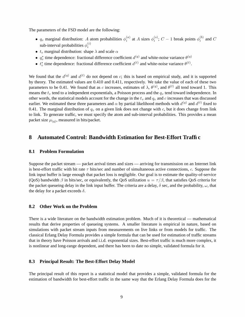
The parameters of the FSD model are the following:
• qv marginal distribution: A atom probabilities φ(a)i at A sizes φ(s)
i ; C − 1 break points φ(b)i and C
sub-interval probabilities φ(i)i
• tv marginal distribution: shape λ and scale α
• q∗v time dependence: fractional difference coefficient d(q) and white-noise variance θ(q)
• t∗v time dependence: fractional difference coefficient d(t) and white-noise variance θ(t).
We found that the d(q) and d(t) do not depend on c; this is based on empirical study, and it is supportedby theory. The estimated values are 0.410 and 0.411, respectively. We take the value of each of these twoparameters to be 0.41. We found that as c increases, estimates of λ, θ(q), and θ(t) all tend toward 1. Thismeans the tv tend to a independent exponentials, a Poisson process and the qv tend toward independence. Inother words, the statistical models account for the change in the tv and qv and c increases that was discussedearlier. We estimated these three parameters and α by partial likelihood methods with d(q) and d(t) fixed to0.41. The marginal distribution of qv on a given link does not change with c, but it does change from linkto link. To generate traffic, we must specify the atom and sub-interval probabilities. This provides a meanpacket size µ(q), measured in bits/packet.
8 Automated Control: Bandwidth Estimation for Best-Effort Traffic
8.1 Problem Formulation
Suppose the packet stream — packet arrival times and sizes — arriving for transmission on an Internet linkis best-effort traffic with bit rate τ bits/sec and number of simultaneous active connections, c. Suppose thelink input buffer is large enough that packet loss is negligible. Our goal is to estimate the quality-of-service(QoS) bandwidth β in bits/sec, or equivalently, the QoS utilization u = τ/β, that satisfies QoS criteria forthe packet queueing delay in the link input buffer. The criteria are a delay, δ sec, and the probability, ω, thatthe delay for a packet exceeds δ.
8.2 Other Work on the Problem
There is a wide literature on the bandwidth estimation problem. Much of it is theoretical — mathematicalresults that derive properties of queueing systems. A smaller literature is empirical in nature, based onsimulations with packet stream inputs from measurements on live links or from models for traffic. Theclassical Erlang Delay Formula provides a simple formula that can be used for estimation of traffic streamsthat in theory have Poisson arrivals and i.i.d. exponential sizes. Best-effort traffic is much more complex, itis nonlinear and long-range dependent, and there has been to date no simple, validated formula for it.
8.3 Principal Result: The Best-Effort Delay Model
The principal result of this report is a statistical model that provides a simple, validated formula for theestimation of bandwidth for best-effort traffic in the same way that the Erlang Delay Formula does for the
9

Poisson-exponential case. The model has been validated through extensive empirical study and throughconsistency with certain theoretical properties of queueing.
The model consists of the Best-Effort Delay Formula plus random variation:
logit2(u) = o+ oc log2(c) + oτδ log2(τδ) + oω(− log2(− log2(ω))) + ψ.
ψ is a random error variable with mean 0 and median absolute deviation mδ(ψ), which depends on δ; log2
is the log base 2; and logit2(u) = log2(u/(1 − u)). The distribution of 0.691ψ/mδ(ψ) is a t-distributionwith 15 degrees of freedom. Estimates of the coefficients of the model are
o = −8.933 oc = 0.420 oτδ = 0.444 oω = 0.893.
mδ(ψ) is modeled as a function of δ: log2(mδ(ψ)) is a linear function of log2(δ) plus random variation.The estimate of the intercept of the line is –0.481, the estimate of the linear coefficient of the line is 0.166,and the estimate of the standard error is 0.189. The bit rate τ is equal to cγb where γb is the connection bitrate in bits/sec/connection. So the Best-Effort Delay Formula can also be written as
logit2(u) = o+ (oc + oτδ) log2(c) + oτδ log2(γbδ) + oω(− log2(− log2(ω))).
In this form we see the action of the amount of multiplexing of connections as measured by c, and the end-to-end connection speed as measured by γb. An increase in either results in an increase in the utilization ofa link.
The Best-Effort Delay Model is used to estimate the bandwidth required to carry best-effort traffic given δ,ω, τ , and c. The QoS logit utilization is estimated by
ˆ= −8.933 + 0.420 log2(c) + .444 log2(τδ) + 0.893(− log2(− log2(ω))),
so the QoS utilization is estimated by
u =2
ˆ
1 + 2ˆ.
The corresponding estimated bandwidth is τ/u. For such an estimate there is a 50% chance of being toolarge and a 50% chance of being too small. We might however, use a more conservative estimate thatprovides a much smaller chance of too little bandwidth. Let
mδ(ψ) = 2−0.481+0.166 log2(δ)
be the estimate of m(δ). Let t15(p) be the lower 100p% percentage point of a t-distribution with 15 degreesof freedom, where p is small, say 0.05. Let
ˆ(p) = ˆ− m(δ)t15(p)/0.691
Then
u(p) =2
ˆ(p)
1 + 2ˆ(p),
is a conservative utilization estimate, the lower limit of a 100p% tolerance interval for the QoS utilization.The corresponding estimated bandwidth is τ/u(p).
10

8.4 Methods
The Best-Effort Delay Model was built, in part, from queueing theory. Certain predictor variables weresuggested by the Erlang Delay Formula. Theory prescribes certain behavior as τ , c, or γb increase, resultingin rate gains, multiplexing gains, or fast-forward invariance, and the model was constructed to reproduce thebehavior.
The Best-Effort Delay Model was built, in part, from results of queueing simulations with traffic streaminputs of two types, live and synthetic. The live streams are measurements of packet arrivals and sizes for349 intervals, 90 sec or 5 min in duration, from 6 Internet links. The synthetic streams are arrivals andsizes generated by recently developed FSD time series models for the arrivals and sizes of best-effort traffic.Each of the live streams was fitted by two FSD models, one for the inter-arrivals and one for the sizes, anda synthetic stream of 5 min was generated by the models. The generated inter-arrivals are independent ofthe generated sizes, which is what we found in the live data. The result is 349 synthetic streams that matchthe statistical properties collectively of the live streams. For each live or synthetic stream, we carried out25 runs, each with a number of simulations. For each run we picked a delay δ and a delay probability ω;simulations were carried out to find the QoS bandwidth β, the bandwidth that results in delay probabilityω for δ. This also yields a QoS utilization u = τ/β. We used 5 delays — 0.001 sec, 0.005 sec, 0.010sec, 0.050 sec, 0.100 sec — and 5 delay probabilities — 0.001, 0.005, 0.01, 0.02, and 0.05 — employingall 25 combinations of the two delay criteria. The queueing simulation results in delay data: values of fivevariables — QoS utilization u, delay δ, delay probability ω, the mean number of active connections of thetraffic c, and the traffic bit rate τ . The delay data were used in the model building.
8.5 Validity and Applicability
Extensive data exploration with visualization tools, some shown here, demonstrate that the Best-Effort DelayModel fits the simulation delay data. This, of course, is necessary for the model to be valid. In addition,validity is supported by the model reproducing the theoretical queueing properties as just discussed.
The validity of the Best-Effort Delay Model depends on the validity of the traffic streams used as inputsto the queueing simulation; that is, the packet streams must reproduce the statistical properties of best-effort streams. Of course, the live streams of the study do so because they are best-effort traffic. Extensivevalidation has shown that the FSD models, used to generate the packet streams here, provide excellent fitsto best-effort packet streams when c is above about 64 connections, which for a link where γb is about 214
bits/sec/connection means τ is above about 1 megabit/sec. For this reason, only traffic streams with τ greaterthan this rate are used in the study, and the Best-Effort Delay Model is valid above this rate.
The results are only valid for links with a large enough buffer that the packet loss is negligible. We haveused open-loop study, which does not provide for the TCP feedback that occurs when loss is significant.
There is also a practical restriction on applicability. We have taken the range of our study to include trafficbit rates as low as about 1 megabit/sec. We have done this simply because we can do so and achieve validresults. But even for the least stringent of our delay criteria, δ = 0.1 sec delay and ω = 0.05 delay probability,the utilizations are low for rates in the range of 1 megabit/sec to 5 megabits/sec. This might well be judgedto be too small a utilization to be practical; if so, it might mean that the what must be sacrificed is thenegligible packet loss, which means that a QoS study at the very low traffic bit rates needs to take accountof TCP feedback.
11

One outcome of the dependence of the bandwidth estimation on the traffic statistics is that our solution forbest-effort traffic would not apply to other forms of Internet traffic that do not share the best-effort statisticalproperties. One example is voice traffic.
Finally, the Best-Effort Delay Model provides an estimation of bandwidth in isolation without consideringother network factors. A major factor in network design is link failures. Redundancy needs to be built intothe system. So an estimate of bandwidth from the model for a link based on the normal link traffic may bereduced to provide the redundancy. But the model still plays a role because the bandwidth must be chosenbased on link traffic, but now the traffic in the event of a failure elsewhere.
9 Automated Control: Bandwidth Estimation for VoIP
Today, no automated methods exist for determining how many calls can be put on a VoIP link and maintainQoS criteria for delay and packet jitter. We designed a queueing simulation and modeling mechanism todetermine a statistical process-control approach that would allow automation provisioning of traffic on alink.
In the simulation, calls arrive as a Poisson process, a reasonable approximation to the observed behavior ofthe arrivals process. For each arrival, we sample with replacement from our call database, about 300,000calls, and use the observed packet process of each sampled call in the simulation.
In the simulation we fixed the traffic call rate and vary the link bandwidth (link speed) so that the utilizationranges from 30% to 99%, and study the resulting queueing delay and jitter of the packets. We built statisticalmodels for the delay and jitter based on the utilization, the number of simultaneous active calls and thebitrate. The models provide the requisite statistical process control.
We studied our simulation runs and discovered that there are instabilities when the utilization gets beyond acertain limit, which makes delay estimation problematic. The limit decreases and the traffic rate decreases.The phenomenon means the network cannot operate at these utilizations, so they are not relevant. We cannotleave them in the data to be modeled because they depart from standard conditions, so we will eliminatedthem from the study, using machine learning rules for the elimination.
10 Work Under The Current Contract
This report describes the work done under the above federal contract as well as previous work done underfederal contract No. F30602-02-2-C0093 awarded to Bell Labs because the work under the new contractwas a continuation of the work under the previous contract.
The following describes that portion of the work completed under the new contract:Task 1: Packet-Level Measurement
• Newark VoIP packet trace data collection and data processing
• Leipzig best-effort traffic processing
• installation of NLANR packet trace collector on Purdue Internet access link for best-effort trafficmeasurement
12
Task 2: Statistical Analysis, Data Mining, and Machine Learning for Network Characterization and Model-ing
• all analysis of the Newark VoIP data
• all work on the integration of best-effort traffic models through the understanding provided by thefractional sum-difference models
Task 3: Automated Control
• all simulations for bandwidth estimation for VoIP traffic and ensuing analysis and modeling of results
• simulations for best-effort traffic were completely redesigned and carried out, and new results ana-lyzed and modeled
11 Detailed Technical Report
11.1 Introduction: Contents of the Paper
The Internet is a world-wide computer network; at any given moment, a vast number of pairs of hosts aretransferring files one to the other. Each transferred file is broken up into packets that are sent along a pathacross the Internet consisting of links and nodes. The first node is the sending host; a packet exits the hostand travels along a link (fiber, wire, cable, or air) to a first router node, then over a link to a second routernode, and so forth until a last router sends the packet to a receiving host node over a final link.
The packet traffic arriving for transmission on an Internet link is a stream: a sequence of packets with arrivaltimes (sec) and sizes (bytes or bits). The packets come from pairs of hosts using the link for their transfers;that is, the link lies on the path from one host to another for each of a collection of pairs of hosts. When apacket arrives for transmission on a link, it enters a buffer (bits) where it must wait if there are other packetswaiting for transmission or if a packet is in service, that is, in the process of moving out of the buffer ontothe link. If the buffer is full, the packet is dropped.
A link has a bandwidth (bits/sec), the rate at which the bits of a packet are put on the link. Over an intervalof time during which the traffic is stationary, the packets arrive for transmission at a certain rate, the trafficbit rate (bits/sec), which is defined, formally, to be the mean of the packets sizes (bits) divided by the meanpacket inter-arrival time (sec), but this is approximately the mean number of arriving bits over the intervaldivided by the interval length (sec). Over the interval there is a mean simultaneous active connection load,the mean number of source-destination pairs of hosts actively sending packets over the link. The utilizationof the link is the traffic bit rate divided by the bandwidth; it measures the traffic rate relative to the capacityof the link.
This article presents results on a fundamental problem of engineering the Internet. What link bandwidth isneeded to accommodate traffic with a certain bit rate and ensure that the transmission on the link maintainsquality-of-service, or QoS, criteria? Finding the QoS bandwidth must be faced in setting up every link onthe Internet, from the low-bandwidth links connecting the computers of a home user to the high-bandwidthlinks of a major Internet service provider. Our approach to solving the bandwidth estimation problem is touse queueing theory and queueing simulations to build a model for the QoS bandwidth. The traffic inputsare live streams from measurements of live links and synthetic streams from statistical models for trafficstreams.
13

Section 11.2 describes Internet TCP/IP transmission technology, which governs almost all computer net-working today — for example, the networks of Internet service providers, universities, companies, andhomes. Section 11.2 also describes the buffer queueing process and its affect on the QoS of file transfer.
Section 11.3 formulates the particular version of the bandwidth estimation problem that is addressed here,discusses why the statistical properties of the packet streams are so critical to bandwidth estimation, andoutlines how we use queueing simulations to study the problem. We study “best-effort” Internet trafficstreams because they are the predominant type of traffic on Internet links today. The QoS criteria forbest-effort streams are the packet loss (fraction of lost packets), the queueing delay (sec), and the delayprobability (probability of a packet exceeding the delay). We suppose that the link packet loss is negligible,and find the QoS bandwidth required for a packet stream of a certain load that satisfies the delay and thedelay probability.
Section 11.4 describes fractional sum-difference (FSD) time series models, which are used to generate thesynthetic streams for the queueing simulations. The FSD models, a new class of non-Gaussian, long-rangedependent time series models, provide excellent fits to packet size time series and to packet inter-arrivaltime series. The validation of the FSD models is critical to this study. The validity of our solution to thebandwidth estimation problem depends on having traffic inputs to the queueing that reproduce the statisticalproperties of best-effort traffic. Of course, the live data have the properties, but we need assurance that thesynthetic data do as well.
Section 11.5 describes the live packet arrivals and sizes and the synthetic packet arrivals and sizes that aregenerated by the FSD models. Section 11.6 gives the details of the simulations and the resulting delay data:values of the QoS bandwidth, delay, delay probability, mean number of active host-pair connections of thetraffic, and traffic bit rate.
Model building, based on the simulation delay data and on queueing theory, begins in Section 11.7. Todo the model building and diagnostics, we exploit the structure of the delay data — utilizations for allcombinations of delay and delay probability for each stream, live or synthetic. We develop an initial modelthat relates, for each stream, the QoS utilization (bit rate divided by the QoS bandwidth) to the delay anddelay probability. We find a transformation for the utilization for which the functional dependence on thedelay and delay probability does not change with the stream. There is also an additive stream coefficientthat varies across streams, characterizing the statistical properties of each stream. This stream-coefficientdelay model cannot be used for bandwidth estimation because the stream coefficient would not be known inpractice.
Next we add two variables to the model that measure the statistical properties of the streams and that canbe specified or measured in practice — the traffic bit rate and the number of simultaneous active host-pairconnections on the link — and drop the stream coefficients. In effect we have modeled the coefficients.The result is the Best-Effort Delay Model: a Best-Effort Delay Formula for the utilization as a function of(1) the delay, (2) the delay probability, (3) the traffic bit rate, and (4) the mean number of active host-pairconnections of the traffic, plus a random error term.
Section 11.8 presents a method for bandwidth estimation that starts with the value from the Best-EffortDelay Formula, and then uses the error distribution of the Best-Effort Delay Model to find a toleranceinterval whose minimum value provides an conservative estimate with a low probability of being too small.
Section 11.9 discusses previous work on bandwidth estimation, and how it differs from the work here.Section 11.10 is an extended abstract. Readers who seek just results can proceed to this section; those notfamiliar with Internet engineering technology might want to first read Sections 11.2 and 11.3.
14

The following notation is used throughout the article:
Packet Stream
• v : arrival numbers (number) v = 1 is the first packet, v = 2 is the second packet, etc.
• av : arrival times (sec)
• tv : inter-arrival times (sec) tv = av+1 − av
• qv : sizes (bytes or bits).
Traffic Load
• c : mean number of simultaneous active connections (number)
• τ : traffic bit rate (bits/sec)
• γp : connection packet rate (packets/sec/connection)
• γb : connection bit rate (bits/sec/connection).
Bandwidth
• β : bandwidth (bits/sec)
• u : utilization (fraction) τ/β.
Queueing
• δ : packet delay (sec)
• ω : delay probability (fraction).
11.2 Internet Technology
The Internet is a computer network over which a pair of host computers can transfer one or more files (Stevens1994). Consider the downloading of a Web page, which is often made up of more than one file. One host, theclient, sends a request file to start the downloading of the page. Another host, the server, receives the requestfile and sends back a first response file; this process continues until all of the response files necessary todisplay the page are sent. The client passes the received response files to a browser such as Netscape, whichthen displays the page on the screen. This section gives information about some of the Internet engineeringprotocols involved in such file transfer.
11.2.1 Packet Communications
When a file is sent, it is broken up into packets whose sizes are 1460 bytes or less. The packets are sentfrom the source host to the destination host where they are reassembled to form the original file. They travelalong a path across the Internet that consists of transmission links and routers. The source computer isconnected to a first router by a transmission link; the first router is connected to a second router by anothertransmission link, and so forth. A router has input links and output links. When it receives a packet from oneof its input links, it reads the destination address on the packet, determines which of the routers connectedto it by output links should get the packet, and sends out the packet over the output link connected to that
15

router. The flight across the Internet ends when a final router receives the packet on one of its input linksand sends the packet to the destination computer over one of its output links.
The two hosts establish a connection to carry out one or more file transfers. The connection consists ofsoftware running on the two computers that manages the sending and receiving of packets. The softwareexecutes an Internet transport protocol, a detailed prescription for how the sending and receiving shouldwork. The two major transport protocols are UDP and TCP. UDP just sends the packets out. With TCP,the two hosts exchange control packets that manage the connection. TCP opens the connection, closes it,retransmits packets not received by the destination, and controls the rate at which packets are sent based onthe amount of retransmission that occurs. The transport software adds a header to each packet that containsinformation about the file transfer. The header is 20 bytes for TCP and 8 bytes for UDP.
Software running on the two hosts implements another network protocol, IP (Internet Protocol), that man-ages the involvement of the two hosts in the routing of a packet across the Internet. The software adds a20-byte IP header to the packet with information needed in the routing such as the source host IP addressand the destination host IP address. IP epitomizes the conceptual framework that underlies Internet packettransmission technology. The networks that make up the Internet — for example, the networks of Internetservice providers, universities, companies, and homes — are often referred to as IP networks, although todayit is unnecessary because almost all computer networking is IP, a public-domain technology that defeatedall other contenders, including the proprietary systems of big computer and communications companies.
11.2.2 Link Bandwidth
The links along the path between the source and destination hosts each have a bandwidth β in bits/sec. Thebandwidth refers to the speed at which the bits of a packet are put on the link by a computer or router. For thelink connecting a home computer to a first router, β might be 56 kilobits/sec if the computer uses an internalmodem, or 1.5 megabits/sec if there is a broadband connection, a cable or DSL link. The link connecting auniversity computer to a first router might be 10 megabits/sec, 100 megabits/sec, or 1 gigabit/sec. The linkson the core network of a major Internet service provider have a wide range of bandwidths; typical valuesrange from 45 megabits/sec to 10 gigabits/sec. For a 40 byte packet, which is 320 bits, it takes 5.714 msto put the packet on a 56 kilobit/sec link, and 0.032 µs to put it on a 10 gigabits/sec link, which is about180,000 times faster. Once a bit is put on the link, it travels down the link at the speed of light.
11.2.3 Active Connections, Statistical Multiplexing, and Measures of Traffic Loads
At any given moment, an Internet link has a number of simultaneous active connections; this is the numberof pairs of computers connected with one another that are sending packets over the link. The packets ofthe different connections are intermingled on the link; for example, if there are three active connections, thearrival order of 10 consecutive packets by connection number might be 1, 1, 2, 3, 1, 1, 3, 3, 2, and 3. Theintermingling is referred to as “statistical multiplexing”. On a link that connects a local network with about500 users there might be 300 active connections during a peak period. On the core link of an Internet serviceprovider there might be 60,000 active connections.
During an interval of time when the traffic is stationary, there is a mean number of active connections c, anda traffic bit rate τ in bits/sec. Let µ(t) in sec be the mean packet inter-arrival time, and let µ(q), in bits, bethe mean packet size. Then the packet arrival rate per connection is γp = c−1µ−1
(t) packets/sec/connection.
16
The bit rate per connection is γb = µ(q)c
−1µ−1(t) = τc−1 bits/sec/connection. γp and γb measure the average
host-to-host speed of Internet connections — for example, the rate at which the file of a page is downloaded— for the pairs of hosts that use the link.
The bit rate of all traffic on the link is τ = cγb. Of course, τ ≤ β because bits cannot be put on the link ata rate faster than the bandwidth. A larger traffic bit rate τ requires a larger bandwidth β. Let us return tothe path across the Internet for the Web page download discussed earlier. Starting from the link connectingthe client computer to the Internet and proceeding though the links, τ tends to increase, and therefore, sodoes β. We start with a low bandwidth link, say 1.5 megabits/sec, then to a link at the edge of a serviceprovider network, say 156 megabits/sec, and then to the core links of the provider, say 10 gigabits/sec. As wecontinue further, we move from the core to the service provider edge to a link connected to the destinationcomputer, so τ and β tend to decrease.
11.2.4 Queueing, Best-Effort Traffic, and QoS
A packet arriving for transmission on a link is presented with a queueing mechanism. The service time for apacket is the time it takes to put the packet on the link, which is the packet size divided by the bandwidth β.If there are any packets whose transmission is not completed, then the packet must wait until these packetsare fully transmitted before its transmission can begin. This is the queueing delay. The packets waiting fortransmission are stored in a buffer, a region in the memory of the computer or router. The buffer has a size.If a packet arrives and the buffer is full, then the packet is dropped. As we will see, the arrival process forpackets on a link is long-range dependent; at low loads, the traffic is very bursty, but as the load increases,the burstiness dissipates. For a fixed τ and β, bursty traffic results in a much larger queue-height distributionthan traffic with Poisson arrivals.
TCP, the predominant protocol for managing file transfers, changes the rate at which it sends packets withfile contents. TCP increases the rate when all goes well, but reduces the rate when a destination computerindicates that a packet has not been received; the assumption is that congestion somewhere on the path hasled to a buffer overflow, and the rate reduction is needed to help relieve the congestion. In other words, TCPis closed-loop because there is feedback. UDP is not aware of dropped packets and does not respond tothem.
When traffic is sent across the Internet using TCP or UDP and this queueing mechanism, with no attempts toadd additional protocol features to improve QoS, then the traffic is referred to as “best-effort”. IP networksare a best-effort system because the standard protocols make an effort to get packets to their destination, butpackets can be delayed, lost, or delivered out of order. Queueing delay and packet drops degrade the QoS ofbest-effort traffic. For example, for Web page transfers, the result is a longer wait by the user, partly becausethe packets sit in the queue, and partly because of TCP reducing its sending rate when retransmission occurs.Best-effort traffic contrasts with priority traffic, which when it arrives at a router, goes in front of best-effortpackets. Packets for voice traffic over the Internet are often given priority.
17

11.3 The Bandwidth Estimation Problem: Formulation and Stream Statistical Properties
11.3.1 Formulation
Poor QoS resulting from delays and drops on an Internet link can be improved by increasing the link band-width β. The service time decreases, so if the traffic rate τ remains fixed, the queuing delay distributiondecreases, and delay and loss are reduced. Loss and delay are also affected by the buffer size; the largerthe buffer size, the fewer the drops, but then the queueing delay has the potential to increase because themaximum queueing delay is the buffer size divided by β.
The bandwidth estimation problem is to choose β to satisfy QoS criteria. The resulting value of β is theQoS bandwidth. The QoS utilization is the value of u = τ/β corresponding to the QoS bandwidth. Whena local network, such as a company or university, purchases bandwidth from an Internet service provider, adecision on β must be made. When an Internet service provider designs its network, it must choose β foreach of its links. The decision must be based on the traffic load and QoS criteria.
Here, we address the bandwidth estimation problem specifically for links with best-effort traffic. We takethe QoS criteria to be delay and loss. For delay, we use two metrics: a delay, δ, and the delay probability,ω, the probability that a packet exceeds the delay. For loss, we suppose that the decision has been madeto choose a buffer size large enough that drops will be negligible. This is, for example, consistent withthe current practice of service providers on their core links (Iyer, Bhattacharyya, Taft, McKeown, and Diot2003). Of course, a large buffer size allows the possibility of a large delay, but setting QoS values for δand ω allows us to control delay probabilistically; we will chose ω to be small. The alternative is to use thebuffer size as a hard limit on delay, but because dropped packets are an extreme remedy with more seriousdegradations of QoS, it is preferable to separate loss and delay control, using the softer probabilistic controlfor delay. Stipulating that packet loss will be negligible on the link means that for a connection that uses thelink, another link will be the loss bottleneck; that is, if packets of the connection are dropped, it will be onanother link. It also means that TCP feedback can be ignored in studying the bandwidth estimation problem.
11.3.2 Packet Stream Statistical Properties
A packet stream consists of a sequence of arriving packets, each with a size. Let v be the arrival number; v=1 is the first packet, v = 2 is the second packet, and so forth. Let av be the arrival times, let tv = av+1 − av
be the inter-arrival times, and let qv be the size of the packet arriving at time av. The statistical properties ofthe packet stream will be described by the statistical properties of tv and qv as time series in v.
The QoS bandwidth for a packet stream depends critically on the statistical properties of the tv and qv.Directly, the bandwidth depends on the queue-length time process. But the queue-length time processdepends critically on the stream statistical properties. Here, we consider best-effort traffic. It has persistent,long-range dependent tv and qv (Ribeiro, Riedi, Crouse, and Baraniuk 1999; Gao and Rubin 2001; Cao,Cleveland, Lin, and Sun 2001). Persistent, long-range dependent tv and qv have dramatically larger queue-size distributions than those for independent tv and qv (Konstantopoulos and Lin 1996; Erramilli, Narayan,and Willinger 1996; Cao, Cleveland, Lin, and Sun 2001). The long-range dependent traffic is burstier thanthe independent traffic, so the QoS utilization is smaller because more headroom is needed to allow forthe bursts. This finding demonstrates quite clearly the impact of the statistical properties. But a corollaryof the finding is that the results here are limited to best-effort traffic streams (or any other streams withsimilar statistical properties). Results for other types of traffic with quite different statistical properties —
18

for example, links carrying voice traffic using current Internet protocols — are different.
Best-effort traffic is not homogeneous. As the traffic connection load c increases, the arrivals tend towardPoisson and the sizes tend toward independent(Cao, Cleveland, Lin, and Sun 2002; Cao and Ramanan 2002).The reason is the increased statistical multiplexing of packets from different connections; the interminglingof the packets of different connections is a randomization process that breaks down the correlation of thestreams. In other words, the long-range dependence dissipates. This means that in our bandwidth estimationstudy, we can expect a changing estimation mechanism as c increases. In particular, we expect “multiplexinggains”, greater utilization due to the reduction in dependence. Because of the change in properties with c,we must be sure to study streams with a wide range of values of c.
11.4 FSD Time Series Models for Packet Arrivals and Sizes
This section presents FSD time series models, a new class of non-Gaussian, long-range dependent mod-els (Cao, Cleveland, Lin, and Sun 2002; Cao, Cleveland, and Sun 2004). The two independent packet-streamtime series — the inter-arrivals, tv, and the sizes, qv — are each modeled by an FSD model; the models areused to generate synthetic best-effort traffic streams for the queueing simulations of our study.
There are a number of known properties of the tv and qv that had to be accommodated by the FSD models.First, these two time series are long-range dependent. This is associated with the important discoveryof long-range dependence of packet arrival counts and of packet byte counts in successive equal-lengthintervals of time, such as 10 ms (Leland, Taqqu, Willinger, and Wilson 1994; Paxson and Floyd 1995).Second, the tv and qv are non-Gaussian. The complex non-Gaussian behavior has been demonstrated clearlyin important work showing that highly nonlinear multiplicative multi-fractal models can account for thestatistical properties of tv and qv (Riedi, Crouse, Ribeiro, and Baraniuk 1999; Gao and Rubin 2001). Thesenonparametric models utilize many coefficients and a complex cascade structure to explain the properties.Third, the statistical properties of the two time series change as c increases (Cao, Cleveland, Lin, and Sun2002). The arrivals tend toward Poisson and the sizes tend toward independent; there are always long-rangedependent components present in the series, but the contributions of the components to the variances of theseries goes to zero.
11.4.1 Solving the Non-Gaussian Challenge
The challenge in modeling tv and qv is their combined non-Gaussian and long-range dependent properties,a difficult combination that does not, without a simplifying approach, allow parsimonious characterization.We discovered that monotone nonlinear transformations of the inter-arrivals and sizes are very well fitted byparsimonious Gaussian time series, a very simple class of fractional ARIMA models (Hosking 1981) witha small number of parameters. In other words, the transformations and the Gaussian models account for thecomplex multifractal properties of the tv and the qv in a simple way.
11.4.2 The FSD Model Class
Suppose xv for v = 1, 2, . . . is a stationary time series with marginal cumulative distribution functionF (x;φ) where φ is a vector of unknown parameters. Let x∗v = H(xv;φ) be a transformation of xv such thatthe marginal distribution of x∗v is normal with mean 0 and variance 1. We have H(xv;φ) = G−1(F (x;φ)),
19

where G(z) is the cumulative distribution function of a normal random variable with mean 0 and variance1. Next we suppose x∗v is a Gaussian time series and call x∗v the “Gaussian image” of xv.
Suppose x∗v has the following form:
x∗v =√
1 − θ sv +√θ nv,
where sv and nv are independent of one another and each has mean 0 and variance 1. nv is Gaussian whitenoise, that is, an independent time series. sv is a Gaussian fractional ARIMA (Hosking 1981)
(I −B)dsv = εv + εu−1
where Bsv = su−1, 0 < d < 0.5, and εv is Gaussian white noise with mean 0 and variance
σ2ε =
(1 − d)Γ2(1 − d)
2Γ(1 − 2d).
xv is a fractional sum-difference (FSD) time series. Its Gaussian image, x∗v, has two components.√
1 − θsv
is the long-range-dependent, or lrd, component; its variance is 1 − θ.√θ is the white-noise component; its
variance is θ.
Let px∗(f) be the power spectrum of the x∗v. Then
px∗(f) = (1 − θ)σ2ε
4 cos2(πf)(
4 sin2(πf))d
+ θ
for 0 ≤ f ≤ 0.5. As f → 0.5, px∗(f) decreases monotonically to θ. As f → 0, px∗(f) goes to infinity likesin−2d(πf) ∼ f−2d, one outcome of long-range dependence. For nonnegative integer lags k, let rx∗(k),rs(k), and rn(k) be the autocovariance functions of x∗v, sv, and nv, respectively. Because the three serieshave variance 1, the autocovariance functions are also the autocorrelation functions. rs(k) is positive andfalls off like k2d−1 as k increases, another outcome of long-range dependence. For k > 0, rn(k) = 0 and
rx∗(k) = (1 − θ)rs(k).
As θ → 1, x∗v goes to white noise: px∗(f) → 1 and rx∗(k) → 0 for k > 0. The change in the autocovariancefunction and power spectrum are instructive. As θ gets closer to 1, the rise of px∗(f) near f = 0 is alwaysto order f−2d, and the rate of decay of rx∗(k) for large k is always k2d−1; but the ascent of px∗(f) at theorigin begins closer and closer to f = 0 and the rx∗(k) get uniformly smaller by the multiplicative factor1 − θ.
11.4.3 Marginal Distributions of qv and tv
We model the marginal distribution of tv by a Weibull with shape λ and scale α, a family with two unknownparameters. Estimates of λ are almost always less than 1. The Weibull provides an excellent approximationof the sample marginal distribution of the tv except that the smallest 3% to 5% of the sample distribution istruncated to a nearly constant value due to certain network transmission properties.
The marginal distribution of qv is modeled as follows. While packets less than 40 bytes can occur, it issufficiently rare that we ignore this and suppose 40 ≤ qv ≤ 1500. First, we provide for A atoms at sizes
20

φ(s)1 . . . φ
(s)A such as 40 bytes, 512 bytes, 576 bytes, and 1500 bytes that are commonly occurring sizes; the
atom probabilities are φ(a)1 . . . φ
(a)A . For the remaining sizes, we divided the interval [40, 1500] bytes into
C sub-intervals using C − 1 distinct break points with values that are greater than 40 bytes and less than1500 bytes, φ(b)
1 , . . . φ(b)C−1. For each of the C sub-intervals, the size distribution has an equal probability
for the remaining sizes (excluding the atoms) in the sub-interval; the total probabilities for the sub-intervalsare φ(i)
1 , . . . , φ(i)C . Typically, with just 3 atoms at 40 bytes, 576 bytes, and 1500 bytes, and with just 2 break
points at 50 bytes and 200 bytes, we get an excellent approximation of the marginal distribution.
11.4.4 Gaussian Images of qv and tv
The transformed time series t∗v and q∗v appear to be quite close to Gaussian processes. Some small amountof non-Gaussian behavior is still present but it is minor. The autocorrelation structure of these Gaussianimages are very well fitted by the FSD autocorrelation structure.
The parameters of the FSD model are the following:
• qv marginal distribution: A atom probabilities φ(a)i at A sizes φ(s)
i ; C − 1 break points φ(b)i and C
sub-interval probabilities φ(i)i
• tv marginal distribution: shape λ and scale α• q∗v time dependence: fractional difference coefficient d(q) and white-noise variance θ(q)
• t∗v time dependence: fractional difference coefficient d(t) and white-noise variance θ(t).
We found that the d(q) and d(t) do not depend on c; this is based on empirical study, and it is supportedby theory. The estimated values are 0.410 and 0.411, respectively. We take the value of each of these twoparameters to be 0.41. We found that as c increases, estimates of λ, θ(q), and θ(t) all tend toward 1. Thismeans the tv tend to a independent exponentials, a Poisson process and the qv tend toward independence. Inother words, the statistical models account for the change in the tv and qv and c increases that was discussedearlier. We estimated these three parameters and α by partial likelihood methods with d(q) and d(t) fixed to0.41. The marginal distribution of qv on a given link does not change with c, but it does change from linkto link. To generate traffic, we must specify the atom and sub-interval probabilities. This provides a meanpacket size µ(q), measured in bits/packet.
11.5 Packet Stream Data: Live and Synthetic
We use packet stream data, values of packet arrivals and sizes, in studying the bandwidth estimation problem.They are used as input traffic for queueing simulations. There are two types of streams: live and synthetic.The live streams are from packet traces, data collection from live Internet links. The synthetic streams aregenerated by the FSD models.
11.5.1 Live Packet Streams
A commonly-used measurement framework for empirical Internet studies results in packet traces (Claffy,Braun, and Polyzos 1995; Paxson 1997; Duffield, Feldmann, Friedmann, Greenberg, Greer, Johnson, Kalmanek,B.Krishnamurthy, Lavelle, Mishra, Ramakrishnan, Rexford, True, , and van der Merwe 2000). The arrival
21

time of each packet on a link is recorded and the contents of the headers are captured. The vast majority ofpackets are transported by TCP, so this means most headers have 40 bytes, 20 for TCP and 20 for IP. The livepacket traffic is measured by this mechanism over an interval; the time-stamps provide the live inter-arrivaltimes, tv, and the headers contain information that provides the live sizes, qv; so for each trace, there is astream of live arrivals and sizes.
The live stream database used in this presentation consists of 349 streams, 90 sec or 5 min in duration, from6 Internet links that we name BELL, NZIX, AIX1, AIX2, MFN1, and MFN2. The measured streams havenegligible delay on the link input router. The mean number of simultaneous active connections, c, rangesfrom 49 connections to 18,976 connections. The traffic bit rate, τ , ranges from 1.00 megabits/sec to 348megabits/sec.
BELL is a 100 megabit/sec link in Murray Hill, NJ, USA connecting a Bell Labs local network of about3000 hosts to the rest of the Internet. The transmission is half-duplex, so both directions, in and out, aremultiplexed and carried on the same link, and a stream is the multiplexing of both directions; but to keep thevariable c commensurate for all of the six links, the two directions for each connection is counted as two. Inthis presentation we use 195 BELL traces, each 5 min in length. NZIX is the 100 megabit/sec New ZealandInternet exchange hosted by the ITS department at the University of Waikato, Hamilton, New Zealand, thatserved as a peering point among a number of major New Zealand Internet Service Providers at the time ofdata collection (http://wand.cs.waikato.ac.nz/wand/wits/nzix/2/ ). All arriving packets from the input/outputports on the switch are mirrored, multiplexed, and sent to a port where they are measured. Because allconnections have two directions at the exchange, each connection counts 2 as for BELL. In this presentationwe use 84 NZIX traces, each 5 min in length. AIX1 and AIX2 are two separate 622 megabit/sec OC12packet-over-sonet links, each carrying one direction of the traffic between NASA Ames and the MAE-WestInternet exchange. In this presentation we use 23 AIX1 and 23 AIX2 traces, each 90 sec in length. AIX1 andAIX2 streams were collected as part of a project at the National Laboratory for Applied Network Researchwhere the data are collected in blocks of 90 sec (http://pma.nlanr.net/PMA ). MFN1 and MFN2 are twoseparate 2.5 gigabit/sec OC48 packet-over-sonet links on the network of the service provider MetropolitanFiber Network; each link carries one direction of traffic between San Jose, California, USA and Seattle,Washington, USA. In this presentation we use 12 MFN1 and 12 MFN2 traces, each 5 min in length.
The statistical properties of streams, as we have stated, depend on the connection load c, so it is importantthat the time interval of a live stream be small enough that c does not vary appreciably over the interval. Forany link, there is diurnal variation, a change in c with the time of day due to changes in the number of users.We chose 5 minutes to be the upper bound of the length of each stream to ensure stationarity. BELL, NXIZ,MFN1, and MFN2 streams are 5 min. AIX1 and AIX2 traces are 90 sec because the sampling plan at thesesites consisted of noncontiguous 90-sec intervals.
11.5.2 Synthetic Packet Streams
The synthetic streams are arrivals and sizes generated by the FSD models for tv and qv. Each of the livestreams is fitted by two FSD models, one for the tv and one for the qv, and a synthetic stream of 5 min isgenerated by the models. The generated tv are independent of the generated qv, which is what we found inthe live data. The result is 349 synthetic streams that match the statistical properties collectively of the livestreams.
22

11.6 Queueing Simulation
We study the bandwidth estimation problem through queueing simulation with an infinite buffer and a first-in-first-out queueing discipline. The inputs to the queues are the arrivals and sizes of the 349 live and 349synthetic packet streams described in Section 11.5.
For each live or synthetic stream, we carry out 25 runs, each with a number of simulations. For each runwe pick a delay δ and a delay probability ω; simulations are carried out to find the QoS bandwidth β, thebandwidth that results in delay probability ω for the delay δ. This also yields a QoS utilization u = τ/β.We use 5 delays — 0.001 sec, 0.005 sec, 0.010 sec, 0.050 sec, 0.100 sec — and 5 delay probabilities —0.001, 0.005, 0.01, 0.02, and 0.05 — employing all 25 combinations of the two delay criteria. For eachsimulation of a collection, δ is fixed a priori. We measure the queueing delay at the arrival times of thepackets, which determines the simulated queueing delay process. From the simulated process we find thedelay probability for the chosen δ. We repeat the simulation, changing the trial QoS bandwidth, until theattained delay probability approximately matches the chosen delay probability ω. The optimization is easybecause ω decreases as the trial QoS bandwidth increases for fixed δ.
In the optimization, we do not allow the utilization to go above 0.97; in other words, if the true QoS uti-lization is above 0.97, we set it to 0.97. The reason is that we use the logit scale, log(u/(1 − u)), in themodeling; above about 0.97, the scale becomes very sensitive to model mis-specification and the accuracyof the simulation, even though the utilizations above 0.97 for practical purposes are nearly equal. Similarly,we limit the lower range of the utilizations to be 0.05.
The result of the 25 runs for each of the 349 live and 349 synthetic streams is 25 measurements, one per run,of each of five variables: QoS utilization u, delay δ, delay probability ω, mean number of active connectionsc, and bit rate τ . The first three variables vary from run to run; the last two variables are the same for the 25runs for a stream because they measure the stream statistical properties. By design, the range of δ is 0.001sec to 0.100 sec, and the range of ω is 0.001 to 0.05. The range of the QoS utilizations is 0.05 to 0.97. Thetwo additional variables τ and c, which measure the statistical properties of the streams, are constant acrossthe 25 runs for each stream. c ranges from 49 connections to 18,976 connections, and τ ranges from 1.00megabits/sec to 348 megabits/sec.
11.7 Model Building: A Bandwidth Formula Plus Random Error
This section describes the process of building the Best-Effort Delay Model, which is the Best-Effort DelayFormula plus random error. The model describes the dependence of the utilization u on the delay δ, thedelay probability ω, the traffic bit rate τ , and the expected number of active connections c. The modelingprocess involves both theory and empirical study, and establishes a basis for the model.
The theoretical basis is queueing theory. The empirical basis is the delay data from the queueing simulations,the measurements of the five variables described in Section 11.6. The following notation is used for thevalues of these five variables for either the live delay data or the synthetic delay data. δj , for j = 1 to 5, arethe 5 values of the delay in increasing order, and ωk, for k =1 to 5, are the 5 values of the delay probabilityin increasing order. uijk is the QoS utilization for delay δj , delay probability ωk, and stream i, where i = 1to 349. τi is the traffic bit rate and ci is the mean number of active connections, both for stream i.
23

11.7.1 Strategy: Initial Modeling of Dependence on δ and ω
The structure of the data provides an opportunity for careful initial study of the dependency of the uijk on δjand ωk. We have 25 measurements of each of these variables for each stream i, and for these measurements,both τi and ci are constant. We start our model building by exploiting this opportunity.
We will consider modeling each stream separately, but hope there will be model consistency across streamsthat allows simplification. If such simplicity is to occur, it is likely that it will require a monotone trans-formation of the uijk because they vary between 0 and 1. So we begin, conceptually, with a model of theform
f(uijk) = gi(δj , ωk) + εijk.
The εijk are a sample from a distribution with mean 0. f is a monotone function of u, and gi is a functionof δ and ω; we want to choose f to make gi as simple as possible, that is, vary as little as possible with i.
11.7.2 Conditional Dependence of u on δ
We start our exploration of the data by taking f(u) = u and suppose that a logical scale for δ is the log. Inall cases, we use log base 2 and indicate this by writing log2 in our formulas. We do not necessarily believethat this identity function for f is the right transformation, but it is helpful to study the data initially on theuntransformed utilization scale.
Our first step is to explore the conditional dependence of uijk on log2(δj) given ωk and the stream i bytrellis display (Becker, Cleveland, and Shyu 1996). For each combination of the delay probability ωk andthe stream i, we graph uijk against log2(δj). We did this once for all 349 live streams and once for all 349synthetic streams. Figure 1 illustrates this by a trellis display for 16 of the live streams. The 16 streams werechosen to nearly cover the range of values of the τi. Let τ(v), for v = 1 to 349, be the values ordered fromsmallest to largest, and take τ(v) to be the quantile of the empirical distribution of the values of order v/349.Then we chose the 16 streams whose ranks v yield orders the closest to the 16 equally-spaced orders from0.05 to 0.95. On the figure, there are 80 panels divided into 10 columns and 8 rows. On each panel, uijk isgraphed against log2(δj) for one value of ωk and one stream; the strip labels at the top of each panel givethe value of ωk and the rank of the stream. There are 5 points per panel, one for each value of log2(δj).
Figure 1 shows a number of overall effects of τ , δ, and ω on u. For each pair of values of ω and τ , there isan increase in u with δ, a strong main effect in the data. In addition, there is an increase with τ for fixed δand ω, another strong main effect. There is also a main effect for ω, but smaller in magnitude than for theother two variables. The dependence of u on log2(δ) is nonlinear, and changes substantially with the valueof τ ; as τ increases, the overall slope in u as function of log2(δ) first increases and then decreases. In otherwords, there is an interaction between log2(δ) and τ . Such an interaction complicates the dependence, sowe search further for a transformation f of u that removes the interaction. This pattern occurs when all ofthe live streams or all of the synthetic streams are plotted in the same way.
There is an interaction between log2(δ) and τ in part because once u is close to 1, where there is littleroom for change as a function of log2(δ). For this reason, we tried expanding the scale at 1 by taking thefunction f(u) = log2(1 − u). This did not achieve appreciably greater simplicity because nonlinearity andan interaction are still strongly present, but the interaction cause is behavior for smaller values of τ .
The nature of the remaining interaction for f(u) = log2(1 − u) suggests that a logit transformation might
24
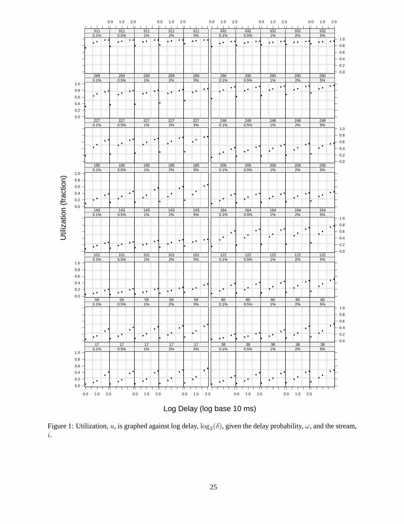
. ....
0.0
0.2
0.4
0.6
0.8
1.00.1%
17
0.0 1.0 2.0
. ....
0.5%17
. ....
1%17
0.0 1.0 2.0
. ....
2%17
. ....
5%17
0.0 1.0 2.0
. .. ..
0.1%38
. .. ..
0.5%38
0.0 1.0 2.0
. ....
1%38
. ....
2%38
0.0 1.0 2.0
. .. ..
5%38
. .. ..
0.1%59
. .. ..
0.5%59
. ....
1%59
. ....
2%59
. ....
5%59
. .. ..
0.1%80
. .. ..
0.5%80
. .. ..
1%80
. ....
2%80
. ....
0.0
0.2
0.4
0.6
0.8
1.05%80
. .. ..0.0
0.2
0.4
0.6
0.8
1.00.1%101
. .. ..
0.5%101
. .. ..
1%101
. .. ..
2%101
. .. ..
5%101
. .. ..
0.1%122
. .. ..
0.5%122
. .. ..
1%122
. .. ..
2%122
. .. ..
5%122
. .. ..
0.1%143
. .. ..
0.5%143
. .. ..
1%143
. .. ..
2%143
. .. ..
5%143
. ....
0.1%164
...
..0.5%164
...
..1%164
...
..2%164
...
..
0.0
0.2
0.4
0.6
0.8
1.05%164
. .. ..0.0
0.2
0.4
0.6
0.8
1.00.1%185
. .. ..
0.5%185
. ....
1%185
. ....
2%185
. ....
5%185
. .. ..
0.1%206
. .. ..
0.5%206
. .. ..
1%206
. .. ..
2%206
. .. ..
5%206
... ..0.1%227
... ..0.5%227
... ..
1%227
... ..
2%227
... ..
5%227
. .. ..
0.1%248
. .. ..
0.5%248
. .. ..
1%248
. .. ..
2%248
. .. ..
0.0
0.2
0.4
0.6
0.8
1.05%248
... ..
0.0
0.2
0.4
0.6
0.8
1.00.1%269
... ..0.5%269
... ..
1%269
... ..
2%269
... ..
5%269
... ..0.1%290
. .. ..0.5%290
. .. ..1%290
. .. ..2%290
. .. ..5%290
. .. ..0.1%311
. .. ..0.5%311
0.0 1.0 2.0
. .. ..1%311
. .. ..2%311
0.0 1.0 2.0
. .. ..5%311
. .. ..0.1%332
0.0 1.0 2.0
. .. ..0.5%332
. .. ..1%332
0.0 1.0 2.0
. .. ..2%332
. .. ..
0.0
0.2
0.4
0.6
0.8
1.05%332
0.0 1.0 2.0
Log Delay (log base 10 ms)
Util
izat
ion
(fra
ctio
n)
Figure 1: Utilization, u, is graphed against log delay, log2(δ), given the delay probability, ω, and the stream,i.
25

do better:
f(u) = logit2(u) = log2
(
u
1 − u
)
.
Figure 2 plots logit2(uijk) against log2(δj) using the same streams and method as Figure 1. The logitfunction greatly simplifies the dependence. The dependence on log2(δ) is linear. There does not appear tobe any remaining interaction among the three variables: log2(δ), τ , and ω. To help show this, 16 lines withdifferent intercepts but the same linear coefficient, have been drawn on the panels. The method of fittingwill be described shortly. The lines provide an excellent fit.
11.7.3 Theory: The Classical Erlang Delay Formula
The packet arrivals aj are not Poisson, although they to tend toward Poisson as c and τ increase. The packetsizes, and therefore the service times, are not independent exponential; the packet sizes have a boundeddiscrete distribution and are long-range dependent, although they tend to independent as c and τ increase.Still, we will use, as a suggestive case, the results for Poisson arrivals and i.i.d. exponential service timesto provide guidance for our model building. Erlang showed that for such a model, the following equationholds (Cooper 1972):
ω = ue−(1−u)βδ.
Substituting for β = τ/u and taking the negative log of both sides we have
− log2(ω) = − log2(u) + log2(e)1 − u
uδτ. (1)
Because ω, which ranges from 0.001 to 0.05, is small in the majority of our simulations compared with u,we have, approximately,
− log2(ω) = log2(e)1 − u
uδτ.
Taking logs of both sides and rearranging we have
logit2(u) = log2(log2(e)) + log2(τ) + log2(δ) − log2(− log2(ω)). (2)
So certain aspects of the simplicity of this classical Erlang delay formula occur also in the pattern for ourmuch more statistically complex packet streams. In both cases, logit2(u) is additive in functions of τ , δ, andω, and the dependence is linear in log2(δ).
11.7.4 Conditional Dependence of u on ω
The approximate Erlang delay formula suggests that we try the term − log2(− log2(ω)), the negative com-plementary log of ω, in the model. In addition, as we will see in Section 11.9, certain asymptotic resultssuggest this term as well. We studied the dependence of logit2(u) on − log2(− log2(1−ω)) for all syntheticand live streams using trellis display in the same way that we studied the dependence on log2(δ). Figure 3is a trellis plot using the same 16 live streams as in Figure 2. On each panel, logit2(uijk) is graphed against− log2(− log2(ωk)) for one value of δj and one stream.
Figure 3 shows that the guidance from the Erlang formula is on target; logit2(u) is linear in − log2(− log2(ω)),and the slope remains constant across streams and across different values of δ. To help show this, lines with
26

. ....
-4
-2
0
2
4
60.1%
17
0.0 1.0 2.0
. .. ..
0.5%17
. .. ..
1%17
0.0 1.0 2.0
. .. ..
2%17
. .. ..
5%17
0.0 1.0 2.0
. .. ..
0.1%38
. .. ..
0.5%38
0.0 1.0 2.0
. .. ..
1%38
. .. ..
2%38
0.0 1.0 2.0
. .. ..
5%38
. .. ..
0.1%59
. .. ..
0.5%59
. .. ..
1%59
. .. ..
2%59
. .. ..
5%59
. .. ..
0.1%80
. .. ..
0.5%80
. .. ..
1%80
. .. ..
2%80
. .. ..-4
-2
0
2
4
65%80
. .. ..-4
-2
0
2
4
60.1%101
. .. ..
0.5%101
. .. ..
1%101
. .. ..
2%101
. .. ..
5%101
. .. ..
0.1%122
. .. ..
0.5%122
. .. ..
1%122
. .. ..
2%122
. .. ..
5%122
. .. ..
0.1%143
. .. ..
0.5%143
. .. ..
1%143
. .. ..
2%143
. .. ..
5%143
. .. ..
0.1%164
. .. ..
0.5%164
. .. ..
1%164
. .. ..
2%164
. .. ..
-4
-2
0
2
4
65%164
. .. ..-4
-2
0
2
4
60.1%185
. .. ..
0.5%185
. .. ..
1%185
. .. ..
2%185
. .. ..
5%185
. .. ..
0.1%206
. .. ..
0.5%206
. .. ..
1%206
. .. ..
2%206
. .. ..
5%206
. .. ..
0.1%227
. .. ..
0.5%227
. .. ..
1%227
. .. ..
2%227
. .. ..
5%227
. .. ..
0.1%248
. .. ..
0.5%248
. .. ..
1%248
. .. ..
2%248
. .. ..-4
-2
0
2
4
65%248
. .. ..
-4
-2
0
2
4
60.1%269
. .. ..0.5%269
. .. ..1%269
. .. ..2%269
. .. ..5%269
. .. ..0.1%290
. .. ..0.5%290
. .. ..1%290
. .. ..2%290
. .. ..5%290
. .. ..0.1%311
. .. ..0.5%311
0.0 1.0 2.0
. .. ..1%311
. .. ..2%311
0.0 1.0 2.0
. .. ..5%311
. .. ..0.1%332
0.0 1.0 2.0
. .. ..0.5%332
. .. ..1%332
0.0 1.0 2.0
. .. ..2%332
. .. ..
-4
-2
0
2
4
65%332
0.0 1.0 2.0
Log(Delay) (log base 10 ms)
Logi
t Util
izat
ion
(logi
t bas
e 2
frac
tion)
Figure 2: Logit utilization, logit2(u), is graphed against log delay, log2(δ), given the delay probability, ω,and the stream, i.
27

. .. . .-4
-2
0
2
4
1 ms17
-3.2 -2.4
. .. . .
5 ms17
. .. . .
10 ms17
-3.2 -2.4
. .. . .
50 ms17
. .. . .
100 ms17
-3.2 -2.4
. .. . .
1 ms38
. .. . .
5 ms38
-3.2 -2.4
. .. . .
10 ms38
. .. . .
50 ms38
-3.2 -2.4
. .. . .
100 ms38
. .. . .
1 ms59
. .. . .
5 ms59
. .. . .
10 ms59
. .. . .
50 ms59
. .. . .
100 ms59
. .. . .
1 ms80
. .. . .
5 ms80
. .. . .
10 ms80
. .. . .
50 ms80
. .. . .-4
-2
0
2
4
100 ms80
. .. . .-4
-2
0
2
4
1 ms101
. .. . .
5 ms101
. .. . .
10 ms101
. .. . .
50 ms101
. .. . .
100 ms101
. .. . .
1 ms122
. .. . .
5 ms122
. .. . .
10 ms122
. .. . .
50 ms122
. .. . .
100 ms122
. .. . .
1 ms143
. .. . .
5 ms143
. .. . .
10 ms143
. .. . .
50 ms143
. .. . .
100 ms143
. .. . .
1 ms164
. .. . .
5 ms164
. .. . .
10 ms164
. .. . .50 ms164
. .. . .
-4
-2
0
2
4
100 ms164
. .. . .-4
-2
0
2
4
1 ms185
. .. . .
5 ms185
. .. . .
10 ms185
. .. . .
50 ms185
. .. . .
100 ms185
. .. . .
1 ms206
. .. . .
5 ms206
. .. . .
10 ms206
. .. . .
50 ms206
. .. . .
100 ms206
. .. . .
1 ms227
. .. . .
5 ms227
. .. . .
10 ms227
. .. . .50 ms227
. .. . .100 ms
227
. .. . .
1 ms248
. .. . .
5 ms248
. .. . .
10 ms248
. .. . .
50 ms248
. .. . .-4
-2
0
2
4
100 ms248
. .. . .-4
-2
0
2
4
1 ms269
. .. . .5 ms269
. .. . .10 ms269
. .. . .50 ms269
. .. . .100 ms
269
. .. . .1 ms290
. .. . .5 ms290
. .. . .10 ms290
. .. . .50 ms290
. .. . .100 ms290
. .. . .1 ms311
. .. . .5 ms311
-3.2 -2.4
. .. . .10 ms311
. .. . .50 ms311
-3.2 -2.4
. .. . .100 ms311
. .. . .1 ms332
-3.2 -2.4
. .. . .5 ms332
. .. . .10 ms332
-3.2 -2.4
. .. . .50 ms332
. .. . .
-4
-2
0
2
4
100 ms332
-3.2 -2.4
-Log(-Log(Probability) (-complementary log base 2 fraction)
Logi
t Util
izat
ion
(logi
t bas
e 2
frac
tion)
Figure 3: Logit utilization, logit2(u), is graphed against the negative complementary log of the delay prob-ability, − log2(− log2(ω)), given the delay, δ, and the stream, i.
28

the same linear coefficient but different intercepts, have been drawn on the panels. The lines provide anexcellent fit except for the errant points for high utilizations observed earlier. The method of fitting will bedescribed shortly. This pattern occurs when all of the live streams or all of the synthetic streams are plottedin the same way.
A Stream-Coefficient Delay Model
The empirical findings in Figures 2 and 3 and the guidance form the Erlang Delay Formula have led to avery simple model that fits the data:
, logit2(uijk) = µi + oδ log2(δj) + oω(− log2(− log2(ωk))) + εijk (3)
where the εijk are realizations of an error random variable with mean 0 and median absolute deviationm(ε).The µi are stream coefficients; they change with the packet stream i and characterize the statistical propertiesof the stream.
We fitted the stream-coefficient delay model of Equation 3 twice, once to the 349 live streams and once to the349 synthetic streams; in other words, we estimated the coefficients µi, oδ, and oω twice. Data explorationsuggests that the error distribution has longer tails than the normal, so we used the bisquare method of robustestimation (Mosteller and Tukey 1977). The estimates of oδ and oω are
Live: oδ = 0.411 oω = 0.868
Synthetic: oδ = 0.436 oω = 0.907.
The two sets of estimates are very close in the sense that the fitted equation is very close, that is, results invery similar fitted QoS utilizations. For the 16 streams shown in Figures 2 and 3, the lines are drawn usingthe formula in Equation 3 with the bisquare parameter estimates — oδ, oω, and µi.
Because of the long-tailed error distribution, we use the median absolute deviation, mε, as a measure of thespread. The estimates from the residuals of the two fits are
Live: m(ε) = 0.210
Synthetic: m(ε) = 0.187.
The estimates are very small compared with the variation in logit2(u). In other words, the stream-coefficientdelay model provides a very close fit to the logit2(uijk). Of course, this was evident from Figures 2 and 3because the fitted lines are quite close to the data.
11.7.5 Strategy: Incorporating Dependence on τ and c for Practical Estimation
The coefficient µi in the stream-coefficient delay model of Equation 3 varies with the packet stream andreflects how the changing statistical properties of the streams affect the QoS utilization. Part of the simplicityof the model is that a single number characterizes how the statistical properties of a stream affect the QoSbandwidth. However, the model cannot be used as a practical matter for bandwidth estimation because itrequires a value of µ, which would not typically be known. If we knew details of the traffic characteristicsin detail for the link, for example, if we had FSD parameters, we could generate traffic and run simulationsto determine µ and therefore the bandwidth. This might be possible in certain cases, but in general is notfeasible.
29
What we must do is start with Equation 3, and find readily-available variables that measure stream statisticalproperties and can replace µ in the stream-coefficient delay model. We carry out this task in the remainderof this section. Two variables replace µ, the bit rate τ and the mean number of active connections c, withtheir values of τi and ci for each of our packet streams. We will use both theory and empirical study, as wedid for the stream-coefficient delay model, to carry out the model building.
11.7.6 Theory: Fast-Forward Invariance, Rate Gains, and Multiplexing Gains
Figures 2 and 3 show that the QoS utilization u increases with τ . There are two causes: rate gains andmultiplexing gains. Because c is positively correlated with τ , u increases with c as well. But τ and cmeasure different aspects of the load, which is important to the modeling. τ is equal to cγb where γb is theconnection bit rate in bits/sec/connection. γb measures the end-to-end speed of transfers. c measures theamount of multiplexing. An increase in either increases τ .
First we introduce fast-forwarding. Consider a generalized packet stream with bit rate τ input to a queuewithout any assumptions about the statistical properties. The packet sizes can be any sequence of positiverandom variables, and the inter-arrivals can be any point process. Suppose we are operating at the QoSutilization u = τ/β for QoS delay criteria δ and ω. Now for h > 1, we speed up the traffic by dividing allinter-arrival times tv by h. The packet stream has a rate change: the statistical properties of the tv changeonly by a multiplicative constant. A rate increase of h increases γb by the factor h but not c. The bit rateτ changes to hτ . Suppose we also multiply the bandwidth β by h, so that the utilization u is constant.Then the delay process of the rate-changed packet stream is the delay process for the original packet streamdivided by h. That is, if we carried out a simulation with a live or synthetic packet stream, and then repeatedthe simulation with the rate change, then the delay of each packet in the second simulation would be thedelay in the first divided by h. The traffic bit rate, the bandwidth, and the delay process are speeded upby the factor h, but the variation of the packet stream and the queueing otherwise remain the same. If wechanged our delay criterion from δ to δ/h, then the QoS utilization u would be the same, which means theQoS bandwidth is hβ. It is as if we videotaped the queueing mechanism in the first simulation and thenproduced the second by watching the tape on fast forward with the clock on the tape player running fasterby the factor h as well; we will call this phenomenon fast-forward invariance.
Let us now reduce some of the speed-up of the fast forwarding. We will divide the tv by h which increasesγb by the factor h. But we hold δ fixed and do not decrease by the factor 1/h. What is the new QoS u thatsatisfies the delay criteria δ and ω? Since u satisfies the criteria for delay δ/h, we have room for more delay,so u can increase. In other words, a rate increase results in utilization gains for the same δ. This is the rategain.
Now suppose we hold τ fixed but increase c by the factor h > 1. This means that γb must be reduced by thefactor 1/h. Now the statistical properties change in other ways due to the increased multiplexing. As wehave seen in Section 11.4, the tv tend toward Poisson and the qv tend toward independence. The dissipationof the long-range dependence of the packet streams, as well as the tendency of the marginal distributionof tv toward exponential, tends to decrease the queueing delay distribution and thereby increase the QoSutilization. In other words, there are statistical multiplexing gains.
These theoretical considerations lead us to two important conclusions about modeling. First, we want to besure that whatever model results, it must obey the principle of fast-forward invariance. Second, it is unlikelythat it will be enough to model with just τ . If γb were constant across the Internet, τ and c would measureexactly the same thing for our purposes and we would have no need for c beyond τ . But if γb changes
30

substantially, as seems likely, then we will need c as well. Figure 4 shows the 6 medians from the 349 valuesof log2(γb) for our live streams broken up into 6 groups by the link. The range of the medians is about 4 logbase 2 bits/sec/connection, which means that the medians of γb change by a factor of 16. One link, NZIX,is appreciably slower than the others.
... . ..
AIX1
AIX2
BELL
MFN1
MFN2
NZIX
10 11 12 13 14 15
Log Connection Bitrate (log base 2 bits/sec/connection)
Figure 4: Dotplot of median log connection bit rate, log2(γb), for 6 Internet links.
11.7.7 Modeling with τ and c
We will begin by modeling just with τ to see if this can explain the observed utilizations without c. Theapproximate Erlang delay formula in Equation 2 suggests that the dependence of the stream coefficients onτ is linear in log2(τ). This means the model for logit2(uijk) is
logit2(uijk) = o+ oτ log2(τi) + oδ log2(δj) + oω(− log2(− log2(ωk))) + ψijk. (4)
where the ψijk are realizations of an error random variable with mean 0. In our initial explorations for the fitand the residuals we discovered that the spread of the residuals increased with increasing δj . So we modelthe median absolute deviation of the ψijk by mδj
(ψ), allowing it to change with δj .
We fitted the model to the live data and to the synthetic data using bisquare, also accommodating the chang-ing value of mδj
(ψ). Figure 5 shows dotplots of the 6 medians of the residuals for the 6 links. There is aclear link effect, mimicing the behavior Figure 4; the two links with the largest and smallest residual medi-ans are the two with the largest and smallest median connection bit rates. The behavior of these extremesis what we would expect. For example, NZIX has the smallest median γb, so its bit rate under-predicts theutilization because a stream at NZIX with a certain τ has more multiplexing than average than streams atother links with the same τ , which means the favorable statistical properties push the utilization higher thanexpected under the model. The same plot for the synthetic streams shows the same effect.
In addition, there is another inadequacy of this first model. Because γb is changing, we want the modelto obey the principle of fast-forward invariance, but it does not because the estimates of oτ and oδ are notequal.
We will enlarge the bandwidth model by adding the variable log2(c). Because log2(τ) is used in the initialmodel, adding log2(c) is equivalent to adding γb. In doing this we want an equation that obeys fast-forward
31

..... .
AIX1
AIX2
BELL
MFN1
MFN2
NZIX
-0.4 -0.2 0.0 0.2 0.4 0.6 0.8
Median Residual Logit Utilization (logit base 2 fraction)
Figure 5: Dotplot of link median residuals from the first fit to the logit utilization using only the bit rate τ tocharacterize stream statistical properties.
invariance: if we hold c fixed, multiply τ by h, and divide δ by h, then we do not want a change in the QoSutilization. This is achieved by the Best-Effort Delay Model:
logit2(uijk) = o+ oc log2(ci) + oτδ log2(τiδj) + oω(− log2(− log2(ωk))) + ψijk (5)
where the ψijk are error variables with mean 0 and median absolute deviation mδj(ψ). Fast-forward invari-
ance is achieved by entering τ and δ as a product.
We fitted the enlarged of Equation 5 to the live streams and to the synthetic streams using bisquare becauseour exploration showed that the error distribution has longer tails than the normal; the estimation included anormalization to adjust for the mδj
(ψ). The bisquare estimates of o, oc, oτδ, and oω are
Live: o = −8.933 oc = 0.420 oτδ = 0.444 oω = 0.893
Synthetic: o = −8.227 oc = 0.353 oτδ = 0.457 oω = 0.952.
The two sets of estimates are very close in the sense that the fitted equations are close. The estimates ofmδj
(ψ), the median absolute deviations, mδj(ψ), of the residuals, are
Delay : 1 ms 5 ms 10 ms 50 ms 100 ms
Live: 0.211 0.312 0.372 0.406 0.484
Synthetic: 0.169 0.322 0.356 0.380 0.457
Again, the two sets of estimates are close.
It is important to consider whether the added variable c is contributing in a significant way to the variabilityin logit2(uijk), and does not depend fully on the single link NZIX. We used the partial standardized residualplot in Figure 6 to explore this. The standardized residuals of regressing the logit utilization, logit2(u),on the predictor variables except log2(c), are graphed against the standardized residuals from regressinglog2(c) on the same variables. The partial regressions are fitted using the final bisquare weights from thefull model fit, and the standardization is a division of the residuals by the estimates mδj
(ψ). Figure 6 showsthat log2(c) has explanatory power for each link separately and not just across links. We can also see fromthe plot that there is a remaining small link effect, but a minor one. This is also demonstrated in Figure 7, thesame plot as in Figure 5, but for the enlarged model; the horizontal scales on the two plots have been made
32

the same to facilitate comparison. The major link effect is now no longer present in the enlarged model. Theresult is the same for the same visual display for the synthetic data.
11.7.8 Alternative Forms of the Best-Effort Bandwidth Formula
The Best-Effort Delay Formula of the Best-Effort Delay Model in Equation 5 is
logit2(uijk) = o+ oc log2(ci) + oτδ log2(τiδj) + oω(− log2(− log2(ωk))). (6)
Since τ = cγb, the formula can be rewritten as
logit2(u) = o+ (oc + oτδ) log2(c) + oτδ log2(γbδ) + oω(− log2(− log2(ω))). (7)
In this form we see the action of the amount of multiplexing of connections as measured by c, and the end-to-end connection speed as measured by γb. An increase in either results in an increase in the utilization ofa link.
11.7.9 Modeling the Error Distribution
As we have discussed, our study of the residuals from the fit of the Best-Effort Delay Model showed thatthe scale of the residual error distribution increases with the delay. The study also showed that log2(mδ) islinearly related to log2(δ). From the least squares estimates for the live data, the estimate of the intercept ofthe regression line is −0.481, the estimate of the linear coefficient of the line is 0.166, and the estimate ofthe standard error is 0.189. (Results are similar for the synthetic data.)
We also found that when we normalized the residuals by the estimates mδj(ψ), the resulting distribution of
values is very well approximated by a constant times a t-distribution with 15 degrees of freedom. Becausethe normalized residuals have a median absolute deviation of 1 and the t15 has a median absolute deviationof 0.691, the constant is 0.691−1. We will use this modeling of the error distribution for the bandwidthprediction in Section 11.8.
11.8 Bandwidth Estimation
The Best-Effort Delay Model in Equation 5 can be used to estimate the bandwidth required to meet QoScriteria on delay for best-effort Internet traffic. We describe here a conservative procedure in the sense thatthe estimated bandwidth will be unlikely to be too small. In doing this we will use the coefficient estimatesfrom the live delay data.
First, we estimate the expected logit utilization, ` = logit2(u) by
ˆ= −8.933 + 0.420 log2(c) + 0.444 log2(τδ) + 0.893(− log2(− log2(ω))).
On the utilization scale this is
u =2
ˆ
1 + 2ˆ.
Next we compute a predicted median absolute deviation from the above linear regression:
mδ(ψ) = 2−0.481+0.166 log2 δ.
33
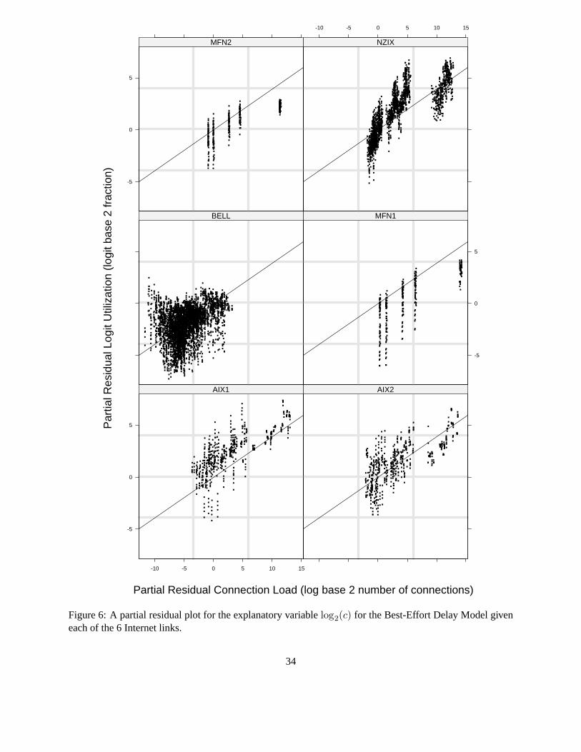
.....
.....
..
...
..
...
..
..
.
....
.
...
..
..
..
.
..
..
.
..
..
.
.
..
..
.
..
..
.
..
..
.
..
..
.
..
..
.
..
..
.
..
..
.
..
..
.
..
..
.
..
..
...
..
.
..
..
.
..
..
.
..
..
.
..
..
.....
..
...
..
...
..
...
.
..
..
.....
..
...
..
...
..
...
.
..
..
.....
.....
.....
.....
...
..
...
..
..
.
..
..
.
..
..
.
..
..
...
..
.
..
..
.
..
..
.
..
.
..
..
.
..
..
.....
.....
.....
.....
.....
.....
..
...
..
...
..
...
.
..
..
.....
.....
.....
.....
.....
.....
...
..
..
...
..
...
..
...
...
..
..
...
..
...
...
..
...
..
.....
..
...
.....
.....
...
..
.....
.
....
..
...
..
...
.
..
..
..
...
..
...
..
...
.
..
..
.
..
..
.
..
..
.
..
..
.
..
..
.
..
..
.
..
..
...
..
...
..
..
.
..
..
.
..
..
...
..... ..... .....
.....
.....
..... .....
..
....
....
.....
.....
.....
.....
.....
.....
-5
0
5
AIX1
-10 -5 0 5 10 15
.....
..
...
..
...
..
...
..
...
.....
.....
.....
..
...
..
...
.
..
..
.
..
..
.
..
..
.
..
..
.
..
..
..
...
.
....
.
....
.
....
.
...
.
...
..
..
...
..
...
..
...
.
..
..
.....
..
...
..
...
.
....
.
..
..
.
..
..
.
..
..
.
..
..
.
..
..
.
..
..
...
..
..
...
..
...
..
...
...
..
..
...
..
...
.
..
..
.
..
..
.
..
..
.
..
..
.
..
..
.
..
..
.
..
..
.
..
..
.....
...
..
...
..
...
..
.....
.....
.....
...
..
...
..
..
...
.....
.....
...
..
...
..
...
..
.....
...
..
...
..
..
.
..
..
.
..
...
..
...
..
...
..
..
...
..
...
....
. ....
. ....
. ....
. ..... .
..
..
...
..
...
..
...
..
...
..
...
..
.
..
..
.
..
..
.
....
.
....
.....
.....
...
..
...
..
..
...
...
..
..
...
..
...
...
..
...
..
.
....
.
....
...
.....
..
.....
...
..
..
...
..
...
...
..
..
.
..
...
..
..
.
..
..
...
..
...
..
.
..
AIX2
.... .
...
. .
...
. .
.
... .
.
... .
...
..........
.....
..
..
...
...
....... ........
.....
..
.
... .
.... ..... ..... ....
. ....
. ....
. ....
. ....
. ....
. .
.
.... ..... ........
..
...
..
...
..
..... ..... ..... ..... .
....
.....
.....
.....
..... ..... ...
.. ...
.....
.....
.. .
....
.....
.....
..... .....
........
.....
.....
.....
...
.......
...............
..
.....
..... ..... ..... ..... .....
..... ..... ..... ......
.......
....... ...
.....
.......
..........
..
...
..
...
.....
..... ..... ..... ..... .
....
.....
.....
.....
......
....
.....
.....
.....
..... ...
..
..... ..... ..... .....
...
..
...
..
...
..
.....
.....
...
..
.....
.....
..... ........
..
.....
.....
...
.....
..
..... ..... ..... ..... .....
.....
.....
..... .....
......
....
.....
..... ..... ..... .
....
.....
.....
.....
..... ...
..
.....
..... ..... ......
....
...
..
...
..
...
..
...
.. .....
.
....
.
....
...
....... .
....
...
..
.....
.....
......
....
.....
.....
.....
...
..
.....
.....
.....
.....
......
........................
...
..
.....
..... ..... ..... .
....
.....
...
..
...
...
..
..
..... ..... ..... ..... .....
...
..
...
..
...
..
...
..
.....
.
..
..
...
..
...
..
...
..
.....
...
.....
..
.....
.....
..... .
.... ..... .....
.....
...
..
...
..
...
..
...
..
...
..
...
..
.....
...
..
...
..
...
..
...
..
...
..
.....
..... ..... ..... .
..
..
.
....
...
..
...
..
...
..
.
..
..
.....
.....
.....
..... .....
.....
...
..
...
..
...
..
.
.
...
.
....
.....
.....
.....
.....
...
..
...
..
...
..
...
..
.....
.....
.....
.....
.....
.....
...
..
.....
.....
..... ..... .....
.....
.....
...
.....
..
...
..
.....
.....
...
..
...
..
.....
.....
.....
..... ...
..
...
..
...
..
...
..
.....
...
..
...
..
.....
.....
........
..
.....
.....
.....
.....
...
..
.....
.....
.....
...
...
....
...
..
...
..
...
..
...
..
...
..
...
..
...
..
...
..
...
...
....
.
..
..
.
.......
..
...
..
..... ..... ..... ..... ..... .
..
..
...
..
...
..
.
..
..
.
..
..
...
..
...
..
.....
.....
.....
.
..
..
...
..
...
..
...
..
...
..
.
..
..
...
..
...
..
.
..
..
.
..
..
...
..
...
..
...
..
...
..
...
..
.
....
.
....
.
..
.....
.....
..
.....
.....
.....
..... .....
.....
.....
.....
.....
..... .
..
..
...
..
.....
...
..
...
..
.....
.....
.....
.....
...
..
.
....
.
..
..
.
..
..
...
..
.....
..... ..... .....
.....
.....
...
..
...
..
...
..
...
..
.
....
...
..
.....
.....
.....
.....
...
..
...
..
...
..
...
..
...
.....
..
.....
.....
.....
.....
...
..
...
..
...
..
...
..
...
..
...
..
...
..
.
..
..
...
..
...
..
...
..
...
..
.....
.....
.....
...
..
.....
.....
.....
...
..
...
..
...
..
...
..
...
..
..... .....
.....
.....
.....
..... .
..
.....
..
...
..
...
..
...
..
.
....
.
....
.....
.....
.....
...
..
...
..
...
..
...
..
...
...
....
...
.....
.....
.....
..
...
..
...
..
...
..
.....
.....
.....
.....
.....
.....
.....
.....
...
..
...
..
...
..
...
..
.....
...
..
...
..
...
..
...
..
.....
.....
.....
...
..
...
.....
..
...
..
...
..
...
..
........
.....
..
.....
.....
.....
..... .....
.....
...
..
...
...
....
...
..
.....
.....
...
...
.......
.....
..
.....
.....
.....
.....
.....
.....
.....
.....
.....
.....
.....
...
.....
..
.....
.....
.....
..... .
....
...
..
...
..
.....
.....
.....
.....
.....
.....
.......
... .....
.....
.....
...
..
...
..
...
..
...
..
...
..
.....
.
..
..
.
..
..
.
.
.
..
.
.
.
..
.
..
..
...
..
...
..
...
..
.....
...
..
...
.....
.....
.....
..
.....
...
..
...
..
...
..
...
..
...
..
.....
...
..
...
..
...
..
...
.. .....
...
..
...
..
...
..
.....
...
..
...
..
...
..
.....
...
.. ...
..
.....
...
..
.....
...
..
...
..
.....
.....
...
..
...
.. ....
. .....
.....
.....
.....
.....
.....
.....
.....
.....
...
..
...
..
...
..
..
.
..
...
..
.....
.....
.....
.....
..... .
....
.....
...
..
.....
...
.. ...
.....
..
.....
...
..
...
..
...
..
...
..
...
..
...
..
...
..
...
..
.....
.....
...
..
...
..
.....
...
..
...
..
...
..
...
.......
...
..
...
..
...
..
..... .
....
...
...
....
.....
.
..
..
...
..
...
..
...
..
...
..
...
..
.
....
.....
...
...
....
...
..
...
..
...
..
...
..
...
..
...
..
...
..
...
..
...
..
...
..
.....
...
..
...
..
...
..
...
..
...
..
...
..
.....
.....
.....
.....
...
..
...
..
...
..
.....
...
..
...
..
...
..
...
..
...
..
...
..
.....
.....
.....
.....
.....
...
..
...
..
...
..
...
..
.....
...
..
.....
.....
.....
...
.. .....
.....
.....
.....
.....
...
..
.....
...
..
...
..
...
..
...
..
...
..
.....
.....
.....
...
..
..
.
..
...
..
...
..
...
..
...
..
...
..
.....
...
..
.....
.....
.....
.....
...
..
...
...
....
.....
.....
.....
.....
.
....
...
..
...
..
...
..
...
..
...
..
...
..
...
..
...
..
...
...
.... .....
...
..
...
..
.....
...
..
...
..
...
..
...
..
...
..
.....
...
..
...
..
...
..
...
.......
.....
...
..
...
..
...
..
...
..
...
..
...
..
.....
..... .
....
...
..
.....
.....
...
..
...
..
...
..
...
..
...
..
...
..
.....
...
..
...
..
...
..
...
..
...
..
...
..
..
.
..
...
..
..
.
..
...
..
...
..
...
..
...
..
...
..
...
..
...
..
...
..
...
..
...
..
.....
.....
.....
.....
..... .
....
...
..
...
..
...
..
...
..
.....
...
..
...
..
...
..
...
..
...
..
...
..
...
..
...
..
...
..
...
..
...
..
..
.
..
..
.
..
...
..
...
..
...
..
...
..
...
..
...
.. ...
..
...
..
.
..
..
.
..
..
.
..
..
...
..
...
..
...
..
...
..
..
.
..
.
....
...
..
...
..
...
..
...
..
...
..
...
..
...
..
...
..
...
..
...
..
...
..
...
..
.....
.....
.....
...
..
...
..
...
..
...
...
....
...
..
...
..
...
..
...
..
..... ..... ..... .....
.....
...
..
...
..
...
..
...
..
...
....
... ........
..
.....
.....
.....
.....
.....
...
..
...
..
...
..
.....
.....
...
..
...
..
...
..
...
..
...
..
...
..
...
....
... .
....
.....
.....
.....
...
..
.
..
..
...
..
...
..
...
..
.....
.....
.....
...
..
...
..
.....
...
..
.....
.....
.....
...
..
...
..
...
..
...
..
...
..
...
..
...
..
.
..
..
.
..
..
.
..
..
..
... .....
...
..
...
..
...
..
.....
...
...
....
...
..
...
..
.
....
.
..
..
...
..
...
..
...
.. .....
...
.....
..
...
..
...
..
...
..
...
..
...
..
...
..
...
..
...
.....
.....
..
.....
...
.......
...
..
...
..
...
..
...
..
...
..
...
..
...
..
...
..
...
..
...
..
...
..
...
..
...
..
...
...
....
...
..
...
..
...
..
...
..
.
....
...
..
...
..
...
..
...
..
...
..
..
.
..
...
..
...
..
..
.
..
...
..
...
..
...
..
...
..
...
..
...
..
...
..
...
..
...
..
...
..
BELL
...
..
..
...
..
...
..
...
.
..
..
..
...
.
..
..
.
..
..
.
..
..
.
..
..
...
..
..
.
..
..
.
..
..
...
.
..
..
..
.
..
.
..
..
.
..
..
.
..
..
.
..
..
...
..
...
..
..
.
..
..
.
..
.
..
..
...
..
..
...
..
...
..
...
..
...
.
..
..
.
..
..
.
..
..
.
..
..
.
..
..
.
..
..
.
..
..
.
..
..
.
..
..
.
..
..
...
..
..
...
..
...
..
...
.
..
..
.
..
..
.
..
..
.
..
..
.
..
..
.
..
..
...
..
..
...
..
...
..
...
..
...
...
..
...
..
..
...
..
...
..
...
-5
0
5
MFN1
..
.
..
..
.
..
..
.
..
.
..
..
.
..
..
.....
.....
.....
...
..
..
...
.....
.....
.....
.....
..
...
...
..
..
...
..
...
..
...
.
....
...
..
...
..
..
.
..
..
.
..
.
..
..
...
..
...
..
..
...
..
...
.
..
..
...
..
...
..
.....
...
..
..
...
.....
.....
.....
.....
...
..
.....
.....
.....
...
..
..
...
...
..
...
..
..
...
..
...
.
....
...
..
...
..
.....
...
..
...
..
...
..
...
..
..
...
..
...
...
..
-5
0
5
MFN2
..
.
..
...
..
...
..
...
..
...
..
...
..
...
..
...
..
...
..
..
.
..
..
..
.
...
..
...
..
..
.
..
..
.
..
.
..
..
.
..
..
.
..
..
.
..
..
.
..
..
...
..
...
..
...
..
...
..
...
..
..
.
..
..
.
..
..
.
..
...
..
...
..
..
...
...
..
...
..
...
..
...
..
....
.
...
..
...
..
...
..
...
..
...
..
...
..
...
..
...
..
..
.
..
..
.
..
..
.
..
...
..
...
..
..
.
..
...
..
..
..
.
..
..
.
..
.
..
...
..
...
..
...
..
..
.
..
..
.
..
..
.
..
...
..
...
..
...
..
...
..
..
.
..
..
..
.
..
..
.
...
..
..
.
..
..
.
..
..
.
..
..
.
..
..
.
..
..
.
..
..
.
..
...
..
..
.
..
..
.
..
..
.
..
..
.
..
...
..
...
..
...
..
...
..
..
.
..
...
..
...
..
...
..
...
..
...
..
...
..
...
..
...
..
...
..
...
..
..
...
..
.
..
..
.
..
..
.
..
..
.
..
...
..
...
..
...
..
...
..
...
..
...
..
...
..
..
.
..
...
..
...
..
...
..
...
..
...
..
...
..
...
..
.....
.
....
.
....
.
....
.
....
...
..
..
.
..
...
..
...
..
....
.
.
..
..
.
..
..
.
..
..
.
..
..
.
..
..
.
..
..
.
..
..
..
.
..
..
.
..
.
..
..
.....
.
....
...
..
...
..
...
..
...
..
..
.
..
..
.
..
..
.
..
...
..
..
..
.
...
..
..
.
..
..
.
..
..
.
..
...
..
...
..
..
.
..
..
.
..
..
.
..
...
..
...
..
...
..
...
..
..
.
..
..
.
..
...
..
...
..
..
.
..
..
.
..
..
.
..
...
..
...
..
...
..
..
.
..
...
..
...
..
...
..
...
..
..
.
..
...
..
..
.
..
..
.
..
..
.
..
...
..
..
.
..
..
.
..
..
.
..
..
.
..
..
.
..
....
.
...
..
..
.
..
..
.
..
...
..
..
.
..
..
.
..
...
..
...
..
.....
...
..
..
.
..
...
..
...
..
...
..
...
..
..
.
..
...
..
...
..
...
..
.....
...
..
...
..
..
.
..
...
..
..
.
..
..
.
..
..
.
..
..
.
..
...
..
..
..
.
..
.
..
..
.
..
..
.
..
..
.
..
...
..
..
.
..
..
.
..
..
.
..
..
.
..
..
.
..
..
.
..
..
.
..
..
.
..
..
.
..
...
..
..
.
..
..
.
..
..
.
..
..
.
..
...
..
..
..
.
..
..
.
..
.
..
..
.
..
..
.
..
..
.
..
..
.
..
..
.
..
..
.
..
..
...
..
..
.
..
.
..
...
..
...
..
..
.
..
..
.
..
..
.
..
..
.
..
..
.
..
..
.
..
..
.
..
..
.
..
..
.
..
...
..
..
..
.
..
.
..
..
.
..
..
..
.
...
..
...
..
..
.
..
..
.
..
..
.
..
...
..
..
.
..
..
.
..
..
.
..
..
.
..
...
..
...
..
..
.
..
..
.
..
...
..
...
..
...
..
..
.
..
..
.
..
..
.
..
...
..
...
..
...
..
..
.
..
...
..
...
..
...
..
...
..
...
..
.....
.....
..
.
..
..
.
..
...
..
...
..
..
.
..
...
..
...
..
.....
...
..
.....
..
.
..
..
.
..
...
..
...
..
..
.
..
...
..
..
.
..
...
..
...
..
...
..
..
.
..
..
.
..
..
.
..
...
..
..
.
..
..
.
..
..
.
..
..
.
..
...
..
...
..
...
..
..
.
..
..
.
..
..
.
..
...
..
..
.
..
.
..
..
.
..
..
.
..
..
.
..
..
...
..
..
.
..
..
.
..
..
.
..
...
..
...
..
..
.
..
..
.
..
..
.
..
..
.
..
..
.
..
..
.
..
..
.
..
..
.
..
..
.
..
..
..
.
..
..
.
..
.
..
..
.
..
..
.
..
...
..
..
.
..
..
.
..
..
.
..
...
..
...
..
..
.
..
..
.
..
..
.
..
..
.
..
..
.
..
..
.
..
..
.
..
..
.
..
.
..
..
...
..
..
.
..
..
.
..
..
.
..
..
.
..
...
..
..
.
..
..
.
..
..
.
..
...
..
..
.
..
..
.
..
...
..
...
..
..
.
..
..
...
...
..
...
..
..
.
..
..
.
..
.
....
.
....
...
..
...
..
..
...
..
.
..
..
.
..
...
..
...
..
..
.
..
...
..
..
.
..
..
.
..
...
..
...
..
...
..
...
..
..
.
..
..
.
..
..
.
..
...
..
..
.
..
..
.
..
..
.
..
.
..
..
..
...
..
.
..
..
.
..
..
.
..
..
.
..
NZIX
-10 -5 0 5 10 15
Partial Residual Connection Load (log base 2 number of connections)
Par
tial R
esid
ual L
ogit
Util
izat
ion
(logi
t bas
e 2
frac
tion)
Figure 6: A partial residual plot for the explanatory variable log2(c) for the Best-Effort Delay Model giveneach of the 6 Internet links.
34

.... . .
AIX1
AIX2
BELL
MFN1
MFN2
NZIX
-0.4 -0.2 0.0 0.2 0.4 0.6 0.8
Median Residual Logit Utilization (logit base 2 fraction)
Figure 7: Dotplot of link median residuals for the Best-Effort Delay Model.
Let t15(p) be the quantile of probability p of a t distribution with 15 degrees of freedom. Then the lowerlimit of a 100(1 − p)% tolerance interval for ` is
ˆ(p) = ˆ− mδ(ψ)t15(p)/0.691.
For p = 0.05, t15(p) = 1.75, so the lower 95% limit is
ˆ(0.05) = ˆ− 2.53mδ(ψ).
The lower 95% limit on the utilization scale is
u(0.05) =2
ˆ(0.05)
1 + 2ˆ(0.05).
This process is illustrated in Figure 8. For the figure, γb was taken to be 214 bits/sec/connection. On eachpanel, the values of τ and ω are fixed to the values shown in the strip labels at the tops of the panels, and uand u(0.05) are both graphed against log2(δ) for δ varying from 0.001 sec to 0.1 sec.
11.9 Other Work on Bandwidth Estimation and Comparison with the Results Here
Bandwidth estimation has received much attention in the literature. The work focuses on queueing becausethe issue driving estimation is queueing. Some work is fundamentally empirical in nature in that it uses livestreams as inputs to queueing simulations or synthetic streams from models that have been built with livestreams, although theory can be invoked as well. Other work is fundamentally theoretical in nature in thatthe goal is to derive mathematically properties of queues, although live data are sometimes used to providevalues of parameters so that numerical results can be calculated. Most of this work uses derivations of thedelay exceedance probability as a function of an input source to derive the required bandwidth for a givenQoS requirement. The delay exceedance probability is equivalent to the our delay probability, where thebuffer size is related to the delay by a simple multiplication of the link bandwidth. Since exact calculationsof the delay probability are only feasible in special cases, these methods seek an approximate analysis, forexample, using asymptotic methods, stochastic bounds, or in some cases, simulations. There has been byfar much more theoretical work than empirical.
35

0.0
0.2
0.4
0.6
0.8
1.0
1 mbps0.1%
0.0 0.5 1.0 1.5 2.0
10 mbps0.1%
100 mbps0.1%
0.0 0.5 1.0 1.5 2.0
500 mbps0.1%
1 mbps1%
10 mbps1%
100 mbps1%
0.0
0.2
0.4
0.6
0.8
1.0
500 mbps1%
0.0
0.2
0.4
0.6
0.8
1.0
1 mbps5%
10 mbps5%
0.0 0.5 1.0 1.5 2.0
100 mbps5%
500 mbps5%
0.0 0.5 1.0 1.5 2.0
Log Delay (log base 10 ms)
Util
izat
ion
(fra
ctio
n)
Figure 8: The QoS utilization from the Best-Effort Delay Model is graphed against log delay given thebit rate and the delay probability. The bit connection rate γb is taken to be 214 bits/sec/connection. Theupper curve on each panel estimates the expected values and the lower curve is the minimum values of 95%tolerance intervals.
36
The attention to the statistical properties of the traffic stream, which have an immense impact on the queue-ing, receives attention to varying degrees. Those who carry out empirical studies with live streams do soas a guarantee of recreating the properties. Those who carry out studies with synthetic traffic from modelsmust argue for the validity of the models. Much of the theoretical work takes the form of assuming certainstream properties and then, deriving the consequences, so the problem is solved for any traffic that mighthave these properties. Sometime, though, the problem is minimized by deriving asymptotic results undergeneral conditions.
11.9.1 Empirical Study
Our study here falls in the empirical category but with substantial guidance from theory. To estimate ex-ceedance probabilities, we run simulations of an infinite buffer, FIFO queue with fixed utilization using livepacket streams or synthetic streams from the FSD model as the input source.
The tradition for using live Internet streams in a queueing simulation began early in the study of Internettraffic. In a very important study it was shown that long-range dependent traffic results in much greaterqueue-length distributions (Erramilli, Narayan, and Willinger 1996) than Poisson traffic. This was an im-portant result because it showed that the long-range dependence of the traffic would have a large impact onInternet engineering. In other studies, queueing simulations of both live and altered live traffic are used tostudy the effect of dependence properties and multiplexing on performance using the average queue lengthas the performance metric (Erramilli, Narayan, Neidbardt, and Saniee 2000; Cao, Cleveland, Lin, and Sun2001; Erramilli, Narayan, Neidbardt, and Saniee 2000).
In (Mandjes and Boots 2004), queueing simulations of multiplexed on-off sources are used to study theinfluence of on and off time distributions on the shape of the loss curve and on performance. To improve theaccuracy of the delay probabilities based on simulations, techniques such as importance sampling are alsoconsidered (Boots and Mandjes 2001).
One study (Fraleigh, Tobagi, and Diot 2003) first uses live streams, Internet backbone traffic, to validate atraffic model: an extension of Fractional Brownian Motion (FBM), a two-scale FBM process. They do notmodel the packet process but rather bit rates as a continuous function. Then they derive approximations ofthe delay exceedance probability from the model, which serves as the basis for their bandwidth estimation.Parameters in the two-scale FBM model that appear in the formula are related to the bitrate τ using thedata. This is similar to our process here where we relate the stream coefficients to c and τ . They alsoused queueing simulations to determine delay exceedance probabilities as a method of validation. We willcompare their results and ours at the end of this section.
11.9.2 Mathematical Theory: Effective Bandwidth
A very large number of publications have been written in an area of bandwidth estimation that is referredto as “effective bandwidth”. The effective bandwidth of an input source provides a measure of its resourceusage for a given QoS requirement, which should lie somewhere between the mean rate and peak rate.Let A(t) be the total workload (e.g., bytes) generated by a source in the interval [0, t], the mathematicaldefinition of the effective bandwidth of the source (Kelly 1996) is
α(s, t) =1
stlog E[esA(t)] 0 < s, t <∞, (8)
37

for some space parameter s and time parameter t. For the purpose of bandwidth estimation, the appropriatechoice of parameters depends on the traffic characteristics of the source, the QoS requirements, as well asthe properties of the traffic with which the source is multiplexed. In the following we shall discuss theeffective bandwidth approach to bandwidth estimation based on approximating the delay probability in theasymptotic regime of many sources.
Consider the delay exceedance probability for a First In First Out (FIFO) queue on a link with constant bitrate. In the asymptotic regime of many sources, we are concerned with how the delay probability decaysas the size of the system increases. Suppose there are n sources and the traffic generated by the n sourcesare identical, independent and stationary. The number of sources, n, grows large and at the same timethe resources such as the link bandwidth β and buffer sizes scale proportionally so that the delay δ staysconstant. Let β = nβ0 for some β0, and let Qn be the queueing delay. Under very general conditions, itcan be shown that (Botvich and Duffield 1995; Courcoubetis and Weber 1996; Simonian and Guibert 1995;Likhanov and Mazumdar 1998; Mandjes and Kim 2001)
limn→∞
−n−1 log P(Qn > δ) = I(δ, β0), (9)
whereI(δ, β0) = inf
t>0sup
s(sβ0(δ + t) − stα(s, t)) , (10)
and is sometimes referred to as the loss curve in the literature. Let (s∗, t∗) be an extremizing pair in Equa-tion (10), then α(s∗, t∗) is the effective bandwidth for the single source as defined in Equation (8), andnα(s∗, t∗) is the effective bandwidth for the n sources. For a QoS requirement of a delay δ and a delayprobability w, approximating the delay probability P(Qn > δ) using exp(−nI(δ, β0)) (Equation 9), thebandwidth required for the n sources can be found by solving the following equation for β
s∗β(δ + t∗) − s∗t∗nα(s∗, t∗) = − logw. (11)
This gives
β =s∗t∗
s∗(δ + t∗)nα(s∗, t∗) −
logw
s∗(δ + t∗), (12)
which is the effective bandwidth solution to the bandwidth estimation problem. If the delay δ → ∞, thenthe extremizing value of t∗ approaches to ∞, and the bandwidth in Equation (12) reduces to
n limt∗→∞
α(s∗, t∗),
and we recover the classical effective bandwidth definition of a single source limt∗→∞ α(s∗, t∗) for thelarge buffer asymptotic model (Elwalid and Mitra 1993; Guerin, Ahmadi, and Naghshineh 1991; Kesidis,Walrand, and Chang 1993; Chang and Thomas 1995). If the delay δ → 0, then the extremizing pair t∗ → 0and s∗t∗ → s for some s, the bandwidth in Equation (12) reduces to
n limt∗→∞
α(s/t∗, t∗) −logws
,
and we recover the effective bandwidth definition limt∗→∞ α(s/t∗, t∗) for the buffer-less model (Hui 1988).
As we can see, the effective bandwidth solution requires the evaluation of the loss curve I(δ, β0) (Equa-tion 10). However, explicit form of the loss curve is generally not available. One approach is to derive ap-proximations of the loss curve under buffer asymptotic models, i.e., large buffer asymptotic model (δ → ∞)
38

or buffer-less model (δ → 0), for some classes of input source arrivals. For example, if the source arrivalprocess is Markovian, then for some η > 0 and ν (Botvich and Duffield 1995)
limδ→∞
I(δ, β0) − ηδ = ν.
If the source arrival is Fractional Brownian Motion with Hurst parameter H , then for some ν > 0 (Duffield1996)
limδ→∞
I(δ, β0)/δ2−2H = ν.
For on-off fluid arrival process, it is shown that as δ → 0, for some constants η(β0) and ν(β0) (Mandjes andKim 2001),
I(δ, β0) ∼ η(β0) + ν(β0)√δ +O(δ),
and as δ → ∞, for some constant θ(β0) (Mandjes and Boots 2002),
I(δ, β0) ∼ θ(β0)v(δ),
where v(δ) = − log P(Residual On period > δ). However, it is found that bandwidth estimation based onbuffer asymptotic models suffer practical problems. For the large buffer asymptotic model, the estimatedbandwidth could be overly conservative or optimistic due to the fact that it does not take into account thestatistical multiplexing gain (Choudhury, Lucantoni, and Whitt 1994; Knightly and Shroff 1999). For thebuffer-less model, there is a significant utilization penalty in the estimated bandwidth (Knightly and Shroff1999) since results indicate that there is a significant gain even with a small buffer (Mandjes and Kim 2001).
Another approach proposed by (Courcoubetis, Siris, and Stamoulis 1999; Courcoubetis and Siris 2001) isto numerically evaluate the loss curve I(δ, β0). First, they evaluate the effective bandwidth function α(s, t)(Equation 8) empirically based on measurements of traffic byte counts in fixed size intervals, and thenthey obtain the loss curve (Equation 10) using numeric optimizing procedures with respect to the spaceparameter s and the time parameter t. As examples, they applied this approach to estimate bandwidth wherethe input source is a Bellcore Ethernet WAN streams or streams of incoming IP traffic over the University ofCrete’s wide area link. Their empirical approach is model free in the sense that it does not require a trafficmodel for the input source and all evaluations are based on traffic measurements. However, their approachis computational intensive, not only because the effective bandwidth function α(s, t) has to be evaluatedfor all time parameters t, but also because the minimization with respect to t is non-convex (unlike themaximization in the space parameter s) and thus difficult to perform numerically (Gibbens and Teh 1999;Kontovasilis, Wittevrongel, Bruneel, Houdt, and Blondia 2002).
In the effective bandwidth approach, one typically approximates the buffer exceedance probability based onits logarithmic asymptote. For example, in the asymptotic regime of many sources, using Equation (9), onecan approximate
P(Qn > δ) ≈ exp(−nI(δ, β0)). (13)
An improved approximation can be found by incorporating a pre-factor, i.e.
P(Qn > δ) ≈ K(n, δ, β0) exp(−nI(δ, β0)).
Using the Bahadur-Rao theorem, such approximation has been obtained for the delay exceedance probabilityin the infinite buffer case as well as the cell loss ratio in the finite buffer case that has the same logarithmicasymptote but a different pre-factor (Likhanov and Mazumdar 1998).
39

11.9.3 Theory: Other Service Disciplines
Some authors have investigated service disciplines other than FIFO such as general processor sharing(li Zhang, Towsley, and Kurose 1994) and priority queue (Berger and Whitt 1998). Although TCP is themost dominant protocol in today’s Internet, we do not consider the effect of the TCP feedback control mech-anism since the link we sought for estimating a bandwidth is not a bottleneck link. To account for the TCPfeedback control, other authors have studied characteristics of bandwidth sharing for elastic traffic and in-vestigated the bandwidth estimation problem for such traffic (de Veciana, Lee, and Konstantopoulos 2001;Fredj, Bonald, Proutiere, Regnie, and Roberts 2001). Again other authors have considered regulated inputtraffic such as those from a leaky bucket (Elwalid, Mitra, and Wentworth 1995; Presti, Zhang, Kurose, andTowsley 1999; Kesidis and Konstantopoulos 2000; Cheng-Shang Chang and Song 2001).
11.9.4 Theory: Direct Approximations of the Delay Probability
Besides approximating the delay exceedance probability using the effective bandwidth approach, some au-thors have considered direct approximations for some special classes of input traffic models. For example,for a Markov modulated fluid source, the delay probability can be more accurately expressed as a single ex-ponential with a prefactor K determined from the loss probability in a buffer-less multiplexer as estimatedby Chernoff’s theorem (Elwalid, Heyman, Lakshman, Mitra, and Weiss 1995). For an aggregate Markovmodulated fluid source, the delay probabilities can be approximated by a sum of exponentials (Shroff andSchwartz 1998). For a Gaussian process, a tight lower bound of the delay probability can be obtained usingmaximum-variance based approaches (Norros 1994; Knightly 1997; Kim and Shroff 1998; Fraleigh, Tobagi,and Diot 2003). These expressions can be used in place of Equation (13) to derive the required bandwidth fora QoS requirement. Readers are referred to (Knightly and Shroff 1999) for a nice overview and comparisonof these approaches as well as the aforementioned effective bandwidth approach for bandwidth estimation.
11.9.5 Theory: Queueing Distributions
We now discuss implications of our stream coefficient delay formula and Best-Effort Delay Formula andits relation to some previous work. The stream coefficient delay model in Equation 3 implies that for eachstream i,
w ≈ P(Qi > δ) ≈ exp
(
− log 2 · 2µiow
(
u
1 − u
)
−1
ow
δoδow
)
for stream coefficient µi and regression coefficients ow, oδ. This suggests the tail distribution of queueingdelay is Weibull with shape parameter oδo
−1w . The Weibull form is consistent with the FBM traffic model
(and also the two-scale FBM model), but there the shape parameter is 2 − 2H . Notice that oδo−1w from
our analysis is 0.52 for the real data and 0.42 for the synthetic data which is quite different from the shapeparameter computed from 2−2H = 0.18. If the bitrate per connection γb is a fixed constant, the Best-EffortDelay Formula in Equation 5 implies that for some constant o′
w ≈ P(Qi > δ) ≈ exp
(
− log 2 · 2o′
ow τoc+oτδ
owi
(
u
1 − u
)
−1
ow
δoδow
)
.
If oc + oτδ = ow and the traffic bitrate τi is a multiple of τ , i.e. τi = niτ , then the above approximation isconsistent with the effective bandwidth result with many sources asymptotics (Equation 9). In our empirical
40

analysis, we have found oτδ + oc and ow to be quite close with the ratio (oτδ + oc)o
−1w being 0.97 for real
data and 0.85 for synthetic data. One of the reasons that this ratio is not 1 is possibly due to the fact that(Equation 9) is an asymptotic formula.
11.9.6 Comparison of The Results Presented Here with Other Work
The work presented in this article has resulted in a simple formula for bandwidth estimation. At the sametime, validation has been extensive, permeating all areas of the work. Validation is carried out in two ways:empirically and theoretically.
The large number of papers in the area of effective bandwidth and other theoretical work cited above haveyielded much insight. The work has posited traffic stream models and investigated the resulting mathemat-ical properties. However, for best-effort Internet traffic, there has not been extensive study to determinewhether some posited model accurately describes the stream statistical properties. Nor has there been exten-sive empirical work in the form of extensive empirical queueing simulations to determine whether queueingresults for best-effort traffic fit the theory. Consequently, the simple Best-Effort Delay Formula, not readilyderivable without a hint of the final results, was not uncovered.
The interesting paper cited above using the two-scale FBM model surely took great pains to validate themodel (Fraleigh, Tobagi, and Diot 2003). One problem with this approach, modeling traffic bit flow as afluid rather than the packet process as it appears on the link, is that the Gaussian assumption does not takehold until the level of aggregation is quite high. Consequently, the FBM model is not a good approximationuntil the traffic rate is 50 megabits/sec and above. So their bandwidth estimation model is not a validated onebelow 50 megabits/sec. By contrast, our Best-Effort Delay Model is valid to as low as 1 megabit/sec. Butthe ensuing methods used in (Fraleigh, Tobagi, and Diot 2003) to find the QoS bandwidth require a series ofapproximations and a worst-case empirical method in the estimation of parameters. There appears to havebeen little checking of these approximations. The bandwidth results appear to us to be inaccurate, possiblyarising from some of the approximations. First, as the bit rate increases up to 1 gigabit/sec, the utilizationappears to stabilize at values less than 1, substantially so in some cases. As our theoretical discusses of rategains and multiplexing gains demonstrates, the utilization must increases to 1 as the bitrate increases. Thisis the case for our Best-Effort Delay Model. For example, the utilization for a delay of 10 ms, a probabilityof 0.01, and a bit rate of 1 gigabit/sec, is 90% from Figure 8 of (Fraleigh, Tobagi, and Diot 2003) but is98% for our model. In addition, the model in (Fraleigh, Tobagi, and Diot 2003) works simply with the bitrate rather than decomposing into the number of active connections times the bit rate per connection andusing two variables, as is done in the Best-Effort Delay Model here. As we have demonstrated, theoreticallyand empirically, the bit rate is not sufficient to account for the utilization since a fast network and one witha high traffic connection load must be distinguished.
11.10 Results and Discussion
11.10.1 Problem Formulation
Suppose the packet stream — packet arrival times and sizes — arriving for transmission on an Internet linkis best-effort traffic with bit rate τ bits/sec and number of simultaneous active connections, c. Suppose thelink input buffer is large enough that packet loss is negligible. Our goal is to estimate the quality-of-service(QoS) bandwidth β in bits/sec, or equivalently, the QoS utilization u = τ/β, that satisfies QoS criteria for
41

the packet queueing delay in the link input buffer. The criteria are a delay, δ sec, and the probability, ω, thatthe delay for a packet exceeds δ.
11.10.2 Other Work on the Problem
There is a wide literature on the bandwidth estimation problem. Much of it is theoretical — mathematicalresults that derive properties of queueing systems. A smaller literature is empirical in nature, based onsimulations with packet stream inputs from measurements on live links or from models for traffic. Theclassical Erlang Delay Formula provides a simple formula that can be used for estimation of traffic streamsthat in theory have Poisson arrivals and i.i.d. exponential sizes. Best-effort traffic is much more complex, itis nonlinear and long-range dependent, and there has been to date no simple, validated formula for it.
11.10.3 Principal Result: The Best-Effort Delay Model
The principal result of this paper is a statistical model that provides a simple, validated formula for theestimation of bandwidth for best-effort traffic in the same way that the Erlang Delay Formula does for thePoisson-exponential case. The model has been validated through extensive empirical study and throughconsistency with certain theoretical properties of queueing.
The model consists of the Best-Effort Delay Formula plus random variation:
logit2(u) = o+ oc log2(c) + oτδ log2(τδ) + oω(− log2(− log2(ω))) + ψ.
ψ is a random error variable with mean 0 and median absolute deviation mδ(ψ), which depends on δ; log2
is the log base 2; and logit2(u) = log2(u/(1 − u)). The distribution of 0.691ψ/mδ(ψ) is a t-distributionwith 15 degrees of freedom. Estimates of the coefficients of the model are
o = −8.933 oc = 0.420 oτδ = 0.444 oω = 0.893.
mδ(ψ) is modeled as a function of δ: log2(mδ(ψ)) is a linear function of log2(δ) plus random variation.The estimate of the intercept of the line is –0.481, the estimate of the linear coefficient of the line is 0.166,and the estimate of the standard error is 0.189. The bit rate τ is equal to cγb where γb is the connection bitrate in bits/sec/connection. So the Best-Effort Delay Formula can also be written as
logit2(u) = o+ (oc + oτδ) log2(c) + oτδ log2(γbδ) + oω(− log2(− log2(ω))).
In this form we see the action of the amount of multiplexing of connections as measured by c, and the end-to-end connection speed as measured by γb. An increase in either results in an increase in the utilization ofa link.
The Best-Effort Delay Model is used to estimate the bandwidth required to carry best-effort traffic given δ,ω, τ , and c. The QoS logit utilization is estimated by
ˆ= −8.933 + 0.420 log2(c) + .444 log2(τδ) + 0.893(− log2(− log2(ω))),
so the QoS utilization is estimated by
u =2
ˆ
1 + 2ˆ.
42

The corresponding estimated bandwidth is τ/u. For such an estimate there is a 50% chance of being toolarge and a 50% chance of being too small. We might however, use a more conservative estimate thatprovides a much smaller chance of too little bandwidth. Let
mδ(ψ) = 2−0.481+0.166 log2(δ)
be the estimate of m(δ). Let t15(p) be the lower 100p% percentage point of a t-distribution with 15 degreesof freedom, where p is small, say 0.05. Let
ˆ(p) = ˆ− m(δ)t15(p)/0.691
Then
u(p) =2
ˆ(p)
1 + 2ˆ(p),
is a conservative utilization estimate, the lower limit of a 100p% tolerance interval for the QoS utilization.The corresponding estimated bandwidth is τ/u(p).
11.10.4 Methods
The Best-Effort Delay Model was built, in part, from queueing theory. Certain predictor variables weresuggested by the Erlang Delay Formula. Theory prescribes certain behavior as τ , c, or γb increase, resultingin rate gains, multiplexing gains, or fast-forward invariance, and the model was constructed to reproduce thebehavior.
The Best-Effort Delay Model was built, in part, from results of queueing simulations with traffic streaminputs of two types, live and synthetic. The live streams are measurements of packet arrivals and sizes for349 intervals, 90 sec or 5 min in duration, from 6 Internet links. The synthetic streams are arrivals andsizes generated by recently developed FSD time series models for the arrivals and sizes of best-effort traffic.Each of the live streams was fitted by two FSD models, one for the inter-arrivals and one for the sizes, anda synthetic stream of 5 min was generated by the models. The generated inter-arrivals are independent ofthe generated sizes, which is what we found in the live data. The result is 349 synthetic streams that matchthe statistical properties collectively of the live streams. For each live or synthetic stream, we carried out25 runs, each with a number of simulations. For each run we picked a delay δ and a delay probability ω;simulations were carried out to find the QoS bandwidth β, the bandwidth that results in delay probabilityω for δ. This also yields a QoS utilization u = τ/β. We used 5 delays — 0.001 sec, 0.005 sec, 0.010sec, 0.050 sec, 0.100 sec — and 5 delay probabilities — 0.001, 0.005, 0.01, 0.02, and 0.05 — employingall 25 combinations of the two delay criteria. The queueing simulation results in delay data: values of fivevariables — QoS utilization u, delay δ, delay probability ω, the mean number of active connections of thetraffic c, and the traffic bit rate τ . The delay data were used in the model building.
11.10.5 Validity and Applicability
Extensive data exploration with visualization tools, some shown here, demonstrate that the Best-Effort DelayModel fits the simulation delay data. This, of course, is necessary for the model to be valid. In addition,validity is supported by the model reproducing the theoretical queueing properties as just discussed.
43

The validity of the Best-Effort Delay Model depends on the validity of the traffic streams used as inputsto the queueing simulation; that is, the packet streams must reproduce the statistical properties of best-effort streams. Of course, the live streams of the study do so because they are best-effort traffic. Extensivevalidation has shown that the FSD models, used to generate the packet streams here, provide excellent fitsto best-effort packet streams when c is above about 64 connections, which for a link where γb is about 214
bits/sec/connection means τ is above about 1 megabit/sec. For this reason, only traffic streams with τ greaterthan this rate are used in the study, and the Best-Effort Delay Model is valid above this rate.
The results are only valid for links with a large enough buffer that the packet loss is negligible. We haveused open-loop study, which does not provide for the TCP feedback that occurs when loss is significant.This restriction also holds for the other work on bandwidth estimation cited here.
There is also a practical restriction on applicability. We have taken the range of our study to include trafficbit rates as low as about 1 megabit/sec. We have done this simply because we can do so and achieve validresults. But even for the least stringent of our delay criteria, δ = 0.1 sec delay and ω = 0.05 delay probability,the utilizations are low for rates in the range of 1 megabit/sec to 5 megabits/sec. This might well be judgedto be too small a utilization to be practical; if so, it might mean that the what must be sacrificed is thenegligible packet loss, which means that a QoS study at the very low traffic bit rates needs to take accountof TCP feedback.
One outcome of the dependence of the bandwidth estimation on the traffic statistics is that our solution forbest-effort traffic would not apply to other forms of Internet traffic that do not share the best-effort statisticalproperties. One example is voice traffic.
Finally, the Best-Effort Delay Model provides an estimation of bandwidth in isolation without consideringother network factors. A major factor in network design is link failures. Redundancy needs to be built intothe system. So an estimate of bandwidth from the model for a link based on the normal link traffic may bereduced to provide the redundancy. But the model still plays a role because the bandwidth must be chosenbased on link traffic, but now the traffic in the event of a failure elsewhere. Bibliography Becker, R. A., W. S. Cleveland, and M. J. Shyu (1996). The Design and Control of Trellis Display. Journalof Computational and Statistical Graphics 5, 123–155.
Berger, A. W. and W. Whitt (1998, August). Effective bandwidths with priorities. IEEE/ACM Transactionson Networking 6(4), 447–460.
Boots, N. and M. Mandjes (2001). Fast simulation of a queue fed by a superposition of many heavy-tailedsources. Probability in the Engineering and Informational Sciences 16, 205–232.
Botvich, D. D. and N. G. Duffield (1995). Large deviations, the shape of the loss curve, and economies ofscale in large multiplexers. Queueing Systems 20, 293–320.
Cao, J., W. S. Cleveland, D. Lin, and D. X. Sun (2001). On the Nonstationarity of Internet Traffic. ACMSIGMETRICS 29(1), 102–112.
Cao, J., W. S. Cleveland, D. Lin, and D. X. Sun (2002). Internet Traffic Tends Toward Poisson andIndependent as the Load Increases. In C. Holmes, D. Denison, M. Hansen, B. Yu, and B. Mallick (Eds.),Nonlinear Estimation and Classification, pp. 83–109. New York: Springer.
44

Cao, J., W. S. Cleveland, and D. X. Sun (2004). Fractional Sum-Difference Models for Open-Loop Gen-eration of Internet Packet Traffic. Technical report, Bell Labs, stat.bell-labs.com.
Cao, J. and K. Ramanan (2002). A Poisson Limit for Buffer Overflow Probabilities. In IEEE INFOCOMM,Volume 2, pp. 994 – 1003.
Chang, C.-S. and J. Thomas (1995). Effective bandwidth in high speed digital networks. IEEE Journal onSelected Areas in Communications 13, 1091–1100.
Cheng-Shang Chang, Y.-m. C. and W. T. Song (2001). On the performance of multiplexing independentregulated inputs. In Proc. ACM Sigmetrics 2001/Performance 2001, pp. 184–193.
Choudhury, G. L., D. M. Lucantoni, and W. Whitt (1994). On the effectiveness of effective bandwidths foradmission control in atm networks. In Proceedings of the 14th International Teletraffic Congress (ITC-14),North Holland, pp. 411–420. Elsevier Science B. V.
Claffy, K., H.-W. Braun, and G. Polyzos (1995). A Parameterizable Methodology for Internet Traffic FlowProfiling. IEEE Journal on Selected Areas in Communications 13, 1481–1494.
Cooper, R. B. (1972). Queueing Theory. New York: Macmillan.
Courcoubetis, C. and V. A. Siris (2001). Procedures and tools for analysis of network traffic measurements.Technical report.
Courcoubetis, C., V. A. Siris, and G. D. Stamoulis (1999). Application of the many sources asymptoticand effective bandwidths to traffic engineering. Telecommunication Systems 12, 167–191.
Courcoubetis, C. and R. Weber (1996). Buffer overflow asymptotics for a buffer handling many trafficsources. Journal of Applied Probability 33, 886–903.
de Veciana, G., T.-J. Lee, and T. Konstantopoulos (2001, February). Stability and performance analysis ofnetworks supporting elastic services. IEEE/ACM Transactions on Networking 9(1), 2–14.
Duffield, N., A. Feldmann, J. Friedmann, A. Greenberg, R. Greer, T. Johnson, C. Kalmanek,B.Krishnamurthy, D. Lavelle, P. Mishra, K. Ramakrishnan, J. Rexford, F. True, , and J. van der Merwe(2000). Measurement and Analysis of IP Network Usage and Behavior. IEEE Communications MagazineMay, 82–86.
Duffield, N. G. (1996). Economies of scale in queues with sources having power-law large deviationsscalings. Journal of Applied Probability 33, 840–857.
Elwalid, A., D. Heyman, T. V. Lakshman, D. Mitra, and A. Weiss (1995, Aug). Fundamental bounds andapproximations for atm multiplexers with applications to video teleconferencing. IEEE Journal of SelectedAreas in Communications 13(6), 1004–1016.
Elwalid, A. and D. Mitra (1993). Effective bandwidth of general markovian traffic sources and admissioncontrol of high speed networks. IEEE/ACM Transactions on Networking 1, 329–343.
Elwalid, A., D. Mitra, and R. H. Wentworth (1995). A new approach for allocating buffers and bandwidthto heterogeneous regulated traffic in an atm node. IEEE Journal of Selected Areas in Communications13(6), 1115–1127.
Erramilli, A., O. Narayan, A. Neidbardt, and I. Saniee (2000). Performance Impacts of Multi-Scaling inWide Area TCP/IP traffic. In Proceedings of IEEE Infocom.
45

Erramilli, A., O. Narayan, and W. Willinger (1996). Experimental Queueing Analysis with Long-RangeDependent Packet Traffic. IEEE/ACM Transactions on Networking 4, 209–223.
Fraleigh, C., F. Tobagi, and C. Diot (2003). Provisioning ip backbone networks to support latency sensitivetraffic. In IEEE Infocom.
Fredj, S. B., T. Bonald, A. Proutiere, G. Regnie, and J. W. Roberts (2001, August). Statistical bandwidthsharing: A study of congestion at flow level. In SigComm’01, San Diego, California, USA, pp. 111–122.
Gao, J. and I. Rubin (2001). Multiplicative Multifractal Modeling of Long-Range-Dependent NetworkTraffic. International Journal of Communications Systems 14, 783–201.
Gibbens, R. J. and Y. C. Teh (1999, June). Critical time and space scales for statistical multiplexing. InProceedings of the 16th Internaltional Teletraffic Congress (TC 16), Edinburgh, UK, pp. 87–96.
Guerin, R., H. Ahmadi, and M. Naghshineh (1991, Sep). Equivalent capacity and its applications tobandwidth allocation in high-speed networks. IEEE Journal on Selected Areas in Communications 9(7),968–981.
Hosking, J. R. M. (1981). Fractional Differencing. Biometrika 68, 165–176.
http://pma.nlanr.net/PMA. Passive Measurement and Analysis Project at NLANR.
http://wand.cs.waikato.ac.nz/wand/wits/nzix/2/. NZIX-II Trace Data.
Hui, J. Y. (1988). Resource allocation for broadband networks. IEEE Journal Selected Areas in Commu-nications 6, 1598–1608.
Iyer, S., S. Bhattacharyya, N. Taft, N. McKeown, and C. Diot (2003). An approach to alleviate linkoverload as observed on an IP backbone. In IEEE Infocom, San Francisco.
Kelly, F. (1996). Notes on effective bandwidths. In S. Z. F.P. Kelly and I. Ziedins (Eds.), StochasticNetworks: Theory and Applications, Number 4 in Royal Statistical Society Lecture Notes Series, pp. 141–168. Oxford University Press.
Kesidis, G. and T. Konstantopoulos (2000, Jan). Worst-case performance of a buffer with independentshaped arrival processes. IEEE Communications Letters , 26–28.
Kesidis, G., J. Walrand, and C.-S. Chang (1993, August). Effective bandwidths for multiclass markovfluids and other atm sources. IEEE/ACM Transactions on Networking 1(3), 424–428.
Kim, H. and N. Shroff (1998, Oct). A central limit theorem based approach to analyze queue behavior inatm networks. IEEE/ACM Transactions on Networking 6, 659–671.
Knightly, E. (1997, June). Second moment resouce allocation in multi-service networks. In Proc. ACMSigmetrics ’97, Seattle, WA, pp. 181–191.
Knightly, E. W. and N. B. Shroff (1999, March/April). Admission control for statistical qos: Theory andpratice. IEEE Network 13(2), 20–29.
Konstantopoulos, T. and S.-J. Lin (1996, Dec.). High variability vs long-range dependence for networkperformance. In Proc. 35th. IEEE CDC, Kobe, pp. 1354–1359.
46

Kontovasilis, K., S. Wittevrongel, H. Bruneel, B. V. Houdt, and C. Blondia (2002). Performance oftelecommunication systems: Selected topics. In Communication Systems: the State of the Art. KluwerAcademic Publishers.
Leland, W., M. Taqqu, W. Willinger, and D. Wilson (1994). On the Self-Similar Nature of Ethernet Traffic.IEEE/ACM Transactions on Networking 2, 1–15.
li Zhang, Z., D. Towsley, and J. Kurose (1994). Statistical analysis of generalized processor sharingscheduling displine. In SigComm’94, London, England, UK, pp. 68–77.
Likhanov, N. and R. Mazumdar (1998). Cell loss asymptotics in buffers fed with a large number ofindependent stationary sources. In IEEE Infocom, pp. 339–346.
Mandjes, M. and N. Boots (2002). The shape of the loss curve, and the impact of long-range dependenceon network performance. Technical report.
Mandjes, M. and N. Boots (2004). The shape of the loss curve, and the impact of long-range dependenceon network performance. AEU International Journal on Electronics and Communications. to appear.
Mandjes, M. and J. H. Kim (2001). Large deviations for small buffers: an insensitivity result. QueuingSystems 37, 349–362.
Mosteller, F. and J. W. Tukey (1977). Data Analysis and Regression: A Second Course in Statistics.Reading, Massachusetts, U.S.A.: Addison-Wesley.
Norros, I. (1994). A Storage Model with Self-similar Input. Queueing Systems 16, 387–396.
Paxson, V. (1997). Automated Packet Trace Analysis of TCP Implementations. In ACM SIGCOMM, pp.167–179.
Paxson, V. and S. Floyd (1995). Wide-Area Traffic: The Failure of Poisson Modeling. IEEE/ACM Trans-actions on Networking 3, 226–244.
Presti, F. L., Z.-L. Zhang, J. Kurose, and D. Towsley (1999, August). Source time scale and optimalbuffer/bandwidth tradeoff for heterogeneous regulated traffic in a network node. IEEE/ACM Transactionson Networking 7(4), 490–501.
Ribeiro, V. J., R. H. Riedi, M. S. Crouse, and R. G. Baraniuk (1999). Simulation of NonGaussian Long-Range-Dependent Traffic Using Wavelets. ACM SIGMETRICS 27, 1–12.
Riedi, R. H., M. S. Crouse, V. J. Ribeiro, and R. G. Baraniuk (1999). A Multifractal Wavelet Model withApplication to Network Traffic. IEEE Transactions on Information Theory 45(3), 992–1019.
Shroff, N. B. and M. Schwartz (1998, August). Improved loss rate calculations at an atm multiplexer.IEEE/ACM Trans. on Networking 6(4), 411–422.
Simonian, A. and J. Guibert (1995). Large deviations approximation for fluid queues fed by a large numberof on/off sources. IEEE Journal of Selected Area in Communications 13, 1017–1027.
Stevens, W. R. (1994). TCP/IP Illustrated, Volume 1: The Protocols. Addison-Wesley.
47