internet appendix to are stocks really less volatile...
TRANSCRIPT
Internet Appendix to
Are Stocks Really Less Volatile in the Long Run?
by
Lubos Pastor
and
Robert F. Stambaugh
January 10, 2011
B1. Roadmap
This Appendix is organized as follows. A simple illustration demonstrating the effects of pa-
rameter uncertainty on long-horizon predictive variance is provided in Section B2. The Bayesian
empirical methodology for System 2 is presented in Section B3. Additional empirical evidence
that complements the evidence presented in the paper is reported in Section B4. That section first
presents the estimates of predictive regressions for both annual and quarterly data, followed by
various robustness results regarding the long-horizon predictive variance of stock returns.
B2. Parameter uncertainty: A simple illustration
In the paper, we compute Var(rT,T+k|DT ) and its components empirically, incorporating parameter
uncertainty via Bayesian posterior distributions. Here we use a simpler setting to illustrate the
effects of parameter uncertainty on multiperiod return variance. All the notation that is not defined
here is defined in Section 2 of the paper.
The elements of the parameter vector φ are viewed as random, given that they are unknown to
an investor. For the purpose of this illustration, we make several assumptions related to φ with the
objective of simplifying the variance ratio calculations in the presence of parameter uncertainty.
Our first assumption is that, given data DT , the elements of φ are distributed independently of
each other. We also make two assumptions about the deviations of the conditional mean from the
unconditional mean: given DT , µT − Er is uncorrelated with Er, and the quantity zT ≡ bT − Er
is fixed across φ. Next, let ρµb denote the true unconditional correlation between µT and bT ,
ρµb ≡ Corr(µT , bT |φ) (this correlation is “true” in that it depends on the true parameter values φ,
and it is “unconditional” in that it does not condition on DT ). If the observed predictors capture
µT perfectly, then ρµb = 1; otherwise ρµb < 1. We make the “homoskedasticity” assumption that
qT is constant across DT , which implies that
qT = (1 − ρ2µb)σ
2µ = (1 − ρ2
µb)R2σ2
r , (B1)
where σ2µ and σ2
r are the true unconditional variances of µt and rt+1, respectively (i.e., σ2µ ≡
Var(µt|φ) and σ2r ≡ Var(rt+1|φ)). The parameter vector is φ = [β,R2, ρuw, Er, σr, ρµb]. Finally,
we specify τ such that
Var(Er|DT ) = τE(σ2r |DT ) , (B2)
so that the uncertainty about the unconditional mean return Er is as large as the imprecision in a
sample mean computed over a sample of length 1/τ .
1
None of the above simplifying assumptions hold in the Bayesian empirical framework in the
paper; they are made for the purpose of this simple illustration only. Given these assumptions, we
are able to characterize the variance ratio in a parsimonious fashion that does not depend on the
unconditional variance of single-period returns.
The variance of the k-period return can be decomposed as follows:
Var(rT,T+k|DT ) = E Var(rT,T+k|φ, µT , DT )|DT + Var E(rT,T+k|φ, µT , DT )|DT
= E Var(rT,T+k|φ, µT )|DT + Var E(rT,T+k|φ, µT )|DT
= E
kσ2r(1 − R2)[1 + 2dρuwA(k) + d2B(k)]|DT
+Var
kEr +1 − βk
1 − β(µT − Er)|DT
= kE(σ2r |DT )E
(1 −R2)[1 + 2dρuwA(k) + d2B(k)]∣
∣
∣DT
+k2Var(Er|DT ) + Var
1 − βk
1 − β(µT −Er)|DT
= kE(σ2r |DT )E
(1 −R2)[1 + 2dρuwA(k) + d2B(k)]|DT
+k2τE(σ2r |DT ) + Var
1 − βk
1 − β(µT − Er)|DT
. (B3)
The next to last equality uses the property thatEr is uncorrelated with µT−Er, and the last equality
uses (B2). Next observe that
Var
1 − βk
1 − β(µT − Er)|DT
= E
Var
[
1 − βk
1 − β(µT − Er)|φ,DT
]
|DT
+Var
E
[
1 − βk
1 − β(µT − Er)|φ,DT
]
|DT
= E
(
1 − βk
1 − β
)2
Var(µT |φ,DT )|DT
+Var
1 − βk
1 − βE (µT − Er|φ,DT ) |DT
= E
(
1 − βk
1 − β
)2
qT |DT
+Var
1 − βk
1 − β(bT − Er)|DT
= E
(
1 − βk
1 − β
)2
σ2rR
2(1 − ρ2µb)|DT
+Var
1 − βk
1 − βzT |DT
2
= E
(
1 − βk
1 − β
)2
|DT
E(σ2r |DT )E
R2(1 − ρ2µb)|DT
+z2TVar
1 − βk
1 − β|DT
. (B4)
Substituting the right-hand side of (B4) for the last term in (B3) then gives
Var(rT,T+k|DT ) = kE(σ2r |DT ))E
(1 − R2)[1 + 2dρuwA(k) + d2B(k)]|DT
+k2τE(σ2r |DT ) + E(σ2
r |DT )E
(
1 − βk
1 − β
)2
|DT
E
R2(1 − ρ2µb)∣
∣
∣DT
+z2TVar
1 − βk
1 − β|DT
. (B5)
When k = 1, equation (B5) simplifies to
Var(rT,T+1|DT ) = E(σ2r |DT )
[
1 + τ − E(R2|DT )E(ρ2µb|DT )
]
. (B6)
Observe that the k-period variance in (B5) depends on the value of z2T , which enters the last
term multiplied by the variance of (1 − βk)/(1 − β). This dependence makes sense: when µT is
estimated to be farther from the unconditional mean Er, so that the absolute value of zT is large,
uncertainty about the speed with which µT reverts to Er is more important. To achieve a further
algebraic simplification, we evaluate the variance in (B5) by setting z2T equal to the posterior mean
of the true unconditional mean of z2T :
z2T = E[E(z2
T |φ)|DT ]. (B7)
To evaluate the right-hand side of (B7), first note that Var(zT |φ) = Var(bT |φ), since zT = bT −
Er and Er is in φ. Also observe that E(zT |φ) = 0, since across samples (DT ’s), the expected
conditional mean bT is the unconditional mean Er. Therefore, E(z2T |φ) = Var(zT |φ) = Var(bT |φ).
We thus have
E[E(z2T |φ)|DT ] = E[Var(bT |φ)|DT ]
= E[ρ2µbVar(µT |φ)|DT ]
= E[ρ2µbσ
2rR
2|DT ]
= E(ρ2µb|DT )E(σ2
r |DT )E(R2|DT ). (B8)
We compute the k-period variance ratio,
V (k) =Var(rT,T+k|DT )
k · Var(rT,T+1|DT ), (B9)
3
where Var(rT,T+1|DT ) is given in equation (B6) and Var(rT,T+k|DT ) denotes the value of (B5)
obtained by substituting the right-hand side of (B8) for z2T . Note that the variance ratio in equation
(B9) does not depend on E(σ2r |DT ).
We set τ = 1/200 in equation (B2), so that the uncertainty about the unconditional mean return
Er corresponds to the imprecision in a 200-year sample mean. To specify the uncertainty for the
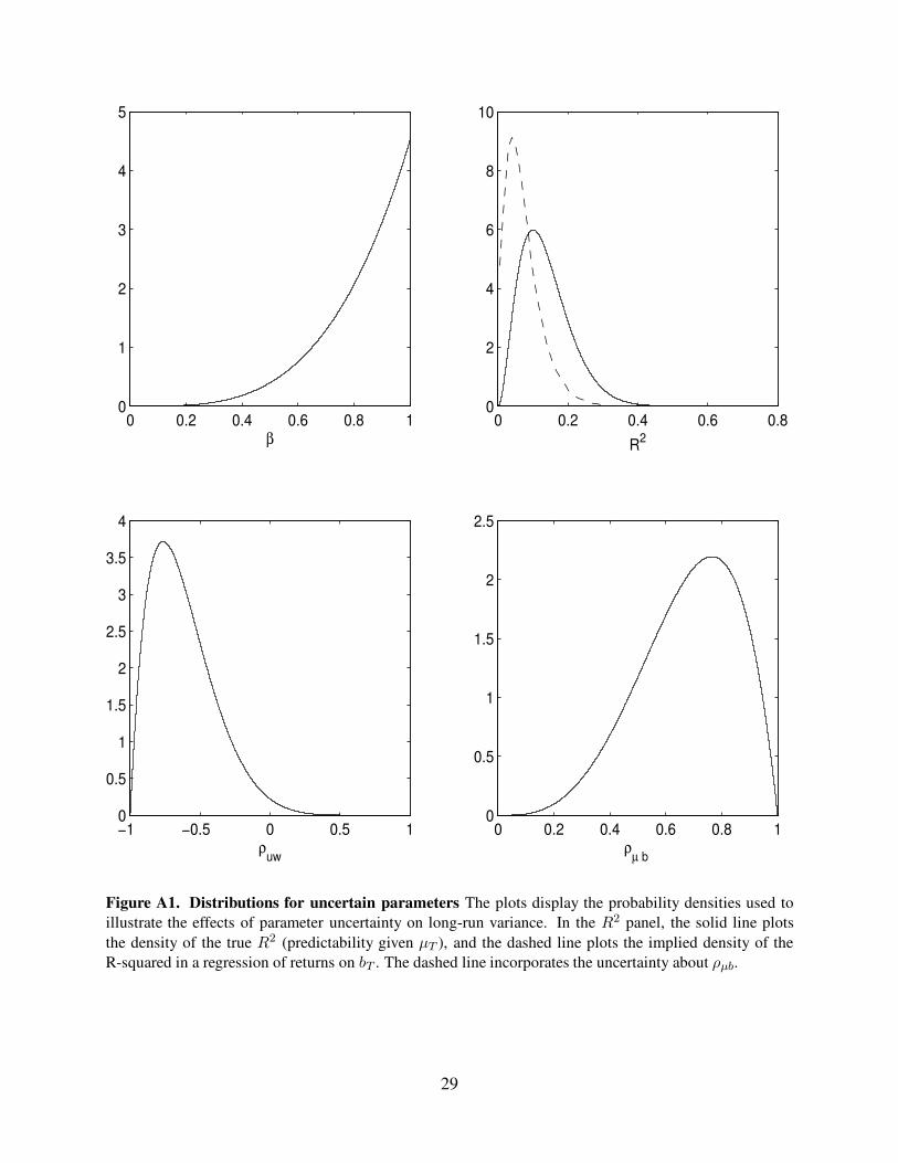
remaining parameters, we choose the probability densities displayed in Figure A1, whose medians
are 0.86 for β, 0.12 for R2, -0.66 for ρuw, and 0.70 for ρµb.
Table A1 displays the 20-year variance ratio, V (20), under different specifications of uncer-
tainty about the parameters. In the first row, β, R2, ρuw, and Er are held fixed, by setting the first
three parameters equal to their medians and by setting τ = 0 in (B2). Successive rows then specify
one or more of those parameters as uncertain, by drawing from the densities in Figure A1 (for β,
R2, and ρuw) or setting τ = 1/200 (forEr). For each row, ρµb is either fixed at one of the values 0,
0.70 (its median), and 1, or it is drawn from its density in Figure A1. Note that the return variances
are unconditional when ρµb = 0 and conditional on full knowledge of µT when ρµb = 1.
Table A1 shows that when all parameters are fixed, V (20) < 1 at all levels of conditioning (all
values of ρµb). That is, in the absence of parameter uncertainty, the values in the first row range
from 0.95 at the unconditional level to 0.77 when µT is fully known. Thus, this fixed-parameter
specification is consistent with mean reversion playing a dominant role, causing the return variance
(per period) to be lower at the long horizon. Rows 2 through 5 specify one of the parameters β,R2,
ρuw, and Er as uncertain. Uncertainty about β exerts the strongest effect, raising V (20) by 17% to
26% (depending on ρµb), but uncertainty about any one of these parameters raises V (20). In the
last row of Table A1, all parameters are uncertain, and the values of V (20) substantially exceed
1, ranging from 1.17 (when ρµb = 1) to 1.45 (when ρµb = 0). Even though the density for ρuw in
Figure A1 has almost all of its mass below 0, so that mean reversion is almost certainly present,
parameter uncertainty causes the long-run variance to exceed the short-run variance.
As discussed in the paper, uncertainty about Er implies V (k) → ∞ as k → ∞. We can see
from Table A1 that uncertainty about Er contributes nontrivially to V (20), but somewhat less than
uncertainty about β or R2 and only slightly more than uncertainty about ρuw. With uncertainty
about only the latter three parameters, V (20) is still well above 1, especially when ρµb < 1. Thus,
although uncertainty about Er must eventually dominate variance at sufficiently long horizons, it
does not do so here at the 20-year horizon.
The variance ratios in Table A1 increase as ρµb decreases. In other words, less knowledge about
µT makes long-run variance greater relative to short-run variance. We also see that drawing ρµb
4

from its density in Figure A1 produces the same values of V (20) as fixing ρµb at its median.
B3. Predictive System 2
System 2 is implemented in the paper for one asset, but it can be specified for n assets, in which
case rt+1 and πt+1 are n× 1 vectors. We begin the analysis with that more general form and then
later restrict it to the single-asset setting. With multiple assets, System 2 is given by
rt+1
xt+1
πt+1
=
aθ0
+
0 A12 I0 A22 00 0 A33
rtxtπt
+
ut+1
vt+1
ηt+1
, (B10)
which can also be written as
rt+1 − Erxt+1 − Exπt+1 − Eπ
=
0 A12 I0 A22 00 0 A33
rt − Erxt − Exπt − Eπ
+
ut+1
vt+1
ηt+1
, (B11)
where Ex = (I − A22)−1θ, Er = a + A12Ex, and without loss of generality Eπ = 0. We begin
working with multiple assets, so that not only xt but also rt and πt are vectors. We assume the
errors in (B11) are i.i.d. across t = 1, . . . , T :
utvtηt
∼ N
000
,
Σuu Σuv Σuη
Σvu Σvv Σvη
Σηu Σηv Σηη
. (B12)
We assume the eigenvalues of both A22 and A33 lie inside the unit circle. As the elements of Σηη
approach zero, the above model approaches the perfect-predictor specification,
[
rt+1 − Erxt+1 − Ex
]
=
[
0 A12
0 A22
] [
rt − Erxt − Ex
]
+
[
ut+1
vt+1
]
. (B13)
Let A denote the entire coefficient matrix in (B11), and let Σ denote the entire covariance
matrix in (B12). Define the vector
ζt =
rtxtπt
, (B14)
and let Vζζ denote its unconditional covariance matrix. Then
Vζζ =
Vrr Vrx VrπVxr Vxx VxπVπr Vπx Vππ
= AVζζA′ + Σ, (B15)
5
which can be solved as
vec (Vζζ) = [I − (A⊗ A)]−1vec (Σ), (B16)
using the well known identity vec (DFG) = (G′ ⊗D)vec (F ).
Let zt denote the vector of the observed data at time t,
zt =
[
rtxt
]
.
Denote the data we observe through time t as Dt = (z1, . . . , zt), and note that our complete data
consist of DT . Also define
Ez =
[
ErEx
]
, Vzz =
[
Vrr VrxVxr Vxx
]
, Vzπ =
[
VrπVxπ
]
. (B17)
Let φ denote the full set of parameters in the model, φ ≡ (A,Σ, Ez), and let π denote the
full time series of πt, t = 1, . . . , T . To obtain the joint posterior distribution of φ and π, denoted
by p(φ, π|DT ), we use an MCMC procedure in which we alternate between drawing π from the
conditional posterior p(π|φ,DT ) and drawing φ from the conditional posterior p(φ|π,DT ). The
procedure for drawing π from p(π|φ,DT ) is described in Section B3.1. The procedure for drawing
φ from p(φ|π,DT ) ∝ p(φ)p(DT , π|φ) is described in Section B3.2.
B3.1. Drawing π given the parameters
To draw the time series of the unobservable values of πt conditional on the current parameter
draws, we apply the forward filtering, backward sampling (FFBS) approach developed by Carter
and Kohn (1994) and Fruhwirth-Schnatter (1994). See also West and Harrison (1997, chapter 15).
B3.1.1. Filtering
The first stage follows the standard methodology of Kalman filtering. Define
at = E(πt|Dt−1) bt = E(πt|Dt) et = E(zt|πt, Dt−1) (B18)
ft = E(zt|Dt−1) Pt = Var(πt|Dt−1) Qt = Var(πt|Dt) (B19)
Rt = Var(zt|πt, Dt−1) St = Var(zt|Dt−1) Gt = Cov(zt, π′
t|Dt−1) (B20)
Conditioning on φ is assumed throughout this section but suppressed in the notation for conve-
nience. First observe that
π1|D0 ∼ N(a1, P1), (B21)
6

where D0 denotes the null information set, so that the unconditional moments of π0 are given by
a1 = Eπ = 0 and P1 = Vππ . Also,
z1|D0 ∼ N(f1, S1), (B22)
where f1 = Ez and S1 = Vzz . Note that
G1 = Vzπ (B23)
and that
z1|π1, D0 ∼ N(e1, R1), (B24)
where
e1 = f1 +G1P−11 (π1 − a1) (B25)
R1 = S1 −G1P−11 G′
1. (B26)
Combining this density with equation (B21) using Bayes rule gives
π1|D1 ∼ N(b1, Q1), (B27)
where
b1 = a1 + P1(P1 + G′
1R−11 G1)
−1G′
1R−11 (z1 − f1) (B28)
Q1 = P1(P1 +G′
1R−11 G1)
−1P1. (B29)
Continuing in this fashion, we find that all conditional densities are normally distributed, and we
obtain all the required moments for t = 2, . . . , T :
at = A33bt−1 (B30)
ft =
[
Er + A12(xt−1 −Ex) + bt−1
Ex + A22(xt−1 − Ex)
]
(B31)
St =
[
Qt−1 00 0
]
+
[
Σuu Σuv
Σvu Σvv
]
(B32)
Gt =
[
Qt−1A′
33
0
]
+
[
Σuη
Σvη
]
(B33)
Pt = A33Qt−1A′
33 + Σηη (B34)
et = ft +GtP−1t (πt − at) (B35)
Rt = St −GtP−1t G′
t (B36)
bt = at + Pt(Pt +G′
tR−1t Gt)
−1G′
tR−1t (zt − ft) (B37)
= at +G′
tS−1t (zt − ft) (B38)
Qt = Pt(Pt +G′
tR−1t Gt)
−1Pt. (B39)
7
The values of at, bt, Qt, St, Gt, Pt for t = 1, . . . , T are retained for the next stage. Equations
(B32) through (B34) are derived as
[
St Gt
G′
t Pt
]
= Var(ζt|Dt−1)
= AVar(ζt−1|Dt−1)A′ + Σ
= A
0 0 00 0 00 0 Qt−1
A′ + Σ
=
Qt−1 0 Qt−1A′
33
0 0 0A33Qt−1 0 A33Qt−1A
′
33
+
Σuu Σuv Σuη
Σvu Σvv Σvη
Σηu Σηv Σηη
.
B3.1.2. Sampling—drawing π
We wish to draw (π1, . . . , πT ) conditional on DT (and the parameters, φ). The backward-
sampling approach relies on the Markov property of the evolution of ζt and the resulting identity,
p(ζ1, . . . , ζT |DT ) = p(ζT |DT )p(ζT−1|ζT , DT−1) · · · p(ζ1|ζ2, D1). (B40)
We first sample πT from p(πT |DT ), the normal density obtained in the last step of the filtering.
Then, for t = T − 1, T − 2, . . . , 1, we sample πt from the conditional density p(ζt|ζt+1, Dt). (Note
that the first two subvectors of ζt are already observed and thus need not be sampled.) To obtain
that conditional density, first note that
ζt+1|Dt ∼ N
([
ft+1
at+1
]
,
[
St+1 Gt+1
G′
t+1 Pt+1
])
, (B41)
ζt|Dt ∼ N
rtxtbt
,
0 0 00 0 00 0 Qt
, (B42)
and
Cov(ζt, ζ′
t+1|Dt) = Var(ζt|Dt)A′
=
0 0 00 0 00 0 Qt
0 0 0A′
12 A′
22 0I 0 A′
33
=
0 0 00 0 0Qt 0 QtA
′
33
. (B43)
8
Therefore,
ζt|ζt+1, Dt ∼ N(ht, Ht), (B44)
where
ht = E(ζt|Dt) +[
Cov(ζt, ζ′
t+1|Dt)]
[Var(ζt+1|Dt)]−1 [ζt+1 − E(ζt+1|Dt)]
=
rtxtbt
+
0 0 00 0 0Qt 0 QtA
′
33
[
St+1 Gt+1
G′
t+1 Pt+1
]
−1 [
zt+1 − ft+1
πt+1 − at+1
]
and
Ht = Var(ζt|Dt) −[
Cov(ζt, ζ′
t+1|Dt)]
[Var(ζt+1|Dt)]−1[
Cov(ζt, ζ′
t+1|Dt)]
′
=
0 0 00 0 00 0 Qt
−
0 0 00 0 0Qt 0 QtA
′
33
[
St+1 Gt+1
G′
t+1 Pt+1
]
−1
0 0 Qt
0 0 00 0 A33Qt
The mean and covariance matrix of πt are taken as the relevant elements of ht and Ht.
In the rest of the Appendix, we discuss the special case (implemented in the paper) in which rt
and πt are scalars. The dimensions of A and Σ are then (K+2)× (K+2), whereK is the number
of predictors in the vector xt. In this case, A′
12 is a K × 1 vector, which we denote as b (distinct
from bt, defined previously), and A33 is a scalar that we denote as δ. We also denote A22 as simply
A (distinct from A, defined previously).
B3.2. Drawing the parameters given π
B3.2.1. Prior distributions
With rt and πt being scalars,
Σ =
σ2u σuv σuη
σvu Σvv σvησηu σηv σ2
η
=
[
Σξξ σξησ′
ξη σ2η
]
,
where ξ′t ≡ [ut v′
t]. We wish to be informative about σ2η , to varying degrees, while being nonin-
formative about Σξξ and σξη. This objective is accomplished by specifying a prior for Σ equal to
the posterior that obtains when a diffuse prior for Σ is combined with a hypothetical sample of
T0 observations of ηt and S0 observations of ξt, where S0 ≤ T0 and the shorter period is a subset
of the longer. This posterior is given by Stambaugh (1997), except that we impose the additional
restriction that the population means of ηt and ξt are zero. The posterior in Stambaugh (1997)
9
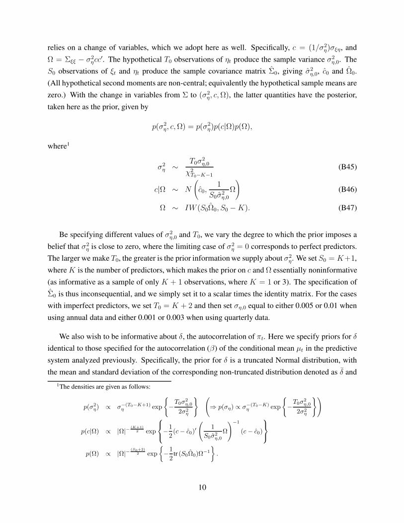
relies on a change of variables, which we adopt here as well. Specifically, c = (1/σ2η)σξη, and
Ω = Σξξ − σ2ηcc
′. The hypothetical T0 observations of ηt produce the sample variance σ2η,0. The
S0 observations of ξt and ηt produce the sample covariance matrix Σ0, giving σ2η,0, c0 and Ω0.
(All hypothetical second moments are non-central; equivalently the hypothetical sample means are
zero.) With the change in variables from Σ to (σ2η, c,Ω), the latter quantities have the posterior,
taken here as the prior, given by
p(σ2η, c,Ω) = p(σ2
η)p(c|Ω)p(Ω),
where1
σ2η ∼
T0σ2η,0
χ2T0−K−1
(B45)
c|Ω ∼ N
(
c0,1
S0σ2η,0
Ω
)
(B46)
Ω ∼ IW (S0Ω0, S0 −K). (B47)
Be specifying different values of σ2η,0 and T0, we vary the degree to which the prior imposes a
belief that σ2η is close to zero, where the limiting case of σ2
η = 0 corresponds to perfect predictors.
The larger we make T0, the greater is the prior information we supply about σ2η. We set S0 = K+1,
whereK is the number of predictors, which makes the prior on c and Ω essentially noninformative
(as informative as a sample of only K + 1 observations, where K = 1 or 3). The specification of
Σ0 is thus inconsequential, and we simply set it to a scalar times the identity matrix. For the cases
with imperfect predictors, we set T0 = K + 2 and then set ση,0 equal to either 0.005 or 0.01 when
using annual data and either 0.001 or 0.003 when using quarterly data.
We also wish to be informative about δ, the autocorrelation of πt. Here we specify priors for δ
identical to those specified for the autocorrelation (β) of the conditional mean µt in the predictive
system analyzed previously. Specifically, the prior for δ is a truncated Normal distribution, with
the mean and standard deviation of the corresponding non-truncated distribution denoted as δ and
1The densities are given as follows:
p(σ2η) ∝ σ−(T0−K+1)
η exp
−T0σ
2η,0
2σ2η
(
⇒ p(ση) ∝ σ−(T0−K)η exp
−T0σ
2η,0
2σ2η
)
p(c|Ω) ∝ |Ω|−(K+1)
2 exp
−1
2(c − c0)
′
(
1
S0σ2η,0
Ω
)
−1
(c − c0)
p(Ω) ∝ |Ω|−(S0+2)
2 exp
−1
2tr (S0Ω0)Ω
−1
.
10
σδ. The distribution is then truncated to satisfy the stationarity requirement |δ| < 1. We set σδ to
0.25 with annual data and to 0.15 with quarterly data, and we set δ to 0.99 in both cases.
The priors on the remaining parameters are non-informative, except for the condition required
for stationary of xt that ρ(A), the spectral radius of A, be less than 1. Specifically, define
ψ =
vec
[
a θ′
b A′
]
δ
. (B48)
Then the prior for ψ is given by
p(ψ) ∝ exp
−1
2(ψ − ψ)′V −1
ψ (ψ − ψ)
× 1S , (B49)
where
ψ =
[
0δ
]
, Vψ =
[
σ2ψI(K+1)2 0
0 σ2δ
]
, (B50)
σ2ψ is set to a large number, 1S equals 1 under the conditions that ρ(A) < 1 and |δ| < 1, and 1S
equals 0 otherwise. We also assume that the priors for Σ and ψ are independent.
B3.2.2. Posterior distributions
Define
yt+1 =
rt+1 − πtxt+1
πt+1
, Yt =
[
IK+1 ⊗ [1 x′t] 00 πt
]
, υt+1 =
ut+1
vt+1
ηt+1
,
y =
y2...
yT
, Y =
Y1...
YT−1
, υ =
υ2...
υT
.
The sample representation of the predictive system in (B10) is then
y = Y ψ + υ,
for ψ defined in (B48). For tractability we employ the “conditional” likelihood, which treats values
in period t = 1 as non-stochastic. We can then apply Gibbs sampling to draw ψ and Σ. This
simplification seems reasonable, given that T = 206 for our main results.2
2An alternative would be to employ the “exact” likelihood that includes the density of the values at t = 1 and then
use the Metropolis-Hastings algorithm, with the conditional posteriors given here used as proposal densities.
11
B3.2.3. Drawing ψ
Given the prior for ψ in (B49), we can apply standard results from the multivariate regression
model (e.g., Zellner, 1971) to obtain the full conditional posterior for ψ as
ψ|· ∼ N(ψ, Vψ) × 1S (B51)
where
ψ = Vψ[
V −1ψ ψ + Y ′(IT−1 ⊗ Σ−1)y
]
and
Vψ =[
V −1ψ + Y ′(IT−1 ⊗ Σ−1)Y
]
−1
.
B3.2.4. Drawing Σ
Define
Σ =1
T − 1
T−1∑
t=1
(yt+1 − Ytψ)(yt+1 − Ytψ)′ =
[
Σξξ σξησ′
ξη σ2η
]
Σ =
[
Σξξ σξησ′
ξη σ2η
]
=1
S
(
S0Σ0 + (T − 1)Σ)
, S = S0 + (T − 1)
c = (1/σ2η)σξη, Ω = Σξξ − σ2
η cc′,
σ2η =
1
T
(
T0σ2η,0 + (T − 1)σ2
η
)
, T = T0 + (T − 1).
A draw of Σ is constructed by drawing (σ2η, c,Ω). The joint full conditional of the latter is given
by
p(σ2η , c,Ω|·) = p(σ2
η |·)p(c|Ω, ·)p(Ω|·),
where the posteriors on the right-hand side are of the same form as (B45) through (B47):
σ2η|· ∼
T σ2η
χ2T−K−1
(B52)
c|Ω, · ∼ N
(
c,1
Sσ2η
Ω
)
(B53)
Ω|· ∼ IW (SΩ, S −K). (B54)
The draw of Σ is then obtained by computing Σξξ = Ω + σ2ηcc
′ and σξη = σ2ηc.
Our results based on 25,000 draws from the posterior distribution. First, we generate a sequence
of 76,000 draws. We discard the first 1,000 draws as a “burn-in” and take every third draw from
the rest to obtain a series of 25,000 draws that exhibit little serial correlation.
12
B3.3. Predictive variance
In addition to the notation from equations (B11), (B12), and (B14), define also
Eζ =
ErEx0
, εt =
utvtηt
, (B55)
and
ζet = ζt − Eζ . (B56)
Equation (B11) can then be written as
ζet+1 = Aζet + εt+1. (B57)
For i > 1, successive substitution using (B57) gives
ζet+i = Aiζet + Ai−1εt+1 + Ai−2εt+2 + · · · + εt+i. (B58)
Define
ζT,T+k =k∑
i=1
ζT+i,
ζeT,T+k =k∑
i=1
ζeT+i = ζT,T+k − kEζ .
Summing (B57) over k periods then gives
ζeT,T+k =
(
k∑
i=1
Ai
)
ζet +(
I + A+ · · · + Ak−1)
εt+1
+(
I + A + · · · + Ak−2)
εt+2 + · · · + εt+k
= (Λk+1 − I)ζet + Λkεt+1 + Λk−1εt+2 + · · · + εt+k, (B59)
where
Λi = I + A+ · · · + Ai−1
= (I − A)−1(I − Ai). (B60)
It then follows that
E(
ζeT,T+k|DT , φ, πT)
= (Λk+1 − I)ζeT ,
E (ζT,T+k|DT , φ, πT ) = (Λk+1 − I)ζeT + kEζ , (B61)
13
and
Var (ζT,T+k|DT , φ, πT ) = Var(
ζeT,T+k|DT , φ, πT)
=k∑
i=1
ΛiΣΛ′
i. (B62)
The first and second moments of (B61) given DT and φ are given by
E (ζT,T+k|DT , φ) = (Λk+1 − I)
rT −ErxT − ExbT
+ kEζ (B63)
and
Var [E (ζT,T+k|DT , φ, πT ) |DT , φ] = (Λk+1 − I)
0 0 00 0 00 0 QT
(Λk+1 − I)′. (B64)
Combining (B62) and (B64) gives
Var (ζT,T+k|DT , φ) = E [Var (ζT,T+k|DT , φ, πT) |DT , φ] + Var [E (ζT,T+k|DT , φ, πT ) |DT , φ]
=k∑
i=1
ΛiΣΛ′
i + (Λk+1 − I)
0 0 00 0 00 0 QT
(Λk+1 − I)′. (B65)
By evaluating (B63) and (B65) for repeated draws of φ from its posterior, the predictive variance
of ζT,T+k can be computed using the decomposition,
Var(ζT,T+k|DT ) = E Var(ζT,T+k|φ,DT )|DT + Var E(ζT,T+k|φ,DT )|DT . (B66)
Finally, the predictive variance of rT,T+k is the (1,1) element of Var(ζT,T+k|DT ).
B3.4. Perfect predictors
If the predictors are perfect, then πt is absent from the first equation in (B10) and the third equation
simply drops out. In that case the model consists of the two equations,
rt+1 = a + b′xt + ut+1 (B67)
xt+1 = θ + Axt + vt+1, (B68)
combined with the distributional assumption on the residuals,
[
utvt
]
∼ N
([
00
]
,
[
σ2u σuv
σvu Σvv
])
. (B69)
14
This perfect-predictor model obtains as the limiting case of the above imperfect-predictor setting
as σ2η → 0. Our perfect-predictor results can be computed in that manner, by setting T0 to a large
number and ση,0 to a small number. For completeness, however, we also provide here the simplified
calculations that arise in that special case.
In this case φ denotes the full set of parameters in equations (B75), (B68), and (B69), and Σ
denotes the covariance matrix in (B69). Let B denote the matrix of coefficients in (B75) and (B68),
B =
[
a θ′
b A′
]
,
and let ψ = vec (B).
B3.4.1. Posterior distributions under perfect predictors
We specify the prior distribution on φ as p(φ) = p(ψ)p(Σ). The prior on ψ is p(ψ) ∝ 1S , where
1S equals 1 if ρ(A) < 1 and equals 0 otherwise. The prior on Σ is p(Σ) ∝ |Σ|−(K+2)/2. Define
the following notation: r = [r2 r3 · · · rT ]′
, Q+ = [x2 x3 · · · xT ]′
, Q = [x1 x2 · · · xT−1]′
, X =
[ιT−1 Q], where ιT−1 denotes a (T − 1) × 1 vector of ones, Y = [r Q+], B = (X ′X)−1X ′Y ,
and S = (Y − XB)′(Y −XB). We first draw Σ−1 from a Wishart distribution with T −K − 2
degrees of freedom and parameter matrix S−1. Given that draw of Σ−1, we then draw ψ from a
normal distribution with mean ψ = vec (B) and covariance matrix Σ ⊗ (X ′X)−1. That draw of φ
is retained as a draw from p(φ|DT ) if ρ(A) < 1.
B3.4.2. Predictive variance under perfect predictors
The conditional moments of the k-period return rT,T+k are given by
E(rT,T+k|DT , φ) = ka+ b′Ψk−1θ + b′ΛkxT (B70)
Var(rT,T+k|DT , φ) = kσ2u + 2b′Ψk−1σvu + b′
(
k−1∑
i=1
ΛiΣvvΛ′
i
)
b, (B71)
where
Λi = I + A + · · · + Ai−1 = (I − A)−1(I − Ai) (B72)
Ψk−1 = Λ1 + Λ2 + · · · + Λk−1 = (I − A)−1[kI − (I −A)−1(I −Ak)]. (B73)
The first term in (B71) reflects i.i.d. uncertainty. The second term reflects correlation between
unexpected returns and innovations in future xT+i’s, which deliver innovations in future µT+i’s.
15
That term can be positive or negative and captures any mean reversion. The third term, always
positive, reflects uncertainty about future xT+i’s, and thus uncertainty about future µT+i’s. This
third term, which contains a summation, can also be written without the summation as
b′(
k−1∑
i=1
ΛiΣvvΛ′
i
)
b = (b′ ⊗ b′)[
(I − A)−1 ⊗ (I − A)−1] [
kI − Λk ⊗ I − I ⊗ Λk
+(I − A⊗ A)−1(I − (A⊗A)k)]
vec (Σvv) .
Applying the standard variance decomposition
Var(rT,T+k|DT ) = EVar(rT,T+k|DT , φ)|DT + VarE(rT,T+k|DT , φ)|DT, (B74)
the predictive variance Var(rT,T+k|DT ) can be computed as the sum of the posterior mean of the
right-hand side of equation (B71) and the posterior variance of the right-hand side of equation
(B70). These posterior moments are computed from the posterior draws of φ, which are described
in Section B3.4.1.
B4. Additional empirical results
B4.1. Predictive regressions
This section reports the results from standard predictive regressions,
rt+1 = a + b′xt + et+1 , (B75)
for various combinations of the three predictors used in the paper. The results, obtained by OLS,
are reported in Table A2. Panel A reports the results based on annual data; the results based on
quarterly data are reported in Panel B. In both panels, the first three regressions contain just one
predictor, while the fourth regression contains all three. The table reports the estimated coefficients
as well as the t-statistics, along with the bootstrapped p-values associated with these t-statistics as
well as with the R2.3
3In the bootstrap, we repeat the following procedure 20,000 times: (i) Resample T pairs of (vt, et), with replace-
ment, from the set of OLS residuals from regressions (B68) and (B75); (ii) Build up the time series of xt, starting from
the unconditional mean and iterating forward on equation (B68), using the OLS estimates (θ, A) and the resampled
values of vt; (iii) Construct the time series of returns, rt, by adding the resampled values of et to the sample mean
(i.e., under the null that returns are not predictable); (iv) Use the resulting series of xt and rt to estimate regressions
(B68) and (B75) by OLS. The bootstrapped p-value associated with the reported t-statistic (or R2) is the relative
frequency with which the reported quantity is smaller than its 20,000 counterparts bootstrapped under the null of no
predictability.
16

Table A2 shows that all the predictors exhibit significant ability to predict returns, especially
in the multivariate regressions that involve all three predictors. In those regressions, the estimated
correlation between et+1 and the estimated innovation in expected return, b′vt+1, is negative. Pastor
and Stambaugh (2009) suggest this correlation as a diagnostic in predictive regressions, with a
negative value being what one would hope to see for predictors able to deliver a reasonable proxy
for expected return.
B4.2. Long-horizon predictive variance
This section provides detailed robustness results on the long-horizon predictive variance, expand-
ing the evidence reported in the paper for both predictive systems. We examine the following
cases:
Annual data: Baseline case reported in the paper
System 1: Table A3; Figures A2, A3
System 2: Figure A18, left column
Annual data: First subperiod
System 1: Table A4; Figures A4, A5
System 2: Figure A19, left column
Annual data: Second subperiod
System 1: Table A5; Figures A6, A7
System 2: Figure A19, right column
Annual data: One instead of three predictors
System 1: Table A6; Figures A8, A9
System 2: Figure A20, left column
Annual data: Excess instead of real returns
System 1: Table A7; Figures A10, A11
System 2: Figure A21, left column
Quarterly data: Baseline case reported in the paper
System 1: Table A8; Figures A12, A13
System 2: Figure A18, right column
Quarterly data: One instead of three predictors
System 1: Table A9; Figures A14, A15
System 2: Figure A20, right column
Quarterly data: Excess instead of real returns
System 1: Table A10; Figures A16, A17
17

System 2: Figure A21, right column
We do not report subperiod results for quarterly data because the (post-war) quarterly sample
is already rather short compared to the 206-year annual sample. Parameter uncertainty generally
plays a larger role in shorter samples.
18
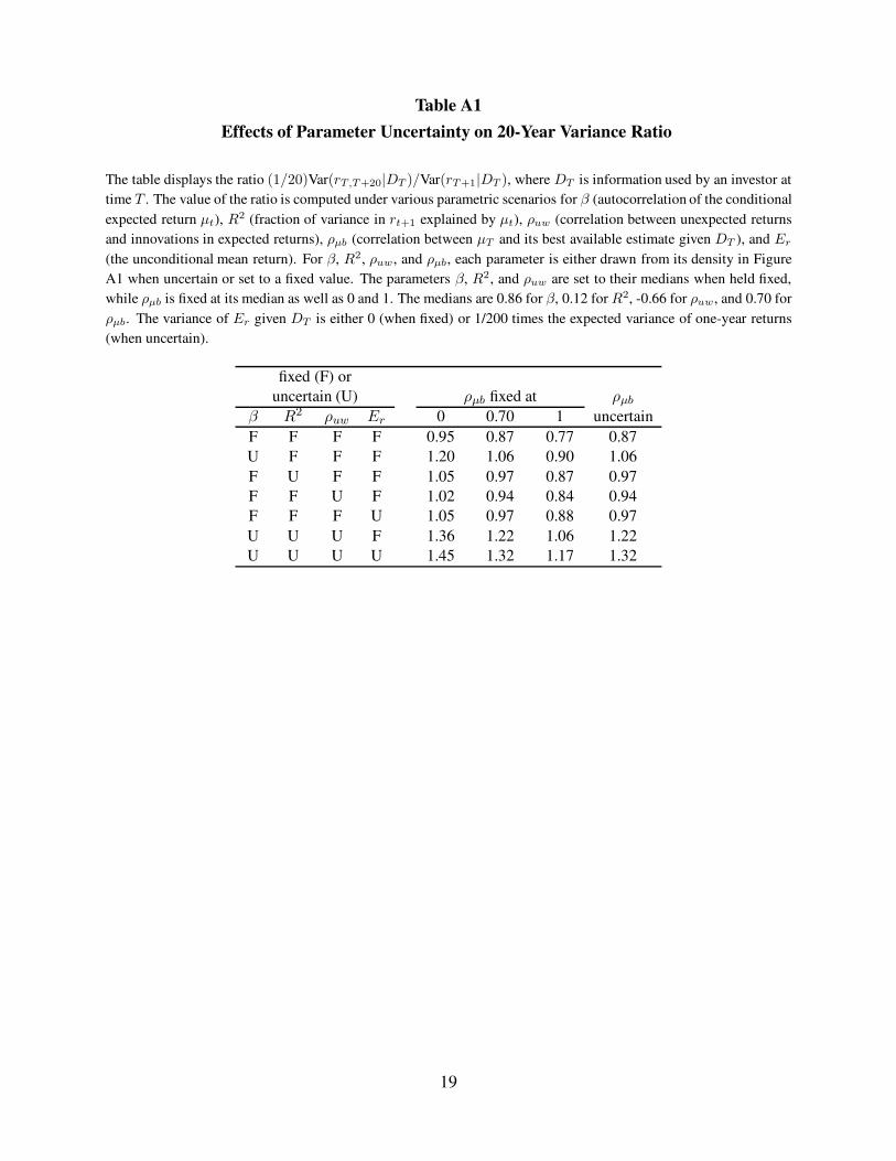
Table A1
Effects of Parameter Uncertainty on 20-Year Variance Ratio
The table displays the ratio (1/20)Var(rT,T+20|DT )/Var(rT+1|DT ), where DT is information used by an investor at
time T . The value of the ratio is computed under various parametric scenarios for β (autocorrelation of the conditional
expected return µt), R2 (fraction of variance in rt+1 explained by µt), ρuw (correlation between unexpected returns
and innovations in expected returns), ρµb (correlation between µT and its best available estimate given DT ), and Er
(the unconditional mean return). For β, R2, ρuw, and ρµb, each parameter is either drawn from its density in Figure
A1 when uncertain or set to a fixed value. The parameters β, R2, and ρuw are set to their medians when held fixed,
while ρµb is fixed at its median as well as 0 and 1. The medians are 0.86 for β, 0.12 for R2, -0.66 for ρuw, and 0.70 for
ρµb. The variance of Er given DT is either 0 (when fixed) or 1/200 times the expected variance of one-year returns
(when uncertain).
fixed (F) or
uncertain (U) ρµb fixed at ρµbβ R2 ρuw Er 0 0.70 1 uncertain
F F F F 0.95 0.87 0.77 0.87
U F F F 1.20 1.06 0.90 1.06
F U F F 1.05 0.97 0.87 0.97
F F U F 1.02 0.94 0.84 0.94
F F F U 1.05 0.97 0.88 0.97
U U U F 1.36 1.22 1.06 1.22
U U U U 1.45 1.32 1.17 1.32
19
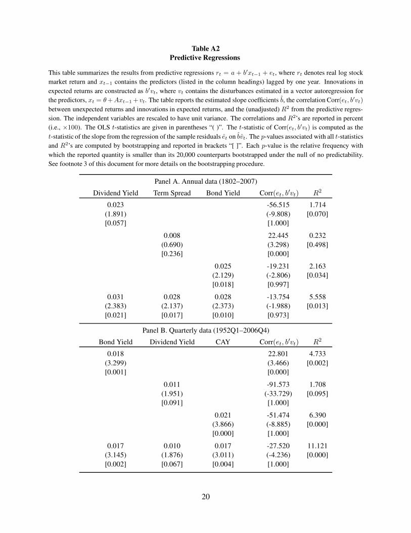
Table A2
Predictive Regressions
This table summarizes the results from predictive regressions rt = a + b′xt−1 + et, where rt denotes real log stock
market return and xt−1 contains the predictors (listed in the column headings) lagged by one year. Innovations in
expected returns are constructed as b′vt, where vt contains the disturbances estimated in a vector autoregression for
the predictors, xt = θ +Axt−1 + vt. The table reports the estimated slope coefficients b, the correlation Corr(et, b′vt)
between unexpected returns and innovations in expected returns, and the (unadjusted) R2 from the predictive regres-
sion. The independent variables are rescaled to have unit variance. The correlations and R2’s are reported in percent
(i.e., ×100). The OLS t-statistics are given in parentheses “( )”. The t-statistic of Corr(et, b′vt) is computed as the
t-statistic of the slope from the regression of the sample residuals et on bvt. The p-values associated with all t-statistics
and R2’s are computed by bootstrapping and reported in brackets “[ ]”. Each p-value is the relative frequency with
which the reported quantity is smaller than its 20,000 counterparts bootstrapped under the null of no predictability.
See footnote 3 of this document for more details on the bootstrapping procedure.
Panel A. Annual data (1802–2007)
Dividend Yield Term Spread Bond Yield Corr(et, b′vt) R2
0.023 -56.515 1.714
(1.891) (-9.808) [0.070]
[0.057] [1.000]
0.008 22.445 0.232
(0.690) (3.298) [0.498]
[0.236] [0.000]
0.025 -19.231 2.163
(2.129) (-2.806) [0.034]
[0.018] [0.997]
0.031 0.028 0.028 -13.754 5.558
(2.383) (2.137) (2.373) (-1.988) [0.013]
[0.021] [0.017] [0.010] [0.973]
Panel B. Quarterly data (1952Q1–2006Q4)
Bond Yield Dividend Yield CAY Corr(et, b′vt) R2
0.018 22.801 4.733
(3.299) (3.466) [0.002]
[0.001] [0.000]
0.011 -91.573 1.708
(1.951) (-33.729) [0.095]
[0.091] [1.000]
0.021 -51.474 6.390
(3.866) (-8.885) [0.000]
[0.000] [1.000]
0.017 0.010 0.017 -27.520 11.121
(3.145) (1.876) (3.011) (-4.236) [0.000]
[0.002] [0.067] [0.004] [1.000]
20
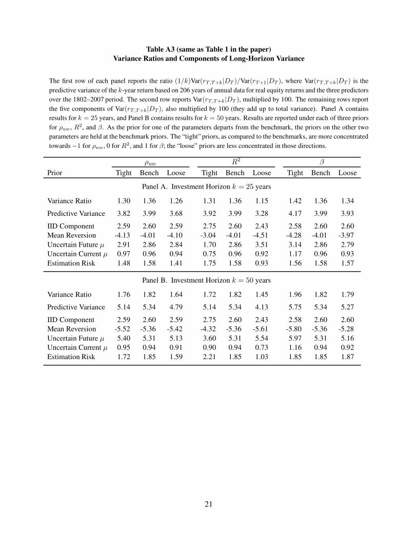
Table A3 (same as Table 1 in the paper)
Variance Ratios and Components of Long-Horizon Variance
The first row of each panel reports the ratio (1/k)Var(rT,T+k|DT )/Var(rT+1|DT ), where Var(rT,T+k|DT ) is the
predictive variance of the k-year return based on 206 years of annual data for real equity returns and the three predictors
over the 1802–2007 period. The second row reports Var(rT,T+k|DT ), multiplied by 100. The remaining rows report
the five components of Var(rT,T+k|DT ), also multiplied by 100 (they add up to total variance). Panel A contains
results for k = 25 years, and Panel B contains results for k = 50 years. Results are reported under each of three priors
for ρuw, R2, and β. As the prior for one of the parameters departs from the benchmark, the priors on the other two
parameters are held at the benchmark priors. The “tight” priors, as compared to the benchmarks, are more concentrated
towards −1 for ρuw, 0 for R2, and 1 for β; the “loose” priors are less concentrated in those directions.
ρuw R2 β
Prior Tight Bench Loose Tight Bench Loose Tight Bench Loose
Panel A. Investment Horizon k = 25 years
Variance Ratio 1.30 1.36 1.26 1.31 1.36 1.15 1.42 1.36 1.34
Predictive Variance 3.82 3.99 3.68 3.92 3.99 3.28 4.17 3.99 3.93
IID Component 2.59 2.60 2.59 2.75 2.60 2.43 2.58 2.60 2.60
Mean Reversion -4.13 -4.01 -4.10 -3.04 -4.01 -4.51 -4.28 -4.01 -3.97
Uncertain Future µ 2.91 2.86 2.84 1.70 2.86 3.51 3.14 2.86 2.79
Uncertain Current µ 0.97 0.96 0.94 0.75 0.96 0.92 1.17 0.96 0.93
Estimation Risk 1.48 1.58 1.41 1.75 1.58 0.93 1.56 1.58 1.57
Panel B. Investment Horizon k = 50 years
Variance Ratio 1.76 1.82 1.64 1.72 1.82 1.45 1.96 1.82 1.79
Predictive Variance 5.14 5.34 4.79 5.14 5.34 4.13 5.75 5.34 5.27
IID Component 2.59 2.60 2.59 2.75 2.60 2.43 2.58 2.60 2.60
Mean Reversion -5.52 -5.36 -5.42 -4.32 -5.36 -5.61 -5.80 -5.36 -5.28
Uncertain Future µ 5.40 5.31 5.13 3.60 5.31 5.54 5.97 5.31 5.16
Uncertain Current µ 0.95 0.94 0.91 0.90 0.94 0.73 1.16 0.94 0.92
Estimation Risk 1.72 1.85 1.59 2.21 1.85 1.03 1.85 1.85 1.87
21
Table A4
Variance Ratios and Components of Long-Horizon Variance
First subperiod (1802–1904)
Counterpart of Table A3
ρuw R2 β
Prior Tight Bench Loose Tight Bench Loose Tight Bench Loose
Panel A. Investment Horizon k = 25 years
Variance Ratio 1.28 1.35 1.38 1.46 1.35 1.22 1.27 1.35 1.55
Predictive Variance 2.86 3.00 3.05 3.30 3.00 2.65 2.80 3.00 3.48
IID Component 2.01 2.01 2.02 2.11 2.01 1.92 1.96 2.01 2.04
Mean Reversion -1.99 -1.71 -1.44 -1.32 -1.71 -1.92 -2.37 -1.71 -1.39
Uncertain Future µ 1.17 1.13 1.09 0.66 1.13 1.49 1.69 1.13 0.92
Uncertain Current µ 0.36 0.34 0.28 0.30 0.34 0.28 0.57 0.34 0.28
Estimation Risk 1.31 1.23 1.09 1.56 1.23 0.87 0.95 1.23 1.64
Panel B. Investment Horizon k = 50 years
Variance Ratio 1.70 1.78 1.79 2.00 1.78 1.55 1.66 1.78 2.16
Predictive Variance 3.80 3.96 3.97 4.54 3.96 3.35 3.64 3.96 4.86
IID Component 2.01 2.01 2.02 2.11 2.01 1.92 1.96 2.01 2.04
Mean Reversion -2.49 -2.15 -1.81 -1.76 -2.15 -2.31 -3.06 -2.15 -1.74
Uncertain Future µ 2.04 2.00 1.91 1.35 2.00 2.34 3.02 2.00 1.64
Uncertain Current µ 0.40 0.37 0.31 0.39 0.37 0.25 0.59 0.37 0.32
Estimation Risk 1.84 1.73 1.54 2.44 1.73 1.16 1.13 1.73 2.60
22
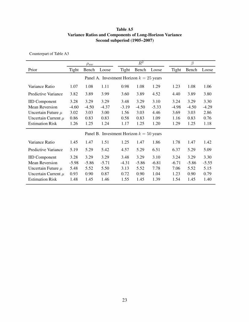
Table A5
Variance Ratios and Components of Long-Horizon Variance
Second subperiod (1905–2007)
Counterpart of Table A3
ρuw R2 β
Prior Tight Bench Loose Tight Bench Loose Tight Bench Loose
Panel A. Investment Horizon k = 25 years
Variance Ratio 1.07 1.08 1.11 0.98 1.08 1.29 1.23 1.08 1.06
Predictive Variance 3.82 3.89 3.99 3.60 3.89 4.52 4.40 3.89 3.80
IID Component 3.28 3.29 3.29 3.48 3.29 3.10 3.24 3.29 3.30
Mean Reversion -4.60 -4.50 -4.37 -3.19 -4.50 -5.33 -4.98 -4.50 -4.29
Uncertain Future µ 3.02 3.03 3.00 1.56 3.03 4.46 3.69 3.03 2.86
Uncertain Current µ 0.86 0.83 0.83 0.58 0.83 1.09 1.16 0.83 0.76
Estimation Risk 1.26 1.25 1.24 1.17 1.25 1.20 1.29 1.25 1.18
Panel B. Investment Horizon k = 50 years
Variance Ratio 1.45 1.47 1.51 1.25 1.47 1.86 1.78 1.47 1.42
Predictive Variance 5.19 5.29 5.42 4.57 5.29 6.51 6.37 5.29 5.09
IID Component 3.28 3.29 3.29 3.48 3.29 3.10 3.24 3.29 3.30
Mean Reversion -5.98 -5.86 -5.71 -4.31 -5.86 -6.81 -6.71 -5.86 -5.55
Uncertain Future µ 5.48 5.52 5.50 3.13 5.52 7.78 7.06 5.52 5.15
Uncertain Current µ 0.93 0.90 0.87 0.72 0.90 1.04 1.23 0.90 0.79
Estimation Risk 1.48 1.45 1.46 1.55 1.45 1.39 1.54 1.45 1.40
23
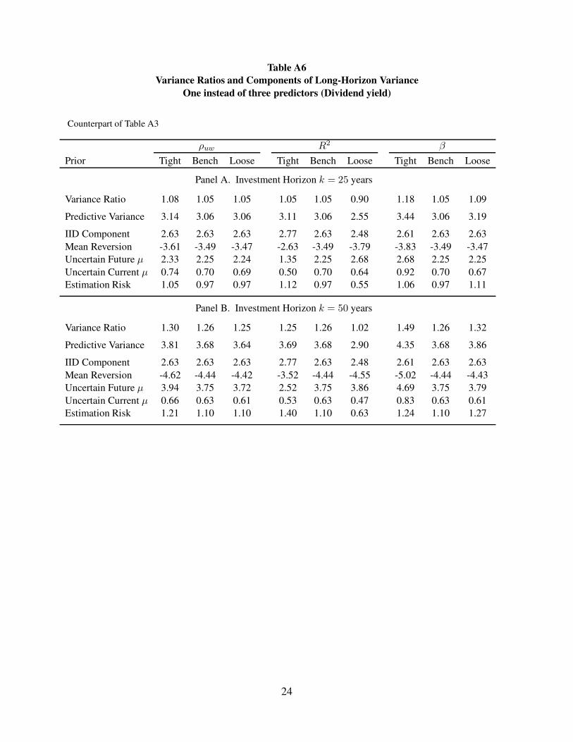
Table A6
Variance Ratios and Components of Long-Horizon Variance
One instead of three predictors (Dividend yield)
Counterpart of Table A3
ρuw R2 β
Prior Tight Bench Loose Tight Bench Loose Tight Bench Loose
Panel A. Investment Horizon k = 25 years
Variance Ratio 1.08 1.05 1.05 1.05 1.05 0.90 1.18 1.05 1.09
Predictive Variance 3.14 3.06 3.06 3.11 3.06 2.55 3.44 3.06 3.19
IID Component 2.63 2.63 2.63 2.77 2.63 2.48 2.61 2.63 2.63
Mean Reversion -3.61 -3.49 -3.47 -2.63 -3.49 -3.79 -3.83 -3.49 -3.47
Uncertain Future µ 2.33 2.25 2.24 1.35 2.25 2.68 2.68 2.25 2.25
Uncertain Current µ 0.74 0.70 0.69 0.50 0.70 0.64 0.92 0.70 0.67
Estimation Risk 1.05 0.97 0.97 1.12 0.97 0.55 1.06 0.97 1.11
Panel B. Investment Horizon k = 50 years
Variance Ratio 1.30 1.26 1.25 1.25 1.26 1.02 1.49 1.26 1.32
Predictive Variance 3.81 3.68 3.64 3.69 3.68 2.90 4.35 3.68 3.86
IID Component 2.63 2.63 2.63 2.77 2.63 2.48 2.61 2.63 2.63
Mean Reversion -4.62 -4.44 -4.42 -3.52 -4.44 -4.55 -5.02 -4.44 -4.43
Uncertain Future µ 3.94 3.75 3.72 2.52 3.75 3.86 4.69 3.75 3.79
Uncertain Current µ 0.66 0.63 0.61 0.53 0.63 0.47 0.83 0.63 0.61
Estimation Risk 1.21 1.10 1.10 1.40 1.10 0.63 1.24 1.10 1.27
24
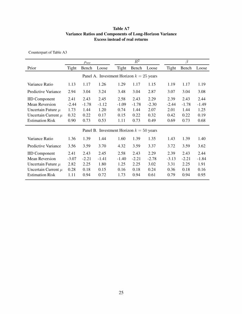
Table A7
Variance Ratios and Components of Long-Horizon Variance
Excess instead of real returns
Counterpart of Table A3
ρuw R2 β
Prior Tight Bench Loose Tight Bench Loose Tight Bench Loose
Panel A. Investment Horizon k = 25 years
Variance Ratio 1.13 1.17 1.26 1.29 1.17 1.15 1.19 1.17 1.19
Predictive Variance 2.94 3.04 3.24 3.48 3.04 2.87 3.07 3.04 3.08
IID Component 2.41 2.43 2.45 2.58 2.43 2.29 2.39 2.43 2.44
Mean Reversion -2.44 -1.78 -1.12 -1.09 -1.78 -2.30 -2.44 -1.78 -1.49
Uncertain Future µ 1.73 1.44 1.20 0.74 1.44 2.07 2.01 1.44 1.25
Uncertain Current µ 0.32 0.22 0.17 0.15 0.22 0.32 0.42 0.22 0.19
Estimation Risk 0.90 0.73 0.53 1.11 0.73 0.49 0.69 0.73 0.68
Panel B. Investment Horizon k = 50 years
Variance Ratio 1.36 1.39 1.44 1.60 1.39 1.35 1.43 1.39 1.40
Predictive Variance 3.56 3.59 3.70 4.32 3.59 3.37 3.72 3.59 3.62
IID Component 2.41 2.43 2.45 2.58 2.43 2.29 2.39 2.43 2.44
Mean Reversion -3.07 -2.21 -1.41 -1.40 -2.21 -2.78 -3.13 -2.21 -1.84
Uncertain Future µ 2.82 2.25 1.80 1.25 2.25 3.02 3.31 2.25 1.91
Uncertain Current µ 0.28 0.18 0.15 0.16 0.18 0.24 0.36 0.18 0.16
Estimation Risk 1.11 0.94 0.72 1.73 0.94 0.61 0.79 0.94 0.95
25
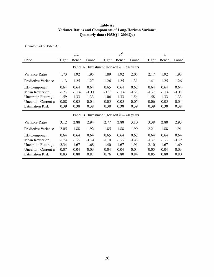
Table A8
Variance Ratios and Components of Long-Horizon Variance
Quarterly data (1952Q1–2006Q4)
Counterpart of Table A3
ρuw R2 β
Prior Tight Bench Loose Tight Bench Loose Tight Bench Loose
Panel A. Investment Horizon k = 25 years
Variance Ratio 1.73 1.92 1.95 1.89 1.92 2.05 2.17 1.92 1.93
Predictive Variance 1.13 1.25 1.27 1.26 1.25 1.31 1.41 1.25 1.26
IID Component 0.64 0.64 0.64 0.65 0.64 0.62 0.64 0.64 0.64
Mean Reversion -1.57 -1.14 -1.11 -0.88 -1.14 -1.29 -1.26 -1.14 -1.12
Uncertain Future µ 1.59 1.33 1.33 1.06 1.33 1.54 1.58 1.33 1.33
Uncertain Current µ 0.08 0.05 0.04 0.05 0.05 0.05 0.06 0.05 0.04
Estimation Risk 0.39 0.38 0.38 0.38 0.38 0.39 0.39 0.38 0.38
Panel B. Investment Horizon k = 50 years
Variance Ratio 3.12 2.88 2.94 2.77 2.88 3.10 3.38 2.88 2.93
Predictive Variance 2.05 1.88 1.92 1.85 1.88 1.99 2.21 1.88 1.91
IID Component 0.64 0.64 0.64 0.65 0.64 0.62 0.64 0.64 0.64
Mean Reversion -1.84 -1.27 -1.24 -1.01 -1.27 -1.42 -1.43 -1.27 -1.25
Uncertain Future µ 2.34 1.67 1.68 1.40 1.67 1.91 2.10 1.67 1.69
Uncertain Current µ 0.07 0.04 0.03 0.04 0.04 0.04 0.05 0.04 0.03
Estimation Risk 0.83 0.80 0.81 0.76 0.80 0.84 0.85 0.80 0.80
26

Table A9
Variance Ratios and Components of Long-Horizon Variance
Quarterly data (1952Q1–2006Q4)
One predictor instead of three (dividend yield)
Counterpart of Table A3
ρuw R2 β
Prior Tight Bench Loose Tight Bench Loose Tight Bench Loose
Panel A. Investment Horizon k = 25 years
Variance Ratio 3.54 2.20 2.30 1.97 2.20 2.24 2.67 2.20 2.15
Predictive Variance 2.36 1.50 1.57 1.36 1.50 1.51 1.82 1.50 1.47
IID Component 0.64 0.66 0.67 0.67 0.66 0.65 0.66 0.66 0.66
Mean Reversion -2.04 -0.76 -0.55 -0.79 -0.76 -0.73 -0.90 -0.76 -0.75
Uncertain Future µ 2.98 1.16 1.06 1.01 1.16 1.18 1.54 1.16 1.13
Uncertain Current µ 0.40 0.12 0.11 0.15 0.12 0.10 0.18 0.12 0.11
Estimation Risk 0.38 0.31 0.29 0.31 0.31 0.31 0.33 0.31 0.31
Panel B. Investment Horizon k = 50 years
Variance Ratio 8.07 3.48 3.49 3.33 3.48 3.36 4.46 3.48 3.37
Predictive Variance 5.38 2.37 2.39 2.29 2.37 2.27 3.04 2.37 2.30
IID Component 0.64 0.66 0.67 0.67 0.66 0.65 0.66 0.66 0.66
Mean Reversion -2.76 -0.90 -0.65 -0.99 -0.90 -0.83 -1.09 -0.90 -0.88
Uncertain Future µ 6.19 1.80 1.62 1.78 1.80 1.67 2.53 1.80 1.73
Uncertain Current µ 0.42 0.11 0.09 0.15 0.11 0.08 0.16 0.11 0.09
Estimation Risk 0.88 0.71 0.66 0.68 0.71 0.70 0.78 0.71 0.70
27
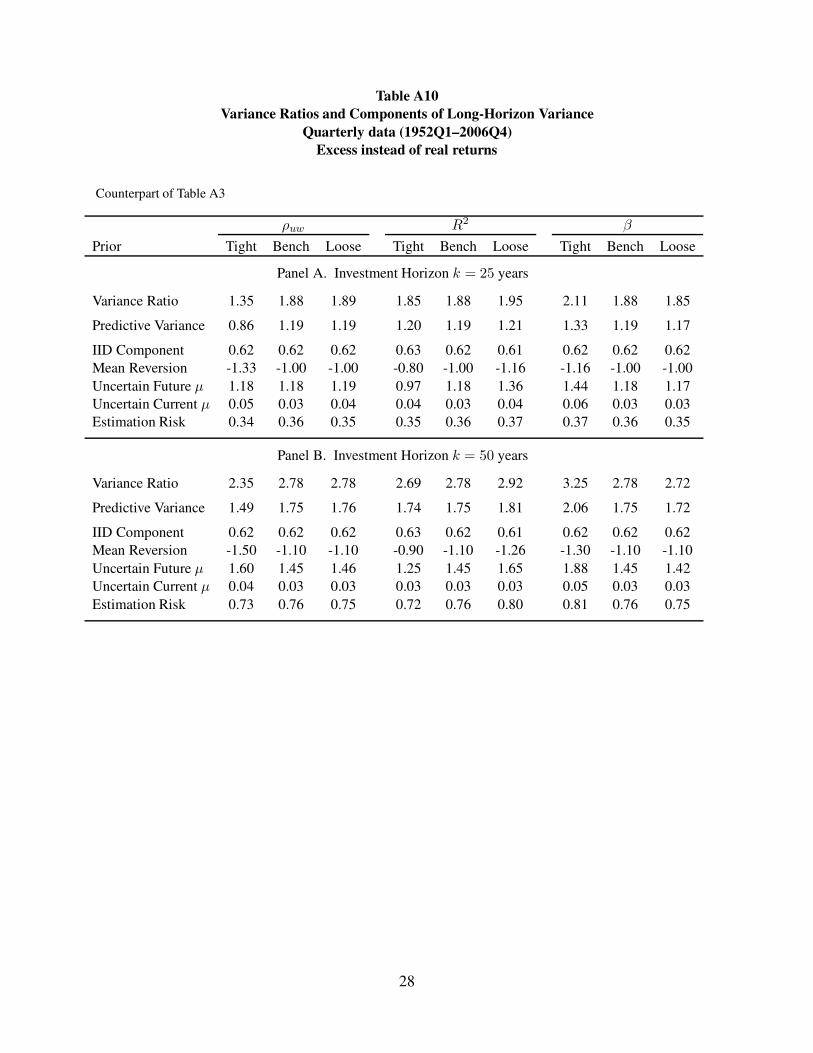
Table A10
Variance Ratios and Components of Long-Horizon Variance
Quarterly data (1952Q1–2006Q4)
Excess instead of real returns
Counterpart of Table A3
ρuw R2 β
Prior Tight Bench Loose Tight Bench Loose Tight Bench Loose
Panel A. Investment Horizon k = 25 years
Variance Ratio 1.35 1.88 1.89 1.85 1.88 1.95 2.11 1.88 1.85
Predictive Variance 0.86 1.19 1.19 1.20 1.19 1.21 1.33 1.19 1.17
IID Component 0.62 0.62 0.62 0.63 0.62 0.61 0.62 0.62 0.62
Mean Reversion -1.33 -1.00 -1.00 -0.80 -1.00 -1.16 -1.16 -1.00 -1.00
Uncertain Future µ 1.18 1.18 1.19 0.97 1.18 1.36 1.44 1.18 1.17
Uncertain Current µ 0.05 0.03 0.04 0.04 0.03 0.04 0.06 0.03 0.03
Estimation Risk 0.34 0.36 0.35 0.35 0.36 0.37 0.37 0.36 0.35
Panel B. Investment Horizon k = 50 years
Variance Ratio 2.35 2.78 2.78 2.69 2.78 2.92 3.25 2.78 2.72
Predictive Variance 1.49 1.75 1.76 1.74 1.75 1.81 2.06 1.75 1.72
IID Component 0.62 0.62 0.62 0.63 0.62 0.61 0.62 0.62 0.62
Mean Reversion -1.50 -1.10 -1.10 -0.90 -1.10 -1.26 -1.30 -1.10 -1.10
Uncertain Future µ 1.60 1.45 1.46 1.25 1.45 1.65 1.88 1.45 1.42
Uncertain Current µ 0.04 0.03 0.03 0.03 0.03 0.03 0.05 0.03 0.03
Estimation Risk 0.73 0.76 0.75 0.72 0.76 0.80 0.81 0.76 0.75
28
0 0.2 0.4 0.6 0.8 10
1
2
3
4
5
β0 0.2 0.4 0.6 0.8
0
2
4
6
8
10
R2
−1 −0.5 0 0.5 10
0.5
1
1.5
2
2.5
3
3.5
4
ρuw
0 0.2 0.4 0.6 0.8 10
0.5
1
1.5
2
2.5
ρµ b
Figure A1. Distributions for uncertain parameters The plots display the probability densities used to
illustrate the effects of parameter uncertainty on long-run variance. In the R2 panel, the solid line plots
the density of the true R2 (predictability given µT ), and the dashed line plots the implied density of the
R-squared in a regression of returns on bT . The dashed line incorporates the uncertainty about ρµb.
29
5 10 15 20 25 30 35 40 45 500.025
0.03
0.035
0.04
0.045
0.05
0.055
Predictive Horizon (years)
Va
ria
nce
(p
er
ye
ar)
Panel A. Predictive Variance of Stock Returns
5 10 15 20 25 30 35 40 45 50−0.06
−0.04
−0.02
0
0.02
0.04
0.06
Predictive Horizon (years)
Va
ria
nce
(p
er
ye
ar)
Panel B. Components of Predictive Variance
IID component
Mean reversion
Uncertain future µ
Uncertain current µ
Estimation risk
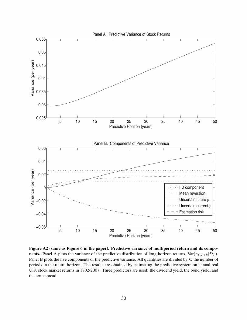
Figure A2 (same as Figure 6 in the paper). Predictive variance of multiperiod return and its compo-
nents. Panel A plots the variance of the predictive distribution of long-horizon returns, Var(rT,T+k|DT ).
Panel B plots the five components of the predictive variance. All quantities are divided by k, the number of
periods in the return horizon. The results are obtained by estimating the predictive system on annual real
U.S. stock market returns in 1802-2007. Three predictors are used: the dividend yield, the bond yield, and
the term spread.
30
5 10 15 20 25 30 35 40 45 500.025
0.03
0.035
0.04
0.045
0.05
0.055
0.06
Predictive Horizon (years)
Var
ianc
e (p
er y
ear)
Predictive Variance of Stock Returns: Different Priors
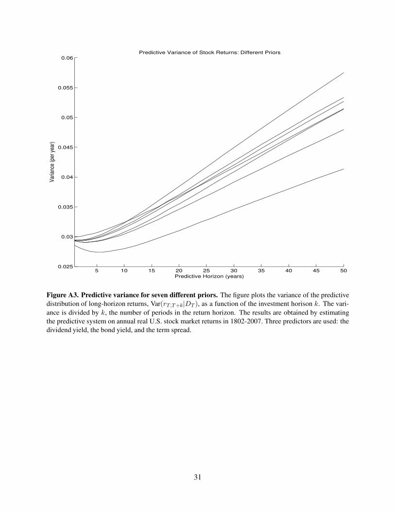
Figure A3. Predictive variance for seven different priors. The figure plots the variance of the predictive
distribution of long-horizon returns, Var(rT,T+k|DT ), as a function of the investment horison k. The vari-
ance is divided by k, the number of periods in the return horizon. The results are obtained by estimating
the predictive system on annual real U.S. stock market returns in 1802-2007. Three predictors are used: the
dividend yield, the bond yield, and the term spread.
31
5 10 15 20 25 30 35 40 45 500.02
0.025
0.03
0.035
0.04
Predictive Horizon (years)
Va
ria
nce
(p
er
ye
ar)
Panel A. Predictive Variance of Stock Returns
5 10 15 20 25 30 35 40 45 50−0.03
−0.02
−0.01
0
0.01
0.02
0.03
Predictive Horizon (years)
Va
ria
nce
(p
er
ye
ar)
Panel B. Components of Predictive Variance
IID component
Mean reversion
Uncertain future µ
Uncertain current µ
Estimation risk
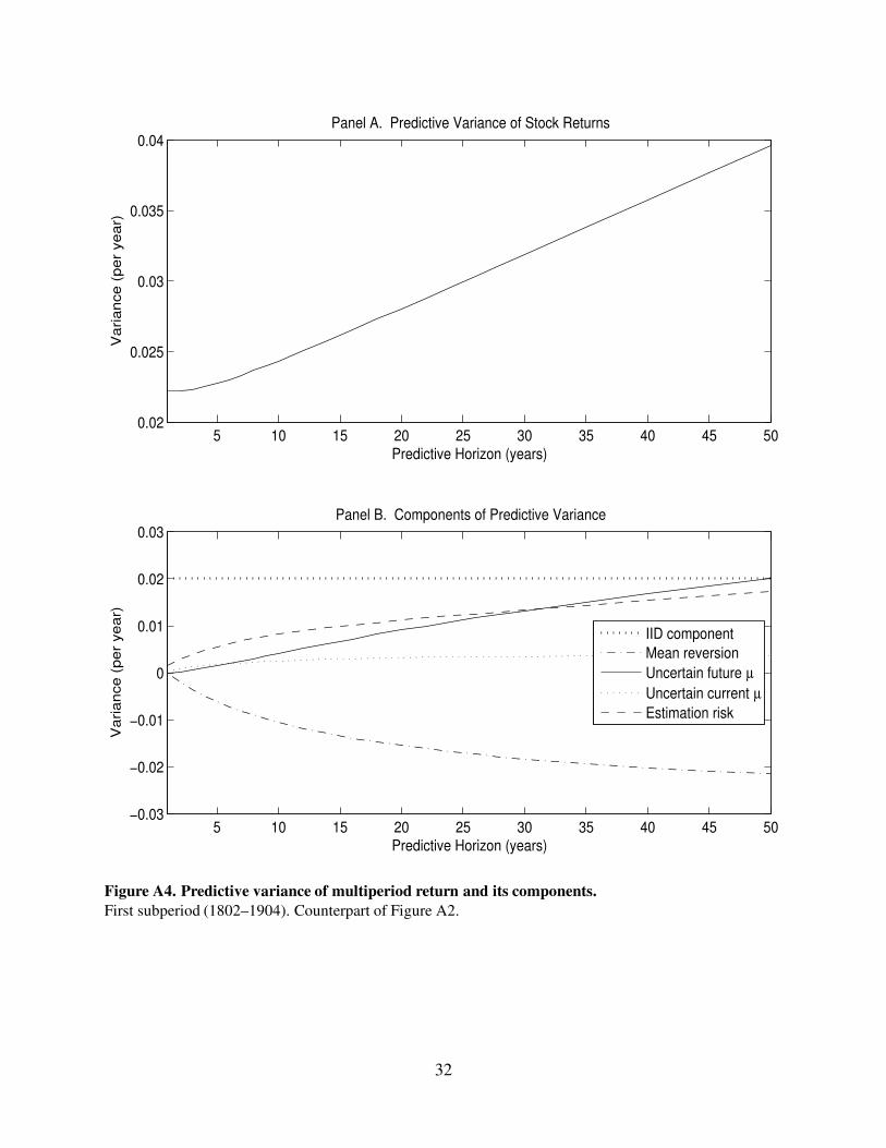
Figure A4. Predictive variance of multiperiod return and its components.
First subperiod (1802–1904). Counterpart of Figure A2.
32
5 10 15 20 25 30 35 40 45 500.02
0.025
0.03
0.035
0.04
0.045
0.05
Predictive Horizon (years)
Var
ianc
e (p
er y
ear)
Predictive Variance of Stock Returns: Different Priors
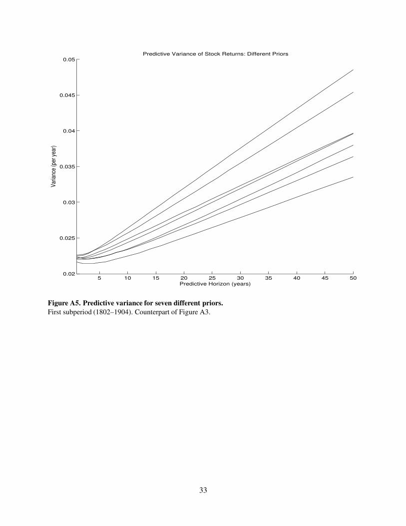
Figure A5. Predictive variance for seven different priors.
First subperiod (1802–1904). Counterpart of Figure A3.
33
5 10 15 20 25 30 35 40 45 500.03
0.035
0.04
0.045
0.05
0.055
Predictive Horizon (years)
Va
ria
nce
(p
er
ye
ar)
Panel A. Predictive Variance of Stock Returns
5 10 15 20 25 30 35 40 45 50−0.06
−0.04
−0.02
0
0.02
0.04
0.06
Predictive Horizon (years)
Va
ria
nce
(p
er
ye
ar)
Panel B. Components of Predictive Variance
IID component
Mean reversion
Uncertain future µ
Uncertain current µ
Estimation risk
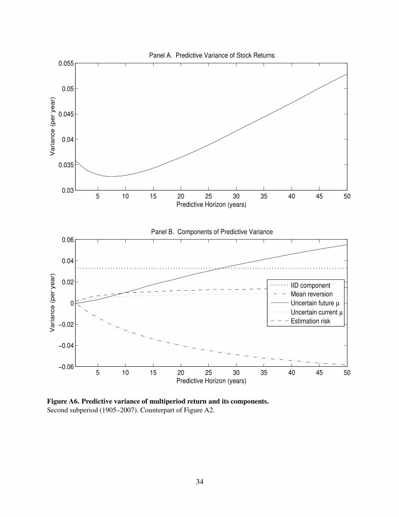
Figure A6. Predictive variance of multiperiod return and its components.
Second subperiod (1905–2007). Counterpart of Figure A2.
34
5 10 15 20 25 30 35 40 45 500.03
0.035
0.04
0.045
0.05
0.055
0.06
0.065
0.07
0.075
Predictive Horizon (years)
Var
ianc
e (p
er y
ear)
Predictive Variance of Stock Returns: Different Priors
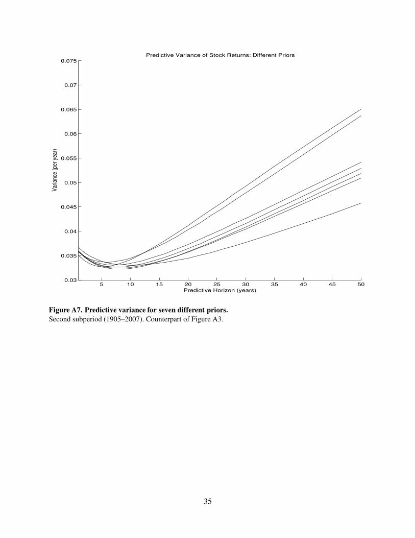
Figure A7. Predictive variance for seven different priors.
Second subperiod (1905–2007). Counterpart of Figure A3.
35
5 10 15 20 25 30 35 40 45 500.026
0.028
0.03
0.032
0.034
0.036
0.038
0.04
Predictive Horizon (years)
Va
ria
nce
(p
er
ye
ar)
Panel A. Predictive Variance of Stock Returns
5 10 15 20 25 30 35 40 45 50−0.06
−0.04
−0.02
0
0.02
0.04
Predictive Horizon (years)
Va
ria
nce
(p
er
ye
ar)
Panel B. Components of Predictive Variance
IID component
Mean reversion
Uncertain future µ
Uncertain current µ
Estimation risk
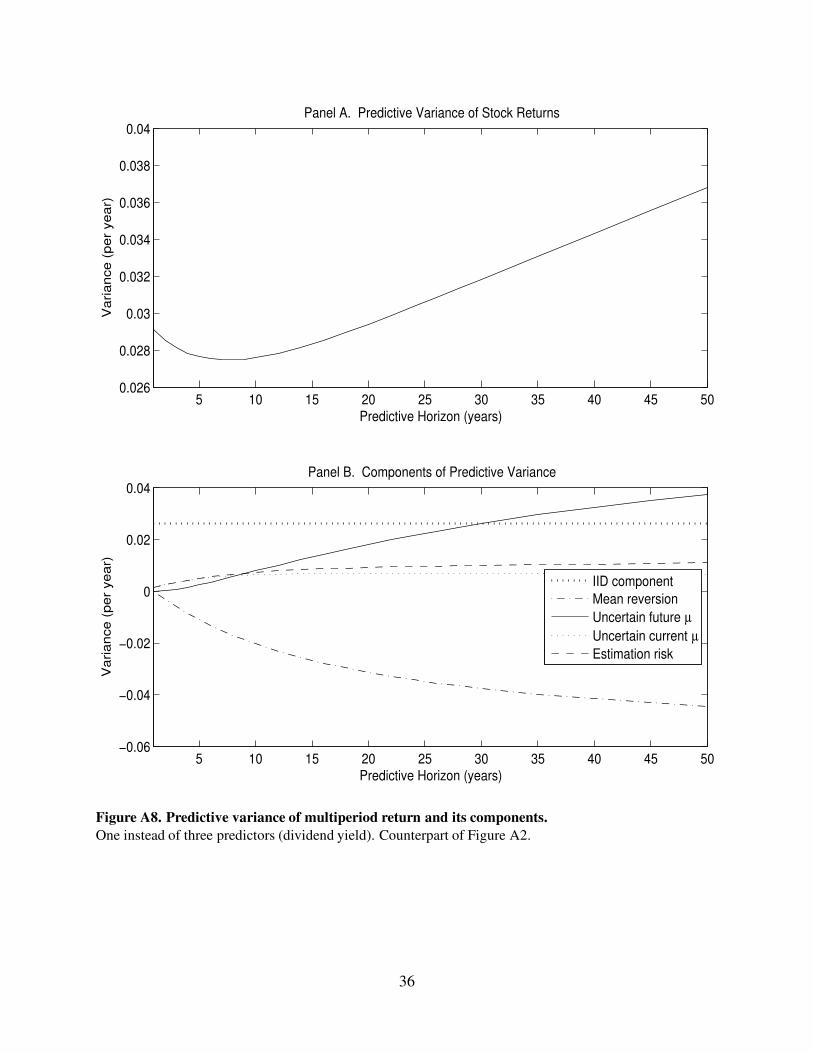
Figure A8. Predictive variance of multiperiod return and its components.
One instead of three predictors (dividend yield). Counterpart of Figure A2.
36
5 10 15 20 25 30 35 40 45 500.024
0.026
0.028
0.03
0.032
0.034
0.036
0.038
0.04
0.042
0.044
Predictive Horizon (years)
Var
ianc
e (p
er y
ear)
Predictive Variance of Stock Returns: Different Priors
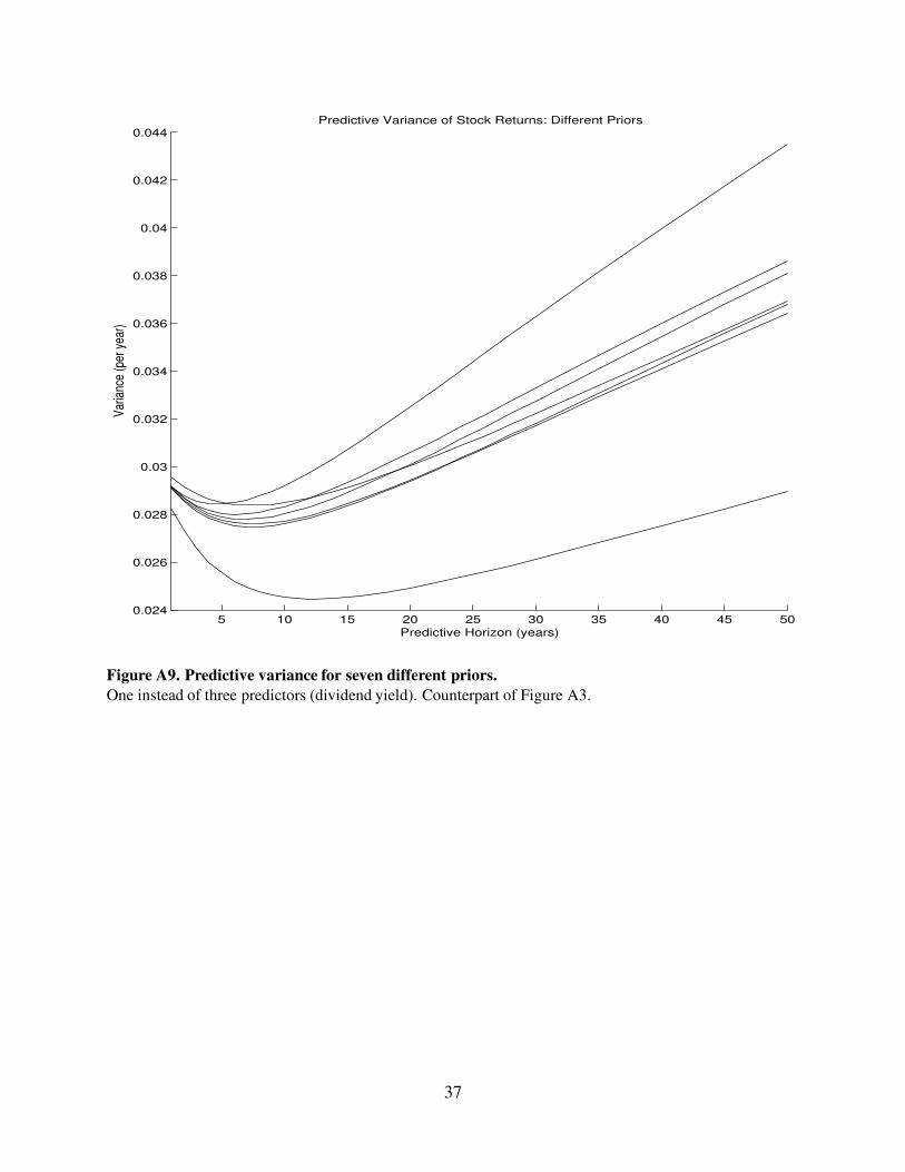
Figure A9. Predictive variance for seven different priors.
One instead of three predictors (dividend yield). Counterpart of Figure A3.
37
5 10 15 20 25 30 35 40 45 500.024
0.026
0.028
0.03
0.032
0.034
0.036
0.038
Predictive Horizon (years)
Va
ria
nce
(p
er
ye
ar)
Panel A. Predictive Variance of Stock Returns
5 10 15 20 25 30 35 40 45 50−0.03
−0.02
−0.01
0
0.01
0.02
0.03
Predictive Horizon (years)
Va
ria
nce
(p
er
ye
ar)
Panel B. Components of Predictive Variance
IID component
Mean reversion
Uncertain future µ
Uncertain current µ
Estimation risk
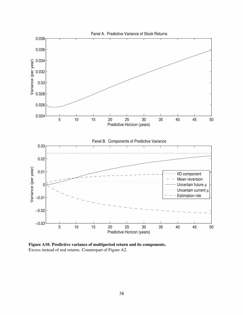
Figure A10. Predictive variance of multiperiod return and its components.
Excess instead of real returns. Counterpart of Figure A2.
38
5 10 15 20 25 30 35 40 45 500.024
0.026
0.028
0.03
0.032
0.034
0.036
0.038
0.04
0.042
0.044
Predictive Horizon (years)
Var
ianc
e (p
er y
ear)
Predictive Variance of Stock Returns: Different Priors
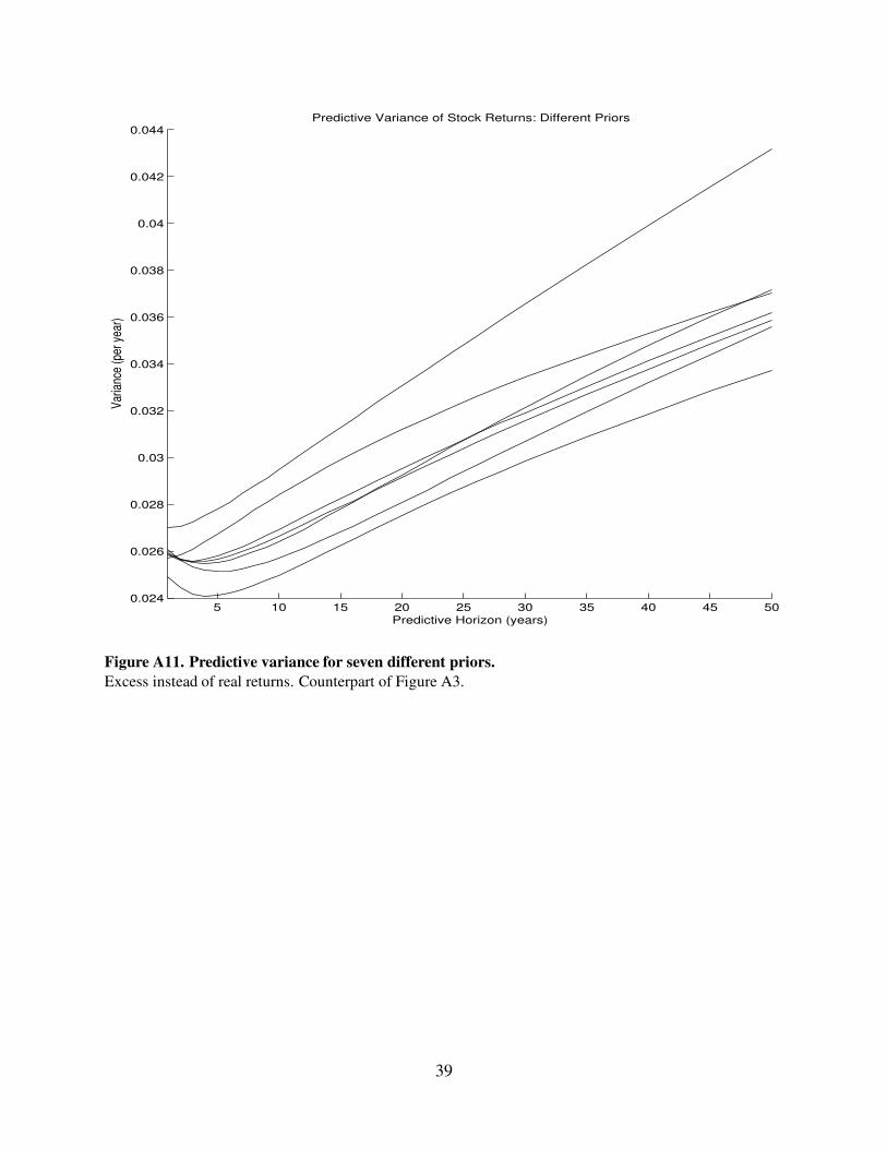
Figure A11. Predictive variance for seven different priors.
Excess instead of real returns. Counterpart of Figure A3.
39
10 20 30 40 50 60 70 80 90 100 110 1200.005
0.01
0.015
Predictive Horizon (quarters)
Va
ria
nce
(p
er
qu
art
er)
Panel A. Predictive Variance of Stock Returns
10 20 30 40 50 60 70 80 90 100 110 120−0.015
−0.01
−0.005
0
0.005
0.01
0.015
Predictive Horizon (quarters)
Va
ria
nce
(p
er
qu
art
er)
Panel B. Components of Predictive Variance
IID component
Mean reversion
Uncertain future µ
Uncertain current µ
Estimation risk
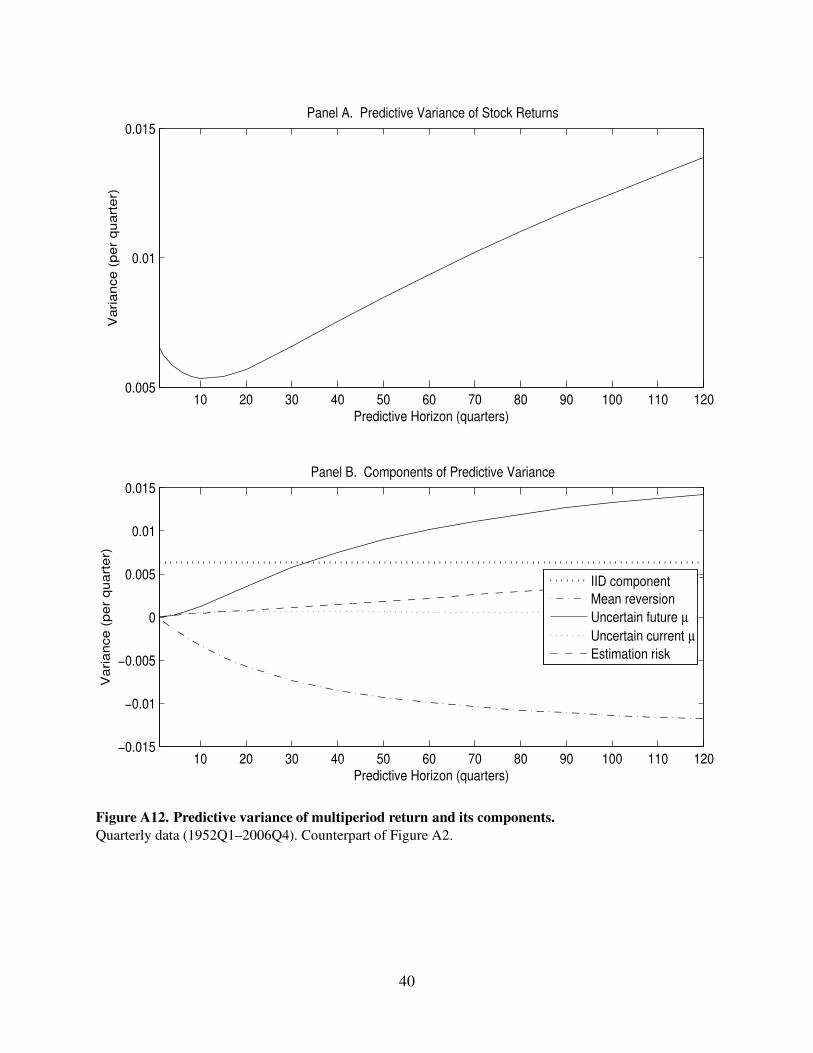
Figure A12. Predictive variance of multiperiod return and its components.
Quarterly data (1952Q1–2006Q4). Counterpart of Figure A2.
40
20 40 60 80 100 120 140 160 180 2000.004
0.006
0.008
0.01
0.012
0.014
0.016
0.018
0.02
0.022
0.024
Predictive Horizon (quarters)
Var
ianc
e (p
er q
uart
er)
Predictive Variance of Stock Returns: Different Priors
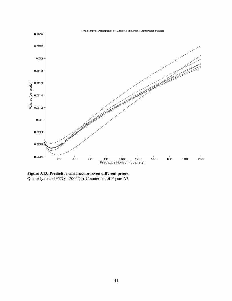
Figure A13. Predictive variance for seven different priors.
Quarterly data (1952Q1–2006Q4). Counterpart of Figure A3.
41
10 20 30 40 50 60 70 80 90 100 110 1200.006
0.008
0.01
0.012
0.014
0.016
0.018
0.02
Predictive Horizon (quarters)
Va
ria
nce
(p
er
qu
art
er)
Panel A. Predictive Variance of Stock Returns
10 20 30 40 50 60 70 80 90 100 110 120−0.01
−0.005
0
0.005
0.01
0.015
Predictive Horizon (quarters)
Va
ria
nce
(p
er
qu
art
er)
Panel B. Components of Predictive Variance
IID component
Mean reversion
Uncertain future µ
Uncertain current µ
Estimation risk
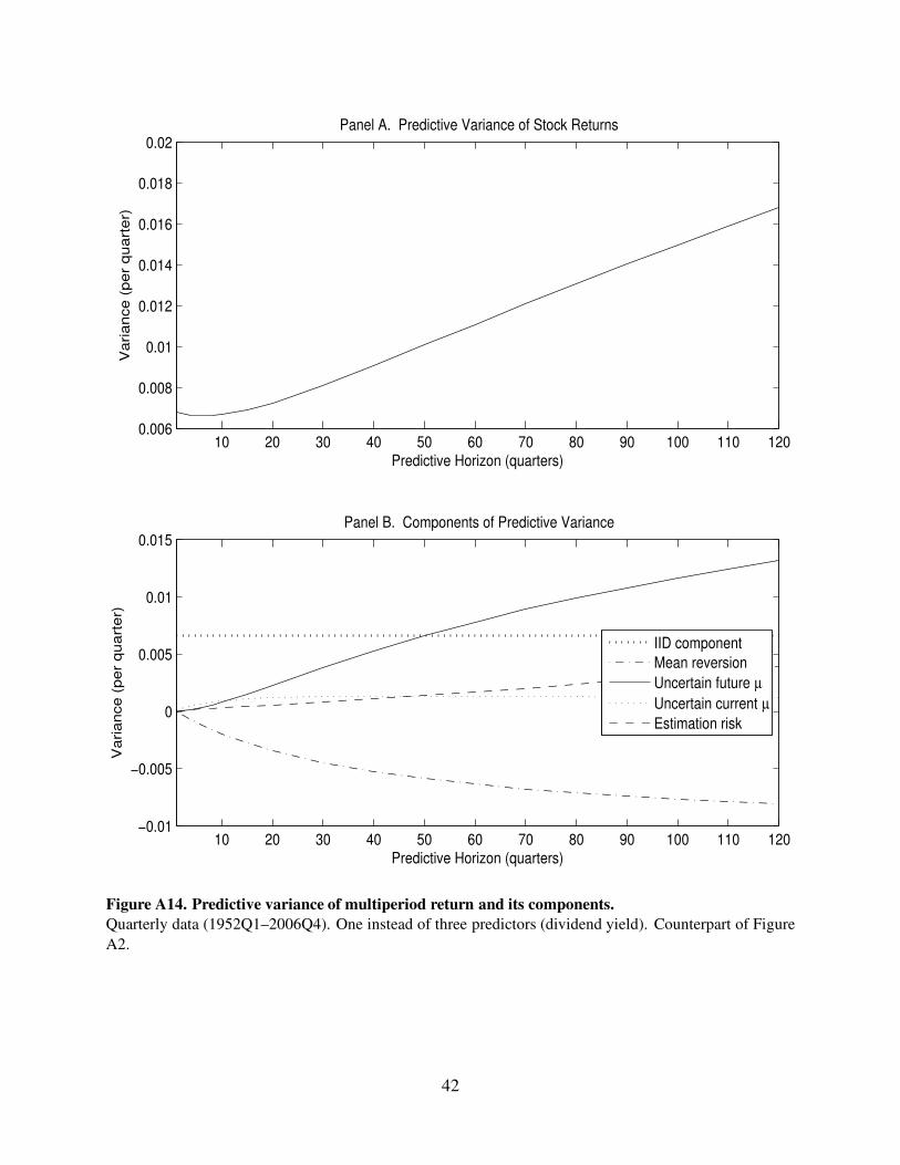
Figure A14. Predictive variance of multiperiod return and its components.
Quarterly data (1952Q1–2006Q4). One instead of three predictors (dividend yield). Counterpart of Figure
A2.
42
20 40 60 80 100 120 140 160 180 2000.005
0.01
0.015
0.02
0.025
0.03
0.035
0.04
0.045
0.05
0.055
Predictive Horizon (quarters)
Var
ianc
e (p
er q
uart
er)
Predictive Variance of Stock Returns: Different Priors
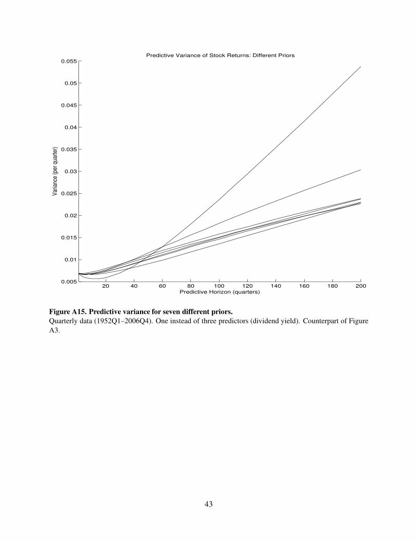
Figure A15. Predictive variance for seven different priors.
Quarterly data (1952Q1–2006Q4). One instead of three predictors (dividend yield). Counterpart of Figure
A3.
43
10 20 30 40 50 60 70 80 90 100 110 1200.005
0.01
0.015
Predictive Horizon (quarters)
Va
ria
nce
(p
er
qu
art
er)
Panel A. Predictive Variance of Stock Returns
10 20 30 40 50 60 70 80 90 100 110 120−0.015
−0.01
−0.005
0
0.005
0.01
0.015
Predictive Horizon (quarters)
Va
ria
nce
(p
er
qu
art
er)
Panel B. Components of Predictive Variance
IID component
Mean reversion
Uncertain future µ
Uncertain current µ
Estimation risk
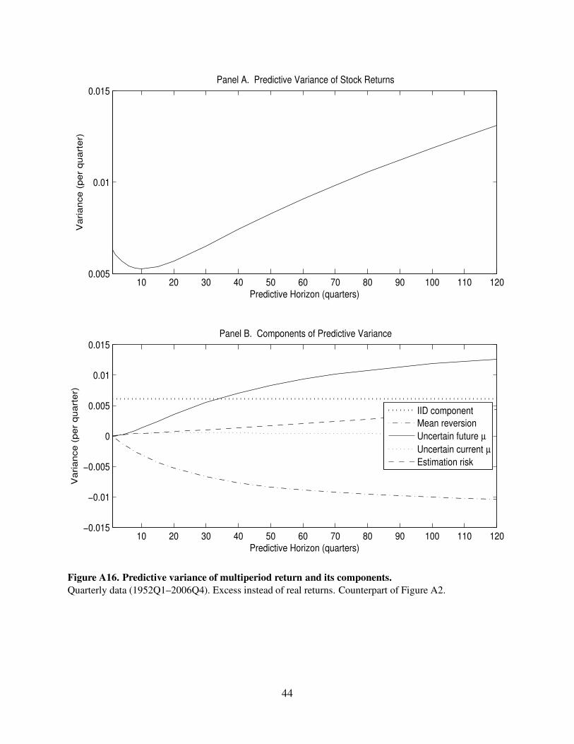
Figure A16. Predictive variance of multiperiod return and its components.
Quarterly data (1952Q1–2006Q4). Excess instead of real returns. Counterpart of Figure A2.
44
20 40 60 80 100 120 140 160 180 2000.002
0.004
0.006
0.008
0.01
0.012
0.014
0.016
0.018
0.02
0.022
Predictive Horizon (quarters)
Var
ianc
e (p
er q
uart
er)
Predictive Variance of Stock Returns: Different Priors
Figure A17. Predictive variance for seven different priors.
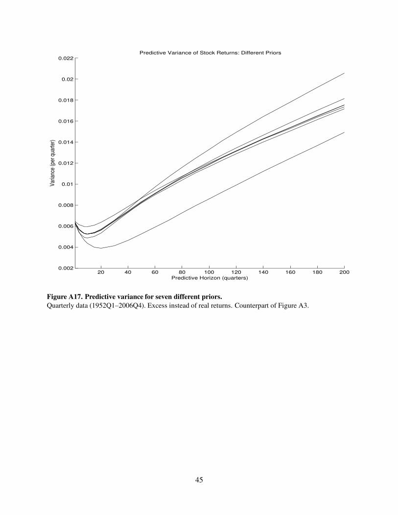
Quarterly data (1952Q1–2006Q4). Excess instead of real returns. Counterpart of Figure A3.
45
0 0.02 0.04 0.06 0.08 0.10
0.2
0.4
0.6
0.8
1
σπ
Density (
rescale
d)
A. Prior for Standard Deviation of π
0 0.01 0.02 0.03 0.04 0.050
0.2
0.4
0.6
0.8
1
∆ R2
Density (
rescale
d)
C. Posterior for Increase in R2
10 20 30 40 500.030
0.035
0.040
0.045
Horizon (years)
Variance (
per
year)
E. Predictive Variance of Returns
0 0.02 0.04 0.06 0.08 0.10
0.2
0.4
0.6
0.8
1
σπ
Density (
rescale
d)
B. Prior for Standard Deviation of π
0 0.01 0.02 0.03 0.04 0.050
0.2
0.4
0.6
0.8
1
∆ R2
Density (
rescale
d)
D. Posterior for Increase in R2
50 100 150 2000.003
0.006
0.009
0.012
Horizon (quarters)
Variance (
per
quart
er)
F. Predictive Variance of Returns
less imperfect
more imperfect
perfect (σπ=0)
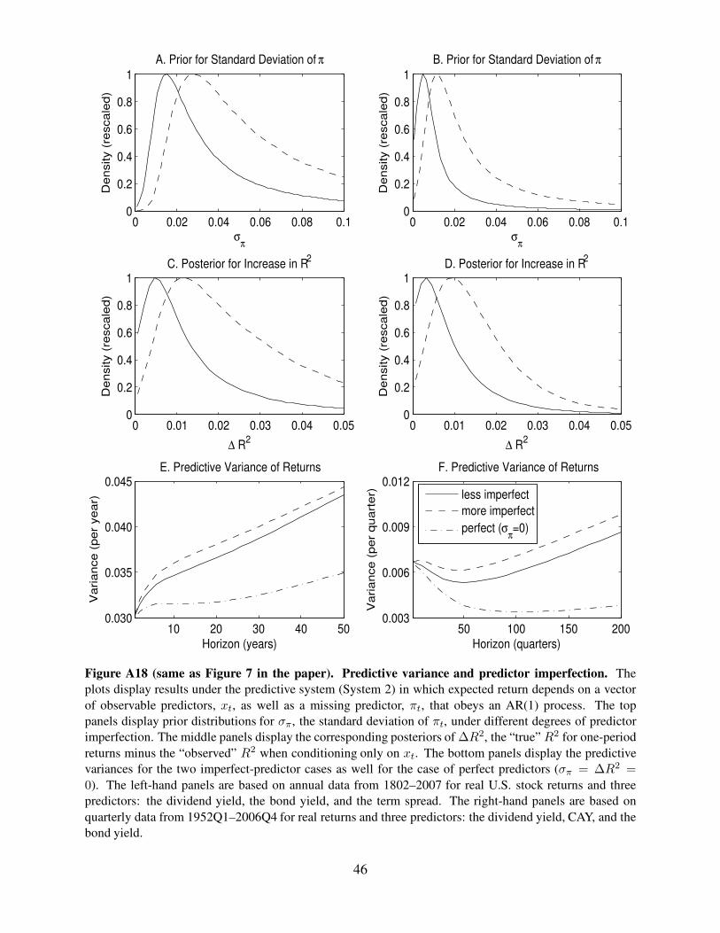
Figure A18 (same as Figure 7 in the paper). Predictive variance and predictor imperfection. The
plots display results under the predictive system (System 2) in which expected return depends on a vector
of observable predictors, xt, as well as a missing predictor, πt, that obeys an AR(1) process. The top
panels display prior distributions for σπ, the standard deviation of πt, under different degrees of predictor
imperfection. The middle panels display the corresponding posteriors of ∆R2, the “true” R2 for one-period
returns minus the “observed” R2 when conditioning only on xt. The bottom panels display the predictive
variances for the two imperfect-predictor cases as well for the case of perfect predictors (σπ = ∆R2 =
0). The left-hand panels are based on annual data from 1802–2007 for real U.S. stock returns and three
predictors: the dividend yield, the bond yield, and the term spread. The right-hand panels are based on
quarterly data from 1952Q1–2006Q4 for real returns and three predictors: the dividend yield, CAY, and the
bond yield.
46
0 0.02 0.04 0.06 0.08 0.10
0.2
0.4
0.6
0.8
1
σπ
De
nsity (
resca
led
)
A. Prior for Standard Deviation of π
0 0.02 0.04 0.06 0.08 0.10
0.2
0.4
0.6
0.8
1
∆ R2
De
nsity (
resca
led
)
C. Posterior for Increase in R2
10 20 30 40 50
0.04
0.06
0.08
0.1
Horizon (years)
Va
ria
nce
(p
er
ye
ar)
E. Predictive Variance of Returns
0 0.02 0.04 0.06 0.08 0.10
0.2
0.4
0.6
0.8
1
σπ
De
nsity (
resca
led
)
B. Prior for Standard Deviation of π
0 0.02 0.04 0.06 0.08 0.10
0.2
0.4
0.6
0.8
1
∆ R2
De
nsity (
resca
led
)
D. Posterior for Increase in R2
10 20 30 40 500.04
0.06
0.08
0.1
Horizon (years)
Va
ria
nce
(p
er
ye
ar)
F. Predictive Variance of Returns
less imperfect
more imperfect
perfect (σπ=0)
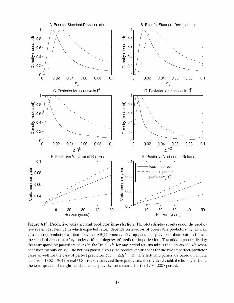
Figure A19. Predictive variance and predictor imperfection. The plots display results under the predic-
tive system (System 2) in which expected return depends on a vector of observable predictors, xt, as well
as a missing predictor, πt, that obeys an AR(1) process. The top panels display prior distributions for σπ ,
the standard deviation of πt, under different degrees of predictor imperfection. The middle panels display
the corresponding posteriors of ∆R2, the “true” R2 for one-period returns minus the “observed” R2 when
conditioning only on xt. The bottom panels display the predictive variances for the two imperfect-predictor
cases as well for the case of perfect predictors (σπ = ∆R2 = 0). The left-hand panels are based on annual
data from 1802–1904 for real U.S. stock returns and three predictors: the dividend yield, the bond yield, and
the term spread. The right-hand panels display the same results for the 1905–2007 period.
47
0 0.02 0.04 0.06 0.08 0.10
0.2
0.4
0.6
0.8
1
σπ
De
nsity (
resca
led
)
A. Prior for Standard Deviation of π
0 0.01 0.02 0.03 0.04 0.050
0.2
0.4
0.6
0.8
1
∆ R2
De
nsity (
resca
led
)
C. Posterior for Increase in R2
10 20 30 40 50
0.030
0.035
0.040
Horizon (years)
Va
ria
nce
(p
er
ye
ar)
E. Predictive Variance of Returns
0 0.02 0.04 0.06 0.08 0.10
0.2
0.4
0.6
0.8
1
σπ
De
nsity (
resca
led
)
B. Prior for Standard Deviation of π
0 0.01 0.02 0.03 0.04 0.050
0.2
0.4
0.6
0.8
1
∆ R2
De
nsity (
resca
led
)
D. Posterior for Increase in R2
50 100 150 2000.003
0.006
0.009
0.012
Horizon (quarters)
Va
ria
nce
(p
er
qu
art
er)
F. Predictive Variance of Returns
less imperfect
more imperfect
perfect (σπ=0)
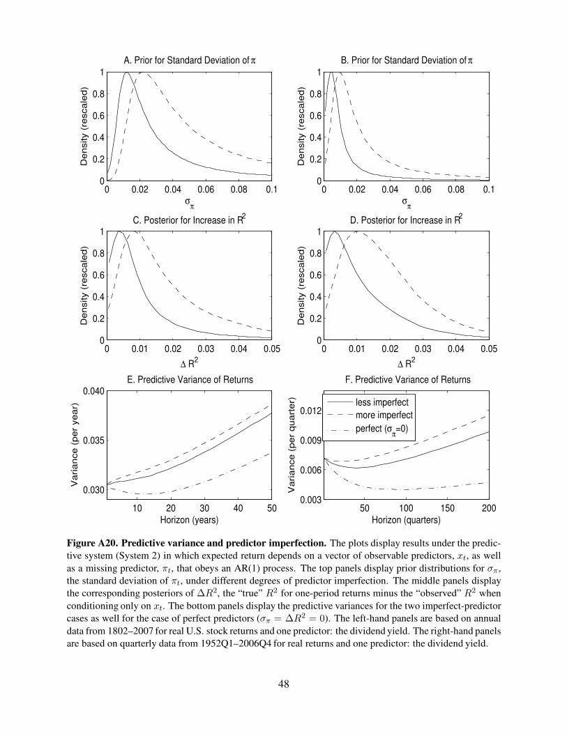
Figure A20. Predictive variance and predictor imperfection. The plots display results under the predic-
tive system (System 2) in which expected return depends on a vector of observable predictors, xt, as well
as a missing predictor, πt, that obeys an AR(1) process. The top panels display prior distributions for σπ ,
the standard deviation of πt, under different degrees of predictor imperfection. The middle panels display
the corresponding posteriors of ∆R2, the “true” R2 for one-period returns minus the “observed” R2 when
conditioning only on xt. The bottom panels display the predictive variances for the two imperfect-predictor
cases as well for the case of perfect predictors (σπ = ∆R2 = 0). The left-hand panels are based on annual
data from 1802–2007 for real U.S. stock returns and one predictor: the dividend yield. The right-hand panels
are based on quarterly data from 1952Q1–2006Q4 for real returns and one predictor: the dividend yield.
48

0 0.02 0.04 0.06 0.08 0.10
0.2
0.4
0.6
0.8
1
σπ
De
nsity (
resca
led
)
A. Prior for Standard Deviation of π
0 0.01 0.02 0.03 0.04 0.050
0.2
0.4
0.6
0.8
1
∆ R2
De
nsity (
resca
led
)
C. Posterior for Increase in R2
10 20 30 40 50
0.030
0.035
0.040
0.045
Horizon (years)
Va
ria
nce
(p
er
ye
ar)
E. Predictive Variance of Returns
0 0.02 0.04 0.06 0.08 0.10
0.2
0.4
0.6
0.8
1
σπ
De
nsity (
resca
led
)
B. Prior for Standard Deviation of π
0 0.01 0.02 0.03 0.04 0.050
0.2
0.4
0.6
0.8
1
∆ R2
De
nsity (
resca
led
)
D. Posterior for Increase in R2
50 100 150 2000.003
0.006
0.009
0.012
Horizon (quarters)
Va
ria
nce
(p
er
qu
art
er)
F. Predictive Variance of Returns
less imperfect
more imperfect
perfect (σπ=0)
Figure A21. Predictive variance and predictor imperfection. The plots display results under the predic-
tive system (System 2) in which expected return depends on a vector of observable predictors, xt, as well
as a missing predictor, πt, that obeys an AR(1) process. The top panels display prior distributions for σπ ,
the standard deviation of πt, under different degrees of predictor imperfection. The middle panels display
the corresponding posteriors of ∆R2, the “true” R2 for one-period returns minus the “observed” R2 when
conditioning only on xt. The bottom panels display the predictive variances for the two imperfect-predictor
cases as well for the case of perfect predictors (σπ = ∆R2 = 0). The left-hand panels are based on annual
data from 1802–2007 for excess U.S. stock returns and three predictors: the dividend yield, the bond yield,
and the term spread. The right-hand panels are based on quarterly data from 1952Q1–2006Q4 for excess
returns and three predictors: the dividend yield, CAY, and the bond yield.
49

References
Carter, Chris K., and Robert Kohn, 1994, On Gibbs sampling for state space models, Biometrika 81, 541–
553.
Fruhwirth-Schnatter, Sylvia, 1994, Data augmentation and dynamic linear models, Journal of Time Series
Analysis 15, 183–202.
Stambaugh, Robert F., 1997, Analyzing investments whose histories differ in length, Journal of Financial
Economics 45, 285–331.
West, Mike, and Jeff Harrison, 1997, Bayesian Forecasting and Dynamic Models (Springer-Verlag, New
York, NY).
Zellner, Arnold, 1971, An Introduction to Bayesian Inference in Econometrics (John Wiley & Sons, New
York, NY).
50