International Correlation Risk∗

Philippe MuellerLondon School of Economics

Andreas StathopoulosUSC Marshall School of Business

Andrea VedolinLondon School of Economics

Abstract

In this paper, we find that FX correlation is a key driver of FX risk premia and carry trade

returns. We show that the correlation risk premium, defined as the difference between

the risk-neutral and objective measure correlation is large (15% per year) and highly

time-varying. Sorting currencies according to their exposure with correlation innovations

yields portfolios with attractive risk and return characteristics. Moreover, high (low)

interest rate currencies have negative (positive) loadings on the correlation risk factor. To

address our empirical findings, we consider a multi-country general equilibrium model with

time-varying risk aversion generated by external habit preferences. In the model, currency

risk premia compensate for exposure to global risk aversion, defined as a weighted average

of country risk aversions. We show that high global risk aversion is associated with high

conditional exchange rate second moments, so currencies that hedge against adverse global

risk aversion fluctuations can be empirically identified as currencies that appreciate when

conditional exchange rate second moments are high. If the precautionary savings motive

is sufficiently strong, the model can also address the forward premium puzzle, as high

interest rate currencies are very exposed to global risk aversion increases (whereas low

interest rate currencies provide a hedge against such an increase).

JEL Classification Codes: F31, G12, G13.

Keywords: Carry Trade, Correlation Risk, Habit Formation, International Finance, Exchange Rates.

First Version: December 2011.

This Version: April 2012.

∗Philippe Mueller and Andrea Vedolin acknowledge financial support from STICERD at LSE. Wewould like to thank Joe Chen, Mike Chernov, Ivan Shaliastovich, Adrien Verdelhan and seminar par-ticipants of LUISS Guido Carli, Rome, University of Lund, University of Piraeus, University of Bern,Stockholm School of Economics, London School of Economics, Chicago Booth Finance Symposium2011, 6th End of Year Meeting of the Swiss Economists Abroad, Duke/UNC Asset Pricing Conferenceand the UCLA-USC Finance Day 2012 for thoughtful comments. We very much welcome comments, in-cluding references that we have inadvertently overlooked. Contact information: p.mueller@lse.ac.uk,astathop@marshall.usc.edu and a.vedolin@lse.ac.uk.

Recent research has established that a significant component of currency risk premia

constitutes compensation for exposure to global risk. Motivated by this result, in this

paper we provide economic underpinnings to this priced risk. First, we empirically

establish that foreign exchange (FX) correlation risk is priced in the cross-section of

currency returns. Then, we link FX correlation risk to global risk aversion using a

multi-country general equilibrium model featuring external habit formation.

To show that FX correlation risk is priced, we start by constructing the currency

correlation risk premium for each pair of exchange rates using a cross-section of currency

option prices and high frequency data on the underlying spot exchange rates. We find

that the size of the estimated correlation risk premium, defined as the difference between

the risk-neutral and the objective measure exchange rate correlation, is economically

large and comparable to the one documented in the equity options literature: The

average correlation risk premium is around 15% with an average implied correlation of

56% and an average realized correlation of 41%.1

We then proceed by quantifying the price of FX correlation risk using a portfo-

lio sorting approach, following the recent international finance literature (Lustig and

Verdelhan, 2007, Lustig, Roussanov, and Verdelhan, 2011; Menkhoff, Sarno, Schmeling,

and Schrimpf, 2011; and Burnside, 2011). To this end, we construct an FX correlation

risk factor, defined as a cross-sectional average of conditional exchange rate correlations,

and sort currencies into four portfolios according to their exposure to that factor at the

end of each month. Intuitively, if correlation risk is priced in currency markets, then

currencies with low FX correlation betas (i.e. currencies that comove weakly with FX

correlation) should yield higher returns, whereas low correlation risk currencies (i.e. cur-

rencies that appreciate strongly when FX correlation increases and, thus, hedge against

FX correlation risk) should yield lower returns. Our results confirm that intuition: We

show that investing in the portfolio with the highest relative correlation risk exposure

(i.e. the portfolio consisting of the currencies that have negative FX correlation betas

and, thus, depreciate when FX correlation increases) while shorting the portfolio with

1Driessen, Maenhout, and Vilkov (2009) estimate that the correlation risk premium on the S&P 500is approximately 18%, with an average realized correlation of 29% and an average implied correlationof 47%.

1

the lowest correlation risk exposure generates an average excess return between 3% (all

countries) and 5% (developed countries) with a Sharpe ratio of 0.36 and 0.5, respectively.

Next, we address the forward premium puzzle by showing that carry trade returns are

due to high exposure to the FX correlation risk factor. Following the Fama and MacBeth

(1973) two-step procedure, we estimate the price of the FX correlation factor at almost

-1% per annum. Furthermore, we show that that high (low) interest rate currencies have

negative (positive) FX correlation betas and, therefore, depreciate (appreciate) in bad

states of the world, when global risk aversion is high. As a result, high interest rate

currencies have positive risk premia, whereas low interest rate currencies have low or

negative risk premia.

To address our empirical findings, we explore the implications of time variation in

conditional risk aversion for currency risk premia. For that purpose, we consider a

multi-country, multi-good general equilibrium model in which preferences are character-

ized by external habit formation (Menzly, Santos and Veronesi, 2004) and home bias,

as in Stathopoulos (2011, 2012). In the model, currency risk premia compensate in-

vestors mainly for exposure to global risk aversion fluctuations: the price of the global

risk aversion risk factor is negative, so agents are willing to accept lower returns for

assets that have negative global risk aversion betas and, thus, provide a hedge against

increases in global risk aversion. We also show that global risk aversion tends to be

positively associated with conditional exchange rate second moments, so currencies that

hedge against adverse global risk aversion fluctuations can be empirically identified as

currencies that appreciate when conditional exchange rate second moments are high.

Finally, we show that our model is able to link currency risk premia to real interest rate

differentials and, thus, address the forward premium puzzle. If real interest rates are

procyclical, which is true if the precautionary savings motive is sufficiently strong, being

long a high interest rate currency and short a low interest rate currency (i.e. engaging

in the carry trade) entails holding a position with a negative global risk aversion beta

and, thus, high exposure to the global risk aversion factor. As a result, investors require

a high compensation in terms of expected return in order to engage in the carry trade.

2

Related Literature: This paper builds on the extant literature on the risk-return rela-

tionship of excess returns in currency markets. Lustig, Roussanov, and Verdelhan (2012)

identify two new risk factors: the average forward discount of the US dollar against de-

veloped market currencies and the return to the carry trade portfolio itself. They then

study the predictive content of these two factors and find that the average forward dis-

count is the best predictor of average currency excess returns even when controlling for

the forward discount. While Lustig, Roussanov, and Verdelhan (2012) focus on currency

portfolios, Verdelhan (2011) finds high R2 from regressions of individual currency risk

premia on the average dollar factor. Using quantile regressions, Cenedese, Sarno, and

Tsiakas (2012) find that higher (lower) average currency excess return variance (corre-

lation) leads to larger losses (gains) in the carry trade. The paper closest to ours is by

Menkhoff, Sarno, Schmeling, and Schrimpf (2011) who study whether currency excess

returns can be explained by a compensation for global currency volatility risk. They

find that high interest rate currencies are negatively related to innovations in global FX

volatility and thus deliver low returns in times of unexpectedly high volatility, when

low interest rate currencies provide a hedge by yielding positive returns. Della Corte,

Sarno, and Tsiakas (2011) study the predictive power of forward implied volatility for

spot volatility in foreign exchange markets. They find that the forward implied volatility

is a biased predictor that overestimates movements in future spot implied volatility.

Our paper is part of the recent literature that addresses the failure of the expecta-

tions hypothesis for exchange rates. Brunnermeier, Nagel, and Pedersen (2009), Farhi,

Fraiberger, Gabaix, Ranciere and Verdelhan (2009), Jurek (2009), Burnside, Eichen-

baum, Kleshchelski and Rebelo (2011) and Farhi and Gabaix (2011) emphasize the im-

portance of disaster risk for currency risk premia, Yu (2011) studies the effect of investor

sentiment, while Colacito and Croce (2009, 2010) and Bansal and Shaliastovich (2011)

explore the implications of long-run risk in currency markets. Martin (2011) studies

the failure of the UIP in a two country economy with two goods and heterogeneity in

country size. The paper closest to ours is Verdelhan (2010): he proposes a two-country,

single-good model with trade frictions and time-varying risk aversion generated by ex-

ternal habit formation and illustrates the importance of procyclical real interest rates

3

for addressing the forward premium puzzle. In our multi-country model, we endogenize

consumption and focus on the relationship between global risk aversion and conditional

exchange rate variance and covariance.

Finally, different versions of our theoretical setup have been used to address the

Brandt, Cochrane and Santa-Clara (2006) international risk sharing puzzle (Stathopou-

los, 2011) and the portfolio home bias puzzle (Stathopoulos, 2012); our paper extends

the insights of that work by considering the effects of time variation in risk aversion for

currency returns.

The remainder of the paper is organized as follows. Section I. describes the data and

details how we construct the correlation risk factor. Section II. describes how we build

the currency portfolios and contains the empirical results with regards to the priced

correlation risk in currency markets. Section III. sets up a multi country model with

external habit and Section IV. concludes. All tables and figures are in the Appendix.

Additional results and robustness checks are gathered in an Online Appendix.

I. Data and Risk Factor Construction

We start by describing the data and how to construct the currency correlation risk

factor. We use daily option prices on the most heavily traded currency pairs to construct

a forward looking measure of correlation risk and high frequency data on the underlying

spot exchange rates to calculate the realized counterparts. Our data runs from January

1999 to December 2010.

A. Data Description

High Frequency Currency Data:

The high frequency spot exchange rates Euro, Japanese Yen, British Pound, and Swiss

Franc all vis-a-vis the U.S. Dollar are from Olsen & Associates. Given that the high

liquidity in foreign exchange markets prevents triangular arbitrage opportunities in the

five most heavily traded currencies, calculating the remaining cross rates using the four

exchange rates is common practice. The raw data contains all interbank bid and ask

4

indicative quotes for the exchange rates for the nearest even second. After filtering the

data for outliers, the log price at each 5 minute tick is obtained by linearly interpolating

from the average of the log bid and log ask quotes for the two closest ticks. As options

are traded continuously throughout the day, this results in a total of 288 observations

over a 24 hour period.2

Currency Option Data:

We use daily over-the-counter (OTC) currency options data from JP Morgan for the four

currency pairs EURUSD, JPYUSD, GBPUSD, and CHFUSD plus the six cross rates

(i.e. we have have options data on a total of ten exchange rates). The use of OTC option

data has several advantages over exchange traded option data. First, the trading volume

in the OTC FX options market is several times larger than the corresponding volume

on exchanges such as the Chicago Mercantile Exchange. As a consequence, this leads

to more competitive quotes in the OTC market. Second, the conventions for writing

and quoting options in the OTC markets have several features that are appealing when

performing empirical studies: Every day, new option series with fixed times to maturity

and fixed strike prices, defined by sticky deltas, are issued. In comparison, the time

to maturity of exchange-traded option series gradually declines with the approaching

expiration date, and the moneyness continually changes as the underlying exchange rate

moves. Therefore, the OTC option data allows for better comparability over time, as

the series’ main characteristics do not change from day to day. The options used in

this study are plain-vanilla European calls and puts and encompass 35 option series per

exchange rate. We consider a total of seven maturities: one week, one, two, three, six,

and nine months, and one year. For each of the maturities, there are five different strikes

available: (forward) at-the-money (ATM), 10-delta call and 25-delta call, 10-delta-put

and 25-delta put.

Spot and Forward Rates:

2We follow the empirical literature and take five minute intervals opposed to higher frequencies tomitigate the effect of spurious serial correlation due to microstructure noise (see Andersen and Bollerslev,1998).

5

To form our portfolios, we use daily data for spot exchange rates and one, two, three, six,

and twelve month forward rates versus the U.S. dollar obtained from Datastream. We

start from daily data in order to construct the correlation risk exposure. In line with the

previous literature (see Fama, 1984), we work with the log spot and forward exchange

rates, denoted as sit = ln(Sit) and f i

t = ln(F it ), respectively. We use the U.S. dollar as

the home currency and thus the superscript i always denotes the foreign currency. Our

total sample consists of 21 countries: Australia, Canada, Czech Republic, Denmark,

Euro, Finland, Hungary, India, Japan, Kuwait, Mexico, New Zealand, Norway, Philip-

pines, Singapore, South Africa, Sweden, Switzerland, Taiwan, Thailand, and the United

Kingdom.3 We also run separate analysis for developed countries which are: Australia,

Canada, Denmark, Euro, Finland, Japan, New Zealand, Norway, Sweden, Switzerland,

and the United Kingdom.

Portfolio Construction:

At the end of each period t, we allocate currencies into four portfolios based on their

forward discounts at the end of period t. Sorting on forward discounts is the same as

sorting on interest rate differentials since covered interest parity holds closely in the

data at the frequency analyzed in this paper. We re-balance portfolios at the end of

each month. This is repeated month by month. Currencies are ranked from low to high

interest rate differentials. Portfolio 1 contains currencies with the lowest interest rate (or

smallest forward discounts) and portfolio 4 contains currencies with the highest interest

rates (or largest forward discounts). Monthly excess returns for holding foreign currency

k, say, are computed as:

rxkt+1 ≈ fk

t − skt+1.

We follow Lustig, Roussanov, and Verdelhan (2011) and build a long-short factor based

on carry trade portfolios (HMLFX). We also build a zero-cost dollar portfolio (DOL),

which is an equally weighted average of the different currency portfolios, i.e. the average

3These are the same countries as in Lustig, Roussanov, and Verdelhan (2011), minus the 10 Eurocountries and Hong Kong, Indonesia, Malaysia, Poland, Saudi Arabia and South Korea for which wedo not have a full sample of forward rates.

6

return of a strategy that consists of borrowing money in the U.S. and investing in the

global money markets outside the U.S.

[Insert Table 1 approximately here.]

Summary statistics of the carry trade, HMLFX , and DOL factor are presented in

Table 1. In line with previous findings, there is a monotonic increase from the lowest to

the highest forward discount sorted portfolio. The unconditional average excess return

from holding an equally weighted average carry portfolio is 4% per annum. The HMLFX

portfolio is highly profitable with an average return of 8.8% and a Sharpe ratio of 1.19.

B. Construction of Variance and Correlation Risk Premia

The variance and correlation risk premium are defined as the difference between the risk-

neutral and physical expectations of the variance and correlation, respectively. Thus,

VRPit,T , the (T − t)-period variance risk premium for the log exchange rate si at time t

is defined as:

VRPit,T ≡ EQ

t

(∫ T

t

(σiu

)2du

)− EP

t

(∫ T

t

(σiu

)2du

), (1)

where (σiu)

2is the variance of exchange rate si at time u. In a similar vein, the expression

for the correlation risk premium between exchange rates si and sj, CRPi,jt,T , is defined

as:

CRPi,jt,T ≡ EQ

t

(∫ T

t

ρi,ju du

)−EP

t

(∫ T

t

ρi,ju du

)(2)

≡EQ

t

(∫ T

tγi,ju du

)

√EQ

t

(∫ T

t(σi

u)2 du

)√EQ

t

(∫ T

t

(σju

)2du)

−EP

t

(∫ T

tγi,ju du

)

√EP

t

(∫ T

t(σi

u)2 du

)√EP

t

(∫ T

t

(σju

)2du) ,

7

where ρi,jt and γi,jt are the conditional correlation and covariance between the two ex-

change rates, respectively.

Realized Variance and Correlation:

Currencies are traded continuously throughout the day all over the world. To match the

time when we measure the daily option prices, we record the spot exchange rate at 4pm

GMT. We thus have 288 intra-day currency returns over five minute intervals:

rk,5min = ln (Sk)− ln(Sk−5min).

We follow Andersen, Bollerslev, Diebold, and Labys (2000) and compute the realized

variance by summing the squared 5-minute frequency returns over the day:4

RVt =

K∑

k=1

r2k,5min.

In a similar spirit, we derive the realized covariance between exchange rates si and sj ,

respectively:

RCovi,jt =K∑

k=1

rik,5minrjk,5min.

The realized correlation is then simply the ratio between the realized covariance and the

product of the respective standard deviations:

RCorri,jt = RCovi,jt /√

RV it

√RV j

t .

We use realized measures observable at time t to proxy for the expectation under the

physical measure for the period T − t.

Implied Variance and Correlation:

We follow Demeterfi, Derman, Kamal, and Zhou (1999) and Britten-Jones and Neu-

berger (2000) to obtain a model-free measure of implied volatility. The authors show

that if the underlying asset price is continuous, the risk-neutral expectation of total

4We also use more refined measures of realized variance for robustness checks. The results, however,are not sensitive to how we measure the expected variance under the physical probability.

8

return variance is defined as an integral of option prices over an infinite range of strike

prices:

EQt

(∫ T

t

σ2udu

)= 2er(T−t)

(∫ St

0

1

K2P(K, T )dK +

∫∞

St

1

K2C(K, T )dK

), (3)

where St is the underlying spot exchange rate and P(K, T ) and C(K, T ) are the put

and call prices with maturity date T and strike K, respectively. Since, in practice, the

number of traded options for any underlying asset is finite, the available strike price

series is a finite sequence. The calculation of the model-free implied variance employs

the whole cross-section of option prices: For each maturity T , all five strikes are taken

into account. These are quoted in terms of the corresponding delta of the option. To

convert the quoted delta-strikes into dollar strike prices, we use the option prices from

the Garman and Kohlhagen (1983) model and solve for the delta of the corresponding

option. The corresponding spot rates are extracted from the high-frequency dataset in

accordance with the exact time of the daily options quote, i.e. at 4pm GMT. The risk-

free interest rates for USD, EUR, JPY, GBP, and CHF are represented by the London

Interbank Offered Rates (LIBOR). To approximate the integral in equation (3), we adopt

a trapezoidal integration scheme over the range of strike prices covered by our dataset.

Jiang and Tian (2005) report two types of implementation errors: (i) Truncation errors

due to the non availability of an infinite range of strike prices and (ii) discretization

errors due to the fact that there is no continuum of options available. We find that both

errors are extremely small using currency options. For example, the size of the errors

totals only half a percentage point in volatility.

Model-free implied correlations are constructed from the available model-free implied

volatilities.5 To this end, we assume that there exist three possible pairings of three

currencies, Sit , S

jt , and Sij

t . The absence of triangular arbitrage then yields:

Sijt = Si

t/Sjt .

5Brandt and Diebold (2006) use the same approach to construct realized covariances of exchangerates from range based volatility estimators.

9

Taking logs, we derive the following relationship:

ln

(SijT

Sijt

)= ln

(SiT

Sit

)− ln

(SjT

Sjt

).

Finally, taking variances yields:

∫ T

t

(σiju

)2du =

∫ T

t

(σiu

)2du+

∫ T

t

(σju

)2du− 2

∫ T

t

γi,ju du,

where γi,jt denotes the realized covariance of returns between currency pairs sit and sjt .

Solving for the covariance term, we get:

∫ T

t

γi,ju du =

1

2

∫ T

t

(σiu

)2du+

1

2

∫ T

t

(σju

)2ds−

1

2

∫ T

t

(σiju

)2du.

Using the standard replication arguments, we find that:

EQt

(∫ T

t

γi,ju du

)= er(T−t)

(∫ Sit

t

1

K2Pi(K, T )dK +

∫∞

Sit

1

K2Ci(K, T )dK (4)

+

∫ Sjt

t

1

K2Pj(K, T )dK +

∫∞

Sjt

1

K2Cj(K, T )dK

−

∫ Sijt

t

1

K2Pij(K, T )dK −

∫∞

Sijt

1

K2Cij(K, T )dK

).

The model-free implied correlation can then be calculated using expression (4) and the

model-free implied variance expression (3):

EQt

(∫ T

t

ρi,ju du

)≡

EQt

(∫ T

tγi,ju ds

)

√EQ

t

(∫ T

t(σi

u)2 du

)√EQ

t

(∫ T

t

(σju

)2du) . (5)

Tables 2 and 3 provide summary statistics of the realized and implied volatility and

correlation measures together with their corresponding risk premia while Figures 1 and

2 graph the corresponding measures over time. On average, implied volatility exceeds

realized volatility for the Japanese Yen but realized volatility is larger on average than

the implied counterpart for the Euro, British Pound and the Swiss Franc.

10

[Insert Figures 1 and 2 and Tables 2 and 3 approximately here.]

Implied correlations exceed realized correlation on average for all currencies. The correla-

tion risk premium is economically significant. The correlation risk premium is positively

skewed on average but much more persistent than the volatility risk premium with a

first order autocorrelation coefficient between 0.25 and 0.77.

Figure 2 reveals that both realized and implied correlation remain quite stable until

2006 but then suddenly drop for most currency pairs. It is also interesting to note that

the conditional correlations are mostly positive except for the Euro and British Pound

vis-a-vis the Japanese Yen, a typical safe haven currency. One feature that is common to

all currency pairs is that correlations exhibit high volatility during the recent financial

crisis.

The summary statistics of the risk premia are reported in Panel C of Tables 2 and

3. Variance risk premia are small on average and statistically not different from zero.

We also note that the variance risk premia are left skewed, which echoes the findings

in Brunnermeier, Nagel, and Pedersen (2009) that carry trades are subject to crash

risk. This is also evident from the figures where we see that the variance risk premia

experience large and sudden negative crashes, especially during the early years of 2000.

The variance risk premia are not statistically different from zero due to the high

volatility of the series themselves. Volatility risk premia in currency markets are switch-

ing sign quite often and on average the volatility risk premia are positive only 60% of the

time. In contrast, correlation risk premia are mostly positive and economically large:

The average correlation risk premium is 14%, which is comparable to what is observed

in the equity market.6

Global Correlation Risk:

To construct our global correlation risk factor, we average implied correlation over

all different currency pairs at any given day.7 We prefer to use implied opposed the

6Driessen, Maenhout, and Vilkov (2009) report an equity correlation risk premium of around 18%.7A priori it is not clear how to construct a global risk factor and in principle, we could calculate

principal components and use the first principal component to represent global correlation risk. As the

11

realized quantities as they provide a more forward-looking measure of risk. We show in

the Online Appendix, that all results go through using realized measures of correlation

and volatility.

As explained above, we have options on EUR, GBP, JPY and CHF versus the USD

and currency options for the ten cross pairs of the five currencies. This allows us to

calculate six correlation measures. Hence,

ICGt,T = 1/6×

4∑

i=1

∑

j>i

ICijt,T , (6)

where ICijt is the implied correlation for currency pair i and j. In a similar vain, we

construct a global volatility risk factor by taking the average of the implied volatilities,

i.e. IVGt,T = 1/4×

∑4i=1 IV

it,T where IVi

t is the implied volatility for exchange rate i. The

two time series are plotted in Figure 3.

[Insert Figure 3 approximately here.]

The global volatility factor shows a distinct spike in the most recent financial crisis

where global volatility increases from almost 0.08 to almost 0.3. The global correlation

factor is more volatile with a spike right after the financial crisis. The correlation risk

factor started at around 0.4 in the early 2000 and almost doubled until 2008 and since

then is on a downward spiral. Overall, the global volatility risk factor shows little

movement except for at the most recent crisis whereas the global correlation risk factor

seems to move much more.

For our empirical analysis, we use innovations of the aforementioned FX correlation

and volatility factors, defined as the residuals after fitting an AR(1) process for the cor-

relation and variance risk factors. We denote them by ∆ICG and ∆IV G, respectively.8

unconditional correlation between the average and the first principal component is 99%, we prefer touse the average as it is the simplest measure. Throughout we use an equal weighted average to representa global risk factor and obviously one could think about more elaborate ways to construct an average.We explore a turnover weighted average in the Online Appendix and show that the two methods leadto the same results.

8We run portfolio sorts with both first differences and the AR(1) innovations and find that the resultsremain robust to the chosen method.

12

II. Empirical Analysis

In this section, we study the empirical relation between the global correlation risk

proxy and the risk-return profile of currency portfolios. The previous section has demon-

strated the large correlation risk premium in currency markets in the time-series. In the

following, we want to study how correlation risk affects the cross-section of currency

risk premia. If correlation risk is indeed priced in currency markets, then sorting cur-

rencies according to their exposure to correlation risk should yield a significant spread

in average returns. We start by sorting a cross-section of different currencies according

to their exposure to correlation risk. We then ask whether our proposed risk factor can

significantly explain carry trade portfolios. To this end, we run time series regressions

of each portfolio’s excess return on a set of potential risk factors:

zit = αi + f ′

tβi + εit,

where f ′

t constitute the matrix of risk factors. Using these factor betas, we assess

the price of correlation risk using the two-stage methodology from Fama and MacBeth

(1973).

A. Correlation Risk Sorted Portfolios

We first construct monthly portfolios sorted according to the correlation risk exposure.

Intuitively, we expect those currencies to yield lower returns that hedge well against

correlation risk, whereas we expect currencies that have only weak co-movement with

the correlation risk to yield high returns.

At the end of each period t, we build four currency portfolios based on the correlation

risk exposure of the respective currencies. We estimate pre-ranking betas from rolling

regressions of currency excess returns on the global correlation risk using 36 month

windows that end in period t − 1 (as in Lustig, Roussanov, and Verdelhan, 2011 and

Menkhoff, Sarno, Schmeling, and Schrimpf, 2011):

rxit+1 = αi + βi,IC

t ∆ICGt + εit,

13

where rxit+1 is the one month excess return of currency i, defined as rxi

t+1 ≡ f it − sit+1

and ∆ICGt denotes innovations in the correlation risk factor. This gives the currencies

exposure to global correlation risk and only uses information up to time t. We repeat

the same regression using the volatility risk factor. Descriptive portfolio statistics are

reported in Table 4.

[Insert Table 4 approximately here.]

In Panel A of Table 4 we report summary statistics for the correlation risk sorted

currency portfolios for all countries and in Panel B we report the statistics for the de-

veloped countries only. Correlation sorted portfolios yield quite attractive Sharpe ratios

between 0.56 and 0.69. Investing in currencies with high correlation betas leads to signif-

icantly lower returns compared to investing in low correlation beta currencies. Longing

low correlation beta currencies and shorting the high correlation beta currencies yields

an average return of more than 3% and an annualized Sharpe ratio of 0.37. When we

move to Panel B, the results further improve. The difference between the low correlation

risk exposure currencies and high correlation risk exposure currencies is more than 5%

per annum with a Sharpe ratio of 0.54. There is also a strikingly monotone increase in

estimated slope coefficients. Estimates are negative and large for currencies with low

exposure and positive for high exposure currencies. The table also shows pre-formation

forward discounts for the portfolios. The average forward discount is monotonically de-

creasing, which echoes the findings in the carry trade portfolios (see Table 1). To save

space, we do not report the results on the volatility sorting, they are summarized in the

Online Appendix. The results, however, remain essentially the same as for the corre-

lation sorting: Investing in currencies with high volatility betas leads to lower returns

compared to investing in low volatility beta currencies. A spread portfolio between this

low correlation beta and high correlation beta portfolio leads to a return of almost 7&

and a Sharpe ratio of 0.5.

14

B. Factor Mimicking Portfolios

The portfolio sorting exercise has provided some evidence that global correlation risk

is priced in the cross-section of currency returns, in a next step, we assess the cross-

sectional price of correlation risk. To this end, we estimate a factor premium, λFIC

(λFIV ) on the mimicking correlation (volatility) factor, denoted by FIC (FIV ). Follow-

ing Ang, Hodrick, Xing, and Zhang (2006), we construct a factor-mimicking portfolio of

correlation and volatility risk innovations. This allows us to naturally asses the factor

prices of correlation and volatility risk vis-a-vis other factors.

To this end, we regress innovations in the global correlation and volatility risk proxies

on the four excess carry return portfolios:

∆ICGt = c+ b′rxt + ut,

where rxt is the vector of excess returns. The factor mimicking portfolio excess return is

then the product of the estimated slope coefficients and the excess returns, i.e. FICt ≡

b′rxt.

In the first step of the Fama and MacBeth (1973) regressions, we estimate betas using

the full sample, in the second stage, we use the cross-sectional regressions to estimate

the factor premia. Panel B of Table 5 shows the premia. The price of the dollar trade

risk factor is positive, inline with previous findings. In contrast, the price of correlation

risk is -0.08% per month and statistically significant. The negative factor price is in

line with our previous findings that portfolios, which co-move positively with correlation

innovations require lower risk premia. The question then is which portfolios provide a

good hedge against correlation risk? To this end, we estimate the factor betas for the

different currency portfolios. The results are reported in Table 5, Panel A.

[Insert Table 5 approximately here.]

Low interest rate currencies have a high correlation beta and thus provide a good

hedge against correlation risk as they have a large negative exposure to correlation risk.

15

On the other hand, high interest rate currencies have negative FX correlation factor

betas and, as a result, command high FX correlation risk premia. Furthermore, the

estimated coefficients are highly significant for the dollar factor (DOL), which is not

surprising given previous results in Lustig, Roussanov, and Verdelhan (2011).

C. The Link Between Global Correlation Risk and Risk Aversion

The previous results show that global FX volatility and correlation factors are priced

in the cross-section of currency returns, implying that they act as proxies for priced

global systematic risk. In the context of time-varying conditional risk aversion, global

risk aversion would constitute such a global priced factor. To evaluate the connection

between our two FX factors and global risk aversion, we construct a proxy for the global

surplus consumption ratio, defined as a real GDP-weighted average of all individual

countries’ surplus consumption ratio. Following Wachter (2006), the country i surplus

consumption ratio is proxied by a weighted moving average of past consumption growth,∑40

k=1 βk∆ct−k, where ∆c is real per capita consumption growth and β = 0.97. We find

that the unconditional correlation between our global surplus consumption proxy and

the FX correlation risk factor is -0.44 for the levels and -0.07 for the innovations. For

the FX volatility factor, the unconditional correlation is -0.18 for levels and -0.40 for

innovations. Overall, these numbers support a positive link between global conditional

risk aversion and the second moments of exchange rates. In the following section, we

propose a general equilibrium model that formalizes that link.

III. Model

A. Endowments

The world economy comprises n + 1 countries, indexed by i: the domestic country

(i = 0) and n foreign countries (i = 1, ..., n), each of which is populated by a single

representative agent. There are n + 1 distinct perishable goods in the world economy,

indexed by j, and each agent is initially endowed with a claim on the entirety of the

16

world endowment of the corresponding good. Uncertainty in the economy is represented

by a filtered probability space (Ω,F ,F, P ), where F=Ft is the filtration generated by

the standard m-dimensional Brownian motion Bt, t ∈ [0,∞), augmented by the null

sets.

The world endowment stream of good j is denoted by Xjt ; all endowment processes

are Ito processes satisfying:

d log Xjt = µj,X

t dt+ σj,X′

t dBt, j = 0, 1, ..., n

with σj,Xt 6= 0 for all j. Without loss of generality, the global numeraire is the domestic

consumption basket, to be defined below. Since all goods are frictionlessly traded inter-

nationally, the price of each good, in units of the global numeraire, is the same in all

countries; the numeraire price of good j is Qj .

B. Preferences

Representative agent i has expected discounted utility:

E0

[∫∞

0

e−ρt log(C it −H i

t)dt

]

where ρ > 0 is her subjective discount rate, C i is her level of consumption and H i is

her the time-varying level of consumption habit. Consumption is expressed in units of

a composite good, the domestic consumption basket, defined as:

C i ≡

(n∏

j=0

(X i,j

)ai,j)

where X i,j is the quantity of good j that agent i consumes. The preferences of agent

i with respect to the n + 1 goods are described by the vector of preference parameters

αi = [ai,0, ai,1, ..., a1,n] such that∑n

j=0 ai,j = 1 and ai,j > 0 for all i and j. This

specification allows for cross-country heterogeneity in consumption preferences, including

17

consumption home bias. We collect the preference parameters in the preference matrix

A, such that A = [ai,j ] = ai−1,j−1.

The habit level of agent i is external. Instead of specifying the law of motion for the

habit level H i, we specify the law of motion for the inverse surplus consumption ratio

Gi = Ci

Ci−Hi . Specifically, we assume that the inverse surplus consumption ratio solves

the stochastic differential equation:

dGit = ϕ

(G−Gi

t

)dt− δ

(Gi

t − li)(dC i

t

C it

− Et

(dC i

t

C it

))

as in Menzly, Santos and Veronesi (2004). The inverse surplus consumption ratio Gi is

a stationary process, reverting to its long-run mean of G at speed ϕ. Furthermore, in-

novations in Gi are perfectly negatively correlated with innovations in the consumption

growth of agent i. The parameter δ > 0 scales the size of the innovation in Gi vis-a-vis

the innovation in consumption growth. The parameter l ≥ 1 is the lower bound of the

inverse surplus ratio Gi. Importantly, the sensitivity of the inverse surplus consumption

ratio to consumption growth innovations is increasing in Gi, which implies large condi-

tional variability of the surplus consumption ratio in bad states of the world. The local

curvature of the utility function is then given by:

−uCC(C

it , H

it)

uC(C it , H

it)

C it = Gi

t.

In a slight abuse of terminology, we will refer to Gi as the conditional risk aversion of

country i in the remainder of this paper.

C. Financial Markets

Financial markets are dynamically complete, so agents are able to optimally share risk.

As a result, there is a unique state-price density for cash flows expressed in units of the

global numeraire, denoted by Λ. The numeraire state-price density satisfies the law of

motion:dΛt

Λt

= −rtdt− η′tdBt,

18

where r is the real risk-free rate and η is the market price of risk. Given financial market

completeness, each agent i maximizes her utility subject to the following static budget

constraint:

E0

[∫∞

0

Λt

Λ0C i

tPit dt

]≤ E0

[∫∞

0

Λt

Λ0X i

tQitdt

].

D. Prices and Real Exchange Rates

The price of the country i consumption basket C i in units of the global numeraire is:

P it =

n∏

j=0

(Qj

t

ai,j

)ai,j

and is defined as the minimum expenditure required to buy a unit of the consumption

basket C i.

The time t real exchange rate Si (for i = 1, ..., n) is the price of the domestic con-

sumption basket expressed in units of the consumption basket of foreign country i:

Sit =

P 0t

P it

=n∏

j=0

((ai,j)

i,j

(a0,j)0,j

)n∏

j=0

(Qj

t

)a0,j−ai,j

,

so an increase of Si denotes real appreciation of the domestic consumption basket. Pur-

chasing power parity holds only if the two countries’ preferences are identical (ai,j = a0,j

for all goods j), so that the two consumption baskets have the same composition. In

the case of preference heterogeneity, purchasing power parity is violated and the real

exchange rate varies across time.

Each country i has a local numeraire, which is the local consumption basket C i.

Furthermore, we assume that the global numeraire is the domestic consumption basket.

As a result, cash flows expressed in units of the local numeraire of country i are priced

by Λi, the local state-price density, which satisfies:

Λit =

Λt

Sit

19

and has law of motiondΛi

t

Λit

= −ritdt− ηi′t dBt,

where ri is the real risk-free rate in units of the local numeraire and ηi is the local market

price of risk. Since the global numeraire is the domestic local numeraire, it holds that

Λ = Λ0, r = r0 and η = η0.

Since the real exchange rate Si equals a ratio of local state-price densities:

Sit =

P 0t

P it

=Λ0

t

Λit

=Λt

Λit

its law of motion is:

dSit

Sit

=[(rit − rt

)+ ηi′t

(ηit − ηt

)]dt+

(ηit − ηt

)′

dBt.

Real exchange rate volatility arises from the differential exposure of the two local pricing

kernels to endowment shocks; that differential exposure is encoded in the vector ηi − η.

In the presence of heterogeneous exposure to endowment shocks, uncovered interest rate

parity does not hold, since there exists a non-zero currency risk premium:

Et

(dSi

t

Sit

)=[(rit − rt

)+ ηi′t

(ηit − ηt

)]dt.

As a result, the conditional variance of exchange rate changes is given by:

(σit

)2≡

1

dtvart

(dSi

t

Sit

)=(ηit − ηt

)′(ηit − ηt

),

and measures the amount of risk not shared between the two countries. Similarly, the

conditional covariance of changes in exchange rates Si and Sj is:

γi,jt ≡

1

dtcovt

(dSi

t

Sit

,dSj

t

Sjt

)=(ηit − ηt

)′(ηjt − ηt

),

and measures the degree of comovement in unshared risk. Finally, the conditional cur-

rency correlation is defined as ρi,jt ≡γi,jt

σitσ

jt

.

20

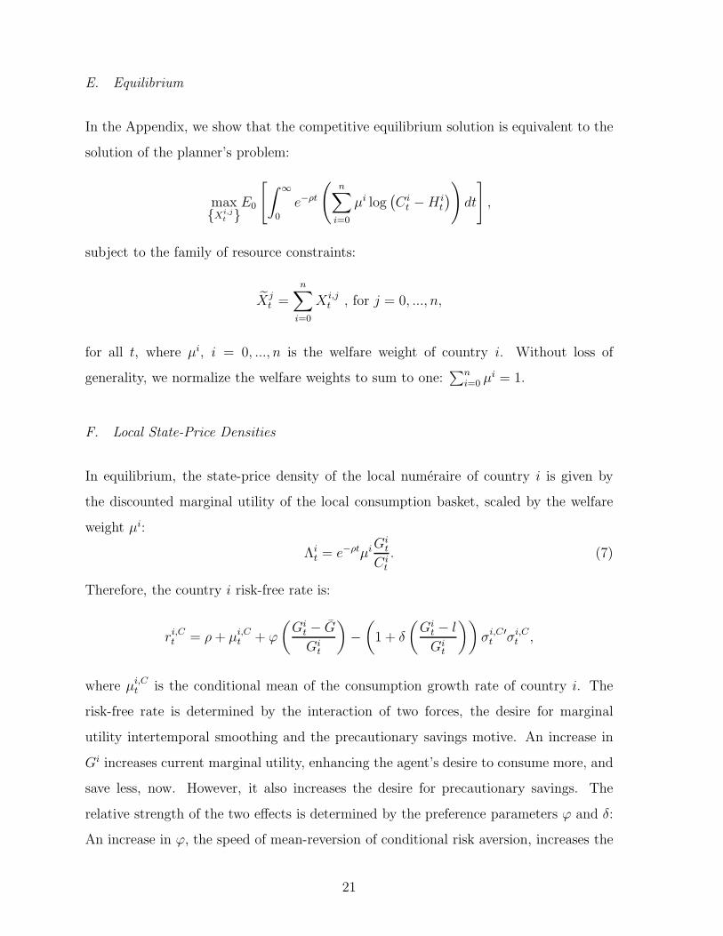
E. Equilibrium

In the Appendix, we show that the competitive equilibrium solution is equivalent to the

solution of the planner’s problem:

maxXi,j

t E0

[∫∞

0

e−ρt

(n∑

i=0

µi log(C i

t −H it

))dt

],

subject to the family of resource constraints:

Xjt =

n∑

i=0

X i,jt , for j = 0, ..., n,

for all t, where µi, i = 0, ..., n is the welfare weight of country i. Without loss of

generality, we normalize the welfare weights to sum to one:∑n

i=0 µi = 1.

F. Local State-Price Densities

In equilibrium, the state-price density of the local numeraire of country i is given by

the discounted marginal utility of the local consumption basket, scaled by the welfare

weight µi:

Λit = e−ρtµiG

it

C it

. (7)

Therefore, the country i risk-free rate is:

ri,Ct = ρ+ µi,Ct + ϕ

(Gi

t − G

Git

)−

(1 + δ

(Gi

t − l

Git

))σi,C′

t σi,Ct ,

where µi,Ct is the conditional mean of the consumption growth rate of country i. The

risk-free rate is determined by the interaction of two forces, the desire for marginal

utility intertemporal smoothing and the precautionary savings motive. An increase in

Gi increases current marginal utility, enhancing the agent’s desire to consume more, and

save less, now. However, it also increases the desire for precautionary savings. The

relative strength of the two effects is determined by the preference parameters ϕ and δ:

An increase in ϕ, the speed of mean-reversion of conditional risk aversion, increases the

21

importance of the smoothing motive, as it raises the probability that future marginal

utility will be lower, while an increase in δ, the sensitivity of risk aversion changes

to consumption shocks, increases the conditional variability of marginal utility and,

therefore, the agent’s incentive to accumulate precuationary savings.

The local market price of risk is given by:

ηit =

(1 + δ

(Gi

t − l

Git

))σi,Ct ,

and has two familiar components. The first component is the conditional sensitivity of

the price of risk to consumption growth variability and is increasing in conditional risk

aversion Gi. In the absence of external habit formation, the sensitivity would be constant

and equal to one, the relative risk aversion implied by log utility. However, external habit

formation induces time variation in conditional risk aversion and, thus, to the sensitivity

of the price of risk. The second component, conditional consumption growth volatility, is

determined by the degree of optimal international risk sharing, which, in turn, depends

on the interaction between preference home bias and external habit formation.

G. Global Risk Factors

Note that it holds that:

Λt = e−ρtµiGit

C it

1

P it

.

Rearranging and summing over all countries, we can show that the global numeraire

state-price density is increasing in global conditional risk aversion and decreasing in

global consumption expenditure:

Λt = e−ρtGWt

CWt

,

where we define global conditional risk aversion GW as the welfare-weighted average of

all countries’ conditional risk aversions,

GWt ≡

n∑

i=0

µiGit

22

while the global consumption expenditure is:

CWt ≡

n∑

i=0

(C i

tPit

)=

n∑

i=0

(Xj

tQjt

)

and, given market clearing, equals the value of the global endowment.

We will focus on the properties of the excess currency return, defined as the return

of the foreign money market account in units of the domestic numeraire in excess of the

domestic risk-free rate:

dRit = η′t

(ηt − ηit

)dt+

(ηt − ηit

)′

dBt.

As discussed above, the currency risk premium is determined by the exposure of the

currency return to the two global risk factors, global risk aversion and global consumption

expenditure:

Et

(dRi

t

)= −Et

(dRi

t

dΛt

Λt

)= λC

t βi,Ct + λG

t βi,Gt .

The price of the exposure to global consumption expenditure innovations is positive, as

bad states of the world are associated with low global consumption expenditure, while

the price of the exposure to global risk aversion innovations is negative, as bad states

entail high global conditional risk aversion:

λCt ≡ vart

(dCW

t

CWt

), λG

t ≡ −vart

(dGW

t

GWt

).

H. Global Risk Aversion and Exchange Rate Second Moments

In this section, we explore the association between global risk aversion and the condi-

tional second moments of exchange rate changes. We consider a global economy of 3

countries, the domestic one and 2 foreign ones. To trace the sensitivity of key moments

on global risk aversion, we assume that all 3 countries have identical conditional risk

aversion: Git = GW

t for all i. Eliminating all cross-sectional heterogeneity in conditional

risk aversion allows us to abstract from cross-country insurance effects and focus ex-

clusively on the forces that shape optimal international risk sharing. Given that all

23

countries have access to complete financial markets, countries are able to achieve the

optimal level of international risk sharing. However, given preference home bias, optimal

risk sharing is not identical to perfect consumption pooling: there is a tension between

the desire to share risk, which would imply perfect consumption pooling under preference

homegeneity, and preference home bias, which induces consumption home bias.

I. The Effect of Global Risk Aversion

First, we consider symmetrically home biased preferences.9 The results are presented

in Figure 4; the horizontal axis represents the value of Git, ranging from 20 to 100.

Panels A, B, C and D present the conditional variance and correlation of consumption

growth rates and SDFs across countries. As global risk aversion increases, the desire

to share risk becomes stronger: as a result, cross-country consumption growth and

SDF correlations increase, sharply initially, more slowly afterwards (Panels B and D,

respectively). Increased global risk aversion generates two opposing effects on conditional

SDF volatility ηi: increased international risk sharing decreases the conditional variance

of consumption growth rates (Panel A), which tends to reduce ηi, but the reduction in

consumption risk is not enough to balance the increase in the sensitivity component of

the SDF, so conditional SDF variance increases (Panel C).

[Insert Figure 4 approximately here.]

Panels E, F, G and H present the second moments of real exchange rates and their

determinants. The amount of non-shared risk between the domestic country and foreign

country i can be decomposed into the amount of aggregate risk and the proportion of

the aggregate risk that is not shared. The amount of aggregate risk of the domestic

country and foreign country i is defined as:

RP i,0t ≡ vart

(dΛi

t

Λit

)+ vart

(dΛ0

t

Λ0t

)= ηi′t η

it + η0′t η

0t .

9We set ai,i = 0.8 for all i and ai,j = 0.1 for all i 6= j. The rest of the parameters are calibrated asin Table 6.

24

The proportion of aggregate risk that is shared is given by the Brandt, Cochrane and

Santa-Clara (2006) international risk sharing index:

RSi,0t = 1−

(σit)

2

vart

(dΛi

t

Λit

)+ vart

(dΛ0

t

Λ0t

) = 1−(ηit − η0t )

′

(ηit − η0t )

ηi′t ηit + ηi′t η

0t

.

The index ranges between 0, in which case there is no risk sharing between the two

countries, and 1, in which case risk sharing between the two countries is perfect. Thus,

conditional exchange rate volatility is the product of the proportion of aggregate risk

not shared times the amount of aggregate risk:

(σit

)2= (1− RSi,0

t )RP i,0t .

As global risk aversion increases, the decrease in consumption risk is not enough

to offset the effect of the increase of global risk aversion, so the pricing component

increases (Panel G). On the other hand, increased international risk sharing decreases

the risk sharing component (Panel H). The risk pricing component is the dominant one,

leading to an increase of the conditional variance of exchange rates (Panel E).

Similarly, conditional exchange rate covariance can be written as:

γi,jt =

1

2(1−RSi,0

t )RP i,0t +

1

2(1−RSj,0

t )RP j,0t −

1

2(1−RSi,j

t )RP i,jt ,

so it depends on all bilateral risk pricing (RP i,0, RP j,0, RP i,j) and risk sharing (RSi,0,

RSj,0, RSi,j) terms. As before, the risk pricing terms dominate, so the conditional

exchange rate covariance γ1,2 is also increasing in global risk aversion (Panel E). Given

identical conditional risk aversion across countries, conditional real exchange correlation

only depends on consumption growth moments and, due to symmetry, it is constant and

equal to 0.5, irrespective of the value of global conditional risk aversion (Panel F).

25

I.1. Asymmetric Home Bias

Assuming identical conditional risk aversion across countries, variation in global risk

aversion induces variation in conditional real exchange rate correlation if preference het-

erogeneity is asymmetric across countries. Two effects worth mentioning are the size

effect and the preference home bias effect. If the domestic country has a higher equi-

librium welfare weight than the foreign countries, but is equally home biased to them,10

then conditional real exchange rate correlation is decreasing in global risk aversion (see

Figure 5, Panel A and B). On the other hand, if all countries have identical welfare

weights, but the domestic country is more home biased than the foreign countries,11

conditional real exchange rate correlation is increasing in global risk aversion (see Fig-

ure 5, Panel C and D).

[Insert Figure 5 approximately here.]

J. Simulation Results

We simulate a global economy of 22 countries, the domestic one and 21 foreign ones,

in the monthly frequency. The log endowment growth processes are specified to be

symmetric and have constant first and second moments:

d log Xjt = µdt+ σjdBt, j = 0, 1, . . . , 21,

where σj is a 22 × 1 vector such that σj [j, 1] = σ and σj [j′, 1] = σρ for all j′ 6= j.

Regarding preferences, we specify the preference matrix A so that the domestic country

10We set A =

0.80 0.10 0.100.15 0.80 0.050.15 0.05 0.80

. As a result, the welfare weights are: µ0 = 0.43 and µ1 = µ2 =

0.29. The rest of the parameters are calibrated as in Table 6.

11We set A =

0.90 0.05 0.050.05 0.80 0.150.05 0.15 0.80

. As a result, the welfare weights are µi = 1/3 for all i. The rest

of the parameters are calibrated as in Table 6.

26

(US) is more home-biased and larger than the foreign countries; all foreign countries are

symmetric. Specifically, we set

A =

0.8700 0.0062 ... 0.0062

0.0506 0.6000 ... 0.0175

... ... ... ...

0.0506 0.0175 0.0175 0.6000

so the domestic and foreign country home bias is 0.87 and 0.6, respectively, and the

domestic country has an equilibrium welfare weight µ0 = 0.28.12 The other calibration

parameters are reported in Table 6. Notably, we set the parameter of conditional risk

aversion mean-reversion, ϕ, equal to 0.03, so conditional risk aversion is very persis-

tent and, thus, the intertemporal smoothing component of the risk-free rate is weak.

On the other hand, we set δ, the sensitivity parameter of conditional risk aversion to

consumption growth shocks to 120, implying a strong precautionary savings motive.

[Insert Table 6 approximately here.]

J.1. Sorting on Conditional Global Risk Aversion Betas

As discussed previously, risk premia compensate investors for exposure to two priced

global risk factors, the global consumption expenditure factor and the global risk aversion

factor. In our calibration, the price of the latter risk factor is an order of magnitude

higher than the price of the former one. This calibration is typical in models that rely on

the variability of the surplus consumption ratio in order to generate substantial volatility

in the SDF, given smooth consumption growth. As a result, the cross-section of currency

returns largely mirrors the cross-section of global risk aversion betas.

12The preference matrix A is calibrated using annual data from 1999 to 2010 on GDP, imports ofgoods and services and exports of goods services. The US preference home bias, 0.87, corresponds tothe time-series average of the US openness ratio 0.5(Imports+Exports)/GDP over the sample. Theforeign preference home bias, 0.6, corresponds to the cross-sectional average of 20 countries’ (all theforeign countries in our empirical analysis, bar Singapore) average openness ratio. Finally, the domesticwelfare weight corresponds to the US share of global GDP over the sample period.

27

Table 7 illustrates that point: we do a monthly sort of the 21 foreign currencies

into 4 portfolios according to their conditional global risk aversion beta, with Portfolio

1 containing the currencies in the lowest βi,G quartile and Portfolio 4 containing the

currencies in the highest βi,G quartile. As expected, there is a monotonic negative

relationship between global risk aversion betas and average currency portfolio returns:

the riskiest portfolio, Portfolio 1, which has the lowest risk aversion beta and, thus, the

highest adverse exposure to the global risk aversion factor outperforms Portfolio 4, which

provides the best hedge against global risk aversion, by about 10% in annual terms.

The calibrated parameters generate conditional real exchange rate correlation that

is increasing in global risk aversion. Figure 5 (Panel E and F) shows the dependence of

conditional real exchange rate moments on global risk aversion, assuming country risk

aversions are identical. The US is calibrated as both a relatively large and home-biased

country, two characteristics that have opposing effects on the dependence of conditional

real exchange rate correlation on global risk aversion, but, in our calibration, the relative

home-bias effect dominates and all real exchange rate second moments are increasing in

global risk aversion.

[Insert Table 7 approximately here.]

J.2. Sorting on Forward Discounts

Finally, we explore the ability of our model to address the forward premium puzzle,

as illustrated in Table 1. Table 8 reports the summary statistics on portfolios sorted

on interest rate differentials (forward discounts): Portfolio 1 contains currencies ranked

in the bottom forward discount quantile (low interest rate currencies), while Portfolio

4 contains the high interest rate currencies. Since the cross-section of currency risk

premiums is largely determined by the cross-section of global risk aversion betas, Table

8 implies that high (low) interest rate currencies have low (high) global risk aversion

betas, i.e. that they depreciate (appreciate) in bad states of the world, when global risk

aversion is high.

[Insert Table 8 approximately here.]

28

To understand the connection between global risk aversion betas and risk-free rates,

we can abstract from the second-order consumption growth terms and write the global

risk aversion beta of currency return i as:

βi,Gt =

covt

(dRi

t,dGW

t

GWt

)

vart

(dGW

t

GWt

) 'covt

(dGi

t

Git

−dGW

t

GWt

,dGW

t

GWt

)

vart

(dGW

t

GWt

) = ρt

(dGi

t

Git

,dGW

t

GWt

) σt

(dGi

t

Git

)

σt

(dGW

t

GWt

) − 1.

If international risk sharing is sufficiently high in equilibrium, Stathopoulos (2011) shows

that the growth rate of conditional risk aversion is very correlated across countries, so

the correlation term above is close to 1 and we can write:

βi,Gt '

σt

(dGi

t

Git

)

σt

(dGW

t

GWt

) − 1.

Since the conditional volatility of the growth rate of conditional risk aversion is increasing

in the level of conditional risk aversion, the expression above suggests that the currencies

of countries with high conditional risk aversion compared to the rest of the world will

tend to have a positive βi,G and, thus, provide a hedge against increases in global risk

aversion, while the currencies of countries with low relative conditional risk aversion will

tend to be very exposed to adverse fluctuations of global risk aversion (negative βi,G)

and, thus, will command high risk premia.

After establishing a positive relationship between the cross-section of global risk aver-

sion betas and the cross-section of conditional risk aversion levels, we need to establish

a negative relationship between the level of conditional risk aversion and the level of the

risk-free rate in each country. As Verdelhan (2010) shows, such a negative relationship

arises if the precautionary savings motive dominates the intertemporal smoothing mo-

tive and, as a result, real interest rates are procyclical. In short, if real interest rates are

procyclical, low interest rate currencies provide a conditional hedge against increases of

global risk aversion, whereas high interest rate currencies are conditionally riskier. As

mentioned in a previous section, the cyclical behavior of the real interest rate depends on

the relative strength of the intertemporal smoothing motive vis-a-vis the precautionary

savings motive and, thus, largely on the values of the preference parameters ϕ and δ.

29

Our calibration parameters imply a dominant precautionary savings motive. As a

result, the high interest rate currency portfolio (Portfolio 4) contains the currencies of

low conditional risk aversion countries and, thus, is very exposed to global risk aversion

risk, while the low interest rate portfolio (Portfolio 1) contains the currencies of high

risk aversion countries and thus, provides a good hedge against increases in global risk

aversion and has a negative average return.

IV. Conclusion

We show that FX correlation risk is priced in the cross section of currency returns.

We construct an FX correlation risk factor from implied correlations of major currency

pairs and show that its price is negative and economically significant (-1% per year).

Sorting currencies into portfolios on the basis of their exposure to this FX correlation

factor, we find that a strategy which is long low FX correlation beta currencies and

short high FX correlation beta currencies yields attractive returns and Sharpe ratios.

Furthermore, we address the forward premium puzzle by showing that high interest rate

currencies are highly exposed to FX correlation risk, whereas low interest rate currencies

provide a hedge against adverse FX correlation innovations.

Motivated by our empirical findings, we propose a general equilibrium model that

links the conditional moments of real exchange rates with global conditional risk aversion.

We show that, in our calibration, hedging against increases in conditional exchange rate

second moments proxies for hedging against increases in global risk aversion. If interest

rates are procyclical, high interest rate currencies command high risk premia due to

their high exposure to the global risk aversion factor, justifying the empirically observed

violations from uncovered interest rate parity.

30

References

Andersen, T., and T. Bollerslev (1998): “Answering the Skeptics: Yes, Standard Volatil-ity Models Do Provide Accurate Forecasts,” International Economic Review, 39, p. 885 –905.

Andersen, T., T. Bollerslev, F. Diebold, and P. Labys (2000): “Exchange RateReturns Standardized by Realized Volatility are (Nearly) Gaussian,” Multinational Finance

Journal, 4, p. 159 – 179.

Ang, A., R. Hodrick, Y. Xing, and X. Zhang (2006): “The Cross-Section of Volatilityand Expected Returns,” Journal of Finance, 61, p. 259 – 299.

Bank for International Settlement (2010): “Report on Global Foreign Exchange Mar-ket Activity in 2010,” Triennial Central Bank Survey.

Bansal, R., and I. Shaliastovich (2011): “A Long-Run Risks Explanation of PredictabilityPuzzles in Bond and Currency Markets,” Working Paper, Duke University.

Brandt, M., J. Cochrane, and P. Santa-Clara (2006): “International Risk SharingIs Better Than You Think, or Exchange Rates are too Smooth,” Journal of Monetary

Economics, 53, p. 671 – 698.

Brandt, M. W., and F. X. Diebold (2006): “A No-Arbitrage Approach to Range-BasedEstimation of Return Covariances and Correlations,” Journal of Business, 79, p. 61 – 73.

Britten-Jones, M., and A. Neuberger (2000): “Option Prices, Implied Price Processes,and Stochastic Volatility,” Journal of Finance, 55, 839–866.

Brunnermeier, M., S. Nagel, and L. H. Pedersen (2009): “Carry Trades and CurrencyCrashes,” NBER Macroeconomics Annual 2008, 23, p. 313 – 347.

Burnside, C. (2011): “Carry Trades and Risk,” NBER Working Paper 17278.

Burnside, C., M. Eichenbaum, I. Kleshchelski, and S. Rebelo (2011): “Do PesoProblems Explain the Returns to the Carry Trade?,” Review of Financial Studies, 24, p.853 – 891.

Cenedese, G., L. Sarno, and I. Tsiakas (2012): “Average Variance, Average Correlationand Currency Returns,” Working Paper, Cass Business School.

Colacito, R., and M. M. Croce (2009): “Six Anomalies looking for a model: A consump-tion based explanation of International Finance Puzzles,” Working Paper, UNC.

(2010): “Risk Sharing for the Long-Run: A General Equilibrium Approach to Inter-national Finance with Recursive Preferences and Long-Run Risks,” Working Paper, UNC.

Corte, P. D., L. Sarno, and I. Tsiakas (2011): “Spot and Forward Volatility in ForeignExchnage,” Journal of Financial Economics, 100, p. 496 – 513.

Danielsson, J., and R. Payne (2001): “Measuring and Explaining Liquidity on an Elec-tronic Limit Order Book: Evidence from Reuters D2000-2,” Working Paper, London Schoolof Economics.

31

Demeterfi, K., E. Derman, M. Kamal, and J. Zhou (1999): “A Guide to Volatility andVariance Swaps,” Journal of Derivatives, 6, p. 9 – 32.

Driessen, J., P. Maenhout, and G. Vilkov (2009): “The Price of Correlation Risk:Evidence from Equity Options,” Journal of Finance, 64, p. 1377 – 1406.

Fama, E., and J. MacBeth (1973): “Risk, Return, and Equilibrium: Empirical Tests,”Journal of Political Economy, 81, p. 607 – 636.

Fama, E. F. (1984): “Forward and Spot Exchange Rates,” Journal of Monetary Economics,14, p. 319 – 338.

Farhi, E., S. Fraiberger, X. Gabaix, R. Ranciere, and A. Verdelhan (2009): “CrashRisk in Currency Markets,” Working Paper, Harvard University.

Farhi, E., and X. Gabaix (2011): “Rare Disasters and Exchange Rates,” Working Paper,Harvard University.

Garman, M. B., and S. W. Kohlhagen (1983): “Foreign Currency Option Values,” Journal

of International Money and Finance, 2, p. 231 – 237.

Goodhart, C., T. Ito, and R. Payne (1995): “One Day in June, 1993: A Study of theWorking of Reuters 2000-2 Electronic Foreign Exchange Trading System,” NBER TechnicalWorking Papers, 179.

Jiang, G., and Y. Tian (2005): “Model-Free Implied Volatility and Its Information Content,”Review of Financial Studies, 18, p. 1305 – 1342.

Jurek, J. (2009): “Crash-Neutral Currency Carry Trades,” Working Paper, Princeton Uni-versity.

Lustig, H., N. Roussanov, and A. Verdelhan (2011): “Common Risk Factors in Cur-rency Markets,” forthcoming, Review of Financial Studies.

(2012): “Countercylical Currency Risk Premia,” Working Paper, UCLA.

Lustig, H., and A. Verdelhan (2007): “The Cross-Section of Foreign Currency Risk Premiaand Consumption Growth Risk,” American Economic Review, 97, p. 89 – 117.

Martin, I. (2011): “The Forward Premium Puzzle in a Two-Country World,” Working Paper,Stanford University.

Menkhoff, L., L. Sarno, M. Schmeling, and A. Schrimpf (2011): “Carry Trades andGlobal Foreign Exchnage Volatility,” forthcoming, Journal of Finance.

Menzly, L., T. Santos, and P. Veronesi (2004): “Understanding Predictability,” Journal

of Political Economy, 112, p. 1 – 47.

Roll, R. (1984): “A Simple Implicit Measure of the Effective Bid-Ask Spread in An EfficientMarket,” Journal of Finance, 39, p. 1127 – 1139.

Stathopoulos, A. (2011): “Asset Prices and Risk Sharing in Open Economies,” WorkingPaper, University of Southern California.

(2012): “Portfolio Home Bias and External Habit Formation,” Working Paper, Uni-versity of Southern California.

32

Verdelhan, A. (2010): “A Habit-Based Explanation of the Exchange Rate Risk Premium,”Journal of Finance, 65, p. 123 – 146.

Verdelhan, A. (2011): “The Share of Systematic Variation in Bilateral Exchange Rates,”Working Paper, MIT.

Wachter, J. A. (2006): “A Consumption-Based Model of the Term Structure of InterestRates,” Journal of Financial Economics, 79, p. 365 – 399.

Yu, J. (2011): “A Sentiment-Based Explanation of the Forward Premium Puzzle,” WorkingPaper, University of Minnesota.

33

Appendix A Proofs

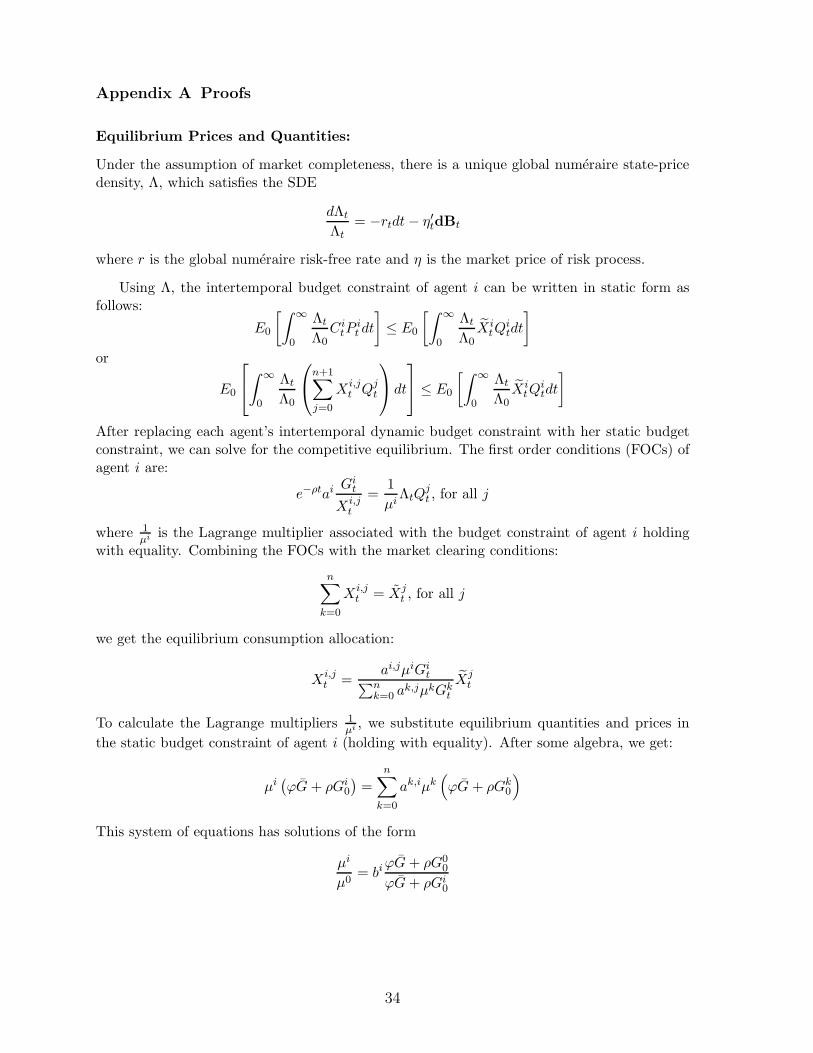
Equilibrium Prices and Quantities:

Under the assumption of market completeness, there is a unique global numeraire state-pricedensity, Λ, which satisfies the SDE

dΛt

Λt

= −rtdt− η′tdBt

where r is the global numeraire risk-free rate and η is the market price of risk process.

Using Λ, the intertemporal budget constraint of agent i can be written in static form asfollows:

E0

[∫∞

0

Λt

Λ0CitP

it dt

]≤ E0

[∫∞

0

Λt

Λ0Xi

tQitdt

]

or

E0

∫

∞

0

Λt

Λ0

n+1∑

j=0

Xi,jt Qj

t

dt

≤ E0

[∫∞

0

Λt

Λ0Xi

tQitdt

]

After replacing each agent’s intertemporal dynamic budget constraint with her static budgetconstraint, we can solve for the competitive equilibrium. The first order conditions (FOCs) ofagent i are:

e−ρtaiGi

t

Xi,jt

=1

µiΛtQ

jt , for all j

where 1µi is the Lagrange multiplier associated with the budget constraint of agent i holding

with equality. Combining the FOCs with the market clearing conditions:

n∑

k=0

Xi,jt = Xj

t , for all j

we get the equilibrium consumption allocation:

Xi,jt =

ai,jµiGit∑n

k=0 ak,jµkGk

t

Xjt

To calculate the Lagrange multipliers 1µi , we substitute equilibrium quantities and prices in

the static budget constraint of agent i (holding with equality). After some algebra, we get:

µi(ϕG+ ρGi

0

)=

n∑

k=0

ak,iµk(ϕG + ρGk

0

)

This system of equations has solutions of the form

µi

µ0= bi

ϕG+ ρG00

ϕG+ ρGi0

34

where the vector b = [b1, b2, ..., bn]′ is the unique solution of

b =

a0,1 a1,1 ... an,1

a0,2 a1,2 ... an,2

... ... ... ...a0,n a1,n ... an,n

[

1b

]

The budget constraint determines only the ratios µi

µ0 . To pin down the values for the Lagrange

multipliers, we impose the normalization∑n

i=0 µi = 1.

It can easily be shown that, if the planner takes the law of motion for each agent’s inversesurplus consumption ratio as exogenous, the planner’s problem solution is equivalent to thecompetitive equilibrium solution if each country’s welfare weight is set equal to µi.

Equilibrium consumption processes:

Since equilibrium consumption C = [C0, ..., Cn]′ is a function of the vector of conditionalrisk aversion G = [G0, ..., Gn]′, we need to solve for the fixed point that satisfies both theequilibrium consumption allocations and the law of motion for G. By the definition of theconsumption baskets, we have:

Ci ≡

n∏

j=0

(Xi,j

)ai,j , for all i

so, applying Ito’s lemma and equating the diffusion terms, we get, after some algebra:

σCt =(Ψ−1

t A)σXt

where σCt is the (n+ 1)×m consumption volatility matrix

σCt =

σ0,C′

t

...

σn,C′

t

σXt is the (n+ 1)×m endowment volatility matrix

σXt =

σ0,X′

t

...

σn,X′

t

and, finally, Ψ is the (n+ 1)× (n + 1) matrix defined as

Ψt = [ψi,j] = ψi−1,j−1t

where

ψi,it ≡ 1 +

1−

n∑

j=0

ai,jai,jµiGit∑n

k=0 ak,jµkGk

t

δ

(Gi

t − l

Git

)

and

ψi,i′

t ≡ −

n∑

j=0

ai,jai′,jµi

′

Gi′

t∑nk=0 a

k,jµkGkt

δ

(Gi′

t − l

Gi′t

), i 6= i′

35

Appendix B Tables

Table 1

Summary Statistics Carry Trade Portfolios

This table reports summary statistics for portfolios sorted on time t − 1 forward dis-counts. We also report annualized Sharpe Ratios (SR) and the first order autocorrelationcoefficient (AC(1)). Portfolio 1 contains 25% of all the currencies with the lowest forwarddiscounts whereas Portfolio 4 contains currencies with the highest forward discounts. Allreturns are excess returns in USD. DOL denotes the average return of the four currencyportfolios, HmL denotes a long-short portfolio that is short in Pf1 and long in Pf4. Datais sampled monthly and runs from January 1999 to December 2010.

Pf1 Pf2 Pf3 Pf4 DOL HmL

Mean -0.004 0.027 0.048 0.088 0.040 0.092StDev 0.068 0.081 0.080 0.097 0.073 0.078Skewness 0.108 -0.208 -0.120 -1.445 -0.435 -1.070Kurtosis 2.613 3.632 4.808 9.394 4.683 6.773SR -0.065 0.334 0.596 0.908 0.540 1.189AC(1) 0.10 0.07 0.18 0.28 0.19 0.29

36

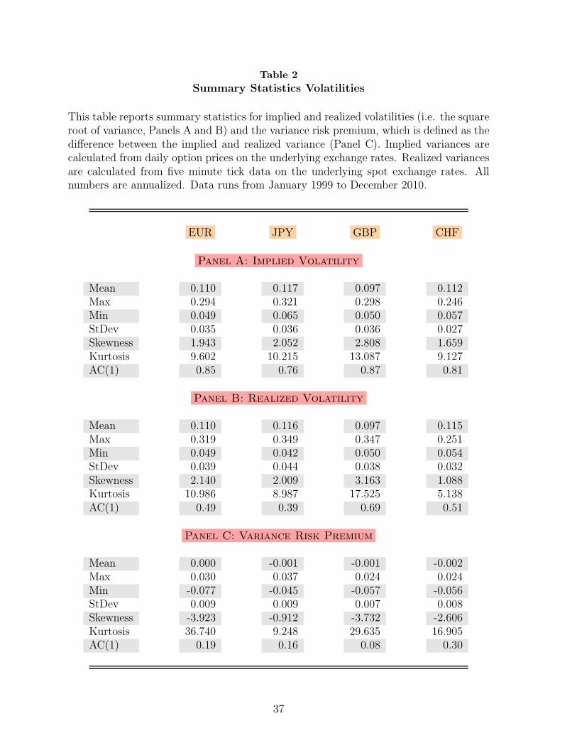
Table 2

Summary Statistics Volatilities

This table reports summary statistics for implied and realized volatilities (i.e. the squareroot of variance, Panels A and B) and the variance risk premium, which is defined as thedifference between the implied and realized variance (Panel C). Implied variances arecalculated from daily option prices on the underlying exchange rates. Realized variancesare calculated from five minute tick data on the underlying spot exchange rates. Allnumbers are annualized. Data runs from January 1999 to December 2010.

EUR JPY GBP CHF

Panel A: Implied Volatility

Mean 0.110 0.117 0.097 0.112Max 0.294 0.321 0.298 0.246Min 0.049 0.065 0.050 0.057StDev 0.035 0.036 0.036 0.027Skewness 1.943 2.052 2.808 1.659Kurtosis 9.602 10.215 13.087 9.127AC(1) 0.85 0.76 0.87 0.81

Panel B: Realized Volatility

Mean 0.110 0.116 0.097 0.115Max 0.319 0.349 0.347 0.251Min 0.049 0.042 0.050 0.054StDev 0.039 0.044 0.038 0.032Skewness 2.140 2.009 3.163 1.088Kurtosis 10.986 8.987 17.525 5.138AC(1) 0.49 0.39 0.69 0.51

Panel C: Variance Risk Premium

Mean 0.000 -0.001 -0.001 -0.002Max 0.030 0.037 0.024 0.024Min -0.077 -0.045 -0.057 -0.056StDev 0.009 0.009 0.007 0.008Skewness -3.923 -0.912 -3.732 -2.606Kurtosis 36.740 9.248 29.635 16.905AC(1) 0.19 0.16 0.08 0.30

37

Table 3

Summary Statistics Correlation

This table reports summary statistics for implied and realized correlations (Panels A and B)and the correlation risk premium, which is the difference between the implied and realizedcorrelation (Panel C). Implied correlations are calculated from daily option prices on the un-derlying exchange rates. Realized correlations are calculated from five minute tick data on theunderlying spot exchange rates. Data is annualized and runs from January 1999 to December2010.

EURJPY EURGBP EURCHF JPYGBP JPYCHF GBPCHF

Panel A: Implied Correlation

Mean 0.396 0.690 0.895 0.303 0.472 0.643Max 0.689 0.863 0.986 0.661 0.811 0.877Min -0.241 0.370 0.541 -0.406 -0.016 0.326StDev 0.191 0.102 0.086 0.216 0.175 0.140Skewness -0.667 -0.632 -2.593 -0.562 -0.683 -0.468Kurtosis 2.957 2.978 10.435 3.218 3.051 2.344AC(1) 0.74 0.78 0.81 0.81 0.70 0.84

Panel B: Realized Correlation

Mean 0.294 0.552 0.728 0.194 0.308 0.473Max 0.640 0.780 0.928 0.580 0.716 0.761Min -0.375 0.165 0.300 -0.355 -0.249 0.110StDev 0.228 0.127 0.126 0.201 0.196 0.135Skewness -0.584 -0.684 -0.680 -0.342 -0.260 -0.113Kurtosis 2.931 2.824 3.013 2.771 2.394 2.296AC(1) 0.82 0.88 0.79 0.82 0.85 0.84

Panel C: Correlation Risk Premium

Mean 0.103 0.139 0.168 0.109 0.164 0.169Max 0.620 0.443 0.537 0.519 0.523 0.491Min -0.221 -0.165 -0.049 -0.345 -0.078 -0.160StDev 0.136 0.117 0.127 0.141 0.125 0.136Skewness 0.681 0.258 0.809 -0.364 0.421 -0.137Kurtosis 4.212 3.079 3.029 4.118 2.829 2.574AC(1) 0.25 0.72 0.77 0.27 0.36 0.68

38

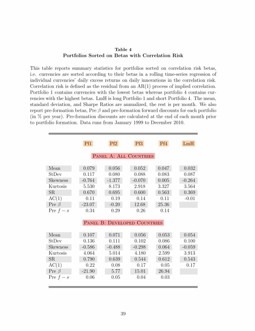
Table 4

Portfolios Sorted on Betas with Correlation Risk

This table reports summary statistics for portfolios sorted on correlation risk betas,i.e. currencies are sorted according to their betas in a rolling time-series regression ofindividual currencies’ daily excess returns on daily innovations in the correlation risk.Correlation risk is defined as the residual from an AR(1) process of implied correlation.Portfolio 1 contains currencies with the lowest betas whereas portfolio 4 contains cur-rencies with the highest betas. LmH is long Portfolio 1 and short Portfolio 4. The mean,standard deviation, and Sharpe Ratios are annualized, the rest is per month. We alsoreport pre-formation betas, Pre β and pre-formation forward discounts for each portfolio(in % per year). Pre-formation discounts are calculated at the end of each month priorto portfolio formation. Data runs from January 1999 to December 2010.

Pf1 Pf2 Pf3 Pf4 LmH

Panel A: All Countries

Mean 0.079 0.056 0.052 0.047 0.032StDev 0.117 0.080 0.088 0.083 0.087Skewness -0.764 -1.377 -0.070 0.005 -0.264Kurtosis 5.530 8.173 2.918 3.327 3.564SR 0.670 0.695 0.600 0.563 0.369AC(1) 0.11 0.19 0.14 0.11 -0.01Pre β -23.07 -0.20 12.68 25.36Pre f − s 0.34 0.29 0.26 0.14

Panel B: Developed Countries

Mean 0.107 0.071 0.056 0.053 0.054StDev 0.136 0.111 0.102 0.086 0.100Skewness -0.586 -0.488 -0.298 0.064 -0.059Kurtosis 4.064 5.014 4.180 2.599 3.913SR 0.790 0.639 0.544 0.612 0.543AC(1) 0.22 0.08 0.17 0.05 0.17Pre β -21.90 5.77 15.01 26.94Pre f − s 0.06 0.05 0.04 0.03

39

Table 5

Estimating the Price of Correlation Risk

Test assets are the four carry trade portfolios based on either all countries or developedcountries only. FIC is the mimicking factor for global correlation innovations, DOL theaverage carry trade portfolio as in Lustig, Roussanov, and Verdelhan (2011). In PanelA, we report factor betas. Panel B reports the Fama and MacBeth (1973) factor priceson the carry return portfolios. Newey-West standard errors are reported in parentheses.Data runs from January 1999 to December 2010.

Panel A: Factor Betas

All Countries Developed Countries

Pf α DOL FIC R2 α DOL FIC R2

1 -0.01 0.94 0.60 0.93 -0.01 0.73 0.02 0.55(0.01) (0.02) (0.02) (0.00) (0.09) (0.01)

2 -0.01 1.08 -0.07 0.88 -0.01 1.00 0.00 0.85(0.01) (0.03) (0.03) (0.00) (0.05) (0.00)

3 0.00 1.03 -0.14 0.86 0.01 1.07 -0.01 0.83(0.00) (0.04) (0.04) (0.00) (0.07) (0.00)

4 0.01 0.94 -0.39 0.97 0.01 1.18 -0.02 0.84(0.01) (0.02) (0.02) (0.00) (0.06) (0.01)

Panel B: Factor Prices

All Countries Developed Countries

DOL FIC R2 DOL FIC R2

0.04 -0.08 0.87 0.01 -0.07 0.95(0.01) (0.01) (0.00) (0.01)

40

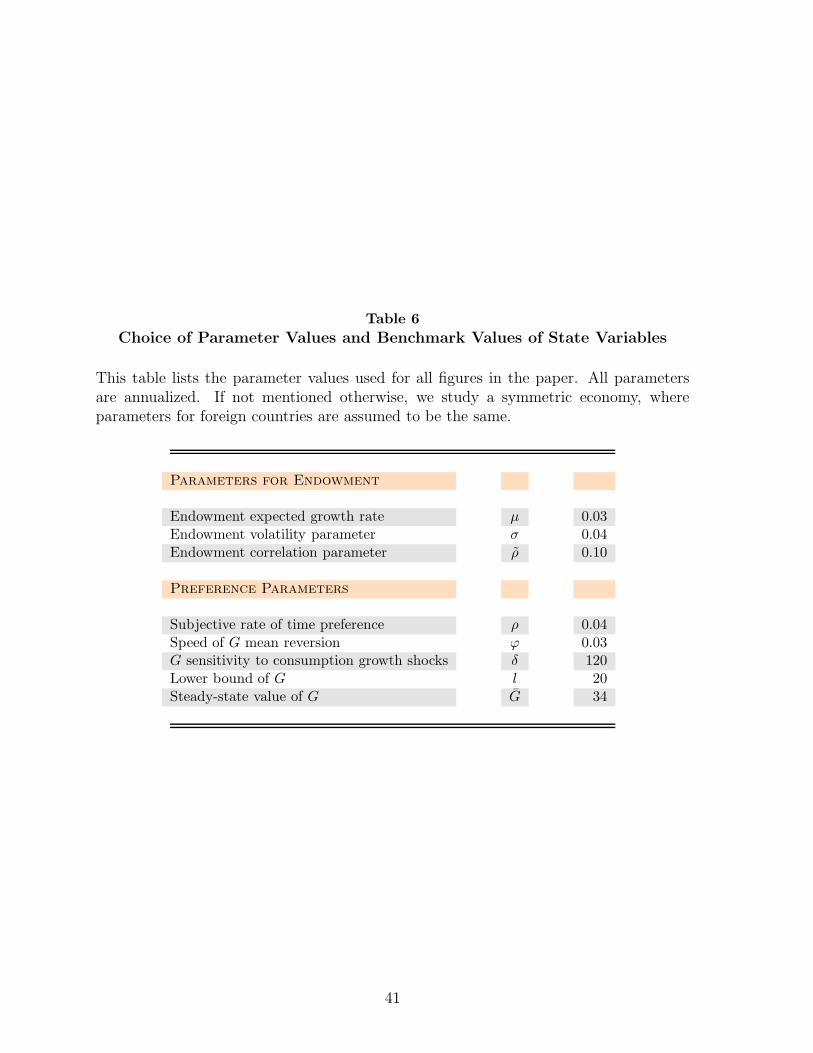
Table 6

Choice of Parameter Values and Benchmark Values of State Variables

This table lists the parameter values used for all figures in the paper. All parametersare annualized. If not mentioned otherwise, we study a symmetric economy, whereparameters for foreign countries are assumed to be the same.

Parameters for Endowment

Endowment expected growth rate µ 0.03Endowment volatility parameter σ 0.04Endowment correlation parameter ρ 0.10

Preference Parameters

Subjective rate of time preference ρ 0.04Speed of G mean reversion ϕ 0.03G sensitivity to consumption growth shocks δ 120Lower bound of G l 20Steady-state value of G G 34

41

Table 7

Summary Statistics Simulated Conditional Risk Aversion Sorted

This table reports summary statistics for portfolios sorted on global risk aversion betasusing 500 simulations of 144 months for 22 countries (21 foreign and one domestic). Wealso report annualized Sharpe Ratios (SR) and the first order autocorrelation coefficient(AC(1)). Portfolio 1 contains 25% of all the currencies with the lowest global risk aversionbeta whereas Portfolio 4 contains currencies with the highest global risk aversion beta.HmL denotes a long-short strategy that is long in Pf1 and short in Pf4.

Pf1 Pf2 Pf3 Pf4 HmL

Mean 0.058 0.009 -0.022 -0.043 0.101StDev 0.036 0.032 0.035 0.036 0.023Skewness -0.657 -0.106 -0.225 -0.162 -0.487Kurtosis 11.383 7.053 10.968 10.801 6.746SR 1.676 0.291 -0.661 -1.255 4.383AC(1) -0.02 -0.01 -0.01 0.01 0.10

42

Table 8

Summary Statistics Simulated Carry Trade Portfolios

This table reports summary statistics for simulated portfolios sorted on time t−1 forwarddiscounts. We also report annualized Sharpe Ratios (SR) and the first order autocorre-lation coefficient (AC(1)). Portfolio 1 contains 25% of all the currencies with the lowestforward discounts whereas Portfolio 4 contains currencies with the highest forward dis-counts. All returns are excess returns in USD. DOL denotes the average return of thefour currency portfolios, HmL denotes a long-short strategy that is long in Pf1 and shortin Pf4.

Pf1 Pf2 Pf3 Pf4 DOL HmL

Mean -0.010 -0.001 0.010 0.024 0.003 0.034StDev 0.061 0.056 0.057 0.061 0.056 0.030Skewness 0.304 0.051 -0.009 -0.051 -0.010 -0.024Kurtosis 4.547 4.780 4.858 4.790 4.618 3.478SR -0.165 -0.164 0.204 0.426 0.083 1.141AC(1) 0.01 0.01 0.01 0.01 -0.01 0.42

43

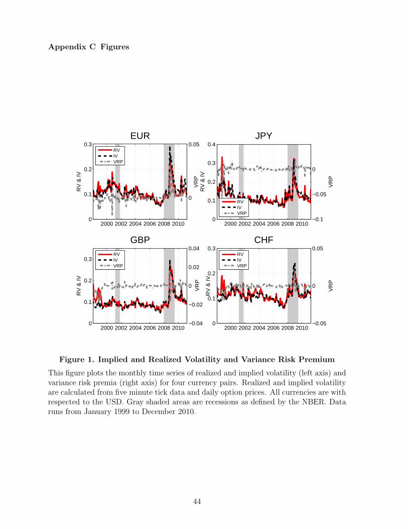
Appendix C Figures

RV

& IV

EUR

2000 2002 2004 2006 2008 20100

0.1

0.2

0.3

VR

P0

0.05RVIVVRP

RV

& IV

JPY

2000 2002 2004 2006 2008 20100

0.1

0.2

0.3

0.4

VR

P

−0.1

−0.05

0

RVIVVRP

RV

& IV

GBP

2000 2002 2004 2006 2008 20100

0.1

0.2

0.3

VR

P

−0.04

−0.02

0

0.02

0.04RVIVVRP

RV

& IV

CHF

2000 2002 2004 2006 2008 20100

0.1

0.2

0.3

VR

P−0.05

0

0.05RVIVVRP

Figure 1. Implied and Realized Volatility and Variance Risk Premium

This figure plots the monthly time series of realized and implied volatility (left axis) andvariance risk premia (right axis) for four currency pairs. Realized and implied volatilityare calculated from five minute tick data and daily option prices. All currencies are withrespected to the USD. Gray shaded areas are recessions as defined by the NBER. Dataruns from January 1999 to December 2010.

44

RC

& IC

EURJPY

2000 2002 2004 2006 2008 2010−1

0

1

CR

P

−0.5

0

0.5

RCICCRP

RC

& IC

EURGBP

2000 2002 2004 2006 2008 20100

0.5

1

CR

P

−0.5

0

0.5

RCICCRP

RC

& IC

EURCHF

2000 2002 2004 2006 2008 2010

0.5

0.75

1

1.25C

RP

0

0.5

RCICCRP

RC

& IC

JPYGBP

2000 2002 2004 2006 2008 2010−0.5

0

0.5

1

CR

P

−0.5

0

0.5

RCICCRP

JPYCHF

RC

& IC

2000 2002 2004 2006 2008 2010−0.5

0

0.5

1

RC

& IC

GBPCHF

2000 2002 2004 2006 2008 20100

0.5

1

CR

P

−0.5

0

0.5

RCICCRP

CR

P

−0.5

0

0.5

1

RCICCRP

Figure 2. Implied and Realized Correlation and Correlation Risk Premium

This figure plots the monthly time series of realized and implied correlation (left axis)and correlation risk premium (right axis) for six currency pairs. Realized and impliedcorrelation are calculated from five minute tick data and daily option prices. All cur-rencies are with respected to the USD. Gray shaded areas are recessions as defined bythe NBER. Data runs from January 1999 to December 2010.

45

Vol

atili

ty R

isk

Global Volatility and Correlation Risk

2000 2002 2004 2006 2008 20100

0.1

0.2

0.3

0.4

Cor

rela

tion

Ris

k0

0.2

0.4

0.6

0.8

VolatilityCorrelation

Figure 3. Global Volatility and Correlation Risk

This figure plots the global volatility and correlation risk factor defined as an equalweighted average of individual implied volatility and correlation measures. Impliedvolatilities and correlations are calculated using daily options on different currency pairs.Gray shaded areas are recessions as defined by the NBER. Data is monthly and runsfrom January 1999 to December 2010.

46

20 30 402

2.5

3

3.5x 10

−6Panel A: Consumption Growth Variance

20 30 400.4

0.6

0.8

1Panel B: Consumption Growth Correlation

20 30 400

2

4

6

8x 10

−3 Panel C: SDF Variance

20 30 400.4

0.6

0.8

1Panel D: SDF Correlation

20 30 400

0.5

1

1.5x 10

−5 Panel E: FX Variance & Covariance

20 30 400

0.5

1Panel F: FX Correlation

20 30 400

0.005

0.01

0.015

0.02Panel G: Risk Pricing

20 30 400

0.2

0.4

0.6

0.8 Panel H: 1 − Risk Sharing

varcov

Figure 4. Conditional Global Risk Aversion on Conditional Moments: Sym-metric Preferences

Plots of conditional second moments of consumption growth (Panels A and B), SDF (Panels Cand D) and the real exchange rate (Panels E and F). Panels G and H plot the risk pricing (RP)and risk sharing (1-RS) components of real exchange rate conditional variance, as defined in themain text. The horizontal axis measures global conditional risk aversion, assuming conditionalrisk aversion is equal in all countries, while the vertical axis measures the moment of interest.The global economy comprises 3 countries, the domestic country and 2 foreign countries. Allcountries have symmetrically home-biased preferences, so each country has a welfare weight of1/3.

47

20 30 400

0.000005

0.00001

0.000015Panel A: FX Variance & Covariance, large domestic country

varcov

20 30 400

0.25

0.5

0.75

1Panel B: FX Correlation, large domestic country

20 30 400

0.00002

0.00004

0.00006Panel C: FX Variance & Covariance, home−biased domestic country

varcov

20 30 400.5

0.75

1Panel D: FX Correlation, home−biased domestic country

20 30 400

0.00001

0.00002

0.00003Panel E: FX Variance & Covariance, calibrated preferences

varcov

20 30 400.5

0.75

1Panel F: FX Correlation, calibrated preferences

Figure 5. Conditional Global Risk Aversion on Conditional Moments

Plots of conditional real exchange rate variance and covariance (Panel A), and correla-tion (Panel B). The horizontal axis measures global conditional risk aversion, assumingconditional risk aversion is equal in all countries, while the vertical axis measures themoment of interest. The global economy comprises 3 countries, the domestic countryand 2 foreign countries. Preferences are such that the domestic country has a welfareweight of about 0.43 and each foreign country a welfare weight of about 0.29. All 3countries are equally home-biased. Panel C and D plot FX variance and covariancewhen preferences are such that the domestic country is more home-biased than the 2foreign countries, but all 3 countries have a welfare weight of 1/3. Panel E and F are atthe calibrated moments described in the main text. The global economy comprises 22countries, the domestic country and 21 foreign countries.

48

Online Appendix to “International

Correlation Risk”

High Frequency Data

The exchange rate series consist of the last available mid-quote in each five-minute interval,resulting in 288 observations a day, as trading on the FX markets takes places 24h a day due tothe fact that market opening hours rotate around the globe, from Asia to Europe to Americato Asia and so on. Our choice of these specific series has the following reasons:

1. Equally spaced intervals of five minutes: constructing an artificial time series of equallyspaced observations, called ”sampling in calender time”, is the only time scale lendingitself to multivariate applications. Choosing five-minute intervals is standard in empiricalstudies (see Andersen and Bollerslev, 1998). Although the theory of quadratic variationasks for the highest possible sampling frequency to yield the most accurate volatilitymeasurement, returns measured at intervals shorter than five minutes heavily sufferfrom spurious serial correlation due to market-microstructure effects. These effects, aswell as the optimal sampling frequency will be addressed below.

2. Last quote in every interval: in constructing the equally spaced time series, this so-called”previous-tick interpolation” only uses data available at this very point in time and hencerespects causality. The increase in the number of quotes collected in the O&A databasediminishes the average time interval between two consecutive quotes from 10-20 secondsin 1997 to less than a second in 2010. This gives a hint at how liquid the FX market isand how close to the five-minute time-stamps the last quotes in every interval are. Hence,problems arising from non-synchronous quotations or stale quotes are insignificant.

3. Mid-quotes (instead of transaction prices): as currency trading is mainly OTC, it is hardto get records of true transaction prices. However, Goodhart, Ito, and Payne (1995) andDanielsson and Payne (2001) verify by means of a short data sample from the Reuters2000-2 electronic FX trading platform that the characteristics of the merely indicativequotes of the O&A data closely match the ones of the true transaction prices. In addition,using mid-quotes avoids contamination of the data series with market-microstructurenoise arising from transactions being executed at either the quoted bid or ask price(bid-ask bounces), see e.g. Roll (1984).

To determine periods of inactive trading and hence possible problems with missing data,we find that a quote is recorded for each of the 7 × 24 × 12 = 2016 five-minute intervals of aweek. In the calculation of volatilities and correlations, the days are set to end at 16:00 GMTto match the time of the daily option quotes (all times in this study refer to Greenwich MeanTime). Monday to Friday is treated as business days, while the reduced market activity onSaturdays and Sundays calls for a special treatment of the weekend period, which is defined asusual to last from Friday 21:00 to Sunday 21:00, see Andersen and Bollerslev (1998). Hence,“Mondays” consist of the remaining five hours on Friday from 16:00 to 21:00 and the 19 hoursfrom Sunday 21:00 to Monday 16:00. In the 3% of cases that a quote is not available on abusiness day, the missing value is filled with the previous quote, which induces a slight biastowards zero in the realized (co-)volatility measures.

Implied Volatility Comparison

Subset of Currencies Chosen

To calculate our implied volatility and correlation measures, we rely on the four exchange ratesbetween the EUR, JPY, GBP and CHF vis-a-vis the USD. Even though these five currenciesmake 65% of the total global turnover in the currency market (see BIS, 2010), the questionremains how much these currencies truly capture a global risk. In the following we compare ourseries with the global implied volatility series introduced by JP Morgan. Their global volatilityindex consists of 22 different currencies: Australian Dollar, Brazilian Real, Canadian Dollar,Swiss Franc, Chinese Yuan, Euro, British Pound, Hungarian Forint, Indian Rupee, JapaneseYen, South Korean Won, Mexican Peso, Norwegian Krona, New Zealand Dollar, PhilippinePeso, Polish Zloty, Russian Rouble, Swedish Krona, Singapore Dollar, Turkish Lira, TaiwanDollar and the South African Rand. We plot our global implied volatility index (GlobalIV) together with the JP Morgan IV index (JPMVXYGL) in Figure 1 and report summarystatistics in Table 1.

Impl

ied

Vol

atili

ty

2000 2002 2004 2006 2008 20100

0.1

0.2

0.3

Comparison Implied Volatility Measures

Global IVJPMVXYGL

Figure 1: Global Implied Volatility

JPM OurMean 10.91 11.04StDev 2.73 3.01Max 24.70 28.88Min 6.10 5.72Skewness 1.90 2.33Kurtosis 9.40 12.53

Table 1: Summary Statistics

As one can see immediately, the co-movement of the two time series is very high: The uncondi-tional correlation between the levels is 98% and between the changes it is 90%. This indicatesthat our measure of global implied volatility based on five currencies captures well global risk.

Weighting Scheme to Construct Global Measures

We use an equal weighted average to calculate our global volatility and correlation measures.To check the robustness of this assumption, we apply a turnover weighted average and con-struct the global volatility proxy using equal and turnover weights as the JP Morgan currencyvolatility index. The turnover weights are based on the Bank of International Settlement (BIS)Triennial Central Bank Survey of foreign exchange downloadable on the BIS webpage. Sinceturnover data is only published on a 3 year frequency, we keep the weights constant for 3 yearsand then update the following year when the new data is published. Turnover weights arechosen over trade weights, as they capture demand for the currencies as a function of bothcommercial and financial demand. Figure 2 plots the two time series and Table 2 reports thesummary statistics.

1

Impl

ied

Vol

atili

ty

Different Weighting Scheme

2000 2002 2004 2006 2008 20100

0.1

0.2

0.3

Equal WeightTurnover Weight

Figure 2: Weighting Schemes

Equal Turnover

Mean 11.04 11.05StDev 3.01 3.28Max 28.88 29.78Min 5.72 5.61Skewness 2.33 2.26Kurtosis 12.53 11.74

Table 2: Summary Statistics

The two time series are extremely highly correlated with an unconditional correlation of 99.8%(levels) and 99.7% (changes). The summary statistics are also almost identical. We thereforeconclude that the assumption of an equal weighted average is not driving our results. We alsonote that we cannot perform the same kind of robustness check for the correlation, as the BISonly provides data on currencies either vis-a-vis the U.S. Dollar or the Euro.

Realized Correlation Sorting

In this section, we check whether our sorting procedure is also robust to realized measures ofcorrelation. We apply the same procedure as in Section II.A. of the main paper. Realizedglobal correlation risk is defined as the realized counterpart to equation (6).

The results are reported in Table 3. We note that the results remain qualitatively un-changed. Low exposure currencies yield higher returns than high exposure currencies. TheHmL portfolios are slightly higher for the realized correlation portfolios and the Sharpe ratiosare also slightly higher with an annualized Sharpe ratio of 0.65 for the realized correlationsorted currencies.

Volatility Sorting

We check whether our sorting procedure is robust to volatility sorting, we sort currenciesaccording to their implied and realized volatility exposure. Summary statistics are reportedin Tables 4 and 5. The results are in line with the correlation sorted portfolios: Sharpe ratiosare quite attractive, ranging between 0.5 for the implied volatility sorted LmH portfolio andalmost 0.7 for the realized volatility sorted LmH portfolio. Low exposure currencies have higherexpected returns than high exposure currencies.

Real Carry Returns

We proxy the real forward discount as the nominal forward discount minus the inflationdifferential. We retrieve monthly inflation rates from the International Labour Office (see

2

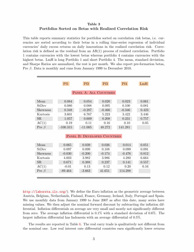
Table 3

Portfolios Sorted on Betas with Realized Correlation Risk

This table reports summary statistics for portfolios sorted on correlation risk betas, i.e. cur-rencies are sorted according to their betas in a rolling time-series regression of individualcurrencies’ daily excess returns on daily innovations in the realized correlation risk. Corre-lation risk is defined as the residual from an AR(1) process of realized correlation. Portfolio1 contains currencies with the lowest betas whereas portfolio 4 contains currencies with thehighest betas. LmH is long Portfolio 1 and short Portfolio 4. The mean, standard deviation,and Sharpe Ratios are annualized, the rest is per month. We also report pre-formation betas,Pre β. Data is monthly and runs from January 1999 to December 2010.

Pf1 Pf2 Pf3 Pf4 LmH

Panel A: All Countries

Mean 0.084 0.054 0.020 0.023 0.061StDev 0.080 0.088 0.095 0.100 0.081Skewness 0.348 -0.287 -0.466 -0.346 0.423Kurtosis 3.601 6.767 5.223 3.422 3.446SR 1.057 0.609 0.208 0.231 0.757AC(1) 0.19 0.11 0.16 0.10 0.05Pre β -100.315 -11.005 48.272 141.281

Panel B: Developed Countries

Mean 0.065 0.039 0.026 0.014 0.051StDev 0.097 0.099 0.108 0.099 0.091Skewness -0.030 -0.200 -0.174 -0.476 0.812Kurtosis 4.003 3.982 3.986 4.280 6.664SR 0.671 0.388 0.237 0.141 0.557AC(1) -0.01 0.13 0.12 0.20 0.16Pre β -89.464 -3.663 41.651 114.288

http://laborsta.ilo.org/). We define the Euro inflation as the geometric average betweenAustria, Belgium, Netherlands, Finland, France, Germany, Ireland, Italy, Portugal and Spain.We use monthly data from January 1999 to June 2007 as after this date, many series havemissing values. We then adjust the nominal forward discount by subtracting the inflation dif-ferential. Inflation differentials on average are very small and mostly not significantly differentfrom zero: The average inflation differential is 0.1% with a standard deviation of 0.6%. Thelargest inflation differential has Indonesia with an average differential of 0.5%.

The results are reported in Table 6. The real carry trade is qualitatively not different fromthe nominal one. Low real interest rate differential countries earn significantly lower returns

3

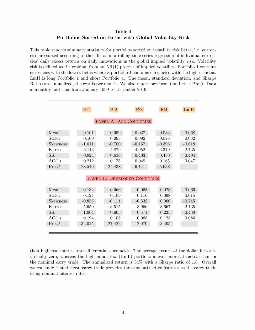
Table 4

Portfolios Sorted on Betas with Global Volatility Risk

This table reports summary statistics for portfolios sorted on volatility risk betas, i.e. curren-cies are sorted according to their betas in a rolling time-series regression of individual curren-cies’ daily excess returns on daily innovations in the global implied volatility risk. Volatilityrisk is defined as the residual from an AR(1) process of implied volatility. Portfolio 1 containscurrencies with the lowest betas whereas portfolio 4 contains currencies with the highest betas.LmH is long Portfolio 1 and short Portfolio 4. The mean, standard deviation, and SharpeRatios are annualized, the rest is per month. We also report pre-formation betas, Pre β. Datais monthly and runs from January 1999 to December 2010.

Pf1 Pf2 Pf3 Pf4 LmH

Panel A: All Countries

Mean 0.101 0.059 0.037 0.033 0.068StDev 0.109 0.093 0.092 0.076 0.032Skewness -1.011 -0.700 -0.167 -0.393 -0.618Kurtosis 6.113 4.879 4.952 3.379 2.735SR 0.924 0.638 0.403 0.430 0.494AC(1) 0.212 0.175 0.049 0.165 0.047Pre β -28.540 -24.438 -6.141 5.638

Panel B: Developed Countries

Mean 0.132 0.066 0.063 0.023 0.066StDev 0.124 0.109 0.110 0.098 0.015Skewness -0.856 -0.111 -0.332 0.006 -0.745Kurtosis 5.650 3.515 3.966 3.667 2.135SR 1.064 0.605 0.571 0.235 0.460AC(1) 0.194 0.108 0.068 0.123 0.086Pre β -32.015 -27.422 -12.070 3.405

than high real interest rate differential currencies. The average return of the dollar factor isvirtually zero, whereas the high minus low (HmL) portfolio is even more attractive than inthe nominal carry trade: The annualized return is 34% with a Sharpe ratio of 1.8. Overallwe conclude that the real carry trade provides the same attractive features as the carry tradeusing nominal interest rates.

4

Table 5

Portfolios Sorted on Betas with Realized Volatility Risk

This table reports summary statistics for portfolios sorted on realized volatility risk betas,i.e. currencies are sorted according to their betas in a rolling time-series regression of individ-ual currencies’ daily excess returns on daily innovations in the global realized volatility risk.Volatility risk is defined as the residual from an AR(1) process of realized volatility. Portfolio1 contains currencies with the lowest betas whereas portfolio 4 contains currencies with thehighest betas. LmH is long Portfolio 1 and short Portfolio 4. The mean, standard deviation,and Sharpe Ratios are annualized, the rest is per month. We also report pre-formation betas,Pre β. Data is monthly and runs from January 1999 to December 2010.

Pf1 Pf2 Pf3 Pf4 LmH

Panel A: All Countries

Mean 0.085 0.048 0.054 0.045 0.040StDev 0.098 0.102 0.089 0.082 0.076Skewness -0.098 -0.889 -0.484 -0.184 0.280Kurtosis 4.635 6.065 5.267 3.775 3.345SR 0.864 0.477 0.609 0.547 0.525AC(1) 0.140 0.222 0.051 0.146 0.131Pre β -41.908 -26.673 -13.646 9.453

Panel B: Developed Countries

Mean 0.123 0.092 0.023 0.055 0.068StDev 0.101 0.131 0.108 0.115 0.099Skewness 0.235 -0.498 -0.867 -0.133 0.133Kurtosis 2.983 6.709 4.931 3.961 3.533SR 1.222 0.697 0.214 0.478 0.688AC(1) 0.146 0.312 0.167 0.035 0.173Pre β -41.606 -28.761 -18.907 6.225

5

Table 6

Summary Statistics Real Carry Trade Portfolios

This table reports summary statistics for portfolios sorted on time t−1 real forward discounts.We also report annualized Sharpe Ratios (SR) and the first order autocorrelation coefficient(AC(1)). Portfolio 1 contains 25% of all the currencies with the lowest forward discountswhereas Portfolio 4 contains currencies with the highest forward discounts. All returns areexcess returns in USD. DOL denotes the average return of the four currency portfolios, HmLdenotes a long-short that is long in Pf1 and short in Pf4. Data runs from January 1999 toDecember 2006.

Pf1 Pf2 Pf3 Pf4 DOL HmL

Mean -0.178 0.007 0.025 0.164 0.005 0.342StDev 0.168 0.074 0.064 0.080 0.074 0.162Skewnewss -2.098 -0.079 -0.089 0.370 -0.433 1.847Kurtosis 6.716 3.370 2.455 3.124 2.859 5.942SR -1.060 0.100 0.390 2.042 0.062 2.105AC(1) 0.80 0.16 0.13 0.29 0.45 0.77

6