international transmission of monetary policy shocks the case of romanian economy

International Transmission of Monetary Policy Shocks

The Case of Romanian Economy

MSc Student: ELENA BOJEŞTEANU

Supervisor: Professor MOISĂ ALTĂR

The Academy of Economic Studies, Bucharest

DOCTORAL SCHOOL OF FINANCE AND BANKING

Bucharest, 2006

Motivation The analysis of comovements using PCA

Identifying monetary policy shocks using a reaction function for the ECB

The transmission of shocks – a SVAR approach

Concluding remarks and further research

Contents

Two-country models:

- Mundell Fleming (1962);- Svensson and van Wijnbergen (1989);- Obstfeld and Rogoff (1995);- Chari, Kehoe and McGrattan (1997, 2000);- Engel and Devereux (2003).

Empirical Investigations:- Cushman and Zha (1997); - Christiano, Eichenbaum and Evans (1996,

1998);- Betts and Devereux (1999);- Bordo and Murshid (2002);- Pesaran et al. (2005).

Key References

The last five years: improved performance in terms of economic expansion, strengthening disinflation, reduction in budget deficit and unemployment.

A small open economy: a degree of financial and commercial openness exceeding 70% in the last 8 years. Main trading partner: European Union (over 70% of the total for exports, and more than 60% of the total imports. Trading currency: more than 60% settlement of exports and imports in euro, and approx. 30%in US dollar.

Capital account liberalization schedule. Romania is increasingly integrating into world markets and more precisely, into European structures.

Question: how do the commercial and financial linkages affect the Romanian main economic indicators? Is there a comovement in the economic variables, a synchronization of business cycles, or Romanian is still in an incipient phase of integration?

Romanian Economy

The method generates a new set of variables, called principal components

PC are orthogonal to each other

Each principal component (pc) is a linear combination of the original variables

The coefficients of each of the linear combinations are called loadings (or weights)

The first principal component explains the greatest amount of the total original variance

The sum of the pc variances equals the total variance of the initial system

Tracing comovements using Principal Component Analysis

The first component loading for Romania is small, which shows a lower correlation with the rest of the system. Sayek and Selover (2002) state that the first principal component might be thought of as the business cycle followed by the Western nations.

For the second component, Romania has a much higher loading than the rest of the countries. The low and positive Romania’s loading on the first component may be a sign that the macroeconomic evolution in this country was in general out of step with the rest of the group.

Tracing comovements using Principal Component AnalysisGDP growth rates

The Principal Components for GDP growth rates in Germany, France, Italy, Hungary, The Netherlands, Austria, UK and Romania

sample 1998:1-2005:4

1 2 3 4 5 6 70

0.1

0.2

0.3

0.4

0.5

0.6

0.7

0.8

0.9

1

Principal Component

Var

ianc

e E

xpla

ined

(%

)

0%

10%

20%

30%

40%

50%

60%

70%

80%

90%

100%

Factor weights

Ge -0.36 -0.19 0.53 Fr -0.42 0.01 -0.22 It -0.41 0.16 0.15 Hu -0.38 0.34 -0.06 Nt -0.38 -0.29 -0.11 At -0.34 0.14 -0.65 UK -0.35 -0.10 0.40

RO 0.04 0.85 0.23

Comp. Percent

explained

Percent explained

(cumm.)

1 46.95 46.95

2 14.83 61.78 3 10.47 72.25

A higher degree of comovement in the financial sector that in the real one. The first principal component explains a substantial portion of the behaviour of interest rates across countries and can be interpreted as the common element of real interest rates.

An atypical pattern for Romania is not out of the question, considering the high correlation with the second component.

The Principal Components for real interest rates in Germany, France, Italy, Hungary, The Netherlands, Austria, UK and Romania

sample 1998:1-2005:4

1 2 3 40

0.1

0.2

0.3

0.4

0.5

0.6

0.7

0.8

0.9

1

Principal Component

Var

ianc

e E

xpla

ined

(%

)

0%

10%

20%

30%

40%

50%

60%

70%

80%

90%

100%

Factor weights

Ge -0.39 0.04 0.17 Fr -0.40 0.11 0.27 It -0.40 0.09 0.10 Hu -0.33 -0.36 0.33 Nt -0.35 0.22 -0.51 At -0.34 0.17 -0.59 UK -0.35 0.22 0.34

RO -0.22 -0.85 -0.24

Comp. Percent

explained

Percent explained

(cumm.)

1 72.55 72.55

2 10.61 83.16 3 7.53 90.69

Tracing comovements using Principal Component AnalysisReal interest rates

Three general strategies for isolating monetary policy shocks:

The recursiveness assumption – based on the estimation of a reaction function for the monetary authorities

- Christiano (1996);- Christiano, Eichenbaum and Evans (CEE,

1996, 1997);- Clarida, Gali and Gertler (1997);- Cushman and Zha (1997).

The narative approach- Romer and Romer (1989)

Long-run neutrality of money- Pagan and Robertson (1995)

Possible Interpretations for Monetary Policy Shocks

An exogenous monetary policy shock, εt - formalized by CEE (1998) as being the disturbance term in an equation of the form:

St = f(—t) + εt ,

where St is the instrument used by the monetary authority and f(—t) is a linear function that captures the policy makers’ responses to variations in different economic variables, as they are known at time t.

An augmented reaction function for the Euro area:

it = (1-ρ)·α+(1-ρ)·β·E[πt+n] + (1-ρ) ·γ·yt + ρ· it + εt .

Identifying the monetary policy shocks using a reaction function for the ECB

Data: ex-post available data survey data

Methodology: GMM for ex-post available data (a popular

technique in the rational-expectation context (Clarida, 1998)). Problem: selection of instruments.

OLS for survey data. Problem: constructing the data.


Studies estimating the reaction function using data before EMU:

Gerdesmeier and Roffia (2003);Gerlach(2003);Surico (2003);

Carstensen and Colavecchio (2005).

Ex-post available data1996:01-2005:04 from ECB and Eurostat databases

Interest rates: the interbank ON interest rate, the 3M EURIBOR, and the 10Y government bond yield

Price indices: annualized HICP and alternatively the core inflation (HICP - All items, excluding energy, food, alcohol and tobacco)

Output gap: from three measures for potential GDP: a Hodrick-Prescott filter (the smoothing parameter equal to 1600 for quarterly data), a linear and a quadratic trend. The three methods yield fairly similar results.

Monetary aggregates: M3; a money gap was also used (the deviation of money growth from the reference value of a constant growth of 4.5% per annum)

Exchange rates: nominal and real effective exchange rate.


Ex-post available data


GMM. The instrument set includes lagged values (up to 4 lags) of the interest rate, inflation and output gap. The results are not very sensitive in respect to the number of lags used as instruments, the J-statistic supports the over-identifying restrictions implied by the model.

The standard errors were computed using the delta method. The J-statistic reported in the table is the minimized value of the objective function, p(J), the null hypothesis that the overidentifying restrictions are satisfied (Hansen’s J-test).

Estimates of forward-looking Taylor rules in the euro area

tttntt iyi )1()1()1(

Specification

2R adj 2R J-stat. p(J)

[2]

4t SE (t-statistic)

0.05 0.00 (10.9)

-1.34 0.24 (-5.57)

0.88 0.11 (7.87)

0.712 0.05 (12.38)

0.83 0.81 (0.143)

0.71

[3]

6t SE (t-statistic)

0.07 0.01 (6.94)

-2.27 0.26 (-4.40)

0.72 0.14 (5.07)

0.81 0.05 (15.69)

0.90 0.89 (0.168)

0.82

[4]

4t , og_qua SE (t-statistic)

0.05 0.00 (14.5)

-1.63 0.20 (-8.06)

0.51 0.06 (7.75)

0.554 0.08 (6.22)

0.67 0.64 (0.164)

0.82

[5]

4t , 1tog SE (t-statistic)

0.06 0.00 (19.8)

-1.70 0.18 (-9.16)

1.28 0.13 (9.18)

0.594 0.113 (5.23)

0.85 0.83 (0.101)

0.82

Ex-post available data


Additional explanatory variables and alternative specifications for Taylor rules in the euro area

ttttntt ixyi )1()1()1()1(

Specification

2R adj2R

J-stat. p(J)

[4] 4t

))(log(neerdxt

SE (t-statistic)

0.05 0.00 (12.9)

-1.29 0.20 (-6.37)

1.06 0.08 (11.9)

0.712 0.05 (12.3)

-0.01 0.05 (-0.21)

0.87 0.85 (0.145)

0.71

[5] 4t

))(log(reerdxt

SE (t-statistic)

0.04 0.01 (9.15)

-1.02 0.26 (-3.82)

0.94 0.09 (9.69)

0.68 0.11 (5.75)

-0.02 0.05 (0.35)

0.88 0.86 (0.126)

0.77

[6] 4t

))3(log(mdxt

SE (t-statistic)

0.05 0.00 (11.3)

-1.37 0.25 (-5.46)

0.86 0.10 (7.75)

0.554 0.08 (6.22)

-0.01 0.07 (-0.13)

0.82 0.80 (0.140)

0.73

[7] 4t

gapmxt _

SE (t-statistic)

0.25 0.04 (5.50)

-0.85 0.18 (4.73)

0.86 0.03 (25.5)

0.594 0.113 (5.23)

-0.007 0.00 (-1.30)

0.82 0.80 (0.140)

0.72

[8] 4t

Meuriborirt 3

SE (t-statistic)

0.05 0.00 (21.5)

-1.58 0.10 (-15.4)

0.95 0.06 (14.2)

0.66 0.04 (16.0)

-

0.76 0.73 (0.24)

0.88

[9] 4t

bondyirt _10

SE (t-statistic)

-0.38 1.78 (-0.2)

20.58 85.28 (0.24)

-13.7 58.39 (-0.2)

0.97 0.08 (11.0)

-

0.75 0.73 (0.165)

0.62

Survey dataSample period 1999:1-2005:4

Quarterly forecasts based only on real-time available information

Solid arguments in favor of using survey data:

- they are more suitable to capture the forward-attitude of the policy makers;

- variables (in particular the series for output) are only available with lags;

- data are often subject to revisions and it may take some quarters before the final series are available.

Inflation: based on the data from the Survey of Professional Forecasters (SPF), measured by the latest available forecast for the current year

A measure of the state of real economy: the Economic Sentiment Indicator (ESI). This economic index appears to be more closely tied to the Governing Council’s interest rate decisions than other variables capturing real economic activity.


Survey data

ESI as a leading indicator for economic activity


The rescaled ESI gap vs. the recursive output gap

-2

-1

0

1

2

1999 2000 2001 2002 2003 2004 2005 2006

Output gap HP recursive ESI gap recursive

Studies estimating the reaction function using survey data:

Carstensen and Colavecchio (2005);Gerdesmeier and Roffia (2005);

Gerlach (2004);Sauer and Sturm (2003).

Survey dataSample period 1999:1-2005:4


Estimated forward-looking Taylor rules using survey data

tttfort iyi )1()1()1(

Explanatory variables

2R Adj2R

[6] c HICP_for ESI_gap

p-value

0.007 (0.31)

1.16 (0.00)

0.50 (0.00)

-

0.33 0.28

[7] - HICP_for ESI_gap

p-value

-

1.56 (0.00)

0.56 (0.00)

-

0.30 0.28

[8] c HICP_for ESI_gap

Ir(-1)

p-value

-0.023 (0.89)

2.68 (0.00)

2.64 (0.00)

0.88 (0.00)

0.97 0.96

[9] - HICP_for ESI_gap

Ir(-1)

p-value

-

1.51 (0.00)

2.19 (0.00)

0.86 (0.00)

0.96 0.96

The first two specifications show the results without partial adjustment. Although this restriction is rejected by the data, the estimates correspond to the original Taylor coefficients. The constant term is found to be statistically insignificant, similar to the findings of Carstensen and Colavecchio (2005).

The equation that best fits the data is considered to be [9], with an interest rate smoothing and no constant term.

Survey data

Identified monetary shocks


Actual vs. Fitted interest rate & the Monetary Shocks

-.008

-.004

.000

.004

.01

.02

.03

.04

.05

1999 2000 2001 2002 2003 2004 2005

Monetary shocks (left axis)Actual int. rate (right axis)Fitted int. rate (right axis)

Survey data


The results show a greater weight attached to the output gap relative to inflation, a conclusion similar to that of the studies using ex-post data.

For some specifications, the constant term is found to be statistically insignificant. The real time forward-looking specifications of the Taylor rule using the SPF

forecasts denote a stabilizing behavior and provide a better description of the actual behavior of the central bank.

Review of Taylor rule estimations for the euro area

- using survey data -

Study Sample period

Carstensen and Colavecchio (2005) Gerdesmeier and Roffia (2005) - 24t

Gerdesmeier and Roffia (2005) - 12t

Sauer and Sturm (2003)

1999:1-2003:2 0.012 1.61 1.34 0.94 (0.019) (0.01) (0.01) (0.00) 1999:1-2003:6 -0.84 2.91 2.02 0.67 (0.97) (0.00) (0.00) (0.00) 1999:1-2003:6 1.87 1.31 1.95 0.71 (0.00) (0.00) (0.00) (0.00) 1999:1-2003:3 0.25 2.31 2.35 0.92 (0.41) (0.00) (0.01) (0.00)

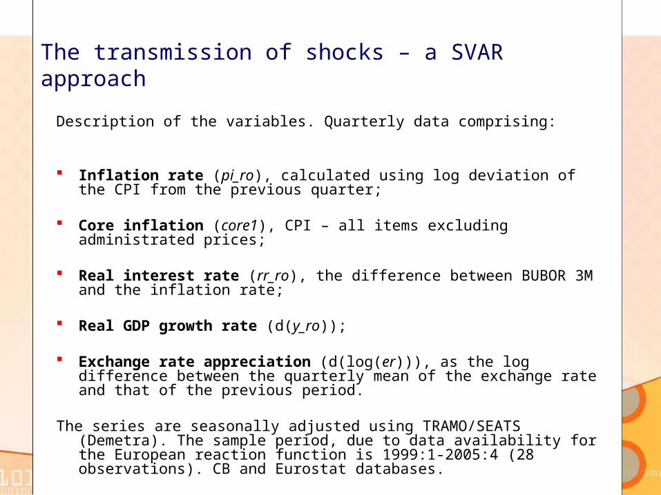
Description of the variables. Quarterly data comprising:

Inflation rate (pi_ro), calculated using log deviation of the CPI from the previous quarter;

Core inflation (core1), CPI – all items excluding administrated prices;

Real interest rate (rr_ro), the difference between BUBOR 3M and the inflation rate;

Real GDP growth rate (d(y_ro));

Exchange rate appreciation (d(log(er))), as the log difference between the quarterly mean of the exchange rate and that of the previous period.

The series are seasonally adjusted using TRAMO/SEATS (Demetra). The sample period, due to data availability for the European reaction function is 1999:1-2005:4 (28 observations). CB and Eurostat databases.


Main three methods to identify the pure innovations:

The recursive approach (the triangular Choleski decomposition)

The structural approach as advocated by Sims and Bernanke

The long-term restriction approach (the Blanchard and Quah decomposition)


The models:

Model (A1): rr_ro, er, mshock;

Model (A2): core1, er, mshock;

Model (A3): pi_ro, er, mshock;

Model (B): y_ro, rr_ro, er, mshock.

Isolating pure shocks by Choleski ordering:

Model (A1): mshock er rr_ro;

Model (A2): mshock er core1;

Model (A3): mshock er pi_ro.

The Choleski ordering places the monetary shocks first, reaffirming their exogeneity towards the Romanian economic variables.


Isolating pure shocks:

The Model (B) relies on an identification scheme which assumes that contemporaneously (within a quarter), the external monetary shock affects only the financial variables (the exchange rate and the real interest rate) and not the real activity in Romania.


The identification scheme for Model (B)

y_ro rr_ro er mshock

y_ro 1 0 0 0

rr_ro 0 1 NA NA

er 0 0 1 NA

mshock 0 0 0 1

Tests for selecting the number of lags

Model (A1): rr_ro, er, mshock;

Model (A2): core1, er, mshock;

Model (A3): pi_ro, er, mshock.


Lag LogL LR FPE AIC SC HQ 0 209.1206 NA 6.96e-12 -17.17672 -17.02946 -17.13765 1 225.3001 26.96576* 3.86e-12* -17.77501* -17.18598* -17.61874* * indicates lag order selected by the criterion

Lag LogL LR FPE AIC SC HQ 0 225.3075 NA 1.81e-12 -18.52562 -18.37836 -18.48655 1 239.7030 23.99261* 1.16e-12* -18.97525 -18.38622* -18.81898*

Lag LogL LR FPE AIC SC HQ 0 226.1659 NA 1.68e-12 -18.59716 -18.44990 -18.55809 1 275.5893 82.37246* 5.85e-14* -21.96578* -21.37675* -21.80951*

Tests for selecting the number of lags

Model (B): y_ro, rr_ro, er, mshock


Lag LogL LR FPE AIC SC HQ 0 299.7993 NA 2.32e-16 -24.64995 -24.45360* -24.59786 1 318.8971 30.23806 1.83e-16 -24.90809 -23.92638 -24.64764 2 343.5426 30.80686* 1.02e-16* -25.62855 -23.86147 -25.15974 3 360.8508 15.86592 1.31e-16 -25.73757 -23.18512 -25.06040 4 381.3670 11.96779 2.18e-16 -26.11392* -22.77610 -25.22839*

The transmission of shocks – a SVAR approachThe impulse-response functions for (A1) model: rr_ro, er, mshock

The impulse-response functions for (A2) model: core1, er, mshock


The impulse-response functions for (A3) model: pi_ro, er, mshock

The impulse-response functions for (B) model: y_ro, rr_ro, er, mshock

The variance decomposition for (A1) model

0

20

40

60

80

100

1 2 3 4 5 6 7 8 9 10

RR_RO ER MSHOCK

Variance Decomposition of RR_RO

0

20

40

60

80

100

1 2 3 4 5 6 7 8 9 10

RR_RO ER MSHOCK

Variance Decomposition of ER

0

20

40

60

80

100

1 2 3 4 5 6 7 8 9 10

RR_RO ER MSHOCK

Variance Decomposition of MSHOCK


0

20

40

60

80

100

1 2 3 4 5 6 7 8 9 10

CORE1 ER MSHOCK

Variance Decomposition of CORE1

0

10

20

30

40

50

60

70

80

1 2 3 4 5 6 7 8 9 10

CORE1 ER MSHOCK


0

20

40

60

80

100

1 2 3 4 5 6 7 8 9 10

CORE1 ER MSHOCK



0

20

40

60

80

100

1 2 3 4 5 6 7 8 9 10

PI_RO ER MSHOCK

Variance Decomposition of PI_RO

0

10

20

30

40

50

60

70

80

90

1 2 3 4 5 6 7 8 9 10

PI_RO ER MSHOCK


0

20

40

60

80

100

1 2 3 4 5 6 7 8 9 10

PI_RO ER MSHOCK



The variance decomposition for (B) model

0

20

40

60

80

100

1 2 3 4 5 6 7 8 9 10

Shock1Shock2

Shock3Shock4

Variance Decomposition of Y_RO

0

20

40

60

80

100

1 2 3 4 5 6 7 8 9 10

Shock1Shock2

Shock3Shock4

Variance Decomposition of RR_RO

0

20

40

60

80

100

1 2 3 4 5 6 7 8 9 10

Shock1Shock2

Shock3Shock4


0

20

40

60

80

100

1 2 3 4 5 6 7 8 9 10

Shock1Shock2

Shock3Shock4



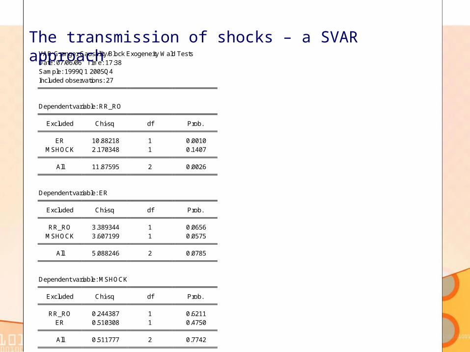
VAR Granger Causality/Block Exogeneity Wald Tests Date: 07/06/06 Time: 17:38 Sample: 1999Q1 2005Q4 Included observations: 27

Dependent variable: RR_RO Excluded Chi-sq df Prob. ER 10.88218 1 0.0010

MSHOCK 2.170348 1 0.1407 All 11.87595 2 0.0026

Dependent variable: ER Excluded Chi-sq df Prob. RR_RO 3.389344 1 0.0656

MSHOCK 3.607199 1 0.0575 All 5.088246 2 0.0785

Dependent variable: MSHOCK Excluded Chi-sq df Prob. RR_RO 0.244387 1 0.6211

ER 0.510308 1 0.4750 All 0.511777 2 0.7742


Concluding remarks

The monetary shocks are isolated by estimating a reaction function for the euro area. A more appropriate method to identify the policy shocks is to use the information set available at the moment the decision is made, i.e. survey data.

The empirical evidence does not support an impact of these shocks on the internal variables.- The number of observations used for the estimation may be inappropriate for

the analyses of monetary transmission, knowing that the monetary decisions affect the economy only with lags.

- For the major part of the analyzed period, Romania’s exchange rate regime was managed floating, but according to empirical findings and to IMF, it was a mixed regime in the form of sliding band. The theoretical results for the case of floating exchange rate may not hold if this assumption is not met.

- Moreover, the capital account has not been fully liberalized and the stages with the greatest impact on the balance of payments occurred in only in 2005. The financial openness is questionable before this period.

Concluding remarks

Not European business cycles and monetary innovations determine the internal economic indicators, but domestic economic and political developments.

- During transition period major internal disturbances affected the Romanian economy; these internal shocks include the effects of domestic political conflicts, economic and financial crises, domestic policy mistakes and so on.

- Apart from the obvious advantages incurred by the imminent accession, the unpredictable effect of the European monetary policy on the Romanian economic variables can trigger integration costs not dealt with so far.

Further research:- Alternative methods for identification of monetary policy shocks

(using the data-determined approach and the Blanchard and Quah decomposition).

- The reaction function for the ECB can be obtained by employing monthly data, using cubic splines on real GDP.

- In order to test the relevance of the theme it is useful to analyze the transmission of the identified monetary policy shocks in other countries except Romania, namely the new EU member countries. It can also be tested whether there is an asymmetry bween the effects of a negative and positive monetary shock.

[1] Beier, N., & Storgaard, P. 2006. Identifying monetary policy in a small open economy under fixed exchange rates. Danmarks Nationalbank Working Paper 36/2006

[2] Betts, C. and Devereux, M. 1999. The International Effects of Monetary and Fiscal Policy in a Two-country

Model. The University of British Columbia, Discussion Paper No. 99-10. [3] Bordo, M., & Murshid A.P. 2002. Globalization and Changing Patterns in the International Transmission of

Shocks in Financial Markets. NBER Working Papers 9019/2002 [4] Brooks, Chris. 2002. Introductory Econometrics for Finance. Cambridge: Cambridge University Press. [5] Brunner, A. 2000. On the Derivation of Monetary Policy Shocks: Should We Throw the VAR out with the

Bath Water? Journal of Money, Credit and Banking, 32(2):254-279, May 2000 [6] Carstensen, K. ,& Colavecchio, R. 2004. Did the Revision of the ECB Monetary Policy Strategy Affect the

Reaction Function? Kiel Working Paper No. 1221/2004 [7] Carstensen, K. (2003) Estimating the ECB policy reaction function, German Economic Review,

forthcoming. [8] Chari, V., Kehoe, P. and McGrattan, E. 1997. Monetary Shocks and Real Exchange Rates in Sticky Price

Models of International Business Cycles. NBER Working Papers No. 5876/1997 [9] Chari, V., Kehoe, P. and McGrattan, E. 2000. Can Sticky Price Models Generate Volatile and Persistent Real

Exchange Rates? NBER Working Papers No. 7869/2000

[10] Christiano, Lawrence J. 1996. Identification and the Liquidity Effect: A CaseStudy. Federal Reserve Bank of Chicago Economic Perspectives; 20(3): pp. 2-13, May June 1996

Selected references

[11] Christiano, L.J., Eichenbaum, M., & Evans, C. 1996. The Effect of Monetary Policy Shocks:

Evidence from the Flow of Funds. The Review of Economics and Statistics, 78(1):16-34.

[12] Christiano, L.J., Eichenbaum, M., & Evans, C. 1998. Monetary Policy Shocks: What Have We Learned and to What End? NBER Working Paper, 6400/1998

[13] Chu, J., & Ratti R., 1997. Effects of Unanticipated Monetary Policy on Aggregate Japanese Output:

The Role of Positive and Negative Shocks. The Canadian Journal of Economics, 30(3):722-741.

[14] Clarida, R., Gali, J., and Gertler, M. 1997, Monetary Policy Rules and Macroeconomic Stability: Evidence and Some Theory. NBER Working Paper, 6442/1998

[15] Clarida, R. 2001. The empirics of monetary policy rules in open economies. International Journal of

Finance & Economic. 6( 4): 315-323

[16] Corsetti, G. and Pesenti, P. 1997. Welfare and Macroeconomic Interdependence. NBER Working Paper 6307/1997

[17] Cushman, D.O.,& Zha, T. 1997., Identifying Monetary Policy in a Small Open Economy Under

Flexible Exchange Rates, Journal of Monetary Economics, 39(3): 433 - 448.

[18] Dees, S., Pesaran, H., Smith, V., & Mauro, F. 2005. Exploring the International Linkages of the Euro Area. A global VAR Analysis. ECB Working Paper, 568 / 2005

[19] Devereux, M. B., & Engel, C. 2003. Monetary Policy in the Open Economy Revisited: Price Setting

and Exchange-rate Flexibility. The Review of Economic Studies, 245(70): 765-782

[20] Eichenbaum, M., & Evans, C. 1995. Some Empirical Evidence on the Effects of Shocks to Monetary Policy on Exchange Rates. The Quarterly Journal of Economics, 110(4):975-1009

Selected references

[21] Enders, Walter. 2004. Applied Econometric Time Series. US: John Wiley & Sons Ltd.

[22] Engel, C. 2002. The Responsiveness of Consumer Prices to Exchange Rates And the Implications for

Exchange-Rate Policy: A Survey Of a Few Recent New Open-Economy Macro Models. NBER Working Papers 8725/2002

[23] Faust, J., J. H. Rogers and J. H. Wright. 2001. An empirical comparison of Bundesbank and ECB

monetary policy rules, Board of Governors of the Federal Reserve System, International Finance Discussion Paper 705.

[24] Faust, J., J. H. Rogers, Swanson, E. and J. H. Wright. 2003. Identifying the Effects of Monetary

Shocks on Exchange Rates Using High Frequency Data. NBER Working Papers No. 9660/2003

[25] Gali, J. 2002. Monetary Policy in the Early Years of EMU. mimeo, CREI, Universitat Pompeu Fabra.

[26] Genberg, H. 2005. External shocks, transmission mechanisms and deflation in Asia. BIS Working Papers, 187/2005

[27] Gerdesmeier, D. and B. Roffia. 2003. Empirical estimates of reaction functions for the Euro area,

ECB, Working Paper 206.

[28] Gerdesmeier, D. and B. Roffia. 2005. Taylor rules for the euro area: the issue of realtime data, Deutsche Bundesbank Discussion Paper Series 1: Studies of the Economic Research Centre No 37/2004.

[29] Gerlach, S. 2004. Interest Setting by the ECB: Words and Deeds, CEPR Discussion Paper No. 4775.

[30] Gerlach-Kristen, P. 2003. Interest rate reaction functions and the Taylor rule in the Euro area, ECB,

Working Paper 258.

[31] Hayashi, Fumio. 2000. Econometrics. Princeton: Princeton University Press.

Selected references

[32] Hayo, B., & Hofmann, B. 2005. Comparing Monetary Policy Reaction Functions: ECB versus

Bundesbank. Marburg Papers on Economics. No. 02-2005

[33] Obstfeld, M. & Rogoff, K. 1995. Exchange Rate Dynamics Redux. Journal of Political Economy 103, 624—660.

[34] Orphanides, A. 2001. Monetary policy rules based on realtime data, American Economic Review, 91,

964985.

[35] Sauer S. and J.E. Sturm. 2003. Using Taylor Rules to understand ECB monetary policy, CESifo working paper 1110.

[36] Surico, P. 2003. How does the ECB target inflation?, ECB Working Paper 229/2003.

[37] Svensson, L.O. and van Wijnbergen, S. 1989. Excess Capacity, Monopolistic Competition, and

International Transmission of Monetary Disturbances. The Economic Journal. 99(397): 785-805

Selected references

international transmission of monetary policy shocks the case of romanian economy

Documents

principal componentspc

economic variables

total imports

analysis of comovements

degree of financial

total variance

higher loading

romanian economythe