international trade: theory and evidence - queen's...
TRANSCRIPT
International Trade: Theory and Evidence
"... the Prebisch-Singer Thesis is now incorporated, both implicitly andexplicitly, in the advice given by the Bretton Woods Institutions to
developing countries." Hans Singer (1998)
Fall 2010
Huw Lloyd-Ellis () Econ239 Fall 2010 1 / 34

Growth of World Trade
Growth in world exports:
1960�68 7.3%1968�73 9.7%1973�80 3.3%1980�85 2.3%1985�90 4.5%1990�07 6.0%
LDC export growth:
,! rapid in Asia
,! highly variable in Latin America
,! slow in Africa.
Huw Lloyd-Ellis () Econ239 Fall 2009 2 / 34

- 10 -
Figure 1. Growth of Merchandise Exports, 1970-20001
100
600
1100
1600
2100
2600
1970 1975 1980 1985 1990 1995 2000
inde
x (1
980=
100)
World
Source: IMF World Economic Outlook (WEO).1 Excluding oil exports.
Least Developed Countries
Other Developing Countries
Sub-Saharan Africa
Figure 3. World: Product Composition of Merchandise Exports, 1965-98
0
10
20
30
40
50
60
70
80
90
100
1965 1970 1975 1980 1985 1990 1995 1998
perc
ent
Agriculture
Manufactures
Minerals
Source: GTAP database, version 5.
Figure 2. Developing Countries: Share of Exports Going to Other Developing Countries, 1965-98
0
5
10
15
20
25
30
35
40
45
1965 1970 1975 1980 1985 1990 1995 1998
perc
ent
MineralsAgricultureManufacturesTotal
Source: Global Trade Analysis Project (GTAP) database, version 5.
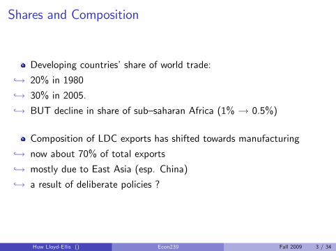
Shares and Composition
Developing countries�share of world trade:
,! 20% in 1980
,! 30% in 2005.
,! BUT decline in share of sub�saharan Africa (1% ! 0.5%)
Composition of LDC exports has shifted towards manufacturing
,! now about 70% of total exports
,! mostly due to East Asia (esp. China)
,! a result of deliberate policies ?
Huw Lloyd-Ellis () Econ239 Fall 2009 3 / 34

Table I.6
1948 1953 1963 1973 1983 1993 2003 2007
Value
World 59 84 157 579 1838 3675 7375 13619Share
World 100.0 100.0 100.0 100.0 100.0 100.0 100.0 100.0North America 28.1 24.8 19.9 17.3 16.8 18.0 15.8 13.6
United States 21.7 18.8 14.9 12.3 11.2 12.6 9.8 8.5Canada 5.5 5.2 4.3 4.6 4.2 4.0 3.7 3.1Mexico 0.9 0.7 0.6 0.4 1.4 1.4 2.2 2.0
South and Central America 11.3 9.7 6.4 4.3 4.4 3.0 3.0 3.7Brazil 2.0 1.8 0.9 1.1 1.2 1.0 1.0 1.2Argentina 2.8 1.3 0.9 0.6 0.4 0.4 0.4 0.4
Europe 35.1 39.4 47.8 50.9 43.5 45.4 45.9 42.4Germany a 1.4 5.3 9.3 11.6 9.2 10.3 10.2 9.7France 3.4 4.8 5.2 6.3 5.2 6.0 5.3 4.1Italy 11.3 9.0 7.8 5.1 4.0 4.6 4.1 3.6United Kingdom 1.8 1.8 3.2 3.8 5.0 4.9 4.1 3.2
Commonwealth of Independent States (CIS) b - - - - - 1.5 2.6 3.7Africa 7.3 6.5 5.7 4.8 4.5 2.5 2.4 3.1
South Africa c 2.0 1.6 1.5 1.0 1.0 0.7 0.5 0.5Middle East 2.0 2.7 3.2 4.1 6.8 3.5 4.1 5.6Asia 14.0 13.4 12.5 14.9 19.1 26.1 26.2 27.9
China 0.9 1.2 1.3 1.0 1.2 2.5 5.9 8.9Japan 0.4 1.5 3.5 6.4 8.0 9.9 6.4 5.2India 2.2 1.3 1.0 0.5 0.5 0.6 0.8 1.1Australia and New Zealand 3.7 3.2 2.4 2.1 1.4 1.4 1.2 1.2Six East Asian traders 3.4 3.0 2.4 3.4 5.8 9.7 9.6 9.3
Memorandum item: EU d - - 27.5 38.6 38.6 38.6 42.7 39.1USSR, former 2.2 3.5 4.6 3.7 5.0 - - -GATT/WTO Members e 62.8 69.6 75.0 84.1 78.4 89.4 94.3 94.1
Note: Between 1973 and 1983 and between 1993 and 2003 export shares were significantly influenced by oil price developments.
World merchandise exports by region and selected economy, 1948, 1953, 1963, 1973, 1983, 1993, 2003 and 2007
b Figures are significantly affected by i) changes in the country composition of the region and major adjustment in trade conversion factors between 1983 and 1993; and ii) including the mutual trade flows of the Baltic States and the CIS between 1993 and 2003.c Beginning with 1998, figures refer to South Africa only and no longer to the Southern African Customs Union.
e Membership as of the year stated.
a Figures refer to the Fed. Rep. of Germany from 1948 through 1983.
(Billion dollars and percentage)
d Figures refer to the EEC(6) in 1963, EC(9) in 1973, EC(10) in 1983, EU(12) in 1993, and EU(25) in 2003 and 2006.

- 12 -
Figure 4. Developing Countries: Composition of Merchandise Exports, 1965-98
0
10
20
30
40
50
60
70
80
90
100
1965 1970 1975 1980 1985 1990 1995 1998
perc
ent
Manufactures
Agriculture
Minerals
Source: GTAP database, version 5.
Figure 5. Share of Commerical Services in Total Exports of Goods and Services, 1980-97
5
10
15
20
25
1980 1981 1982 1983 1984 1985 1986 1987 1988 1989 1990 1991 1992 1993 1994 1995 1996 1997
perc
ent
Developing Countries
Sub-Saharan Africa
Industrial Countries
Source: World Bank; World Development Indicators (2001).
- 13 -
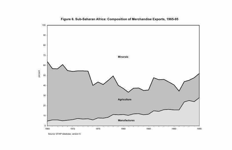
12. For regions such as SSA, there is concern about continuing dependence on commodity exports. An examination of changes in the composition of exports from SSA shows that, even for these countries, there has been a consistent but less dramatic upward trend in the share of manufactures exports (Figure 6). Nevertheless, three-fourths of SSA’s exports are still concentrated in primary commodities. While this explains part of the decline in SSA’s share of world trade, more than a third of the decline results from the loss of market shares in the goods that SSA produces and exports, rather than from the relatively slow growth of those commodity exports themselves (Figure 7).
Figure 6. Sub-Saharan Africa: Composition of Merchandise Exports, 1965-95
0
10
20
30
40
50
60
70
80
90
100
1965 1970 1975 1980 1985 1990 1995
pe
rce
nt
Manufactures
Agriculture
Minerals
Source: GTAP database, version 5.
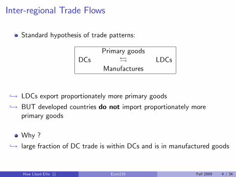
Inter-regional Trade Flows
Standard hypothesis of trade patterns:
DCsPrimary goods
�Manufactures
LDCs
,! LDCs export proportionately more primary goods
,! BUT developed countries do not import proportionately moreprimary goods
Why ?
,! large fraction of DC trade is within DCs and is in manufactured goods
Huw Lloyd-Ellis () Econ239 Fall 2009 4 / 34

Table I.4
(Billion dollars and percentage)
OriginNorth
America
South and Central America Europe CIS Africa Middle East Asia World
ValueWorld 2517 451 5956 397 355 483 3294 13619North America 951.2 130.7 328.7 12.4 27.3 50.1 352.1 1853.5South and Central America 151.3 122.0 105.6 6.4 13.7 9.1 80.2 499.2Europe 458.5 80.4 4243.6 189.0 147.7 152.9 433.7 5772.2Commonwealth of Independent States (CIS) 23.6 6.3 287.5 103.2 6.9 16.2 59.6 510.3Africa 91.9 14.6 167.5 0.9 40.5 10.5 80.9 424.1Middle East 83.9 4.4 108.3 4.8 27.5 93.4 397.3 759.9Asia 756.4 92.3 714.6 79.8 91.4 150.4 1889.8 3799.7Share of regional trade flows in each region's total merchandise exportsWorld 18.5 3.3 43.7 2.9 2.6 3.5 24.2 100.0North America 51.3 7.0 17.7 0.7 1.5 2.7 19.0 100.0South and Central America 30.3 24.4 21.2 1.3 2.7 1.8 16.1 100.0Europe 7.9 1.4 73.5 3.3 2.6 2.6 7.5 100.0Commonwealth of Independent States (CIS) 4.6 1.2 56.3 20.2 1.3 3.2 11.7 100.0Africa 21.7 3.4 39.5 0.2 9.5 2.5 19.1 100.0Middle East 11.0 0.6 14.3 0.6 3.6 12.3 52.3 100.0Asia 19.9 2.4 18.8 2.1 2.4 4.0 49.7 100.0Share of regional trade flows in world merchandise exportsWorld 18.5 3.3 43.7 2.9 2.6 3.5 24.2 100.0North America 7.0 1.0 2.4 0.1 0.2 0.4 2.6 13.6South and Central America 1.1 0.9 0.8 0.0 0.1 0.1 0.6 3.7Europe 3.4 0.6 31.2 1.4 1.1 1.1 3.2 42.4Commonwealth of Independent States (CIS) 0.2 0.0 2.1 0.8 0.1 0.1 0.4 3.7Africa 0.7 0.1 1.2 0.0 0.3 0.1 0.6 3.1Middle East 0.6 0.0 0.8 0.0 0.2 0.7 2.9 5.6Asia 5.6 0.7 5.2 0.6 0.7 1.1 13.9 27.9
Intra- and inter-regional merchandise trade, 2007
Destination

Actual World trade �ows
DCs Manufactures� DCs
Primary "# Manu. Primary "# Manu.
LDCs � LDCs
However, trade between LDCs has increased to about 10% of worldtrade
Huw Lloyd-Ellis () Econ239 Fall 2009 5 / 34
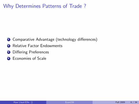
Why Determines Patterns of Trade ?
1 Comparative Advantage (technology di¤erences)2 Relative Factor Endowments3 Di¤ering Preferences4 Economies of Scale
Huw Lloyd-Ellis () Econ239 Fall 2009 6 / 34

1. Comparative Advantage � Ricardian Trade Theory
Example:
,! 2 countries: North and South,! 2 goods: Computers and Rice,! 1 factor: labour �600 workers each
,! perfect competition and labour mobility
Technological assumptions:
Labour One One sackRequired Computer of Ricein North 10 15in South 40 20
,! North has an absolute advantage in both goods,
,! but a comparative advantage in computers.
,! South has a comparative advantage in rice.
Huw Lloyd-Ellis () Econ239 Fall 2009 7 / 34
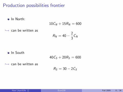
Production possibilities frontier
In North:10CN + 15RN = 600
,! can be written asRN = 40�
23CN
In South40CS + 20RS = 600
,! can be written asRS = 30� 2CS
Huw Lloyd-Ellis () Econ239 Fall 2009 8 / 34
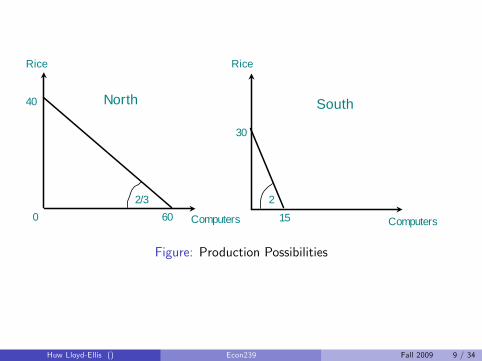
Rice Rice
Computers Computers
40
60
30
15
North South
2/3 20
Figure: Production Possibilities
Huw Lloyd-Ellis () Econ239 Fall 2009 9 / 34

Autarky
If both goods are consumed in North:
pNcpNr
=1015=23.
Why?
,! Competition )
pNc = 10wc and pNr = 15wr
If pNc10>
pNr15 , then wc > wr ) all workers �ow into computers
If pNc10 <
pNr15 , then wc < wr ) all workers �ow into rice
Huw Lloyd-Ellis () Econ239 Fall 2009 10 / 34

For both goods to be produced, we need
wc = wrpNc10
=pNr15
Similarly, if both goods are consumed in South:
pScpSr=4020= 2.
Huw Lloyd-Ellis () Econ239 Fall 2009 11 / 34

Free Trade
If both goods are going to be produced:
23<pcpr< 2.
Why ?
,! if pcpr <23 < 2, both countries specialize in rice
,! if pcpr > 2 >23 , both countries specialize in computers
If 23 <pcpr< 2,
,! North specializes in computers
,! South specializes in rice.
Huw Lloyd-Ellis () Econ239 Fall 2009 12 / 34

If it is cheaper to produce rice in North, why don�t people buy ricethere?
,! market wages adjust so that rice is not cheaper in the North.,! as we move from autarky to free trade
pNc " pNr #pSc # pSr "
,! so that
North :pNc10= wN >
pNr15) specialize in C
South :pSc40< wS =
pSr20) specialize in R
,! e¤ectively nulli�es North�s advantage in rice production.
Huw Lloyd-Ellis () Econ239 Fall 2009 13 / 34

Predictions of Ricardian Theory
Each country specializes in the production of the goods in which it hasa comparative advantage and exports them in return for other goods
All households in both countries are unambiguously better o¤ withfree trade than in autarky.
,! the wage in both countries rises
,! consumption possibilities lie outside the PPF
Caveats,! only one factor of production
,! labour is perfectly mobile across sectors
,! competitive markets
Huw Lloyd-Ellis () Econ239 Fall 2009 14 / 34

Rice Rice
Computers Computers
North South
0
ConsumptionConsumption
Production
pc/pr
pc/pr
X
M
X
M
Figure: Gains From Trade
Huw Lloyd-Ellis () Econ239 Fall 2009 15 / 34

2. Factor Endowments � Neoclassical Trade TheoryEli Heckscher and Bertil Ohlin
Example,! 2 countries: North and South,! 2 goods: Cars and Textiles,! 2 factors: Capital (K ) and Labour (L) � perfectly mobile
,! labour receives wage w and capital receives a rent r
,! identical preferences across countries
Cars
T exti les
Increas inguti l i ty
Huw Lloyd-Ellis () Econ239 Fall 2009 16 / 34

North is relatively well endowed with capital:
KN
LN>KS
LS
Car production is capital intensive and textile production is labourintensive.
,! given the same r/w . the optimal capital-labour ratio for cars exceedsthat for textiles:
K̂ iCL̂iC
>K̂ iTL̂iT
i = S , N
k iC > k iL i = S , N
How does the PPF look now?
Huw Lloyd-Ellis () Econ239 Fall 2009 17 / 34
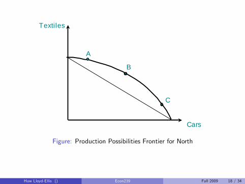
Textiles
Cars
A
B
C
Figure: Production Possibilities Frontier for North
Huw Lloyd-Ellis () Econ239 Fall 2009 18 / 34

Why is the PPF bowed out?
Shift towards more capital�intensive industry (A! B ! C )
,! drives up relative demand for capital
,! since relative supply is �xed, relative cost of capital, r/w , must rise
,! capital�labour ratios within each industry kC and kT fall in proportion
,! productivity of car production falls relative to that of textiles
,! for every unit of textiles given up, the gain in terms of cars declines
Huw Lloyd-Ellis () Econ239 Fall 2009 19 / 34
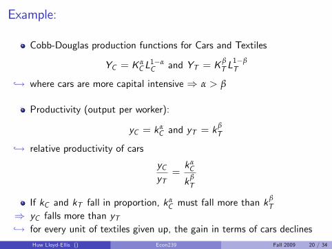
Example:
Cobb-Douglas production functions for Cars and Textiles
YC = KαCL
1�αC and YT = K
βT L
1�βT
,! where cars are more capital intensive ) α > β
Productivity (output per worker):
yC = kαC and yT = k
βT
,! relative productivity of cars
yCyT=kαC
kβT
If kC and kT fall in proportion, kαC must fall more than k
βT
) yC falls more than yT,! for every unit of textiles given up, the gain in terms of cars declines
Huw Lloyd-Ellis () Econ239 Fall 2009 20 / 34

Textiles
Cars
D
E
F
Figure: PPF for South
Huw Lloyd-Ellis () Econ239 Fall 2009 21 / 34

Textiles
Cars
C
pC/pTN N
P
Excess Supply
ExcessDemand
Figure: Disequilibrium in Autarky
Huw Lloyd-Ellis () Econ239 Fall 2009 22 / 34
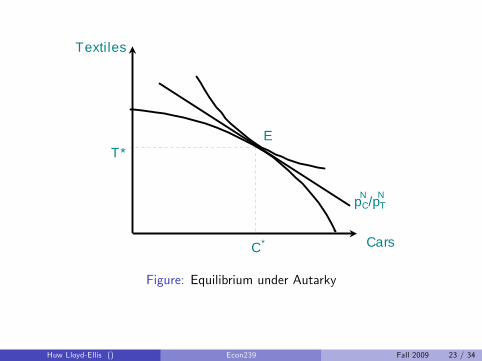
Textiles
Cars
pC/pTN N
ET*
C*
Figure: Equilibrium under Autarky
Huw Lloyd-Ellis () Econ239 Fall 2009 23 / 34

pC/pT
pC/pT
N N
S S
Figure: Autarky in North and South
Huw Lloyd-Ellis () Econ239 Fall 2009 24 / 34

pC/pT pC/pTNorth South
CN
PN
CS
PN
X
M X
M
Figure: Free Trade Equilibrium
Huw Lloyd-Ellis () Econ239 Fall 2009 25 / 34
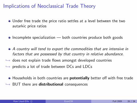
Implications of Neoclassical Trade Theory
Under free trade the price ratio settles at a level between the twoautarkic price ratios
Incomplete specialization � both countries produce both goods
A country will tend to export the commodities that are intensive infactors that are possessed by that country in relative abundance.
,! does not explain trade �ows amongst developed countries
,! predicts a lot of trade between DCs and LDCs
Households in both countries are potentially better o¤ with free trade,! BUT there are distributional consequences
Huw Lloyd-Ellis () Econ239 Fall 2009 26 / 34

3. Di¤erences in Preferences
Assume technologies and factor endowments are identical
How do preferences di¤er between LDCs and DCs ?
,! one hypothesis: DCs spend proportionately more on manufacturedgoods (luxuries)
,! i.e. as countries get richer, preferences biased away from primarygoods
,! drives down relative price of primary goods as DCs get richer
Huw Lloyd-Ellis () Econ239 Fall 2009 27 / 34

pC/pT
pC/pT
Textiles Textiles
Cars Cars
M
MX
X
Figure: Trade due to di¤erences in preferences
Huw Lloyd-Ellis () Econ239 Fall 2009 28 / 34

4. Economies of Scale
Trade allows concentration of production in some countries tomaximize the e¤ects of economies of scale
Example:,! 2 identical countries � East and West
,! 2 goods � ships and aircraft
,! declining average cost
Huw Lloyd-Ellis () Econ239 Fall 2009 29 / 34

Aircraft Ships
AC AC
$ $
A BC D
Autarky
Figure: Trade and Specialization with Economies of Scale
Huw Lloyd-Ellis () Econ239 Fall 2009 30 / 34
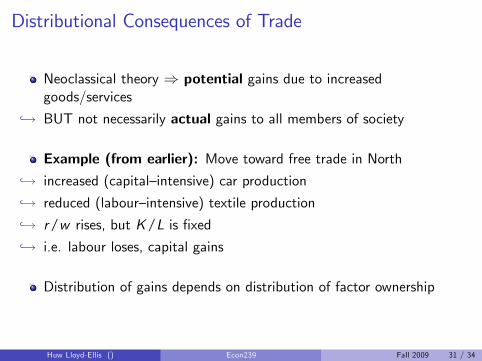
Distributional Consequences of Trade
Neoclassical theory ) potential gains due to increasedgoods/services
,! BUT not necessarily actual gains to all members of society
Example (from earlier): Move toward free trade in North,! increased (capital�intensive) car production
,! reduced (labour�intensive) textile production
,! r/w rises, but K/L is �xed,! i.e. labour loses, capital gains
Distribution of gains depends on distribution of factor ownership
Huw Lloyd-Ellis () Econ239 Fall 2009 31 / 34

Static vs. Dynamic Gains/Losses from Trade
Comparative advantage is a static concept,! but technologies and factor endowments change over time
LDCs could allow trade patterns to change as they accumulatephysical / human capital
,! �natural� shift from primary to manufacturing
,! BUT may get stuck as primary producer and never invest enough toget beyond this stage
Huw Lloyd-Ellis () Econ239 Fall 2009 32 / 34
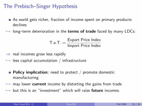
The Prebisch�Singer Hypothesis
As world gets richer, fraction of income spent on primary productsdeclines
,! long�term deterioration in the terms of trade faced by many LDCs:
T.o.T. =Export Price IndexImport Price Index
) real incomes grow less rapidly
,! less capital accumulation / infrastructure
Policy implication: need to protect / promote domesticmanufacturing
,! may lower current income by distorting the gains from trade
,! but this is an �investment�which will raise future incomes.
Huw Lloyd-Ellis () Econ239 Fall 2009 33 / 34

Does this hypothesis make any sense?
Not necessary that world demand will go against primary products
,! slow recovery from 60% decline in early 1980s
,! but recent rapid increase primary product prices (China, speculation?)
,! volatility a problem in itself
Policy implication assumes capital markets are not working properly
,! high future returns in manfacturing should induce investment �owinto it and away from primary production
BUT there are many market failures,! imperfect capital markets,! dynamic gains from investment may involve positive externalities) may justify government intervention in the form of trade policy.
Huw Lloyd-Ellis () Econ239 Fall 2009 34 / 34
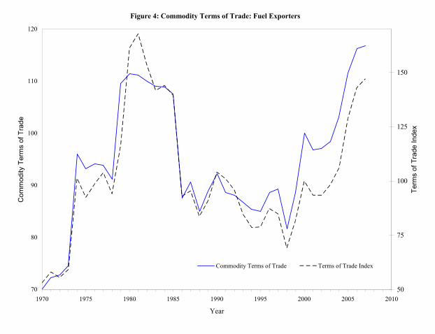
10
exporting countries, the qualitative differences among the indices are even larger, but not
surprisingly both indices display relatively little variation in absolute terms. In the next
section, we discuss the differences further, in the context of individual countries.
Figure 4: Commodity Terms of Trade: Fuel Exporters
70
80
90
100
110
120
1970 1975 1980 1985 1990 1995 2000 2005 2010
Year
Com
mod
ity T
erm
s of
Tra
de
50
75
100
125
150
Ter
ms
of T
rade
Ind
ex
Commodity Terms of Trade Terms of Trade Index
III. IDENTIFYING COMMODITY BOOMS AND BUSTS
The commodity terms of trade (CTOT) are now used to identify country-specific
booms and busts over the period 1970–2007. The dating procedure is an application of the
Bry-Boschan algorithm for dating business cycles and largely follows Cashin, McDermott,
and Scott (2002). It is based on finding turning points (peaks and troughs) in the country-
specific CTOT series. These turning points are determined using annual country-specific

11
Figure 5: Commodity Terms of Trade: Non-Fuel Commodity Exporters
95
100
105
110
115
1970 1975 1980 1985 1990 1995 2000 2005 2010
Year
Com
mod
ity T
erm
s of
Tra
de
90
110
130
150
170
190
Ter
ms
of T
rade
Ind
ex
Commodity Terms of Trade Terms of Trade Index
data (this implies that cycles can only be identified if they are not too short). For each
country, the procedure yields a set of upturns (trough-to-peak) and downturns (peak-to-
trough) in the CTOT, that is, a set of CTOT cycles.
Our focus, however, is on identifying large movements in the CTOT, since these are
most likely to be related to macroeconomic performance. Hence, for each cycle in the CTOT,
the duration and amplitude (that is, the cumulative change in the CTOT) from trough to peak
and from peak to trough are computed. Booms (respectively, busts) are then identified as
periods of increases (respectively, decreases) in the CTOT with amplitudes that fall into the
top (respectively, bottom) 10 percent of all such episodes across the sample. These cutoff
amplitudes imply that booms (respectively, busts) are defined as events with net commodity
trade gains (respectively, losses) in excess of 7 percent of GDP. This procedure