IZA DP No. 1590

International Migration:A Panel Data Analysis of Economicand Non-Economic Determinants

Anna Maria Mayda

DI

SC

US

SI

ON

P

AP

ER

S

ER

IE

S

Forschungsinstitut

zur Zukunft der Arbeit

Institute for the Study

of Labor

May 2005

International Migration:

A Panel Data Analysis of Economic and Non-Economic Determinants

Anna Maria Mayda Georgetown University

and IZA Bonn

Discussion Paper No. 1590 May 2005

IZA

P.O. Box 7240 53072 Bonn

Germany

Phone: +49-228-3894-0 Fax: +49-228-3894-180

Email: iza@iza.org

Any opinions expressed here are those of the author(s) and not those of the institute. Research disseminated by IZA may include views on policy, but the institute itself takes no institutional policy positions. The Institute for the Study of Labor (IZA) in Bonn is a local and virtual international research center and a place of communication between science, politics and business. IZA is an independent nonprofit company supported by Deutsche Post World Net. The center is associated with the University of Bonn and offers a stimulating research environment through its research networks, research support, and visitors and doctoral programs. IZA engages in (i) original and internationally competitive research in all fields of labor economics, (ii) development of policy concepts, and (iii) dissemination of research results and concepts to the interested public. IZA Discussion Papers often represent preliminary work and are circulated to encourage discussion. Citation of such a paper should account for its provisional character. A revised version may be available directly from the author.

IZA Discussion Paper No. 1590 May 2005

ABSTRACT

International Migration: A Panel Data Analysis of Economic and Non-Economic Determinants∗

In this paper I empirically investigate economic and non-economic determinants of migration inflows into fourteen OECD countries by country of origin, between 1980 and 1995. The annual panel data set used makes it possible to exploit both the time-series and cross-country variation in immigrant inflows. I focus on both supply and demand determinants of migration patterns and find results broadly consistent with the theoretical predictions of a standard international-migration model. Both first and second moments of the income distribution in the destination and origin countries shape international migration movements. In particular, I find evidence of robust and significant pull effects, that is the positive impact on immigrant inflows of improvements in the mean income opportunities in the host country. Inequality in the origin and destination economies affects the size of migration rates as predicted by Borjas (1987) selection model. Finally, among the non-economic determinants, I investigate the impact on emigration rates of geographical, cultural, and demographic factors as well as the role played by changes in destination countries’ migration policies. JEL Classification: F22 Keywords: international migration, push and pull factors, network effects Corresponding author: Anna Maria Mayda Department of Economics and School of Foreign Service Georgetown University Washington, DC 20057 USA Email: amm223@georgetown.edu

∗ I would like to thank Alberto Alesina, Elhanan Helpman, and Dani Rodrik for support and many insightful comments. For helpful suggestions, I am also grateful to Richard Adams, Marcos Chamon, Bryan Graham, Louise Grogan, Russell Hillberry, Rod Ludema, Maurice Schiff, Tara Watson, Jeffrey Williamson, and participants in the International Workshop at Harvard University, at the 2003 NEUDC Conference at Yale University, at the International Trade Commission Workshop, at the World Bank International Trade Seminar and at IZA Annual Migration Meeting. I am grateful for research assistance provided by Krishna Patel and Pramod Khadka. Finally, I would also like to thank the Center for International Development at Harvard University for making available office space. All errors remain mine.

1 Introduction

Do flows of international migrants respond to economic incentives, in spite of destinationcountries’ restrictive immigration policies? Which economic determinants affect internationalmigration flows? Do non-economic variables - such as geographical, cultural and demographicfactors - shape cross-country immigration patterns? What role do host countries’ restrictiveimmigration policies play? Are network effects at work? In this paper, I address thesequestions using a yearly panel data set that allows me to exploit both the time-series andcross-country variation in international immigrant flows.Cross-country migration patterns vary considerably over time, and across destination

and origin countries (see Appendix 2). Some OECD countries have experienced a decreasein the size of the annual immigrant inflow between 1980 and 1995.1 Over the same years,the number of immigrants per year has increased in several other OECD countries.2 Thepercentage change of the yearly immigrant inflow in this period ranges between negative 42%(in Japan) and positive 48% (in Canada) (OECD 1997). For all destinations, such changesare anything but monotonic (see Figure 3). The variation in terms of origin countries isremarkable as well.Both economic and non-economic factors are likely to influence the size, origin, and

destination of labor movements at each point in time and contribute to the variation observedin the data. While clearly it is important to understand the driving forces behind recentinternational migration patterns, a limited amount of empirical research has been devotedto this topic, perhaps due to past unavailability of cross-country data on migration.In this paper, I empirically investigate economic and non-economic determinants of bi-

lateral immigrant flows, across destination and origin countries.3 I first derive testable pre-dictions about the main factors affecting international migration, using a simple theoreticalframework. My model focuses on both supply and demand determinants of immigrationpatterns. Next, I empirically relate bilateral migrant flows (normalized by origin country’spopulation) to the economic, geographical, cultural and demographic determinants suggestedby the theory. The explanatory variables I identify are mean income opportunities in thesource and destination country, their relative income inequality, the distance and commonborders between the two countries, their colonial links and common languages, and theimmigration-policy legislation in the host country. The age structure of the origin country’spopulation and network effects are additional determinants suggested by the theoreticalmodel (Clark, Hatton and Williamson 2002).To analyze migration patterns across countries, I use yearly data on immigrant inflows

1For example, Australia, France, Japan, Netherlands, and the United Kingdom.2For example, in Belgium, Canada, Denmark, Germany, Luxembourg, Norway, Sweden, Switzerland, and

the United States.3While I distinguish between "economic" and "non-economic" determinants, there is an economic ratio-

nale behind the impact of both sets of variables on migration flows.

2

into fourteen OECD countries by country of origin, between 1980 and 1995. The source ofthis data is the International Migration Statistics for OECD countries (OECD 1997), basedon the OECD’s Continuous Reporting System on Migration (SOPEMI).My empirical analysis both delivers estimates broadly consistent with the theoretical

predictions of a standard international-migration model and generates empirical puzzles.Among the economic determinants, I investigate the effect on international immigrant

flows of both first and second moments of the income distributions in the destination andorigin countries.4 I find that pull factors - that is, improvements in the mean income op-portunities in the destination country - significantly increase the size of emigration rates.This result is very robust to changes in the specification of the empirical model. In addition,both absolute and relative pull factors matter. The emigration rate to a given destination isestimated to be an increasing function of that country’s per worker GDP and a decreasingfunction of the average per worker GDP of all the other host countries in the sample5 (eachweighted by the inverse of distance from the origin country).Positive and significant pull effects may appear, at first sight, inconsistent with restrictive

immigration policies of several destination countries in the sample.6 From a theoreticalpoint of view, the impact of pull (and push) factors is a function of whether immigration isquantity-constrained. If immigration quotas are binding in the host country, pull (and push)factors should have no effect. However, my results show that pull effects matter, in spite ofimmigration restrictions of most destination countries in the sample. One interpretation ofthis finding is that the estimated coefficient simply captures an average effect, across countrypairs characterized by different immigration-policy arrangements: as long as immigrationconstraints are not binding for each country pair, this average effect should - according to thetheory - be positive. I find evidence consistent with this interpretation when I differentiatethe effect of pull and push factors according to each host country’s restrictiveness towardsimmigrants. In particular, I interact mean income opportunities in, respectively, the hostand source country with an indicator variable of changes in destination countries’ migrationpolicies. I find that, when immigration laws become less restrictive in a host country, theeffect of pull (push) factors in that country turns more positive (negative).Another explanation of my result - that is, positive and significant pull effects - is that

even countries with binding official immigration quotas often accept unwanted (legal) im-migration. Restrictive immigration policies are often characterized by loopholes, that leaveroom for potential migrants to take advantage of economic incentives. For example, immi-gration to Western European countries still took place after the late Seventies, despite theofficial closed-door policy (Joppke 1998). Family-reunification policies are thought to be one

4The income distributions of interest are the ones which characterize the origin country’s population ineach location.

5Since the host countries in the sample include the great majority of destinations of immigrants in theworld, it is not overly restrictive to focus on them.

6The data set I use only covers legal migration.

3

reason behind continuing migration inflows.7

Controlling for destination and origin countries’ fixed effects, the sign of the impact ofpush factors - that is, declining levels of per worker GDP in the origin country - is seldomconsistent with the theoretical predictions of the basic model. In those cases, the size of theeffect is smaller than for pull factors and is almost always insignificant. This is surprisinggiven that, in the basic model, push and pull factors have similar-sized effects (with oppositesigns). An explanation of my result is that the impact of income opportunities in the origincountry is likely to be affected by poverty constraints, due to fixed costs of migration andcredit-market imperfections (Schiff 1998 and Yang 2003). Lower levels of per worker GDP inthe source country both strengthen incentives to leave and make it more difficult to overcomepoverty constraints. In the empirical analysis I find (weak) evidence that my result on pushfactors is driven by poverty constraints in the origin country.Yet another interpretation of my findings is that positive and significant pull effects and

insignificant push effects are explained by the demand side of international migration (i.e.,migration policies), and not by the supply side as is often assumed in the previous literature.The theoretical model makes the assumption that migration quotas are exogenous. In real-ity changes in mean income opportunities in the destination country affect both migrants’incentive to move and the political process behind the formation of migration policies. Ifmigration quotas are binding, only the latter channel will be at work and the determinantson the supply side won’t have any effect.8

Inequality in the source and host economies is related to the size of emigration ratesas predicted by Borjas (1987) selection model. An increase in the origin country’s relativeinequality has a non-monotonic effect on the size of the emigration rate: the impact isestimated to be positive if there is positive selection, negative if there is negative selection.Next, I investigate the role played by geographical, cultural and demographic factors.

Among the variables affecting the costs of migration, distance between destination and ori-gin country appears to be of considerable importance. Its effect is negative, significantand steady across specifications. On the other hand, controlling for destination and origincountries’ fixed effects, I don’t find evidence that cultural variables play a significant role.Demographics - in particular, the share of the origin country’s population who is young -shapes bilateral flows as predicted by the theory.Finally, I empirically investigate the importance of network effects. Since immigrants are

likely to receive support from compatriots already established in the host country, they willhave an incentive to choose destinations with larger communities of fellow citizens. Network

7Another channel of entry of immigrants in countries with official closed-door policy is asylum-seekerslaws. Joppke (1998) writes about Germany’s experience (p.285): “Since the recruitment stop of 1973, thechain migration of families of guest workers was (next to aylum) one of the two major avenues of continuingmigration flows to Germany, in patent contradiction to the official no-immigration policy.”

8Notice that a deeper analysis of the demand side of international migration is outside the scope of thispaper and it’s an interesting direction of future research.

4

effects imply that bilateral migration flows are highly correlated over time, which is whatI find in my analysis. However, the interpretation of this result is ambiguous as it couldbe driven by either supply factors (that is, network effects) or by demand factors (familyreunification policies, for example).The empirical literature on the determinants of migration includes a number of works,

some of which date back to the nineteenth century (Ravenstein 1885). More recently, Clark,Hatton and Williamson (2002) and Karemera, Oguledo and Davis (2000) both focus on thefundamentals explaining immigrant inflows into the United States by country of origin inthe last decades. Helliwell (1997 and 1998) sheds light on factors affecting labor movementsin his investigation of the magnitude of immigration border effects, using data on Canadianinterprovincial, US interstate and US-Canada cross-border immigration.The contribution of this paper to the literature is threefold. First, my work is the first

one I am aware of to use the OECD (1997) data on international migration to systematicallyinvestigate the economic and non-economic determinants of international flows of migrants.Previous works have either used country cross-sections (Borjas 1987 and Yang 1995, forexample), or have focused on a single destination country over time (Borjas and Bratsberg1996, Clark, Hatton and Williamson 2002, and Karemera, Oguledo and Davis 2000, forexample) or a single origin country over time (for example, Yang 2003).9 By extending thefocus of the analysis to a multitude of origin and destination countries and taking advantageof both the time-series and cross-country variation in the data, I can test the robustness andbroader validity of the results found in the previous literature.10

Second, this paper carefully reviews and proposes solutions to various econometric issuesthat arise in the empirical analysis, such as endogeneity and reverse causality. Some of theseeconometric complications have not been addressed in the previous literature. Finally, thispaper puts greater emphasis than previous works on the demand side of international migra-tion, i.e. destination countries’ migration policies. This change of perspective is important,given restrictive immigrant policies in the great majority of host countries.The framework used in this work to study migration flows is related to the gravity model

of trade, which is used to analyze bilateral trade flows across countries.11 As a matter of fact,I use several variables that appear frequently in the trade gravity literature (distance, border,common language, and colony). There also exists a gravity model of immigration, developedin the geography literature and sometimes used in economics papers. However, the empirical

9From a methodological point of view, the paper most related to mine is Clark, Hatton, and Williamson(2002).10Since I began my work on international migration, I have become aware of another related, but indepen-

dent paper analyzing cross-country migration patterns: Pedersen, Pytlikova, and Smith (2004). This paperuses another data set to explore the determinants of international migration.11A number of works empirically analyzes trade flows within this setting (Helpman 1987 and Hummels

and Levinsohn 1995). The same type of framework is used to explain bilateral cross-border equity flowsacross countries (Portes and Rey 2002) as well as FDI flows (Brenton et al. 1999, Frankel and Wei 1996,and Mody, Razin and Sadka 2002).

5

specification I use, suggested by economic theory, differs in part from the standard equationestimated by geographers.12

The rest of the paper is organized as follows. Section 2 presents a simple model ofinternational migration. In Section 3 I describe the data sets used in the empirical part,while in Section 4 I discuss the estimating equations and some econometric issues thatcomplicate the analysis. Finally, Section 5 presents the main empirical results and Section6 concludes.

2 Theoretical framework

Both supply and demand factors determine international migration flows. Migrants’ deci-sion to move, according to economic and non-economic incentives, shape the supply sideof labour movements. The host country’s immigration policy represents the demand side,i.e. the demand for immigrants in the destination country. The latter one, in turn, canbe thought of as the outcome of a political-economy model in which individual attitudestoward immigrants, interest-groups pressure, policy-makers preferences and the institutionalstructure of government interact with each other and give rise to a final immigration-policyoutcome (Rodrik 1995, Facchini and Willmann 2004, Mayda 2003).The theoretical framework used in this paper is closely related to the previous literature.

The main difference is the greater emphasis in my model on demand factors, i.e. destinationcountries’ immigration policy. I will consider a world with two economies: country 0, which isthe country of origin of immigrant flows and country 1, which is the country of destination.I will first focus on the supply side of immigration, that is migrants’ decision to move.In particular, I will look at the probability that an individual chosen randomly from thepopulation of country 0 will migrate to country 1.In each country, wages are a function of the individual skill level (si). In the origin

country, the wage of individual i equals:

w0i = α0 + θ0 · si + disturbance0i, (1)

while in the country of destination:

w1i = α1 + θ1 · si + disturbance1i, (2)

where the two disturbances have both zero means over the origin country’s population.Since in the empirical analysis I will use aggregate data, I need to rewrite individual i’s wages

12The standard equation estimated by geographers looks as follows (Gallup 1997): flowij ∝ PiPjdist2ij

. As

Helliwell (1997) points out, there is still a contrast between economic and gravity explanations of immigrantflows.

6

in the two locations as a function of the mean wages of the origin country’s population athome and abroad respectively:13

w0i = µ0 + v0i, where v0i ∼ N(0, σ20), (3)

w1i = µ01 + v1i, where v1i ∼ N(0, σ21), (4)

where the correlation coefficient between v0i and v1i equals ρ01.Notice that µ0 equals α0 + θ0 · s0 and µ01 equals α1 + θ1 · s0, where s0 is the mean skill

level of the origin country’s population. The parameter µ01 is likely to be different from µ1,the mean wage in country 1 of the destination country’s population: µ1 = α1+ θ1 · s1, wheres1 represents the mean skill level of the destination country’s population (Borjas 1999a, andClark, Hatton and Williamson 2002). This point will become relevant below, in the empiricalanalysis.I assume that each individual has Cobb Douglas preferences for the two goods produced

in the world (x1 and x2):

U(x1, x2) = Ax1−δ1 xδ2, 0 < δ < 1, A > 0, (5)

which implies an indirect utility (function) from having an income y given by:14

v(p1, p2; y) = A(p1, p2) · y. (6)

I assume that each country is a small open economy characterized by free trade with therest of the world:15 therefore goods’ prices p1 and p2 are given and equal - and A(p1, p2) alsodoes not vary - across countries.16 An individual in country 0 will migrate to country 1 ifthe utility of moving is greater than the utility of staying at home i.e., given the assumptionsabove, if the expected income in the destination country net of migration costs is greaterthan the expected income in the origin country. Following the literature (for example, Borjas1999a, and Clark, Hatton and Williamson 2002), I can define an index Ii that measures thenet benefit of moving relative to staying at home for a risk-neutral individual i:

Ii = η01 · (w1i − w0i − Ci) + (1− η01) · (−w0i − Ci), (7)

⇒ Ii = η01 · w1i − w0i − Ci, (8)

13More in general, in (3) and (4), w0i and w1i are rewritten as a function of first and second moments ofthe income distribution of the origin country’s population at home and abroad respectively.14In the following expression: A(p1, p2) = A( 1−δp1

)1−δ( δp2 )δ.

15Given free trade, what explains differences in rates of return to labor across countries? The answer isthat the conditions for factor price equalization are not satisfied: for example, if international productivitydifferences exist, as in Trefler (1993), then only adjusted factor-price-equalization holds.16In the empirical analysis I adjust for international differences in goods’ prices, using PPP income levels.

7

where η01 is the probability that the migrant from country 0 will be allowed to stay incountry 1, w0i and w1i are respectively the wage in the origin and destination country, andCi = µC + vCi , with vCi ∼ N(0, σ2C), represents the level of individual migration costs.

17 Thecorrelation coefficients between vCi and (v0i, v1i) are equal to (ρ0C , ρ1C).This model focuses on labor mobility. Migration allows an individual to take advantage

of differences in rates of return to labor across countries. Migrants may own capital, eitherat home or in the destination country, but their capital income opportunities are assumed tobe independent of their residence. That is why the index Ii does not include a capital-incometerm.18

In addition, the implicit assumption in (8) is that, if the migrant is not allowed to stayin the destination country, he still incurs the migration costs Ci and gives up the home wagew0i. In other words, the individual moves to the host country before knowing whether hewill be able to stay (for a longer period of time) and gain the income w1i.19 The immigrantfrom country 0 may not be allowed to stay in country 1 because of quotas due to a restrictiveimmigration policy, as is explained below.The probability that an individual chosen randomly from the population of the origin

country will migrate from country 0 to country 1 equals:

P = Pr[Ii > 0] = Pr[η01 · (µ01 + v1i)− (µ0 + v0i)− (µC + vCi ) > 0], (9)

which can be rewritten as:

P = 1− Φ(z), (10)

where z = − (η01·µ01−µ0−µC)σv

, σv is the standard deviation of (η01 ·v1i−v0i−vCi ), and Φ(·) isthe cumulative distribution function of a standard normal.20 The probability of emigrationfrom country 0 to country 1 in (10) is approximated by the supply emigration rate IS01

P0, i.e.

the emigration rate on the supply side of the migration model.Consider now a situation in which the destination country’s immigration policy implies

either explicit or implicit quantity constraints for immigrants coming from each origin coun-try.21 Let ID01 represent the maximum number of migrants from country 0 allowed each period

17I assume that each individual knows the wage levels w1i and w0i he would get in each location, themigration costs Ci and the probability η01. Notice that, while each individual takes the probability η01 asgiven, this probability is endogenously determined in the model.18In other words, capital is internationally mobile. The migrant can own capital in the origin and desti-

nation country and receive income from it, no matter where he resides.19This assumption is consistent with the evidence that immigrants often arrive to a destination country

with tourist or student visas with the hope of being able to stay.20In particular, σ2v = (η

201σ

21 + σ20 + σ2C − 2η01ρ01σ0σ1 − 2η01ρ1Cσ1σC + 2ρ0Cσ0σC).

21My model differs from previous ones in the literature in the way it analyzes the impact of quantity re-strictions induced by immigration policy. Clark, Hatton, and Williamson (2002) and Hatton and Williamson(2002) model immigration policy as affecting the level Ci of migration costs.

8

into country 1. These immigration quotas may or may not be binding.What we can observe in the data is the actual emigration rate I01

P0, i.e. the number of

immigrants from country 0 to country 1, divided by the population of country 0. Only in theabsence of binding immigration quotas does the actual emigration rate I01

P0equal the supply

emigration rate IS01P0. In the presence of binding quantity-constraints, I01

P0will be less than IS01

P0.

That is, the actual emigration rate is equal to the minimum between IS01P0and ID01

P0:

I01P0= min(

IS01P0,ID01P0), (11)

where the immigration quota ID01 represents country 1’s demand for immigrants fromcountry 0, which is a function of country 1’s immigration policy. The heavy lines in Figure 1give the actual emigration rate as a function of µ01 and µh, h = 0, C. In this paper I assumethat ID01 is exogenous, thus it is not affected by µ

01 neither by µh, h = 0, C.

22 This is a strongassumption that will be questioned in the interpretation of the empirical results.I assume that the probability η01 - that the migrant from country 0 will be allowed to

stay in country 1 - is equal to min{1, ID01P0·P } (the number of people, from country 0 to country

1, who are allowed in, divided by the number of those who try to get in).Given (10) and (11), it is possible to derive testable predictions for the impact of µ01, µ0,

and µC on the actual emigration rate from country 0 to country 1:23

d( I01P0)

dµ01= {

φ(z)σv

> 0, if IS01P0

<ID01P0;

0, if IS01P0≥ ID01

P0

(12)

d( I01P0)

dµh= { −

φ(z)σv

< 0, if IS01P0≤ ID01

P0;

0, if IS01P0

>ID01P0

(13)

where φ(·) is the density function of a standard normal and h = 0, C. The comparative-static results in (12) show the effect of pull factors - that is, improvements of the mean incomeopportunities in the destination country - according to whether the immigration quotas arebinding or not. Pull effects are positive and strongest when restrictions are not bindingneither ex-ante nor ex-post, they are positive but smaller in size when the quota is bindingex-post but not ex-ante and, finally, they are equal to zero in a quantity-constrained world.

22Alternatively, ID01 can be explicitly modeled within a political-economy framework. In that case, theimmigration quotas are likely to depend on the capital-labor ratio of the median voter (see Benhabib 1996),on the size of past immigration flows from the same origin country, both because of family-reunificationpolicies and because of pro-immigration votes of naturalized immigrants (Ortega 2004), and on the extent ofpolitical organization of various interest groups (Grossman and Helpman 1994 and Facchini and Willmann2004).23The total differential of P equals:dP = φ(z)

σvd(η01µ

01 − µ0 − µC) + φ(z) (η01µ

01 − µ0 − µC)(− 1

σ2v)dσv.

9

A parallel interpretation explains the comparative-static results in (13), which describe pusheffects (changes of µ0, that is mean income opportunities in the origin country) and theimpact of mean migration costs (changes of µC), according to the immigration-policy regime.Thus, according to this simple model, pull and push factors have either similar-sized

effects (with opposite signs), when quotas are not binding, or they both have no effect onemigration rates, when quotas are binding. In the empirical analysis I will not be able tocontrol for whether a country-pair/year observation is characterized by binding migrationquotas or not (since I do not have data on ID01). Therefore I will estimate an average effectacross pairs of countries characterized by either one of them. However, I will be able touse information on changes of ID01. I should find that pull (push) effects are more positive(negative) than average, for a given destination country, if that host country’s migrationpolicy becomes less restrictive.24

Focusing for simplicity on the region where immigration quotas are not binding, it isstraightforward to derive predictions for the impact on I01

P0of the second moments of the

income distributions of the origin country’s population, at home and abroad respectively. Inparticular, assuming that σC = 0, we obtain the following expressions (where k < 0):25

d( I01P0)

dσ1= k · (η01µ01 − µ0 − µC) · (σ1 − ρ01σ0), (14)

d( I01P0)

dσ0= k · (η01µ01 − µ0 − µC) · (σ0 − ρ01σ1). (15)

In my discussion I will assume that (η01µ01−µ0−µC) > 0 so that, based on first-moments

considerations, on average immigrants have an incentive to migrate. The results in (14) and(15) imply that, if σ0

σ1< 1 and ρ01 is sufficiently high (ρ01 >

σ0σ1), then dσ0 > 0 or dσ1 < 0

(i.e., an increase in the relative inequality σ0σ1) will increase the emigration rate. The intuition

about this result is straightforward. Given that income inequality in the origin country islower than in the destination country (σ0

σ1< 1) and that ρ01 is sufficiently high, this is a

situation with positive selection of immigrants from country 0 to country 1 (Borjas 1987):migrants are selected from the upper tail of the income distribution at home and end up inthe upper tail of the income distribution abroad (in both cases, the relevant distribution is theorigin country’s population one). For example, consider potential migrants from Portugal tothe United States (Figure 2). Given that income inequality is lower in Portugal than in theU.S. and assuming that ρ01 is sufficiently high, among Portuguese workers it’s the better-off

24The reason is that, with higher ID01, the range of µ01 (µ0) for which the effect is strictly positive (negative)

is wider.25Formulas (14) and (15) are based on the expression for dP in footnote 22 (given that immigration

quotas are not binding, then I01P0= P ). If quotas are not binding (η01 = 1), assuming that σC = 0, then:

dσv = [σ21 + σ20 − 2ρ01σ0σ1]−

12 [(σ1 − ρ01σ0)dσ1 + (σ0 − ρ01σ1)dσ0 − σ0σ1dρ01]. Notice that, in formula (14)

and (15), k = φ(z)(σ21 + σ20 − 2ρ01σ0σ1)−12 (− 1

σ2v) < 0.

10

who have an incentive to migrate while those at the lower tail of the income curve have anincentive to stay. The reason is that the probability of both very high and very low incomesis higher in the U.S. than in Portugal. An increase in income inequality in Portugal willmake individuals at the bottom of the income distribution relatively worse-off at home andwill increase their incentive to leave.Similarly, if σ0

σ1> 1 and ρ01 is sufficiently high (ρ01 >

σ1σ0), then dσ0 > 0 or dσ1 < 0 (i.e., an

increase in the relative inequality σ0σ1) will decrease the emigration rate. Given that income is

more dispersed at home than abroad, this is the case of negative selection of immigrants fromcountry 0 to country 1 (Borjas 1987): migrants are selected from the lower tail of the incomedistribution at home and end up in the lower tail of the income distribution abroad. Anexample of this situation is migration from Brazil to the U.S., given that income inequalityin the latter is lower than in the former (Figure 2). An increase in income inequality inBrazil will lower the emigration rate because those who were not migrating beforehand, thebetter-off, will have even less incentive to do so afterwards.Notice that, in a way similar to the impact of first moments, the effect of second moments

will be affected by whether immigration quotas are binding or not.Finally, a few extensions of this simple theoretical framework deliver interesting predic-

tions that I will discuss and investigate in the empirical section.

3 Data

In this paper, I combine an international panel data set on bilateral immigration flows withadditional macroeconomic and non-economic data on the origin and destination country ofeach immigrant flow. Data on immigration comes from the International Migration Statistics(IMS) data set for OECD countries (OECD 1997), which contains information on immigrantflows by country of origin, based on the OECD’s Continuous Reporting System on Migration(SOPEMI).26 Population registers and residence and work permits are the main sources ofthese statistics. In particular, I use data on yearly immigrant inflows into fourteen OECDcountries by country of origin, in the period 1980-1995. Appendix 2, at the end of the paper,presents summary statistics on immigrant inflows by host and source country, averaged overthe years 1980-1995 (see also Figure 3).Appendix 3 shows that the disaggregate (i.e., by country of origin) IMS statistics on

migrant flows don’t add up to 100% of the total flow into each destination country. Thepercentage of the total immigrant inflow covered by the disaggregate data ranges between45% (Belgium) and 84% (United States). Put differently, the data set includes zero flows incorrespondence of some country pairs (immigrant inflows from Italy to the United States,for example). Some of these observations correspond to truly zero flows, while others arelikely to correspond to very small flows. If the latter observations are recorded as zeros in

26Note that the IMS data does not cover illegal immigration.

11

the disaggregate data set, there will be a discrepancy between total flows and the sum offlows by origin country. In the empirical analysis I will keep zero-flows observations in thedata set.27 I will also investigate the robustness of my results using a Tobit model.28

Summary statistics and data sources of each variable used in the empirical model aredocumented in Appendix 1. Data on macroeconomic variables comes from various sources:the 2001World Development Indicators (World Bank 2001), the PennWorld Tables (versions5.6 and 6.1), and the World Bank’s Global Development Network Growth Database, MacroTime Series (Easterly and Sewadeh 2002). Geographical and cultural information, such ason great-circle distance, land border, common language, and colonial ties, comes from Glickand Rose’s (2001) data set on gravity-model variables. I also use statistics on the averagenumber of schooling years in the total population (over age 15) from Barro and Lee’s (2000)data set.29 Data on Gini coefficients of destination and origin countries, used to constructthe origin country’s relative inequality variable, comes from Deininger and Squire (1996)data set (only high-quality observations were used). Finally, information on origin countries’share of young population comes from the United Nations.A separate Appendix to the paper documents the main characteristics of the migration

policies of the destination countries in the sample and the timing (after 1980) of changes intheir legislations (Mayda and Patel, 2004).30 A data set of destination countries’ migration-policy changes, between 1980 and 1995, was constructed on the basis of the information inthis Appendix and used in the empirical analysis.

4 Empirical model

The theoretical framework in Section 2 suggests an empirical specification characterized bythe emigration rate as the dependent variable and, among the explanatory variables, themean wage of the origin country’s population in, respectively, the origin and destinationcountries. As approximations for the latter two variables, I use the (log) level of per workerGDP, PPP-adjusted (constant 1996 international dollars) in the two countries.31 Based onthe basic model, I expect pull effects to be positive on average and push effects to be negativeon average.Another determinant of bilateral immigration flows implied by the model of Section 2

is the distance between the two locations, which affects migration costs Ci. The further

27The results don’t change when I drop zero observations (see previous version of this paper).28See regression (4), Table 4.29Since this panel only contains data at five-year intervals (in the period I consider, the years covered are

1980, 1985, 1990, 1995), I linearly extrapolate figures for the in-between years (by assigning one fifth of thefive-year change in the variable to each year).30The Appendix can be found in my website.31Per worker GDP is not a direct measure of the mean wage of the origin country’s population at home

and abroad. See below for robustness checks related to this point.

12

away the two countries are, the higher the monetary travel costs for the initial move, aswell as for visits back home. Remote destinations may also discourage migration becausethey require longer travel time and thus higher foregone earnings. Another explanationas to why distance may negatively affect migration is that it is more costly to acquireinformation ex-ante about far-away countries (Greenwood 1997 and Lucas 2000). I introduceadditional variables that affect the level of migration costs Ci. A common land border islikely to encourage migration flows, since land travel is usually less expensive than air travel.Linguistic and cultural similarity are also likely to reduce the magnitude of migration costs,for example by improving the transferability of individual skill from one place to the other.Past colonial relationships should increase emigration rates, to the extent that they translateinto similar institutions and stronger political ties between the two countries, thus decreasingthe level of migration costs Ci.In a cross-country analysis, such as in this paper, unobserved country-specific effects

could result in biased estimates. For example, I may estimate a positive coefficient on thedestination country’s per worker GDP. Based on this result, it is not clear whether immi-grants go to countries with higher wages or, alternatively, whether countries with higherwages have other features that attract immigrants. Along the same lines, a negative coef-ficient on income at home leaves open the question of whether immigrants leave countrieswith lower wages or, alternatively, whether countries with lower wages have certain charac-teristics that push immigrants to leave. To (partly) get around this problem, I exploit thepanel structure of the data set and I introduce dummy variables for both destination andorigin countries. This allows me to control for unobserved country-specific effects which areadditive and time-invariant. All specifications in Tables 1, 4, 5, and 6 include destination andorigin countries’ fixed effects and have robust standard errors clustered by country pair, toaddress heteroscedasticity and allow for correlation over time of country-pair observations.32

Notice that destination country fixed effects allow me to control for features of destinationcountries’ immigration policy which don’t change over time and are common across origincountries. In order to capture the effect of changes in destination countries’ migration poli-cies, I introduce two interaction terms of an indicator variable of such changes with pull andpush factors, respectively. According to the theory, if the migration policy of a destinationcountry becomes less restrictive, the effect of pull (push) factors should turn more positive(negative).Finally, I introduce the share of the origin country’s population who is young (between 15

and 29 years old) as a demographic determinant of migration flows. Consider an extensionof the basic model in Section 2 to a multi-period setting. In this set-up, the individual caresnot only about current wage differentials net of moving costs, but about future ones too. AsClark, Hatton, and Williamson (2002) point out, this implies that a potential migrant fromcountry 0 will have a bigger incentive to migrate the younger he is, as the present discounted

32Most specifications in the tables include separate dummy variables for destination and origin countries,while the remaining regressions control for country-pair fixed effects.

13

value of net benefits will be higher the more extended the length of the remaining work lifetime (for positive Ii in each year). We would then expect the share of young population inthe origin country to increase the emigration rate out of that country.The basic empirical specification thus looks as follows:

flowijtPit

= β + β0pwgdpit−1 + β1pwgdpjt−1 + β2distij + β3borderij + β4comlangij + β5colonyij+

+β6youngpopit−1 + β7pwgdpit−1 · immigpoljt + β8pwgdpjt−1 · immigpoljt + εijt(16)

where i is the origin country, j the destination country and t time. flowijtPit

is the emigrationrate from i to j at time t (flowijt is the inflow into country j from country i at time t, Pit

is the population of the origin country at time t). pwgdp is the (log) per worker GDP,PPP-adjusted (constant 1996 international dollars) and dist measures the (log) great-circledistance between the two countries. The variable border equals one if the two countries inthe pair share a land border. comlang and colony are two dummy variables equal to one,respectively, if a common language is spoken in both locations, and for pairs of countrieswhich were, at some point in the past, in a colonial relationship. Finally, youngpop is theshare of the population in the origin country aged 15-29 years old and the variable immigpolequals one (minus one) if in that year the destination country’s immigration policy becameless (more) restrictive (zero otherwise). According to the theory, I expect that β0 < 0,β1 > 0, β2 < 0, β3 > 0, β4 > 0, β5 > 0, β6 > 0, β7 < 0, and β8 > 0.I will next discuss a few econometric issues that affect the interpretation of pull and push

coefficients. First, assuming that per worker GDP proxies for the mean income opportunityof the origin country’s population in each location (see below for a discussion of this point),an empirical complication is the possibility of reverse causality and, more in general, ofendogeneity in the time-series dimension of the analysis. The theoretical model in Section 2predicts that, ceteris paribus, higher (lower) income opportunities in the destination (origin)country increase emigration rates. However, a positive β1 (negative β0) may just reflectcausation in the opposite direction, i.e. the impact of immigrant flows on wages (or levelsof per worker GDP) in the host and source country. After all, this channel is the focusof analysis in most labour-economics papers (see Friedberg and Hunt 1995 for a survey ofthis literature). More broadly, other time-variant third factors may drive contemporaneouswages and immigrant flows.As for reverse causality, notice that it is likely to bias the estimates toward zero. The

reason is that immigrant inflows are likely to decrease wages in the destination countryand outflows are likely to increase wages in the origin country. While the opposite signsare a theoretical possibility (for example, in the economic-geography literature, because ofeconomies of scale), the empirical evidence in the labor-economics literature is that immigrant

14

inflows have a negative impact on the destination country’s wages (Borjas 2003) and thatimmigrant outflows have a positive impact on the origin country’s wages (Mishra 2003).I address reverse-causality and endogeneity issues in two ways. First of all, in the basic

specification, I relate current emigration rates to lagged values of (log) per worker GDP, athome and abroad. Indeed, while it is hard to claim that wages at home and abroad arestrictly exogenous, it is plausible to assume that they are predetermined, in the sense thatimmigrant inflows - and third factors in the error term - only affect contemporaneous andfuture wages.33

I next use instrumental-variables estimation with countries’ terms of trade as an instru-ment for PPP-adjusted income levels in the destination and origin country. Papers in theliterature where shocks to terms of trade are used as instruments for growth rates of in-come are, for example, Pritchett and Summers (1996) and Easterly, Kremer, Pritchett andSummers (1993).To capture the effect of income opportunities for a potential migrant at home and abroad,

I use data on per worker GDP (PPP-adjusted) in the origin and destination country. How-ever, per worker GDP is not a direct measure of such income opportunities, since it dependson rates of return to both capital and labor and on per worker endowments of each factor. Inother words, a higher per worker GDP in the destination country does not necessarily meanbetter income opportunities on average for a worker from the origin country, since it could bedue to a higher capital-labor ratio or to a more skilled labor force in the destination country’spopulation. In order to focus on rates of return to labor, I will run a robustness check andcontrol for the mean skill level and per worker endowment of capital in each country.34

The last set of predictions of the model in Section 2 (formulas (14) and (15)) is relatedto the second moment of the income distributions in the origin and destination country.According to the theory, given low values of σ0

σ1, if σ0

σ1increases, the emigration rate will

increase, while given high values of σ0σ1, if σ0

σ1increases, the emigration rate will decrease. In

order to test this prediction, I introduce in the model the origin country’s relative inequality(σ0σ1) in linear and quadratic form. I expect the coefficient on the linear term to be positive

and on the quadratic term to be negative (Clark, Hatton, and Williamson 2002).A few extensions of the simple theoretical framework in Section 2 deliver interesting pre-

dictions that I investigate empirically. First, it is possible to incorporate poverty constraintsinto the model, due to fixed costs of migration and credit market imperfections in the origincountry. As Young (2003) shows, these assumptions imply that the effect on emigration ratesof income opportunities at home is non-monotonic, positive at very low levels of income and

33Strict exogeneity of an explanatory variable implies E[Xitεis] = 0, for ∀s, t, while predeterminacyimplies E[Xitεis] = 0, for ∀s > t. In one of the following specifications, I also control for lagged values ofthe emigration rate, since if the emigration rate is autocorrelated, predeterminacy of the regressors does notguarantee consistency of the estimates.34International differences in rates of return to capital also matter but, as a first approximation, I will

assume that capital is internationally mobile.

15

negative for higher levels. Accordingly, I extend the empirical model previously specified byintroducing both a linear and a quadratic term in per worker GDP of the origin country.Second, the theoretical model can be modified by considering in (8) the expected wage,

both in the origin and destination country, given uncertainty of finding a job in each place.The probability of finding a job can be approximated by one minus the unemployment rate,which I introduce as a regressor in the empirical specification.Finally, an important extension is to consider the possibility for workers to choose among

multiple destination countries. In this framework, potential migrants compare mean incomeopportunities in their origin country to those in the destination country considered and in anyother host country. For each pair of source and host economies, I construct and control fora multilateral pull term which is an average of per worker GDPs of all the other destinationcountries in the sample (each weighted by the inverse of distance from the origin country).To conclude, I investigate the role of past migration flows to the destination country from

the same origin country. The latter ones affect the current emigration rate through both thesupply and the demand channel. On the supply side, lagged emigration rates or, alternatively,the size of the immigrant stock from the same source country, proxy for network effects,which are likely to reduce the cost Ci of migration. On the demand side, past migrationflows influence the emigration rate in two ways: through family-reunification immigrationpolicies and through political-economy factors (see, for example, Goldin (1994) and Ortega(2004), where the votes of naturalized immigrants affect immigration policy outcomes). Theintroduction of the lagged emigration rate among the explanatory variables makes the modela dynamic one. I use Arellano and Bond’s GMM estimator to deal with the incidentalparameter problem that arises with fixed-effects estimation of such a dynamic equation.35

5 Empirical results

Table 1, at the end of the paper, presents the results from estimation of equation (16)exploiting both the cross-country and time-series variation in the data.The estimates of Table 1 show a systematic pattern, broadly consistent with the theoret-

ical predictions of the basic international-migration model. The emigration rate is positivelyrelated to the destination country’s (log) per worker GDP, as predicted in Section 2. Accord-ing to the estimate in regression (1), a ten percent increase in the level of per worker GDP inthe destination country increases emigration by 2.6 emigrants per 100,000 individuals of theorigin country’s population. In other words, a 10% increase in the host country’s per workerGDP implies a 19% increase in the emigration rate (as the mean of the dependent variable is,

35In a dynamic equation, the fixed effects (or within) estimator of the coefficient of the lagged dependentvariable is consistent as T → ∞, for given N , but it is not consistent for given T , as N → ∞ (incidentalparameter problem). The intuition behind this result is that, in the latter case, the number of parametersto be estimated tends to infinity, while the information used to estimate each parameter does not increase.

16

in regression (1), 14 emigrants per 100,000 individuals). The impact on the emigration rateof a change in the income opportunities at home is not consistent with the predictions of thebasic model. Push effects are estimated to be insignificantly different from zero. As pointedout above, one reading of this result is that it is driven by the effect of poverty constraintsin the origin country. I will investigate this possibility in Table 5.In Table 1 I also explore the role played by geographical (log distance and land border),

cultural (common language and colony), and demographic (share of young population(origin)) determinants, respectively. Controlling for destination and origin countries’ fixedeffects, the picture that emerges from my results is one in which geography and demograph-ics are the most important non-economic determinants of migration flows. According to theestimate in column (1), doubling the great-circle distance between the source and host coun-try decreases the number of emigrants by 40 per 100,000 individuals in the origin country(significant at the 1% level). On the other hand, a common land border does not appear toplay a significant role. The impact of a common language, though of the right sign, is notalways statistically significant and, surprisingly, past colonial relationships do not appear tosignificantly affect migration rates. Finally, the share of the origin country’s population whois young has a positive and significant impact on emigration rates. A ten percentage pointincrease in the origin country’s 15-29 years old population raises the emigration rate by 24emigrants per 100,000 individuals (regression (3)).Next, I investigate the interaction between changes in destination countries’ migration

policies and, respectively, pull and push factors (column (4), Table 1). Consistent with thetheoretical predictions, positive pull factors are bigger (smaller) than average for a desti-nation country whose migration policy becomes less (more) restrictive. Push factors turnnegative and significant once migration restrictions are relaxed.36

Finally, in regression (6) I only exploit the variation over time within country pairs, by in-troducing dummy variables for each combination of origin and destination countries.37 Thesecountry-pairs fixed effects allow me to control for time-invariant features of the destinationcountry’s immigration policy which are specific for each origin country.The specifications in Tables 2 and 3 are the most closely related to trade gravity-model

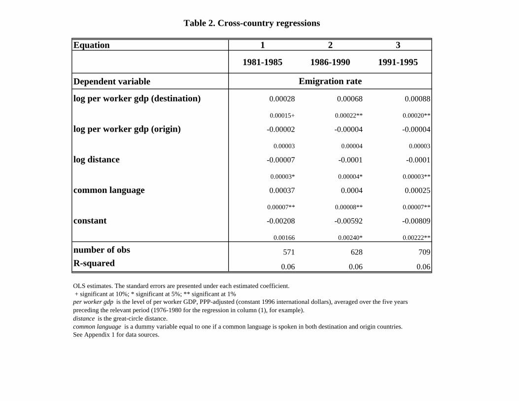
regressions (which are usually estimated in a cross section). In Table 2 I focus on a subsetof determinants and estimate their coefficients by exploiting only the cross-country variationin the data. I divide the period between 1981 and 1995 into three segments and I focus oneach at a time. I relate average emigration rates in each subperiod to the average incomeopportunities at home and abroad in the previous five-year interval (plus time-invariantvariables). In Table 3 I perform a similar exercise by estimating the model year by year.Due to the low number of observations in each regression, in Table 2 and Table 3 I don’t

36Interestingly, the coefficients of the two interaction variables are equal in absolute value.37Regression (6) does not include the regressors log distance, land border, common language and colony

since they are constant within country pairs and, therefore, they would be perfectly collinear with the dummyvariables.

17

control for country-specific fixed effects, which explains the difference in the magnitude of theeffects relative to the regressions in Table 1. The coefficients are still qualitatively consistentwith the panel-data results, though less precisely estimated.In Table 4 I run a few robustness checks of the panel-data results. In the first regression,

I use (within-country variation in) the terms of trade to instrument for (within-countryvariation in) the level of per worker GDP of both destination and origin countries. Termsof trade are correlated with the average real income of a country since they affect countries’purchasing power vis a vis goods produced by the rest of the world. In the first stage, theimpact of the terms of trade on per worker GDP is positive and significant at the 1% level, forboth destination and origin countries. In addition, if the assumption of small open economiesholds, terms of trade are unlikely to affect emigration rates directly or to be correlated withother country-level characteristics that have an impact on migration patterns (exclusionrestriction). Regression (1) shows that pull and push coefficients are robust to endogeneityissues as the instrumental variable estimates are consistent with my earlier results.In columns (2) and (3), I ask whether per worker GDP in the two locations is a good

measure of the mean income opportunities for migrant workers at home and abroad. I firstcontrol for the average schooling level in both countries in specification (2). Pull effects arestill estimated to be positive and significant (at the 1% level). In line with the theoreticalpredictions, the average skill level in the population of the destination (origin) country hasa negative (positive) impact on the emigration rate. In column (3) I control for per workerendowments of both skill and capital and again find that my prior findings are robust.In Table 5 I examine the predictions based on the extensions of the theoretical framework

of Section 2. I find only weak evidence of poverty constraints in regression (1) and confirm,in the following specification, my results on push and pull factors in terms of unemploymentrates. Third-country effects shape bilateral migration flows as expected, given that thecoefficient on the multilateral pull term is negative and significant.38 Finally, the size ofemigration rates is affected by the second moments of the income distributions in the twolocation in the way predicted by Borjas (1987) selection model.To conclude, I analyze network effects by introducing the lagged emigration rate(s) among

the explanatory variables (Table 6). Emigration rates clearly show a lot of inertia. How-ever, it’s unclear whether supply or demand factors explain the autocorrelation in bilateralmigration flows.39

38The multilateral pull term places migrants’ decision to move in a multi-country framework. It is inspiredby the multilateral trade resistance term in Anderson and van Wincoop (2003) (even though mine is anatheoretical measure).39Fixed-effects estimation of a dynamic model with a short panel (small T ) produces biased estimates.

This might explain the estimates in the first two columns of push and pull factors (which are different fromprevious ones). Once I use Arellano and Bond’s estimator, the coefficients become consistent with what Ipreviously found.

18

6 Conclusions

In this paper, I investigate economic and non-economic determinants of international migra-tion flows. This analysis both delivers estimates consistent with the predictions of a standardinternational-migration model and generates empirical puzzles.In particular, I find that pull factors, that is improvements in the income opportunities

in the destination country, significantly increase the size of emigration rates. This result,which appears to be very robust to changes in the specification of the empirical model, issurprising, given very restrictive immigration policies of the destination countries includedin the sample. The sign of the impact of push factors - that is, declining levels of per workerGDP in the origin country - is seldom consistent with the theoretical predictions of the modeland, when it is, the size of the effect is smaller than for pull factors and is almost alwaysinsignificant. Among the variables affecting the costs of migration, distance appears to beone of the most important ones. Its effect is negative, significant and quite steady acrossspecifications.The investigation of the determinants of international migration leads to other interesting

research questions. This analysis provides a framework to address policy-related issues, ashas been done in the trade gravity-model literature. The analysis of the impact of labourmovements on source and host economies - on their standards of living, for example - facesthe inherent problems of endogeneity of migration flows and reverse causality. Since thiswork helps isolate the exogenous determinants of immigrant flows, it is possible to use it toconstruct a first stage for this type of analyses (as in Frankel and Romer 1999, for example).By taking advantage of both the time-series and cross-country variation in an annual

panel data set, this paper makes progress in explaining the economic and non-economicdeterminants of international migration flows.

References

Adams, R. H. J. (1993). The economic and demographic determinants of internationalmigration in rural Egypt. Journal of Development Studies, 30(1):146—167.

Barro, R. and Lee, J. (2000). International data on educational attainment. Data Set.

Benhabib, J. (1996). On the political economy of immigration. European Economic Review,40:1737—1743.

Borjas, G. and Bratsberg, B. (1996). Who leaves? The outmigration of the foreign-born.Review of Economics and Statistics, 78(1):165—176.

Borjas, G. J. (1987). Self selection and the earnings of immigrants. American EconomicReview, 77:531—553.

19

Borjas, G. J. (1994). The economics of immigration. Journal of Economic Literature, pages1667—1717.

Borjas, G. J. (1995). The economic benefits from immigration. Journal of Economic Per-spectives, 9(2):3—22.

Borjas, G. J. (1999a). The economic analysis of immigration. In Ashenfelter, O. and Card,D., editors, Handbook of Labor Economics, chapter 28, pages 1697—1760. North-HollandElsevier Science, The Netherlands.

Borjas, G. J. (1999b). Heaven’s Door: Immigration Policy and the American Economy.Princeton University Press, Princeton, N.J.

Borjas, G. J. (2003). The labor demand curve is downward sloping: Reexamining the impactof immigration on the labor market. The Quarterly Journal of Economics, 40:1335—1374.Harvard University.

Chiswick, B. R. and Hatton, T. J. (2002). International migration and the integration oflabour markets. In Globalization in Historical Perspective. The University of ChicagoPress, Chicago, IL. Forthcoming.

Clark, X., Hatton, T. J., and Williamson, J. G. (2002). Where do U.S. immigrants comefrom, and why? National Bureau of Economic Research Working Paper No. 8998.

Coppel, J., Dumont, J.-C., and Visco, I. (2001). Trends in immigration and economicconsequences. OECD Economics Department Working Papers No. 284.

Davies, J. B. and Wooton, I. (1992). Income inequality and international migration. TheEconomic Journal, 102(413):789—802.

Davis, D. R. and Weinstein, D. E. (2002). Technological superiority and the losses frommigration. National Bureau of Economic Research Working Paper No. 8971.

Easterly, W., Kremer, M., Pritchett, L., and Summers, L. H. (1993). Good policy or goodluck? Country growth performance and temporary shocks. Journal of Monetary Eco-nomics, 32:459—483.

Easterly, W. and Sewadeh, M. (2002). Global development network growth database, Macrotime series. World Bank. Data Set.

Facchini, G. andWillmann, G. (2005). The political economy of international factor mobility.forthcoming Journal of International Economics.

20

Faini, R. (2002). Discussion of "International migration and the integration of labor markets"by B. Chiswick and T. Hatton. InGlobalization in Historical Perspective. The Universityof Chicago Press, Chicago, IL. Forthcoming.

Faini, R. and Venturini, A. (1994). Trade, aid and migrations. Some basic policy issues.European Economic Review, 37:435—442.

Frankel, J. A. and Romer, D. (1999). Does trade cause growth? The American EconomicReview, 89:379—399.

Freeman, G. (1992). Migration policy and politics in the receiving states. InternationalMigration Review, 26(4):1144—1167.

Freeman, G. (1995). Modes of immigration politics in liberal democratic states. InternationalMigration Review, 29(4):881—902.

Friedberg, R. and Hunt, J. (1995). The impact of immigrants on host country wages, em-ployment, and growth. Journal of Economic Perspectives, 9(2):23—44.

Goldin, C. (1994). The political economy of immigration restriction in the United States,1890 to 1921. In Goldin, C. and Libecap, G., editors, The Regulated Economy: AHistorical Approach to Political Economy, pages 223—257. University of Chicago Press,Chicago, IL.

Greenwood, M. J. (1997). Internal migration in developed countries. In Rosenzweig, M.and Stark, O., editors, Handbook of Population and Family Economics, Vol. 1B. North-Holland, Amsterdam.

Hatton, T. J. and Williamson, J. G. (2003a). Demographic and economic pressure on emi-gration out of Africa. Scandinavian Journal of Economics, 105:465—482.

Hatton, T. J. and Williamson, J. G. (2003b). What fundamentals drive world migration?revised version of National Bureau of Economic Research Working Paper No. 9159,forthcoming in G. Borjas and J. Crisp (eds), Poverty, international migration and asy-lum, Palgrave-Macmillan.

Helliwell, J. F. (1997). National borders, trade and migration. National Bureau of EconomicResearch Working Paper No. 6027.

Helliwell, J. F. (1998). How Much Do National Borders Matter?, chapter 5, pages 79—91.Brookings Institution Press.

Heston, A., Nuxoll, D. A., Summers, R., and Aten, B. (1995). Penn World Table version5.6a. Data Set.

21

Heston, A., Summers, R., and Aten, B. (2002). Penn World Table version 6.1. Center forInternational Comparisons at the University of Pennsylvania (CICUP). Data Set.

Hoddinott, J. (1994). A model of migration and remittances applied to Western Kenya.Oxford Economic Papers, 46:459—476.

ILO (1998). International labour migration database. International Labor Organization.

Jenks, R. (1992). Immigration and Nationality Policies of Leading Migration Nations. Centerfor Immigration Studies, Washington, DC.

Joppke, L. (1998). Why liberal states accept unwanted immigration. World Politics, 50:266—293.

Karemera, D., Oguledo, V. I., and Davis, B. (2000). A gravity model analysis of internationalmigration to North America. Applied Economics, 32(13):1745—1755.

Lucas, R. E. (2000). The effects of proximity and transportation on developing countrypopulation migrations. Boston University.

Mayda, A. M. (2003). Who is against immigration? A cross-country investigation of indi-vidual attitudes toward immigrants. Harvard University, dissertation chapter.

Mayda, A. M. and Patel, K. (2004). OECD countries migration policies changes. Appendixto International Migration: A Panel Data Analysis of Economic and Non-EconomicDeterminants, by Anna Maria Mayda. http://www.georgetown.edu/faculty/amm223/.

Money, J. (1997). No vacancy: The political geography of immigration control in advancedindustrial countries. International Organization, 51:685—720.

OECD (1997). International migration statistics for OECD countries. Data set.

OECD (2001). The employment of foreigners: Outlook and issues in OECD countries. InOECD Employment Outlook, chapter 5. OECD, Paris.

Pritchett, L. and Summers, L. H. (1996). Wealthier is healthier. The Journal of HumanResources, 31(4):841—868.

Ravenstein, E. (1885). The laws of migration. Proceedings of the Royal Statistical Society,XLVII(2):167—235.

Rodrik, D. (1995). Political economy of trade policy. In Grossman, G. and Rogoff, K., edi-tors, Handbook of International Economics, Vol.3, chapter 28, pages 1457—1494. North-Holland Elsevier Science, The Netherlands.

22

SOPEMI (1997). Trends in International Migration. Annual Report 1996. OECD, Paris.

SOPEMI (1999). Trends in International Migration. OECD, Paris.

SOPEMI (2000). Trends in International Migration. OECD, Paris.

Trefler, D. (1997). Immigrants and natives in general equilibrium trade models. NationalBureau of Economic Research Working Paper No. 6209.

Yang, D. (2003). Financing constraints, economic shocks, and international labor migra-tion: Understanding the departure and return of philippine overseas workers. HarvardUniversity, dissertation chapter.

Yang, P. Q. (1995). Post-1965 Immigration to the United States. Praeger, Westport, Con-necticut.

23

Equation 1 2 3 4 5 6

Dependent variable

log per worker gdp (destination) 0.00026 0.00026 0.00029 0.00028 0.00028 0.0002

0.00011* 0.00011* 0.00011* 0.00011* 0.00011* 0.00004**

log per worker gdp (origin) 0.00005 0.00005 0.00003 0.00004 0.00004 -0.00007

0.00009 0.00008 0.00008 0.00008 0.00008 0.00003*

log distance -0.0004 -0.00039 -0.00041 -0.00041 -0.00037

0.00009** 0.00009** 0.00009** 0.00009** 0.00008**

land border -0.00026 -0.00036 -0.00037 -0.00037

0.00019 0.00023 0.00023 0.00023

common language 0.00027 0.00022 0.00022 0.00019

0.00016+ 0.00016 0.00016 0.00012

colony -0.00001 0.00003 0.00003

0.00017 0.00017 0.00017

share of young population (origin) 0.00242 0.00222 0.00223 0.00129

0.00110* 0.00108* 0.00109* 0.00040**

per worker gdp (destination)*immig policy change 0.00006 0.00006 0

0.00002** 0.00002** 0.00001

per worker gdp (origin)*immig policy change -0.00006 -0.00006 0

0.00002** 0.00002** 0.00001

constant 0.00053 0.00044 -0.00027 -0.00008 -0.00045 -0.00168

0.00112 0.00107 0.00117 0.00115 0.0011 0.00050**

number of observations 8294 8294 8010 8010 8010 9767R-squared 0.24 0.25 0.25 0.25 0.25 0.85

per worker gdp is the level of per worker GDP, PPP-adjusted (constant 1996 international dollars), lagged by one year.distance is the great-circle distance. Land border equals one if the destination and origin countries share a land border.common language equals one if a common language is spoken in both destination and origin countries.colony is a dummy variable for pairs of countries ever in a colonial relationship.share of young population (origin) is the share of the population in the origin country aged 15-29.

See Appendix 1 for data sources.

Emigration rate

Table 1. Panel data regressions

OLS estimates. Destination and origin countries' dummy variables are included in each specification, except the last one (in regression 6, country-pairs dummy variables are included). Standard errors, clustered by country pairs, are presented under each estimated coefficient. + significant at 10%; * significant at 5%; ** significant at 1%

immigration policy change equals one if in that year the destination country's immigration policy became less restrictive, minus one if it became more restrictive, zero if there was no change in immigration policy.

2R 2R

Equation 1 2 3

1981-1985 1986-1990 1991-1995

Dependent variable

log per worker gdp (destination) 0.00028 0.00068 0.00088

0.00015+ 0.00022** 0.00020**

log per worker gdp (origin) -0.00002 -0.00004 -0.00004

0.00003 0.00004 0.00003

log distance -0.00007 -0.0001 -0.0001

0.00003* 0.00004* 0.00003**

common language 0.00037 0.0004 0.00025

0.00007** 0.00008** 0.00007**

constant -0.00208 -0.00592 -0.00809

0.00166 0.00240* 0.00222**

number of obs 571 628 709R-squared 0.06 0.06 0.06

OLS estimates. The standard errors are presented under each estimated coefficient. + significant at 10%; * significant at 5%; ** significant at 1%

distance is the great-circle distance.common language is a dummy variable equal to one if a common language is spoken in both destination and origin countries.See Appendix 1 for data sources.

Emigration rate

Table 2. Cross-country regressions

per worker gdp is the level of per worker GDP, PPP-adjusted (constant 1996 international dollars), averaged over the five years preceding the relevant period (1976-1980 for the regression in column (1), for example).

2R 2R

Equation 1 2 3 4 5 6 7 8

1981 1982 1983 1984 1985 1986 1987 1988

Dependent variable

log per worker gdp (destination) 0.0001 0.00079 0.00097 0.00038 0.00044 0.00052 0.00058 0.00062

0.00039 0.00034* 0.00033** 0.00018* 0.00017* 0.00021* 0.00024* 0.00023**

log per worker gdp (origin) -0.00008 -0.00006 -0.00004 -0.00002 -0.00002 -0.00003 -0.00003 -0.00003

0.0001 0.00008 0.00006 0.00003 0.00003 0.00004 0.00004 0.00004

log distance -0.00082 -0.00031 -0.00028 -0.00011 -0.00011 -0.00012 -0.00013 -0.00014

0.00018** 0.00011** 0.00008** 0.00003** 0.00003** 0.00004** 0.00005** 0.00004**

common language 0.00058 0.00033 0.00024 0.00032 0.00033 0.0004 0.00048 0.00043

0.00021** 0.00017+ 0.00013+ 0.00007** 0.00007** 0.00009** 0.00010** 0.00009**

share of young population (origin) 0.0056 0.00685 0.00476 0.00275 0.00265 0.00301 0.00342 0.00311

0.00321+ 0.00281* 0.00209* 0.00107* 0.00105* 0.00121* 0.00142* 0.00128*

constant 0.00532 -0.00682 -0.00855 -0.00359 -0.00419 -0.00494 -0.00561 -0.00599

0.00497 0.00385+ 0.00357* 0.00198+ 0.00193* 0.00233* 0.00272* 0.00254*

number of obs 165 220 275 551 551 551 551 551R-squared 0.19 0.11 0.11 0.07 0.07 0.08 0.08 0.08

OLS estimates. The standard errors are presented under each estimated coefficient. + significant at 10%; * significant at 5%; ** significant at 1%per worker gdp is the level of per worker GDP, PPP-adjusted (constant 1996 international dollars), lagged by one year.distance is the great-circle distance.common language is a dummy variable equal to one if a common language is spoken in both destination and origin countries.share of young population (origin) is the share of the population in the origin country aged 15-29.See Appendix 1 for data sources.

Emigration rate

Table 3. Yearly regressions

2R 2R

Equation 1 2 3 4 5 6 7

1989 1990 1991 1992 1993 1994 1995

Dependent variable

log per worker gdp (destination) 0.0011 0.00158 0.00171 0.0011 0.00128 0.0012 0.00093

0.00032** 0.00034** 0.00032** 0.00025** 0.00022** 0.00021** 0.00020**

log per worker gdp (origin) -0.00001 -0.00003 -0.00005 -0.00004 -0.00003 -0.00001 -0.00001

0.00005 0.00005 0.00005 0.00003 0.00003 0.00003 0.00003

log distance -0.00019 -0.00022 -0.00021 -0.00015 -0.00013 -0.00012 -0.00011

0.00005** 0.00006** 0.00005** 0.00003** 0.00003** 0.00003** 0.00003**

common language 0.00043 0.00029 0.00018 0.00019 0.00021 0.00019 0.00021

0.00011** 0.00011* 0.00010+ 0.00007** 0.00006** 0.00006** 0.00006**

share of young population (origin) 0.00443 0.00513 0.00405 0.00172 0.00175 0.00176 0.00156

0.00168** 0.00176** 0.00150** 0.00099+ 0.00090+ 0.00084* 0.00080+

constant -0.01102 -0.01602 -0.01706 -0.01047 -0.01266 -0.01213 -0.00918

0.00353** 0.00372** 0.00349** 0.00269** 0.00243** 0.00223** 0.00215**

number of obs 551 606 673 697 709 709 650R-squared 0.08 0.08 0.08 0.07 0.08 0.08 0.08

OLS estimates. The standard errors are presented under each estimated coefficient. + significant at 10%; * significant at 5%; ** significant at 1%per worker gdp is the level of per worker GDP, PPP-adjusted (constant 1996 international dollars), lagged by one year.distance is the great-circle distance.common language is a dummy variable equal to one if a common language is spoken in both destination and origin countries.share of young population (origin) is the share of the population in the origin country aged 15-29.See Appendix 1 for data sources.

Table 3. Yearly regressions (cont.)

Emigration rate

2R 2R

Equation 1 2 3 4

MethodInstrumental

Variables Estimation

OLS OLS TOBIT

Dependent variablelog per worker gdp (destination) 0.00041 0.00037 0.00053 0.00086

0.00015** 0.00011** 0.00019** 0.00036*

log per worker gdp (origin) -0.00023 0.00006 -0.00018 -0.00009

0.0002 0.0001 0.00013 0.00023

log distance -0.00031 -0.00037 -0.00029 -0.00143

0.00007** 0.00008** 0.00008** 0.00004**

common language 0.00007 0.0002 0.00015 0.0012

0.00008 0.00013 0.00011 0.00009**

share of young population (origin) 0.00065 0.00218 -0.00014 0.00683

0.001 0.00114+ 0.00113 0.00300*

log yrs schooling (destination) -0.00047 -0.00032

0.00015** 0.00018+

log yrs schooling (origin) 0.00008 0.00048

0.00012 0.00037

log capital per worker (destination) -0.00028

0.00013*

log capital per worker (origin) 0.00011

0.00014

constant -0.00001 -0.0009 0.00049 0.00063

0.00243 0.00126 0.00094 0.00407

number of obs 7411 7313 4103 8010

R-squared 0.23 0.25 0.26

In regression (1), I use terms of trade (lagged by one year) as an instrument for per worker GDP (lagged by one year) in both destination and origin country.per worker gdp is the level of per worker GDP, PPP-adjusted (constant 1996 international dollars), lagged by one year.distance is the great-circle distance. common language is a dummy variable equal to one if a common language is spoken in both destinationand origin countries. share of young population (origin) is the share of the population in the origin country aged 15-29.log yrs schooling is the log of the average schooling years in the total population over age 15, lagged by one year. log capital per worker is non-residential capital stock per worker (1985 intl. prices), lagged by one year.See Appendix 1 for data sources.

Emigration rate

Table 4. Panel data regressions: Robustness Checks

Destination and origin countries' dummy variables are included in each specification. Standard errors, clustered by country pairs, are presented under each estimated coefficient. + significant at 10%; * significant at 5%; ** significant at 1%

2R 2R

Equation 1 2 3 4

Dependent variable

log per worker gdp (destination) 0.00032 0.00038 0.00038

0.00012** 0.00013** 0.00018*

log per worker gdp (origin) 0.00083 0.00005 0.00007

0.00049+ 0.00008 0.00017

square of log per worker gdp (origin) -0.00004

0.00003

unemployment rate (destination) -0.00002

0.00001*

unemployment rate (origin) 0.00001

0.00001

multilateral pull -0.00006

0.00003*

origin country's relative inequality 0.00077

0.00039*

square of relative inequality -0.00028

0.00013*

log distance -0.00037 -0.00029 -0.00036

0.00008** 0.00008** 0.00007**

common language 0.00019 0.00028 0.00019

0.00012 0.00014* 0.00012

share of young population (origin) 0.00225 0.0007 0.0024

0.00111* 0.00083 0.00110*

constant -0.00433 0.00236 -0.0016 -0.00513

0.00272 0.00083** 0.00132 0.00182**

number of observations 8010 5148 8010 4028R-squared 0.24 0.19 0.24 0.18

See Appendix 1 for data sources.

Table 5. Panel data regressions: Economic determinants more in detail

Emigration rate

OLS estimates. Destination and origin countries' dummy variables are included in each specification. Standard errors, clustered by country pairs, are presented under each estimated coefficient. + significant at 10%; * significant at 5%; ** significant at 1%. See the end of Table 1 for definitions of the main variables used.

origin country's relative inequality gives a measure of the inequality in the origin country relative to the destination country (it equals the gini coefficient in the origin country divided by the gini coefficient in the destination country).

multilateral pull gives, for each destination/origin country pair, the average of (log per worker gdp (destination)-log distance) over all the other destination countries.

2R 2R

Equation 1 2 3

destination and origin countries d.v. country pair d.v. Arellano and Bond

estimator

Dependent variable

emigration rate(t-1) 0.91536 0.60247 0.66532

0.02641** 0.04166** 0.01485**

per worker gdp (destination) -0.00003 0.00005 0.00018

0.00003 0.00003+ 0.00007*

per worker gdp (origin) -0.00001 -0.00001 0.00003

0.00002 0.00003 0.00005

log distance -0.00003

0.00001**

constant 0.00066 -0.00041 0.00000

0.00027* 0.00025 0.00000

number of obs 8294 10101 6429R-squared 0.88 0.9

OLS estimates. The standard errors, clustered by country pair, are presented under each estimated coefficient.

Column (3): Arellano-Bond test that average autocovariance in residuals of order 1 is 0: H0: no autocorrelation z = -56.35 Pr > z = 0.0000.Column (3): Arellano-Bond test that average autocovariance in residuals of order 2 is 0: H0: no autocorrelation z = -0.48 Pr > z = 0.6329.

.

Emigration rate

Table 6: Dynamic regressions: network effects

+ significant at 10%; * significant at 5%; ** significant at 1%. per worker gdp is the level of per worker GDP, PPP-adjusted (constant 1996 international dollars), lagged by one year. distance is the great-circle distance. See Appendix 1 for data sources.In equation (3), I include the emigration rate lagged by one, two, three and four years (the coefficients on the latter three lags are not shown). The reason is that, only by introducing all these lags, I don't reject the null of zero autocovariance in residuals of order 2 (which is one of the requirements of the Arellano and Bond estimator).

2R 2R

Variable Obs Mean Std. Dev. Min Maxemigration rate 8010 0.0001324 0.0008154 0 0.0156894per worker gdp (destination) 8010 40681.73 5895.097 25251.65 55361.18per worker gdp (origin) 8010 20060.68 14106.18 1027.362 55361.18distance 8010 8.171532 0.8693557 5.08715 9.383615land border 8010 0.0268414 0.16163 0 1common language 8010 0.170412 0.3760178 0 1colony 8010 0.0384519 0.1922966 0 1years schooling (destination) 8010 9.713563 1.3133 6.837 11.865years schooling (origin) 7313 6.470704 2.521323 1.897 11.865capital per worker (destination) 6651 36168.39 12168.11 16992 76733capital per worker (origin) 4341 18267.41 13528.63 702 48135share of young population (origin) 8010 0.2612177 0.0302848 0.1951073 0.3152469unemployment rate (destination) 7667 6.730299 3.506799 0.5 14.1unemployment rate (origin) 5263 8.137606 5.269609 0.08 27.6origin country's relative inequality 1472 1.130724 0.3811316 0.3477012 2.59918

Data sources

Per worker GDP, PPP-adjusted (constant 1996 international dollars) is from the Penn World Tables, version 6.1.Distance, land border, common language, and colony (countries ever in a colonial relationship) are from Glick and Rose (2001).Years of schooling are from Barro and Lee (2000) data set.Capital per worker (Nonresidential Capital Stock per Worker, 1985 intl. prices) is from the Penn World Tables, version 5.6.The share of young population (origin) is based on data from the United Nations.The unemployment rate is from the World Development Indicators (2001), World Bank.

Data on terms of trade comes from the World Bank's Global Development Network Growth Database, Macro Time Series (2002).The data set on immigration policy changes was constructed by Anna Maria Mayda and Krishna Patel (2004) - see Appendix to the paper.All time-varying variables are lagged by one year.

Appendix 1. Summary Statistics (1980-1995) and Data Sources

The emigration rate (immigrant inflow from origin to destination country, divided by origin country's population) is from the IMS data set (OECD 1997).

The origin country's relative inequality is based on data on Gini coefficients from Deininger and Squire (1996) data set (only high-quality observations were used).

country of origin inflow country of origin inflow country of origin inflow country of origin inflowUK 17095 France 6072 Hong Kong 19334 Somalia 1264New Zealand 11045 Netherlands 6014 India 10437 UK 1068Vietnam 8048 USA 2930 Philippines 9441 Turkey 1042Hong Kong 5739 Germany 2916 UK 9034 Germany 805Philippines 5379 UK 2899 Vietnam 8791 Iraq 789Malaysia 3493 Morocco 2801 Poland 7550 Norway 699India 3069 Italy 2495 USA 7459 Sweden 612China 2934 Turkey 2239 China 6292 USA 606Former Yugoslavia 2790 Zaire 1966 Lebanon 3917 Iran 570South Africa 2441 Portugal 1435 Sri Lanka 3791 Vietnam 549Sri Lanka 2146 Japan 833 Portugal 3653 Former Yugoslavia 481Lebanon 2089 Spain 833 Jamaica 3543 Iceland 479USA 1724 Former Yugoslavia 829 Chinese Taipei 3255 Poland 448Fiji 1682 Greece 759 Guyana 3108 Thailand 366Poland 1608 Poland 655 El Salvador 2697 Pakistan 356Ireland 1462 China 589 Haiti 2243 Lebanon 335Chinese Taipei 1358 Algeria 382 Iran 2193 Netherlands 304Germany 1303 Tunisia 310 France 2070 France 269Former USSR 1021 total (above inflows) 36957 Former Yugoslavia 1933 Morocco 215Portugal 767 percentage change 13.46% South Korea 1584 Italy 200total (above inflows) 77193 Trinidad Tobago 1433 Finland 181percentage change -6.22% Romania 1241 total (above inflows) 11638

Pakistan 1037 percentage change 75.28%Former USSR 791Somalia 195total (above inflows) 117022percentage change 48.29%

total (above inflows) is the sum of the average immigrant inflows (1980-1995) by country of origin from the table.percentage change is the percentage change of the overall total during the period between 1980 and 1995.

Appendix 2. Average inflows into each destination country, by country of origin (1980-1995)

Australia (1983-1995) Belgium (1984-1995) Canada (1980-1995) Denmark (1990-1994)

country of origin inflow country of origin inflow country of origin inflow country of origin inflowMorocco 11892 Poland 117019 China 35425 Portugal 2170Algeria 9187 Former Yugoslavia 92124 USA 35367 France 1272Turkey 5777 Bosnia-Herzegovina 76836 Philippines 35121 Belgium 897Tunisia 3083 Turkey 68791 South Korea 21052 Germany 662Lebanon 2818 Romania 61910 Chinese Taipei 10882 Italy 441USA 2403 Italy 39184 UK 9614 Netherlands 281Haiti 2183 Croatia 24056 Brazil 6779 USA 256Portugal 2050 Former USSR 23365 Hong Kong 6296 Spain 124Vietnam 1761 Hungary 21835 Thailand 5913 total (above inflows) 6103Zaire 1437 Greece 20372 Germany 5334 percentage change 29.73%Poland 1422 Bulgaria 19245 Canada 3449Japan 1219 USA 17670 Peru 1008China 1084 Former CSFR 10692 total (above inflows) 176240Former Yugoslavia 1084 Portugal 9654 percentage change -42.10%Sri Lanka 899 Spain 4705Romania 891 Morocco 4375Cambodia 860 Slovenia 2658Spain 400 Tunisia 2249total (above inflows) 50450 total (above inflows) 616740percentage change -6.23% percentage change 24.85%

total (above inflows) is the sum of the average immigrant inflows (1980-1995) by country of origin from the table.percentage change is the percentage change of the overall total during the period between 1980 and 1995.* Figures for migrants from the former Yugoslavia to Germany do not include Croatia from 1992 and Bosnia-Herzegovina from 1993. Data from the former USSR to Germany does not include Russia from 1992.

Luxembourg (1983-1995)

Appendix 2. Average inflows into each destination country, by country of origin (1980-1995) (cont.)

France (1984-1995) Germany* (1984-1995) Japan (1980-1995)

country of origin inflow country of origin inflow country of origin inflow country of origin inflowTurkey 8363 Bosnia-Herzegovina 3728 Bosnia-Herzegovina 16972 Former Yugoslavia 18716Former Yugoslavia 7392 Denmark 2201 Iran 4048 Portugal 9085Morocco 6537 Sweden 1526 Finland 3880 Germany 8333Germany 5295 UK 1253 Norway 3118 Italy 8216UK 4575 USA 987 Former Yugoslavia 2840 France 4655Suriname 4416 Former Yugoslavia 868 Iraq 2051 Spain 4402USA 2303 Pakistan 682 Denmark 1877 Turkey 4195Belgium 2050 Iran 669 Somalia 1724 USA 2530France 1517 Vietnam 612 Chile 1631 UK 2407Poland 1148 Chile 537 Poland 1484 Austria 1728Italy 893 Somalia 468 Turkey 1214 Netherlands 1607total (above inflows) 44489 Sri Lanka 450 Ethiopia 947 Canada 687percentage change -16.04% Germany 399 Russian Federation 910 total (above inflows) 66561

total (above inflows) 14380 Lebanon 896 percentage change 24.68%percentage change 39.83% USA 831

Croatia 784Germany 761Romania 746UK 715Thailand 603India 369Greece 311total (above inflows) 48712percentage change 61.88%

total (above inflows) is the sum of the average immigrant inflows (1980-1995) by country of origin from the table.percentage change is the percentage change of the overall total during the period between 1980 and 1995.* Figures for migrants from the former Yugoslavia to Norway do not include Bosnia-Herzegovina from 1993.

Switzerland (1984-1995)Netherlands (1984-1995) Norway* (1984-1995) Sweden (1984-1995)

Appendix 2. Average inflows into each destination country, by country of origin (1980-1995) (cont.)

country of origin inflow country of origin inflowPakistan 5817 Mexico 199862India 5047 Philippines 51886Bangladesh 3796 Vietnam 45041USA 3776 China 32824Australia 2659 Dominican Republic 30471New Zealand 1964 India 29754Nigeria 1556 South Korea 29197Iran 1501 Former USSR 23231Japan 1474 El Salvador 21901Hong Kong 1287 Jamaica 20219Ghana 1093 Cuba 15174Canada 1035 Haiti 15168Sri Lanka 1021 UK 14939Philippines 986 Iran 14596South Africa 926 Poland 13534Turkey 822 Canada 12980Jamaica 775 Chinese Taipei 12962Malaysia 701 Colombia 12696Iraq 500 Laos 12165Kenya 481 Ireland 12054Poland 481 Guatemala 9328Thailand 444 Guyana 9243Germany 419 Cambodia 8108Cyprus 402 Pakistan 7725Morocco 380 Peru 7637Spain 363 Germany 7005Sweden 355 Hong Kong 6994France 345 Thailand 6270Italy 340 Ecuador 6189Netherlands 289 Nicaragua 5626Former Yugoslavia 276 Honduras 5507Portugal 223 Bangladesh 2684total (above inflows) 41534 total (above inflows) 702970percentage change -20.49% percentage change 35.79%

total (above inflows) is the sum of the average immigrant inflows (1980-1995) by country of origin from the table.percentage change is the percentage change of the overall total during the period between 1980 and 1995.

Appendix 2. Average inflows into each destination country, by country of origin (1980-1995) (cont.)

United Kingdom (1982-1995) United States (1980-1995)

1980 1981 1982 1983 1984 1985 1986 1987 1988 1989 1990 1991 1992 1993 1994 1995 TOTAL

disaggregateAustralia 69590 50729 57670 67543 83195 108277 113977 96460 98756 83289 57490 51623 64908 1E+06Belgium 9200 8000 8800 10000 9500 11100 15142 18924 41762 39228 39472 40214 251342Canada 100909 92308 85085 64669 64920 61187 71267 111124 116331 136398 162417 130550 141730 143184 132668 113164 2E+06Denmark 8922 10064 9614 8063 10744 47407France 25300 21000 22800 23300 25700 31600 60159 59608 50528 52160 37782 32275 442212Germany 108400 127700 159100 173600 223100 233600 485500 583500 925518 680315 475267 470590 5E+06Japan 266400 278100 103600 80900 100100 120100 122800 139300 191000 186600 176900 204500 214100 183245 186431 153948 3E+06Luxembourg 4350 3911 4537 5042 4832 6535 6502 7086 7182 6101 6679 6617 6649 76023Netherlands 23900 29000 33900 36300 37400 40800 48962 49868 50989 51268 35463 28738 466588Norway 8998 9707 10459 14962 15378 11190 9122 9465 10615 16154 11596 9480 137126Sweden 18300 19900 24800 27700 32900 44100 36100 25900 23100 43477 64099 26225 386601Switzerland 45500 46500 52800 57700 60400 64200 80994 85545 88695 81181 69362 65845 798722UK 43500 41540 40240 45020 38720 36980 39440 40170 42410 42310 41050 41950 42260 42650 578240US 418341 485642 490427 459946 443291 466307 495255 493507 528355 951871 1E+06 2E+06 805446 761217 675347 573784 1E+07Source: OECD (1997)

1980 1981 1982 1983 1984 1985 1986 1987 1988 1989 1990 1991 1992 1993 1994 1995 TOTALaggregate

Australia 93200 69800 78100 92400 113300 143500 145300 121200 121700 107400 76300 69800 87400 1E+06 76.06%Belgium 37200 37500 39300 40100 38200 43500 50500 54100 55000 53000 56000 53100 557500 45.08%Canada 143100 128600 121100 89200 88200 84300 99200 152100 161900 192000 214200 230800 252800 255800 223900 212200 3E+06 65.22%Denmark 15100 17500 16900 15400 15600 80500 58.89%France 51400 43400 38300 39000 44000 53200 102400 109900 116600 99200 69300 55700 822400 53.77%Germany 331100 398200 478300 473300 648500 770800 842400 920500 1E+06 986900 774000 788300 9E+06 53.90%Japan 362500 393100 134300 108100 131100 156500 157500 180300 234800 237400 223800 258400 267000 234500 237500 209900 4E+06 76.79%Luxembourg 6200 6000 6600 7400 7200 8200 8400 9300 10000 9800 9200 9200 9600 107100 70.98%Netherlands 37300 46200 52800 60900 58300 65400 81300 84300 83000 87600 68400 67000 792500 58.88%Norway 12800 15000 16800 23800 23200 18500 15700 16100 17200 22300 17900 16500 215800 63.54%Sweden 26100 27900 34000 37100 44500 58900 53200 43900 39500 54800 74800 36100 530800 72.83%Switzerland 58600 59400 66800 71500 76100 80400 101400 109800 112100 104000 91700 87900 1E+06 78.33%UK 53900 53500 51000 55400 47800 46000 49300 49600 53200 53900 52600 55600 55100 55500 732400 78.95%US 530600 596600 594100 559800 543900 570000 601700 601500 643000 1E+06 2E+06 2E+06 974000 904300 804400 720500 1E+07 84.47%Source: OECD (1997). % covered equals (TOTAL (disaggregate)/TOTAL (aggregate)) (in percentage terms).

Country of

Country of

% covered

Appendix 3. Total yearly inflows into each destination country, using data by country of origin (1980-1995)

Appendix 3. Total yearly inflows into each destination country, using total inflows data (1980-1995)

Figure 1: The actual emigration rate as a function of mean income opportunities in the destination and origin country and of mean moving costs

0

01

PI

Chh or 0 , =µ

0

01

PI S

0

01

PI D

),min(0

01

0

01

0

01

PI

PI

PI DS

=

0

01

PI D

0

01

PI

01µ

0

01

PI S

),min(0

01

0

01

0

01

PI

PI

PI DS

=

Figure 2: The impact of relative inequality on emigration rates according to Borjas (1987) selection model

Each curve represents the net labor income in Portugal and in the U.S. respectively. Income inequality is assumed to be higher in the U.S. than in the Portugal, consistent with the data. The Gini coefficient for Portugal was 36.76 in 1990, while in the U.S. it was 37.8 (Deininger and Squire 1996).

Each curve represents the net labor income in Brazil and in the U.S. respectively. Income inequality is assumed to be higher in Brazil than in the U.S., consistent with the data. The Gini coefficient for Brazil was 61.76 in 1985, while in the U.S. it was 37.26 ((Deininger and Squire 1996).

Brazil

0µCµµη −0

101

US

Portugal

0µ Cµµη −0101

US

6980

014

5300

3430

056

000

8430

025

5800

8900

1760

0

3830

014

4400

2732

0012

0760

0

1081

0039

3100

6000

1000

0

3640

087

600

1180

023

800

2230

074

800

5830

011

2100

4600

069

800

5306

0018

2720

0

80 82 84 86 88 90 92 94 96 80 82 84 86 88 90 92 94 96

80 82 84 86 88 90 92 94 96 80 82 84 86 88 90 92 94 96

Australia Belgium Canada Denmark

France Germany Japan Luxembourg

Netherlands Norway Sweden Switzerland

United Kingdom United States

tota

l im

mig

rant

infl

ow

yearGraphs by country of destination

Figure 3: Total immigrant inflow by destination country