International Journal of Heat and Mass Transfer 70 (2014) 864–874

Contents lists available at ScienceDirect

International Journal of Heat and Mass Transfer

journal homepage: www.elsevier .com/locate / i jhmt

A coupled lattice Boltzmann and finite volume method for naturalconvection simulation

0017-9310/$ - see front matter � 2013 Elsevier Ltd. All rights reserved.http://dx.doi.org/10.1016/j.ijheatmasstransfer.2013.11.077

⇑ Corresponding author. Tel.: +1 5738846936.E-mail address: zhangyu@missouri.edu (Y. Zhang).

Zheng Li a,b, Mo Yang b, Yuwen Zhang a,⇑a Department of Mechanical and Aerospace Engineering, University of Missouri, Columbia, MO 65211, USAb College of Energy and Power Engineering, University of Shanghai for Science and Technology, Shanghai 200093, China

a r t i c l e i n f o

Article history:Received 21 September 2013Received in revised form 26 November 2013Accepted 26 November 2013Available online 20 December 2013

Keywords:Nonequilibrium extrapolation schemeLattice Boltzmann methodFinite volume methodNatural convection

a b s t r a c t

A coupled lattice Boltzmann and finite volume method is proposed to solve natural convection in a dif-ferentially heated squared enclosure. The computational domain is divided into two subdomains and amessage passing zone is between them. The velocity and temperature fields are respectively solved usingD2Q9 and D2Q5 models in lattice Boltzmann method (LBM) while SIMPLE algorithm is applied to thefinite volume method (FVM). The velocity and temperature information transfers are fulfilled by a non-equilibrium extrapolation scheme. Pure FVM, pure LBM, and the coupled method with two different geo-metric settings are applied to solve the natural convection with different Rayleigh numbers. The resultsobtained from the coupled method agreed with those from pure FVM and LBM very well.

� 2013 Elsevier Ltd. All rights reserved.

1. Introduction

The fluid flow and heat transfer problems encountered in engi-neering applications span into different scales and there are differ-ent numerical methods for different scales. Molecular dynamics(MD) [1] can be applied to solve nano- and microscale problemswhile lattice Boltzmann method (LBM) is a typical mesoscopicscale method [2]. Finite volume method (FVM), on the other hand,is suitable for solving the macroscale problems [3]. The growingmultiscale problems must be solved with multiscale method sincethere is no method that is suitable for all the scales. There exist re-search works about the multiscale methods in the literature, e.g.,MD-LBM [4–6], MD-FVM [7–9] and LBM-FVM [10–12].

There are several models for the fluid flow and heat transferproblems in LBM. He et al. proposed the internal energy functionby relating internal energy with the kinetic energy of particle forthe incompressible fluid flow and heat transfer [13]. Then its simpli-fied thermal LBM model was advanced by Peng et al. [14] while Guoet al. introduced a coupled lattice BGK model based on Boussinesqassumption [15]. The D2Q9 and D2Q5 models were respectivelyused to solve the velocity and temperature fields [16]. Meanwhile,Semi-implicit Method for Pressure Linked Equation (SIMPLE) [17]is one of the most frequently used algorithms in FVM. The D2Q9and D2Q5 model were respectively used to solve the velocity andtemperature fields [16]. Meanwhile, Semi-Implicitly Method for

Pressure Linked Equation (SIMPLE) [17] is one of the most fre-quently used algorithms in FVM.

The objective of this paper is to combine the LBM and FVM as acoupled method to solve the fluid flow and heat transfer problem.The total computational domain is divided into FVM and LBMzones with a message passing zone between them. So there is anartificial boundary for each sub-domain. It is necessary to obtainthe artificial information from the other sub-domain to fulfill thecoupled method. For the fluid flow and heat transfer simulation,the problems under consideration are described using the macro-scopic variables, such as velocity, temperature, pressure and den-sity. And these variables in LBM are based on the density andenergy distributions results while they can be solved directly inFVM. Meanwhile macroscopic variables can be transferred fromthe density and energy distributions results directly. So it is quitestraightforward to obtain the FVM artificial boundary informationfrom the inner nodes in the LBM zone. But macroscopic variablesare not enough to obtain the corresponding density and energy dis-tributions results.

Latt [18] and Latt et al. [19] coupled LBM and finite differencemethod (FDM) for the pure fluid flow with the first-order expan-sion of the lattice Boltzmann equation. However, the FDM itselfhas the limitation when solving problems with complex computa-tional domain [3]. This shortfall restricts the development of LBM-FDM because the one of the most attractive advantages of LBM isits suitability to solve the problems in complex computationaldomain. Luan et al. [20] solved natural convection using theLBM-FVM with the general reconstruction operator [21]andobtained persuasive results. However general reconstruction

Nomenclature

c lattice speedcs speed of soundei particle speedF body forcefi density distributiong gravity acceleration (m/s2)G effective gravitational acceleration (m/s2)gi energy distributionH height of the cavity (m)Ma Mach numberNu Nusselt numberp pressure (N/m2)P nondimensional pressurePr Prandtl numberRa Rayleigh numbert time (s)T temperature (K)u horizontal velocity (m/s)

U nondimensional horizontal velocityv vertical velocity (m/s)V nondimensional vertical velocityV velocity

Greek Symbolsa thermal diffusivity (m2/s)b volume expansion coefficient of the fluid (K�1)h nondimensional temperaturel viscosity (N s/m2)m kinematic viscosity (m2/s)q density (kg/m3)s nondimensional timesv relaxation time for velocitysT relaxation time for energyxi value factor for velocityxT

i value factor for energy

Fig. 1. Nine directions in D2Q9 model.

Z. Li et al. / International Journal of Heat and Mass Transfer 70 (2014) 864–874 865

operator is newly proposed to fulfill the combine method whichmeans more validations are needed for the general reconstructionoperator itself. The nonequilibrium scheme [15] is a valid LBMboundary condition that was reported to have the second orderaccuracy. This scheme is applied to obtain the density and energydistributions on the LBM zone artificial boundary using the resultsin FVM zone in this paper. The LBM is solving a compressible prob-lem while FVM is based on incompressible assumption. Then apressure based correction method is applied to transfer densityfrom an incompressible domain to a compressible domain. Thennatural convections in a squared enclosure with different Rayleighnumbers are solved using the coupled method and the results arecompared with those obtained from pure LBM and pure FVM forvalidation of the coupled method.

2. Thermal LBM model

Two distribution functions are selected for the fluid flow andheat transfer in LBM. The density and energy distributions are rep-resented by fi and gi, which are related by the buoyancy force. Forthe velocity field, D2Q9 model is preferred. There are nine localparticle velocities on each computing node as shown in Fig. 1.These velocities are given by

ei ¼

ð0; 0Þ i ¼ 1c � cos ip

2 ;� sin ip2

� �i ¼ 2;3;4;5ffiffiffi

2p

c � cos ð2iþ1Þp4 ;� sin ð2iþ1Þp

4

� �i ¼ 6;7;8;9

8>><>>: ð1Þ

where c is the lattice speed.The density and momentum can be obtained by

q ¼X9

i¼1

fi ð2Þ

qV ¼X9

i¼1

eifi ð3Þ

By applying BGK model to Boltzmann equation [22], the equationfor density distribution, fi, is

fiðr þ eiDt; t þ DtÞ � fiðr; tÞ ¼1svðf eq

i ðr; tÞ � fiðr; tÞÞ þ Fi;

i ¼ 1;2; . . . 9 ð4Þ

where Dt is the time step, and feq is the equilibrium distributionfunction:

f eqi ¼ qxi 1þ ei � V

c2sþ ei � Vð Þ2

2c4s� V � V

2c2s

" #ð5Þ

where

xi ¼

49 i ¼ 119 i ¼ 2;3;4;51

36 i ¼ 6;7;8;9

8><>: ð6Þ

Then the Navier–Stokes equation can be obtained throughChapman-Enskog expansion [16] when the kinematic viscosity mis related to the relaxation time sv in Eq. (4) by:

m ¼ c2s sv �

12

� �Dt ð7Þ

where cs is the speed of sound that is related to the lattice speed by3c2

s ¼ c2

The buoyancy force can be obtained as:

Fi ¼ DtG � ðei � VÞp

f eqi ð8Þ

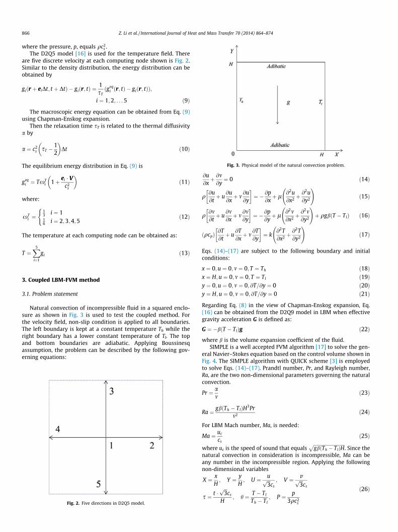
Fig. 3. Physical model of the natural convection problem.

866 Z. Li et al. / International Journal of Heat and Mass Transfer 70 (2014) 864–874

where the pressure, p, equals qc2s .

The D2Q5 model [16] is used for the temperature field. Thereare five discrete velocity at each computing node shown is Fig. 2.Similar to the density distribution, the energy distribution can beobtained by

giðr þ eiDt; t þ DtÞ � giðr; tÞ ¼1sTðgeq

i ðr; tÞ � giðr; tÞÞ;

i ¼ 1;2; . . . 5 ð9Þ

The macroscopic energy equation can be obtained from Eq. (9)using Chapman-Enskog expansion.

Then the relaxation time sT is related to the thermal diffusivitya by

a ¼ c2s sT �

12

� �Dt ð10Þ

The equilibrium energy distribution in Eq. (9) is

geqi ¼ TxT

i 1þ ei � Vc2

s

� �ð11Þ

where:

xTi ¼

13 i ¼ 116 i ¼ 2;3;4;5

(ð12Þ

The temperature at each computing node can be obtained as:

T ¼X5

i¼1

gi ð13Þ

3. Coupled LBM-FVM method

3.1. Problem statement

Natural convection of incompressible fluid in a squared enclo-sure as shown in Fig. 3 is used to test the coupled method. Forthe velocity field, non-slip condition is applied to all boundaries.The left boundary is kept at a constant temperature Th while theright boundary has a lower constant temperature of Tl. The topand bottom boundaries are adiabatic. Applying Boussinesqassumption, the problem can be described by the following gov-erning equations:

Fig. 2. Five directions in D2Q5 model.

@u@xþ @m@y¼ 0 ð14Þ

q@u@tþ u

@u@xþ m

@u@y

¼ � @p

@xþ l @2u

@x2 þ@2u@y2

!ð15Þ

q@m@tþ u

@m@xþ m

@m@y

¼ � @p

@yþ l @2m

@x2 þ@2m@y2

!þ qgbðT � TlÞ ð16Þ

ðqcpÞ@T@tþ u

@T@xþ m

@T@y

¼ k

@2T@x2 þ

@2T@y2

!ð17Þ

Eqs. (14)–(17) are subject to the following boundary and initialconditions:

x ¼ 0;u ¼ 0; m ¼ 0; T ¼ Th ð18Þx ¼ H; u ¼ 0; m ¼ 0; T ¼ Tl ð19Þy ¼ 0; u ¼ 0; m ¼ 0; @T=@y ¼ 0 ð20Þy ¼ H;u ¼ 0; m ¼ 0; @T=@y ¼ 0 ð21Þ

Regarding Eq. (8) in the view of Chapman-Enskog expansion, Eq.(16) can be obtained from the D2Q9 model in LBM when effectivegravity acceleration G is defined as:

G ¼ �bðT � TlÞg ð22Þ

where b is the volume expansion coefficient of the fluid.SIMPLE is a well accepted FVM algorithm [17] to solve the gen-

eral Navier–Stokes equation based on the control volume shown inFig. 4. The SIMPLE algorithm with QUICK scheme [3] is employedto solve Eqs. (14)–(17). Prandtl number, Pr, and Rayleigh number,Ra, are the two non-dimensional parameters governing the naturalconvection.

Pr ¼ am

ð23Þ

Ra ¼ gbðTh � TlÞH3Prm2 ð24Þ

For LBM Mach number, Ma, is needed:

Ma ¼ uc

csð25Þ

where uc is the speed of sound that equalsffiffiffiffiffiffiffiffiffiffiffiffiffiffiffiffiffiffiffiffiffiffiffiffiffiffiffiffigbðTh � TlÞH

p. Since the

natural convection in consideration is incompressible, Ma can beany number in the incompressible region. Applying the followingnon-dimensional variables

X ¼ xH; Y ¼ y

H; U ¼ uffiffiffi

3p

cs

; V ¼ vffiffiffi3p

cs

s ¼ t �ffiffiffi3p

cs

H; h ¼ T � Tl

Th � Tl; P ¼ p

3qc2s

ð26Þ

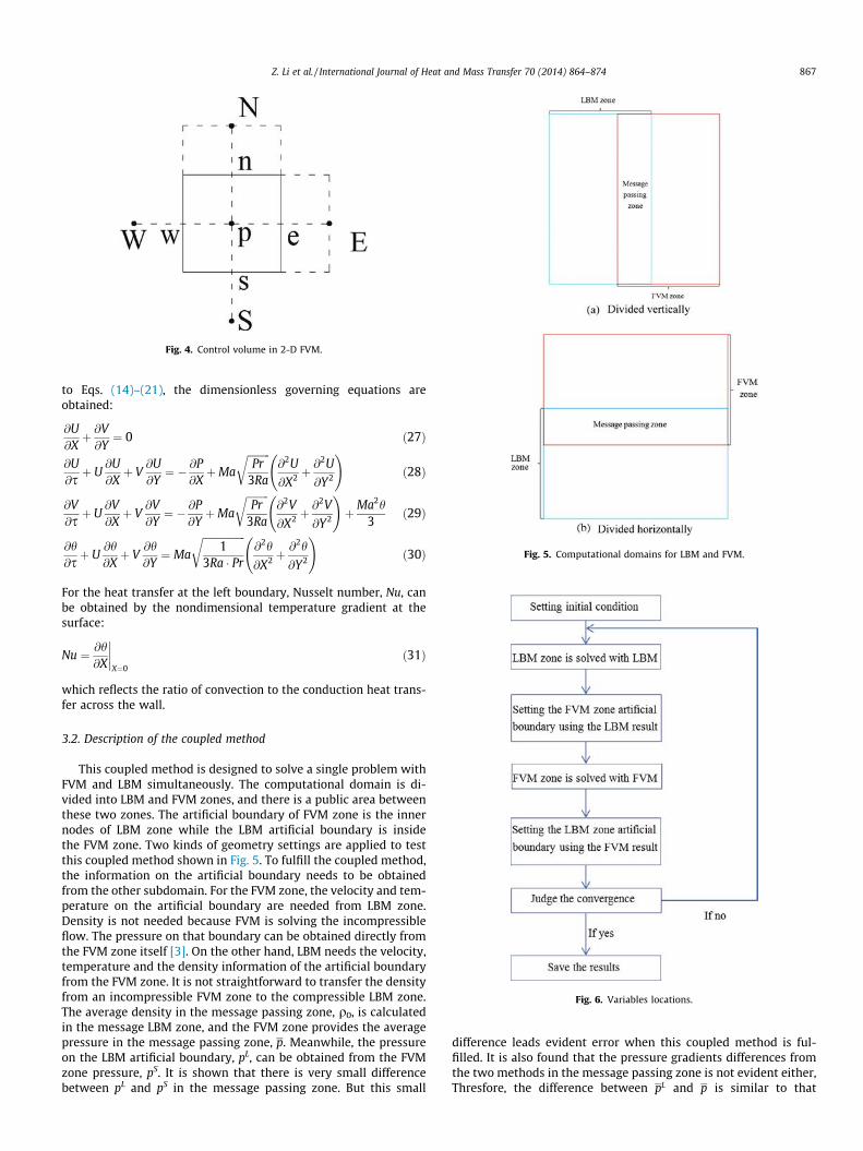
Fig. 4. Control volume in 2-D FVM.

Fig. 5. Computational domains for LBM and FVM.

Fig. 6. Variables locations.

Z. Li et al. / International Journal of Heat and Mass Transfer 70 (2014) 864–874 867

to Eqs. (14)–(21), the dimensionless governing equations areobtained:

@U@Xþ @V@Y¼ 0 ð27Þ

@U@sþ U

@U@Xþ V

@U@Y¼ � @P

@XþMa

ffiffiffiffiffiffiffiffiffiPr

3Ra

r@2U

@X2 þ@2U

@Y2

!ð28Þ

@V@s þ U

@V@Xþ V

@V@Y¼ � @P

@YþMa

ffiffiffiffiffiffiffiffiffiPr

3Ra

r@2V

@X2 þ@2V

@Y2

!þMa2h

3ð29Þ

@h@sþ U

@h@Xþ V

@h@Y¼ Ma

ffiffiffiffiffiffiffiffiffiffiffiffiffiffiffiffiffi1

3Ra � Pr

r@2h

@X2 þ@2h

@Y2

!ð30Þ

For the heat transfer at the left boundary, Nusselt number, Nu, canbe obtained by the nondimensional temperature gradient at thesurface:

Nu ¼ @h@X

����X¼0

ð31Þ

which reflects the ratio of convection to the conduction heat trans-fer across the wall.

3.2. Description of the coupled method

This coupled method is designed to solve a single problem withFVM and LBM simultaneously. The computational domain is di-vided into LBM and FVM zones, and there is a public area betweenthese two zones. The artificial boundary of FVM zone is the innernodes of LBM zone while the LBM artificial boundary is insidethe FVM zone. Two kinds of geometry settings are applied to testthis coupled method shown in Fig. 5. To fulfill the coupled method,the information on the artificial boundary needs to be obtainedfrom the other subdomain. For the FVM zone, the velocity and tem-perature on the artificial boundary are needed from LBM zone.Density is not needed because FVM is solving the incompressibleflow. The pressure on that boundary can be obtained directly fromthe FVM zone itself [3]. On the other hand, LBM needs the velocity,temperature and the density information of the artificial boundaryfrom the FVM zone. It is not straightforward to transfer the densityfrom an incompressible FVM zone to the compressible LBM zone.The average density in the message passing zone, q0, is calculatedin the message LBM zone, and the FVM zone provides the averagepressure in the message passing zone, p. Meanwhile, the pressureon the LBM artificial boundary, pL, can be obtained from the FVMzone pressure, pS. It is shown that there is very small differencebetween pL and pS in the message passing zone. But this small

difference leads evident error when this coupled method is ful-filled. It is also found that the pressure gradients differences fromthe two methods in the message passing zone is not evident either,Thresfore, the difference between pL and p is similar to that

Fig. 7. Flowchart.

868 Z. Li et al. / International Journal of Heat and Mass Transfer 70 (2014) 864–874

between pL and pS where pL is average pressure in the messagepassing zone calculated by the LBM zone results. Thus, it is reason-able to assume that [19]:

Fig. 8. Temperature fi

pL � pL ¼ pS � p ð32Þ

Regarding the relation between pressure and density in LBM, it canbe obtained that

qLc2s � q0c2

s ¼ pS � p ð33Þ

Then the unknown qL can be obtained that

qL ¼ q0pS � pq0c2

sþ 1

� �ð34Þ

The density information on the artificial boundary of LBM can beobtained by the result of the FVM result.

Staggered grid is applied to SIMPLE algorithm. Fig. 6 shows thelocations of variables in a control volume for LBM and FVM. Thevariables in LBM all locates on the corner of the control volumewhile velocity, pressure and temperature in FVM have differentlocations in the control volume. Central difference is applied tomessage passing processes due to the variable location differences.

After transferring the information from each other, the FVM andLBM zones need to be solved independently for each time step. Forthe FVM zone, temperatures and velocities on the four boundariesare known so that the solution procedure is straightforward. Thereare several choices for the LBM boundary conditions. Nonequilibri-um extrapolation scheme [15] is applied to both velocity and tem-perature fields in the solving process. Assuming xb is the boundarynode and xf is its nearby inner mode, the density and energy distri-bution at the artificial boundary are:

elds at Ra = 104.

Fig. 10. .Vertical velocity comparison on the centerline of cavity at Ra = 104.

Z. Li et al. / International Journal of Heat and Mass Transfer 70 (2014) 864–874 869

fiðxb; tÞ ¼ f eqi ðxb; tÞ þ fiðxf ; tÞ � f eq

i ðxf ; tÞ ð36Þ

giðxb; tÞ ¼ geqi ðxb; tÞ þ giðxf ; tÞ � geq

i ðxf ; tÞ ð37Þ

The temperatures on the boundaries are known in every time step,Eq. (37) can be applied to the thermal boundary conditions for Eq.(11). For the velocity field, the boundary density is only known onthe artificial boundary. It is common to approximate the densityon the fixed boundary by

qðxb; tÞ ¼ qðxf ; tÞ ð38Þ

Fig. 7 shows the flowchart of the computational procedure for thecoupled method.

4. Results and discussion

Natural convection in a squared enclosure is solved for threedifferent Rayleigh numbers at 104, 105 and 106 while the Prantlnumber is kept at 0.71. Pure LBM and pure FVM are reported inthe literature to be suitable for the natural convection in a cavity.Thus, these two methods are applied to solve the test cases. Ifthe LBM results agree with the FVM results, it can be concludedthat these results can be used as standard results for comparison.It can also verify that the codes for the two subdomains are reliable

(a) FVM

(c) Coupled method 1 Fig. 9. Streamline

in the coupled method. Then only the message passing method be-tween the two subdomains affects the results from the coupled

(b) LBM

(d) Coupled method 2s at Ra = 104.

870 Z. Li et al. / International Journal of Heat and Mass Transfer 70 (2014) 864–874

methods. Two coupled methods with different geometry settingsare applied. When the domain is divided vertically, it is referredto as Coupled Method 1. And the Coupled Method 2 divides thedomain horizontally as shown in Fig. 5. Temperature field,

Fig. 11. Nusselt numbers at Ra = 104.

(a) FVM

(c)Coupled method 1

Fig. 12. Temperature

streamline, vertical velocity on the centerline of cavity and Nusseltnumber on the left wall obtained from these four methods arecompared for the three cases. Nondimensional variables definedin Eq. (26) are applied in the comparisons.

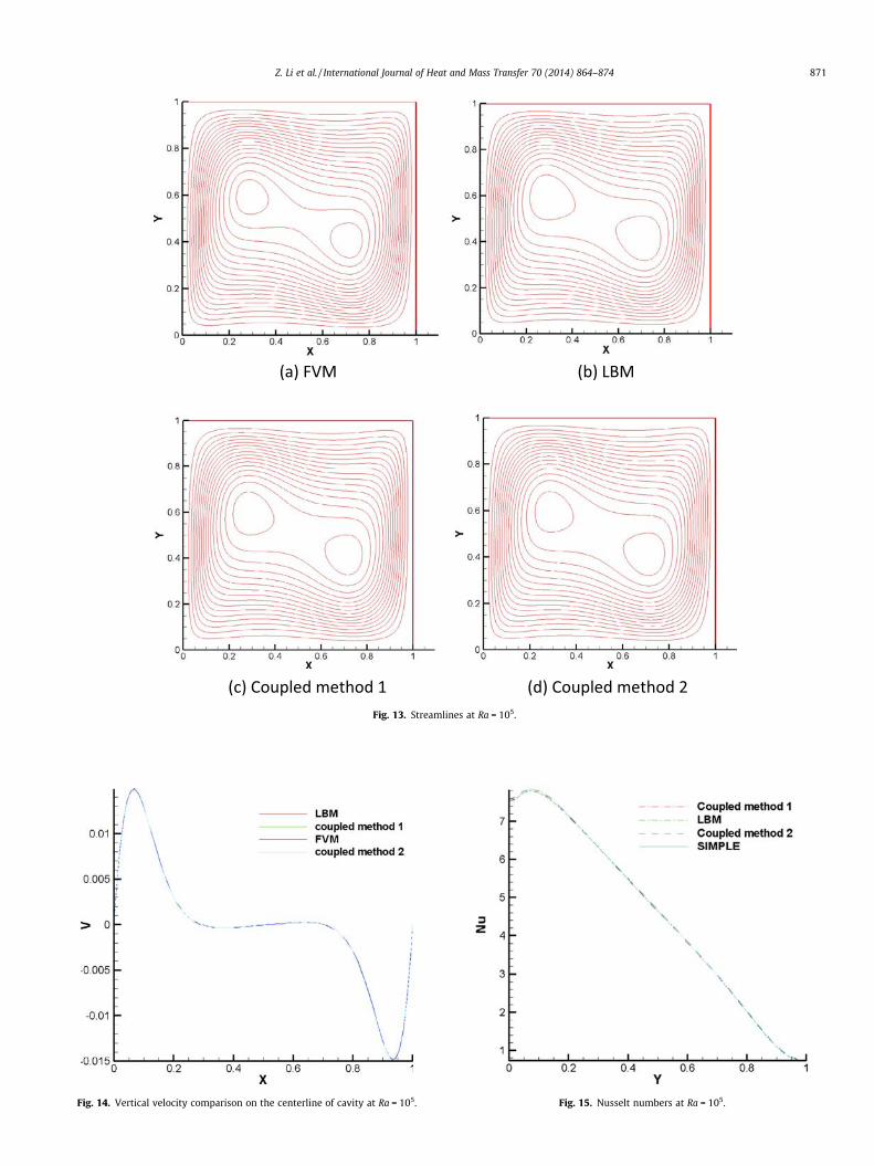
Figs. 8 and 9 show comparisons of temperature field andstreamlines obtained by different methods for the case that Ray-leigh number is 104. It is obvious that natural convection has dom-inated the heat transfer process and there is a stream line vertexnear the center of the cavity. Temperature fields and streamlinesobtained from pure LBM and pure FVM agree with each other wellas shown in Figs. 8 and 9. In addition, there is not any noticeabledifference between the results obtained from coupled methods 1and 2 and the results of coupled methods agreed with that fromthe pure FVM and pure LBM very well. Figs. 10 and 11 show thevertical velocity on the centerline of cavity and Nusselt numberat heated wall along the vertical direction of the enclosure ob-tained from different methods. There is a little difference betweenthe vertical velocity and Nusselt numbers obtained from pure LBMand pure FVM. The cause of this difference is that FVM is based onthe incompressible fluid assumption while LBM is based on com-pressible fluid assumption. Meanwhile the vertical velocity andNusselt number tendencies of the two coupled methods are veryclose to that of the two pure methods.

Figs. 12 and 13 show the temperature field and streamlinesobtained by different methods for the case that Rayleigh numberis 105. It can be see that the pure FVM and pure LBM reachsimilar temperature fields and streamlines. The convection effectbecomes more pronounced as the Rayleigh number increases.

(b) LBM

(d) Coupled method 2

fields at Ra = 105.

(a) FVM (b) LBM

(c) Coupled method 1 (d) Coupled method 2Fig. 13. Streamlines at Ra = 105.

Fig. 14. Vertical velocity comparison on the centerline of cavity at Ra = 105. Fig. 15. Nusselt numbers at Ra = 105.

Z. Li et al. / International Journal of Heat and Mass Transfer 70 (2014) 864–874 871

(a) FVM (b) LBM

(c) Coupled method 1 (d) Coupled method 2

Fig. 16. Temperature fields at Ra = 106.

872 Z. Li et al. / International Journal of Heat and Mass Transfer 70 (2014) 864–874

Two vertexes appear and the temperature gradients near the ver-tical boundary increase. The two coupled method results stillagree very well with that in the pure methods as shown inFigs. 12 and 13. For the centerline vertical velocity comparisonshown in the Fig. 14, it is very hard to find the difference betweeneach other. Coupled methods results agree with the pure methodsresults very well. Meanwhile, Fig. 15 shows that the differencebetween Nusselt numbers obtained from pure FVM and pureLBM is larger than that in Fig. 11; but the largest difference is stillround 2%. The Nusselt numbers from the two coupled methodsare closer to the results of pure LBM than that of the pure FVM.Since both coupled methods 1 and 2 have half regions withLBM that do not have incompressible fluid assumption, the fluidin the entire computational domain of the coupled methods canbe considered as compressible. The Nusselt number differencesbetween the two coupled methods are not larger than that be-tween the two pure methods.

Convection continues to become stronger when Rayleigh num-ber is increased to 106. Figs. 16 and 17 show that all four methodsyield the similar temperature fields and streamlines. There are stilltwo independent stream line vertexes that are closer to the verticalboundaries; this indicates a stronger convection effect comparingwith the results when Rayleigh number is 105. As for the centerlinevertical velocity and Nusselt number, Figs. 18 and 19 show that theresults from the coupled methods 1 and 2 are very close to thatfrom the pure LBM. And the differences between the two coupledmethods and pure FVM are still acceptable.

The results obtained by the coupled methods 1 and 2 are asgood as those from the pure FVM and pure LBM in all the threecases. The time consumption for the coupled method is higher thanthat of the pure FVM but lower than that of pure LBM. Comparingto FVM, LBM can show its advantage when solving the fluid flowand heat transfer problem in the complex geometry. ThereforeFVM is the most suitable method for the natural convection inthe cavity discussed above. Meanwhile the fluid flow and heattransfer problem in reality does not always have the regular geom-etry. For the cases that involve complex geometry as part of thecomputational; domain, the coupled methods discussed above willbe more suitable than both pure FVM and pure LBM.

5. Conclusion

A coupled LBM and FVM method is proposed for the fluid heattransfer problem. Nonequilibrium extrapolation scheme is used tocouple the macroscopic variables in FVM region to the mesoscopicvariables in LBM region. Two coupled methods with different geo-metric settings are employed to solve the natural convection in asquared enclosure and the results are compared with that obtainedfrom pure FVM and LBM. The results obtained from the four meth-ods agreed with each other very well at different Rayleigh numbersof 104, 105 and 106. The geometric settings do not affect the accu-racy of the coupled method. The results of this work demonstratedthat the coupled method is reliable to solve natural convectionproblems.

(a) FVM (b) LBM

(c) Coupled method 1 (d) Coupled method 2Fig. 17. Streamlines at Ra = 106.

Fig. 18. Vertical velocity comparison on the centerline of cavity at Ra = 106. Fig. 19. Nusselt numbers at Ra = 106.

Z. Li et al. / International Journal of Heat and Mass Transfer 70 (2014) 864–874 873

874 Z. Li et al. / International Journal of Heat and Mass Transfer 70 (2014) 864–874

Acknowledgment

Support for this work by the U.S. National Science Foundationunder grant number CBET-1066917 and Chinese National NaturalScience Foundation under Grants 51129602 and 51276118 isgratefully acknowledged.

References

[1] G. Grest, K. Kremer, Molecular dynamics simulation for polymers in thepresence of a heat bath, Phys. Rev. A 33 (1986) 3628–3631.

[2] S. Succi, Lattice Boltzmann Method for Fluid Dynamics and Beyond, OxfordUniversity Press, 2001.

[3] W.Q. Tao, Numerical Heat Transfer, Xi’an Jiaotong University Press, Xi’an, 2001.[4] T. Werder, J. Walther, P. Koumout, Hybrid atomistic-continuum method for the

simulation of dense fluid flows, J. Comput. Phys. 205 (1) (2005) 373–390.[5] A. Dupuis, E. Kotsalis, P. Koumoutsakos, Coupling lattice Boltzmann and

molecular dynamics models for dense fluids, Phys. Rev. E 75 (2007) 046704.[6] D. Fedosov, G. Karniadakis, Triple-decker, Interfacing atomistic–mesoscopic–

continuum flow regimes, J. Comput. Phys. 228 (4) (2009) 1157–1171.[7] S. O’Connell, P. Thompson, Molecular dynamics-continuum hybrid

computations: A tool for studying complex fluid flows, Phys. Rev. E 52(1995) R5792–R5795.

[8] E. Flekkoy, G. Wagner, J. Feder, Hybrid model for combined particle andcontinuum dynamics, Europhys. Lett. 52 (2000) 271–276.

[9] X. Nie, S. Chen, A continuum and molecular dynamics hybrid method formicro- and nano-fluid flow, J. Fluid Mech. 500 (2004) 55–64.

[10] B. Mondal, S. Mishra, Lattice Boltzmann method applied to the solution of theenergy equations of the transient conduction and radiation problems on non-uniform lattices, Int. J. Heat Mass Transfer 51 (2008) 68–82.

[11] B. Mondal, S. Mishra, The lattice Boltzmann method and the finite volumemethod applied to conduction–radiation problems with heat flux boundaryconditions, Int. J. Numer. Methods Eng. 78 (2) (2009) 172–195.

[12] H. Joshi, A. Agarwal, B. Puranik, C. Shu, A hybrid FVM–LBM method for singleand multi-fluid compressible flow problems, Int. J. Numer. Methods Fluids 62(2010) 403–427.

[13] X. He, S. Chen, G. Doolen, A novel thermal model for the lattice Boltzmannmethod in incompressible limit, J. Comput. Phys. 146 (1998) 282–300.

[14] Y. Peng, C. Shu, Y. Chew, Simplified thermal lattice Boltzmann model forincompressible thermal flows, Phys. Rev. E 68 (2003) 026701.

[15] Z. Guo, B. Shi, C. Zheng, A coupled lattice BGK model for the Boussinesqequations, Int. J. Numer. Methods Fluids 39 (2002) 325–342.

[16] C. Huber, A. Parmigiani, B. Chopard, M. Manga, O. Bachmann, LatticeBoltzmann model for melting with natural convection, Int. J. Heat Fluid Flow29 (2008) 1469–1480.

[17] S.V. Patankar, Numerical Heat Transfer and Fluid Flow, McGraw-Hill Book Co.,1980.

[18] J. Latt, Hydrodynamic Limit of Lattice Boltzmann Equations, Ph.D. Thesis,University of Geneva, 2007.

[19] J. Latt, B. Chopard, P. Albuquerque, Spatial coupling of a lattice Boltzmann fluidmodel with a finite difference Navier–Stokes solver, Technical Report, CornellUniversity, 2008.

[20] H. Luan, H. Xu, L. Chen, Coupling of finite volume method and thermal latticeBoltzmann method and its application to natural convection, Int. J. Numer.Methods Fluids 70 (2012) 200–221.

[21] H. Luan, H. Xu, L. Chen, Evaluation of the coupling scheme of FVM and LBM forfluid flows around complex geometries, Int. J. Heat Mass Transfer 54 (2011)1975–1985.

[22] S. Chen, G. Doolen, Lattice Boltzmann method for fluid flows, Annu. Rev. FluidMech. 30 (1998) 329–364.