international journal of engineering research and general...
TRANSCRIPT
International Journal of Engineering Research and General Science Volume 7, Issue 1, January-February, 2019 ISSN 2091-2730
16 www.ijergs.org
SIMULATION OF CONTROL CHANNELS FOR LTE NETWORKS
Vineesh.P, Thushara.T, Dechakka.M.P
Coorg Institute of Technology, Ponnampet, Coorg-District, Karnataka, [email protected]
Abstract-There has been evolution of mobile technologies from 3G to 4G in the past few years.System level simulations is crucial in
the evaluation of performance of new mobile technologies. . They aim at determining at what level predicted link level gains impact
the network performance. This paper presents a MATLAB computationally efficient LTE (Long Term Evaluation) control channel
simulator. LTE is a standard specified by the 3rd Generation Partnership Project.(3GPP).LTE offers improvement over UMTS and
HSPA. In LTE, physical layer conveys data and control information b/w eNodeB & UE (User Equipment).Simulator is used to
simulate the physical broadcast channel (PBCH) of LTE system. This physical channel carries information for UEs requiring to access
the network.
Keywords: 3G, 4G, LTE, Controlchannel, PBCH, enodeB, UE
INTRODUCTION
With the advent of Internet and wireless communication mobile data services are undergoing a tremendous growth. First generation
(1G) mobile phones had only voice facility. These were replaced by second generation (2G) digital phones with added fax, data and
messaging services. The third generation (3G) technology has added multimedia facilities to 2G phones.3G has paved way to 4G with
more advanced features.In order to evaluate the performance of new mobile technologies system level simulations are required. The
main objective of the paper is to simulate the physical broadcast channel (PBCH) for LTE (Long term evaluation networks) networks.
LTE SIMULATION
In the development and standardization of LTE, as well as the implementation process of equipment manufacturers, simulations are
necessary to test and optimize algorithms and procedures. This has to be performed on both, the physical layer (link-level) and in the
network (system-level) context. While link-level simulations allow for the investigation of issues such as Multiple-Input Multiple-
Output (MIMO) gains, Adaptive Modulation and Coding (AMC) feedback, modeling of channel encoding and decoding or physical
layer modeling for system-level, system-level simulations focus more on network-related issues such as scheduling, mobility handling
or interference management. The LTE system-level simulator supplements an already freely-available LTE link-level simulator. This
combination allows for detailed simulation of both the physical layer procedures to analyze link-level related issues and system-level
simulations where the physical layer is abstracted from link level results and network performance is investigated. The LTE system-
level simulator implementation offers a high degree of flexibility. For the implementation, extensive use of the Object-oriented
programming (OOP) capabilities of MATLAB, introduced with the 2010a Release has been made. Having a modular code with a clear
structure based in objects results in a much more organized, understandable and maintainable simulator structure in which new
functionalities and algorithms can be easily added and tested
OVERVIEW OF SIMULATOR
While link-level simulations are suitable for developing receiver structures, coding schemes or feedback strategies, it is not possible to
reflect the effects of issues such as cell planning, scheduling, or interference using this type of simulations. Simulating the totality of
the radio links between the User Equipments (UEs) and eNodeBs is an impractical way of performing system level simulations due to
the vast amount of computational power that would be required. Thus, in system-level simulations the physical layer is abstracted by
International Journal of Engineering Research and General Science Volume 7, Issue 1, January-February, 2019 ISSN 2091-2730
17 www.ijergs.org
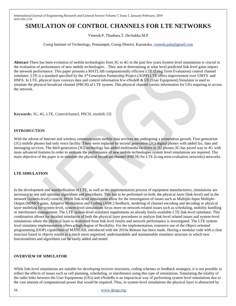
simplified models that capture its essential characteristics with high accuracy and simultaneously low complexity.Fig 1 depicts a
schematic block diagram of the LTE system-level simulator. Similar to other system-level simulators, the core part consists of a link
measurement model and a link performance model
Fig 1: Schematic block diagram of LTE Simulator
The link measurement model abstracts the measured link quality used for link adaptation and resource allocation. On the other hand
the link performance model determines the link Block Error Ratio (BLER) at reduced complexity’s figures of merit, the simulator
outputs traces containing throughput and error rates, from which their distributions can be computed. Implementation-wise, the
simulator flow follows the pseudo-code below. The simulation is performed by defining a Region Of Interest (ROI) in which the
enodeBs and UEs are positioned and a simulation length in Transmission Time Intervals (TTIs). It is only in this area where UE
movement and transmission of the Downlink Shared Channel (DLSCH) are simulated.
RUNNING A SIMULATION
The main file of the LTE Link Level Simulator is LTE_sim_main.m, though you may normally run the simulation through a batch file
such as LTE_sim_launcher.m, which performs the following tasks:
Loading a configuration file of choice
Executing the LTE_sim_main.m main simulation file.
SIMULATION RESULTS
BLER V/S SNR CURVES

International Journal of Engineering Research and General Science Volume 7, Issue 1, January-February, 2019 ISSN 2091-2730
18 www.ijergs.org
Block Error Rate (BLER) is used in LTE/4G technology to know the in-sync or out-of-sync indication during radio link monitoring
(RLM).BLER (in LTE) = No of erroneous blocks / Total no of Received Blocks. Normal in-sync condition is 2% of BLER and for
out-of-sync 10%.SNR refers to the signal to noise ratio.
The UE sends CQI feedback as an indication of the data rate which can be supported by the downlink channel. This helps the eNodeB
to select appropriate modulation scheme and code rate for downlink transmission. The UE determines CQI to be reported based on
measurements of the downlink reference signals. The UE determines CQI such that it corresponds to the highest Modulation and
Coding Scheme (MCS) allowing the UE to decode the transport block with error rate probability not exceeding 10%.The CQI report
not only indicates the downlink channel quality but also takes the capabilities of the UE’s receiver into account. A UE with receiver of
better quality can report better CQI for the same downlink channel quality and thus can receive downlink data with higher MCS. Table
1 shows modulation scheme, code rate along with efficiency for various CQI index
Table 1:CQI INDEX
Fig 2: Fig 2 shows the BLER v/s SNR plots for the 15LTE CQI indices

International Journal of Engineering Research and General Science Volume 7, Issue 1, January-February, 2019 ISSN 2091-2730
19 www.ijergs.org
SNR-CQI MAPPING PLOT
Before full commercial deployment of LTE, downlink SNR to CQI mapping for different multiple antenna techniques can be
of enormous significance for the operators. Such vital RF parameters should be tuned before full-fledged commercial launch.
In LTE, Adaptive Modulation and Coding (AMC) has to ensure a BLER value smaller than 10%. The SNR-to-CQI mapping
is required to achieve this goal. Fig 3 shows SNR-CQI mapping plot for 10% BLER.
Fig 3: SNR-CQI mapping plot
ANTENNA GAIN PLOT
Antenna gain is usually defined as the ratio of the power produced by the antenna from a far-field source on the antenna's
beam axis to the power produced by a hypothetical lossless isotropic antenna, which is equally sensitive to signals from all
directions. Usually this ratio is expressed in decibels, and these units are referred to as "decibels-isotropic" (dBi). An alternate
definition compares the antenna to the power received by a lossless half-wave dipole antenna, in which case the units are
written as dBd. Since a lossless dipole antenna has a gain of 2.15 dBi, the relation between these units is: gain in dBd = gain
in dBi - 2.15 dB . For a given frequency the antenna's effective area is proportional to the power gain. An antenna's effective
length is proportional to the square root of the antenna's gain for a particular frequency and radiation resistance. Due
to reciprocity, the gain of any antenna when receiving is equal to its gain when transmitting. Directive or directivity is a
different measure which does not take an antenna's electrical efficiency into account. This term is sometimes more relevant in
the case of a receiving antenna where one is concerned mainly with the ability of an antenna to receive signals from one
direction while rejecting interfering signals coming from a different direction.The antenna gain is always maximum when
θ=00.Fig 4 shows antenna gain versus the angular position in degrees.
Fig 4: Antenna gain plot

International Journal of Engineering Research and General Science Volume 7, Issue 1, January-February, 2019 ISSN 2091-2730
20 www.ijergs.org
MACROSCOPIC PATHLOSS V/S DISTANCE PLOT
The purposes of macroscopic modeling provide a means for predicting path loss for a particular application environment.
Fig 5 Macroscopic path loss v/s distance
Any individual path-loss model has a limited range of applicability and will provide only an approximate characterization for a
specific propagation environment. Fig 9.4 shows the plot for macroscopic path loss versus distance. Path loss increases with distance
as shown in Fig 5.
MACROSCOPIC PATHLOSS FOR DIFFERENT ENODEBS
Fig 6 shows the macroscopic path loss in dB for 3 eNodeBs in sector 1.The path loss is indicated in various colors on a scale starting
from 70 with different x and y positions
Fig 6: Macroscopic path loss for enodeBs in sector1
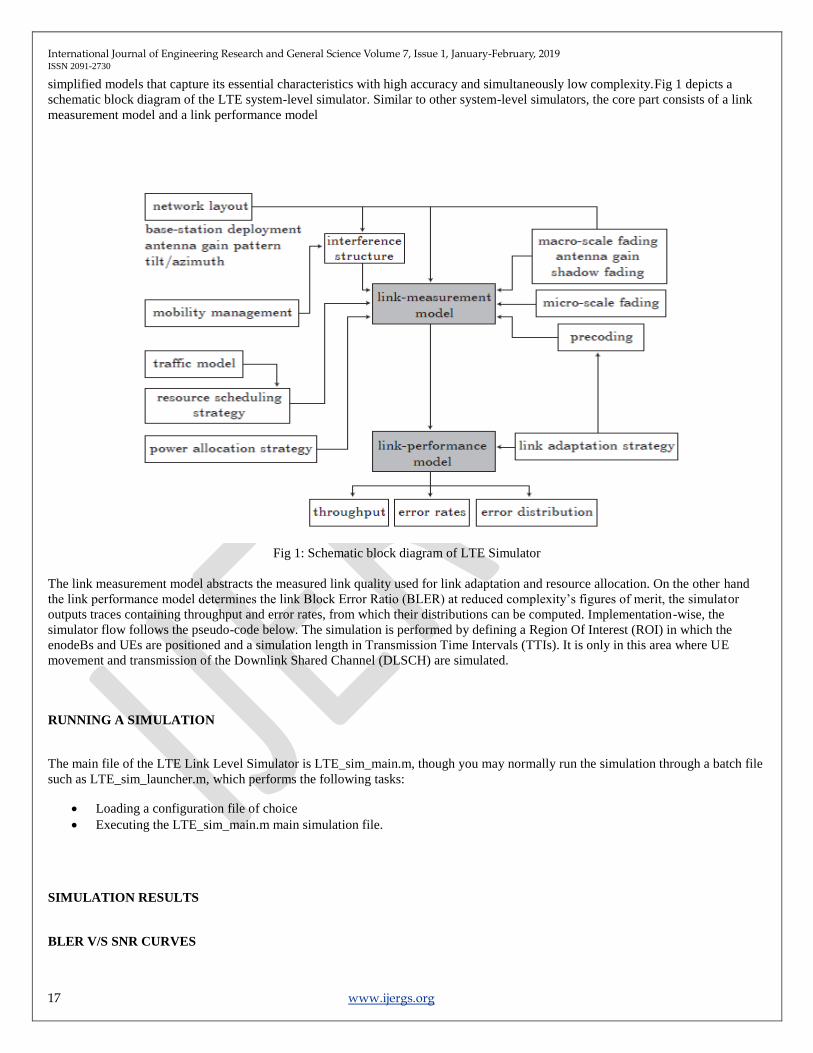
Fig 7 shows the macroscopic path loss in dB for 3 enodeBs in sector 2.The path loss is indicated in various colors on a scale starting
from 70 with different x and y positions
International Journal of Engineering Research and General Science Volume 7, Issue 1, January-February, 2019 ISSN 2091-2730
21 www.ijergs.org
Fig 7: Macroscopic path loss for enodeBs in sector2
Fig 8 shows the macroscopic path loss in dB for 3 enodeBs in sector 3.The path loss is indicated in various colors on a scale starting
from 70 with different x and y positions.
Fig 8: Macroscopic path loss for enodeBs in sector3
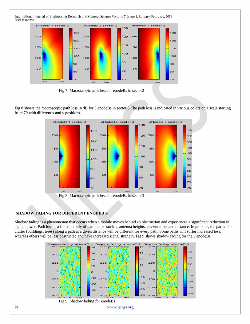
SHADOW FADING FOR DIFFERENT ENODEB’S
Shadow fading is a phenomenon that occurs when a mobile moves behind an obstruction and experiences a significant reduction in
signal power. Path loss is a function only of parameters such as antenna heights, environment and distance. In practice, the particular
clutter (buildings, trees) along a path at a given distance will be different for every path. Some paths will suffer increased loss;
whereas others will be less obstructed and have increased signal strength. Fig 9 shows shadow fading for the 3 enodeBs.
Fig 9: Shadow fading for enodeBs

International Journal of Engineering Research and General Science Volume 7, Issue 1, January-February, 2019 ISSN 2091-2730
22 www.ijergs.org
UE AND ENODEB POSITIONS
Fig 10 shows the UE positions with respect to eNodeBs.The 3 enodeBs are indicated in red color. The UE’s move from enodeB2 in
different directions. The handoff occurs between different UE’s and enodeBs as they move.
Fig 10: enodeBs and UE positions
UE INITIAL POSITION
Fig 11 shows the initial UE position, the 3 enodeBs in 3 sectors.
Fig 11: UE positions
MACROSCOPIC AND SHADOW FADING
The simulation is performed by defining a Region Of Interest (ROI) in which the enodeBs and UEs are positioned and a simulation
length in Transmission Time Intervals (TTIs). It is only in this area where UE movement and transmission of the Downlink Shared
Channel (DLSCH) are simulated. Sector SINR, calculated with distance dependent macro scale path loss and additional lognormal-
distributed space-correlated shadow fading is shown in Fig 12

International Journal of Engineering Research and General Science Volume 7, Issue 1, January-February, 2019 ISSN 2091-2730
23 www.ijergs.org
Fig `12: ROI max SINR (macroscopic and shadow fading)
Target sector CQIs calculated with distance dependent macro scale path loss and additional lognormal-distributed space-correlated
shadow fading is shown in Fig 13
Fig 13: Target sector CQI (macroscopic and shadow fading)
SINR difference calculated with distance dependent macro scale path loss and additional lognormal-distributed space-
correlated shadow fading is shown in Fig 14

International Journal of Engineering Research and General Science Volume 7, Issue 1, January-February, 2019 ISSN 2091-2730
24 www.ijergs.org
Fig 14: SINR difference (macroscopic and shadow fading)
The cell and sector assignment distance dependent macro scale path loss and additional lognormal-distributed space-
correlated shadow fading is shown in Fig 15
Fig 15: Cell and sector assignment (macroscopic and shadow fading)
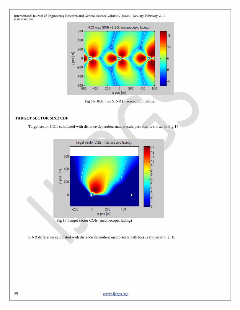
Sector SINR, calculated with distance dependent macro scale path loss is shown in Fig 16
International Journal of Engineering Research and General Science Volume 7, Issue 1, January-February, 2019 ISSN 2091-2730
25 www.ijergs.org
Fig 16 ROI max SINR (macroscopic fading)
TARGET SECTOR SINR CDF
Target sector CQIs calculated with distance dependent macro scale path loss is shown in Fig 17
Fig 17 Target sector CQIs (macroscopic fading)
SINR difference calculated with distance dependent macro scale path loss is shown in Fig 18

International Journal of Engineering Research and General Science Volume 7, Issue 1, January-February, 2019 ISSN 2091-2730
26 www.ijergs.org
Fig 18 SINR difference (macroscopic fading)
Cell and sector assignment calculated with distance dependent macro scale path loss is shown in Fig 19
Fig 19: Cell and sector assignment (macroscopic fading)
TARGET SECTOR SINR CDF
Fig 20 shows a plot of target sector SINR as a cumulative distributive function. The continuous line shows SINR CDF for
macro and shadow fading. The dotted lines show the SINR CDF of macro fading only.

International Journal of Engineering Research and General Science Volume 7, Issue 1, January-February, 2019 ISSN 2091-2730
27 www.ijergs.org
Fig 20: Target sector SINR CDF
CONCLUSION
The LTE Simulator has been used to simulate control channels of LTE network. The main purpose of this tool is to assess the network
performance. Testing Fractional Frequency Reuse (FFR) strategies implemented at the scheduler level, as well as the network impact
of different receiver types and channel quality feedback strategies, provided accurate modeling of those, can also be tested. These
simulations focus more on network-related issues such as scheduling mobility handling or interference management .The simulator
supplements a link level simulator. This combination allows for detailed simulation of both the physical layer procedures to analyze
link-level related issues and system-level simulations where the physical layer is abstracted from link level results and network
performance is investigated. The simulator for LTE networks need to be developed for investigating the interference behaviour of
femtocells placed within microcells. Thus it is necessary to simulate a multi-cell, multi-user and multi-carrier system in the downlink
for Single-Input, Single-Output (SISO) and Multiple-Input, Multiple-Output (MIMO) antenna configurations.
REFERENCES:
[1] Josep Colom Ikuno, Martin Wrulich, Markus Rupp “System level simulation of LTE networks”, Institute of Communications and
Radio-Frequency Engineering Vienna University of Technology, Austria Gusshausstrasse 25/389, A-1040 Vienna, Austria,May 2010
[2] C. Mehlf¨uhrer, M. Wrulich, J. C. Ikuno, D. Bosanska, and M. Rupp,“Simulating the long term evolution physical layer,” in Proc.
of the 17th European Signal Processing Conference (EUSIPCO 2009), Glasgow,Scotland, Aug. 2009.
[3] C. Shuping, L. Huibinu, Z. Dong, and K. Asimakis, “Generalized scheduler providing multimedia services over HSDPA,” in Proc.
IEEE International Conference on Multimedia and Expo, 2007, pp. 927–930.

International Journal of Engineering Research and General Science Volume 7, Issue 1, January-February, 2019 ISSN 2091-2730
28 www.ijergs.org
[4]E. Dahlman, S. Parkvall, J. Skold, and P. Beming, “3G Evolution: HSDPA and LTE for Mobile Broadband.” Academic Press, Jul.
2007.
[5] H. Claussen, “Efficient modelling of channel maps with correlated shadow fading in mobile radio systems,” Sept. 2005.
[6] J. Colom Ikuno, M. Wrulich, and M. Rupp, “Performance and modeling of LTE H-ARQ,” in Proc. ITG International Workshop on
Smart Antennas (WSA), Berlin, Germany, Feb. 2009.
[7] K. Brueninghaus, D. Astely, T. Salzer, S. Visuri, A. Alexiou, S. Karger, and G.-A. Seraji, “Link performance models for system
level simulations of broadband radio access systems,” Sept. 2005.
[8] M. ˇSimko, C. Mehlf¨uhrer, M. Wrulich, and M. Rupp, “Doubly Dispersive Channel Estimation with Scalable Complexity,” in
Proc. ITG International Workshop on Smart Antennas (WSA), Bremen, Germany, Feb. 2010.
[9] M. Castaneda, M. Ivrlac, J. Nossek, I. Viering, and A. Klein, “On downlink intercell interference in a cellular system,” in Proc.
IEEE 18th International Symposium on Personal, Indoor and Mobile Radio Communications (PIMRC), 2007, pp. 1–5.
[10] M. Wrulich, W. Weiler, and M.Rupp, “HSDPA performance in a mixed traffic network,” in Proc. IEEE Vehicular Technology
Conference (VTC) Spring 2008, May 2008, pp. 2056–2060.
[11] M. Wrulich, S. Eder, I. Viering, and M. Rupp, “Efficient link-to-system level model for MIMO HSDPA,” in Proc. of the 4th
IEEE BroadbandWireless Access Workshop, 2008.
[12] S. Schwarz, M. Wrulich, and M. Rupp, “Mutual information based calculation of the precoding matrix indicator for 3GPP
UMTS/LTE,” in Proc. ITG International Workshop on Smart Antennas (WSA), Bremen,Germany, Feb. 2010.
[13] Technical Specification Group RAN, “E-UTRA; LTE RF system scenarios,” 3rd Generation Partnership Project (3GPP), Tech.
Rep. TS 36.942, 2008-2009.
[14] W. C. Lee, Mobile Communications Engineering. McGraw-Hill Professional,1982.
[15] W. C. Jakes and D. C. Cox, Microwave Mobile Communications. Wiley-IEEE Press, 1994.
[16] X. Cai and G. Giannakis, “A two-dimensional channel simulation modelfor shadowing processes,” Vehicular Technology, IEEE
Transactions on,Nov. 2003.