1

International Fragmentation and Work Effort: Networks, Loyalty and Wages

Soonhee Park

University of Michigan

Abstract

This study examines how physical networks, loyalty and wages affect international fragmentation by a multinational firm and the work effect of its employees in a world composed of a developed country and a developing country. Fragmentation improves the firm’s ability to monitor. This increases employees’ effort. However, the headquarters cost for coordinating and monitoring the whole production process increases with the number of production stages. This cost limits the total stages. The international differences in networks, border barriers, loyalty and wages split the stages into the North and the South. (i) An increase in the Southern network increases outsourcing from North to South. The effort of the South relative to the North does not change. (ii) With globalization, Southern employees’ loyalty falls. Their effort relative to Northern employees’ effort falls. This decreases outsourcing. (iii) A rise in the Southern wage increases effort of the South relative to the North, and does not affect outsourcing. (iv) A rise in the Northern wage increases Northern effort relative to Southern effort. Its effect on outsourcing is ambiguous. This paper provides a new perspective on the motive of production fragmentation and firms’ organization decision by introducing the possibility of shirking and imperfect monitoring of employee effort.

Keywords: international fragmentation, work effort, shirking, networks, loyalty of employees, wages

JEL Classification: F12, F16

I am particularly grateful to Alan Deardorff for his guidance and insightful comments. I would like to thank John Laitner, Robert Stern and Katherine Terrell for valuable comments and suggestions. I also thank Eunyoung Hwang and Rahul Mukherjee for helpful discussions and comments. Department of Economics, University of Michigan, 611 Tappan Street, Ann Arbor, MI 48109, USA, Tel. (734) 665-6563, E-mail: soonheep@umich.edu

2

[1] Introduction

The world has seen a marked increase in global economic activities among countries. One of these trends

is international fragmentation – firms shift some part of production to a foreign country out of the home

country to produce the same product more efficiently. Factor endowment differences, factor intensity

differences and increasing returns to scale have been identified as the main reasons for the international

fragmentation of production.

Harris (2001) emphasizes increasing returns to scale of global trade networks – a set of links connecting a

large number of related demanders for and suppliers of intermediate inputs – that the firm runs, in order to

explain the phenomenon of international fragmentation among developed countries. The fixed cost of running

these networks is an important determinant of the extent of international fragmentation.1

The innovative development of physical network technology has given the world’s economies new

infrastructure for communications, such as the Internet and telecommunication networks. These have made

massive flows of information possible, and coordination of business partners scattered worldwide easier. Thus

the development of physical networks increases international trade. Freund and Weinhold (2002) find a

positive correlation between the Internet in a foreign country, and U.S. service imports and service exports.2

Also, the development of physical networks makes it possible to control from one location many business

divisions scattered geographically. This prompts the multinational firm’s activities. I study how physical

networks in a developed country (the North) and a developing country (the South) affect international

fragmentation of the vertical multinational firm.

Another strand of literature examines how work effort of workers influences factor prices, employment,

trade and welfare. 3 However, I explore how fragmentation of production affects work effort.4 In an

environment where ability of the headquarters to monitor employees is imperfect, employees would tend to

shirk, since they feel disutility in making an effort, and since there is the possibility that shirking is not

discovered by the headquarters. When the headquarters splits a single-stage production process into multiple-

stages, the split plays the role of dividing employees into smaller groups and assigns one group to each stage.

1 Deardorff (2001 a) explains that business and social networks reduce the costs of trade, and their welfare effect is likely to be beneficial for the world as a whole. 2 A 10% increase in internet use in a foreign country leads to about a 1.7% increase in the growth of U.S. service imports and a 1.1% increase in the growth of U.S. service exports from 1995 to 1997. 3 Copeland (1989) examines the effect of cross-country differences in the disutility of effort on the pattern of trade and welfare. Brecher (1992) analyzes the effect of a tariff on imports on employment and social welfare in an efficiency-wage model with explicit monitoring. Matusz (1996) shows that international trade leads to increased employment in both countries in a model in which intermediate inputs are produced under monopolistic competition and wages are determined according to efficiency wages of Shapiro-Stiglitz type (1984). Leamer (1999) examines the effects of factor intensity on effort level and wage at the sectoral level. 4 As another issue, Deardorff (2001 b) analyzes how fragmentation affects specialization and trade.

3

This makes it easier to detect the group of employees in which shirking arises. Employees raise their work

effort to avoid the penalty of a wage cut. Thus, fragmentation can lead to an increase in work effort in the

corresponding country. However, present studies associated with fragmentation seem to have overlooked this

characteristic of fragmentation.

As international economies become globalized and free trade zones resulting from an increase in free trade

agreements expand, the new competitive business environment makes employment relationships between

employees and firms unstable. Firms compete intensely with domestic and foreign firms for markets. The

volatility of their business increases and retaining employment becomes more difficult for the worker. Thus the

employment contracts of firms are easily broken, or the duration of employment shortens. Hence, loyalty of

employees to their firms falls.5 Since disutility of work effort of the employees with low loyalty is high, their

effort level decreases and thus their productivity becomes low. However, the new competitive environment

makes the employment relationship more unstable in the South compared to that in the North, since the South,

under a more protection that limits free trade, becomes relatively more exposed to international competition

than the North. This means loyalty in the South, and thus Southern work effort is relatively reduced. Therefore,

loyalty emerges as a factor affecting the determination of outsourcing to the South. I explore this relationship

between loyalty, work effort and international fragmentation.6

Wages in developing countries have fast increased. Can this increasing wage cause a Northern firm to

reduce outsourcing to the South? Since the increasing wage in the South increases production costs, the

Northern firm will tend to reduce outsourcing. However, since a higher wage gives Southern employees the

incentive to increase effort, the level of effort also rises. This reduces production costs in the South, which will

lead to the Northern firm increasing outsourcing. These opposite effects offset each other, so that the Southern

wage does not influence the degree of outsourcing. If the wage in developed countries rises, the effect on the

degree of outsourcing would depend on whether the wage effect on both the headquarters cost and the

production cost dominates the effort effect on the production cost.

Finally, when the Northern firm changes its mode of production from national fragmentation to

international fragmentation, I investigate how the number of total stages would change. I show that, compared

with national fragmentation, international fragmentation can increase, decrease or not change the number of

total stages according to differences in the amount of employment between the modes of production.

5 See Reichheld and Teal (1996), and Minkler (2004). 6 I will compare average employee tenures between the developed countries and the developing countries for inferring loyalty differences between the two.

4

As for the contribution of this paper to methodology, contrary to the existing method that focuses on

finding the level of output for an exogenously given number of stages, this paper focuses on how the firm

optimally splits a single-stage production process into multiple-stages, for exogenously given output. Also,

under international fragmentation, I explain how the firm optimally determines the number of total stages and

how the firm splits the stages between the North and the South.

[2] Model

[2-1] Autarkic Economy

This section examines how national fragmentation is determined in the North. National fragmentation is

defined as a production pattern locating all production stages within the national border, but all stages are

involved in producing a single final good.

Output increases more when the number of production stages increases though the technologies for

different stages do not have different factor intensities, so that a firm has an incentive to fragment its

production into many stages. This brings on specialization in production.

Increasing returns with respect to specialization can be represented by output increasing by more with an

increase in the variety of inputs (components). I develop a Leontief production function that has the

characteristic of increasing returns due to specialization.7 In products assembled from many components – for

example, electronics, automobiles and airplanes – each component is produced by technology specific to the

respective component, and all components are complementary to each other. If a component is removed, the

assembled product does not work. This description matches well with the property of the Leontief production

function.

There is a homogeneous final consumption good X which is supplied by a competitive industry. The

good X is produced by a production technology that consists of multiple production stages. The primary

production factor is labor. First, I consider the production function for good X .

,min{zx }b

el.

x is output of the good X . z is units of the intermediate good Z used. l is units of labor employed. b is

units of labor that are required to produce one unit of the good X . e is the level of work effort.

7 The increasing returns production functions of CES form (Ethier 1979) and Cobb-Douglas form (Edwards and Starr 1987) have been used in the literature. These functions have the feature that the inputs are substitutable for each other.

5

When the production process is split into multiple stages, each stage produces a distinct intermediate good,

using labor and an intermediate input produced at the previous stage. The final stage produces the finished

final good X . Let the production function for an intermediate good of the n th stage be of the Leontief form.

,min{ 1 nn zz })(

)(

nb

lne n , 2n ,…, n .

nz is output of an intermediate good nZ produced by the n th stage in the production with n stages for X .

1nz is units of an intermediate input provided by the )1( n th stage. nl is units of labor employed at the n th

stage.

The productivity of each stage depends on the degree of labor division; greater division of labor makes

labor more productive. If the degree of labor division is identical to the number of total stages, labor

productivity ))(

1(

nb rises with the number of total stages n . The reason is that if n increases, the units of

labor )(nb that each stage uses to produce one unit of the intermediate good become smaller. I define a

functional form for )(nb as follows:

)1

()(n

nb , where 1 , 0)(

n

nb. (1)

The condition 1 stands for the increasing returns due to labor division – specialization. It is well known

that the division of labor raises the productivity of the laborers working at each stage and leads to increasing

returns to specialization. However, for a given number of total stages n , the labor productivity in each stage is

the same, )(

1

nb.

The work effort is explained. I assume that the firm’s ability to monitor the employees who work in

production is imperfect. For better checking of the employees’ performance, the firm splits its production into

multiple-stage production. The split plays the role of dividing the employees into groups with a narrower range

of activities. This makes it easier to identify the group of employees in which shirking arises. If the number of

total stages increases, the firm can monitor the performance of the employees more effectively. This causes the

employees to work harder since they know that they will be penalized if idleness is detected. Thus their effort

is associated positively with the number of total stages n : 0)(

n

ne.

I now address how labor is employed by each stage when the firm has n stages. The first stage produces

its intermediate good 1Z with only labor. The production function of the first stage is

6

)(

)( 11 nb

lnez .

1z is output of the intermediate good produced at the first stage. 1l is labor employed by this stage. The

amount of labor of the first stage is )(

)( 11 ne

znbl . The labor employed per unit output of the intermediate good

1Z is )(

)(

ne

nb.

The second stage produces an intermediate good 2Z . This stage uses the intermediate good 1Z produced

in the first stage as an intermediate input and labor. Its production technology is

,min{ 12 zz })(

)( 2

nb

lne.

2z is output of 2Z . 1z is units of intermediate good 1Z used. Suppose that the second stage produces 2z

units of 2Z . Since the input-output coefficient on 1Z is 1, the second stage uses 1Z in the amount 2z . Thus

1z becomes 2z units: 21 zz . This means that the first stage will provide 2z units of 1Z . Then the

intermediate input used at the second stage embodies )(

)( 2

ne

znb units of labor since one unit of 1Z is produced

with )(

)(

ne

nb units of labor. The embodied labor

)(

)( 2

ne

znb becomes the labor demand of the first stage. The

second stage also employs labor, )(

)( 22 ne

znbl . Thus total labor embodied for the production of 2Z is the sum

of these two labor demands, )(

)(2

)(

)( 22

2

ne

znbl

ne

znb . The labor employed per unit of 2Z is

)(

)(2

ne

nb.

When this logic is generalized to the n th stage, the labor employed is explained as follows. The

production function of the n th stage is

,min{ 1 nn zz })(

)(

nb

lne n , 2n . (2)

7

If output of the n th stage is nz , this stage demands nz units of 1nZ as an intermediate input: nn zz 1 .

Since one unit of 1nZ at the )1( n th stage is produced with )(

)()1(

ne

nbn units of labor,8 nz units of 1nZ

embody )(

)()1(

ne

znbn n units of labor that are accumulated up to the )1( n th stage. Also the n th stage

employs labor, )(

)(

ne

znbl nn . Thus the total labor employed, which is accumulated until the n th stage, is

)(

)()1(

ne

znbn n)(

)(

ne

znnbl nn .

The production cost at the n th stage nPC is the product of the total labor employed and the wage.

)(

)(

ne

wznnbPC n

n , where nn . (3)

This cost is a cumulative cost from the first stage to the n th stage. As n becomes larger, nPC increases. As

the number of total stages n increases, nPC decreases since labor productivity rises with n (in other words,

)(nb is decreasing in n ). As nz becomes larger and w rises, production cost increases. If the work effort

)(ne rises, the cost falls since the labor input to produce one unit of good is reduced. Its production cost per

unit output of the good is

)(

)(

ne

wnnbpcn . (3’)

I call this the unit production cost.

The input-output coefficients on intermediate goods nZ , 1{n ,…, }n , are one, so that the demand

equals the supply for the respective intermediate goods. This makes the relationships among outputs of

intermediates nZ , 1n ,…, 1n , and final good X at n be

21 zz … nz ... nn zz 1 . (4)

The output at the final stage n equals the output of the final good X : xzn .

8 Since one unit of 1Z is produced with )(

)(

ne

nb units of labor, one unit of 2Z is produced with

)(

)(2

ne

nb units and 3Z

is produced with )(

)(3

ne

nb units, one unit of 1nZ should be produced with

)(

)()1(

ne

nbn units of labor.

8

However, the firm cannot expand endlessly the number of stages so as to increase the productivity of labor

employed. Difficulty in operating all the production stages would rise as the number of production stages

increases. Coordinating and monitoring the whole production process are necessary in order to lead to the

optimal performance of production. The role of the headquarters is to provide the services of coordination and

monitoring. The headquarters cost for providing these services rises as the number of production stages

increases. This would limit the number of stages.9 Also, I assume that the headquarters cost of providing the

services increases if the output of each stage nz increases. As a variable indexing the headquarters service, I

use total output which is increasing both in the number of stages and in the output level of each stage:

n

nnz

1

. (5)

The development of physical networks like the Internet and telecommunications network makes it easier

for a firm to access to networks, and to exchange information faster and in greater quantities. Traveling time

and cost of managers for coordination and monitoring decrease. Thus the network improves the efficiency of

the headquarters services. The home country and foreign country are both assumed to have networks, which

are considered public goods. The development of network technology has greatly reduced the cost of accessing

networks, so that the cost is very small relative to other costs. Thus every firm is assumed to use the networks

free.

To reflect the effect of the network on the headquarters cost, I need to define accessibility to the network.

N is the network size of the economy. This should be a large value such that 1N . At the n th stage, the

degree of accessibility to the network for each stage of the firm is assumed to be )(Nn . This has a value

between zero and one. The assumption of partial accessibility, 1)(0 Nn , implies that the individual firm

uses only a part of the network in the economy. If the economy has a larger network, the accessibility of each

stage to the network increases: 0)(

N

Nn. An increase in accessibility causes improvement in efficiency. I

assume that the stage n obtains improvement in efficiency by )(Nn times its output nz which is the index

of the headquarters services of the corresponding stage: nn zN )( . Then the total improvement in efficiency

9 Adam Smith (1937) explains that the division of labor (specialization) is limited by market size. Edwards and Starr (1987) explain that it is limited by indivisibilities of labor or setup costs in the transition of labor between production tasks. In Becker and Murphy (1992), specialization depends on the cost of coordinating specialized workers who perform complementary tasks, and on the extent of knowledge available.

9

for the firm with n stages is the sum of the improvement in efficiency of individual stages: n

n

nn zN )(

1

. For

simplicity, I assume that every stage has the same degree of accessibility )()( NNn for all 1{n ,…, }n .

Then the headquarters gets efficiency of

n

nn

n

nnn zNzN

11

)()( . (6)

I represent the degree of accessibility )(N as an index and specify the function constructing the index.

)1

1()(N

N , where 1N , 1)(0 N , 01)(

2

NN

N. (7)

When the effect of the network is considered, the index for actual headquarters services is the difference

between the headquarters services (5) and the improvement in efficiency (6):

n

nnzN

1

)}(1{ . This is re-

expressed, using N

N1

)}(1{ from (7),

n

nnz

N 1

1. (8)

The employees at the headquarters play the roles not only of coordinator but also of monitor. These jobs

are given many responsibilities for performance similar to those of the owner or principal. This makes

employees at headquarters become highly loyal to the firm and work honestly. Thus, I assume that these

employees do not shirk.10 This means that the headquarters employees provide effort maxe , which is the upper

bound of the set of possible effort levels that they can provide physically: ee max , for all e . Let be the

input requirement of effective labor – effective labor is defined as units of labor times an effort level per unit

of labor – per unit of headquarters service. Then, the number of units of labor included in is maxe

since

labor in the headquarters provides effort level maxe . Note that has a small value relative to the network size

of the economy N : N . The amount of labor employed for the headquarters is, from (8),

n

nnz

Ne 1max

, where N . (9)

10 In reality, the employees who work in the headquarters may shirk. However, I do not consider this case. The reason is that if they are shirkers, their role as monitor of the employees who work in production could be compromised.

10

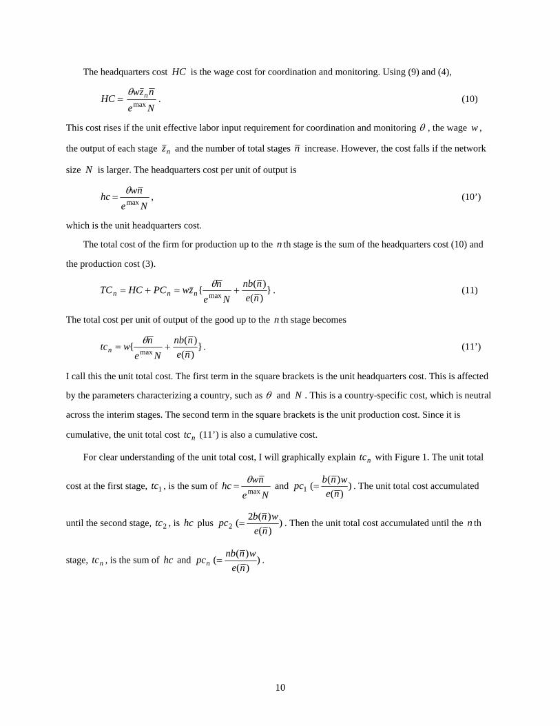
The headquarters cost HC is the wage cost for coordination and monitoring. Using (9) and (4),

HCNe

nzw nmax

. (10)

This cost rises if the unit effective labor input requirement for coordination and monitoring , the wage w ,

the output of each stage nz and the number of total stages n increase. However, the cost falls if the network

size N is larger. The headquarters cost per unit of output is

Ne

nwhc

max

, (10’)

which is the unit headquarters cost.

The total cost of the firm for production up to the n th stage is the sum of the headquarters cost (10) and

the production cost (3).

})(

)({

max ne

nnb

Ne

nzwPCHCTC nnn

. (11)

The total cost per unit of output of the good up to the n th stage becomes

})(

)({

max ne

nnb

Ne

nwtcn

. (11’)

I call this the unit total cost. The first term in the square brackets is the unit headquarters cost. This is affected

by the parameters characterizing a country, such as and N . This is a country-specific cost, which is neutral

across the interim stages. The second term in the square brackets is the unit production cost. Since it is

cumulative, the unit total cost ntc (11’) is also a cumulative cost.

For clear understanding of the unit total cost, I will graphically explain ntc with Figure 1. The unit total

cost at the first stage, 1tc , is the sum of Ne

nwhc

max

and 1pc )

)(

)((

ne

wnb . The unit total cost accumulated

until the second stage, 2tc , is hc plus 2pc ))(

)(2(

ne

wnb . Then the unit total cost accumulated until the n th

stage, ntc , is the sum of hc and npc ))(

)((

ne

wnnb .

11

Figure 1

I explain the costs of producing the final good. Recall that the output at the n th stage is x . Since the final

good X is produced at the final stage n of the production process, the total cost and the unit total cost of the

final stage are obtained by substituting n for n in nTC (11) and ntc (11’). Substituting )1

()(n

nb in (1),

nTC and ntc are

})(

{1

max ne

n

Ne

nxwTCn

, (12)

})(

{1

max ne

n

Ne

nwtcn

. (12’)

[2-1-1] Decision of Effort by Employee

An employee provides effort to the firm. The employee is compensated by a wage, which finances

consumption. Thus, she obtains higher utility, but feels disutility from effort. She determines a level of effort

where the difference between the utility and disutility is maximized. The employee has consumption c and her

utility is )(cu . She makes an effort e , max0 ee , and feels disutility )(ev . A low level of effort means that

the employee is very idle. 0e stands for complete idleness. If the employee provides full effort without

shirking, the level of effort is maxe and she becomes a fully effective worker.

The disutility of effort is also affected by the employee’s work ethic. Sennett (1998) and Minkler (2004)

contend that work ethic is influenced by the economic environment. With the development of the economy and

n

ntc

0

Unit costs

)(

)(

ne

wnnbpcn

n Stage number 1 2

2tc

1tc

ntc

nn pchctc

1pc2pc

npc

npc

Ne

nwhc

max

12

globalization, the firm faces a more competitive environment in domestic and international markets. The

volatility of its business increases, and its survival becomes more difficult. This situation makes for unstable

employment relations between the firm and its employees. Employment contracts with the firm are easily

broken, for example, the possibility of being unemployed rises, or the duration of employment shortens. This

causes the employees’ work ethic to be diminished: their loyalty to the firm weakens so that their motivation

and willingness to work hard are reduced (Reichheld and Teal 1996, and Minkler 2004).

In this paper, I do not deal with how the firm makes employment contracts to cope with the new

competitive business environment. Instead, I will focus on how the lower loyalty affects productivity and

production cost. Assume that employees with low loyalty have high disutility of effort. This assumption

implies that the disutility depends not only on effort but also on loyalty: );( ev . is the index for loyalty,

10 ; a high value of represents a high level of loyalty.

The firm expects its employees to work with maximal effort, maxe . It monitors their performance and

punishes the employees who are caught shirking. However, the headquarters’ ability to monitor is imperfect.

The employees would shirk on the job since effort involves disutility, and since there is a possibility that

shirking is not detected by the headquarters. Their performance would be lower compared with that in the

absence of shirking. Let P be the probability of an employee’s performance being checked by the

headquarters. If the performance of an employee is checked and if her level of effort is revealed to be below

the level of full effort such that max0 ee , she is penalized.11 Let ( P1 ) be the probability of an

employee’s performance not being checked. If the performance of an employee is not checked, the firm treats

the employee as a non-shirker, and thinks that she works with full effort maxe .12 Under this scheme, if the

detection probability is 0P , the employee provides no effort. The equilibrium level of effort is zero. If the

probability is 1P , her performance is perfectly revealed and thus she will provide full effort. The

equilibrium level of effort is maxe .

The employee can face two states. One is that she is not checked, with probability ( P1 ), and is

considered a non-shirker working with full effort maxe . She receives a wage w from the firm, which is

11 Copeland (1989), Brecher (1992), and Matusz (1996) based on the efficiency wage model assume that if shirking of the employee is caught, she is fired. However, I follow the assumption of Calvo and Wellisz (1978), that is, when the shirker is caught, she receives the penalty that her wage is cut. 12 Though the firm treats the employee as a non-shirker, it acknowledges that she can still shirk. However, without any evidence on her performance, if the firm regards her as a shirker, this incurs complaints from her and lowers her productivity. However, if the firm regards her as a non-shirker (i.e., a fully effective worker), this can (or cannot) increase her motivation to work hard. Anyway, the latter case of regarding a worker as the non-shirker can become beneficial to the firm than the former case of regarding the worker as the shirker.

13

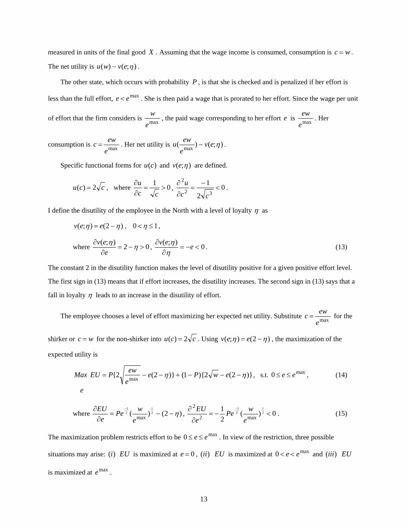
measured in units of the final good X . Assuming that the wage income is consumed, consumption is wc .

The net utility is );()( evwu .

The other state, which occurs with probability P , is that she is checked and is penalized if her effort is

less than the full effort, maxee . She is then paid a wage that is prorated to her effort. Since the wage per unit

of effort that the firm considers is maxe

w, the paid wage corresponding to her effort e is

maxe

ew. Her

consumption is maxe

ewc . Her net utility is );()(

maxev

e

ewu .

Specific functional forms for )(cu and );( ev are defined.

ccu 2)( , where 01

cc

u, 0

2

132

2

cc

u.

I define the disutility of the employee in the North with a level of loyalty as

)2();( eev , 10 ,

where 02);(

e

ev, 0

);(

eev

. (13)

The constant 2 in the disutility function makes the level of disutility positive for a given positive effort level.

The first sign in (13) means that if effort increases, the disutility increases. The second sign in (13) says that a

fall in loyalty leads to an increase in the disutility of effort.

The employee chooses a level of effort maximizing her expected net utility. Substitute maxe

ewc for the

shirker or wc for the non-shirker into ccu 2)( . Using )2();( eev , the maximization of the

expected utility is

Max )}2(2){1()}2(2{max

ewPee

ewPEU , s.t. max0 ee , (14)

e

where )2()( 21

21

max

e

wPe

e

EU, 0)(

2

121

23

max2

2

e

wPe

e

EU. (15)

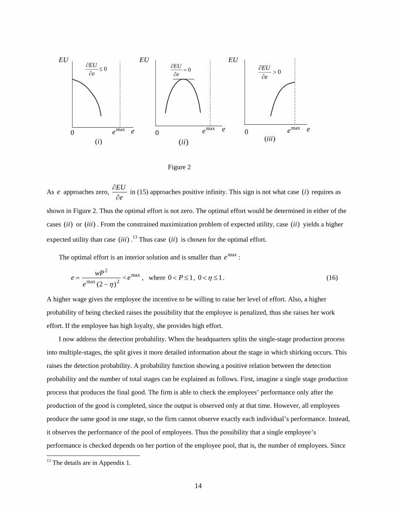
The maximization problem restricts effort to be max0 ee . In view of the restriction, three possible

situations may arise: )(i EU is maximized at 0e , )(ii EU is maximized at max0 ee and )(iii EU

is maximized at maxe .

14

Figure 2

As e approaches zero, e

EU

in (15) approaches positive infinity. This sign is not what case )(i requires as

shown in Figure 2. Thus the optimal effort is not zero. The optimal effort would be determined in either of the

cases )(ii or )(iii . From the constrained maximization problem of expected utility, case )(ii yields a higher

expected utility than case )(iii .13 Thus case )(ii is chosen for the optimal effort.

The optimal effort is an interior solution and is smaller than maxe :

e2max

2

)2( e

wP< maxe , where 10 P , 10 . (16)

A higher wage gives the employee the incentive to be willing to raise her level of effort. Also, a higher

probability of being checked raises the possibility that the employee is penalized, thus she raises her work

effort. If the employee has high loyalty, she provides high effort.

I now address the detection probability. When the headquarters splits the single-stage production process

into multiple-stages, the split gives it more detailed information about the stage in which shirking occurs. This

raises the detection probability. A probability function showing a positive relation between the detection

probability and the number of total stages can be explained as follows. First, imagine a single stage production

process that produces the final good. The firm is able to check the employees’ performance only after the

production of the good is completed, since the output is observed only at that time. However, all employees

produce the same good in one stage, so the firm cannot observe exactly each individual’s performance. Instead,

it observes the performance of the pool of employees. Thus the possibility that a single employee’s

performance is checked depends on her portion of the employee pool, that is, the number of employees. Since

13 The details are in Appendix 1.

EU

e

EU

e

EU

e 0 0 0maxe

0

e

EU 0

e

EU 0

e

EU

)(i )(ii

maxe maxe

)(iii

15

the firm competes in a perfectly competitive environment, its output is assumed to be exogenous.14 Thus the

number of employees, l , can be considered as given. This number is assumed to be large. The employees are

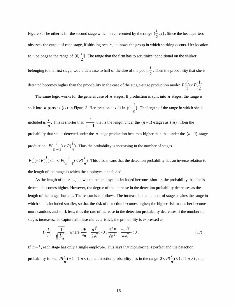
assumed to be distributed uniformly over the line in the range ,0( ]l as )(i in Figure 3. Then the size of the

employee pool is represented by this line.

Consider a single employee in the pool who is represented as one point, such as an arbitrary point, t , on

the line. The length of the range in which she is included is 1

l, where one in the denominator is the number of

total stages. This length of the range affects the probability that she is checked; I denote the probability simply

as a function of the length of the range: )1

(l

P .

Figure 3

If the firm changes the production mode from single-stage production to two-stage production, the

probability that she is checked would change. The first stage of the two-stage production produces a distinct

intermediate good that is assembled into the final good. The second stage produces the final good. The

employees engaged in production would be rearranged in two groups on the assumption that each employee is

assigned to only one stage. One group is for the first stage that is represented by the range ,0( ]2

l as )(ii in

14 In perfect competition, price equals average cost and marginal cost. Since the firm in my model has constant marginal cost, this equilibrium condition does not pin down a level of output. Also, this model is a partial equilibrium model that does not consider the factor market. Thus, the output level should be treated as given exogenously.

)(i One Stage:

)(ii Two Stages:

)(iv n Stages:

nl2 n

ln )1(

nl

2l

l 0

0

0

t

t

t

l

l

t 0 l

1)2(

nln

1nl

12nl

)(iii ( 1n ) Stages:

16

Figure 3. The other is for the second stage which is represented by the range ,2

(l

]l . Since the headquarters

observes the output of each stage, if shirking occurs, it knows the group in which shirking occurs. Her location

at t belongs to the range of ,0( ]2

l. The range that the firm has to scrutinize, conditional on the shirker

belonging to the first stage, would decrease to half of the size of the pool, 2

l. Then the probability that she is

detected becomes higher than the probability in the case of the single-stage production mode: )2

()1

(l

Pl

P .

The same logic works for the general case of n stages. If production is split into n stages, the range is

split into n parts as )(iv in Figure 3. Her location at t is in ,0( ]n

l. The length of the range in which she is

included is n

l. This is shorter than

1n

l that is the length under the )1( n -stages as )(iii . Then the

probability that she is detected under the n -stage production becomes higher than that under the )1( n -stage

production: )()1

(n

lP

n

lP

. Thus the probability is increasing in the number of stages.

)()1

(...)2

()1

(n

lP

n

lP

lP

lP

. This also means that the detection probability has an inverse relation to

the length of the range in which the employee is included.

As the length of the range in which the employee is included becomes shorter, the probability that she is

detected becomes higher. However, the degree of the increase in the detection probability decreases as the

length of the range shortens. The reason is as follows. The increase in the number of stages makes the range in

which she is included smaller, so that the risk of detection becomes higher; the higher risk makes her become

more cautious and shirk less; thus the rate of increase in the detection probability decreases if the number of

stages increases. To capture all these characteristics, the probability is expressed as

nln

lP

1)( , where 0

2

21

l

n

n

P, 0

4

23

2

2

l

n

n

P. (17)

If ln , each stage has only a single employee. This says that monitoring is perfect and the detection

probability is one, 1)( n

lP . If ln , the detection probability lies in the range 1)(0

n

lP . If ln , this

17

means that a single employee works in multiple stages. However, the firm is assumed to allocate more than

one of its employees to each of the stages, so that I exclude this case of ln .

Since a larger number of total stages increases the detection probability, the work effort of employees

increases with the number of total stages. Replacing n in (17) by n and substituting (17) for P in (16),

)(ne )()2( 2max l

n

e

w

, (18)

where 0)2(

)(2max

le

w

n

ne

, 0

)(2

2

n

ne. (19)

The first equation in (19) shows that the effort level increases if the number of total stages increases. And the

marginal increase in effort with respect to the number of total stages is constant. Thus the effort function (18)

is linear with respect to n . If 1n , 0)2( 2max

le

we

, where 10 . Also, since an employee cannot

provide more than maxe , (18) can determine the upper bound of the range of the number of total stages in

which effort is provided. This happens where the obtained effort becomes equalized to the maximum effort:

w

len

2max )}2({ . Figure 4 illustrates the above relation between the number of total stages and the effort

level in the range, w

len

2max )}2({1

.

Figure 4

)(ne

maxe

)(ne

w

le 2max )}2({

le

w2max )2(

n 1 0

18

[2-1-2] Equilibrium in National Fragmentation

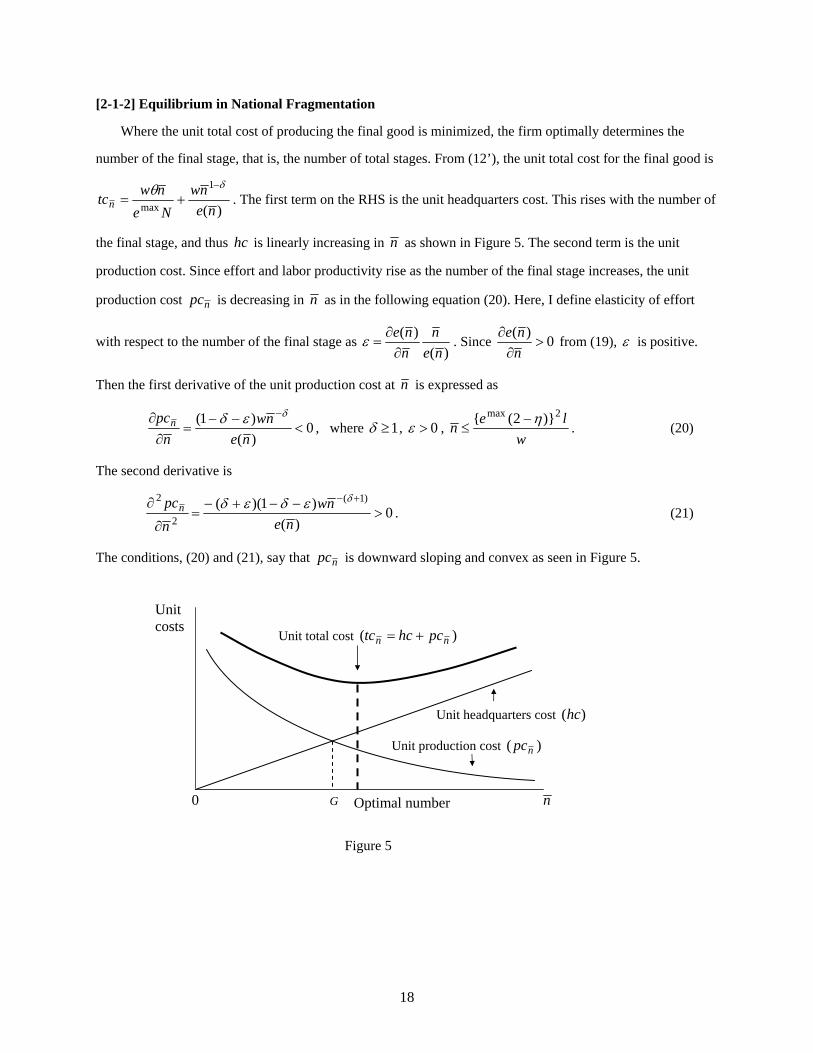
Where the unit total cost of producing the final good is minimized, the firm optimally determines the

number of the final stage, that is, the number of total stages. From (12’), the unit total cost for the final good is

)(

1

max ne

nw

Ne

nwtcn

. The first term on the RHS is the unit headquarters cost. This rises with the number of

the final stage, and thus hc is linearly increasing in n as shown in Figure 5. The second term is the unit

production cost. Since effort and labor productivity rise as the number of the final stage increases, the unit

production cost npc is decreasing in n as in the following equation (20). Here, I define elasticity of effort

with respect to the number of the final stage as )(

)(

ne

n

n

ne

. Since 0)(

n

ne from (19), is positive.

Then the first derivative of the unit production cost at n is expressed as

0)(

)1(

ne

nw

n

pcn

, where 1 , 0 , w

len

2max )}2({ . (20)

The second derivative is

0)(

)1)(( )1(

2

2

ne

nw

n

pcn

. (21)

The conditions, (20) and (21), say that npc is downward sloping and convex as seen in Figure 5.

Figure 5

Unit headquarters cost )(hc

Unit production cost )( npc

n 0

Unit total cost )( nn pchctc

Unit costs

Optimal number G

19

When hc and npc are summed, the graph of ntc is convex. The optimal number of stages is determined

where ntc is minimized with respect to n as shown in Figure 5.15 The first and second order conditions for

the cost minimization are

0})(

)1({

max

ne

n

New

n

tcn

, 02

2

2

2

n

pc

n

tc nn .

The cost-minimizing number of the final stage n is

1max

})(

)1({))((

ne

Nenen

. (22)

The number of stages is decreasing in )(ne and is convex: 0)(

))((

ne

nen and 0

)(

))((2

2

ne

nen. Note that the

number of stages is greater than one.16 The curve for ))(( nen is depicted in Figure 6. This means that if the

effort of employees increases, the necessity of dividing the production process would be reduced, and thus the

firm would decrease the number of total stages.

The equilibrium number of total stages n~

and the equilibrium effort e~ are determined by equations (18)

and (22). Substituting (18) for )(ne in (22),

1

12max

])}2(){1(

[~

w

lNen , (23)

12

1

1

1

1max }

)2({}

)1({)(~

l

wNee .

Also, n~

and e~ can be shown, by putting the graph for )(ne in Figure 4 and the curve for ))(( nen together in

the same space, as in Figure 6. n~

is smaller than the number of total stages where effort is maximal,

w

le 2max )}2({ . The employee provides e~ that is less than maxe .

15 The optimal number can also lie on the LHS of G, at the point G or on the RHS of G. The location depends on functional forms of the unit headquarters cost and the unit production cost. For convenience, the optimal number is located on the RHS of G in Figure 5. 16 The reasons are: 1 ; 1 from (18) since )(ne is proportional to n ; )(max nee ; and N in (9).

20

Figure 6

[2-2] Open Fragmented Economies

Revolutionary progress in communication technologies has weakened the link between specialization and

geographic concentration.17 Such progress makes communication across borders possible without physical

traveling and loss of time. Thus, regardless of production location, Northern firms can coordinate and monitor

all production stages remotely. This causes Northern firms to get the benefit of the low Southern wage, and

gives them incentives to relocate their production to the South.

I assume that the firm’s headquarters is located in the home country, the North. However, the headquarters

faces more difficulty running the Southern stages than the Northern stages. The first reason is Southern border

barriers, such as different culture, language and legal system. These require more headquarters services.

Second, since the network size of the South is assumed to be smaller than that of the North, the small Southern

network makes the Northern firm less efficient. Thus the firm faces a higher headquarters cost. However, the

low wage of the South reduces the firm’s production cost.

If the reduction in the production cost is larger than the increase in the headquarters cost, and thus if the

total cost with international fragmentation becomes lower than that with national fragmentation, the firm

would change the mode of production from national fragmentation to international fragmentation. The firm

will split the production stages across the two regions as a way of incurring the lowest total cost. I define

17 See Grossman and Rossi-Hansberg (2007 and 2009). They also say that a revolution in transportation makes it easy to transport partially processed goods quickly, and at lower cost. Thus specialization can be achieved without geographic concentration.

)(ne e~

n~

maxe

)(ne

w

le 2max )}2({

le

w2max )2(

))(( nen

))(( nen

0

1

21

international fragmentation as a production pattern locating some production stages in the North and some

production stages in the South, but all stages are involved in producing a single final good. The firm keeps the

headquarters in the North and might shift all production stages to the South. I exclude this case, but this is

explained in subsection [2-2-4].

To show that the total cost with international fragmentation is lower than that with national fragmentation,

we need to know the cost of the Northern firm as a multinational firm. For this, I first suppose ex-ante that

international fragmentation arises as follows: n̂ is the cutoff stage number at which the stages are split

between the North and the South; m is the number of total stages across both regions.

[2-2-1] Effort of Employee under International Fragmentation

The effort level of employees affects the multinational firm’s cost, therefore, I address how effort is

provided by employees under international fragmentation. The firm’s total employment in the North and the

South is fl . f denotes international fragmentation. The employees’ performance is monitored in each of the

m stages by the same headquarters regardless of which region they reside in. The size of any group in which

an individual employee is included is m

l f

. The detection probabilities for the Northern and Southern

employees are associated inversely with the size of group, and are the same.

The effort function of the Northern employees under international fragmentation has the same form as that

in (18) under national fragmentation, except that the detection probability is different. From (17), the detection

probability in the North changes from l

n to

fl

m.

)()2(

)(2max fl

m

e

wme

. (24)

Additionally, we need to know the disutility function of effort in order to pin down the effort level of the

employees in the South. Letting an asterisk denote the South, I define it as )2( *** ev , 10 * and

**

*

2

e

v. Using (24), the effort in the South is

)()2(

)(2*max*

**

fl

m

e

wme

. (25)

22

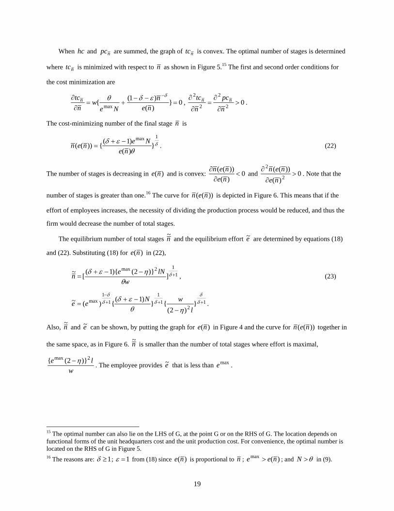
When the number of total stages m changes, Southern effort changes by the same proportion, m

1, as Northern

effort.18

I address the degrees of loyalty in the North and the South to compare the effort levels in both regions.

More global and more advanced economies (i.e., the North) have experienced more competition than less

global and less advanced economies (i.e., the South). The competitive environment in the North makes the

employment contracts between the firm and its employees more fragile, and thus duration of employment is

shortened. Under more protection that limits free trade, the South has been less exposed to international

competition, and has kept relatively stable employment relationships. To show these employment relations in

the North and the South, I compare average employment tenure of nine countries: Australia, Germany, the

Netherlands, the United Kingdom and the United States as the North, and Malaysia, the Philippines, the

Republic of Korea and Taiwan as the South.

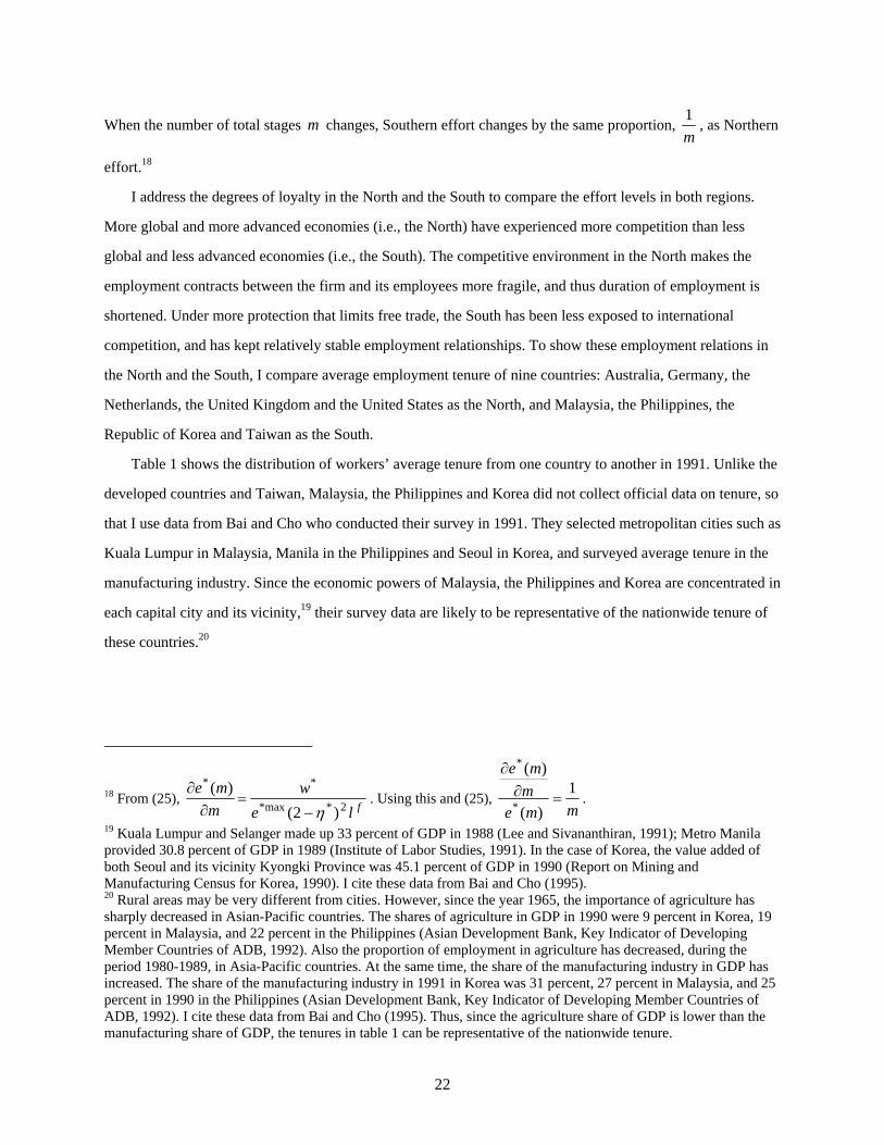
Table 1 shows the distribution of workers’ average tenure from one country to another in 1991. Unlike the

developed countries and Taiwan, Malaysia, the Philippines and Korea did not collect official data on tenure, so

that I use data from Bai and Cho who conducted their survey in 1991. They selected metropolitan cities such as

Kuala Lumpur in Malaysia, Manila in the Philippines and Seoul in Korea, and surveyed average tenure in the

manufacturing industry. Since the economic powers of Malaysia, the Philippines and Korea are concentrated in

each capital city and its vicinity,19 their survey data are likely to be representative of the nationwide tenure of

these countries.20

18 From (25), fle

w

m

me2**max

**

)2(

)(

. Using this and (25), mme

m

me1

)(

)(

*

*

.

19 Kuala Lumpur and Selanger made up 33 percent of GDP in 1988 (Lee and Sivananthiran, 1991); Metro Manila provided 30.8 percent of GDP in 1989 (Institute of Labor Studies, 1991). In the case of Korea, the value added of both Seoul and its vicinity Kyongki Province was 45.1 percent of GDP in 1990 (Report on Mining and Manufacturing Census for Korea, 1990). I cite these data from Bai and Cho (1995). 20 Rural areas may be very different from cities. However, since the year 1965, the importance of agriculture has sharply decreased in Asian-Pacific countries. The shares of agriculture in GDP in 1990 were 9 percent in Korea, 19 percent in Malaysia, and 22 percent in the Philippines (Asian Development Bank, Key Indicator of Developing Member Countries of ADB, 1992). Also the proportion of employment in agriculture has decreased, during the period 1980-1989, in Asia-Pacific countries. At the same time, the share of the manufacturing industry in GDP has increased. The share of the manufacturing industry in 1991 in Korea was 31 percent, 27 percent in Malaysia, and 25 percent in 1990 in the Philippines (Asian Development Bank, Key Indicator of Developing Member Countries of ADB, 1992). I cite these data from Bai and Cho (1995). Thus, since the agriculture share of GDP is lower than the manufacturing share of GDP, the tenures in table 1 can be representative of the nationwide tenure.

23

Table 1 Distribution of Employment by Enterprise Tenure, 1991

(a) Data were collected in 1990. (b) In Kuala Lumpur, Malaysia, 739 men and 706 women were surveyed from May to August, 1991. (c) In Manila, the Philippines, 784 men and 786 women were surveyed from May to August 1991. (d) In Seoul, Korea, 701 men and 689 women were surveyed in the first survey took place in February and March,

1991, and in the second survey took place in August 1991. (e) Data for men are not available. Data for women are not available. Source: OECD Employment Outlook (1993) for developed countries, Bai and Cho’s survey report (1995) for Malaysia, the Philippines and Korea, and Report on the Manpower Utilization Survey (2005) for Taiwan

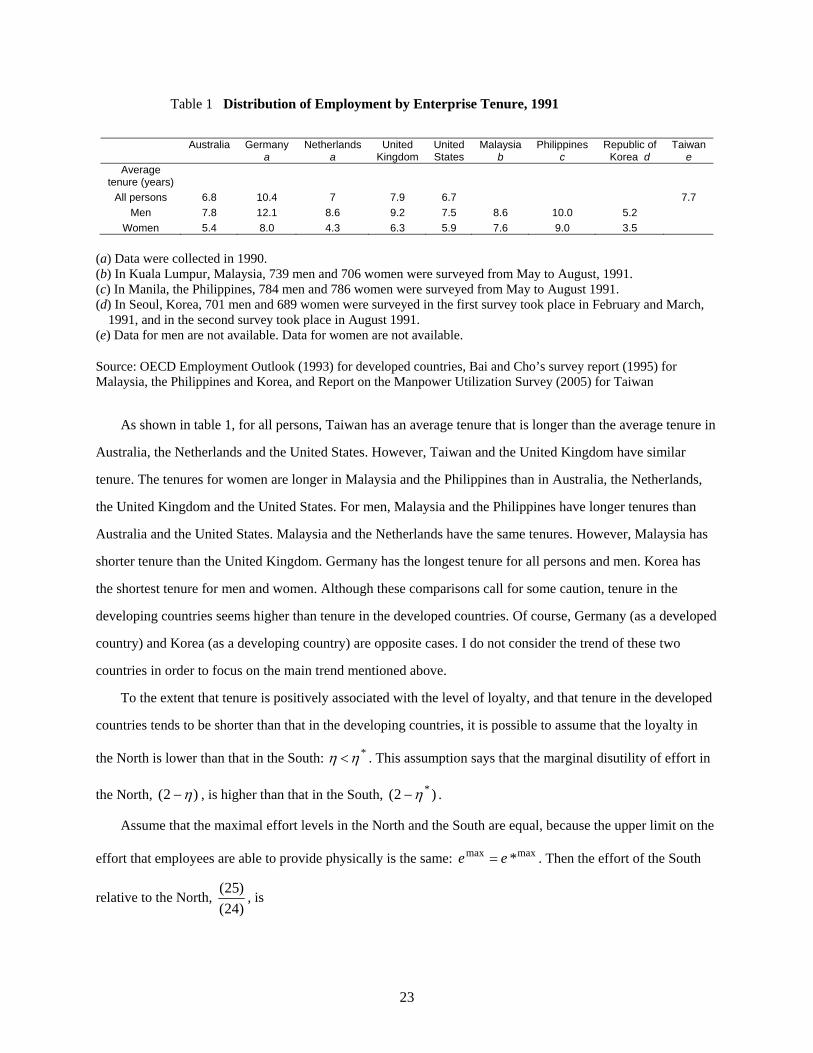
As shown in table 1, for all persons, Taiwan has an average tenure that is longer than the average tenure in

Australia, the Netherlands and the United States. However, Taiwan and the United Kingdom have similar

tenure. The tenures for women are longer in Malaysia and the Philippines than in Australia, the Netherlands,

the United Kingdom and the United States. For men, Malaysia and the Philippines have longer tenures than

Australia and the United States. Malaysia and the Netherlands have the same tenures. However, Malaysia has

shorter tenure than the United Kingdom. Germany has the longest tenure for all persons and men. Korea has

the shortest tenure for men and women. Although these comparisons call for some caution, tenure in the

developing countries seems higher than tenure in the developed countries. Of course, Germany (as a developed

country) and Korea (as a developing country) are opposite cases. I do not consider the trend of these two

countries in order to focus on the main trend mentioned above.

To the extent that tenure is positively associated with the level of loyalty, and that tenure in the developed

countries tends to be shorter than that in the developing countries, it is possible to assume that the loyalty in

the North is lower than that in the South: * . This assumption says that the marginal disutility of effort in

the North, )2( , is higher than that in the South, )2( * .

Assume that the maximal effort levels in the North and the South are equal, because the upper limit on the

effort that employees are able to provide physically is the same: maxmax *ee . Then the effort of the South

relative to the North, )24(

)25(, is

Australia

Germany

a Netherlands

aUnited

Kingdom United States

Malaysia b

Philippines c

Republic of Korea d

Taiwan e

Average tenure (years)

All persons 6.8 10.4 7 7.9 6.7 7.7

Men 7.8 12.1 8.6 9.2 7.5 8.6 10.0 5.2 Women 5.4 8.0 4.3 6.3 5.9 7.6 9.0 3.5

24

2*

**

)2

2(

)(

)(

w

w

me

me, where )2( > )2( * . (26)

This equation does not include the number of total stages m . That is, a change in the total number of stages

does not influence the relative effort since the Northern effort and the Southern effort are influenced by the

same total number of stages. Since 1)2

2(

*

, (26) implies that

)()( *

*

me

w

me

w .

This says that the wage per unit of effort in the North is higher than the wage per unit of effort in the South.

Thus the Northern firm has an incentive to shift production stages to the South.

[2-2-2] Northern Firm’s Cost under International Fragmentation

The Northern firm’s cost under international fragmentation is first explained. Assume that the firm locates

the stages with stage number n , n ,0( ]n̂ , in the North, and the stages with stage number *n ,

,0( ** n ]n̂m , in the South.21 The firm faces the headquarters costs and production costs occurred in the

North and the South, respectively. Let me explain the headquarters cost incurred by the n̂ Northern stages.

Since the headquarters remains in the North and employs Northern labor, the unit headquarters cost, fhc , is

obtained by substituting n̂ for n in (10’).

max

ˆ

e

nwhc f

, where N

. (27)

I explain production in the North. Under international fragmentation, effort and labor productivity are

affected by the total number of stages m . The production function for the Northern stages n ,0( ]n̂ is

derived by substituting )(me for )(ne in the production function (2) in national fragmentation, fnl for nl , and

)(mb for )(nb :

,min{ 1 nn zz })(

)(

mb

lme fn . (28)

Using (3’), the unit production cost at the n̂ th stage changes to

21 I take n̂ and m as exogenous variables for the moment. However, in the subsequent analysis, m and n̂ will be determined endogenously by the firm’s optimal choice.

25

)(

)(ˆˆ

me

wmbnpcn . (29)

From (27) and (29), the unit total cost at the n̂ th stage is

)(

)(ˆˆmaxˆˆ me

wmbn

e

nwpchctc n

ffn

. (30)

The headquarters in the North also manages the )ˆ( nm Southern stages. It employs Northern labor and

faces the headquarters cost incurred by the Southern stages. The headquarters faces more difficulty operating

the Southern stages than the Northern stages for a given number of stages, because of the smaller network size

and border barrier in the South. This causes the unit headquarters cost to be higher for the Southern stages than

for the Northern stages.

I evaluate the headquarters cost for the Southern stages for simplicity on the basis of )(N

, which

consists of the Northern network N and the input requirement of effective Northern labor for providing the

headquarters services for the Northern stages. This cost is denoted as *fhc . However, the small Southern

network and the high Southern border barriers lower the firm’s efficiency. The lower efficiency should be

embedded in this unit headquarters cost. I formalize this by defining *fhc as a two-part functional form. The

first part is linear with respect to and the number of the Southern stages, respectively: max

)ˆ(

e

wnm . The

second part is expressed as an increasing marginal cost of the Southern stages, max

)ˆ(

e

wnm . The parameter

, 0 , reflects an increase in the headquarters cost due to the small Southern network. Also, the parameter

, 1 , reflects an increase in the headquarters cost due to the high Southern border barriers.

max* })ˆ()ˆ({

e

wnmnmhc f

, where 0 , 1 . (31)

Before addressing the production cost for the Southern stages such that ,0( ** n ]n̂m , I look at the

production function for the Southern stages. The first stage in the South is denoted by )1ˆ( *n . This stage

uses intermediate good nZ ˆ which the n̂ th stage in the North produces, and employs Southern labor fn

l *1ˆ.

Since the Southern stage is one part of the production process of m stages, the productivity of labor in the

26

South depends on m , and is the same as in the North. The production function for the )1ˆ( *n th stage is

derived by substituting *1ˆnz for nz in (28), nz ˆ for 1nz , )(* me for )(me and fn

l *1ˆ for f

nl ,

nn zz ˆ1ˆ min{* , })(

)( *1ˆ*

mb

lme fn . (32)

Suppose that output of this stage is *1ˆnz . Then the )1ˆ( *n th stage uses *1ˆnz units of the intermediate nZ ˆ

in the South. The n̂ th stage produces *1ˆnz units of nZ ˆ : *1ˆˆ nn zz . Since the production of one unit of nZ ˆ

uses )(

)(ˆ

me

mbn units of Northern labor, *1ˆnz units of nZ ˆ embodies Northern labor of

)(

)(ˆ *1ˆ

me

zmbn n units. The

)1ˆ( *n th stage also uses Southern labor )(

)(*

1ˆ1ˆ

*

*

me

zmbl nfn

for the production of *1ˆnz units of *1ˆnZ . The

total labor input is the sum of embodied labor and the directly used labor: {)(

)(ˆ

me

mbn units of Northern labor +

)(

)(* me

mb units of Southern labor} *1ˆnz . The expression in the curly brackets is the total labor input per unit of

*1ˆnZ .

Consider the second stage in the South. The production function at the )2ˆ( *n th stage is

,min{ ** 1ˆ2ˆ nn zz })(

)( *2ˆ*

mb

lme fn .

I apply here the same logic as applied for the )1ˆ( *n th stage. For the production of *2ˆnz units of *2ˆnZ , the

)2ˆ( *n th stage uses *2ˆnz units of *1ˆnZ . And *2ˆnz units of *1ˆnZ embodies labor by {)(

)(ˆ

me

mbn units of

Northern labor + )(

)(* me

mb units of Southern labor} *2ˆnz since the total labor input per output of *1ˆnZ is

{)(

)(ˆ

me

mbn units of Northern labor +

)(

)(* me

mb units of Southern labor}. The Southern labor used for the

)2ˆ( *n th stage is )(

)(*

2ˆ2ˆ

*

*

me

zmbl nfn

. The total labor used for the )2ˆ( *n th stage is the sum of the

27

embodied labor and the labor used for this stage: {)(

)(ˆ

me

mbn units of Northern labor +

)(

)(2* me

mb units of Southern

labor} *2ˆnz . The expression in the curly brackets is the total labor input per unit of *2ˆnZ .

Applying this logic to the )ˆ( *nn th stage, the total labor used for the production of *ˆ nnz units of

*ˆ nnZ is {)(

)(ˆ

me

mbn units of Northern labor +

)(

)(*

*

me

mbn units of Southern labor} *ˆ nnz . The unit production cost

for the )ˆ( *nn th stage is obtained from the product of wage and units of labor per unit of *ˆ nnZ .

)(

)(

)(

)(ˆ*

**

ˆ *

me

wmbn

me

wmbnpc f

nn

. (33)

The unit total cost at the )ˆ( *nn th stage is the sum of the two unit headquarters costs in (27) and (31),

plus the unit production cost in (33). For simplicity, assume that 2 . Rearranging,

)(

)(})ˆ()ˆ({

)(

)(ˆˆ*

**

max

2

maxˆ *

me

wmbn

e

wnmnm

me

wmbn

e

wntc f

nn

. (34)

The sum of the first term and the second term on the RHS of (34) is the cumulative unit total cost from the first

stage to the n̂ th stage. The sum of the third term and the fourth term is the cumulative unit total cost from the

)1ˆ( *n th stage to the )ˆ( *nn th stage.

[2-2-3] National Fragmentation versus International Fragmentation

The Northern firm changes its mode of production from national fragmentation to international

fragmentation if the unit total cost under international fragmentation is lower than the unit total cost under

national fragmentation.

To compare these unit total costs, I consider two cases. The first case is that the Northern firm locates all

n~

stages in the North. Recall that n~

is the optimal number of total stages under national fragmentation. In the

second case, I consider a deviation from equilibrium of national fragmentation: the firm locates the first

)1~

( n stages in the North and moves the n~

th stage to the South.22

22 This is suboptimal. Exclusively in this section, I consider this suboptimal state to confirm whether there is an incentive to split the stages across the borders. I will address in section [2-2-4] how the firm optimally splits the stages into the North and the South.

28

In the first case, since the n~

th stage is in the North, the production function for this stage is obtained by

(2). The production function of nZ ~ is ,min{ 1~~ nn zz }

)~

(

)~

( ~

nb

lnen . The unit production cost for the n

~th stage is

)~

(

)~

(~

ne

wnbn from (3’). The unit headquarters cost for all n

~ stages is

max

~

e

nw from (10’), where

N

. The unit

total cost for the n~

th stage is the sum of these two costs:

max

~

e

nw+

)~

(

)~

(~

ne

wnbn. (35)

Turning to the second case, the firm keeps )1~

( n stages in the North and shifts one stage to the South.

First, I address the size of the employment pool since this may be affected by the shift of one stage. If the shift

takes place, the cost for the final stage n~

in the North under national fragmentation and the cost for the final

stage n~

in the South under international fragmentation will diverge, while the cost for the first )1~

( n stages

have remained the same. However, the difference between the two costs is very small compared with the total

cost covering all the stages under national fragmentation. The firm would not feel the necessity to adjust the

size of the pool in order to internalize the difference between the two costs for the final stage. I assume that the

sizes of the pool for national fragmentation and international fragmentation would be the same, l .

The production function for the Southern stage is obtained by replacing n̂ in (32) with )1~

( n :

,min{ 1~

1)1~

( * nn zz })

~(

)~

( *1)1~

(*

nb

lne fn

. One unit of *1)1~

( nZ is produced with )

~(

)~

()1~

(

ne

nbn units of Northern

labor and )

~(

)~

(* ne

nb units of Southern labor. Using the first term on the RHS of (33), the unit production cost for

the )1~

( n th stage in the North is )

~(

)~

()1~

(

ne

wnbn . The unit headquarters cost for the )1

~( n stages in the

North is max

)1~

(

e

wn from (27). Using the second term on the RHS of (33), the unit production cost for the

first stage in the South is )

~(

)~

(*

*

ne

wnb. Substituting )}1

~(

~{ nn for )ˆ( nm in (31), the unit headquarters cost

29

for only the first stage in the South is max

)(

e

w. Then the unit total cost for the n

~th stage is the sum of these

four costs:

})()1

~(

{maxmax e

w

e

wn

+ }

)~

(

)~

(

)~

(

)~

()1~

({

*

*

ne

wnb

ne

wnbn

. (36)

In order for the Northern firm to shift the n~

th stage to the South, the cost in (36) should be lower than the

cost in (35). In both cases, the unit total costs up to the )1~

( n th stage are the same. Thus, the difference

between the unit total cost for all the stages n~

in the first case and that for all the stages n~

in the second case

comes from the difference between the unit total cost for the n~

th stage in the North and the unit total cost for

the n~

th stage in the South. For simplicity, assuming that 1 , the condition for international fragmentation,

0)35()36( , is identical to the following condition:23

< })2

2(1{ 2

*

<1. (37)

I assume that the model satisfies this condition.

[2-2-4] Optimal Determination of International Fragmentation

The Northern firm determines the optimal number of total stages and split these optimally between the

North and the South as a way of incurring the lowest total cost. For the moment, assume that there is a number

of total stages across both regions, m , minimizing the unit total cost. For a given m , the firm locates n̂ stages

in the North and the other )ˆ( nm stages in the South. The unit total cost function for the final stage m is

obtained by replacing *n in (34) with )ˆ( nm .

])(

)()ˆ(})ˆ()ˆ({[}

)(

)(ˆˆ{

*

*

max

2

max)ˆ(ˆme

wmbnm

e

wnmnm

me

wmbn

e

wntc f

nmn

,

where w

dm

me

mb 2

)(

)( ,

*

2*

* )(

)(

w

md

me

mb ,

fled 2max )2( , fled 2*max* )2( , *dd since * . (38)

This is simplified as

23 See Appendix 2.

30

2*2max

)}ˆ(ˆ{})ˆ({ mnmdndnmme

wtc f

m . (39)

For the minimization of this cost with respect to n̂ for a given m , the first derivative with respect to n̂ is zero

and the second derivative is positive.

0)()ˆ(2

ˆ2*

max

mdd

e

nmw

n

tc fm

,

2

2

n̂

tc fm 0

2max

e

w. (40)

The number of Northern stages, n̂ , is obtained from (40).

2max

* )2

)(()(ˆ mw

eddmmn

. (41)

Since n̂ is a function of m , (39) is re-expressed as

2*2max

)}](ˆ{)(ˆ[])}(ˆ{[ mmnmdmndmnmme

wtc f

m . (39’)

The number of total stages is obtained by minimizing fmtc (39’) with respect to m . For the cost minimization,

the first derivative is zero and the second derivative is positive. For a given w , the first derivative is

0})(

{ 52*max

2max

m

w

ddedm

e

w

m

tc fm

.24 (42)

The second derivative is positive:

0})(5

{2 62*max

32

2

mw

ddedm

m

tc fm

, where .)

2

)(5( 3

12*max

wd

ddem

25 (43)

The optimal number of total stages is determined by (42). However, for graphical analysis, I rewrite (42)

as a new expression with A and B that are defined as follows.

0 BA , where 52*max

max}

)({

mw

dde

e

wA

, 2 dmB . (44)

The optimal number of total stages m~ is determined where BA . The shapes of A and B are monotonic in

m . The slope of A is flatter than that of B .26 As m becomes small, the value of A becomes smaller than

24 See Appendix 3.

25 For the second derivative in (43) to be positive, 0})(5

2{ 62*max

3

mw

ddedm

. Since the final stage m is

a positive number, 06 m . })(5

2{2*max

3

w

ddedm

has to be positive. Thus, 3

12*max

}2

)(5{

wd

ddem

.

31

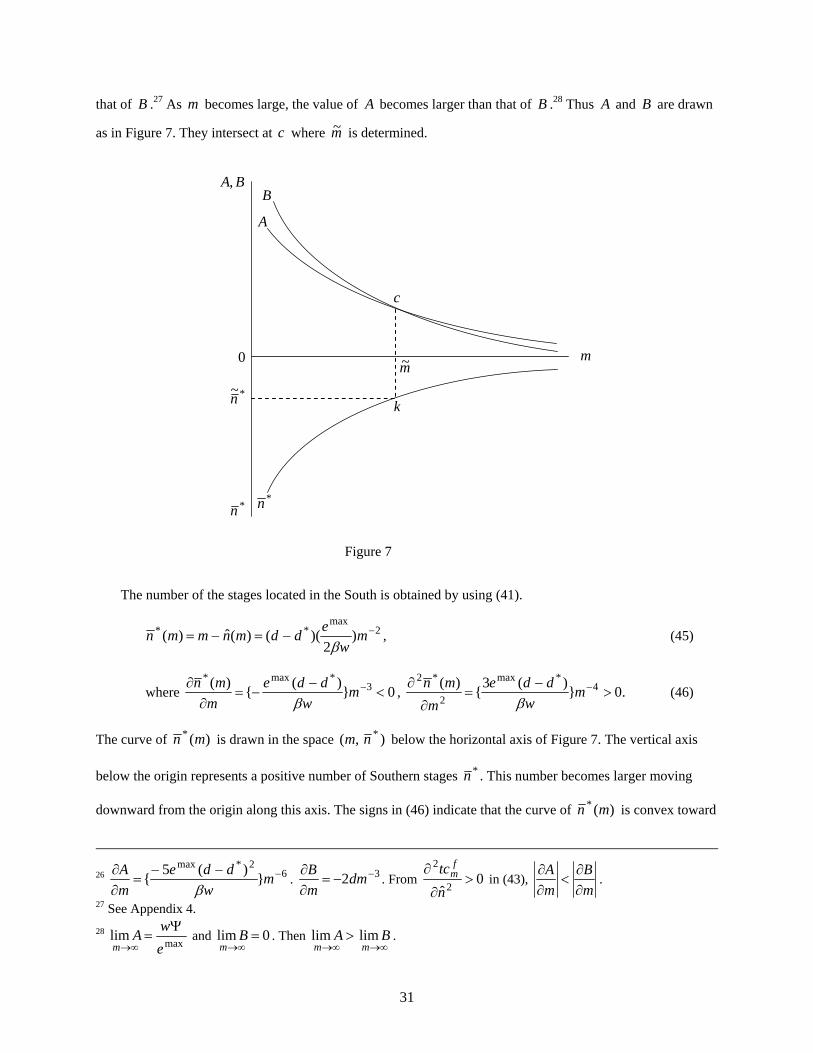
that of B .27 As m becomes large, the value of A becomes larger than that of B .28 Thus A and B are drawn

as in Figure 7. They intersect at c where m~ is determined.

Figure 7

The number of the stages located in the South is obtained by using (41).

2max

** )2

)(()(ˆ)( mw

eddmnmmn

, (45)

where 0})(

{)( 3

*max*

mw

dde

m

mn

, .0}

)(3{

)( 4*max

2

*2

mw

dde

m

mn

(46)

The curve of )(* mn is drawn in the space ,(m )*n below the horizontal axis of Figure 7. The vertical axis

below the origin represents a positive number of Southern stages *n . This number becomes larger moving

downward from the origin along this axis. The signs in (46) indicate that the curve of )(* mn is convex toward

26 62*max

})(5

{

mw

dde

m

A

. 32

dmm

B. From 0

ˆ 2

2

n

tc fm in (43),

m

B

m

A

.

27 See Appendix 4.

28 max

lime

wA

m

and 0lim

mB . Then

mAlim

mBlim .

m

*n

A

B

0

c

*n

k

BA,

m~

*~n

32

the origin in the space ,(m )*n . This can be understood as follows. As the total number of stages m increases,

the effect of the increasing returns to the labor division increases, and thus the production cost falls; the firm

has a smaller incentive for shifting the stages to the South to reduce the production cost; and this means that

the number of Southern stages *n decreases with the total number of stages m . The optimal number of

Southern stage, *~n , is determined at k where the vertical line extended downward from the point c touches

the curve )(* mn .

I have to mention the possibility that the headquarters remains in the North and all production stages shift

to the South. The possibility of this case is very low in the model, but this case can also be ruled out if *

satisfies )22(2

* .29

[2-2-5] Effect of International Fragmentation on the Total Number of Stages

I address what happens to the total number of stages when the firm changes its mode of production from

national fragmentation to international fragmentation. I compare the total number of stages in national

fragmentation n~

to that in international fragmentation m~ .

The curves A and B in Figure 7 are used for this purpose. First, consider a point on the horizontal axis

which is located at m~ . Where m is equal to m~ , the values of A and B are represented by ,c and are the

same.

1)(

)(

mB

mA, where mm ~ . (47)

Second, consider a point on the left of m~ on the horizontal axis. Where mm ~0 , the value on the curve A

corresponding to this point is smaller than the value on the curve B in Figure 7. Using (47),

1)~(

)~(

)(

)(

mB

mA

mB

mA, where mm ~0 . (48)

Third, consider a point on the right of m~ , that is, mm ~ . The value on A corresponding to this point is larger

than the value on B in Figure 7. By (47),

1)~(

)~(

)(

)(

mB

mA

mB

mA, where mm ~ . (49)

29 See Appendix 5.

33

Using )(mA and )(mB in (44), )(

)(

mB

mA is obtained as follows.

})(

{1

)(

)( 32*max

max

2

w

mdde

e

mw

dmB

mA

.30 (50)

This ratio is used to compare m~ and n~

. If m has the same number as the equilibrium number of total stages

in national fragmentation n~

, this ratio is expressed as )

~(

)~

(

nB

nA. If

)~

(

)~

(

nB

nA is less than or equal to one, this implies

that mn ~~ from (47) and (48):

1)~(

)~(

)~

(

)~

(

mB

mA

nB

nA mn ~~ . (51)

If )

~(

)~

(

nB

nA is larger than one, this implies that mn ~~ from (49):

1)~(

)~(

)~

(

)~

(

mB

mA

nB

nA mn ~~ . (52)

To find the value of )

~(

)~

(

nB

nA, substitute n

~ for m in (50). Using n

~ in (23), 1 and 1 ,

])()2(

})2()2{(1[

)~

(

)~

(

23

21

21

23

25max

22*2

Nl

lle

w

l

l

nB

nA

f

f

,31 where 10 * . (53)

The second term in the square brackets on the RHS in (53) is positive. The value in the square brackets is

larger than one. Thus, whether the value of )

~(

)~

(

nB

nA is larger than one or not depends on the size of the

employment pool in national fragmentation relative to that in international fragmentation, fl

l. The following

cases are considered.

(i) case: fl l

If the size of the employment pool with international fragmentation is less than or equal to that with

national fragmentation, the ratio of employment is 1fl

l. The RHS in (53) is the product of the ratio

fl

l and

30 See [A6-1] in Appendix 6. 31 See [A6-5] in Appendix 6.

34

the value in the square brackets. The product is larger than one, so that the LHS is larger than one: 1)

~(

)~

(

nB

nA.

This occurs, as explained in (52), where mn ~~ .

This can be explained as follows. The internationally fragmented firm faces a low Southern wage as well

as a high Northern wage, but the nationally fragmented firm faces only a high Northern wage. The number of

workers hired by the internationally fragmented firm is smaller than or equal to that hired by the nationally

fragmented firm. Thus the former firm faces a lower production cost than the latter firm.32 The internationally

fragmented firm feels less pressure to reduce the production cost compared with the nationally fragmented firm.

The former firm has a smaller incentive to increase the total number of stages so as to raise their productivity

than the latter firm. This says that the total number of stages should be smaller in international fragmentation

than in national fragmentation.

(ii) case: fl l

If the size of the employment pool is larger with international fragmentation than with national

fragmentation, the ratio of employment is 1fl

l. The RHS in (53) is the product of the ratio

fl

l and the

value in the square brackets, where the former is smaller than one and the latter is larger than one. According

to which one dominates, the value of the product is greater than, equal to or less than one. Thus, the value of

the LHS in (53) is 1)

~(

)~

(

nB

nA. This implies that mn ~~

from (51) and (52).

Intuitively, the internationally fragmented firm in comparison to the nationally fragmented firm faces a

lower wage, but hires a larger number of workers. This could cause the production cost with international

fragmentation to be larger than, equal to or smaller than the production cost with national fragmentation. Thus,

it is difficult to say which firm has a greater incentive to reduce its production cost. Therefore, the total number

of stages with international fragmentation could be larger than, equal to or smaller than that with national

fragmentation.

32 The total cost – the sum of the headquarters cost and the production cost – is affected by the network size, loyalty, border barrier, size of employment pool and wage. The degree of segmentation of the production process is determined by the minimization of the total cost. These factors are reflected on the RHS in (53). Since the value in

the square brackets on the RHS is larger than one, whether or not )

~(

)~

(

nB

nA is larger than one is determined by the ratio

of the numbers of workers hired by the two firms. That is, the second term in the square brackets, which includes the factors mentioned, does not play a key role in determining whether the value of the ratio in (53) is larger than one. Therefore, I focus on the wage cost of production.

35

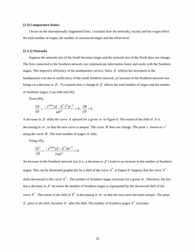
[2-3] Comparative Statics

I focus on the internationally fragmented firm. I examine how the networks, loyalty and the wages affect

the total number of stages, the number of outsourced stages and the effort level.

[2-3-1] Networks

Suppose the network size of the South becomes larger and the network size of the North does not change.

The firm connected to the Southern network can communicate information faster and easily with the Southern

stages. This improves efficiency of the headquarters service. Since reflects the increment in the

headquarters cost due to inefficiency of the small Southern network, an increase in the Southern network size

brings on a decrease in . To examine how a change in affects the total number of stages and the number

of Southern stages, I use (44) and (45).

From (44),

A

0)(

2

52*max

w

mdde, 0B

.

A decrease in shifts the curve A upward for a given m in Figure 8. The extent of the shift of A is

decreasing in m , so that the new curve is steeper. The curve B does not change. The point c moves to c

along the curve B . The total number of stages m falls.

Using (45),

*n0

2

)(2

2*max

w

mdde.

An increase in the Southern network size (i.e., a decrease in ) leads to an increase in the number of Southern

stages. This can be illustrated graphically by a shift of the curve *n in Figure 8. Suppose that the curve *n

shifts downward to the curve '*n . The number of Southern stages increases for a given m . Therefore, the fact

that a decrease in increases the number of Southern stages is represented by the downward shift of the

curve *n . The extent of the shift of *n is decreasing in ,m so that the new curve becomes steeper. The point

k , prior to the shift, becomes k after the shift. The number of Southern stages *n increases.

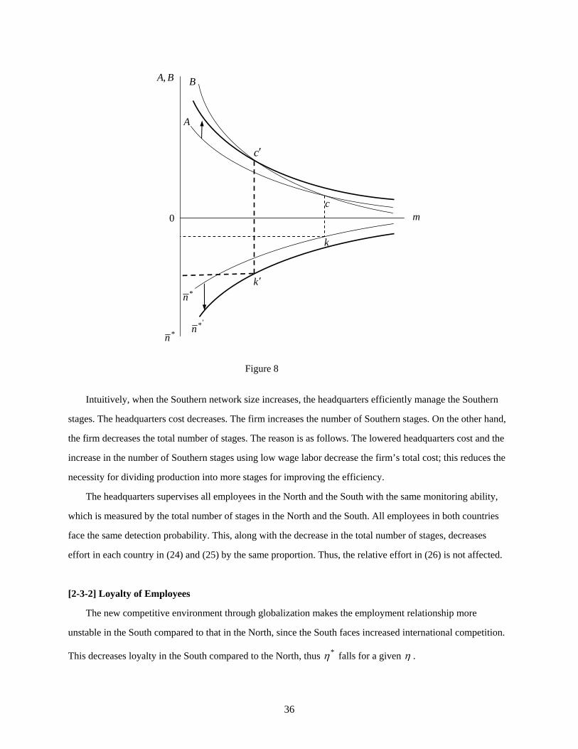
36

Figure 8

Intuitively, when the Southern network size increases, the headquarters efficiently manage the Southern

stages. The headquarters cost decreases. The firm increases the number of Southern stages. On the other hand,

the firm decreases the total number of stages. The reason is as follows. The lowered headquarters cost and the

increase in the number of Southern stages using low wage labor decrease the firm’s total cost; this reduces the

necessity for dividing production into more stages for improving the efficiency.

The headquarters supervises all employees in the North and the South with the same monitoring ability,

which is measured by the total number of stages in the North and the South. All employees in both countries

face the same detection probability. This, along with the decrease in the total number of stages, decreases

effort in each country in (24) and (25) by the same proportion. Thus, the relative effort in (26) is not affected.

[2-3-2] Loyalty of Employees

The new competitive environment through globalization makes the employment relationship more

unstable in the South compared to that in the North, since the South faces increased international competition.

This decreases loyalty in the South compared to the North, thus * falls for a given .

m

*n

A

B

'*n

0

c

c

*n

k

k

BA,

37

To investigate how a decrease in * influences the total number of stages, (44) is used.

0)}()(2

{*

*5*max

*

d

w

mddeA, 0)(

*2

*

d

mB

,

where 0)2(2 *max*

*

fled

, 0*

d

from (38). (54)

This says that only the curve A shifts downward as * falls for a given m as in Figure 9. Since the extent of

the shift of A is decreasing in m , the new curve becomes less steep. The curve B does not change. The point

c moves to c along the curve B . The total number of stages m increases.

Figure 9

The effect of a decrease in * on the number of Southern stages is obtained from (45).

0))(2

(*

*2max

*

*

d

w

men, where 0

*

*

d

in (54).

m

*n

A

B

'*n

0

c

c

*n

k

k

BA,

38

A fall in Southern loyalty leads to a decrease in the number of Southern stages. This can be illustrated by a

upward shift of the curve *n since the number of Southern stages decreases for a given m . The extent of the

shift of *n is decreasing in m , so that the new curve becomes less steep. The point k shifts to k after the

curve *n shifts upward to the curve '*n . The number of Southern stages *n decreases.

If Southern loyalty falls, its effect on Northern effort is from (24):

0)2(

)(*2max*

m

le

wmef

, where 0*

m

. (55)

The negative signs in (55) can be explained as follows. The fallen Southern loyalty increases the total number

of stages (i.e., 0*

m

); this increases the firm’s detection probability and thus Northern effort rises.

The effect on Southern effort of lower Southern loyalty is from (25):

0})2()2(

2{

)(*2*max

*

3*max

*

*

*

m

le

w

le

mwmeff

, where maxmax* ee .

The first term in the curly brackets is positive. This says that lowered Southern loyalty leads to a fall in

Southern effort, given that m does not change. The second term in the curly brackets is negative; the increased

total number of stages increases the detection probability and thus Southern effort. These opposite movements

make the effect on Southern effort ambiguous.

I now examine the relationship between Southern loyalty and relative effort. From (26),

0}

)2

2(

]{)

2

2(

})(

)({

[

})(

)({

*

*

*

*

*

*

me

me

me

me

, (56)

where 0)2

2)((2]

)2

2(

})(

)({

[*

*

*

*

w

wme

me

, 0)2(

)2(]

)2

2(

[2**

*

.

The positive sign in (56) implies that a fall in * causes a fall in *2

2

and thus a fall in

)(

)(*

me

me. Thus,

lowered Southern loyalty reduces Southern effort relative to Northern effort.

These results are explained intuitively. If loyalty in the South falls relative to the North, the South’s

relative disutility of effort rises. The employees in the South provide less effort relative to the employees in the

39

North. This increases the production cost of outsourced stages. The firm decreases outsourcing to the South

and brings back some of the Southern stages to the North. The increase in Northern stages using high wage

labor, and the lowered Southern effort, increase the total cost. To improve the efficiency of production, the

firm increases the total number of stages.

[2-3-3] Wages

Suppose that the Southern wage rises for a given Northern wage. 33 The change in the relative wage does

not affect the position of the curves A and ,B since A and B in (44) have no Southern wage term:

0**

w

B

w

A. This says that the total number of stages m is not changed by the Southern wage. The effect

on the number of Southern stages *n is from (45): 0*

*

w

n. The number of Southern stages is not affected by

the Southern wage.

If the Southern wage rises, Southern effort increases and Northern effort does not change.

0})2(

1{

)(2*max*

*

fl

m

ew

me

, 0

)(*

w

me.34

Also, a rise in the wage of the South relative to the North increases the effort of the South relative to the North.

From (26),

0)2

2(

)(

})(

)({

2**

*

w

w

me

me

. (57)

These results can be understood as follows. The rise in the Southern wage increases Southern employees’

effort. This relatively decreases the production cost in the South. At the same time, the increased wage raises

the production cost in the South. These opposite effects are traded off, and the degree of outsourcing is not

changed. Also, the total number of stages is not changed.

33 I treat the wages as exogenously given. However, it has also become an important issue how wages are affected by international fragmentation. In the single sector H-O model with skilled and unskilled labor of Deardorff (2005), the services outsourcing of skilled-labor from the developed country (the North) causes the wage of unskilled labor in the North to fall below that in the developing country (the South), if the North continues to diversify. However, the high-skilled and low-skilled labor in the North gains if specialization occurs due to largely different factor endowments. Also, Grossman and Rossi-Hansberg (2009) examine how falling costs of offshoring affect high-skill and low-skill wages in the source country in a H-O model with two sectors. They show that offshoring benefits the factors whose tasks are moved more easily overseas and generates shared gains for all domestic factors. 34 See Appendix 7.

40

I consider another case of a rise in the Northern wage for a given Southern wage. The direction of shift of

the curve A depends on the values of parameters, while the curve B does not change:

2

52*max

max

)(

w

mdde

ew

A

0 , 0

w

B.

The direction of movement of m is ambiguous, so that the change in the total number of stages is ambiguous.

The effect on the number of Southern stages *n is

)21

(2

)(2

*max*

w

m

mwwm

dde

w

n

0 , where

w

m0.

The number of Southern stages can decrease, increase or not change, since *n depends on the change in m

with respect to w .

When the Northern wage rises, the changes in effort in both regions are ambiguous due to the ambiguity

of the change in the total number of stages. This is shown by using (24) and (25).

To examine how the rise in the Northern wage affects Northern effort relative to Southern effort, I use (57).

This indicates that a decrease in the ratio of the Southern wage to the Northern wage w

w*

leads to a decrease

in the ratio of Southern effort to Northern effort )(

)(*

me

me. Since a decrease in

w

w*

means an increase in *w

w,

and since a decrease in )(

)(*

me

me means an increase in

)(

)(* me

me, an increase in

*w

w leads to an increase in

)(

)(* me

me. In other words, a rise in the Northern wage for a given Southern wage causes a rise in Northern effort

relative to Southern effort.

Now I explain intuitively why the changes in the total number of stages and outsourcing with respect to a

change in the Northern wage are ambiguous. A rise in the Northern wage increases Northern employees’ effort

relative to Southern employees’ effort. This relatively decreases the production cost in the North. At the same

time, the increased wage raises the headquarters cost and the production cost in the North. These work in

opposite directions, so that the total cost can increase, decrease or not change. Thus, the effect of the increased

Northern wage on the total number of stages is ambiguous. Since this ambiguity influences production costs of

both Northern stages and Southern stages, the comparison of production costs between the North and the South

is also difficult. This causes the effect on outsourcing to be ambiguous.

41

[3] Conclusion

This paper addresses how physical networks, loyalty of workers and wages affect international

fragmentation and the work effort, in a world consisting of a developed country and a developing country.

Splitting a single production process into multiple-stages increases a headquarters’ monitoring ability to find

where shirking occurs. This increases the employees’ work effort. The firm has an incentive to fragment

production. However, since the headquarters cost for coordinating and monitoring the stages increases with the

number of production stages, this limits the number of total stages. The international differences in the network

sizes, border barriers, loyalty and wages cause the stages to be separated into the North and the South. The

Northern firm determines the optimal number of total stages as a way of incurring the lowest total cost.

When the mode of production changes from national fragmentation to international fragmentation, if

international fragmentation brings on a decrease in employment, the internationally fragmented firm compared

with the nationally fragmented firm faces low wage and decreased employment. This weakens the

internationally fragmented firm’s incentive to improve efficiency by increasing the total number of stages, thus

leading to a decrease in the total number of stages. However, if international fragmentation brings on an

increase in employment, this raises the incentive to improve efficiency by increasing the total number of stages.

On the contrary, the low wage weakens this incentive. These opposite effects make the effect of international

fragmentation on the total number of stages ambiguous.

An increase in the Southern network decreases the headquarters cost for the Southern stages compared to

the headquarters cost for the Northern stages. This increases outsourcing from the North to the South. Since

the increased Southern network reduces the firm’s cost, the necessity for the division of production is

diminished. The firm decreases the total number of stages. Since all employees in both regions face a lowered

and identical detection probability, this decreases the level of effort in the North and the South, and keeps the

effort of the South relative to the North unchanged.

The new competitive environment through globalization makes employment relationships more unstable

in the South compared to that in the North, since the South is under more protection that limits free trade. As a

result, Southern employees’ loyalty falls and their effort relative to the Northern employees’ effort decreases.

This increases the production cost in the South and reduces outsourcing. However, the firm increases the total

number of stages to improve productivity.

If the Southern wage rises, Southern effort increases, but Northern effort does not change. The increasing

effort in the South decreases the production cost in the South. However, a rise in the Southern wage could also

42

increase the production cost in the South. These opposite effects on the production cost are traded off, so

outsourcing does not change. Also, the total number of stages is not changed.

If the Northern wage rises, the headquarters cost and the production cost in the North increase. At the

same time, the risen Northern wage increases Northern effort relative to Southern effort. This decreases the

production cost in the North. The effect of the risen wage and the effect of the risen effort work in opposite

directions, so outsourcing is determined by which of these effects dominates. The effect of the risen Northern

wage on outsourcing is ambiguous. The effect of the risen Northern wage on the total stages is also ambiguous.

[References]

Asian Development Bank, 1992. Key Indicators of Developing Member Countries of ADB. Bai, Moo Ki and Cho, Woo Hyun, 1995. Employment Structures in Manufacturing of Four Surveyed Countries and terms of Female Employment in Women’s Wages and Employment in Korea. Seoul: Seoul National University Press. Becker, G. and Murphy, K., 1992. The Division of Labor, Co-ordination costs, and Knowledge. Quarterly Journal of Economics, 107. Brecher, Richard A., 1992. An Efficiency-Wage Model with Explicit Monitoring: Unemployment and Welfare in an Open Economy. Journal of International Economics, 32. Calvo, Guillermo A. and Wellisz Stanislaw, 1978. Supervision, Loss of Control, and the Optimum Size of the Firm. The Journal of Political Economy, 86. Copeland, Brian R., 1989. Efficiency Wages in a Ricardian Model of International Trade. Journal of International Economics, 27. Deardorff, Alan V., 2001 a. Trade and Welfare Implication of Networks. Paper prepared for the Murray S. Johnson Conference on International Economics, University of Texas. Deardorff, Alan V., 2001 b. Fragmentation in Simple Trade Models. North American Journal of Economics and Finance, 12. Deardorff, Alan V., 2005. A Trade Theorist’s Take on Skilled-Labor Outsourcing. International Review of Economics and Finance, 14. Directorate-General of Budget, 2005. Accounting and Statistics, Executive Yuan, Report on the Manpower Utilization Survey in Taiwan Area. Republic of China. Edwards, Brian K. and Starr, Ross M., 1987. A Note on Indivisibilities, Specialization, and Economies of Scale. The American Economic Review, 77. Either, Wilfred J., 1979. Internationally Decreasing Costs and World Trade. Journal of International Economics, 9.

43

Freund, Caroline and Weinhold, Diana, 2002. The Internet and International Trade in Services. The American Economic Review, v.92 no.2. Grossman, Gene M. and Rossi-Hansberg Esteban, 2007. The Rise of Offshoring: It’s Not Wine for Cloth Anymore. Federal Reserve Bank of Kansas City on “The New Economic Geography: Effects and Policy Implications,” Jackson Hole Symposium. Grossman, Gene M. and Rossi-Hansberg Esteban, 2009. Trading Tasks: A Simple Theory of Offshoring. The American Economic Review, forthcoming. Harris, Richard G., 2001. A Communication-Based Model of Global Production Fragmentation, in Arndt, Sven W. and Henryk Kierzkowski (eds.) Fragmentation: New Production Patterns in the World Economy. Oxford: Oxford University Press. Leamer, Edward E., 1999. Effort, Wages, and the International Division of Labor. The Journal of Political Economy, 107. Lee, Kiong Hock and Sivananthiran, A., 1991. Report on Employment, Occupational Mobility and Earnings in the Kuala Lumpur Urban Labor Market with Special Reference to Women in the Manufacturing Sector: Draft. Matusz, Steven J., 1996. International Trade, the Division of Labor, and Unemployment. International Economic Review, 37. Minkler, Lanse, 2004. Shirking and Motivations in Firms: Survey Evidence on Worker Attitudes. International Journal of Industrial Organization, 22. National Bureau of Statistics, Economic Planning Board, Report on Mining and Manufacturing Census 1990, Republic of Korea. OECD, Employment Outlook 1993. Paris. Reichheld, Frederick F. and Teal, Thomas, 1996. The Loyalty Effect: The Hidden Force behind Growth, Profits and Lasting Value. Bain & Company, Inc. Harvard Business School Press. Sennett, Richard, 1998. Corrosion of Character: The Personal Consequences of Work in the New Capitalism. New York: W.W. Norton and Company, Inc. Shapiro, Carl and Stiglitz, Joseph E., 1984. Equilibrium Unemployment as a Worker Discipline Device. The American Economic Review, 74. Smith, Adam, 1937. The Wealth of Nations. New York: Modern Library; Orig. pub. 1776.

[Appendices]

[Appendix 1]

The maximal expected utility is obtained by solving the constrained maximization problem, which

maximizes EU subject to a single constraint such that max)( eee . To solve this problem, it should first

be checked whether the constraint qualification is satisfied. The condition of constraint qualification is as

follows. If the expected utility is maximized at an effort level e such that maxee , and if the constraint is

44

binding at e , then e

e

)(

should not be zero at e on the boundary of the constraint: 0)(

e

e. When I turn

to the maximization problem at hand, the constraint has the feature that 1)(

e

e for all e . This means that

0)(

e

e at a value of e on the boundary, so the constraint, max)( eee , satisfies the constraint

qualification. Then we are able to form the Lagrangian function and to calculate the optimal effort.

,(eL )() maxeeEU .

The first order conditions are

0

e

EU

e

L, [A1-1]

0)( max ee , [A1-2]

0 , [A1-3]

maxee . [A1-4]

If 0 in [A1-3], 0

e

EU from [A1-1] and 0)( max ee from [A1-2]. This means that maxee .

However, if 0 in [A1-3], 0

e

EU from [A1-1]. Then

e

EU

in (15) should be zero. The effort level is

determined at 2max

2

)2(

e

wPe .

The two effort levels, maxe and 2max

2

)2(

e

wPe , are candidates that can be considered in the range of

maxee in [A1-4]. The first candidate represents case )(iii in Figure 2. The second candidate represents the

case )(ii and max2max

2

)2(e

e

wPe

by [A1-4].

Compare the levels of expected utility at these candidates. First, substituting 2max

2

)2(

e

wPe into the

expected utility function in (14),

,0})1(2)2(

{max

2

wPe

wPEU

where 2)2(1 , 1)1(0 P . [A1-5]

45

Second, substituting maxee into (14),

0)2(2 max ewEU . [A1-6]

If [A1-6] is negative or zero, employees would provide effort 2max

2

)2(

e

wPe since [A1-5] is positive.

However, if [A1-6] is positive, the difference between [A1-5] and [A1-6] is positive:

0)}]2({[)2(

1 2maxmax

ewPe

.

This says that [A1-5] is larger than [A1-6]. Thus employees choose [A1-5] that yields the higher expected

utility. They provide effort 2max

2

)2(

e

wPe . Regardless of whether [A1-6] is negative, zero or positive, [A1-

5] is always larger than [A1-6]. Thus, case )(ii has higher expected utility than case )(iii .

[Appendix 2]

The condition that international fragmentation occurs is that 0)35()36( :

0})

~(

)~

(~~

{}])

~(

)~

(

)~

(

)~

()1~

({}

)()1~

([{

max*

*

maxmax

ne

wnbn

e

nw

ne

wnb

ne

wnbn

e

w

e

wn .

This is rearranged as

0})

~()

~(

){~

(*

*

max

ne

w

ne

wnb

e

w. [A2-1]

Using (18), where nn~ ,

n

le

ne

w~

)2(

)~

(

2max . [A2-2]

Recall that the sizes of the pool for national fragmentation and international fragmentation are assumed to be

the same, l . Using [A2-2],

n

le

ne

w~

)2(

)~

(

2*max

*

* . [A2-3]

For simplicity, I assume that 1 . From (1),

nnb ~

1)

~( . [A2-4]

Substituting [A2-2], [A2-3] and [A2-4] into [A2-1],

46

0})2()2({~2*2

2

max

max

n

le

e

w. [A2-5]

From (23), where 1 , 1 and N

, 2

12max

])}2({

[~

w

len

. Substituting n~

into [A2-5],

0}])2

2(1{[ 2

*

max

e

w. Since 0

max

e

w, 0}])

2

2(1{[ 2

*

. This means

})2

2(1{ 2

*

. Since 1N

in (9) and 1)

2

2(0

*

from (26), < })2

2(1{ 2

*

1.

[Appendix 3]

The first derivative of fmtc in (39’) with respect to m is

2*max

}])(ˆ

1{})(ˆ

{[}])(ˆ

1)}{(ˆ{2[

mm

mnd

m

mnd

m

mnmnm

e

w

m

tc fm

0)}](ˆ{)(ˆ[2 3* mmnmdmnd .

This is rearranged as

2**max

})(ˆ

){(}])(ˆ

1)}{(ˆ{2[

mdm

mndd

m

mnmnm

e

w

0})(ˆ){(2 3** mmdmndd . [A3-1]

Rearranging (41),

2max

* )2

)(()}(ˆ{ mw

eddmnm

. [A3-2]

The derivative of )(ˆ mn in (41) with respect to m is

3max

* ))((1)(ˆ

mw

edd

m

mn

. [A3-3]

Substituting (41), [A3-2] and [A3-3] into [A3-1],

}]))((}{)2

)({(2[ 3max

*2max

*max

mw

eddm

w

edd

e

w

m

tc fm

2*3max

** ]}))((1){[( mdmw

edddd

0]})2

)((){[(2 3*2max

** mmdmw

eddmdd

. [A3-4]

47

[A3-4] is rearranged as

})()({})()({ 5max

2*25max

2*max

mw

edddmm

w

edd

e

w

0})2

()({2 5max

2*2 mw

edddm

.

Then 0})(

{ 52*max

2max

m

w

ddedm

e

w

m

tc fm

.

[Appendix 4]

I need to prove that 0)( AB for a small value of m . Rearrange the second derivative in (43),

0})()(52{ 6max

2*3 mw

edddm

. Factoring out,

0})())(5.2({2 5max

2*21 mw

edddmm

.

Since 02 1 m , 0})())(5.2({ 5max

2*2 mw

edddm

. Rewriting this,

0})())(5.1()()({ 5max

2*5max

2*2 mw

eddm

w

edddm

. [A4-1]

From (44), })()({)( 5max

2*max

2

mw

edd

e

wdmAB

. Substituting this equation into [A4-1],

0])())(5.1(})[{( 5max

2*max

mw

edd

e

wAB

. Rearranging this,

)( AB > 5max

2*max

)())(5.1(

mw

edd

e

w

. [A4-2]

We want to know the sign of )( AB in the range left of m~ on the horizontal axis in Figure 7. This sign

is determined when the value on the RHS of [A4-2] is obtained. Thus, I calculate this value where m has a

value smaller than m~ , such that 1m as an example. That is

)())(5.1(max

2*max w

edd

e

w

. [A4-3]

Using the notations for d and *d in (38),

48

.)}]4)({([}])2()2{([)( 2**max22*2max2* ff leledd [A4-4]

Substituting [A4-4] and N

into [A4-3], [A4-3] is rewritten as

maxe

w]

)}4)({()5.1([

2

22**4max

w

le

N

f

. [A4-5]

I check the magnitudes of the two terms in the square brackets in [A4-5]. First, consider the numerators.

The parameter is the input requirement of effective labor per unit of headquarters service. fl is the total

labor input for the production process. Conceptually, should be smaller than fl : fl . Assume that

1max e . The conditions that 10 , 10 * and * make 1)(0 * and

4)4(2 * . I assume that )( * ensures that 1)}4)({()5.1( 2**4max fle . Since

fl , the relation between the two numerators in the square bracket is

< 22**4max )}4)({()5.1( fle .

Next, consider the denominators in the square brackets in [A4-5]. If the Northern network size N is

represented by the value of the network infrastructure, N is larger than 2w . Note that w is the wage per

worker. The condition in (37), 1 , makes that 22 ww . This yields that 2wN . Then the absolute

value of the first term in the square brackets in [A4-5] is smaller than the value of the second term:

N

<

2

22**4max )}4)({()5.1(

w

le f

.

This makes [A4-5] positive and thus [A4-3] is positive. This says that 0)( AB from [A4-2]. In other

words, AB in the left range of m~ .

[Appendix 5]

I have to check whether there is a case that the headquarters remains in the North and all production stages

shift to the South at the values of m which are determined by (42), in other words, at the values of m that are

determined by the intersection of the curves A and B . This case means that there is no production stage in the

North: 0)(ˆ mn . Substituting 0)(ˆ mn into (41), m is obtained. When I define it as m ,

3

1*max

}2

)({

w

ddem

. [A5-1]

49

If this extreme case exists, the condition in (42), 0

m

tc fm , should also be satisfied where mm .

0})(

{ 52*max

2max

H

mw

ddemd

e

w

.

If H is not zero, this extreme case does not exist. If H is zero, this extreme case can exist.

To check whether H is zero, rewrite H as follows.

}])(

{[1 2*max

35max5 w

ddemdm

e

w

m

. [A5-2]

Since 05 m , I should check whether the value in the square brackets is zero. Using [A5-1], the expression

in the square brackets of [A5-2] is rewritten:

}2

)()]{2(}

2

)({[

*max*3

2*max

max w

ddedd

w

dde

e

w

. [A5-3]

Since *dd in (38), 0}2

)({ 3

2*max

max

w

dde

e

w

and 0}

2

)({

*max

w

dde

. Then, from [A5-3], three cases

are considered.

)(i If 02 * dd , [A5-3] is non zero.

)(ii If 02 * dd and if *3

2*max

max2}

2

)({ dd

w

dde

e

w

, [A5-3] is non zero.

)(iii If 02 * dd and if *3

2*max

max2}

2

)({ dd

w

dde

e

w

, [A5-3] is zero.

The extreme case exists if case )(iii occurs.

I now explain the likelihood that case )(iii occurs, compared with the cases )(i and )(ii . The case )(iii

has more restrictive conditions than the case )(ii . The reason is that the situations satisfying the second

condition in )(iii , *3

2*max

max2}

2

)({ dd

w

dde

e

w

, occur less frequently than the situations satisfying the

second condition in )(ii . Also, case )(iii has more restrictive conditions than case )(i . Then the likelihood

that case )(iii can occur is lower than the cases )(i and )(ii . In fact, since the second condition in )(iii

50

consists of many parameters, it is very hard to find a combination of the values of the parameters that satisfy

the second condition in )(iii . Thus, the likelihood of case )(iii is very low.

Another way to avoid the extreme case is to assume that 02 * dd , like the condition in )(i . This

condition makes that )22(2

* , when fled 2max )2( and fled 2*max* )2( in (38)

are substituted into 02 * dd . Also this inequality ensures that 10 and 10 * .

[Appendix 6]

Using )(mA and )(mB in (44),

2

52*max

max}

)({

)(

)(

dm

mw

dde

e

w

mB

mA }

)({

1 32*max

max

2

w

mdde

e

mw

d

. [A6-1]

The ratio where nm~ ,

)~

(

)~

(

nB

nA, is obtained as follows. Substituting n

~ for m in [A6-1],

}~

)(~

{1

)~

(

)~

( 32*max

max

2

w

ndde

e

nw

dnB

nA

. [A6-2]

Using n~

in (23), 1 and 1 ,

21

])}2({

[~ 2max

w

lNen

. [A6-3]

From the definitions of d and *d in (38),

})2()2{()( 2*2max* fledd . [A6-4]

Substituting [A6-3] and [A6-4] into [A6-2],

])2()(

})2()2{()2(}[

)2(

1{

)~

(

)~

(3

22*222max

2max23

21

23

lN

wllNe

lenB

nA f

f

])()2(

})2()2{(1[

23

21

21

23

25max

22*2

Nl

lle

w

l

l

f

f

. [A6-5]

51

[Appendix 7]

Using (25), }1

)2()2(

1{

)(*2*max*

*

2*max**

*

w

m

le

w

l

m

ew

meff

. Since maxmax* ee and

0*

w

m, 0}

)2(

1{

)(2*max*

*

fl

m

ew

me

.

Using (24), *2max*

})2(

{)(

w

m

le

w

w

mef

. Since 0

*

w

m, 0

)(*

w

me.