international corporation air sciences€¦ · · 2001-09-07international corporation air...

International Corporation Air Sciences

Final Report

ENHANCED METEOROLOGICAL MODELING AND PERFORMANCE EVALUATION FOR TWO TEXAS OZONE EPISODES

Work Assignment No. 31984-11

TNRCC Umbrella Contract No. 582-0-31984

Prepared for The Texas Natural Resource Conservation Commission

12118 Park 35 Circle Austin, Texas 78753

Prepared by Chris Emery Edward Tai

Greg Yarwood ENVIRON International Corporation

101 Rowland Way, Suite 220 Novato, CA

August 31, 2001

101 Rowland Way, Suite 220, Novato, CA 94945 415.899.0700

August 2001

H:\Everyone\Scott K\Web\Contract Reports\To Be Added to Web\Breitenbach\Sec1.doc TOC-1

TABLE OF CONTENTS

Page 1. INTRODUCTION................................................................................................................ 1-1 Study Objectives .................................................................................................................... 1-1 Meteorology in Texas During Two Modeling Episodes........................................................ 1-2 2. DESCRIPTION OF THE MM5 ......................................................................................... 2-1 3. MODELING DOMAINS..................................................................................................... 3-1

Domain Considerations.......................................................................................................... 3-1 MM5 Grids for NNA Applications ........................................................................................ 3-2 Modifications for This Study................................................................................................. 3-3 Development for MM5 Terrestrial Inputs .............................................................................. 3-8

4. PERFORMANCE EVALUATION METHODOLOGY.................................................. 4-1

Evaluation Philosophy ........................................................................................................... 4-1 Operational Evaluation for Texas Applications ..................................................................... 4-3 Establishment of Statistical Benchmarks ............................................................................. 4-20

5. BASE CASE MODELING .................................................................................................. 5-1

Four Dimensional Data Assimilation..................................................................................... 5-2 MM5 Configuration............................................................................................................... 5-3 Qualitative Assessment of Results ......................................................................................... 5-5 Statistical Evaluation............................................................................................................ 5-13

6. SENSITIVITY MODELING .............................................................................................. 6-1

Run 3: Stronger Nudging Coefficients................................................................................... 6-2 Run 4: Altered Soil Parameters.............................................................................................. 6-4 Impacts on Resolved Flow Fields.......................................................................................... 6-8

7. CONCLUSIONS .................................................................................................................. 7-1 Establishment of Statistical Benchmarks ............................................................................... 7-2 Utility of MM5 Simulations for Photochemical Model Input ............................................... 7-4 Recommendations .................................................................................................................. 7-5

REFERENCES R-1

APPENDICES

August 2001


Appendix A: Development of FDDA Files Appendix B: Qualitative MM5 Performance Review: Evaluation of August 13-22, 1999 Appendix C: Qualitative MM5 Performance Review: Evaluation of September 13-20, 1999 Appendix D: Comparison of MM5 Results Against Twice-Daily Soundings

August 2001


TABLES

Table 2-1. Attributes of the MM5 prognostic meteorological model ................................... 2-3 Table 3-1. Summer season surface characteristics of each of 25 MM5 landuse types. ........................................................................... 3-9 Table 4-1. Statistical results for surface winds, temperature and humidity in the initial screening exercise of MM5 for the August 1999 episode. Statistics listed in blue are those for which proposed benchmarks have been developed; values shown in red indicate exceedances of the benchmark value. The entry “Direction Difference” is defined as the absolute difference between the episode-mean prediction and episode-mean observation as used by Tesche et al., 2001b), and is shown to compare to the wind direction gross error.......................................... 4-28 Table 4-2. Statistical results for surface winds, temperature and humidity in the initial screening exercise of MM5 for the September 1999 episode. Statistics listed in blue are those for which proposed benchmarks have been developed; values shown in red indicate exceedances of the benchmark value. The entry “Direction Difference” is defined as the absolute difference between the episode mean prediction and episode-mean observation (as used by Tesche et al., 2001b), and is shown to compare to the wind direction gross error. ........................................................ 4-29 Table 6-1. MM5 default and altered soil parameters in the USGS 24-category dataset. Landuse types in bold were not modified. ............................................................................................... 6-5 FIGURES

Figure 1-1 Back trajectories from Longview near the surface (500 m ) and for the upper Atmosphere (5000 m)for August 15, 1999. ......................................................... 1-4 Figure 1-2 Back trajectories from Longview near the surface (500 m) and for the upper atmosphere (5000 m) for September 15, 1999. ....................................................................... 1-5 Figure 3-1. MM5 grid system (108/36/12/4-km) for the September 1999 south-central Texas NAA regional scale model. .................................................................................. 3-4

August 2001


Figure 3-2. MM5 vertical grid structure based on 28 sigma-p levels. Heights (m) are above sea level according to a standard atmosphere; pressure is in millibars..................................................................... 3-5 Figure 3-3. Coverage of the south–central Texas NNA and HG/BPA/ MM5 4-km nested grid. This is identical to the smallest inset shown in Figure 3-1. ............................................................................................ 3-6 Figure 3-4. Coverage of the DFW MM5 4-km nested grid. Overall size is 52x52 and ranges from LCP coordinate (168,-876) to (372,-672). ........................................................... 3-7 Figure 4-1. Example of a surface weather chart downloaded from the Unisys Weather Site (http://weaher.unisys.com), depicting station observations, fronts, radar-derived precipitation, and sea-level pressure patterns. ..................................................... 4-4 Figure 4-2. Example plot of MM5 predictions from the GRAPH utility. Shown are surface wind barbs and sea-level pressure isobars.................................................................................................... 4-5 Figure 4-3. Example plot of MM5 predictions from the GRAPH utility. Shown are 1-hour surface precipitation accumulation patterns. .......................... 4-6 Figure 4-4. Example plot of MM5 predictions from the GRAPH utility. Shown are 500 mb wind barbs and geopotential height (MSL) contours. ................................................................................................... 4-7 Figure 4-5. Example of sounding data plotted for the DFW rawinsonde. Measurement data are shown in black, MM5 predictions are shown in red. ...................................................... 4-8 Figure 4-6a. Example of hourly wind statistic time series produced by the METSTAT Excel macro. RMSE is shown with its systematic and unsystematic components. ............................................ 4-14 Figure 4-6b. Example of hourly temperature statistic time series produced by the METSTAT Excel macro. RMSE is shown with its systematic and unsystematic components. ................................ 4-15 Figure 4-6c. Example of humidity statistic time series produced by the METSTAT Excel macro. RMSE is shown with its systematic and unsystematic components. .................................................... 4-16 Figure 4-6d. Example of daily wind statistics produced by the METSTAT Excel macro. RMSE is shown with its systematic and unsystematic components. ......................................................... 4-17 Figure 4-6e. Example of daily temperature statistics produced by the METSTAT Excel macro. RMSE is shown with its systematic and unsystematic components. .................................................... 4-18 Figure 4-6f. Example of daily humidity statistics produced by the METSTAT Excel macro. RMSE is shown with its systematic and unsystematic components. ......................................................... 4-19

August 2001


Figure 4-7. Episode-mean statistics for predicted surface winds from 29 past applications of MM5 and RAMS: (a)RMSE for surface wind speed by episode (bars) and 80th percentile over all applications (red line); (b)IOA for surface wind speed (bars) and 80th percentile over all applications (red line); ( c)”Gross Error” (see text for details) for surface wind direction (bars) and 80th percentile over all applications (red line)......................................................................................... 4-22 Figure 5-1. Run 1 predicted winds and sea-level pressure in the 12-km MM5 domain on August 15, 1800 CST. .......................................... 5-23 Figure 5-2. Run 1 predicted winds and sea-level pressure in the 12-km MM5 domain on August 16, 1800 CST ....................................... 5-24 Figure 5-3. Run 1 predicted winds and sea-level pressure in the 12-km MM5 domain on August 17, 1800 CST. ................................................ 5-25 Figure 5-4. Run 1 predicted winds and sea-level pressure in the 12-km MM5 domain on August 20, 1800 CST. ................................................ 5-26 Figure 5-5. Run 1 predicted winds and sea-level pressure in the 12-km MM5 domain on August 22, 1800 CST. ................................................ 5-27 Figure 5-6. Run 1 predicted wind and sea-level pressure in the 4-km MM5 domain on September 15, 1800 CST.............................................. 5-28 Figure 5-7. Run 1 predicted wind and sea-level pressure in the 4-km MM5 domain on September, 16 1800 CST.............................................. 5-29 Figure 5-8. Run 1 predicted winds and sea-level pressure in the 4-km MM5 domain on September 19, 1800 CST.............................................. 5-30 Figure 5-9. Location of meteorological sites over the 12-km MM5 domain used for observational FDDA and for the calculation of statistical model performance. .................................................... 5-31 Figure 5-10. Location of meteorological sites in the

HG/BPA subregion of the 4-km MM5 domain used for observational FDDA and for the calculation of

statistical model performance. ........................................................................... 5-32 Figure 5-11. Location of meteorological sites over the 4-km

DFW MM5 domain used for observational FDDA and for the calculation of statistical model performance. .................................. 5-33 Figure 5-12a. Hourly region-average observed and predicted (Run 1)

surface-layer winds and performance statistics in the 12-km MM5 domain over the August 1999 modeling episode. RMSE is shown for total, systematic (RMSES) and

unsystematic (RMSEU) components. ................................................................ 5-34 Figure 5-12b. Hourly region-average observed and predicted (Run 1) surface-layer temperature and performance statistics in the 12-km MM5 domain over the August 1999 modeling episode. RMSE is shown for total, systematic (RMSES) and unsystematic (RMSEU) components .......................................................... 5-35 Figure 5-12c. Hourly region-average observed and predicted (Run 1) surface-layer humidity and performance statistics in the 12-km MM5 domain over the August 1999 modeling episode. RMSE is shown for total, systematic (RMSES) and unsystematic (RMSEU) components .......................................................... 5-36

August 2001


Figure 5-13a. Daily region-average observed and predicted (Run 1) surface-layer winds and performance statistics in the 12-km MM5 domain over the August 1999 modeling episode. RMSE is shown for total, systematic and unsystematic components .................................................................................. 5-37 Figure 5-13b. Daily region-average observed and predicted (Run 1) surface-layer temperature and performance statistics in the 12-km MM5 domain over the August 1999 modeling episode. RMSE is shown for total, systematic and unsystematic components .................................................................................. 5-38 Figure 5-13c. Daily region-average observed and predicted (Run 1) surface-layer humidity and performance statistics in the 12-km MM5 domain over the August 1999 modeling episode. RMSE is shown for total, systematic and unsystematic components .................................................................................. 5-39 Figure 5-14a. Comparison of Run 1 and Run 2 daily region-average performance statistics for winds in the 12-km MM5 domain over the August 1999 modeling episode............................................... 5-40 Figure 5-14b. Comparison of Run 1 and Run 2 daily region-average performance statistics for temperature in the 12-km MM5 domain over the August 1999 modeling episode............................................... 5-41 Figure 5-14c. Comparison of Run 1 and Run 2 daily region-average performance statistics for humidity in the 12-km MM5 domain over the August 1999 modeling episode............................................... 5-42 Figure 5-15a. Hourly region-average observed and predicted (Run 1) surface-layer winds and performance statistics in the 4-km DFW MM5 domain over the August 1999 modeling episode. RMSE is shown for total, systematic (RMSES) and unsystematic (RMSEU) components. ................................................................ 5-43 Figure 5-15b. Hourly region-average observed and predicted (Run 1) surface-layer temperature and performance statistics in the 4-km DFW MM5 domain over the August 1999 modeling episode. RMSE is shown for total, systematic (RMSES) and unsystematic (RMSEU) components ................................................................. 5-44 Figure 5-15c. Hourly region-average observed and predicted (Run 1) surface-layer humidity and performance statistics in the 4-km DFW MM5 domain over the August 1999 modeling episode. RMSE is shown for total, systematic (RMSES) and unsystematic (RMSEU) components. ................................................................ 5-45

August 2001


Figure 5-16a. Daily region-average observed and predicted (Run 1) surface-layer winds and performance statistics in the 4-km DFW MM5 domain over the August 1999 modeling episode. RMSE is shown for total, systematic and unsystematic components .................................................................................. 5-46 Figure 5-16b. Daily region-average observed and predicted (Run 1) surface-layer temperature and performance statistics in the 4-km DFW MM5 domain over the August 1999 modeling episode. RMSE is shown for total, systematic and unsystematic components .................................................................................. 5-47 Figure 5-16c. Daily region-average observed and predicted (Run 1) surface-layer humidity and performance statistics in the 4-km DFW MM5 domain over the August 1999 modeling episode. RMSE is shown for total, systematic and unsystematic components ................ 5-48 Figure 5-17. Comparison of Run 1 and Run 2 daily region-average performance statistics for winds in the 4-km DFW MM5 domain over the August 1999 modeling episode............................................... 5-49 Figure 5-18a. Hourly region-average observed and predicted (Run 1) surface-layer winds and performance statistics in the 12-km MM5 domain over the September 1999 modeling episode. RMSE is shown for total, systematic (RMSES) and unsystematic (RMSEU) components. ................................................................ 5-50 Figure 5-18b. Hourly region-average observed and predicted (Run 1) surface-layer temperature and performance statistics in the 12-km MM5 domain over the September 1999 modeling episode. RMSE is shown for total, systematic (RMSES) and unsystematic (RMSEU) components. ................................................................ 5-51 Figure 5-18c. Hourly region-average observed and predicted (Run 1) surface-layer humidity and performance statistics in the 12-km MM5 domain over the September 1999 modeling episode. RMSE is shown for total, systematic (RMSES) and unsystematic (RMSEU) components ................................................................. 5-52 Figure 5-19a. Daily region-average observed and predicted (Run 1) surface-layer winds and performance statistics in the 12-km MM5 domain over the September 1999 modeling episode. RMSE is shown for total, systematic and unsystematic components .................................................................................. 5-53 Figure 5-19b. Daily region-average observed and predicted (Run 1) surface-layer temperature and performance statistics in the 12-km MM5 domain over the September 1999 modeling episode. RMSE is shown for total, systematic and unsystematic components. ................................................................................. 5-54

August 2001


Figure 5-19c. Daily region-average observed and predicted (Run 1) surface-layer humidity and performance statistics in the 12-km MM5 domain over the September 1999 modeling episode. RMSE is shown for total, systematic and unsystematic components .................................................................................. 5-55 Figure 5-20. Comparison of Run 1 and Run 2 daily region-average performance statistics for winds in the 12-km MM5 domain over the September 1999 modeling episode ......................................... 5-56 Figure 5-21a. Hourly region-average observed and predicted (Run 1) surface-layer winds and performance statistics in the HG/BPA subregion of the 4-km MM5 domain over the September 1999 modeling episode. RMSE is shown for total, systematic (RMSES) and unsystematic (RMSEU) components ................................................................. 5-57 Figure 5-21b. Hourly region-average observed and predicted (Run 1) surface-layer temperature and performance statistics in the HG/BPA subregion of the 4-km MM5 domain over the September 1999 modeling episode. RMSE is shown for total, systematic (RMSES) and unsystematic (RMSEU) components ................................................................. 5-58 Figure 5-22a. Daily region-average observed and predicted (Run 1) surface-layer winds and performance statistics in the HG/BPA subregion of the 4-km MM5 domain over the September 1999 modeling episode. RMSE is shown for total, systematic and unsystematic components................................................. 5-59 Figure 5-22b. Daily region-average observed and predicted (Run 1) surface-layer temperature and performance statistics in the HG/BPA subregion of the 4-km MM5 domain over the September 1999 modeling episode. RMSE is shown for total, systematic and unsystematic components................................................ 5-60 Figure 5-23a. Comparison of Run 1 and Run 2 daily region-average performance statistics for winds in the HG/BPA subregion of the 4-km MM5 domain over the September 1999 modeling episode .................................................................... 5-61 Figure 5-23b. Comparison of Run 1 and Run 2 daily region-average performance statistics for temperature in the HG/BPA subregion of the 4-km MM5 domain over the September 1999 modeling episode. ................................................................... 5-62 Figure 6-1a. Hourly region-average observed and predicted (Run 3) surface-layer winds and performance statistics in the 4-km DFW MM5 domain over the August 1999 modeling episode. RMSE is shown for total, systematic (RMSES) and unsystematic (RMSEU) components ................................................................... 6-9

August 2001


Figure 6-1b. Hourly region-average observed and predicted (Run 3) surface-layer temperature and performance statistics in the 4-km DFW MM5 domain over the August 1999 modeling episode. RMSE is shown for total, systematic (RMSES) and unsystematic (RMSEU) components. ........................................ 6-10 Figure 6-1c. Hourly region-average observed and predicted (Run 3) surface-layer humidity and performance statistics in the 4-km DFW MM5 domain over the August 1999 modeling episode. RMSE is shown for total, systematic (RMSES) and unsystematic (RMSEU) components........................ 6-11 Figure 6-2a. Comparison of Run 1, 2, and 3 daily region-average

performance statistics for winds in the 4-km DFW MM5 domain over the August 1999 modeling episode............................................... 6-12 Figure 6-2b. Comparison of Run 1, 2, and 3 daily region-average performance statistics for temperature in the 4-km DFW MM5 domain over the August 1999 modeling episode........................... 6-13 Figure 6-2c. Comparison of Run 1, 2, and 3 daily region-average performance statistics for humidity in the 4-km DFW MM5 domain over the August 1999 modeling episode........................... 6-14 Figure 6-3a. Hourly region-average observed and predicted (Run 3) surface-layer winds and performance statistics in the 4-km HG/BPA sub-domain over the September 1999 modeling episode. RMSE is shown for total, systematic (RMSES) and unsystematic (RMSEU) components ................................................................. 6-15 Figure 6-3b. Hourly region-average observed and predicted (Run 3) surface-layer temperature and performance statistics in the 4-km HG/BPA sub-domain over the September 1999 modeling episode. RMSE is shown for total, systematic (RMSES) and unsystematic (RMSEU) components ................................................................. 6-16 Figure 6-3c. Hourly region-average observed and predicted (Run 3) surface-layer humidity and performance statistics in the 4-km MM5 domain over the September 1999 modeling episode. RMSE is shown for total, systematic (RMSES) and unsystematic (RMSEU) components ................................................................. 6-17 Figure 6-4a. Comparison of Run 1, 2, and 3 daily region-average performance statistics for winds in the 4-km HG/BPA sub-domain over the September 1999 modeling episode .................................. 6-18 Figure 6-4b. Comparison of Run 1, 2, and 3 daily region-average performance statistics for temperature in the 4-km HG/BPA sub-domain over the September 1999 modeling episode .................................................................... 6-19

August 2001


Figure 6-4c. Comparison of Run 1, 2, and 3 daily region-average performance statistics for humidity in the 4-km MM5 domain over the September 1999 modeling episode .................................................................... 6-20 Figure 6-5. 1- and 3-month Standardized Precipitation Index

ending in August 1999, indicating levels of drought relative to climatological norms

in each climate zone. .......................................................................................... 6-21 Figure 6-6. 1- and 3-month Standardized Precipitation Index

ending in September 1999, indicating levels of drought relative to climatological norms in each climate zone. .............................................................................................. 6-22 Figure 6-7a. Hourly region-average observed and predicted (Run 4 surface-layer winds and performance statistics in the 4-km DFW MM5 domain over the August 1999 modeling episode. RMSE is shown for total, systematic (RMSES) and unsystematic (RMSEU) components ................................................................. 6-23 Figure 6-7b. Hourly region-average observed and predicted (Run 4) surface-layer temperature and performance statistics in the 4-km DFW MM5 domain over the August 1999 modeling episode. RMSE is shown for total, systema tic (RMSES) and unsystematic (RMSEU) components. Results for Run 3 are overlaid in blue...................................................................... 6-24 Figure 6-7c. Hourly region-average observed and predicted (Run 4) surface-layer humidity and performance statistics in the 4-km DFW MM5 domain over the August 1999 modeling episode. RMSE is shown for total, systematic (RMSES) and unsystematic (RMSEU) components. Results for Run 3 are overlaid in blue ......................................... 6-25 Figure 6-8a. Comparison of Run 2, 3, and 4 daily region-average

performance statistics for winds in the 4-km DFW MM5 domain over the August 1999 modeling episode............................................... 6-26 Figure 6-8b. Comparison of Run 2, 3, and 4 daily region-average performance statistics for temperature in the 4-km DFW MM5 domain over the August 1999 modeling episode.......................................................................... 6-27 Figure 6-8c. Comparison of Run 2, 3, and 4 daily region-average performance statistics for humidity in the 4-km DFW MM5 domain over the August 1999 modeling episode.......................................................................... 6-28

August 2001


Figure 6-9a. Hourly region-average observed and predicted (Run 4) surface-layer winds and performance statistics in the 4-km HG/BPA sub-domain over the September 1999 modeling episode. RMSE is shown for total, systematic (RMSES) and unsystematic (RMSEU) components. Results for Run 3 are overlaid in blue. ........................................ 6-29 Figure 6-9b. Hourly region-average observed and predicted (Run 4)

surface-layer temperature and performance statistics in the 4-km HG/BPA sub-domain over the September 1999 modeling episode. RMSE is shown for total, systematic (RMSES) and unsystematic (RMSEU)

components. Results for Run 3 are overlaid in blue. ........................................ 6-30 Figure 6-9c. Hourly region-average observed and predicted (Run 4) surface-layer winds and performance statistics in the 4-km MM5 domain over the September 1999 modeling episode. RMSE is shown for total, systematic (RMSES) and unsystematic (RMSEU) components. Results for Run 3 are overlaid in blue. ........................................ 6-31 Figure 6-10a. Comparison of Run 2, 3, and 4 daily region-average performance statistics for winds in the 4-km HG/BPA sub-domain over the September 1999 modeling episode .................................................................... 6-32 Figure 6-10b. Comparison of Run 2, 3, and 4 daily region-average performance statistics for temperature in the 4-km HG/BPA sub-domain over the September 1999 modeling episode .............................................................. 6-33 Figure 6-10c. Comparison of Run 2, 3, and 4 daily region-average performance statistics for humidity in the 4-km MM5 domain over the September 1999 modeling episode ............................... 6-34 Figure 6-11. Distribution of Run 1 surface-level winds in the south-central Texas 4-km MM5 domain on September 19, 1800 CST ................................................................................... 6-35 Figure 6-12. Distribution of Run 3 surface-level winds in the south-central Texas 4-km MM5 domain on September 19, 1800 CST ................................................................................... 6-36 Figure 6-13. Distribution of Run 4 surface-level winds in the south-central Texas 4-km MM5 domain on September 19, 1800 CST ................................................................................... 6-37

August 2001

H:\Everyone\Scott K\Web\Contract Reports\To Be Added to Web\Breitenbach\Sec1.doc 1-1

1. INTRODUCTION The Texas Natural Resource Conservation Commission (TRNCC) is examining several recent ozone air quality episodes that have occurred throughout the state of Texas in the past few years. This examination will ultimately lead to a compilation of potential episodes suitable for advanced air quality modeling of the current nonattainment areas of Dallas Fort Worth (DFW), the Houston/Galveston area (HG), and the Beaumont/Port Arthur area (BPA). Key air quality episodes for HG and BPA have already been identified from the summer 2000 Texas Air Quality Study (TexAQS). Other episodes occurring during the summer of 1999 are currently being modeled by ENVIRON for the purposes of establishing new and coordinated modeling capabilities for the Texas “Near Nonattainment Areas” (NNAs), or those urban centers in southern and eastern Texas that are currently not designated nonattainment for the 1-hour ozone standard, but will likely become designated nonattainment for the new 8-hour ozone standard. While the 1999 episodes were chosen specifically with a focus on the air quality conditions in the NNAs, the current nonattainment areas of DFW and HG also exhibited poor ozone air quality during these periods. Thus, the 1999 modeling periods have become candidate episodes for future modeling of DFW and HG/BPA. A major goal of the examination of candidate episodes is to evaluate the performance of the meteorological model that the TNRCC has chosen as its standard from which to derive meteorological input fields for the CAMx air quality model. The quality of meteorological simulations play a crucial role in the accuracy of the air quality modeling results. Past applications of older models and current applications with TNRCC’s newly adopted model have all indicated that certain areas of Texas, and certain episodes, are more difficult to replicate meteorologically than others. In particular, the HG/BPA exercises in the past have demonstrated that the Galveston Bay Area is rather difficult to model, given complex interactions between sea, bay, and land breezes. Past meteorological model evaluation procedures have been based upon rather subjective comparisons between observations and predicted fields of winds and temperatures. Thus, they have shed little light on the reasons for poor performance, and intercomparisons with other modeling exercises have not benefited from a consistent evaluation methodology that compares results to established benchmarks for adequate performance. In order to systematically identify performance issues associated with difficult periods and/or areas to model, the TNRCC wishes to develop a quantitative objective assessment capability of the performance of their meteorological model, similar to the techniques employed for air quality modeling over the past ten years. STUDY OBJECTIVES The TNRCC identified two basic goals for the current study: 1) Exploiting the current meteorological modeling activities being performed for the NNA’s,

expand the high-resolution 4-km modeling domains to include the HG/BPA and DFW areas and evaluate meteorological performance in those areas to assess the utility of future air quality modeling;

2) Establish performance evaluation procedures, statistics, and benchmarks for variables at the

surface and within the boundary layer, similar to performance goals set for photochemical

August 2001


modeling, so that the quality of these and future meteorological modeling applications can be evaluated and compared within a consistent and appropriate context.

The TNRCC directed ENVIRON to carry out several tasks to meet these goals under their Modeling Assistance contract. ENVIRON is the contractor currently performing joint meteorological, emissions, and air quality modeling for the Texas NNAs under separate contracting arrangements to those areas. The work described herein expanded upon two separate meteorological modeling applications: one for the August 13-22, 1999 episode being used for air quality modeling of the East Texas NNA, and one for the September 13-20, 1999 episode being used for air quality modeling of the south-central Texas NNAs. The TNRCC has adopted the Pennsylvania State University / National Center for Atmospheric Research (PSU/NCAR) Fifth-generation Mesoscale Model (MM5; Dudhia, 1993) as the meteorological model of choice for future air quality modeling applications in the State of Texas. A description of the meteorological conditions during the two modeling episodes is provided below. Section 2 summarizes the technical attributes of the MM5 model. Section 3 describes the meteorological modeling domains and the changes relative to the configurations currently employed for the Texas NNA modeling. Section 4 presents our approach for qualitatively evaluating MM5 performance through the use of various graphics, and the development of objective quantitative measures and benchmarks to assess and compare meteorological modeling results. Section 5 describes the results of the Base Case MM5 applications for both episodes, while Section 6 describes the results from sensitivity applications aimed at improving overall performance. Section 7 presents our conclusions and recommendations. METEOROLOGY IN TEXAS DURING TWO MODELING EPISODES August 13-22, 1999 (East Texas) Weather conditions in eastern Texas during this period were characterized by high temperatures and moderate to high humidity, with occasional rain showers associated with weak frontal activity. Surface winds were typically weak from the south, with short-term variations to northerly directions after the fronts/troughs moved through the area toward the gulf coast. Surface meteorology was controlled by the influence of a wide stable ridge of high pressure aloft, which maintained the presence of a maritime tropical airmass over the south-central U.S for most of the period. This system was a dominant feature over the lower Mississippi Valley on August 12, but weakened on August 13 as a short-wave trough propagated through the central U.S. By August 14 the ridge had amplified and was centered over northern Texas, where it continued to strengthen and broaden for the next few days. By August 17, the ridge extended across the entire southern tier of the U.S. Ultimately, the ridge weakened and retrograded westward into New Mexico as a vigorous trough dug southward out of the northern plain states on August 19. This pattern continued to the end of the period. The first front to pass through Texas approached from the north on August 13. This east-west oriented front caused widespread light rain showers from Abilene through Dallas, to northeastern Texas. It progressed toward the gulf coast on August 14 causing light rain in Houston and back into central Texas. At that point the front weakened and became a stationary trough positioned along the gulf coast. This caused spotty afternoon convective activity and light rain showers in central Texas on August 15, and in southern Texas on August 16-18. Another east-west oriented

August 2001


front moved southward into Texas on August 19, causing light rain to fall from Dallas through east Texas. Again, this front propagated southward to the gulf coast and generated spotty convection and light rain in southern Texas through August 21. On August 22, hurricane “Brett” moved into the gulf coast between Brownsville and Corpus Christi, causing steady heavy precipitation throughout southern Texas. Daily maximum temperatures in eastern Texas varied between 94 and 105°F during the entire period, with 4 of the 11 days above 100°F. Dewpoints reached the mid 70’s early in the period (a relative humidity of ~45-50% at 100°F) but dropped to the mid-50’s to mid-60’s for the remainder of the episode after the first frontal passage on August 14. Central Texas and Oklahoma remained much warmer during the period, where daily maximum temperatures were never less than the high 90’s and 9 of 11 days were at or above 100°F. Surface winds in eastern Texas generally possessed a southerly direction through most of the period, and were often calm or light (5-10 knots). Winds on August 12 and 13 were from the south-southwest, while more southeasterly directions continued for the remainder of the episode. Occasionally, short durations of northerly and northeasterly winds occurred after passage of weak fronts and troughs on August 14 and 19. A set of back trajectories was prepared to compare the near-surface and upper atmosphere winds at the start of this episode period. Figure 1-1 shows back trajectories from Longview near the surface (500 m) and for the upper atmosphere (5000 m) for August 15, 1999. These trajectories show an organized clockwise flow associated with high pressure stagnation, and the lower panel of Figure 6 shows subsidence associated with a strong inversion and limited vertical mixing. This is very representative of a typical East Texas ozone episode. September 13-20, 1999 (South-Central Texas) Mid September was characterized by consistent warm temperatures and mild humidity in the East Texas region associated with a continental airmass. Daily rain shower activity occurred throughout Texas and Oklahoma associated with weak upper-level short-waves. Calm to light winds were typically from the northeast and east through much of the period. Two tropical disturbances affected the southern U.S. during this episode: hurricane “Floyd” moved northward along the southeastern seaboard during September 14-16, and a tropical depression formed in the central Gulf of Mexico midway through the period and strengthened into tropical storm “Harvey” on September 20 just south of the Mississippi delta.

August 2001


Figure 1-1. Back trajectories from Longview near the surface (500 m) and for the upper atmosphere (5000 m) for August 15, 1999 The upper-level pressure and wind patterns were atypical of most episodes characterized by poor air quality in Texas. The usual pattern is for strong upper-air ridging and associated surface high pressure result in a subsiding air mass that leads to stagnation and suppression of vertical mixing. On September 12, however, a vigorous low-pressure system existed over the northern plains that induced troughing into the south-central U.S. The pattern slowly moved eastward over the next few days until the upper flow over the south-central U.S. became more zonal (west-to-east) on September 15. With winds aloft increasing to 15-30 knots, this pattern allowed several small waves to quickly propagate over Texas through September 19, which induced widespread light rain shower activity in Texas and Oklahoma each day during this period. On September 20, an approaching strong upper-level wave carried a cold front through Texas that caused some locally heavy thunderstorms in southeastern Oklahoma, and spotty convection along the front from San Antonio to East Texas. Daily maximum temperatures in Texas during this period ranged from the mid 80’s to low 90’s during the first 7 days, to the low/mid 90’s by September 19 and 20. Dewpoints were consistent across the south-central U.S. and remained in the mid-50’s (relative humidity of ~25-35%). After an initial frontal passage on September 12, winds in the region were light (calm to 5 knots) and generally from the northeast. Wind directions slowly veered toward easterly by September 17-18, and were mainly from the southeast on September 19 ahead of an approaching frontal system. After frontal passage late on September 20, winds were from the north and northeast at a relatively strong 10-15 knots.

August 2001


Once again, back trajectories were used to compare the near-surface and upper atmosphere winds at the start of the episode. Figure 1-2 shows back trajectories from Longview near the surface (500 m) and for the upper atmosphere (5000 m) for September 15, 1999. These trajectories show the high degree of shear between the Northeasterly surface winds and the strong Westerly zonal flow aloft. This pattern is unusual for high ozone episodes in Texas.

Figure 1-2. Back trajectories from Longview near the surface (500 m) and for the upper atmosphere (5000 m) for September 15, 1999

August 2001


2. DESCRIPTION OF THE MM5 This chapter summarizes the general features of the MM5 prognostic model. For a detailed scientific description of the model the reader is referred to the references cited herein. Table 2-1 identifies the general technical attributes and recent applications of the MM5 model pertinent to air quality studies. The non-hydrostatic MM5 model (Dudhia, 1993; Grell et al., 1994) is a three-dimensional, limited-area, primitive equation, prognostic model which has been used widely in regional air quality model applications (see, for example, Russell and Dennis, 1997; Seaman et al., 1995, 1997; Seaman and Stauffer, 1996; Tesche et al., 2001b). The basic model has been under continuous development, improvement, testing and open peer-review for more than 20 years (see, for example, Anthes and Warner, 1978; Anthes et al., 1987) and has been used world-wide by hundreds of scientists for a variety of mesoscale studies, including cyclogenesis, polar lows, cold-air damming, coastal fronts, severe thunderstorms, tropical storms, subtropical easterly jets, mesoscale convective complexes, desert mixed layers, urban-scale modeling, air quality studies, frontal weather, lake-effect snows, sea-breezes, orographically induced flows, and operational mesoscale forecasting. MM5 is based on the prognostic equations for three-dimensional wind components (u, v, and w), temperature (T), water vapor mixing ratio (qv), and the perturbation pressure (p'). Use of a constant reference-state pressure increases the accuracy of the calculations in the vicinity of steep terrain. The model uses an efficient semi-implicit temporal integration scheme and has a nested-grid capability that can use up to ten different domains of arbitrary horizontal and vertical resolution. The interfaces of the nested grids can be either one-way or two-way interactive. MM5 uses a terrain-following non-dimension pressure, or "sigma", vertical coordinate similar to that used in many operational and research models. In the non-hydrostatic MM5 (Dudhia, 1993), the sigma levels are defined according to the initial hydrostatically-balanced reference state so that the sigma levels are also time-invariant. The gridded meteorological fields produced by MM5 are directly compatible with the input requirements of air-quality models using this coordinate, such as Models-3/CMAQ and MAQSIP. The fields can be used in other regional air quality models with different coordinate systems (e.g., CAMx, URM, and UAM-V) by performing a vertical interpolation and/or aggregation. Several distinct planetary boundary layer (PBL) parameterizations are available for air-quality applications, which represent sub-grid-scale vertical turbulent fluxes of heat, moisture and momentum. These parameterizations each have a surface energy budget equation to predict the ground temperature (Tg), based on the solar insolation, atmospheric path length (solar angle), water vapor, cloud cover, longwave radiation and surface/soil characteristics. The surface physical properties of albedo, roughness length, moisture availability, emissivity and thermal inertia are defined as functions of land-use for 25 categories via a look-up table. One scheme uses a first-order eddy diffusivity formulation for stable and neutral environments and a modified first-order scheme for unstable regimes. Most others use a prognostic equation for the second-order turbulent kinetic energy, while diagnosing the other key boundary layer terms. Initial and lateral boundary conditions are specified from separate synoptic scale (i.e., hundreds of km) three-dimensional analyses mapped to the outermost grid mesh selected by the user. Additional surface analysis fields can also be utilized, usually at higher time resolution. These

August 2001


synoptic data sources can be obtained from a variety of routine analysis systems, from several global analysis products, to higher resolution forecast initialization fields prepared by the National Weather Service or other entities. All data analyses are available from NCAR. A Cressman-based technique is used to analyze standard surface and radiosonde observations, using the National Meteorological Center's (NMC) spectral analysis as a first guess. The lateral boundary data are introduced into MM5 using a relaxation technique applied in the outermost five rows and columns of the most coarse grid domain. A major feature of the MM5 is its use of state-of-science methods for Four Dimensional Data Assimilation (FDDA). The theory underlying this approach and details on how it has been applied in a variety of applications throughout the country are described in depth elsewhere (Seaman et al., 1992, 1995, 1996, 1997). FDDA is commonly used for historical applications of MM5 as a way to “nudge” the simulation toward observational-based data, thus controlling model “drift” from conditions that actually occurred. This approach has been shown to significantly improve the performance of long-range MM5 applications on the order of several days. The FDDA system can utilize the same synoptic scale analyses used to prepare initial and boundary conditions (termed “analysis nudging”), or it can accept and nudge toward individual observational data at specific monitoring sites within the domain (termed “point nudging”).

August 2001


Table 2-1. Attributes of the MM5 prognostic meteorological model. Attribute Description Model Name Fifth-Generation Mesoscale Model (MM5), Version 3.4 Developer Pennsylvania State University,

National Center for Atmospheric Research Availability Free, public-domain Computer Platforms Popular workstations (Sun, Dec Alpha, SGI, HP, IBM), and high performance

PC’s with one or multiple CPU’s running Linux. Computer Requirements RAM = 128-256 Mb, Disk = 1-10 Gb free Software Requirements Unix/Linux, Fortran 77, NCAR Graphics (optional) Documentation 5-volume User’s Manuals; twice-annual tutorial classes for new users with User’s

Guide; user support via e-mail Noted Strengths Supports multi-scale FDDA for both analysis and special asynoptic measurement

data; multiple options for boundary layer treatments, convective parameterizations, explicit moisture.

Noted Limitations Extended computational time, particularly for smaller (i.e., 4 km or less) grid scales

Forecast Variables 3-D wind components, temperature, water vapor, cloud/rain water/ice, perturbation pressure, boundary layer variables

Equations Primitive non-hydrostatic equations of motion and thermodynamics Numerics -Time Differencing -Advection

-Leapfrog, split semi-implicit -4th –order leapfrog

Input Requirements Gridded topography, vegetation/landuse, sea-surface temperature, initial/boundary conditions derived from routinely available meteorological analyses on pressure levels (horizontal winds, temperature, humidity).

Grid/Coordinate System -Horizontal -Vertical

-Lambert Conformal, Polar Stereographic, or Mercator projections: variables staggered on an Arakawa-B arrangement. -Terrain-following normalized pressure coordinate (sigma-p)

Spatial Resolution -Horizontal -Vertical

-Variable (1 to 200 km) -Variable, typically stretched in vertical (<10 m to 2000 m)

Nesting Scheme Multiple, overlapping, moving (optional) nested grids with one-way or two-way interaction (two-way nesting requires a nesting ratio of 3:1 for each successive grid)

Boundary Conditions -Top -Surface -Lateral

-Absorbing layer -Prognostic temperature (single slab force-restore, 5-layer model, or LSM) based on vegetation/landuse, constant water temperature, constant flux surface layer -Time- and inflow/outflow dependent

Parameterizations -Radiation -Explicit Moist Physics -Deep convection -Boundary layer

-5 shortwave/longwave schemes of varying complexity, or none -7 cloud schemes of varying complexity, or none -Resolved convection solved explicitly; 6 sub-scale schemes of varying complexity, or none -6 boundary layer schemes of varying complexity, or none

FDDA Multi-scale analysis- and observation-nudging, 3-D weighting functions; u,v wind components, temperature, water vapor mixing ratio

August 2001


3. MODELING DOMAINS An important step in the design of an ozone modeling system is specifying the domain and grid system. This section describes the meteorological modeling (MM5) domains employed in this study. The domains were based upon the configuration selected for modeling of the East Texas and south-central Texas NNAs, as defined in two modeling protocols for these areas (ENVIRON, 2001a; 2001b). The 4-km nested grids were configured to provide ample high-resolution coverage over the key areas of interest to match the air quality grid system. Here, we provide additional information on the expansion of the original 4-km nested grids to cover DFW and HG/BPA areas. The NNA ozone model (CAMx) domains are also discussed in the two NNA protocols, and are not repeated here. As stated in both protocols, careful consideration must be given to the alignment and coverage of the CAMx and MM5 grids to ensure that environmental information is accurately transferred from the meteorological model to the air quality model. For this reason, we begin with an overview of domain considerations taken from ENVIRON (2001b). DOMAIN CONSIDERATIONS The following factors were considered in defining the MM5/CAMx modeling grids: • A high resolution (4-km) grid must exist over the key monitors and cities within the Texas

near non-attainment areas; • The 4-km grid must be large enough to include local and nearby major sources of emissions; • The 36-km regional domain must extend far enough upwind to include all sources that might

contribute substantially to elevated ozone levels in southern Texas; • The CAMx grid must closely match the MM5 grid to minimize distortion of the

meteorological variables in transferring data from MM5 to CAMx. EPA’s current guidance on applying models for 8-hr ozone (EPA, 1999) includes the following recommendations: 1. Use nested grids to conduct regional modeling; 2. The grid spacing over the receptor areas of interest should ideally be 4-5-km and should not

be larger than 12-km; 3. Use a grid spacing of 36-km or less for the regional domain; 4. Make the regional domain large enough to include about a potential 2 day transport distance

upwind of the area of interest. Additional requirements follow from the selection of MM5 as the driving meteorological model coupled with the desire to closely match the CAMx and MM5 grids: 5. The grid spacings for the nested grids must be multiples of three, e.g. 36, 12 and 4-km. 6. The grids must be defined in a Lambert Conformal Projection (LCP).

August 2001


Based on all of these considerations, the MM5/CAMx grid system for Joint Texas NNAs utilize 4-km and 12-km fine grids nested within a 36-km coarse grid. The coordinate system for the grids is Lambert Conformal with the central coordinate of the LCP grid at 100°W and 40°N. The 36-km and 12-km grids are defined to be appropriate for modeling of the NNAs, but also to be consistent with the needs of other modeling studies in Texas (e.g., Dallas and Houston areas). There are advantages of efficiency and consistency in having several modeling studies use a consistent grid system. Therefore it is desirable for future modeling of these areas to be carried out using consistent regional (36 and 12-km) grids. Separate 4-km grids are specified to cover two different areas of Texas. MM5/CAMx applications for August 1999 are being undertaken for the East Texas NNA, which includes a relatively small 4-km grid covering the cities of Tyler, Longview, Marshall, and Shreveport, Louisiana. MM5/CAMx simulations for September 1999 are being undertaken for the four south-central Texas NNAs, which include a much larger 4-km grid covering Austin, San Antonio, Victoria, and Corpus Christi NNAs. The use of a single fine mesh over these four areas allows dispersion calculations to be made on a single consistent domain that includes the influence of coastal meteorology and inland terrain. MM5 GRIDS FOR NNA APPLICATIONS The original MM5 grids for the south-central NNA application are shown in Figure 3-1. The gridding arrangement requires a large master grid covering most of North America; as in many past modeling exercises, we use a large 108-km coarse grid to feed to 36/12/4-km nested grids. The extent of the coarsest MM5 grid is much larger than the CAMx modeling domain in order to provide a solid simulation of synoptic-scale meteorology (~1000’s km, or continental scale) to the 36-km grid so that the simulation is not overly dependent on MM5 boundary conditions. We are using the MM5 data-assimilation package to nudge the MM5 predictions toward 3-hourly 40-km gridded meteorological analysis fields from the Eta Data Assimilation System (EDAS; described in Section 3). Therefore, the MM5 coarse domain is sized to fit within the spatial limits of the EDAS fields. In this case, the southern edge of the MM5 domain is pushed to the southern limit of the EDAS fields. This was necessary in order to model the flow over the entire Gulf of Mexico due to tropical storm development in the Gulf during both the August and September episodes. The extent of the 108-km grid also provides sufficient room for all the nested grid boundaries in southern Texas and northern Mexico. The 36-km grid extends several grid points beyond the boundaries of the CAMx 36-km grid in each direction. The 12-km MM5 grid is placed over Texas and much of the western Gulf coast to resolve larger mesoscale influences; it also is larger than the CAMx 12-km grid by several grid points. Finally, the 4-km nested grid covers the area of the CAMx 4-km grid with sufficient overlap that any boundary artifacts near the southern and western edges of the 4-km MM5 grid do not impact the CAMx simulations. Note that the 4-km MM5 grid for the south-central Texas NNA application extends well east of the 4-km CAMx grid, to include the HG/BPA area. This was considered important to capture the coastal flow patterns that could play a role in the transport of ozone and precursors from source areas around Houston into the NNAs. The 4-km MM5 grid for the East Texas application is slightly larger than the CAMx

August 2001


4-km grid by several grid points, and covers the focus area of East Texas and northwestern Louisiana (not shown in Figure 3-6). We recognize that this grid orientation places many nest boundaries very near one another, especially along the southern boundaries. MM5 requires at least 5 grid cells separating grid boundaries and their nests and the configuration shown in Figure 3-1 satisfies that criterion. Since the southern extent of the entire modeling grid is limited by the coverage of EDAS, we recognize that this configuration is necessary, although probably less than optimal. In the vertical, MM5 is configured to run with 28 levels, with a minimum surface layer depth of ~20 m. The specification of a 20 m surface layer was specifically requested by TNRCC during review of the NNA protocols so that a more direct comparison of predicted winds in that layer could be made with measurement data nominally taken on 10 m masts. Ten layers resolve the typical depth of the daytime boundary layer. The model extends to a pressure altitude of 50 mb (~20-km). This is an increase over the typical model top of 100 mb (~16-km) due to our use of new Gayno-Seaman MM5 boundary layer scheme. Dr. Seaman at PSU suggests this modification to handle high values of turbulent energy in deep convective storm systems that can arise with this boundary layer scheme. Figure 3-2 shows the MM5 vertical grid structure. A subset of layers is used for the CAMx vertical grid structure (shown on the right side of the figure matching the height figures in bold). MODIFICATIONS FOR THIS STUDY One goal of this study was to expand the MM5 modeling of the NNAs to include the DFW and HG/BPA areas. The TNRCC wished to extend the 4-km grid used for East Texas applications westward to DFW, and to extend the 4-km grid used for south-central Texas NNAs eastward to HG/BPA. As shown above, the southern 4-km grid had already been defined to cover an area from Laredo to about the Texas/Louisiana border; thus, we planned no additional changes to this grid for the HG/BPA modeling. This 4-km grid is shown in Figure 3-3. The preexisting 4-km grid defined for East Texas is rather small and focuses on Tyler, Longview, and Marshall. For the current study, an entirely new grid was defined to cover the DFW area. This 4-km grid is shown in Figure 3-4. This grid is sufficiently large to accommodate a rather extensive CAMx 4-km nest over the DFW area. In both cases (DFW and HG/BPA), the vertical grid structure remained consistent with the NNA applications (as shown in Figure 3-2).

August 2001


Figure 3-1. MM5 grid system (108/36/12/4-km) for the September 1999 south-central Texas NNA regional scale model.

-2808 -1728 -648 432 1512 2592

LCP Easting (km)

-2268

-1188

-108

972

2052

LCP

Nor

thin

g (k

m)

MM5 Domains for Texas Regional Modeling

LCP grid with reference origin at 40N/100W

108-km Grid: 53 x 43 (-2808, -2268) to (2808,2268) 36-km Grid: 55 x 55 (-324,-1728) to (1620,216) 12-km Grid: 100 x 100 (-72,-1548) to (1116,-360) 4-km Grid: 154 x 136 (0,-1476) to (612,-936)

August 2001


k sigma pressure height thickness CAMx Layers ===========================================| |================== 28 0.0000 50.00 18874.41 1706.76 27 0.0250 73.75 17167.65 1362.47 26 0.0500 97.50 15805.17 2133.42 25 0.1000 145.00 13671.75 1664.35 24 0.1500 192.50 12007.40 1376.75 23 0.2000 240.00 10630.65 1180.35 22 0.2500 287.50 9450.30 1036.79 21 0.3000 335.00 8413.52 926.80 20 0.3500 382.50 7486.72 839.57 19 0.4000 430.00 6647.15 768.53 18 0.4500 477.50 5878.62 709.45 17 0.5000 525.00 5169.17 659.47 16 0.5500 572.50 4509.70 616.58 15 0.6000 620.00 3893.12 579.34 --12--- 14 0.6500 667.50 3313.78 546.67 13 0.7000 715.00 2767.11 517.77 --11--- 12 0.7500 762.50 2249.35 491.99 11 0.8000 810.00 1757.36 376.81 --10--- 10 0.8400 848.00 1380.55 273.60 ---9--- 9 0.8700 876.50 1106.95 266.37 ---8--- 8 0.9000 905.00 840.58 259.54 ---7--- 7 0.9300 933.50 581.04 169.41 ---6--- 6 0.9500 952.50 411.63 166.65 ---5--- 5 0.9700 971.50 244.98 82.31 ---4--- 4 0.9800 981.00 162.67 65.38 ---3--- 3 0.9880 988.60 97.29 56.87 ---2--- 2 0.9950 995.25 40.43 20.23 ---1--- 1 0.9975 997.62 20.19 20.19 0 1.0000 1000.00 0.00 =============Surface====== Figure 3-2. MM5 vertical grid structure based on 28 sigma-p levels. Heights (m) are above sea level according to a standard atmosphere; pressure is in millibars.

August 2001


Figure 3-3. Coverage of the south-central Texas NNA and HG/BPA MM5 4-km nested grid. This is identical to the smallest inset shown in Figure 3-1.

Austin Beaumont

Corpus Christi

Galveston

Houston

Laredo

Port Arthur

San Antonio

Victoria

0 40 80 120 160 200 240 280 320 360 400 440 480 520 560 600

LCP Easting (km)

-1476

-1436

-1396

-1356

-1316

-1276

-1236

-1196

-1156

-1116

-1076

-1036

-996

-956

LCP

Nor

thin

g (k

m)

August 2001


Figure 3-4. Coverage of the DFW MM5 4-km nested grid. Overall size is 52x52 and ranges from LCP coordinate (168,-876) to (372,-672).

Dallas Fort Worth

168 208 248 288 328 368

LCP Easting (km)

-876

-836

-796

-756

-716

-676

LCP

Nor

thin

g (k

m)

August 2001


DEVELOPMENT OF MM5 TERRESTRIAL INPUTS The grid arrangement to be used in particular MM5 simulation is defined within a set of input files. These files are developed using the TERRAIN preprocessor, which is part of the MM5 modeling system. This program allows the user to define the position, coverage, and resolution of each modeling grid relative to all others. It is also the means by which topographic, vegetation, landuse/landcover, and soil properties are provided to MM5 for each grid. The TERRAIN preprocessor interpolates topographic elevation and vegetation/landuse categories onto the specified domains from continental or global datasets that are provided by NCAR specifically for use in MM5. These datasets provide terrestrial information at several resolutions. In this project, the most appropriate resolution was used for each domain, as defined below. The TERRAIN preprocessor provides several options to define the distribution of landuse categories and soil types. For example, this is the point in preprocessing where the user must decide if the new, more detailed Land Surface Model (LSM) is to be invoked in MM5. The LSM approach was not adopted for this project, as it has been largely untested for photochemical applications. Instead, the new USGS 25-category vegetation/landuse dataset was selected. Under this option, seasonal default surface values for albedo, moisture, infrared emissivity, roughness length, and thermal inertia are defined for each landuse category within MM5 (Table 3-1). These default values were developed based upon summer- and winter-average conditions and for typical soil types. Note that unlike LSM, no soil type information is supplied to MM5 in the selected approach. Hence, the soil classification, vegetation fraction, and deep soil temperature files were not needed in this study. It is widely known, however, that different soil compositions exhibit vastly different characteristics associated with water absorption/capacity, and heat capacity/diffusion. Furthermore, the default seasonal-average values cannot account for the drier, often drought conditions existing in specific regions during photochemical episodes.

Grid Resolution Global Dataset Resolution 108 km 30 min (~56km) 36 km 10 min (~19km) 12 km 5 min (~9km) 4 km 2 min (~4km)

August 2001


Table 3-1. Summer season surface characteristics for each of 25 MM5 landuse types. Vegetation

ID

Vegetation Description

Albedo1 Moisture Available1

Emissivity3

Roughness Length4

Thermal Inertia5

1 Urban 18 10 88 50 0.03 2 Dryland Crop/Pasture 17 30 92 15 0.04 3 Irrigated Crop/Pasture 18 50 92 15 0.04 4 Mix Dry/Irrigated

Crop/Pasture 18 25 92 15 0.04

5 Crop/Grass Mosaic 18 25 92 14 0.04 6 Crop/Wood Mosaic 16 35 93 20 0.04 7 Grassland 19 15 92 12 0.03 8 Shrubland 22 10 88 10 0.03 9 Mix Shrub/Grass 20 15 90 11 0.03 10 Savanna 20 15 92 15 0.03 11 Deciduous Broadleaf 16 30 93 50 0.04 12 Deciduous Needleleaf 14 30 94 50 0.04 13 Evergreen Broadleaf 12 50 95 50 0.05 14 Evergreen Needleleaf 12 30 95 50 0.04 15 Mixed Forest 13 30 94 50 0.04 16 Water Bodies 8 100 98 0.01 0.06 17 Herb. Wetland 14 60 95 20 0.06 18 Wooden Tundra 14 35 95 40 0.05 19 Barren Sparse Veg. 25 2 85 10 0.02 20 Herbaceous Tundra 15 50 92 10 0.05 21 Wooden Tundra 15 50 93 30 0.05 22 Mixed Tundra 15 50 92 15 0.05 23 Bare Ground Tundra 25 2 85 10 0.02 24 Snow or Ice 55 95 95 5 0.05 25 No data

Notes: 1 Units in % 2 Units in % at 9 µm 3 Units in cm 4 Units in cal cm-2 K-1 s-1/2

August 2001


4. PERFORMANCE EVALUATION METHODOLOGY The goal of the MM5 model evaluation is to (a) assess whether and to what extent confidence may be placed in the modeling system to provide three-dimensional wind, temperature, mixing rates, moisture, and cloud inputs to CAMx for the 1999 Texas regional episodes, and (b) to compare and contrast the performance of the various modeling results amongst themselves. The basis for the assessment is a comparison of the predicted meteorological fields to available surface and aloft data collected by the National Weather Service and other reporting agencies in the south-central U.S. A specific set of statistics has been identified for use in establishing benchmarks for acceptable model performance, with the idea that these benchmarks, similar to current EPA guidance criteria for air quality model performance, allow for a consistent comparison of various meteorological simulations for important variables at the surface and in the boundary layer. A number of recent studies describe the theoretical formulation and operational features of the MM5 model (see, for example, Dudhia, 1993; Grell et al., 1994; Seaman, 1995, 1996, 2000; Pielke and Pearce, 1994; Seaman et al., 1997) and discuss its performance capabilities under a range of atmospheric conditions (e.g., Cox et al., 1998; Hanna et. al., 1998; Seaman and Michelson, 1998; Seaman et al., 1992, 1995, 1996; Seaman and Stauffer, 1996; Tesche and McNally, 1993a,b, 1996; McNally and Tesche, 1996, 1998; Tesche et. al., 1997, 2001a,b). The results of the present analysis add to this body of knowledge. EVALUATION PHILOSOPHY The following discussion is taken from Tesche (1994) and Tesche et al. (2001b). We emphasize that the term "modeling system" refers to the main MM5 source code, its preprocessor and data preparation programs, the “mapping” routines that translate MM5 output to CAMx input, and the supporting data base. Ideally, a comprehensive evaluation of the MM5 model would include at least seven steps (Tesche, 1994): 1. Evaluate and inter-compare the scientific formulation of the modeling systems via a thorough

peer-review process; 2. Assess the fidelity of the computer code(s) to scientific formulation, governing equations,

and numerical solution procedures; 3. Evaluate the predictive performance of individual process modules and preprocessor modules

(e.g., advection scheme, subgrid scale processes, closure schemes, planetary boundary layer parameterization, FDDA methodology);

4. Carry out diagnostic and/or sensitivity analyses to assure conformance of the modeling

systems with known or expected behavior in the real world; 5. Evaluate the full modeling system's predictive performance; 6. Evaluate the direct meteorological output from the models as well as the “mapped” fields that

are processed into air quality model-ready inputs; and 7. Implement a quality assurance activity.

August 2001


Such an intensive evaluation process is rarely, if ever, carried out due to time, resource and data base limitations. Nevertheless, it is useful to identify the ideal evaluation framework so that the results of the current evaluation can be judged in the proper perspective. This also allows one to set realistic expectations for the reliability and robustness of the actual evaluation findings. The MM5 modeling system is well established with a rich development and refinement history spanning more than two decades (Anthes and Warner, 1978; Seaman, 2000). The model has seen extensive use worldwide by many agencies, consultants, university scientists and research groups. Thus, the current version of MM5 as well as its predecessor versions have been extensively "peer-reviewed" and considerable algorithm development and module testing has been carried out with all of the important process components. Accordingly, the MM5 evaluation in the current study focuses on the last three steps in the ideal testing process. As described by Tesche (1994) a rigorous model evaluation consists of two components: an operational evaluation and a scientific evaluation. The operational evaluation entails an assessment of the model's ability to correctly estimate surface and boundary layer wind, temperature, and mixing ratios largely independent of whether the actual process descriptions in the model are accurate. The operational evaluation essentially tests whether the predicted meteorological fields are reasonable, consistent, and agree adequately with available observations in time and space. In this study, the operational evaluation focuses on the model's ability to reproduce hourly wind speed, wind direction, temperature, and mixing ratio observations across the modeling domain. The operational evaluation procedures to be used here include those employed in other prognostic model evaluations (see, for example, Tesche et al., 2001b). The operational evaluation provides only limited information about whether the results are correct from a scientific perspective or whether they are the fortuitous product of compensating errors; thus a “successful” operational evaluation is a necessary but insufficient condition for achieving a sound, reliable performance testing exercise. An additional, scientific evaluation is also needed. The scientific evaluation addresses the realism of the meteorological processes simulated by the model through testing the model as an entire system as well as its component parts. The scientific evaluation seeks to determine whether the model's behavior, in the aggregate and in its component modules, is consistent with prevailing theory, knowledge of physical processes, and observations. The main objective is to reveal the presence of bias and internal (compensating) errors in the model that, unless discovered and rectified, or at least quantified, may lead to erroneous or fundamentally incorrect technical or policy decisions. Ideally, the scientific evaluation consists of a series of diagnostic and mechanistic tests aimed at: (a) examining the existence of compensatory errors, (b) determining the causes of failure of a flawed model, (c) stressing a model to ensure failure if indeed the model is flawed, (d) providing additional insight into model performance beyond that supplied through routine, operational evaluation procedures. Unfortunately, a scientific evaluation of the MM5 model is not possible with the data sets available in this project due to the absence of the specific measurements needed to test the process modules (e.g., soil moisture, Reynold’s stress measurements, PBL heights and turbulence measures, and so on). Accordingly, our evaluation is limited to operational testing of the model’s primary meteorological outputs (i.e., wind speed, wind direction, temperature, and moisture). This evaluation is further constrained by the fact that portions of this aloft information is used in the data assimilation scheme to produce the model’s three-dimensional, time dependent fields.

August 2001


One other technical factor is considered in this study. Ideally, the evaluation of a meteorological model is performed in two stages: (1) with the direct output from the prognostic model, and (2) with the final input to the air quality model. Since computational constraints preclude exercising MM5 and CAMx on identical vertical grid meshes, some form of “mapping” of the meteorological files onto the air quality grids is necessary. These intermediary processors modify the prognostic model outputs in potentially important ways; thus, an evaluation “before” and “after” is desirable. OPERATIONAL EVALUATION FOR TEXAS APPLICATIONS Output from MM5 is compared against meteorological observations from the various networks operating in Texas and throughout the south-central U.S. This is carried out both graphically and statistically to evaluate model performance for winds, temperatures, humidity, and the placement, intensity, and evolution of key weather phenomena. The focus of this evaluation centers on performance in the 4-km grids. However, a regional analysis is also carried out in the 12-km MM5 domain. The problem with evaluating statistics is that the more data pairings that are summarized in a given metric, the better the statistics generally look, and so calculating a single set of statistics for a very large area (e.g., the entire 36-km domain) would not yield significant insight into performance. Therefore, a series of three to four sub-regional analyses of MM5 performance is conducted. Results from the local and sub-regional evaluations give clues as to any necessary modifications to be made in the MM5 configuration. Specifically, wind profiler measurements in Texas provide a very good time-resolved source of data in the vertical, and are used to compare to MM5 output. Graphical Evaluation The first step in the operational evaluation is the preparation of graphics to display the predicted meteorological fields at the surface and for selected levels aloft. This allows for a qualitative assessment of model performance by comparing results to commonly available analysis maps of wind, temperature, pressure, and precipitation patterns available from several entities, including the NWS and others (e.g., http://weather.unisys.com). The purpose of these evaluations is to establish a first-order acceptance/rejection of the simulation in adequately replicating the gross weather phenomena in the region of interest. Thus, this approach screens for obvious model flaws and errors. In this study, maps of MM5 results are prepared for the surface, 850 mb, and 500 mb levels. These levels are chosen to facilitate the comparison to common analyses from the NWS. Specific parameters that are plotted include wind vectors, temperature, sea level pressure (surface maps), geopotential height (aloft maps), and precipitation (to compare with radar mosaics). Examples are provided in Figures 4-1 through 4-4.

August 2001


Figure 4-1. Example of a surface weather chart downloaded from the Unisys Weather Site (http://weather.unisys.com), depicting station observations, fronts, radar-derived precipitation, and sea-level pressure patterns.

August 2001


Figure 4-2. Example plot of MM5 predictions from the GRAPH utility. Shown are surface wind barbs and sea-level pressure isobars.

August 2001


Figure 4-3. Example plot of MM5 predictions from the GRAPH utility. Shown are 1-hour surface precipitation accumulation patterns.

August 2001


Figure 4-4. Example plot of MM5 predictions from the GRAPH utility. Shown are 500 mb wind barbs and geopotential height (MSL) contours.

August 2001


Figure 4-5. Example of sounding data plotted for the DFW rawinsonde. Measurement data are shown in black, MM5 predictions are shown in red.

RAOB72249 September 14, 1999 00Z

Temperature

0

2000

4000

6000

8000

10000

12000

14000

200 210 220 230 240 250 260 270 280 290 300 310

Kelvin

He

igh

t (m

)

Humidity

0

2000

4000

6000

8000

10000

12000

14000

0 1 2 3 4 5 6 7 8 9 10 11 12 13 14 15

g/g

He

igh

t (m

)

Wind Speed

0

2000

4000

6000

8000

10000

12000

14000

0 5 10 15 20 25 30

m/s

He

igh

t (m

)

Wind Direction

0

2000

4000

6000

8000

10000

12000

14000

0 30 60 90 120 150 180 210 240 270 300 330 360

Degrees

He

igh

t (m

)

August 2001


Additional plotting capabilities have been developed to compare sounding data at individual sites to predicted soundings at those sites and times. This allows for a site-by-site comparison of wind, temperature, and humidity profiles, and also provides the user the capability to diagnose and evaluate the heights, strengths, and depths of key stability regimes (e.g., boundary layer depths, nocturnal inversion heights) from observational soundings and MM5 predictions. Examples are provided in Figure 4-5. Statistical Evaluation Several statistical measures are calculated as part of the meteorological model evaluation. Additional plots and graphs are used to present these statistics on both hourly and daily time frames. These measures are calculated for wind speed, wind direction, temperature, and humidity at the surface and in the boundary layer. Below we list and describe the various statistical measures that were identified in the study protocol and that have been considered for use in this study. The statistics used to evaluate meteorological model performance are all given in absolute terms (e.g., wind speed error in m/s), rather than in relative terms (percent error) as is commonly done for air quality assessments. The major reason for this is that a very different significance is associated with a given relative error for different meteorological parameters. For example, a 10% error for wind speed measured at 10 m/s is an absolute error of 1 m/s, a minor error. Yet a 10% error for temperature at 300 K is an absolute error of 30 K, a ridiculously large error. On the other hand, pollutant concentration errors of 10% at 1 ppb or 10 ppm carry practically the same significance. Mean Observation (Mo): calculated from all sites with valid data within a given analysis region and for a given time period (hourly or daily):

where Oij is the individual observed quantity at site i and time j, and the summations are over all

sites (I) and over time periods (J). Mean Prediction (Mp): calculated from simulation results that are interpolated to each observation used to calculate the mean observation (hourly or daily):

where Pi

j is the individual predicted quantity at site i and time j. Note that mean observed and predicted winds are vector-averaged (for east-west component u and north-south component v), from which the mean wind speed and mean resultant direction are derived. Least Square Regression: performed to fit the prediction set to a linear model that describes the observation set for all sites with valid data within a given analysis region and for a given time period (daily or episode). The y-intercept a and slope b of the resulting straight line fit are calculated to describe the regressed prediction for each observation:

∑∑= =

=J

j

I

i

ijo O

IJM

1 1

1

∑∑= =

=J

j

I

i

ijp P

IJM

1 1

1

August 2001


The goal is for a 1:1 slope and a “0” y-intercept (no net bias over the entire range of observations), and a regression coefficient of 1 (a perfect regression). The slope and intercept facilitate the calculation of several error and skill statistics described below. Bias Error (B): calculated as the mean difference in prediction-observation pairings with valid data within a given analysis region and for a given time period (hourly or daily):

Gross Error (E): calculated as the mean absolute difference in prediction-observation pairings with valid data within a given analysis region and for a given time period (hourly or daily).

Note that the bias and gross error for winds are calculated from the predicted-observed residuals in speed and direction (not from vector components u and v). The direction error for a given prediction-observation pairing is limited to range from 0 to ±180°. Root Mean Square Error (RMSE): calculated as the square root of the mean squared difference in prediction-observation pairings with valid data within a given analysis region and for a given time period (hourly or daily):

The RMSE, as with the gross error, is a good overall measure of model performance. However, since large errors are weighted heavily (due to squaring), large errors in a small subregion may produce a large RMSE even though the errors may be small and quite acceptable elsewhere. Systematic Root Mean Square Error (RMSES): calculated as the square root of the mean squared difference in regressed prediction-observation pairings within a given analysis region and for a given time period (hourly or daily):

where the regressed prediction is estimated for each observation from the least square fit described above. The RMSES estimates the model's linear (or systematic) error; hence, the better the regression between predictions and observations, the smaller the systematic error. Unsystematic Root Mean Square Error (RMSEU): calculated as the square root of the mean squared difference in prediction-regressed prediction pairings within a given analysis region and for a given time period (hourly or daily):

ij

ij bOaP +=ˆ

( )∑∑= =

−=J

j

I

i

ij

ij OP

IJB

1 1

1

∑∑= =

−=J

j

I

i

ij

ij OP

IJE

1 1

1

( )2/1

1 1

21

−= ∑∑

= =

J

j

I

i

ij

ij OP

IJRMSE

( )2/1

1 1

2ˆ1

−= ∑∑

= =

J

j

I

i

ij

ijS OP

IJRMSE

August 2001


The unsystematic difference is a measure of how much of the discrepancy between estimates and observations is due to random processes or influences outside the legitimate range of the model. A "good" model will provide low values of the RMSE, explaining most of the variation in the observations. The systematic error should approach zero and the unsystematic error should approach RMSE since:

RMSE2 = RMSES2 + RMSEU

2 It is important that RMSE, RMSES, and RMSEU are all analyzed. For example, if only RMSE is estimated (and it appears acceptable) it could consist largely of the systematic component. This error might be removed through improvements in the model inputs or use of more appropriate options, thereby reducing the error transferred to the photochemical model. On the other hand, if the RMSE consists largely of the unsystematic component, this indicates that further error reduction may require model refinement (new algorithms, higher resolution grids, etc.), or that the phenomena to be replicated cannot be fully addressed by the model. It also provides error bars that may be used with the inputs in subsequent sensitivity analyses. Index of Agreement (IOA): calculated following the approach of Willmont (1981). This metric condenses all the differences between model estimates and observations within a given analysis region and for a given time period (hourly and daily) into one statistical quantity. It is the ratio of the total RMSE to the sum of two differences – between each prediction and the observed mean, and each observation and the observed mean:

Viewed from another perspective, the index of agreement is a measure of the match between the departure of each prediction from the observed mean and the departure of each observation from the observed mean. Thus, the correspondence between predicted and observed values across the domain at a given time may be quantified in a single metric and displayed as a time series. The index of agreement has a theoretical range of 0 to 1, the latter score suggesting perfect agreement. Development of a Statistical Analysis Package A statistical analysis software package has been developed to calculate and graphically present the statistics described above. The package is comprised of a single Fortran program (METSTAT) to generate observation-prediction pairings and calculate the statistics, and an Microsoft Excel macro (METSTAT.XLS) that plots the results. Both of these are described

−+−

⋅−=

∑∑= =

J

j

I

io

ijo

ij MOMP

RMSEIJIOA

1 1

2

1

( )2/1

1 1

2ˆ1

−= ∑∑

= =

J

j

I

i

ij

ijU PP

IJRMSE

August 2001


here. The Fortran program begins by reading user input options and input/output filenames, and then reads MM5 output prediction files and observational data files. This program is written in a modular form, which simplifies the inclusion of other routines to read output from other models, including RAMS or CAMx-ready files (planned as a near-term update). The program reads either MM5 observation FDDA input files directly, or observation data in an ASCII format. The program then spatially and temporally pairs MM5 predictions with observations for a user-defined time and space window. The horizontal analysis range can be given by an LCP coordinate box, or as a list of specific site identifiers (such as WBAN or AIRS numbers), as labeled on the observational file. This allows for an evaluation at a single site, a subset of specific sites (e.g., those along a coastline that would be difficult to select by defining an LCP box) or over an entire regional domain. The vertical range can be given for a specific level (e.g., surface) or a range of levels (e.g., PBL depth or some other range aloft). If a range of vertical levels is requested, the program averages the prediction and observation data over that vertical range before being paired by time and site. The program then proceeds to calculate the statistics described above for each hour and for each day of the time window. The following parameters are determined: • Wind Speed, Temperature, Humidity:

- Mean Observed - Mean Predicted - Bias - Gross Error - RMSE - RMSES - RMSEU - IOA

• Wind Direction

- Mean Observed - Mean Predicted - Bias - Gross Error

The RMSE and IOA have not been typically used to quantify error for wind direction, and thus are not calculated by the program.

August 2001


Separate ASCII files containing the hourly and daily statistics are generated, formatted specifically to facilitate import into the Excel macro. Hourly and daily statistics are not calculated for paired populations that contain less than one-third valid (non-missing) data over each hour or day. The Excel macro is used to read the hourly and daily ASCII output files from METSTAT, and plot the data. The hourly statistics are plotted as time series, to show the diurnal variation of model performance. The daily statistics are plotted as bar charts to show daily performance over an episode. Figure 4-6 presents example plots for a preliminary MM5 application for the September 1999 episode. The macro also allows the daily results from multiple MM5 runs to be plotted together to ease the inter-comparison of performance.

August 2001


Figure 4-6a. Example of hourly wind statistic time series produced by the METSTAT Excel macro. RMSE is shown with its systematic and unsystematic components.

TXNNA 12-km Run 1

Observed/Predicted Windspeed

012345

9/13 9/14 9/15 9/16 9/17 9/18 9/19 9/20

Sp

ee

d [

m/s

]

ObsWndSpd PrdWndSpd

Bias Windspeed

-3-2-10123

9/13 9/14 9/15 9/16 9/17 9/18 9/19 9/20

Sp

ee

d [

m/s

]

BiasWndSpd

Root Mean Square Windspeed

00.5

11.5

22.5

3

9/13 9/14 9/15 9/16 9/17 9/18 9/19 9/20

Sp

ee

d [

m/s

]

RMSEWndSpd RMSESWndSp RMSEUWndSp

IOA Windspeed

00.20.40.60.8

1

9/13 9/14 9/15 9/16 9/17 9/18 9/19 9/20

IOAWndSpd

Observed/Predicted Wind Direction

060

120180240300360

9/13 9/14 9/15 9/16 9/17 9/18 9/19 9/20

de

gre

e

ObsWndDir PrdWndDir

Bias Wind Direction

-90-60-30

0306090

9/13 9/14 9/15 9/16 9/17 9/18 9/19 9/20

de

gre

e

BiasWndDir

August 2001


Figure 4-6b. Example of hourly temperature statistic time series produced by the METSTAT Excel macro. RMSE is shown with its systematic and unsystematic components.

TXNNA 12-km Run 1

Observed/Predicted Temperature

280

285

290

295

300

305

310

9/13 9/14 9/15 9/16 9/17 9/18 9/19 9/20

KObsTemp PrdTemp

Bias Temperature

-4

-3

-2

-1

0

1

2

3

9/13 9/14 9/15 9/16 9/17 9/18 9/19 9/20

K

BiasTemp

Root Mean Square Temperature

0

0.5

1

1.5

2

2.5

3

3.5

4

9/13 9/14 9/15 9/16 9/17 9/18 9/19 9/20

K

RMSETemp RMSESTemp RMSEUTemp

IOA Temperature

00.10.20.30.40.50.60.70.80.9

1

9/13 9/14 9/15 9/16 9/17 9/18 9/19 9/20

IOATemp

August 2001


Figure 4-6c. Example of hourly humidity statistic time series produced by the METSTAT Excel macro. RMSE is shown with its systematic and unsystematic components.

TXNNA 12-km Run 1

Predicted/Observed Humidity

02

46

810

1214

1618

9/13 9/14 9/15 9/16 9/17 9/18 9/19 9/20

g/g

ObsHum PrdHum

Bias Humidity

-1

-0.5

0

0.5

1

1.5

2

9/13 9/14 9/15 9/16 9/17 9/18 9/19 9/20

g/g

BiasHum

Root Mean Square Humidity

0

0.5

1

1.5

2

2.5

3

9/13 9/14 9/15 9/16 9/17 9/18 9/19 9/20

g/g

RMSEHum RMSESHum RMSEUHum

IOA Humidity

00.10.20.30.40.50.60.70.80.9

1

9/13 9/14 9/15 9/16 9/17 9/18 9/19 9/20

IOAHum

August 2001


Figure 4-6d. Example of daily wind statistics produced by the METSTAT Excel macro. RMSE is shown with its systematic and unsystematic components.

TXNNA 12-km Run 1


0

1

2

3

4

9/13 9/14 9/15 9/16 9/17 9/18 9/19 9/20

(m/s

)Wind Spd Mean OBS Wind Spd Mean PRD

Bias/Gross Error Windspeed

-1

-0.5

0

0.5

1

1.5

2

9/13 9/14 9/15 9/16 9/17 9/18 9/19 9/20

(m/s

)

Wind Spd Bias Wind Spd Gross Error

Root Mean Square Windspeed

0

0.5

1

1.5

2

2.5

9/13 9/14 9/15 9/16 9/17 9/18 9/19 9/20

(m/s

)

Wind Spd RMSE Wind Spd Sys RMSE Wind Spd Unsys RMSE

IOA Windspeed

0

0.2

0.4

0.6

0.8

1

9/13 9/14 9/15 9/16 9/17 9/18 9/19 9/20

Wind Spd IOA


0

60

120

180

240

300

360

9/13 9/14 9/15 9/16 9/17 9/18 9/19 9/20

(de

g)

Wind Dir Mean OBS Wind Dir Mean PRD

Bias/Gross Wind Direction

-90

-60

-30

0

30

60

90

9/13 9/14 9/15 9/16 9/17 9/18 9/19 9/20

(de

g)

Wind Dir Bias Wind Dir Gross Error

August 2001


Figure 4-6e. Example of daily temperature statistics produced by the METSTAT Excel macro. RMSE is shown with its systematic and unsystematic components.

TXNNA 12-km Run 1


294.5

295

295.5

296

296.5

297

297.5

298

298.5

299

299.5

300

9/13 9/14 9/15 9/16 9/17 9/18 9/19 9/20

(K)

Temprtr Mean OBS Temprtr Mean PRD

Bias/Gross Error Temperature

-2

-1.5

-1

-0.5

0

0.5

1

1.5

2

2.5

3

9/13 9/14 9/15 9/16 9/17 9/18 9/19 9/20

(K)

Temprtr Bias Temprtr Gross Error

Root Mean Square Temperature

0

0.5

1

1.5

2

2.5

3

3.5

9/13 9/14 9/15 9/16 9/17 9/18 9/19 9/20

(K)

Temprtr RMSE Temprtr Sys RMSE Temprtr Unsys RMSE

IOA Temperature

0

0.1

0.2

0.3

0.4

0.5

0.6

0.7

0.8

0.9

1

9/13 9/14 9/15 9/16 9/17 9/18 9/19 9/20

Temprtr IOA

August 2001


Figure 4-6f. Example of daily humidity statistics produced by the METSTAT Excel macro. RMSE is shown with its systematic and unsystematic components.

TXNNA 12-km Run 1

Observed/Predicted Humidity

0

2

4

6

8

10

12

14

16

9/13 9/14 9/15 9/16 9/17 9/18 9/19 9/20

(g/k

g)

Humdity Mean OBS Humdity Mean PRD

Bias/Gross Error Humidity

-0.5

0

0.5

1

1.5

2

9/13 9/14 9/15 9/16 9/17 9/18 9/19 9/20

(g/k

g)

Humdity Bias Humdity Gross Error

Root Mean Square Humidity

0

0.5

1

1.5

2

2.5

9/13 9/14 9/15 9/16 9/17 9/18 9/19 9/20

(g/k

g)

Humdity RMSE Humdity Sys RMSE Humdity Unsys RMSE

IOA Humidity

0

0.1

0.2

0.3

0.4

0.5

0.6

0.7

0.8

0.9

1

9/13 9/14 9/15 9/16 9/17 9/18 9/19 9/20

Humdity IOA

August 2001


ESTABLISHMENT OF STATISTICAL BENCHMARKS A wealth of meteorological modeling simulations have been performed over the past 10 years using systems such as RAMS and MM5 to drive a variety of regional photochemical models in almost every area of the country. In a CAMx modeling project carried out for the states of Kansas and Missouri, ENVIRON and Alpine Geophysics (Tesche et al., 2001b) have compiled statistical summaries of the results of nearly thirty regional meteorological modeling applications (including OTAG, COAST, SAMI, and LMOS). The purpose of this compilation was to put the performance results of the Missouri-Kansas (MoKan) MM5 modeling into an appropriate context. Bias, gross error, RMSE, and IOA statistics for winds, temperature, and humidity were reported for each of the applications. Our plan for the Texas study was to build upon this rich database of statistical results by adding the current MM5 applications. Here, we further analyze the compilation of Tesche et al. (2001b) and propose statistical benchmarks or goals for “acceptable” meteorological model performance. A similar approach was used to establish EPA’s performance goals for their photochemical modeling guidance (EPA, 1991). This will allow future applications of MM5 (or RAMS) in Texas to be evaluated relative to the performance in past modeling studies. It is stressed that simply meeting the performance goals cannot be considered an adequate demonstration of the model (as similarly stated in EPA guidance for air quality modeling), and that performance should be fully gauged from the results of many different analyses and tests. Past Meteorological Performance Figure 4-7 graphically summarizes the episode-mean performance statistics from the MM5 and RAMS model applications listed by Tesche et al (2001b). For reference, the figure also provides the 80th percentile value (or 20th for IOA) over all 29 meteorological model applications. This figure presents the results for model applications on ~12 km grids (some are latitude/longitude) since this is most consistent with the present regional MM5 evaluations over the Texas domain. Nearly all of the studies listed in Figure 4-7 also entailed model performance testing on coarser and finer resolution grids as well, but these were not readily available for the current study. The reader is cautioned that these statistics are useful for making only general comparisons between studies and episodes since the calculation of an episode-mean statistic can (and often does) conceal important day-to-day and/or hour-to-hour variations that may be quite important in judging the adequacy of a meteorological simulation. Also note that the statistics given for each episode are weighted by the number of days modeled in each application, and also depend upon the size of the domains and thus the number of prediction-observation pairings comprising each statistical calculation. It can be easily demonstrated that error statistics improve with larger sampling sizes and longer averaging periods. Thus some applications that show particularly poor results relative to others could be associated with short duration and/or small domain size (small observation sample size). With these caveats, we offer the following general summaries. Root Mean Square Error in Surface Wind Speed (Figure 4-7a). The total episode-mean RMSE ranges from 1.6 to over 3.0 m/s. The median over all applications is 1.9 m/s and the average is 2.0 m/s. The 80th percentile for this distribution is 2.2 m/s. Index of Agreement in Surface Wind Speeds (Figure 4-7b). The IOA score ranges from 0.4 to 0.8 (1.0 is perfect agreement). The median over all applications is 0.73, the average is 0.68, and

August 2001


the 20th percentile is 0.55. Note that the MoKan episodes were identified as being particularly poor in wind speed, and so Tesche et al. (2001b) recommended further improvements to the MM5 applications for all episodes before SIP-quality air quality modeling could be performed. Since the MoKan episodes were not considered adequate, they should be given less emphasis in this analysis. If they are ignored, the median over all applications (less MoKan) is raised to 0.75, the average increases to 0.73, and the 20th percentile is raised to 0.68. Gross Error in Surface Wind Directions (Figure 4-7c). Strictly speaking, this statistic as reported by Tesche et al. (2001b) is actually the absolute difference between the episode-mean observed and episode-mean predicted wind directions. However, lacking any other directional statistic, we will treat this as a surrogate for gross error in wind direction. The episode-average difference ranges from 0 to 120 degrees. Since we are unaware of the causes for such poor performance in wind direction for the worst case, we will ignore it in this analysis. The median over all applications (less the last BAMP application with 120 degree average difference) is 11 degrees, the average is 13 degrees, and the 80th percentile is 21 degrees. Bias in Surface Temperature (Figure 4-7d). The episode-mean biases in surface temperature range from –1.1 to 2.0 K with many applications indicating near zero bias. Indeed, the average bias over all applications is 0.0 K. In order to express a ± range of bias for the purposes of developing a benchmark goal, it is necessary to evaluate the range of bias in absolute terms. If we take the absolute values of the individual episode-mean biases in Figure 4-7d, then the absolute median over all applications is 0.3 K, the absolute average is 0.5 K, and the 80th percentile of the absolute distribution is 0.8 K. Gross Error in Surface Temperature (Figure 4-7e). The episode-mean gross errors in surface temperature range from 1.3 to 3.3 K. The median over all applications is 1.7 K, the average is 1.9 K, and the 80th percentile is 2.2 K. Mean Bias in Surface Humidity (Figure 4-7f). The episode-mean biases in surface humidity (expressed as a mixing ratio) range from –2.3 to 2.4 g/kg, with most well within a few tenths of a g/kg. The average over all applications is –0.4 g/kg, indicating that these models tend to under predict surface humidity in general. The absolute median over all applications is 0.4 g/kg, the absolute average is 0.7 g/kg, and the 80th percentile of the absolute distribution is 1.4 g/kg. Gross Error in Surface Mixing Ratio (Figure 4-7g). The episode-mean gross errors in surface humidity range from 0.7 to 2.6 g/kg, with a median over all applications of 1.4 g/kg. The average is 1.5 g/kg, and the 80th percentile is 2.1 g/kg.

August 2001


(a) (b)

(c)

Figure 4-7. Episode-mean statistics for predicted surface winds from 29 past applications of MM5 and RAMS: (a) RMSE for surface wind speed by episode (bars) and 80th percentile over all applications (red line); (b) IOA for surface wind speed (bars) and 80th percentile over all applications (red line); (c) “Gross Error” (see text for details) for surface wind direction (bars) and 80th percentile over all applications (red line).

Surface Wind Speed RMSE

0.0

0.5

1.0

1.5

2.0

2.5

3.0

3.5

Mo

Ka

n

Mo

Ka

n

Mo

Ka

n

Mo

Ka

n

Mo

Ka

n

Mo

Ka

n

CO

AS

T

PF

OS

PF

OS

PF

OS

PF

OS

PF

OS

PF

OS

Pitt

sbu

rgh

SIP

SA

RM

AP

SA

MI

SA

MI

SA

MI

LMO

S

LMO

S

CR

C-L

MO

S

CR

C-L

MO

S

OT

AG

OT

AG

OT

AG

OT

AG

Cin

cin

na

ti S

IP

BA

MP

BA

MP

m/s

Surface Wind Speed IOA

0.00.10.20.30.40.50.60.70.80.9

Mo

Ka

n

Mo

Ka

n

Mo

Ka

n

Mo

Ka

n

Mo

Ka

n

Mo

Ka

n

CO

AS

T

PF

OS

PF

OS

PF

OS

PF

OS

PF

OS

PF

OS

Pitt

sbu

rgh

SIP

SA

RM

AP

SA

MI

SA

MI

SA

MI

LMO

S

LMO

S

CR

C-L

MO

S

CR

C-L

MO

S

OT

AG

OT

AG

OT

AG

OT

AG

Cin

cin

na

ti S

IP

BA

MP

BA

MP

Surface Wind Direction Gross Error

0

5

10

15

20

25

30

35

Mo

Ka

n

Mo

Ka

n

Mo

Ka

n

Mo

Ka

n

Mo

Ka

n

Mo

Ka

n

CO

AS

T

PF

OS

PF

OS

PF

OS

PF

OS

PF

OS

PF

OS

Pitt

sbu

rgh

SIP

SA

RM

AP

SA

MI

SA

MI

SA

MI

LMO

S

LMO

S

CR

C-L

MO

S

CR

C-L

MO

S

OT

AG

OT

AG

OT

AG

OT

AG

Cin

cin

na

ti S

IP

BA

MP

BA

MP

degr

ees

August 2001


(d) (e) Figure 4-7 (continued). Episode-mean statistics for predicted surface temperatures from 29 past applications of MM5 and RAMS: (d) bias in surface temperature by episode (bars) and ±80th percentile over all applications (red line); (e) gross error in surface temperature (bars) and 80th percentile over all applications (red line).

Surface Temperature Bias

-1.5-1.0

-0.5

0.00.5

1.01.5

2.0

2.5

Mo

Ka

n

Mo

Ka

n

Mo

Ka

n

Mo

Ka

n

Mo

Ka

n

Mo

Ka

n

CO

AS

T

PF

OS

PF

OS

PF

OS

PF

OS

PF

OS

PF

OS

Pitt

sbu

rgh

SIP

SA

RM

AP

SA

MI

SA

MI

SA

MI

LMO

S

LMO

S

CR

C-L

MO

S

CR

C-L

MO

S

OT

AG

OT

AG

OT

AG

OT

AG

Cin

cin

na

ti S

IP

BA

MP

BA

MP

K

Surface Temperature Gross Error

0.0

0.5

1.0

1.5

2.0

2.5

3.0

3.5

Mo

Ka

n

Mo

Ka

n

Mo

Ka

n

Mo

Ka

n

Mo

Ka

n

Mo

Ka

n

CO

AS

T

PF

OS

PF

OS

PF

OS

PF

OS

PF

OS

PF

OS

Pitt

sbu

rgh

SIP

SA

RM

AP

SA

MI

SA

MI

SA

MI

LMO

S

LMO

S

CR

C-L

MO

S

CR

C-L

MO

S

OT

AG

OT

AG

OT

AG

OT

AG

Cin

cin

na

ti S

IP

BA

MP

BA

MP

K

August 2001


(f) (g) Figure 4-7 (concluded). Episode-mean statistics for predicted surface humidity from 29 past applications of MM5 and RAMS: (f) bias in surface humidity by episode (bars) and ±80th percentile over all applications (red line); (g) gross error in surface humidity (bars) and 80th percentile over all applications (red line).

Surface Humidity Bias

-3.0

-2.0

-1.0

0.0

1.0

2.0

3.0

Mo

Ka

n

Mo

Ka

n

Mo

Ka

n

Mo

Ka

n

Mo

Ka

n

Mo

Ka

n

CO

AS

T

PF

OS

PF

OS

PF

OS

PF

OS

PF

OS

PF

OS

Pitt

sbu

rgh

SIP

SA

RM

AP

SA

MI

SA

MI

SA

MI

LMO

S

LMO

S

CR

C-L

MO

S

CR

C-L

MO

S

OT

AG

OT

AG

OT

AG

OT

AG

Cin

cin

na

ti S

IP

BA

MP

BA

MP

g/kg

Surface Humidity Gross Error

0.0

0.5

1.0

1.5

2.0

2.5

3.0

Mo

Ka

n

Mo

Ka

n

Mo

Ka

n

Mo

Ka

n

Mo

Ka

n

Mo

Ka

n

CO

AS

T

PF

OS

PF

OS

PF

OS

PF

OS

PF

OS

PF

OS

Pitt

sbu

rgh

SIP

SA

RM

AP

SA

MI

SA

MI

SA

MI

LMO

S

LMO

S

CR

C-L

MO

S

CR

C-L

MO

S

OT

AG

OT

AG

OT

AG

OT

AG

Cin

cin

na

ti S

IP

BA

MP

BA

MP

g/kg

August 2001


Proposed Performance Benchmarks Our approach to define performance benchmarks is to first identify the “typical” performance of meteorological models that have been accepted and used in the past few years for regulatory photochemical air quality modeling. Then, we propose benchmarks based on these typical performance measures that balance (1) the need to minimize error and maximize IOA, with (2) the level to which models such as MM5 and RAMS can be expected to perform. The purpose of determining the median, average, and 80th percentile values over all applications shown in Figure 4-7 was to identify typical model performance. It should be noted once again that the individual episode-mean values shown in the plots are a result of some better and some worse performance on each of the days of each application. As shown by the spread of performance results across all applications, there are other considerations: (1) obviously, some applications have been more difficult to model than others (depending on the physical conditions simulated); (2) they have utilized different modeling systems (i.e., associated with different physical treatments and options); (3) they have been applied at various level of technical rigor (i.e., strong FDDA and careful selection of options over several simulations vs. single-shot applications leaning toward screening-type simulations); and (4) they have been evaluated using prediction-observation pairings of varying quantity. It may be unfair to base statistical benchmarks upon the median of the distributions shown in Figure 4-7, because a future modeling application would theoretically have about a 50% probability of meeting or exceeding the benchmarks regardless of the size of the observational database or the technical rigor employed. Furthermore, depending upon the difficulty of the problem, it remains entirely possible that a fully rigorous application might not be significantly improved to within the benchmarks established from median performance of past applications. Hence, the median statistics should be considered a lower bound for the benchmarks. The benchmarks should establish a level of performance that most past modeling has achieved, and that filter out those applications that exhibit particularly poor performance relative to most. This provides the balance for how well meteorological models can be reasonably expected to perform in general. We feel that an upper bound to the proposed benchmarks is represented by the 80th percentile values shown in Figure 4-7 (or the lower bound 20th percentile for IOA, as that index must be maximized). It is clear from the figure, however, that many 80th percentiles are too liberal to be considered adequate for a benchmark. Therefore, this upper bound needs to be balanced by the need to minimize the allowable error. In considering the need to minimize allowable error, it is important to understand that a given meteorological error can be manifested in progressively worse air quality simulations as grid resolution increases. In designing the current study, the TNRCC has illustrated this concept well in a simple example: consider a relatively minor +1 m/s speed error in a 1-dimensional wind field over a region encompassing an urban area. This speed error translates to a 3.6 km distance error in one hour. On a 36-km air quality model grid, 10% of a cell’s mass would be advected too far downwind (ignoring diffusive effects), which is usually considered to be an acceptable error. It would take 10 hours to cause a full one-cell error in transport. The transport error increases to 30% per hour for a 12-km cell (or 3.3 hours for a one-cell error), and to 90% per hour for a 4-km cell (1.1 hours for a one-cell error). If this speed error holds for a 12-hour period, the transport error is nearly 11 4-km grid cells (44 km). This simple illustration suggests the maximum potential for transport error, since in reality wind speed errors are not uniform and are a result of positive and negative error in 2-dimensions.

August 2001


Based upon the considerations mentioned in the past several paragraphs, we propose the following statistical benchmarks. These are compared to the results from preliminary Texas MM5 simulations (below), and to the results from MM5 base and sensitivity applications (Sections 5 and 6). A revised and final set of statistical goals are provided in Section 6. Wind Speed Total RMSE 2.0 m/s

This is based upon the average RMSE (as the median and 80th percentile are only slightly different). Furthermore, the RMSE for wind speed is a high-biased error statistic as it heavily weights large errors. The gross error in wind speed is usually much lower than the RMSE.

Wind Speed IOA 0.6 This value is between the average IOA and the 80th percentile.

Wind Direction Gross Error 20 degrees

This is a round down of the 80th percentile value. Note that reporting this statistic as the difference between mean observed and predicted wind speed over an episode results in a much smaller apparent error than a true gross error statistic. Therefore, we prefer a more liberal benchmark in this case.

Temperature Bias ±±0.5 K

This is based on the average absolute bias as the 80th percentile appears to be too liberal for this statistic.

Temperature Gross Error 2.0 K

This value is between the average gross error and the 80th percentile.

Temperature IOA 0.7

IOA for temperature and humidity was not compared by Tesche et al. (2001b). Typically, wind speed errors result in the lowest IOA scores compared to temperature and humidity. Therefore, the IOA benchmark for temperature and humidity should be slightly higher than for wind speed.

Humidity Bias ±±1.0 g/kg

This value is between the average absolute bias and the 80th percentile.

August 2001


Humidity Gross Error 2 g/kg This value is a round down of the 80th percentile.

Temperature IOA 0.7

As described above for temperature. Ideally, additional benchmarks for bias in speed and direction, and gross error for speed, should be developed. Since the comparisons undertaken by Tesche et al. (2001b) did not include these statistics, we have developed benchmarks for these based on the Texas modeling performed in this study (provided in Section 6). Comparison to Preliminary MM5 Modeling in Texas Initial MM5 simulations were conducted for both NNA episodes (13-22 August 1999, and 13-20 September 1999). The configuration of MM5 for these simulations is described in the modeling protocol for this project. The runs included analysis nudging toward 3-hourly EDAS analyses on the 108, 36, and 12-km 2-way nested grids above the boundary layer. However, no observational nudging of surface and sounding data were made in these runs. Thus, the 1-way nested 4-km grids were not run with any FDDA whatsoever, and so were driven entirely by boundary conditions supplied by the 12-km simulation. Statistical results from the 12 and 4-km simulations of both episodes are compared to the proposed benchmark statistics listed above. This was done to check the quality of the initial MM5 runs against the benchmarks, as well as to check that the proposed values are not too lenient for this “screening” type of exercise, nor so excessively stringent to suggest that MM5 performance would never make the grade regardless of any improvements made to the model. The numbers are provided in Tables 4-1 (August episode) and 4-2 (September episode). A total of 133 sites in the 12-km grid were used to derive statistics for both episodes. Note that the 4-km grid for the August episode covers a small area of northeastern Texas, northwestern Louisiana, and southwestern Arkansas (the original East Texas modeling domain that does not include Dallas-Fort Worth). A total of 7 sites in this area were used to derive the statistics. The 4-km grid for the September episode covers the entire southern tier of Texas (as described in the protocol for this study); a total of 53 sites in this area were used to derive the statistics.

August 2001


Table 4-1. Statistical results for surface winds, temperature and humidity in the initial screening exercise of MM5 for the August 1999 episode. Statistics listed in blue are those for which proposed benchmarks have been developed; values shown in red indicate exceedances of the benchmark value. The entry “Direction Difference” is defined as the absolute difference between the episode-mean prediction and episode-mean observation (as used by Tesche et al., 2001b), and is shown to compare to the wind direction gross error.

(a) 12-km Grid Statistic 8/13 8/14 8/15 8/16 8/17 8/18 8/19 8/20 8/21 8/22 Average Speed Bias 0.15 0.30 0.16 0.20 0.62 0.00 -0.36 0.10 0.09 -0.02 0.12 Speed Gross Error 1.61 1.47 1.50 1.60 1.51 1.36 1.48 1.48 1.52 1.49 1.50 Speed RMSE 1.99 1.83 1.86 1.90 1.83 1.67 1.86 1.81 1.88 1.98 1.86 Speed IOA 0.81 0.86 0.66 0.66 0.72 0.73 0.84 0.86 0.72 0.78 0.76 Direction Difference 18.62 22.6 30.15 18.17 23.82 16.65 26.77 7.54 22.83 18.16 20.53 Direction Bias 8.60 7.50 -7.97 -5.90 -11.50 -13.84 -11.03 6.11 2.17 -3.14 -2.90 Direction Gross Error 33.78 41.46 40.52 41.26 54.89 64.30 52.06 44.73 46.71 34.79 45.45 Temperature Bias -0.04 -0.68 -0.49 -0.46 0.04 0.13 0.41 0.19 -0.13 -0.15 -0.12 Temperature Gross Error 1.67 2.02 1.68 1.84 1.69 1.63 1.93 1.95 1.64 1.56 1.76 Temperature IOA 0.88 0.89 0.93 0.92 0.90 0.92 0.89 0.89 0.91 0.91 0.90 Humidity Bias 1.03 0.47 1.16 1.34 0.99 0.51 1.18 1.85 1.37 0.29 1.02 Humidity Gross Error 2.02 1.87 2.23 2.54 2.33 2.05 2.74 2.95 2.53 2.45 2.37 Humidity IOA 0.79 0.84 0.65 0.65 0.79 0.75 0.61 0.72 0.75 0.67 0.72

(b) 4-km Grid Statistic 8/13 8/14 8/15 8/16 8/17 8/18 8/19 8/20 8/21 8/22 Average Speed Bias 1.75 1.07 0.27 0.66 0.90 0.11 -0.40 0.38 0.70 0.59 0.60 Speed Gross Error 2.03 2.01 1.77 1.52 1.52 1.34 1.39 1.42 1.81 1.63 1.64 Speed RMSE 2.50 2.40 2.04 1.76 1.81 1.63 1.89 1.79 2.19 2.01 2.00 Speed IOA 0.57 0.47 0.32 0.38 0.35 0.31 0.28 0.54 0.34 0.35 0.39 Direction Difference 11.20 10.09 12.36 20.30 12.43 169.34 1-8.35 6.76 21.85 1.65 28.43 Direction Bias 17.45 4.02 -9.22 -4.53 -12.69 -12.49 -15.01 -4.04 -18.73 2.19 -5.31 Direction Gross Error 42.35 34.21 26.15 60.18 83.27 88.64 68.46 30.01 27.91 37.37 49.86 Temperature Bias 0.02 -0.79 -0.13 0.16 0.99 0.22 -0.44 0.60 -0.67 0.01 0.00 Temperature Gross Error 1.59 1.58 1.66 2.33 2.86 2.33 2.44 2.16 1.44 1.44 1.98 Temperature IOA 0.90 0.91 0.93 0.91 0.86 0.90 0.89 0.85 0.95 0.95 0.91 Humidity Bias 2.17 -0.24 1.28 3.66 3.16 0.25 0.79 3.59 1.13 0.75 1.65 Humidity Gross Error 2.62 1.66 1.70 3.66 3.19 1.42 1.71 3.59 1.59 2.07 2.32 Humidity IOA 0.26 0.78 0.60 0.29 0.56 0.79 0.45 0.33 0.75 0.50 0.53

August 2001


Table 4-2. Statistical results for surface winds, temperature and humidity in the initial screening exercise of MM5 for the September 1999 episode. Statistics listed in blue are those for which proposed benchmarks have been developed; values shown in red indicate exceedances of the benchmark value. The entry “Direction Difference” is defined as the absolute difference between the episode-mean prediction and episode-mean observation (as used by Tesche et al., 2001b), and is shown to compare to the wind direction gross error.

(a) 12-km Grid Statistic 9/13 9/14 9/15 9/16 9/17 9/18 9/19 9/20 Average Speed Bias 0.58 0.96 0.77 0.54 0.78 0.54 0.21 -0.45 0.49 Speed Gross Error 1.49 1.68 1.56 1.49 1.60 1.72 1.53 1.69 1.60 Speed RMSE 1.86 2.01 1.91 1.84 1.98 2.06 1.86 2.15 1.96 Speed IOA 0.71 0.67 0.64 0.66 0.65 0.65 0.77 0.73 0.69 Direction Difference 4.59 6.91 6.33 5.98 18.21 36.19 30.38 29.63 17.28 Direction Bias -0.92 4.51 3.60 4.76 0.87 -6.16 5.77 13.55 3.25 Direction Gross Error 31.58 23.12 29.43 36.65 36.73 44.72 52.68 60.93 39.48 Temperature Bias 0.49 -0.27 -1.56 -0.93 -0.80 -0.84 -0.52 0.19 -0.53 Temperature Gross Error 1.79 1.37 2.37 2.09 2.07 2.00 2.24 2.37 2.04 Temperature IOA 0.91 0.95 0.90 0.92 0.92 0.93 0.92 0.91 0.92 Humidity Bias 0.12 -0.24 0.26 0.68 1.16 0.74 0.69 0.92 0.54 Humidity Gross Error 1.39 1.29 1.83 1.89 1.75 1.67 1.60 1.48 1.61 Humidity IOA 0.92 0.93 0.79 0.64 0.75 0.69 0.80 0.79 0.79

(b) 4-km Grid

Statistic 9/13 9/14 9/15 9/16 9/17 9/18 9/19 9/20 Average Speed Bias 0.16 1.10 0.95 0.66 0.80 0.57 0.09 -0.12 0.53 Speed Gross Error 1.44 1.49 1.35 1.46 1.59 1.51 1.37 1.20 1.43 Speed RMSE 1.83 1.77 1.64 1.75 1.92 1.81 1.64 1.49 1.73 Speed IOA 0.67 0.60 0.64 0.63 0.63 0.63 0.74 0.81 0.67 Direction Difference 5.30 8.31 17.67 28.78 30.13 34.74 38.79 50.56 26.79 Direction Bias -4.65 -4.86 -14.12 -14.69 -11.09 -15.80 8.78 20.08 -4.54 Direction Gross Error 38.76 20.57 27.09 36.68 41.90 55.85 63.30 70.35 44.31 Temperature Bias -0.76 -0.55 -2.37 -1.70 -0.97 -0.97 -0.35 -0.51 -1.02 Temperature Gross Error 2.04 1.47 2.46 2.42 2.01 1.88 2.14 2.49 2.11 Temperature IOA 0.80 0.91 0.87 0.90 0.90 0.92 0.92 0.90 0.89 Humidity Bias Humidity Gross Error Humidity IOA

August 2001


The following observations can be made from Tables 4-1 and 4-2: • The benchmark for wind direction gross error (20 degrees), as derived from the difference

between the episode-mean prediction and episode-mean observation, appears to be far too stringent for the actual gross error. In contrast, the values for “Direction Difference” in the tables are much closer to the proposed benchmark. Therefore, either the definition of the benchmark should change to be based upon the actual gross error, or the “Direction Difference” should be adopted as the benchmark statistic.

• No humidity statistics could be calculated for the 4-km August episode due to the constraint

that one-third of the data pairings must have valid data. Apparently, the abundance of AIRS sites in the 4-km area (which do not report humidity) far outnumber the surface meteorological surface sites.

• In general, statistics for the 4-km simulation are worse than the corresponding 12-km

simulations. This is likely due to less data pairings on the 4-km grids (allowing more data pairing “noise” to influence the statistics), the lack of any FDDA on the 4-km grids in these simulations, and the fact that MM5 produces more stochastic variations at finer resolution that result in more disagreement with observations.

• Except for wind direction error, the proposed benchmarks do not appear to be especially

lenient nor stringent. • Overall, MM5 performance in this “screening” mode appears to be rather promising.

Improvements to the MM5 configuration for both episodes, to include observational nudging on both the 12 and 4-km grids, should move the statistics toward and within the proposed benchmarks.

August 2001


5. BASE CASE MODELING The MM5 was used to simulate regional and mesoscale meteorology for the 13-22 August 1999 episode (for DFW) and the 13-20 September 1999 episode (for HG/BPA). This section describes the procedures and results for the first two sets of MM5 simulations performed for these episodes. Model performance is gauged via a qualitative review of surface and aloft wind, temperature, pressure, and humidity fields, as well as from quantitative measures and statistics developed specifically in this study (described in Section 4). Results from additional sensitivity runs are described in Section 6. We have defined two configurations for the Base Case MM5 applications: 1) An initial, relatively “hands-off” run in which the 108/36/12-km grids are run in two-way

nested mode with analysis nudging toward 3-hourly EDAS fields of wind, temperature, and humidity above 1500 m AGL, and in which the 4-km grids are run in one-way nested mode with no nudging of any kind;

2) A full data assimilation run similar to the first, but with added observational nudging of

winds from over 100 surface and upper air measurement sites within the 12 and 4-km grids. This approach allows us to evaluate how the model performs on it’s own, with light analysis nudging at the coarser scales to control model drift over the long episode duration, and to assess the impacts resulting from a “standard” observational nudging approach at the smaller scales. Two-way nesting refers to the transfer of large-scale information down to nested grids via boundary conditions, and the feedback of smaller scale influences up to larger grids. As established for the NNA modeling procedures, and as described in the Modeling Protocol for this project (ENVIRON, 2001c), we have operated the MM5 using two-way nesting for the 108/36/12-km grid simulation, to establish adequate model performance for the synoptic and larger-mesoscales. We then operate MM5 using one-way nesting for the 4-km grids. One-way nesting refers to the transfer of information from a larger grid to a smaller grid via boundary conditions, but no fine-scale feedback is transferred to the larger grid. In this approach, after the 108/36/12-km simulation is complete, 12-km grid results are extracted each hour via the MM5 utility “NESTDOWN”) to supply boundary information to the 4-km grids. Then MM5 is run separately for each 4-km grid. This is a common practice among many mesoscale modelers. The more expansive Texas 4-km MM5 simulations run at about real-time on our fastest Linux PC’s (2-CPU, 1 Gigahertz speed, 256 Mb memory). This has severely limited our ability to run sensitivity tests if the complete 108/36/12/4-km grid system is run simultaneously. In our split approach, multiple MM5 runs for the 4-km nest can be made more quickly without the overhead of the larger grids.

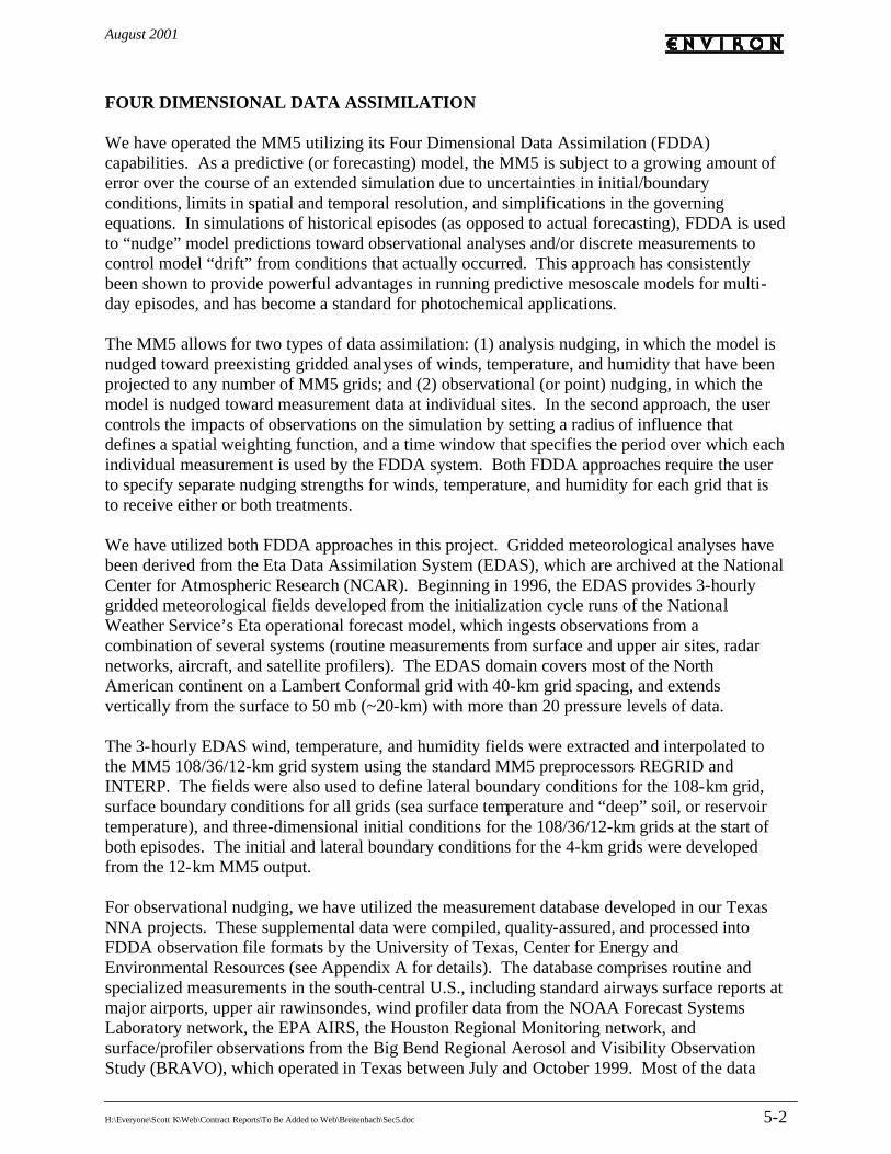
August 2001


FOUR DIMENSIONAL DATA ASSIMILATION We have operated the MM5 utilizing its Four Dimensional Data Assimilation (FDDA) capabilities. As a predictive (or forecasting) model, the MM5 is subject to a growing amount of error over the course of an extended simulation due to uncertainties in initial/boundary conditions, limits in spatial and temporal resolution, and simplifications in the governing equations. In simulations of historical episodes (as opposed to actual forecasting), FDDA is used to “nudge” model predictions toward observational analyses and/or discrete measurements to control model “drift” from conditions that actually occurred. This approach has consistently been shown to provide powerful advantages in running predictive mesoscale models for multi-day episodes, and has become a standard for photochemical applications. The MM5 allows for two types of data assimilation: (1) analysis nudging, in which the model is nudged toward preexisting gridded analyses of winds, temperature, and humidity that have been projected to any number of MM5 grids; and (2) observational (or point) nudging, in which the model is nudged toward measurement data at individual sites. In the second approach, the user controls the impacts of observations on the simulation by setting a radius of influence that defines a spatial weighting function, and a time window that specifies the period over which each individual measurement is used by the FDDA system. Both FDDA approaches require the user to specify separate nudging strengths for winds, temperature, and humidity for each grid that is to receive either or both treatments. We have utilized both FDDA approaches in this project. Gridded meteorological analyses have been derived from the Eta Data Assimilation System (EDAS), which are archived at the National Center for Atmospheric Research (NCAR). Beginning in 1996, the EDAS provides 3-hourly gridded meteorological fields developed from the initialization cycle runs of the National Weather Service’s Eta operational forecast model, which ingests observations from a combination of several systems (routine measurements from surface and upper air sites, radar networks, aircraft, and satellite profilers). The EDAS domain covers most of the North American continent on a Lambert Conformal grid with 40-km grid spacing, and extends vertically from the surface to 50 mb (~20-km) with more than 20 pressure levels of data. The 3-hourly EDAS wind, temperature, and humidity fields were extracted and interpolated to the MM5 108/36/12-km grid system using the standard MM5 preprocessors REGRID and INTERP. The fields were also used to define lateral boundary conditions for the 108-km grid, surface boundary conditions for all grids (sea surface temperature and “deep” soil, or reservoir temperature), and three-dimensional initial conditions for the 108/36/12-km grids at the start of both episodes. The initial and lateral boundary conditions for the 4-km grids were developed from the 12-km MM5 output. For observational nudging, we have utilized the measurement database developed in our Texas NNA projects. These supplemental data were compiled, quality-assured, and processed into FDDA observation file formats by the University of Texas, Center for Energy and Environmental Resources (see Appendix A for details). The database comprises routine and specialized measurements in the south-central U.S., including standard airways surface reports at major airports, upper air rawinsondes, wind profiler data from the NOAA Forecast Systems Laboratory network, the EPA AIRS, the Houston Regional Monitoring network, and surface/profiler observations from the Big Bend Regional Aerosol and Visibility Observation Study (BRAVO), which operated in Texas between July and October 1999. Most of the data

August 2001


were recorded hourly, except the 12-hourly standard NWS rawinsondes. The resulting FDDA input files were used to nudge the MM5 on the 12 and 4-km grids for both modeling episodes. MM5 CONFIGURATION The MM5 provides a wealth of options to configure the model for various parameterizations and physics packages. We have configured the model based upon the MM5 simulations performed for the NNA applications. We have determined that these are the most appropriate options for each nested grid and for the meteorological conditions existing in the area of concern. Selection of these options has been guided by Dr. Nelson Seaman of Pennsylvania State University (PSU). A few matters of concern that were identified at the start of this and the NNA modeling projects included the convective rainfall activity in northern Texas and Oklahoma during much of the September 1999 episode, and the onshore propagation of a hurricane into southern Texas during the August 1999 episode. We have seen that thunderstorm development in MM5, particularly on the finest grids (4-km grid spacing) can lead to performance problems with wind speeds/directions, near-surface temperatures, and boundary layer depth. This is related to the stochastic nature of these events, where MM5 qualitatively performs well in placing convective activity in the correct area during the appropriate time of day, but quantitatively cannot reproduce the strength, location, and timing of individual thunderstorm cells. An initial MM5 run (labeled herein as “Run 1”) was made for both episodes that invoked the analysis nudging capabilities of the model, and that was configured with the physical treatments and options that in our experience have worked best in past photochemical modeling exercises. This configuration included: • Two-way interactive 108/36/12-km grids, and two independent one-way interactive 4-km

grids located over DFW and the south-central Texas area (depending on episode, see Section 3).

• FDDA analysis nudging on the 108/36/12-km grids: - Above about 1500 m to model top: MM5 was nudged toward 3-hour EDAS analyses of

winds, temperatures, and humidity; - In the boundary layer: we relied on the latest MM5 boundary layer scheme to define the

distribution of winds, temperature, and moisture up to 1-3-km above the surface for all grids so that the relatively coarse (time and space) EDAS analyses would not influence the development of mesoscale boundary layer processes.

• The Gayno-Seaman boundary layer turbulence scheme was employed for all grids. • Simple-ice cloud microphysics was employed for all grids. • The Kain-Fritsch cumulus parameterization, which accounts for the effects of sub-grid scale

convective activity, was invoked for all grids except the 4-km nests (no cumulus parameterization was invoked for the 4-km grid as convection should be fully resolved at this scale).

• The simple single-slab “force-restore” soil model was used to model surface temperature (the user is limited to only this choice for certain selections of boundary layer scheme, including Gayno-Seaman).

• The cloud radiation scheme, which accounts for solar and terrestrial radiation impacts due to the presence of clouds, was used for all grids.

August 2001


The purpose of this initial run was to establish a baseline simulation that could be considered a “hands-off” application, configured in a typical or “standard” manner for photochemical applications. We have invoked the new boundary layer scheme now available in MM5 version 3, but elected not to utilize the (as yet) largely untested Land Surface Model (LSM) component. The analysis nudging was applied with standard grid-dependent nudging strengths as suggested by NCAR and PSU to control model drift on the larger synoptic-scale grids over the course of the long integration period. Thus, this first run provides clues about basic MM5 performance free of any further user intervention aimed at maximizing performance for these episodes. An additional “Base Case” run (labeled herein as “Run 2”) was then undertaken that is identical to the first, but adds the following component: • FDDA observational nudging of winds on the 12 and 4-km grids from routine and special

measurement data available in Texas during the episode (see Appendix A): - At the surface: MM5 was nudged toward observed winds only; - Aloft: MM5 was nudged toward 12-hourly rawinsonde and hourly profiler wind data both

in the boundary layer and in the free troposphere. We have chosen not to nudge temperature or humidity. The vast majority of observation data are at the surface, and it is widely known among meteorological modelers that nudging toward near-surface temperature observations can lead to unrealistic responses in the model, and therefore dire consequences in the dynamic fields. Nudging humidity is generally less of a problem, but for similar reasons of thermodynamic balance, we leave the MM5 to fully simulate the water vapor cycle on its own in the boundary layer. Several user-defined variables must be set that describe the strength of nudging and the spatial/temporal influence of each observation on the simulation. The strength is given by the “nudging coefficient”, which can be viewed as a relaxation time scale. For the Base Case run, we chose a standard value of 4×10-4 s-1 for both the 12 and 4-km grids, as suggested by NCAR and PSU. The spatial influence of each observation is specified by the “radius of influence.” A grid cell within one or more radii is influenced by those observations, weighted by the relative distance to each observation site. For the Base Case run, we chose a 10-cell radius of influence, meaning that a value of 120 km was chosen for observational nudging on the 12-km grid, and 40 km was chosen for the 4-km grid. The temporal influence of each observation is specified by the “time window”, which is the half-period over which an observation will be used for nudging. A temporal weight of 1 is used within this window, and this weight ramps down to zero over an additional period of the same length before and after the observation time. For the Base Case run, we chose a 40-minute time window, which means that MM5 will nudge toward this observation at full strength 40 minutes before and after the observation time. This value was suggested by NCAR and PSU. Other nudging parameters were selected based on past experience: (1) the frequency to calculate nudging coefficients (in coarse grid time steps) was set to 1 (every step); and (2) the vertical radius of influence (in sigma units) was set to 0.001, which means that we are not allowing an observation to influence layers above or below the respective measurement height. QUALITATIVE ASSESSMENT OF RESULTS

August 2001


A qualitative assessment of surface and aloft wind, temperature, pressure, and precipitation patterns in the initial simulation (Run 1) has been undertaken for each episode. The evaluation was based upon a comparison between various graphics of simulated and observed fields. A full writeup of the results are provided in Appendix B and C. Here, we summarize the results of the assessment for each episode day (neglecting the first 2 spinup days) and provide example figures. A companion CD to this report contains all of the MM5 graphics for winds, pressure, temperature, and precipitation plotted at 12-hourly intervals, as well as observational surface maps obtained from Unisys (http://weather.unisys.com/archive/index.html). Following the discussion for each episode, we provide a brief description of MM5 performance in replicating 12-hourly upper air profiles of temperature, humidity, and wind speed/direction at Dallas Fort Worth (August episode), and at Lake Charles (September episode). The MM5 Run 2 (with observation nudging of winds) is plotted against the observations to evaluate how well the full FDDA case performs in the vertical at these key sites. Emphasis is placed on performance in the lowest 2-3 km, and again only the episode days are analyzed. The sounding plots for both episodes are provided in Appendix D. August 1999 Episode August 15 At 0600 CST, the MM5 properly replicated the major synoptic features in the Midwest, and their propagation eastward. This included a surface trough from Nebraska to New Mexico, and a high pressure system over Ohio. A tail end of a week cold front extended into Louisiana and eastern Texas. At 500 mb, the model did a good job replicating the upper level high pressure dome centered over Oklahoma. In northern Texas, sea-level pressure continued to be simulated high since the beginning of the simulation. This likely caused an incorrect simulation of offshore flow over the southern Texas coastline. In the Dallas domain, the simulated winds matched the observations (5 knots, east-southeasterly). Results were mixed for temperatures; Shreveport was 5 F too warm while Dallas was 3 F too cool. At 1800 CST, MM5 correctly predicted a NE-SW oriented surface trough through Nebraska. Pressure remained too high over northern Texas, which possibly caused the tail of the coastal front to drift into the Gulf instead of staying onshore (Figure 5-1). MM5 simulated the sea breeze in Texas, but it was not as strong as observed. The northerly wind component was a little strong over the eastern portion of the state (northeast simulated vs. east-northeast observed). In Dallas, the east-southeast winds were 5 knots rather than the 10 knots observed. Temperatures tended to be too low by 5-8 F. The precipitation fields in southern and central Texas were well simulated. August 16 At 0600 CST, MM5 replicated all the major observed synoptic features, and simulated the upper level pressure heights and winds beautifully. The main problem continued to be the over predicted high pressure in Texas. This led to stronger pressure gradients in eastern Texas and Louisiana, and higher predicted northeasterly winds (5 knots) than observed (calm). However, in Dallas the 5 knot southeasterlies fit well with observations. Early morning temperatures were simulated reasonably well over inland Texas, but were too warm near the coast (lower 70’s

August 2001


predicted vs. lower 60’s observed). At 1800 CST, MM5 correctly simulated wind convergence along a frontal zone in Kansas, but continued to have problems with pressure in northern Texas. The over prediction of 2 mb, while better than on previous days, dampened the simulated wind speeds across the state. Wind convergence over the Texas Panhandle was over predicted, leading to convective precipitation and lower temperatures in that area (lower 80’s vs. mid- to upper-90’s observed). Temperatures were also too cool along the coast. While MM5 correctly predicted an afternoon sea breeze along the entire Texas and Louisiana coastlines, the strength and inland penetration was much too weak as the flow around the high pressure to the north blocked its development (Figure 5-2). In Dallas, the wind speed was weaker than observed (5 knots vs. 10 knots) and the direction differed by about 30 degrees. Temperature in that area remained about 5 F too cool. August 17 At 0600 CST, MM5 simulated the frontal boundary over central Kansas well. Simulated pressure rose over the southeast U.S., concurring with observations. MM5 also correctly positioned the center of high pressure over Oklahoma, and matched the radar echoes with precipitation across much of the Texas coast. Temperatures were simulated about 10 F too high in northern Texas, and 5 F too warm near the coast. In East Texas, 5 knot easterly winds were simulated while Shreveport reported calm. MM5 did a much better job in Dallas, where the 5 knot southeasterly winds and temperatures in the low 70’s matched observations. At 1800 CST, MM5 replicated wind patterns and precipitation along the surface trough and warm front in Kansas (although rainfall did not appear as widespread as observed). Precipitation also matched radar echoes in Texas and central Louisiana as the sea breeze penetrated inland and created a convergence zone. Thus, the strength of the sea breeze appeared correct (Figure 5-3). The 5 knot northeast winds in Shreveport matched observations well. Also, the 5-10 knot east-southeast wind in Dallas was fairly close to the measurements. Temperatures, however, were under predicted in Dallas (lower 90’s vs. upper 90’s). August 18 At 0600 CST, MM5 seemed to predict a surface low pressure system over northeast Kansas reasonably well. Aloft, MM5 simulated the upper level high perfectly. On the coast, MM5 did a fine job over Louisiana, but simulated offshore winds at 5 knots in Texas when most coastal sites reported calm. Once again, pressure up to 4 mb too high over Texas’ interior may have triggered this problem. In northern Texas, observations were all southerly at 5 knots; while MM5 captured these features in northwestern Texas, there were problems in the northeast. Simulated winds in Dallas were southeasterly instead of southerly, and in East Texas, northwest winds were simulated. Morning temperatures were over predicted near the coast and inland (80 F predicted vs. mid-70’s observed). At 1800 CST, MM5 replicated the position of the frontal boundary moving into the Texas Panhandle quite well. Modeled precipitation over Louisiana was pushed farther inland than observed, and precipitation over central Texas was erroneous. The simulated sea breeze was stronger than observed (similar to Figure 5-3), creating more inland convergence and precipitation. However, MM5 correctly weakened the sea breeze relative to the previous day. Pressure over inland Texas remained a few millibars too high, but the pressure gradient over the state was minimal, as observed. The light and variables winds were well represented in Dallas,

August 2001


as were the light northeast winds in Shreveport. Daytime temperatures were 3-5 F below observed in Texas, and were particularly low (nearly 10 F) near the coast due to the over predicted sea breeze. August 19 At 0600 CST, MM5 replicated features at 500 mb very well, including the westward propagation of a 500 mb high over New Mexico, and a new trough digging into the midwest. The model also maintained the same sea level pressure problem in Texas. Wind convergence near the Oklahoma-Texas border suggested a correct location of the observed frontal system. Ahead of this front, calm to 5 knot winds agreed with observations. Winds overall were rather light. In Shreveport, the west-northwesterly simulated winds should have been southwesterly. In Dallas, a convergence line seemed to have formed (westerly to the south, easterlies/southerlies to the north), but no precipitation was associated with it. Again, morning temperatures were too warm (70’s to mid 80’s vs. 60’s and 70’s observed). At 1800 CST, the most notable feature was the simulation of a surface trough over central Texas and southern Louisiana instead of over the northern portions of these states. MM5 predicted a sea breeze that did not penetrate as far inland as the previous day, yet observations suggested stronger onshore winds and greater inland penetration. As a result, the simulated wind convergence boundary was predicted closer to the coast. Again, surface pressure was about 2-3 mb too high in the western part of Texas. In Dallas, predicted winds were light and variable as a mesoscale low formed over the area; observations were southerly. The surface trough should have cut across this domain and created precipitation over Dallas. In East Texas, MM5 properly simulated 5 knot northwesterlies, with some weak variability. Coastal temperatures were too low along the southern Texas coast, but were reasonable near Houston and Lake Charles. The interior was difficult to evaluate due to the precipitation there. Shreveport temperature was under predicted (94 F vs. 100 F). August 20 At 0600 CST, MM5 properly simulated a trough propagating southward into Georgia, and the stationary high pressure over New Mexico. It also replicated the wind field over Texas very well. The convergence zone along the frontal boundary extending into Texas matched beautifully, with northerly winds behind the front and lighter northwesterly winds ahead. In Dallas, the northerly direction matched observations well, but the speed was weaker by 5 knots. Very good performance was seen in East Texas, where winds were predominantly northeasterly at 5-10 knots. The pressure field continued to be higher than observed over western Texas, yet the inland temperatures were quite close. Coastal temperatures were too warm. At 1800 CST, the frontal boundary hovering in the Gulf states was simulated as evidenced by the wind convergence patterns, but MM5 placed it too far north. The model generated a 10 knot southerly wind over Houston feeding into the front to the north, but the front should have been south of Houston, where a northerly wind was measured (Figure 5-4). Along the Texas southern coastline, the sea breeze penetrated a little too far inland, and the onshore direction was about 45 degrees off. Interior pressure remained too high over northern Texas, which weakened the flow in this region. In the East Texas domain, MM5 predicted a northeast 5 knot wind that differed from the Shreveport observation by 30 degrees (north-northeast). The model remained about 5 F too cool in many locations (including focus cities in the north), but it was worse in Houston due to the incorrect position of the frontal boundary and precipitation.

August 2001


August 21 At 0600 CST, the 500 mb high continued to be predicted well. At the surface, pressure remained too high in northern Texas, causing the flow around the high to be distorted from observations in the focus areas (northeasterly simulated vs. easterly observed). In Dallas, however, the 5 knot east-northeasterly wind matched the observations. Coastal Texas winds exhibited some problems; Houston reported a 5 knot onshore wind heading toward the stalled front just to the north, while MM5 simulated a light offshore flow. Corpus Christi reported calm conditions, but MM5 simulated a 5-10 knot north wind. Temperatures did not cool down sufficiently over night, as lower 80’s were predicted and upper 70’s were observed. The model performed better in the interior 4-km domains, with lower 70’s predicted within 2 degrees of observations. At 1800 CST, pressure over northern Texas remained a big problem (by 2-3 mb). Again, this led to a distorted high and stronger northerly wind components in eastern Texas. MM5 developed a northeast wind over Shreveport when observations were east-southeasterly. In Dallas, winds were primarily easterly instead of southeasterly. Winds along the coast looked reasonable, with convergence simulated along the stalled frontal boundary (similar to Figure 5-4). The MM5 sea breeze did not seem to penetrate as far inland as observed. MM5 continued to be conservative with temperatures over Texas. The highest predicted temperature was 93 F, but numerous observations were in the upper 90’s. The model performed well in simulating the precipitation field and matched the location of radar echoes. August 22 At 0600 CST, MM5 matched the position of a low pressure center and associated trough in Oklahoma. The upper level features were again well simulated. Pressure in northern Texas was again up to 3 mb too high, creating a stronger pressure gradient and stronger southerly wind in northern Texas. However, the wind fields in the East Texas domain seemed immune to this pressure problem as the 5 knot east-northeast winds matched observations. The winds in Dallas also matched the observed 5 knot east-southeasterlies. The model did a good job simulating the location and strength of the hurricane entering extreme southern Texas. Simulated morning temperatures were too warm. For example, Shreveport measured 70 F, but predictions were in the upper 70’s. At 1800 CST, the persistent over prediction in pressure spread into central Texas (1013 mb near San Antonio vs. 1009 mb observed). Pressure was also too high along a surface trough through the Texas Panhandle. Yet the wind field resembled the observed patterns rather well: MM5 simulated a 10 knot southerly wind over northern Texas, easterly onshore flow that penetrated well into Texas’ interior, and gusty winds in southern Texas near the hurricane. The model did a good job predicting a northeast 5 knot wind over Shreveport. In Dallas, the 10 knot southeasterlies were about 30 degrees off from observed directions (Figure 5-5). Comparison of Run 2 to Sounding Data at Dallas-Fort Worth Inspection of the observed and MM5 Run 2 sounding data at DFW (Appendix D) revealed that the MM5 performed rather well for winds, but that the boundary layer was generally too cool by a few degrees, and that moisture was over predicted, sometimes by as much as a factor of two. The cool boundary layer tended to result in low boundary layer heights (as diagnosed from

August 2001


humidity and temperature profiles) on three out of the eight episode days: • August 17: 1 km predicted versus 2 km observed • August 18: 2 km predicted versus 3 km observed • August 19: 1.5 km predicted versus 2.5 km observed

The periods in which wind speed performance was poor included the following: • August 16, 1800 CST: 4 m/s predicted versus 6 m/s observed • August 18, 1800 CST: 4 m/s predicted versus near calm observed near the surface • August 19, 0600 CST: 0-2 m/s predicted versus 2-6 m/s observed • August 19, 1800 CST: 4-6 m/s predicted versus 2-4 m/s observed • August 22, 0600 CST: 2-5 m/s predicted versus 5-9 m/s observed

The days in which wind direction performance was poor (>30 degrees difference) included the following: • August 18, 1800 CST: ~60 degree difference • August 19, 1800 CST: ~90 degree difference • August 22, 0600 CST: ~60 degree difference September 1999 Episode September 15 At 0600 CST, MM5 correctly simulated the tightening of the surface pressure gradient over the southeast U.S. as high pressure over the upper Midwest expanded in size and Hurricane Floyd moved up the Gulf Stream toward south Carolina. However, the pressure gradient was simulated to be too tight over southeastern Texas, as pressure over central Texas was too high. As a result, the predicted wind speed along the Texas coast was 10 knots instead of calm to very light as reported (although overall the simulated direction was correct). In northern Texas, MM5 over predicted the northerly wind component as a result of flow around the ridge axis. Aloft, MM5 simulated a trough over the Plains rather well, along with associated weakening winds. Morning temperatures were well replicated. Winds in San Antonio (5 knot northeasterly) fit the observation well. Near the coast, MM5 over predicted wind speed as 10 knot northerly winds should have been 5 knots or less. The simulated precipitation east of Corpus Christi agreed with observed radar echoes. At 1800 CST, MM5 over predicted the strength of high pressure over the northern Plains somewhat and placed it more to the east; in Texas, pressure in the middle of the state continued to be about 2-3 mb too high, causing flow near San Antonio to be east-northeast instead of east-southeast. In addition, the stronger pressure gradient near the Texas coast resulted in a 10 knot northeast wind over Corpus Christi when a 5 knot southeast onshore wind was observed. The model performed well in Houston, where no sea breeze was predicted (Figure 5-6). Daytime temperatures appeared to be a little too low over states bordering the Gulf. Texas coastal areas were under predicted, and this extended to San Antonio (80 F predicted vs. 90 F observed). Inland, MM5 performed better and correctly showed a significant drop into the upper 50’s in the Texas Panhandle. The model correctly kept the coastal regions dry, but failed to replicate the

August 2001


radar echoes over northern and central Texas. September 16 At 0600 CST, the pressure field simulated by MM5 resembled the analyzed field very well, except for the persistent trouble in central Texas. This caused the wind along the Texas coast to be a bit too strong. Direction appeared reasonable, for the most part, although there was a 45 degree disagreement over San Antonio and Dallas. MM5 predicted temperatures well, ranging from the upper 50’s in the Texas Panhandle to the 70’s along the immediate coast (although Houston was a little too warm). Winds in the 4-km domain were predominately north-northeasterly at 5 knots in the interior, and up to 10 knots by the coast. This looked reasonable near Corpus Christi, but was too fast near Houston (observed calm). In the interior, MM5 was unsuccessful in directing winds near San Antonio to a northwesterly direction. No precipitation was observed nor predicted in the region. At 1800 CST, MM5 positioned a high pressure system over the northern Plains too far east. This affected wind direction in northwestern Texas (southeasterly predicted vs. easterly observed). Unlike other periods, the pressure field over Texas seemed more reasonable. The temperature gradient across Texas was too weak (upper 60’s in the Texas Panhandle to mid 80’s in the south); the coastal stations were all under predicted by about 5 F. Once again, MM5 simulated very little precipitation but there were radar echoes near Dallas. The sea breeze was stronger and influenced a greater area compared to the previous day, agreeing with observations. Winds in San Antonio should have had a more southerly component. MM5 correctly simulated a 10 knot onshore east wind over Corpus Christi, but also lacked a weak southerly component. Toward Victoria, onshore flow weakened, and was completely gone in Houston where the model correctly simulated a 5 knot northeast wind (Figure 5-7). September 17 At 0600 CST, MM5 seemed to develop the surface high over the upper midwest too strongly, which induced pressure to be too high over central Texas once again. MM5 performance aloft looked good, and the model replicated the upper level winds well where they were strong; however, where the upper winds were week (New Orleans and Corpus Christi), the simulated direction was not correct. Temperatures were simulated well except on the immediate coast where they were too warm. Precipitation was also simulated well since most of Texas was dry. The winds in the 4-km grid were northeasterly at 5 knots in the interior, and MM5 simulated a small area of calm winds close to San Antonio and Austin, as observed. Near the coast, the wind direction near Houston should have been northerly instead of northeasterly, while winds in Corpus Christi were well simulated. At 1800 CST, MM5 did not simulate the high pressure over the Great Lakes very well. This problem may have also enhanced the pressure problem over central Texas (1018 mb simulated vs. 1014 mb observed). Temperatures were about 5 F too low over most areas of Texas. In the 4-km domain, the afternoon sea breeze looked very similar to the previous day: winds in Corpus Christi were simulated at 10 knots, but lacked a slight southerly component, and winds in Houston remained parallel to the coastline at 5 knots. In San Antonio, 5 knot southeast winds matched observations, and a 5 knot east-northeast wind was simulated over Austin. Some precipitation was generated west of Corpus Christi due to a convergence of the sea breeze and a microscale high. However, no radar echoes were observed anywhere in the 4-km domain.

August 2001


September 18 At 0600 CST, MM5 continued to have problems with the pressure field. It simulated a fictitious inverted ridge axis that extended into Texas. At 500 mb, MM5 looked reasonable with a few short waves west of the Texas Phanadle, agreeing with observations. Early morning temperatures were simulated quite well, with 60’s across most of Texas. The model correctly kept Texas dry during the hour, except for a few light areas near Corpus Christi (not observed). The 4-km domain was rather quiet inland. Offshore flow was simulated over the northern Texas coast (Houston was reported calm), while winds were along the shoreline in the south (a good fit in Corpus Christi). Inland, wind speeds at 5 knots or less were well simulated in San Antonio (calm). At 1800 CST, MM5 forecast sea level pressure up to 4 mb too high with the erroneous inverted ridge. Otherwise, the model correctly predicted lower pressure moving into Nebraska and in the Gulf. Temperatures were predicted fairly well over Texas with 70’s near the Panhandle to the 80’s in the rest of the state. The midsection was slightly under predicted by about 4 F. Light precipitation was well simulated in the areas of radar echoes. The observed sea breeze was much stronger compared to the previous day, but MM5 seemed to make it weaker (similar to Figure 5-7). A southeast wind should have penetrated to San Antonio; MM5 simulated flow did not penetrate inland beyond Corpus Christi or Victoria. Although the model did simulate southeast winds near San Antonio, a large area of

August 2001


northeasterly winds separated the area from the coast. In addition, the model failed to simulate a sea breeze in Houston, where the southeasterly breeze could not overcome the large scale northeasterly flow. September 19 At 0600 CST, MM5 persisted with the same problems; high pressure extended too far to the southwest from the Ohio Valley affecting the middle of Texas. A tropical storm over the Gulf south of Louisiana was well replicated. Aloft, MM5 predicted a weak trough between Nebraska and eastern Texas, agreeing with observations. Early morning temperatures were well replicated, except along the immediate coast where MM5 was too warm. The 4-km grid was relatively quiet with no precipitation. Winds were northerly at 5 knots near the coast and light and variable in the San Antonio and Austin areas. Observations were all at 5 knots or less. In Houston, MM5 predicted winds a little too fast, while predictions agreed well in Corpus Christi. At 1800 CST, the MM5 simulation looked very good. The model correctly replicated the position of a surface trough heading eastward over northern Texas, although the model was about 2 mb too high. A very tight temperature gradient was well replicated, with 60’s in the extreme north to lower 90’s in central Texas. Coastal temperatures were also in agreement with observations in the 80’s. Onshore flow was simulated in the 4-km domain from south of Houston to the Brownsville. MM5 correctly simulated no sea breeze over Houston, which indicated a northeast wind. The model continued to lack the southerly wind component over Corpus Christi (easterly simulated vs. southeasterly observed). Had the direction been correct, Gulf air could have flowed directly into San Antonio, where a south-southeast wind was correctly simulated (Figure 5-8). Austin was too far inland to be affected by the southeast flow. September 20 At 0600 CST, MM5 correctly predicted a vast area of 10 knot winds and strong high pressure building behind a front propagating through Oklahoma and northern Texas. However, the tail end of the front did not move through Texas as quickly as analyzed. This may be related to the erroneously higher pressure over the state, slowing the propagation of the front. MM5 maintained the position of the tropical storm in almost the same location in the Gulf rather than moving it eastward. MM5 correctly replicated the major features aloft. Early morning temperatures did not drop enough in the simulation, with upper 50’s in the Panhandle (lower 50’s observed) to the mid-70’s near the coast (mid-60’s observed). In the 4-km domain, MM5 correctly simulated offshore flow along the Texas coast. Winds in Corpus Christi fit observations well, and the winds in Houston were northerly. Inland, both San Antonio and Austin were calm as MM5 under predicted the wind speed. At 1800 CST, the MM5 simulated the large scale features well. However, the simulated front lagged the observed front over Texas and Arkansas. As a result, slower winds were simulated over northeast Texas. Temperatures looked good with a strong gradient behind the cold front. MM5 performed well in predicting 50’s in the Panhandle to 90 F in the center of the state (a slight under prediction). Precipitation was also well replicated with rainfall near Dallas. Radar echoes near San Antonio were not simulated. In the 4-km domain, the sea breeze was suppressed close to the shoreline over the northern coast (agreeing with observations), but the breeze was too weak over the south coast. Houston’s north wind differed by about 45 degrees from observations. Farther south, easterly 5 knot winds in Corpus Christi should have been southeasterly at 10 knots. Simulated pressure was almost 3 mb greater than observed in interior,

August 2001


hindering the inland penetration of the sea breeze. Comparison of Run 2 to Sounding Data at Lake Charles While wind performance was promising at Lake Charles, MM5 Run 2 did not perform as well during this episode as it did in the August episode at DFW. This was likely due to the site’s location near the Louisiana coastline, and subject to the ability of MM5 to adequately simulate the sea breeze circulation. The boundary layer wind speeds were generally over predicted on most days by factors ranging from 1.5 to 4. Wind direction was well simulated, however, with only three periods (August 18, 1800 CST; and August 20, 0600 and 1800 CST) indicating directional error through the boundary layer of about 60 degrees. Again, the boundary layer was generally too cool by a few degrees, and moisture was over predicted. Boundary layer heights were well predicted on only a couple of days. On most days, MM5 predicted a boundary layer depth of 1-1.5 km while the observed humidity/temperature profiles suggested an actual boundary layer depth of 2-2.5 km. STATISTICAL EVALUATION A quantitative assessment of MM5 performance in replicating surface-level wind, temperature, and humidity measurements was undertaken by calculating the statistical parameters discussed in Section 4. Statistics were calculated for both hourly and daily time scales, and for various portions of the modeling grid, including: (1) the entire 12-km grid for both episodes (typically 133 sites); (2) the HG/BPA 4-km sub-domain for the September 1999 episode (typically 35 sites); and (3) the DFW 4-km grid for the August 1999 episode (typically 18 sites). The site locations within each of these domains are shown in Figures 5-9 through 5-11. Performance is discussed relative to the proposed statistical benchmarks developed in Section 4. August 1999 Episode Results on the 12-km Regional Grid Hourly Statistics Hourly statistical results for Run 1 on the 12-km grid are presented graphically in Figure 5-12 for winds, temperature, and humidity. Mean and error statistics are generated from a sample of about 130 sites each hour. Starting with surface winds (Figure 5-12a), the light wind conditions during the episode are replicated overall, with the mean observed and predicted speeds remaining below 4 m/s over the entire period. However, the most obvious performance issue is the very regular pattern of over predicted wind speeds during nighttime hours, and the under predictions during the daytime. This is most clearly seen in the hourly bias. The RMSE for wind speed also indicates a diurnal error pattern, and suggests that the bulk of RMSE is comprised of the systematic component. This indicates that a systematic error is occurring that might be reduced with a relatively simple refinement to the model or it’s inputs. The unsystematic component is much lower, remaining around 1 m/s throughout the episode. The IOA for wind speed varies around 0.6, which is considered to be quite good. The wind direction is well replicated on an hourly basis over the 12-km domain, with bias typically well within 30 degrees and peak bias in any single hour not exceeding 50 degrees.

August 2001


The regular nocturnal over prediction in wind speed has been seen in other MM5 applications in the past, most notably in the midwestern U.S. However, its coupling to a significant under prediction during the day is a cause for concern. It is as if the entire diurnal tidal forcing is half a wavelength out of phase. The reasons for the nocturnal over predictions remain unclear, however we have developed some hypotheses to explain the problem. The most likely cause may stem from the improper development or over-excitation of the low-level jet, a well-known and often observed nocturnal phenomenon throughout the midwest that develops from boundary layer forcings within 1 km of the surface. In any event, it is likely that too much momentum is being transferred to the surface from just above via mixing. As for the daytime under predictions, it is likely that the over predicted surface pressure in Texas is flattening the pressure gradient regionally, as described earlier in the qualitative assessment, and leading to excessively weak winds. The hourly mean temperature pattern (Figure 5-12b) shows a nice agreement with observations, and follows the day-to-day variation fairly well. Temperature RMSE ranges from 1.5 to 3 K, with some higher peaks; as for wind speed, the bulk of the RMSE lies in systematic error as the unsystematic error ranges between 1 to 1.5 K. The IOA is generally quite good, with a few notable exceptions. Note that the daily maximum temperatures appear to be under predicted by a few degrees, while the daily minimum temperatures appear to be over predicted by a similar amount. One cause for this is related to the vertical resolution in MM5. The lowest layer midpoint (half-sigma level) is at about 10 m. While this agrees well with most wind measurements taken from 10 m masts, “surface” temperature is usually recorded within 1-3 m of the ground. During the daytime, the temperature at 10 m is cooler by several degrees, and at night the temperature at 10 m can be warmer. Tests were conducted with this database in which temperatures from the lowest two MM5 layers were linearly extrapolated to the ground. This significantly reduced the peak daytime error, but did little for the minimum temperature each morning because the MM5 often generates an isothermal temperature structure at night (rather than an inversion). Similar tests have been conducted by other investigators (e.g., Bornstein, personal communication), in which extrapolations are more appropriately based on log-profiles defined by micro-meteorological parameters output by MM5. In these cases, errors in daily maximum and minimum temperatures were almost entirely removed. Therefore, under predictions of daily maximum temperatures shown here are not necessarily a cause for concern as long as they are within 1-2 degrees. However, we remain cautious regarding the over predictions of daily temperature minima, and the related fact that MM5 tends not to stabilize the surface layer at night as observed. Furthermore, this is most certainly interrelated with the high nocturnal winds, which are mixing down to the surface too easily, and/or are causing too much mechanical turbulence that prohibits a cooling of the surface and proper stabilization of the surface layer. Predicted humidity (Figure 5-12c) follows the observed trend throughout the episode. However, it is consistently over predicted by about 1-2 g/kg. The RMSE averages 3-4 g/kg during the period, with most error associated with the systematic component. The IOA is on par with the temperature performance.

August 2001


One hypothesis explaining the consistent over prediction of humidity is that soil surface is too moist by default. This would provide a consistent source of moisture to the boundary layer, and also tend to dampen the diurnal temperature wave (as seen in Figure 5-12b) since more heat energy is transferred to latent heat as moisture evaporates from the soil. An overly wet soil might explain the performance for temperature, the lack of nocturnal stabilization, and possibly even the abundant mixing of winds to the surface. This issue is investigated further in sensitivity runs described in Section 6. Hourly statistical results from the Run 2 Base Case (observational nudging of winds on the 12- and 4-km grids) are not significantly different from the results of Run 1. In the interest of brevity, the hourly plots for Run 2 are not shown. It is sufficient to mention that the performance for wind speed and direction were slightly improved on an hour-to-hour basis. Daily Statistics Daily statistical results for Run 1 on the 12-km grid are presented graphically in Figure 5-13 for winds, temperature, and humidity. Mean and error statistics are generated from a sample of between 3100 and 3200 hourly observations each day. The performance for surface winds is shown in Figure 5-13a; the trend for subsiding wind speed to August 18, and the subsequent increase is well replicated. The daily bias is well within 0.5 m/s; the daily gross error is at or below 1.5 m/s; and the RMSE is at or below 2 m/s (note that on this time scale, systematic and unsystematic errors are nearly equivalent). The IOA for wind speed ranges 0.5-0.6. Wind direction is quite well replicated over this domain, following the trend over the episode to start northeasterly, and rotate to easterly, then to southerly, then back to northeasterly toward the latter three days of the episode. Note that MM5 tends to lag this rotation by about 20 degrees. Wind direction bias is at or within 10 degrees (except on August 17), and the gross error is within 60 degrees. The daily performance for temperature is shown in Figure 5-13b. MM5 performs admirably in replicating the day-to-day trends throughout the episode. The cooling period (August 13-16) tends to be under predicted, while the warming period (August 17-20) tends to be over predicted. The daily bias remains at or within about 0.5 K, the gross error varies around 1.5 K, the RMSE is within 2.5 K, and the IOA ranges from 0.9 to 0.95. The daily performance for humidity is shown in Figure 5-13c. Again, the episode trends are faithfully replicated by MM5, but as seen in the hourly statistics, the humidity is consistently over predicted by 1 to 1.5 g/kg. Gross error and RMSE range from 2 to 3.5 g/kg, which is higher than desired. The IOA is lower than for temperature, ranging from 0.6 to 0.85. In order to more clearly see the impacts in performance for Run 2, Figure 5-14 displays the error statistics for Run 1 and Run 2 side-by-side. For winds (Figure 5-14a), the changes in bias and gross error are mixed and minimal over the entire 12-km domain. Interestingly, temperature and humidity appear to be more affected (Figures 5-14b and c), at least more than expected given that only wind observations were used for nudging. This indicates the intricate coupling between winds and surface fluxes of heat and moisture. A comparison of the daily statistics shown in Figure 5-14 for the Run 2 Base Case with the proposed benchmarks established in Section 4 is shown in the tabulation below. Those measures that exceed the benchmarks are shown in red. Note that we also report wind speed and direction bias to provide a more complete summary of wind performance.

August 2001


Parameter Benchmark Run 2 Range Run 2 Episode-Mean Wind Speed RMSE 2.0 1.7 2.0 1.9 Wind Speed Bias --- -0.4 0.6 0.1 Wind Speed IOA 0.6 0.44 0.67 0.55 Wind Direction Gross Error 20 32 57 42 Wind Direction Bias --- -14 10 -4 Temperature Bias ±0.5 -0.4 0.6 0.1 Temperature Gross Error 2.0 1.5 2.0 1.7 Temperature IOA 0.7 0.87 0.94 0.91 Humidity Bias ±1.0 0.2 1.8 1.0 Humidity Gross Error 2.0 1.8 2.8 2.3 Humidity IOA 0.7 0.59 0.85 0.73 Results on the DFW 4-km Grid Hourly Statistics Hourly statistical results for Run 1 on the 4-km grid are presented graphically in Figure 5-15 for winds, temperature, and humidity. Mean and error statistics are generated from a sample of about 18 sites each hour. Performance for wind speed (Figure 5-15a) is generally better than seen for the 12-km grid, with much smaller nightly over predictions. However, the daytime under predictions to near zero wind speed are equivalent or worse. The over predicted strength of the high pressure over central Texas described in the qualitative evaluation is surely the cause for this. The resulting pattern in speed bias again shows a consistent diurnal pattern between –2 and +2 m/s. The patterns for speed RMSE is similar to the 12-km grid results, varying around 2 m/s, but sometimes reaching as high as 4 m/s. The IOA is much lower, varying around 0.4. As expected with less prediction-observation pairings comprising these statistics, the performance for wind direction shows more variation over the course of the simulation, but is still quite good. Hourly bias error reaches up to and beyond 90 degrees for some hours. The performance for temperature (Figure 5-15b) is similar to the 12-km results. Overall, the day-to-day trend is captured well, and the daily minimum temperatures are very well replicated. However, the daily maximum temperatures are remain cool by a few degrees, and this trend holds for most of each day. This is shown by the consistent negative bias in temperature. Some odd over prediction periods occur, including a 3 K over prediction on the first day, and a consistently warm afternoon and evening on August 19. As seen in the wind direction plot, a significant directional error occurs on this day, which suggests that the timing and/or strength of frontal or trough activity through DFW may not have been accurate. The RMSE shows much larger variation than it’s 12-km counterpart (again, likely due to less data pairings), and peak RMSE values reach 4 K. IOA is quite low, with values varying around 0.4; it is particularly poor late on August 19. Hourly humidity performance (Figure 5-15c) is generally good, with the exception again on August 19 and 20. The observations and predictions seems to be out of phase on these days, which further suggests poor timing of the passage of a frontal boundary, and/or the consistent simulation of precipitation and clouds into August 20. With the introduction of observational nudging on the DFW 4-km grid in Run 2, hourly wind performance was slightly improved, particularly for direction for certain hours (including August

August 2001


19). Hourly temperature and humidity statistics were not significantly affected. Again, these plots are not shown. Daily Statistics Daily statistical results for Run 1 on the 4-km DFW grid are presented graphically in Figure 5-16 for winds, temperature, and humidity. Mean and error statistics are generated from a sample of about 430 hourly observations each day. The daily trend in wind speed (Figure 5-16a) is well replicated throughout the episode, with daily bias ranging from –0.7 to 1.1 m/s, and gross error at or below 1.5 m/s. Total RMSE remains below 2 m/s, but the IOA progressively deteriorates over the episode from about 0.6 to 0.2 on the last day. The trend in wind direction is well replicated for all days except on August 19, when the model maintains an easterly flow averaged over the day but the observations indicate northwesterly flow. Indeed, the daily gross error in direction on this day is in excess of 90 degrees, the maximum for the period. This directional error suggests that the MM5 was too slow in propagating a frontal trough through the DFW area on August 19. Daily temperature performance in the DFW subdomain (Figure 5-16b) does not appear to be particularly impressive, at least relative to the 12-km temperature results described thus far. A generally negative bias occurs during most of the episode, ranging from 1 to 2 K. However, the overall episode trends are replicated, with the warmest period being August 18-20. RMSE varies around 2 K as well, with a large systematic component. Note, however, that the unsystematic component maximizes on August 19, a day with nearly zero bias but typical gross error. This suggests a wide spread in measured temperature data for this day, a feature associated with stochastic details that MM5 may not be expected to replicate. Interestingly, the daily IOA remains quite high each day of the episode. This is in contrast to the hourly results (~0.4), which suggests that the IOA metric is sufficiently non-linear with the number of data pairings that one cannot infer a daily IOA value from a simple average of hourly IOA. Similarly to the hourly results, daily humidity (Figure 5-16c) is well replicated except on August 20, when the bias and gross error reach 4 g/kg, and RMSE reaches almost 5 g/kg. Typical bias and error range between 1 and 2 g/kg over the episode. The RMSE is comprised of a mix of systematic and unsystematic error, with the latter dominating on August 18 and 19. The IOA ranges from 0.36 (on the 19th) to 0.82. Figure 5-17 displays the daily statistical results for winds from Run 1 and Run 2 together. While the introduction of observation nudging in Run 2 has led to small mixed results for wind speed bias, a definite but small improvement is seen in gross error, RMSE, and IOA. The fact that these differences appear larger than for the 12-km grid results is likely due to the smaller number of data pairings. Like wind speed, the effect of observation nudging on directional bias is mixed, but the gross error is definitely improved (especially on August 19). Very slight improvements are seen for temperature in Run 2, but none are seen for humidity (plots not shown). A comparison of the daily statistics on the 4-km DFW grid for the Run 2 Base Case with the proposed benchmarks established in Section 4 is shown in the tabulation below. Those measures that exceed the benchmarks are shown in red.

August 2001


Parameter Benchmark Run 2 Range Run 2 Episode-Mean Wind Speed RMSE 2.0 1.3 2.1 1.6 Wind Speed Bias --- -1.0 0.9 -0.2 Wind Speed IOA 0.6 0.23 0.69 0.41 Wind Direction Gross Error 20 16 67 36 Wind Direction Bias --- -9 23 5 Temperature Bias ±0.5 -2.0 0.8 -0.9 Temperature Gross Error 2.0 1.4 2.1 1.7 Temperature IOA 0.7 0.87 0.95 0.92 Humidity Bias ±1.0 -0.9 4.1 0.9 Humidity Gross Error 2.0 1.4 4.5 2.0 Humidity IOA 0.7 0.36 0.83 0.53 September 1999 Episode Results on the 12-km Regional Grid Hourly Statistics Hourly statistical results for Run 1 on the 12-km grid are presented graphically in Figure 5-18 for winds, temperature, and humidity. Mean and error statistics are generated from a sample of about 130 sites each hour. The issues identified for wind speed in the August 1999 12-km results are seen again here (Figure 5-18a). Namely, there is a consistent diurnal bias wave, which is particularly prolonged during nighttime hours. However, the error remains within 2 m/s. The RMSE for wind speed is primarily comprised of the systematic component, and IOA appears quite good with variation around 0.7. Wind direction is replicated rather well through the entire episode, with some apparent deterioration near the end of the episode as frontal activity increases. A majority of hourly errors are within 10 degrees. The diurnal temperature wave, averaged over the 12-km grid (Figure 5-18b), displays similar patterns as seen for the August episode. The day-to-day trends are captured by the model, but daily maxima and minima are under and over predicted, respectively. Hourly errors tend to be biased low during the episode, reaching nearly 3 K, while the positive errors (early morning hours) are much less and of shorter duration. The RMSE for temperature ranges between 2-3 K, and is mainly composed of the systematic component, although the unsystematic component tends to dominant on the first two days. Hourly IOA is quite good, never dipping below 0.5, and reaching well over 0.9. Humidity is replicated rather well (Figure 5-18c), with a general trend of over predictions of less than 1 g/kg. For this parameters, the RMSE is more strongly influenced by the unsystematic component than seen for the August episode. The reason for this is unclear, but suggests that it might not be possible to substantially reduce total error in future sensitivity runs. Hourly IOA for humidity begins quite high, then lowers to a mean of about 0.7 later in the period. With the introduction of observational nudging of winds in Run 2, the hourly statistical performance for winds is only marginally improved (plot not shown). This is similar to the results seen for the August episode, and again is probably due to the large quantity of data pairings used in the hourly calculations.

August 2001


Daily Statistics Daily statistical results for Run 1 on the 12-km grid are presented graphically in Figure 5-19 for winds, temperature, and humidity. Mean and error statistics are generated from a sample of between 3100 and 3200 hourly observations each day. Winds remain light for the entire period, with a hint of a trend toward lower speeds to about September 19 (Figure 5-19a). MM5 replicates this trend, but tends to over predict on each day by about 0.5 m/s. Daily RMSE remains within 2 m/s, and indicates that the unsystematic component is higher late in the period. Daily IOA for wind speed varies around 0.5. Wind direction is very well replicated over the 12-km domain, following the slow trend in the observations from near northerly to easterly by September 19. The directional bias is quite near zero, while the gross error shows a slow tendency to grow toward the end of the episode. Most gross errors are within 45 degrees. The daily temperature tendency for this episode (Figure 5-19b) shows a minimum on September 16 and 17, and higher values at the beginning and end (unlike August, in which the key ozone days in the middle of the period are the warmest). While MM5 replicates the trend, it is over-amplified; the maxima are over predicted, and the minima are under predicted. The bias shows general under predictions on each day, up to 1 K. The gross error tends to be at or below 2 K. Daily RMSE ranges from 1.5 to 2.5 K, with roughly equivalent levels of systematic and unsystematic error. The IOA is quite good, ranging around 0.9 throughout the episode. The humidity trend follows the temperature trend, and MM5 replicates it well (Figure 5-19c). The tendency is for over predictions each day, by about 0.5-1 g/kg. Gross error varies about 1.5 g/kg, and the RMSE varies around 2 g/kg. Note that the unsystematic error dominates at the beginning of the episode, and that the two components are roughly equivalent for the remainder of the period. The IOA for humidity is quite good. The daily statistical results for Run 1 and Run 2 are compared in Figure 5-20. Unlike the August episode, a slight but definite improvement in wind speed is seen over the 12-km grid. Error numbers are reduced and IOA values are increased ever so slightly. While the directional bias appears mixed, the gross error does not change, or improves slightly toward the end of the period. Interestingly, bias and error measures for temperature are also improved slightly, while humidity numbers a more mixed (not shown). A comparison of the daily statistics shown in Figure 5-20 for the Run 2 Base Case with the proposed benchmarks established in Section 4 is shown in the tabulation below. Those measures that exceed the benchmarks are shown in red. Parameter Benchmark Run 2 Range Run 2 Episode-Mean Wind Speed RMSE 2.0 1.8 2.1 1.9 Wind Speed Bias --- -0.4 0.9 0.4 Wind Speed IOA 0.6 0.39 0.66 0.50 Wind Direction Gross Error 20 22 57 36 Wind Direction Bias --- -11 6 -2 Temperature Bias ±0.5 -1.4 0.6 -0.5 Temperature Gross Error 2.0 1.3 2.2 1.8 Temperature IOA 0.7 0.92 0.96 0.93 Humidity Bias ±1.0 -0.2 1.1 0.4 Humidity Gross Error 2.0 1.4 1.9 1.6 Humidity IOA 0.7 0.65 0.93 0.78

August 2001


Results on the 4-km Grid, HG/BPA Subregion Hourly Statistics Hourly statistical results for Run 1 in the HG/BPA subregion of the 4-km south-central Texas grid are presented graphically in Figure 5-21 for winds and temperature. Mean and error statistics are generated from a sample of about 35 sites each hour. Once again, a regular diurnal pattern of wind speed error is seen (Figure 5-21a), and a consistent over prediction of 1-2 m/s occurs during the second and third day of the episode. The RMSE varies between 1 to 2.5 m/s, with most error attributable to the systematic component. The IOA varies around 0.5. Wind direction is well replicated until September 18-20, when the error in average hourly simulated direction grows significantly. During much of the episode, both observed and simulated winds are consistently from the northeast with practically zero variation. There is a noticeable lack of any bay or sea breeze pattern set up for the first three days. September 16 is the first day in which mean observed wind direction indicates a southeasterly component late in the day, suggesting an onshore flow. However, MM5 does not replicate this feature. A diurnal pattern is apparent in the observations on the last three days, showing a consistent clockwise rotation starting from northeast around noon to south, west, north, and back to northeast the following noon. This characteristic is common for flow patterns in the Houston area, but MM5 Run 1 does not replicate this feature. The simulated regional-mean diurnal temperature profiles are not as well replicated as reported for the 12-km domain or for the August 1999 episode (Figure 5-21b). While the overall trend is replicated, some significant under predictions occur (as much as 5 K). The RMSE, which is primarily systematic error, is typically in the 2-3 K range and the hourly IOA varies around 0.5. The cause of this degraded performance is probably related to the presence of the Gulf Coast and Galveston Bay. Hence, improvements in wind performance might have a larger impact on temperature performance than in interior areas of Texas. The lack of sites measuring humidity in the HG/BPA subregion did not allow for the calculation of hourly statistics for this parameter. The hourly wind statistics for Run 2 improve in a much more noticeable way for the HG/BPA subdomain then was seen for other areas and episodes (not shown). Furthermore, the hourly temperature statistics also show a small but noticeable improvement. These impacts are shown below in the daily statistics. Daily Statistics Daily statistical results for Run 1 in the HG/BPA subregion of the 4-km grid are presented graphically in Figure 5-22 for winds and temperature. Mean and error statistics are generated from a sample of about 840 hourly observations each day. The daily mean observed wind speeds remain about 2 m/s throughout the episode, and slightly trend toward lower speeds by the end of the period (Figure 5-22a). The MM5 simulates this weak trend, but consistently over predicts speeds by 1-1.5 m/s as seen in the hourly results. The RMSE ranges between 1.5-2 m/s, mainly associated with systematic error. The poorest statistic is the IOA, with varies around 0.3. This means that the observed speeds are associated with a lot of variation in this subdomain that the model is probably smoothing out. Daily wind direction is well replicated (as shown in the hourly

August 2001


results); the apparent poor performance on September 20 is actually a result of how the data are plotted, as both observed and predicted mean direction are very near northerly (observed is north-northwesterly, and simulated is just east of northerly. Note that as seen in the hourly results, the trend for gross error in direction grows to some fairly large values (~70 degrees). The temperature trend (Figure 5-22b) is similar to the 12-km results, with minimum daily temperatures on September 16-18. MM5 under predicts the temperatures each day, particularly on the coolest days (1-2 K). Gross error and RMSE are in the 2 K range. IOA is surprisingly high (given the hourly results) and well above 0.8. Again, no humidity calculations were made. The daily statistics for Run 1 and Run 2 are compared in Figure 5-23. A much more obvious improvement is seen in HG/BPA wind speed and direction statistics with the incorporation of observational nudging (Figure 5-23a). Wind speed bias, gross error, RMSE, and IOA are all improved by about 10% on average. However, the most noticeable improvements are seen in the wind direction statistics. Near the end of the episode, directional bias is improved by about 15 degrees, and the gross error is improved by more that 10 degrees. While still beyond what we would normally consider acceptable performance, observational nudging obviously provides some promising benefits. As hypothesized above, improvements to wind performance has benefits for temperature performance for this subregion. In Figure 5-23b, the under prediction bias on the worst days are improved by 10-20%. The remaining statistics show zero or slightly increased error, however. This means that overall the temperatures are brought a bit more toward observations, but the over predictions and under predictions are affected similarly, resulting in a consistent or very slightly worse absolute error. A comparison of the daily statistics shown in Figure 5-23 for the Run 2 Base Case with the proposed benchmarks established in Section 4 is shown in the tabulation below. Those measures that exceed the benchmarks are shown in red. The humidity values are shown for the entire 4-km modeling grid (as they are not available for the HG/BPA sub-domain). Parameter Benchmark Run 2 Range Run 2 Episode-Mean Wind Speed RMSE 2.0 1.4 1.8 1.6 Wind Speed Bias --- -0.2 1.4 0.6 Wind Speed IOA 0.6 0.26 0.63 0.44 Wind Direction Gross Error 20 15 57 36 Wind Direction Bias --- -12 27 -2 Temperature Bias ±0.5 -2.2 0.1 -0.7 Temperature Gross Error 2.0 1.0 2.3 1.8 Temperature IOA 0.7 0.87 0.96 0.93 Humidity Bias ±1.0 -0.6 1.0 0.4 Humidity Gross Error 2.0 1.0 1.8 1.6 Humidity IOA 0.7 0.50 0.88 0.69

August 2001

H:\Everyone\Scott K\Web\Contract Reports\To Be Added to Web\Breitenbach\WORD\Sec5_Figs_a.doc 5-22

August 2001


Figure 5-1. Run 1 predicted winds and sea-level pressure in the 12-km MM5 domain on August 15, 1800 CST.

August 2001



August 2001


Figure 5-6. Run 1 predicted winds and sea-level pressure in the 4-km MM5 domain on September 15, 1800 CST.

August 2001



August 2001


Figure 5-9. Location of meteorological sites over the 12-km MM5 domain used for observational FDDA and for the calculation of statistical model performance.

-72 72 216 360 504 648 792 936 1080

LCP Easting (km)

-1548

-1404

-1260

-1116

-972

-828

-684

-540

-396

LC

P N

ort

hin

g (

km)

NWS Upper AirNWS Surface

NOAA Profiler

HRM

BRAVO

AIRS

Locations by Station Type

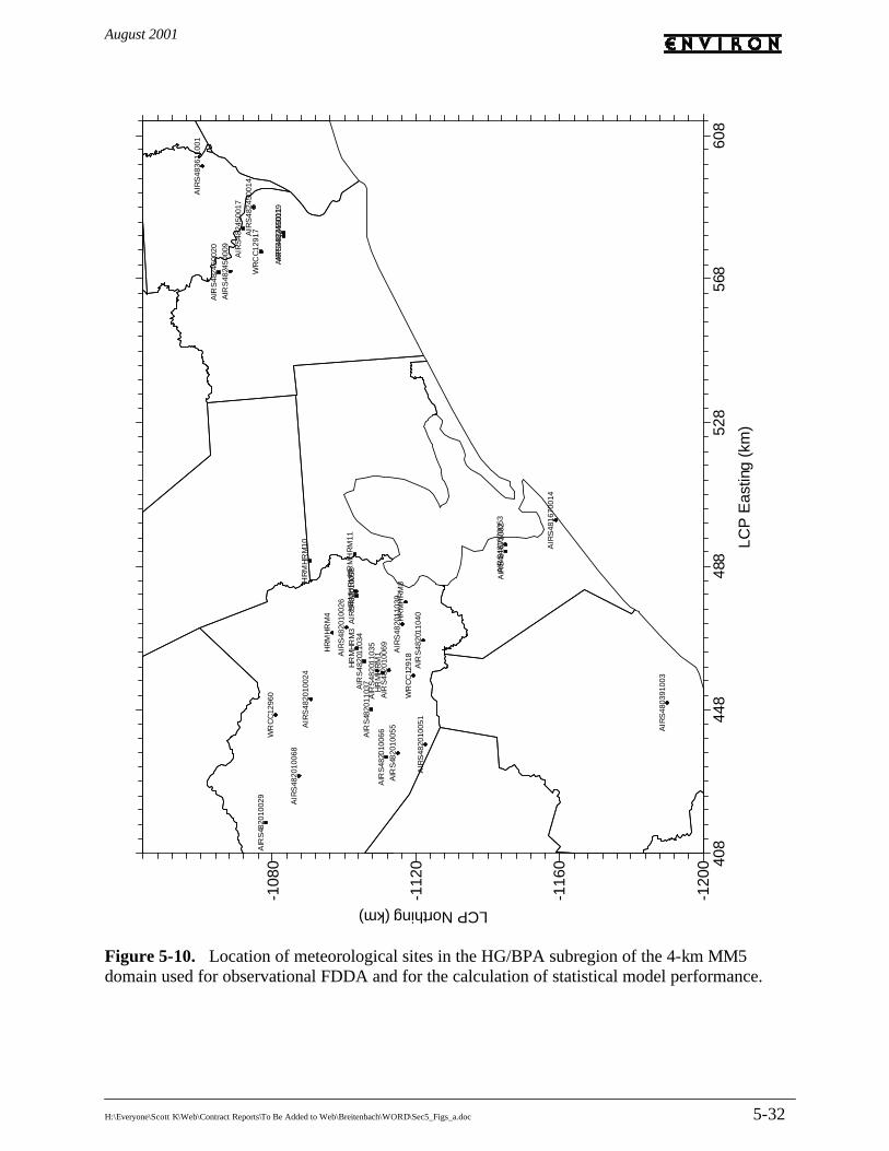
August 2001


Figure 5-10. Location of meteorological sites in the HG/BPA subregion of the 4-km MM5 domain used for observational FDDA and for the calculation of statistical model performance.

AIR

S48

0391

003

AIR

S48

1670

014

AIR

S48

1670

053

AIR

S48

1671

002

AIR

S48

2010

024

AIR

S48

2010

026

AIR

S48

2010

029

AIR

S48

2010

051

AIR

S48

2010

055

AIR

S48

2010

058

AIR

S48

2010

066

AIR

S48

2010

068

AIR

S48

2010

069

AIR

S48

2011

034

AIR

S48

2011

035

AIR

S48

2011

037

AIR

S48

2011

039

AIR

S48

2011

040

AIR

S48

2450

009

AIR

S48

2450

011

AIR

S48

2450

014

AIR

S48

2450

017

AIR

S48

2450

019

AIR

S48

2450

020

AIR

S48

3611

001

HR

MH

RM

1

HR

MH

RM

10

HR

MH

RM

11H

RM

HR

M3

HR

MH

RM

4

HR

MH

RM

7

HR

MH

RM

8

WR

CC

1291

7

WR

CC

1291

8

WR

CC

1296

0

408

448

488

528

568

608

LCP

Eas

ting

(km

)

-120

0

-116

0

-112

0

-108

0

LCP Northing (km)

August 2001


Figure 5-11. Location of meteorological sites over the 4-km DFW MM5 domain used for observational FDDA and for the calculation of statistical model performance.

AIRS480850005

AIRS481130057

AIRS481130069

AIRS481130075

AIRS481130087

AIRS481131006

AIRS481210034

AIRS481210054

AIRS481390015

AIRS481390016

AIRS484390057

AIRS484391002

AIRS484392003

RAOB72249WRCC13911

WRCC13960

WRCC13961

WRCC3927

168 208 248 288 328 368

LCP Easting (km)

-876

-836

-796

-756

-716

-676

LCP

Nor

thin

g (k

m)

August 2001

H:\Everyone\Scott K\Web\Contract Reports\To Be Added to Web\Breitenbach\WORD\Sec5_Figs_b.doc 5-34

Figure 5-12a. Hourly region-average observed and predicted (Run 1) surface-layer winds and performance statistics in the 12-km MM5 domain over the August 1999 modeling episode. RMSE is shown for total, systematic (RMSES) and unsystematic (RMSEU) components.


0123456

8/13 8/14 8/15 8/16 8/17 8/18 8/19 8/20 8/21 8/22

m/s

ObsWndSpd PrdWndSpd

Bias Windspeed

-3-2-1012

8/13 8/14 8/15 8/16 8/17 8/18 8/19 8/20 8/21 8/22

m/s

BiasWndSpd

RMSE Windspeed

00.5

11.5

22.5

3

8/13 8/14 8/15 8/16 8/17 8/18 8/19 8/20 8/21 8/22

m/s


IOA Windspeed

00.20.40.60.8

1

8/13 8/14 8/15 8/16 8/17 8/18 8/19 8/20 8/21 8/22

IOAWndSpd


060

120180240300360

8/13 8/14 8/15 8/16 8/17 8/18 8/19 8/20 8/21 8/22

de

g

ObsWndDir PrdWndDir

Bias Wind Direction

-90-60-30

0306090

8/13 8/14 8/15 8/16 8/17 8/18 8/19 8/20 8/21 8/22

de

g

BiasWndDir

August 2001


Figure 5-12b. Hourly region-average observed and predicted (Run 1) surface-layer temperature and performance statistics in the 12-km MM5 domain over the August 1999 modeling episode. RMSE is shown for total, systematic (RMSES) and unsystematic (RMSEU) components.


285

290

295

300

305

310

315

8/13 8/14 8/15 8/16 8/17 8/18 8/19 8/20 8/21 8/22

K

ObsTemp PrdTemp

Bias Temperature

-4

-3

-2

-1

0

1

2

3

4

8/13 8/14 8/15 8/16 8/17 8/18 8/19 8/20 8/21 8/22

K

BiasTemp

RMSE Temperature

00.5

11.5

22.5

33.5

44.5

5

8/13 8/14 8/15 8/16 8/17 8/18 8/19 8/20 8/21 8/22

K


IOA Temperature

00.10.20.30.40.50.60.70.80.9

1

8/13 8/14 8/15 8/16 8/17 8/18 8/19 8/20 8/21 8/22

IOATemp

August 2001


Figure 5-12c. Hourly region-average observed and predicted (Run 1) surface-layer humidity and performance statistics in the 12-km MM5 domain over the August 1999 modeling episode. RMSE is shown for total, systematic (RMSES) and unsystematic (RMSEU) components.


0

5

10

15

20

25

8/13 8/14 8/15 8/16 8/17 8/18 8/19 8/20 8/21 8/22

g/k

g

ObsHum PrdHum

Bias Humidity

-1

-0.5

0

0.5

1

1.5

2

2.5

3

8/13 8/14 8/15 8/16 8/17 8/18 8/19 8/20 8/21 8/22

g/k

g

BiasHum

RMSE Humidity

00.5

11.5

22.5

33.5

44.5

5

8/13 8/14 8/15 8/16 8/17 8/18 8/19 8/20 8/21 8/22

g/k

g


IOA Humidity

00.10.20.30.40.50.60.70.80.9

1

8/13 8/14 8/15 8/16 8/17 8/18 8/19 8/20 8/21 8/22

IOAHum

August 2001


Figure 5-13a. Daily region-average observed and predicted (Run 1) surface-layer winds and performance statistics in the 12-km MM5 domain over the August 1999 modeling episode. RMSE is shown for total, systematic and unsystematic components.


0

1

2

3

4

8/13 8/14 8/15 8/16 8/17 8/18 8/19 8/20 8/21 8/22

m/s

Wind Spd Mean OBS Wind Spd Mean PRD


-0.5

0

0.5

1

1.5

2

8/13 8/14 8/15 8/16 8/17 8/18 8/19 8/20 8/21 8/22

m/s


RMSE Windspeed

0

0.5

1

1.5

2

2.5

8/13 8/14 8/15 8/16 8/17 8/18 8/19 8/20 8/21 8/22

m/s


IOA Windspeed

0

0.2

0.4

0.6

0.8

1

8/13 8/14 8/15 8/16 8/17 8/18 8/19 8/20 8/21 8/22

Wind Spd IOA


0

60

120

180

240

300

360

8/13 8/14 8/15 8/16 8/17 8/18 8/19 8/20 8/21 8/22

de

g


Bias/Gross Error Wind Direction

-90

-60

-30

0

30

60

90

8/13 8/14 8/15 8/16 8/17 8/18 8/19 8/20 8/21 8/22

de

g


August 2001


Figure 5-13b. Daily region-average observed and predicted (Run 1) surface-layer temperature and performance statistics in the 12-km MM5 domain over the August 1999 modeling episode. RMSE is shown for total, systematic and unsystematic components.


300.5

301

301.5

302

302.5

303

303.5

304

304.5

8/13 8/14 8/15 8/16 8/17 8/18 8/19 8/20 8/21 8/22

K



-1

-0.5

0

0.5

1

1.5

2

2.5

8/13 8/14 8/15 8/16 8/17 8/18 8/19 8/20 8/21 8/22

K


RMSE Temperature

0

0.5

1

1.5

2

2.5

3

8/13 8/14 8/15 8/16 8/17 8/18 8/19 8/20 8/21 8/22

K


IOA Temperature

0

0.1

0.2

0.3

0.4

0.5

0.6

0.7

0.8

0.9

1

8/13 8/14 8/15 8/16 8/17 8/18 8/19 8/20 8/21 8/22

Temprtr IOA

August 2001


Figure 5-13c. Daily region-average observed and predicted (Run 1) surface-layer humidity and performance statistics in the 12-km MM5 domain over the August 1999 modeling episode. RMSE is shown for total, systematic and unsystema tic components.


0

2

4

6

8

10

12

14

16

18

20

8/13 8/14 8/15 8/16 8/17 8/18 8/19 8/20 8/21 8/22

g/k

g



0

0.5

1

1.5

2

2.5

3

3.5

8/13 8/14 8/15 8/16 8/17 8/18 8/19 8/20 8/21 8/22

g/k

g


RMSE Humidity

0

0.5

1

1.5

2

2.5

3

3.5

4

8/13 8/14 8/15 8/16 8/17 8/18 8/19 8/20 8/21 8/22

g/k

g


IOA Humidity

0

0.1

0.2

0.3

0.4

0.5

0.6

0.7

0.8

0.9

1

8/13 8/14 8/15 8/16 8/17 8/18 8/19 8/20 8/21 8/22

Humdity IOA

August 2001


Figure 5-14a. Comparison of Run 1 and Run 2 daily region-average performance statistics for winds in the 12-km MM5 domain over the August 1999 modeling episode.

Bias Wind Speed

-0.6

-0.4

-0.2

0

0.2

0.4

0.6

0.8

8/13 8/14 8/15 8/16 8/17 8/18 8/19 8/20 8/21 8/22

m/s

ETCOG 12-km Run 1 ETCOG 12-km Run 2

Gross Error Wind Speed

1.2

1.3

1.4

1.5

1.6

1.7

8/13 8/14 8/15 8/16 8/17 8/18 8/19 8/20 8/21 8/22

m/s


Total RMSE Wind Speed

0

0.5

1

1.5

2

2.5

8/13 8/14 8/15 8/16 8/17 8/18 8/19 8/20 8/21 8/22

m/s


IOA Speed

0

0.2

0.4

0.6

0.8

1

8/13 8/14 8/15 8/16 8/17 8/18 8/19 8/20 8/21 8/22


Bias Wind Direction

-20

-15

-10

-5

0

5

10

15

8/13 8/14 8/15 8/16 8/17 8/18 8/19 8/20 8/21 8/22

de

g


Gross Error Wind Direction

0

10

20

30

40

50

60

70

8/13 8/14 8/15 8/16 8/17 8/18 8/19 8/20 8/21 8/22

de

g


August 2001


Figure 5-14b. Comparison of Run 1 and Run 2 daily region-average performance statistics for temperature in the 12-km MM5 domain over the August 1999 modeling episode.

Bias Temperature

-0.6

-0.4

-0.2

0

0.2

0.4

0.6

0.8

8/13 8/14 8/15 8/16 8/17 8/18 8/19 8/20 8/21 8/22

K


Gross Error Temperature

0

0.5

1

1.5

2

2.5

8/13 8/14 8/15 8/16 8/17 8/18 8/19 8/20 8/21 8/22

K


Total RMSE Temperature

0

0.5

1

1.5

2

2.5

3

8/13 8/14 8/15 8/16 8/17 8/18 8/19 8/20 8/21 8/22

K


IOA Temperature

0

0.1

0.2

0.3

0.4

0.5

0.6

0.7

0.8

0.9

1

8/13 8/14 8/15 8/16 8/17 8/18 8/19 8/20 8/21 8/22


August 2001


Figure 5-14c. Comparison of Run 1 and Run 2 daily region-average performance statistics for humidity in the 12-km MM5 domain over the August 1999 modeling episode.

Bias Humidity

0

0.2

0.4

0.6

0.8

1

1.2

1.4

1.6

1.8

2

8/13 8/14 8/15 8/16 8/17 8/18 8/19 8/20 8/21 8/22

g/k

g


Gross Error Humidity

0

0.5

1

1.5

2

2.5

3

3.5

8/13 8/14 8/15 8/16 8/17 8/18 8/19 8/20 8/21 8/22

g/k

g


Total RMSE Humidity

0

0.5

1

1.5

2

2.5

3

3.5

4

8/13 8/14 8/15 8/16 8/17 8/18 8/19 8/20 8/21 8/22

g/k

g


IOA Humidity

0

0.1

0.2

0.3

0.4

0.5

0.6

0.7

0.8

0.9

1

8/13 8/14 8/15 8/16 8/17 8/18 8/19 8/20 8/21 8/22


August 2001


Figure 5-15a. Hourly region-average observed and predicted (Run 1) surface-layer winds and performance statistics in the 4-km DFW MM5 domain over the August 1999 modeling episode. RMSE is shown for total, systematic (RMSES) and unsystematic (RMSEU) components.


0

2

4

6

8

8/13 8/14 8/15 8/16 8/17 8/18 8/19 8/20 8/21 8/22

m/s

ObsWndSpd PrdWndSpd

Bias Windspeed

-4

-2

0

2

4

8/13 8/14 8/15 8/16 8/17 8/18 8/19 8/20 8/21 8/22

m/s

BiasWndSpd

RMSE Windspeed

012345

8/13 8/14 8/15 8/16 8/17 8/18 8/19 8/20 8/21 8/22

m/s


IOA Windspeed

00.20.40.60.8

1

8/13 8/14 8/15 8/16 8/17 8/18 8/19 8/20 8/21 8/22

IOAWndSpd


060

120180240300360

8/13 8/14 8/15 8/16 8/17 8/18 8/19 8/20 8/21 8/22

de

g

ObsWndDir PrdWndDir

Bias Wind Direction

-90-60-30

0306090

8/13 8/14 8/15 8/16 8/17 8/18 8/19 8/20 8/21 8/22

de

g

BiasWndDir

August 2001


Figure 5-15b. Hourly region-average observed and predicted (Run 1) surface-layer temperature and performance statistics in the 4-km DFW MM5 domain over the August 1999 modeling episode. RMSE is shown for total, systematic (RMSES) and unsystematic (RMSEU) components.


285

290

295

300

305

310

315

8/13 8/14 8/15 8/16 8/17 8/18 8/19 8/20 8/21 8/22

K

ObsTemp PrdTemp

Bias Temperature

-4

-3-2

-10

12

34

5

8/13 8/14 8/15 8/16 8/17 8/18 8/19 8/20 8/21 8/22

K

BiasTemp

RMSE Temperature

00.5

11.5

22.5

33.5

44.5

8/13 8/14 8/15 8/16 8/17 8/18 8/19 8/20 8/21 8/22

K


IOA Temperature

00.10.20.30.40.50.60.70.80.9

1

8/13 8/14 8/15 8/16 8/17 8/18 8/19 8/20 8/21 8/22

IOATemp

August 2001


Figure 5-15c. Hourly region-average observed and predicted (Run 1) surface-layer humidity and performance statistics in the 4-km DFW MM5 domain over the August 1999 modeling episode. RMSE is shown for total, systematic (RMSES) and unsystematic (RMSEU) components.


0

5

10

15

20

25

8/13 8/14 8/15 8/16 8/17 8/18 8/19 8/20 8/21 8/22

g/k

g

ObsHum PrdHum

Bias Humidity

-8

-6

-4

-2

0

2

4

6

8

8/13 8/14 8/15 8/16 8/17 8/18 8/19 8/20 8/21 8/22

g/k

g

BiasHum

RMSE Humidity

0

1

2

3

4

5

6

7

8/13 8/14 8/15 8/16 8/17 8/18 8/19 8/20 8/21 8/22

g/k

g


IOA Humidity

00.10.20.30.40.50.60.70.80.9

1

8/13 8/14 8/15 8/16 8/17 8/18 8/19 8/20 8/21 8/22

IOAHum

August 2001


Figure 5-16a. Daily region-average observed and predicted (Run 1) surface-layer winds and performance statistics in the 4-km DFW MM5 domain over the August 1999 modeling episode. RMSE is shown for total, systematic and unsystematic components.


0

1

2

3

4

5

8/13 8/14 8/15 8/16 8/17 8/18 8/19 8/20 8/21 8/22

m/s



-1-0.5

00.5

11.5

22.5

8/13 8/14 8/15 8/16 8/17 8/18 8/19 8/20 8/21 8/22

m/s


RMSE Windspeed

0

0.5

1

1.5

2

2.5

8/13 8/14 8/15 8/16 8/17 8/18 8/19 8/20 8/21 8/22

m/s


IOA Windspeed

0

0.2

0.4

0.6

0.8

1

8/13 8/14 8/15 8/16 8/17 8/18 8/19 8/20 8/21 8/22

Wind Spd IOA


0

60

120

180

240

300

360

8/13 8/14 8/15 8/16 8/17 8/18 8/19 8/20 8/21 8/22

de

g



-90

-60

-30

0

30

60

90

8/13 8/14 8/15 8/16 8/17 8/18 8/19 8/20 8/21 8/22

de

g


August 2001


Figure 5-16b. Daily region-average observed and predicted (Run 1) surface-layer temperature and performance statistics in the 4-km DFW MM5 domain over the August 1999 modeling episode. RMSE is shown for total, systematic and unsystematic components.


299

300

301

302

303

304

305

306

307

8/13 8/14 8/15 8/16 8/17 8/18 8/19 8/20 8/21 8/22

K



-2.5

-2

-1.5

-1

-0.5

0

0.5

1

1.5

2

2.5

8/13 8/14 8/15 8/16 8/17 8/18 8/19 8/20 8/21 8/22

K


RMSE Temperature

0

0.5

1

1.5

2

2.5

3

8/13 8/14 8/15 8/16 8/17 8/18 8/19 8/20 8/21 8/22

K


IOA Temperature

0

0.1

0.2

0.3

0.4

0.5

0.6

0.7

0.8

0.9

1

8/13 8/14 8/15 8/16 8/17 8/18 8/19 8/20 8/21 8/22

Temprtr IOA

August 2001


Figure 5-16c. Daily region-average observed and predicted (Run 1) surface-layer humidity and performance statistics in the 4-km DFW MM5 domain over the August 1999 modeling episode. RMSE is shown for total, systematic and unsystematic components.


0

2

4

6

8

10

12

14

16

18

20

8/13 8/14 8/15 8/16 8/17 8/18 8/19 8/20 8/21 8/22

g/k

g



-2

-1

0

1

2

3

4

5

8/13 8/14 8/15 8/16 8/17 8/18 8/19 8/20 8/21 8/22

g/k

g


RMSE Humidity

0

1

2

3

4

5

6

8/13 8/14 8/15 8/16 8/17 8/18 8/19 8/20 8/21 8/22

g/k

g


IOA Humidity

0

0.1

0.2

0.3

0.4

0.5

0.6

0.7

0.8

0.9

1

8/13 8/14 8/15 8/16 8/17 8/18 8/19 8/20 8/21 8/22

Humdity IOA

August 2001


Figure 5-17. Comparison of Run 1 and Run 2 daily region-average performance statistics for winds in the 4-km DFW MM5 domain over the August 1999 modeling episode.

Bias Wind Speed

-1.5

-1

-0.5

0

0.5

1

1.5

8/13 8/14 8/15 8/16 8/17 8/18 8/19 8/20 8/21 8/22

m/s

DFW 04-km Run 1 DFW 04-km Run 2


0

0.5

1

1.5

2

8/13 8/14 8/15 8/16 8/17 8/18 8/19 8/20 8/21 8/22

m/s



0

0.5

1

1.5

2

2.5

8/13 8/14 8/15 8/16 8/17 8/18 8/19 8/20 8/21 8/22

m/s


IOA Speed

0

0.2

0.4

0.6

0.8

1

8/13 8/14 8/15 8/16 8/17 8/18 8/19 8/20 8/21 8/22


Bias Wind Direction

-20

-10

0

10

20

30

8/13 8/14 8/15 8/16 8/17 8/18 8/19 8/20 8/21 8/22

de

g



0

20

40

60

80

100

8/13 8/14 8/15 8/16 8/17 8/18 8/19 8/20 8/21 8/22

de

g


August 2001


Figure 5-18a. Hourly region-average observed and predicted (Run 1) surface-layer winds and performance statistics in the 12-km MM5 domain over the September 1999 modeling episode. RMSE is shown for total, systematic (RMSES) and unsystematic (RMSEU) components.


012345

9/13 9/14 9/15 9/16 9/17 9/18 9/19 9/20

m/s

ObsWndSpd PrdWndSpd

Bias Windspeed

-3-2-10123

9/13 9/14 9/15 9/16 9/17 9/18 9/19 9/20

m/s

BiasWndSpd

RMSE Windspeed

00.5

11.5

22.5

3

9/13 9/14 9/15 9/16 9/17 9/18 9/19 9/20

m/s


IOA Windspeed

00.20.40.60.8

1

9/13 9/14 9/15 9/16 9/17 9/18 9/19 9/20

IOAWndSpd


060

120180240300360

9/13 9/14 9/15 9/16 9/17 9/18 9/19 9/20

de

g

ObsWndDir PrdWndDir

Bias Wind Direction

-90-60-30

0306090

9/13 9/14 9/15 9/16 9/17 9/18 9/19 9/20

de

g

BiasWndDir

August 2001


Figure 5-18b. Hourly region-average observed and predicted (Run 1) surface-layer temperature and performance statistics in the 12-km MM5 domain over the September 1999 modeling episode. RMSE is shown for total, systematic (RMSES) and unsystematic (RMSEU) components.


280

285

290

295

300

305

310

9/13 9/14 9/15 9/16 9/17 9/18 9/19 9/20

K

ObsTemp PrdTemp

Bias Temperature

-4

-3

-2

-1

0

1

2

3

9/13 9/14 9/15 9/16 9/17 9/18 9/19 9/20

K

BiasTemp

RMSE Temperature

0

0.5

1

1.5

2

2.5

3

3.5

9/13 9/14 9/15 9/16 9/17 9/18 9/19 9/20

K


IOA Temperature

00.10.20.30.40.50.60.70.80.9

1

9/13 9/14 9/15 9/16 9/17 9/18 9/19 9/20

IOATemp

August 2001


Figure 5-18c. Hourly region-average observed and predicted (Run 1) surface-layer humidity and performance statistics in the 12-km MM5 domain over the September 1999 modeling episode. RMSE is shown for total, systematic (RMSES) and unsystematic (RMSEU) components.


0

246

810

1214

1618

9/13 9/14 9/15 9/16 9/17 9/18 9/19 9/20

g/k

g

ObsHum PrdHum

Bias Humidity

-1

-0.5

0

0.5

1

1.5

2

9/13 9/14 9/15 9/16 9/17 9/18 9/19 9/20

g/k

g

BiasHum

RMSE Humidity

0

0.5

1

1.5

2

2.5

3

9/13 9/14 9/15 9/16 9/17 9/18 9/19 9/20

g/k

g


IOA Humidity

00.10.20.30.40.50.60.70.80.9

1

9/13 9/14 9/15 9/16 9/17 9/18 9/19 9/20

IOAHum

August 2001


Figure 5-19a. Daily region-average observed and predicted (Run 1) surface-layer winds and performance statistics in the 12-km MM5 domain over the September 1999 modeling episode. RMSE is shown for total, systematic and unsystematic components.


0

1

2

3

4

9/13 9/14 9/15 9/16 9/17 9/18 9/19 9/20

m/s



-1

-0.5

0

0.5

1

1.5

2

9/13 9/14 9/15 9/16 9/17 9/18 9/19 9/20

m/s


RMSE Windspeed

0

0.5

1

1.5

2

2.5

9/13 9/14 9/15 9/16 9/17 9/18 9/19 9/20

m/s


IOA Windspeed

0

0.2

0.4

0.6

0.8

1

9/13 9/14 9/15 9/16 9/17 9/18 9/19 9/20

Wind Spd IOA


0

60

120

180

240

300

360

9/13 9/14 9/15 9/16 9/17 9/18 9/19 9/20

de

g



-90

-60

-30

0

30

60

90

9/13 9/14 9/15 9/16 9/17 9/18 9/19 9/20

de

g


August 2001


Figure 5-19b. Daily region-average observed and predicted (Run 1) surface-layer temperature and performance statistics in the 12-km MM5 domain over the September 1999 modeling episode. RMSE is shown for total, systematic and unsystematic components.


294.5

295

295.5

296

296.5

297

297.5

298

298.5

299

299.5

300

9/13 9/14 9/15 9/16 9/17 9/18 9/19 9/20

K



-2

-1.5

-1

-0.5

0

0.5

1

1.5

2

2.5

9/13 9/14 9/15 9/16 9/17 9/18 9/19 9/20

K


RMSE Temperature

0

0.5

1

1.5

2

2.5

3

9/13 9/14 9/15 9/16 9/17 9/18 9/19 9/20

K


IOA Temperature

0

0.1

0.2

0.3

0.4

0.5

0.6

0.7

0.8

0.9

1

9/13 9/14 9/15 9/16 9/17 9/18 9/19 9/20

Temprtr IOA

August 2001


Figure 5-19c. Daily region-average observed and predicted (Run 1) surface-layer humidity and performance statistics in the 12-km MM5 domain over the September 1999 modeling episode. RMSE is shown for total, systematic and unsystematic components.


0

2

4

6

8

10

12

14

16

9/13 9/14 9/15 9/16 9/17 9/18 9/19 9/20

g/k

g



-0.5

0

0.5

1

1.5

2

9/13 9/14 9/15 9/16 9/17 9/18 9/19 9/20

g/k

g


RMSE Humidity

0

0.5

1

1.5

2

2.5

9/13 9/14 9/15 9/16 9/17 9/18 9/19 9/20

g/k

g


IOA Humidity

0

0.1

0.2

0.3

0.4

0.5

0.6

0.7

0.8

0.9

1

9/13 9/14 9/15 9/16 9/17 9/18 9/19 9/20

Humdity IOA

August 2001


Figure 5-20. Comparison of Run 1 and Run 2 daily region-average performance statistics for winds in the 12-km MM5 domain over the September 1999 modeling episode.

Bias Wind Speed

-1

-0.5

0

0.5

1

1.5

9/13 9/14 9/15 9/16 9/17 9/18 9/19 9/20

m/s

TXNNA 12-km Run 1 TXNNA 12-km Run 2


1.3

1.4

1.5

1.6

1.7

1.8

9/13 9/14 9/15 9/16 9/17 9/18 9/19 9/20

m/s



1.6

1.7

1.8

1.9

2

2.1

2.2

9/13 9/14 9/15 9/16 9/17 9/18 9/19 9/20

m/s


IOA Speed

0

0.2

0.4

0.6

0.8

1

9/13 9/14 9/15 9/16 9/17 9/18 9/19 9/20


Bias Wind Direction

-15

-10

-5

0

5

10

15

20

9/13 9/14 9/15 9/16 9/17 9/18 9/19 9/20

de

g



0

10

20

30

40

50

60

70

9/13 9/14 9/15 9/16 9/17 9/18 9/19 9/20

de

g


August 2001


Figure 5-21a. Hourly region-average observed and predicted (Run 1) surface-layer winds and performance statistics in the HG/BPA subregion of the 4-km MM5 domain over the September 1999 modeling episode. RMSE is shown for total, systematic (RMSES) and unsystematic (RMSEU) components.


0123456

9/13 9/14 9/15 9/16 9/17 9/18 9/19 9/20

m/s

ObsWndSpd PrdWndSpd

Bias Windspeed

-3-2-10123

9/13 9/14 9/15 9/16 9/17 9/18 9/19 9/20

m/s

BiasWndSpd

RMSE Windspeed

00.5

11.5

22.5

3

9/13 9/14 9/15 9/16 9/17 9/18 9/19 9/20

m/s


IOA Windspeed

00.20.40.60.8

1

9/13 9/14 9/15 9/16 9/17 9/18 9/19 9/20

IOAWndSpd


060

120180240300360

9/13 9/14 9/15 9/16 9/17 9/18 9/19 9/20

de

g

ObsWndDir PrdWndDir

Bias Wind Direction

-90-60-30

0306090

9/13 9/14 9/15 9/16 9/17 9/18 9/19 9/20

de

g

BiasWndDir

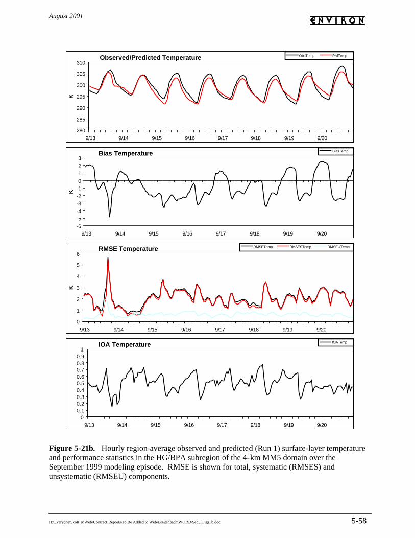
August 2001


Figure 5-21b. Hourly region-average observed and predicted (Run 1) surface-layer temperature and performance statistics in the HG/BPA subregion of the 4-km MM5 domain over the September 1999 modeling episode. RMSE is shown for total, systematic (RMSES) and unsystematic (RMSEU) components.


280

285

290

295

300

305

310

9/13 9/14 9/15 9/16 9/17 9/18 9/19 9/20

K

ObsTemp PrdTemp

Bias Temperature

-6

-5-4

-3-2

-10

12

3

9/13 9/14 9/15 9/16 9/17 9/18 9/19 9/20

K

BiasTemp

RMSE Temperature

0

1

2

3

4

5

6

9/13 9/14 9/15 9/16 9/17 9/18 9/19 9/20

K


IOA Temperature

00.10.20.30.40.50.60.70.80.9

1

9/13 9/14 9/15 9/16 9/17 9/18 9/19 9/20

IOATemp

August 2001


Figure 5-22a. Daily region-average observed and predicted (Run 1) surface-layer winds and performance statistics in the HG/BPA subregion of the 4-km MM5 domain over the September 1999 modeling episode. RMSE is shown for total, systematic and unsystematic components.


0

1

2

3

4

5

9/13 9/14 9/15 9/16 9/17 9/18 9/19 9/20

m/s



0

0.5

1

1.5

2

9/13 9/14 9/15 9/16 9/17 9/18 9/19 9/20

m/s


RMSE Windspeed

0

0.5

1

1.5

2

2.5

9/13 9/14 9/15 9/16 9/17 9/18 9/19 9/20

m/s


IOA Windspeed

0

0.2

0.4

0.6

0.8

1

9/13 9/14 9/15 9/16 9/17 9/18 9/19 9/20

Wind Spd IOA


0

60

120

180

240

300

360

9/13 9/14 9/15 9/16 9/17 9/18 9/19 9/20

de

g



-90

-60

-30

0

30

60

90

9/13 9/14 9/15 9/16 9/17 9/18 9/19 9/20

de

g


August 2001


Figure 5-22b. Daily region-average observed and predicted (Run 1) surface-layer temperature and performance statistics in the HG/BPA subregion of the 4-km MM5 domain over the September 1999 modeling episode. RMSE is shown for total, systematic and unsystematic components.


295

296

297

298

299

300

301

302

9/13 9/14 9/15 9/16 9/17 9/18 9/19 9/20

K



-3

-2

-1

0

1

2

3

9/13 9/14 9/15 9/16 9/17 9/18 9/19 9/20

K


RMSE Temperature

0

0.5

1

1.5

2

2.5

3

9/13 9/14 9/15 9/16 9/17 9/18 9/19 9/20

K


IOA Temperature

0

0.1

0.2

0.3

0.4

0.5

0.6

0.7

0.8

0.9

1

9/13 9/14 9/15 9/16 9/17 9/18 9/19 9/20

Temprtr IOA

August 2001


Figure 5-23a. Comparison of Run 1 and Run 2 daily region-average performance statistics for winds in the HG/BPA subregion of the 4-km MM5 domain over the September 1999 modeling episode.

Bias Wind Speed

-0.5

0

0.5

1

1.5

2

9/13 9/14 9/15 9/16 9/17 9/18 9/19 9/20

m/s

HGBPA Run 1 HGBPA Run 2


0

0.5

1

1.5

2

9/13 9/14 9/15 9/16 9/17 9/18 9/19 9/20

m/s



0

0.5

1

1.5

2

2.5

9/13 9/14 9/15 9/16 9/17 9/18 9/19 9/20

m/s


IOA Speed

0

0.2

0.4

0.6

0.8

1

9/13 9/14 9/15 9/16 9/17 9/18 9/19 9/20


Bias Wind Direction

-20

-10

0

10

20

30

40

50

9/13 9/14 9/15 9/16 9/17 9/18 9/19 9/20

de

g



0

20

40

60

80

9/13 9/14 9/15 9/16 9/17 9/18 9/19 9/20

de

g


August 2001


Figure 5-23b. Comparison of Run 1 and Run 2 daily region-average performance statistics for temperature in the HG/BPA subregion of the 4-km MM5 domain over the September 1999 modeling episode.

Bias Temperature

-2.5

-2

-1.5

-1

-0.5

0

0.5

9/13 9/14 9/15 9/16 9/17 9/18 9/19 9/20

K



0

0.5

1

1.5

2

2.5

3

9/13 9/14 9/15 9/16 9/17 9/18 9/19 9/20

K



0

0.5

1

1.5

2

2.5

3

9/13 9/14 9/15 9/16 9/17 9/18 9/19 9/20

K


IOA Temperature

0

0.1

0.2

0.3

0.4

0.5

0.6

0.7

0.8

0.9

1

9/13 9/14 9/15 9/16 9/17 9/18 9/19 9/20


August 2001


6. SENSITIVITY MODELING Results from the Base Case simulations described in the previous section illustrated two basic MM5 performance issues in both DFW and HG/BPA episodes/domains: (1) the damping of the diurnal temperature wave, and (2) excessive wind speeds at night. A simple thought experiment can link these two problems together along with a lesser third issue, namely the over prediction of humidity in the boundary layer. The thought is this: the damped diurnal temperature wave could be related to excessive surface moisture content, which would serve to increase the thermal inertia of the soil (thereby lowering maximum temperatures and raising minimum temperatures). High soil moisture would also lead to a large surface moisture flux to the atmosphere, resulting in over predictions in boundary layer humidity. This in turn would lead to an insulating effect during the night, where the higher humidity increases the infrared feedback to the surface, further diminishing the cooling rate. The higher nocturnal temperatures would not allow the surface to sufficiently decouple from layers aloft, which could allow winds to more readily mix toward the ground (leading to over predictions in speed during the night). Since these processes are so closely linked, this argument also works in reverse, resulting in a “chicken-egg” paradox. However, there is no clearly obvious mechanism to explain why low-level nocturnal wind speeds are accelerated as they are in these simulations. The MM5 has exhibited this characteristic in many other applications that ENVIRON and others have undertaken the past few years, as mentioned in Section 5. Two additional sensitivity simulations were designed: Run 3) An additional data assimilation run, similar to Base Case Run 2, except that the

observational nudging coefficients were increased to 1×10-3 s-1 on both 12- and 4-km grids (an increase by a factor of 2.5 over the Run 2 nudging strengths). The test will indicate the extent to which the erroneously high nocturnal surface winds and low daytime winds can be artificially controlled via nudging to actual data, and how that influences temperature performance (especially at night). The reader should understand that, if successful, this run merely represents a “patch” for a potentially serious deficiency in MM5, and that the underlying cause for poor wind performance is not rectified;

Run 4) Similar to Run 3, except that the soil moisture and thermal inertia were reduced over

all land cover types (except water and wetlands, details are given below). This test will indicate the sensitivity of MM5 to the choice of important soil parameters in controlling surface temperature, near-surface nocturnal stability, and boundary layer humidity.

Results described below primarily focus on the simulations on the 4-km grids. RUN 3: STRONGER NUDGING COEFFICIENTS August 1999 Episode Figure 6-1 presents the hourly domain-averaged time series for winds, temperature, and humidity in the DFW 4-km grid. Inspection of the wind speed time series (Figure 6-1a) does not indicate

August 2001


any significant performance improvements with the introduction of stronger nudging coefficients. Compared to Run 2 (see Figure 5-15) the same under predictions of daytime speed occurs, most likely a result of the weaker pressure gradient developed in this area by MM5 than observed. Some marginal improvements in wind direction are apparent, except on August 17. There is no evidence of any change in diurnal temperature performance, and only slight changes in humidity (Figure 6-1 b and c). Figure 6-2 presents the daily performance statistics for the DFW grid. These results are shown along with Run 1 and 2 for reference. While the daily bias in wind speed indicates some marginal improvement in Run 3, the gross error, total RMSE, and IOA show a definite improvement with the introduction of stronger nudging (Figure 6-2a). Results for directional bias are mixed, but tend toward a slight improvement as well. Relatively dramatic improvements are seen for directional gross error with all days brought to within 45 degrees. Very small and mixed results are seen for daily temperature and humidity statistics (Figure 6-2 b and c). Similar hourly and daily results were seen on the 12-km grid (not shown) for this episode. Overall, the effect of stronger observational nudging coefficients for winds result in lower speed and direction errors. However, the impact of a 2.5-fold increase in the nudging strength was surprisingly minimal for wind speed. A comparison of the daily statistics shown in Figure 6-2 for Run 3 with the proposed benchmarks established in Section 4 is shown in the tabulation below. Those measures that exceed the benchmarks are shown in red. Values with asterisks denote degradation in performance relative to Run 2. Parameter Benchmark Run 3 Range Run 3 Episode-Mean Wind Speed RMSE 2.0 1.1 1.9 1.5 Wind Speed Bias --- -0.9 0.7 -0.2 Wind Speed IOA 0.6 0.28 0.73 0.48 Wind Direction Gross Error 20 14 48 30 Wind Direction Bias --- *-20 21 3 Temperature Bias ±0.5 -2.0 0.9* -0.9 Temperature Gross Error 2.0 1.4 2.1 1.7 Temperature IOA 0.7 *0.86 0.95 0.92 Humidity Bias ±1.0 -0.7 3.8 0.9 Humidity Gross Error 2.0 1.3 4.3 2.0 Humidity IOA 0.7 *0.34 0.81* 0.53 Very little change is seen in the overall statistics for winds, certainly not enough to move all wind statistics into the benchmark ranges. Some slight but insignificant degradation in temperature bias, temperature IOA, and humidity IOA are noted. September 1999 Episode Figure 6-3 shows the hourly domain-average statistics for wind and temperature in the HG/BPA sub-domain, and humidity in the entire 4-km domain (recall that insufficient humidity measurements are available in the HG/BPA domain). Comparing the wind performa nce to Run 2 (Figure 5-21), it is clear that improvements occur for both speed and direction over the modeling episode. The amplitude of over and under predictions is reduced, as indicated by a smaller range in bias. A slight improvement in wind direction is most notable late in the period. However, heavier wind data nudging is not dramatically improving the performance issues

August 2001


identified in Section 5. Again, only very small changes are evident in the temperature and humidity figures. Daily statistical results are shown in Figure 6-4. At the daily scale, the improvements to wind speed in the HG/BPA area are clear, with definite improvements in bias, gross error, total RMSE, and IOA (although bias shows larger negative values on September 19 and 20). Gross error approaches an episode-mean of 1 m/s. Wind direction similarly shows good improvement for bias and gross error, especially on the last two days of the episode. Gross error is brought to within 45 degrees over the entire episode. Interestingly, there are small improvements in daily temperature bias over the entire episode, but mixed results for the absolute error metrics. The likely cause of this is that lower mean wind speed arising from the stronger nudging is decreasing the turbulent sensible heat flux away from the surface, thereby slightly increasing the temperatures overall and reducing the negative bias. While differences in the humidity metrics arise over the entire 4-km grid when winds are more strongly nudged, they are a mixture of improvements and degradations. A comparison of the daily statistics shown in Figure 6-4 for Run 3 with the proposed benchmarks established in Section 4 is shown in the tabulation below. Those measures that exceed the benchmarks are shown in red. Values with asterisks denote degradation in performance relative to Run 2. Parameter Benchmark Run 3 Range Run 3 Episode-Mean Wind Speed RMSE 2.0 1.3 1.7 1.5 Wind Speed Bias --- *-0.3 1.3 0.5 Wind Speed IOA 0.6 0.35 0.66 0.49 Wind Direction Gross Error 20 14 46 31 Wind Direction Bias --- -10 18 -2 Temperature Bias ±0.5 -2.1 0.1 -0.6 Temperature Gross Error 2.0 1.0 2.2 1.8 Temperature IOA 0.7 0.88 0.96 0.92* Humidity Bias ±1.0 *-0.7 1.0 0.3 Humidity Gross Error 2.0 1.0 1.9* 1.6 Humidity IOA 0.7 *0.49 0.88 0.69 RUN 4: ALTERED SOIL PARAMETERS Discussions were held with Dr. Nelson Seaman at Pennsylvania State University (personal communication), co-author of MM5, regarding the temperature problems seen in results to this point in the study. Dr. Seaman suggested that the default soil moisture levels assigned to each landuse type might be too high for these episodes, and that it could be reduced by as much as 50% based on cases he has run. The soil moisture is one of several parameters that define the conditions of the soil as a function of landuse, and it has been seen that MM5 simulations are rather sensitive to this particular parameter. The default moisture is set for seasonal mean values, and therefore are probably unrepresentative of the drier conditions that set up during prolonged warm periods associated with poor ozone air quality in Texas. Recall that in the basic setup of MM5 for these applications, the single-slab Blackadar “force-restore” soil model was selected. This model is not interactive with precipitation and so does not

August 2001


account for the “history” of the soil conditions over an episode. A multi-layer model is also available, but it too does not have an interactive capability for moisture, and our past experience indicates that it does not necessarily lead to improved temperature performance over the single-slab model. The new multi-level land soil model (LSM) that is now available with MM5, and other versions to be added soon, do contain multiple layers and the ability to specify actual soil types (clay, sand, loam, etc.); they can be initialized for deep soil temperature and moisture from the large-scale analyses like EDAS and GDAS/Reanalysis datasets, and they are fully interactive with simulated precipitation. However, added complexity does not necessarily always lead to improved model performance, as accurate simulation of precipitation patterns, timing and intensity are even more crucial for a successful run. Furthermore, the need to specify initial conditions for several more important fields from coarse-resolution analyses adds another dimension of potential error. Nevertheless, we suggest that future applications of MM5 for these periods consider testing the impact of the multi-layer soil models. Based upon Dr. Seaman’s suggestion, we investigated the level of drought conditions existing in the south-central U.S. during August and September 1999. A particularly useful internet web site was found that is maintained by the National Drought Mitigation Center at the University of Nebraska (http://enso.unl.edu/ndmc/watch/spi99map.htm). The site presents maps of the Standardized Precipitation Index (SPI) analyzed for the various climate divisions defined by the National Climatic Data Center. This index provides a semi-quantitative description of the relative amount of precipitation each climate division has received over time periods ranging from one month to a full year. Examples for August and September 1999 are shown in Figures 6-5 and 6-6, respectively. Both 1-month and 3-month SPI maps are provided. Evaluation of these maps indicates that August 1999 was particularly dry throughout the south and midwest U.S. from a climatological perspective. Since the 3-month SPI ending in August is close to normal in the south-central U.S., it would appear that June and July received average or just above average precipitation. The single month of September does not appear as dry as August over the southern U.S., but south-central Texas is drier than usual. Note that the 3-month SPI ending in September is particularly dry due to the influence of August. These maps support the idea that the seasonal average soil moisture defined in MM5 should be reduced by some extent. Unfortunately, no information was found from which a quantitative reduction factor could be directly applied. Table 6-1 shows the default MM5 soil moisture content as a function of the 24-category USGS landuse types utilized in this study. In an initial trial application in which only the 2-way nested 108/36/12-km domains were run, these moisture values were cut in half (except for water and wetlands) to gauge the response of the model in both episodes. Results from this test (not shown) clearly showed over predictions in daily temperature and under predictions in boundary layer humidity. The diurnal temperature wave was simply shifted upwards by about 5 K (i.e., there was no expansion of the amplitude of the temperature wave), and the under predictions in humidity about equaled the over predictions in MM5 runs up to this point. Therefore, a new tact was defined for Run 4. First, the soil moisture content was reduced by only 25% (see Table 6-1). Second, to address the need to amplify the diurnal temperature wave rather than simply shifting it higher, the soil thermal inertia was arbitrarily reduced as well (Table 6-1). These modifications were added to the setup for Run 3 (stronger wind observation nudging). Table 6-1. MM5 default and altered soil parameters in the USGS 24-category dataset. Landuse types in bold were not modified.

MM5 Default Modified Run 4

August 2001


Landuse Type

Moisture Availability

(%)

Thermal Inertia (cal cm-2 K-1 s-1/2)

Moisture Availability

(%)

Thermal Inertia (cal cm-2 K-1 s-1/2)

Urban 10 0.03 7 0.02 Dryland Crop, Pasture 30 0.04 23 0.03 Irrigated Crop, Pasture 50 0.04 40 0.03 Mixed Dry/Irrigated Crop, Pasture 25 0.04 20 0.03 Crop/Grassland Mosaic 25 0.04 18 0.03 Crop/Woodland Mosaic 35 0.04 25 0.03 Grassland 15 0.03 11 0.02 Shrubland 10 0.03 7 0.02 Mixed Shrub/Grassland 15 0.03 11 0.02 Savanna 15 0.03 11 0.02 Decidous Broadleaf 30 0.04 23 0.03 Decidous Needle 30 0.04 23 0.03 Evergreen Broadleaf 50 0.05 37 0.04 Evergreen Needle 30 0.04 23 0.03 Mixed Forest 30 0.04 23 0.03 Water Body 100 0.06 100 0.06 Herbaceous Wetland 60 0.06 60 0.06 Wooden Tundra 35 0.05 35 0.05 Bare/Sparse Vegetation 2 0.02 1 0.01 Herbaceous Tundra 50 0.05 37 0.04 Wooden Tundra 50 0.05 37 0.04 Mixed Tundra 50 0.05 37 0.04 Bare Ground Tundra 2 0.02 1 0.01 Snow/Ice 95 0.05 95 0.05

August 1999 Episode Figure 6-7 presents the Run 4 hourly domain-averaged time series for winds, temperature, and humidity in the DFW 4-km grid. Comparison of the wind speed trends to those of Run 3 (Figure 6-1) does not reveal any significant impacts, but hourly directional error is improved noticeably. The hourly temperature results are plotted with the Run 3 results overlaid for more direct comparison. Daily peak temperatures are better replicated in Run 4 (except on the first day), and the overall impact appears to be a better simulation during daylight hours. Minimum temperatures in Run 4 remain very close to Run 3, which for the DFW area were not as high as for other areas/periods. A particularly warm night is simulated on August 19-20, and the reasons for this are not obvious. The modifications made to soil parameters appear to be quite reasonable given these results. The hourly humidity in Run 4 is generally lower than in Run 3, but the model does not exhibit any improved skill in replicating the intra-daily variations, especially toward the end of the episode (see for example, the IOA). The lower humidity appears to have led to an improved hourly bias trace. Daily statistical results in the DFW grid are shown in Figure 6-8. Again, little impact is seen for wind speed, although bias and error are somewhat improved toward the end of the episode. The wind direction bias shows mixed results in Run 4 relative to Runs 2 and 3, but the gross error is further reduced during the days with the poorest performance, and all daily error is within 40 degrees. As expected, the most dramatic improvements are seen for temperature, where on most days the under prediction bias is improved to about –0.5 K. On days in which temperature was performing well (August 19 and 20), the modifications to soil parameters has led to over predictions of 1 to 1.5 K (mainly due to the high nocturnal temperatures on these days). Gross error is reduced to about 1 K on most days, and the total RMSE is reduced to about 1.5 K. As a

August 2001


result, IOA is increase to well over 0.9 on many days of the episode. The overall impact on humidity includes some dramatic improvements in bias and error on the worst performing days, and only marginal improvements in IOA. A comparison of the daily statistics shown in Figure 6-8 for Run 4 with the proposed benchmarks established in Section 4 is shown in the tabulation below. Those measures that exceed the benchmarks are shown in red. Values with asterisks denote degradation in performance relative to Run 3. Parameter Benchmark Run 4 Range Run 4 Episode-Mean Wind Speed RMSE 2.0 *1.3 1.9 1.5 Wind Speed Bias --- -0.7 0.7 -0.2 Wind Speed IOA 0.6 0.34 0.73 0.49 Wind Direction Gross Error 20 *15 42 29 Wind Direction Bias --- -15 22* 6* Temperature Bias ±0.5 -1.0 1.9* -0.1 Temperature Gross Error 2.0 1.0 2.3* 1.4 Temperature IOA 0.7 0.86 0.97 0.94 Humidity Bias ±1.0 *-2.1 2.3 0.1 Humidity Gross Error 2.0 1.1 3.0 1.9 Humidity IOA 0.7 0.38 0.75* 0.55 For this episode, it would appear that the reduction in soil moisture, and possibly an adjustment to the thermal inertia, is warranted. Overall temperature and humidity bias and error are improved, even though their respective episodic ranges are increased slightly. September 1999 Episode Figure 6-9 shows the hourly domain-average statistics for wind and temperature in the HG/BPA sub-domain, and humidity in the entire 4-km south-central Texas domain. As was the case for DFW, the soil modifications made in Run 4 do not appear to have any significant impact on wind speed or direction. This is particularly surprising since it was expected that warming of the coastal regions would induce a more definite sea breeze circulation, and so more changes would be seen in directional performance for HG/BPA than for DFW. The impact to hourly temperatures are similar to the DFW results, in that most of the temperature improvements are seen during the daytime hours and little impact is seen on the early morning minimum temperatures. The bias is reduced substantially from Run 3 during daytime hours. For humidity on the entire 4-km grid, Run 4 results in a downward shift of the hourly time series by about 1 g/kg, but it is not clear that bias and error are improved any, and like DFW, there is no increase in the hour-to-hour skill in replicated intra-diurnal humidity patterns. Figure 6-10 presents the daily statistics for winds and temperature in the HG/BPA sub-domain and for humidity in the entire 4-km grid. While not obvious in the hourly results, the daily statistics show a definite improvement in wind speed bias and error over the previous MM5 runs. The results for wind direction bias and error are also generally better, especially on the last few days of the episode. So the larger expected impacts on HG/BPA winds compared to DFW are apparent, and are made more clear in the daily results. Like the DFW results, the improvements to daily temperature bias are dramatic, and only the last two days show increased bias because of rather good performance in the previous runs. Gross error and RMSE are improved by a quarter

August 2001


to half a degree, and IOA is increased to 0.95 on most days. The impacts on humidity bias are mixed, leading to some relatively large negative values on some days that were performing well in the previous runs. Overall error and RMSE are improved on most days by a few tenths of a g/kg. The humidity IOA is improved on all but the first two (spinup) days of the episode. A comparison of the daily statistics shown in Figure 6-10 for Run 4 with the proposed benchmarks established in Section 4 is shown in the tabulation below. Those measures that exceed the benchmarks are shown in red. Values with asterisks denote degradation in performance relative to Run 3. Parameter Benchmark Run 4 Range Run 4 Episode-Mean Wind Speed RMSE 2.0 1.2 1.6 1.4 Wind Speed Bias --- -0.3 1.2 0.3 Wind Speed IOA 0.6 0.41 0.69 0.51 Wind Direction Gross Error 20 14 42 27 Wind Direction Bias --- -8 11 -2 Temperature Bias ±0.5 -1.7 0.5* -0.3 Temperature Gross Error 2.0 *1.1 1.8 1.5 Temperature IOA 0.7 0.89 0.96 0.94 Humidity Bias ±1.0 *-1.4 0.7 -0.3 Humidity Gross Error 2.0 *1.3 1.9 1.5 Humidity IOA 0.7 0.55 0.86* 0.74 Considering the results of Run 4 for this episode in the HG/BPA area, it appears that a surface modification is warranted. However, the benefits to humidity are not as clear as they are for DFW and this is probably related to the coastal environment. Recall from Figures 6-5 and 6-6 that Texas was not as severely dry in September as in August. Therefore, it is also possible that a reduction in surface moisture by 25% is too large for September. The change to thermal inertia, in combination with the reduced soil moisture, appears adequate for improving the temperature performance. IMPACTS ON RESOLVED FLOW FIELDS The successive MM5 applications from Run 1 through Run 4 have incrementally improved the performance in winds in both DFW and HG/BPA. Recall that Run 2 added observational nudging toward hourly wind measurements in the 12- and 4-km grid, while Run 3 increased the nudging strength by a factor of 2.5. Finally, the modifications to soil parameters made in Run 4 had little impact on winds in DFW, but a larger impact on winds in HG/BPA. Conceptually, the improved and warmer land-surface temperatures in the HG/BPA area induced a stronger on-shore sea breeze component, which resulted in better agreement with the wind measurements. To illustrate the successive evolution of wind patterns along the Gulf coast in the 4-km south-central Texas grid, Figures 6-11 through 6-13 display the surface wind fields at 1800 CST on September 19 for Runs 1, 3, and 4. The entire set of plots are provided in a separate database. Note that at this particular time, MM5 Run 1 has produced a thin zone of on-shore flow along the Gulf coast and around the various bays (Figure 6-11). With the introduction of rather strong observational nudging in Run 3 (Figure 6-12), some evidence of a wider zone of onshore flow appears, especially in the Houston area where a large number of monitoring sites exist. Note that wind speeds remain light, but that the largest impact is on wind direction. In the final plot

August 2001


(Figure 6-13), a much wider sea breeze zone is apparent along the entire Gulf Coast, expanding both offshore and onshore. Again, wind speeds are not significantly affected, but the winds are rotated toward on-shore directions over a broader area. It would appear from these results, and from the statistical evaluation described above, that the successive modifications to the MM5 configuration in these runs are credible and warranted as they result in consistently improved results. We note, however, that additional improvements in the predicted wind fields are needed to bring the wind performance closer to the proposed benchmarks (i.e., to performance levels that have been achieved in other modeling applications as reported by Tesche et al., 2001b). This will be crucial to minimize the transport error that might occur in air quality models.

August 2001

tnrcc-loe\order11-mm5eval\Task4\Sec6_figs.doc 6-9



0

2

4

6

8

8/13 8/14 8/15 8/16 8/17 8/18 8/19 8/20 8/21 8/22

m/s

ObsWndSpd PrdWndSpd

Bias Windspeed

-4

-2

0

2

4

8/13 8/14 8/15 8/16 8/17 8/18 8/19 8/20 8/21 8/22

m/s

BiasWndSpd

RMSE Windspeed

0

1

2

3

4

8/13 8/14 8/15 8/16 8/17 8/18 8/19 8/20 8/21 8/22

m/s


IOA Windspeed

00.20.40.60.8

1

8/13 8/14 8/15 8/16 8/17 8/18 8/19 8/20 8/21 8/22

IOAWndSpd


060

120180240300360

8/13 8/14 8/15 8/16 8/17 8/18 8/19 8/20 8/21 8/22

de

g

ObsWndDir PrdWndDir

Bias Wind Direction

-90-60-30

0306090

8/13 8/14 8/15 8/16 8/17 8/18 8/19 8/20 8/21 8/22

de

g

BiasWndDir

August 2001


Figure 6-1b. Hourly region-average observed and predicted (Run 3) surface-layer temperature and performance statistics in the 4-km DFW MM5 domain over the August 1999 modeling episode. RMSE is shown for total, systematic (RMSES) and unsystematic (RMSEU) components.


285

290

295

300

305

310

315

8/13 8/14 8/15 8/16 8/17 8/18 8/19 8/20 8/21 8/22

K

ObsTemp PrdTemp

Bias Temperature

-4-3

-2-1

01

23

45

8/13 8/14 8/15 8/16 8/17 8/18 8/19 8/20 8/21 8/22

K

BiasTemp

RMSE Temperature

00.5

11.5

22.5

33.5

44.5

5

8/13 8/14 8/15 8/16 8/17 8/18 8/19 8/20 8/21 8/22

K


IOA Temperature

00.10.20.30.40.50.60.70.80.9

1

8/13 8/14 8/15 8/16 8/17 8/18 8/19 8/20 8/21 8/22

IOATemp

August 2001


Figure 6-1c. Hourly region-average observed and predicted (Run 3) surface-layer humidity and performance statistics in the 4-km DFW MM5 domain over the August 1999 modeling episode. RMSE is shown for total, systematic (RMSES) and unsystematic (RMSEU) components.


0

5

10

15

20

25

8/13 8/14 8/15 8/16 8/17 8/18 8/19 8/20 8/21 8/22

g/k

g

ObsHum PrdHum

Bias Humidity

-8

-6

-4

-2

0

2

4

6

8

8/13 8/14 8/15 8/16 8/17 8/18 8/19 8/20 8/21 8/22

g/k

g

BiasHum

RMSE Humidity

0

1

2

3

4

5

6

7

8/13 8/14 8/15 8/16 8/17 8/18 8/19 8/20 8/21 8/22

g/k

g


IOA Humidity

00.10.20.30.40.50.60.70.80.9

1

8/13 8/14 8/15 8/16 8/17 8/18 8/19 8/20 8/21 8/22

IOAHum

August 2001


Figure 6-2a. Comparison of Run 1, 2, and 3 daily region-average performance statistics for winds in the 4-km DFW MM5 domain over the August 1999 modeling episode.

Bias Wind Speed

-1.5

-1

-0.5

0

0.5

1

1.5

8/13 8/14 8/15 8/16 8/17 8/18 8/19 8/20 8/21 8/22

m/s

DFW 04-km Run 1 DFW 04-km Run 2 DFW 04-km Run 3


0

0.5

1

1.5

2

8/13 8/14 8/15 8/16 8/17 8/18 8/19 8/20 8/21 8/22

m/s



0

0.5

1

1.5

2

2.5

8/13 8/14 8/15 8/16 8/17 8/18 8/19 8/20 8/21 8/22

m/s


IOA Speed

0

0.2

0.4

0.6

0.8

1

8/13 8/14 8/15 8/16 8/17 8/18 8/19 8/20 8/21 8/22


Bias Wind Direction

-30

-20

-10

0

10

20

30

8/13 8/14 8/15 8/16 8/17 8/18 8/19 8/20 8/21 8/22

de

g



0

20

40

60

80

100

8/13 8/14 8/15 8/16 8/17 8/18 8/19 8/20 8/21 8/22

de

g


August 2001


Figure 6-2b. Comparison of Run 1, 2, and 3 daily region-average performance statistics for temperature in the 4-km DFW MM5 domain over the August 1999 modeling episode.

Bias Temperature

-2.5

-2

-1.5

-1

-0.5

0

0.5

1

1.5

8/13 8/14 8/15 8/16 8/17 8/18 8/19 8/20 8/21 8/22

K



0

0.5

1

1.5

2

2.5

8/13 8/14 8/15 8/16 8/17 8/18 8/19 8/20 8/21 8/22

K



0

0.5

1

1.5

2

2.5

3

8/13 8/14 8/15 8/16 8/17 8/18 8/19 8/20 8/21 8/22

K


IOA Temperature

0

0.1

0.2

0.3

0.4

0.5

0.6

0.7

0.8

0.9

1

8/13 8/14 8/15 8/16 8/17 8/18 8/19 8/20 8/21 8/22


August 2001


Figure 6-2c. Comparison of Run 1, 2, and 3 daily region-average performance statistics for humidity in the 4-km DFW MM5 domain over the August 1999 modeling episode.

Bias Humidity

-2

-1

0

1

2

3

4

5

8/13 8/14 8/15 8/16 8/17 8/18 8/19 8/20 8/21 8/22

g/k

g



0

0.5

1

1.5

2

2.5

3

3.5

4

4.5

5

8/13 8/14 8/15 8/16 8/17 8/18 8/19 8/20 8/21 8/22

g/k

g


Total RMSE Humidity

0

1

2

3

4

5

6

8/13 8/14 8/15 8/16 8/17 8/18 8/19 8/20 8/21 8/22

g/k

g


IOA Humidity

0

0.1

0.2

0.3

0.4

0.5

0.6

0.7

0.8

0.9

1

8/13 8/14 8/15 8/16 8/17 8/18 8/19 8/20 8/21 8/22


August 2001


Figure 6-3a. Hourly region-average observed and predicted (Run 3) surface-layer winds and performance statistics in the 4-km HG/BPA sub-domain over the September 1999 modeling episode. RMSE is shown for total, systematic (RMSES) and unsystematic (RMSEU) components.


0123456

9/13 9/14 9/15 9/16 9/17 9/18 9/19 9/20

m/s

ObsWndSpd PrdWndSpd

Bias Windspeed

-3-2-10123

9/13 9/14 9/15 9/16 9/17 9/18 9/19 9/20

m/s

BiasWndSpd

RMSE Windspeed

0

1

2

3

4

9/13 9/14 9/15 9/16 9/17 9/18 9/19 9/20

m/s


IOA Windspeed

00.20.40.60.8

1

9/13 9/14 9/15 9/16 9/17 9/18 9/19 9/20

IOAWndSpd


060

120180240300360

9/13 9/14 9/15 9/16 9/17 9/18 9/19 9/20

de

g

ObsWndDir PrdWndDir

Bias Wind Direction

-90-60-30

0306090

9/13 9/14 9/15 9/16 9/17 9/18 9/19 9/20

de

g

BiasWndDir

August 2001


Figure 6-3b. Hourly region-average observed and predicted (Run 3) surface-layer temperature and performance statistics in the 4-km HG/BPA sub-domain over the September 1999 modeling episode. RMSE is shown for total, systematic (RMSES) and unsystematic (RMSEU) components.


280

285

290

295

300

305

310

9/13 9/14 9/15 9/16 9/17 9/18 9/19 9/20

K

ObsTemp PrdTemp

Bias Temperature

-4

-3

-2

-1

0

1

2

3

9/13 9/14 9/15 9/16 9/17 9/18 9/19 9/20

K

BiasTemp

RMSE Temperature

00.5

11.5

22.5

33.5

44.5

5

9/13 9/14 9/15 9/16 9/17 9/18 9/19 9/20

K


IOA Temperature

00.10.20.30.40.50.60.70.80.9

1

9/13 9/14 9/15 9/16 9/17 9/18 9/19 9/20

IOATemp

August 2001


Figure 6-3c. Hourly region-average observed and predicted (Run 3) surface-layer humidity and performance statistics in the 4-km MM5 domain over the September 1999 modeling episode. RMSE is shown for total, systematic (RMSES) and unsystematic (RMSEU) components.


02468

101214161820

9/13 9/14 9/15 9/16 9/17 9/18 9/19 9/20

g/k

g

ObsHum PrdHum

Bias Humidity

-2-1.5

-1-0.5

00.5

11.5

22.5

33.5

9/13 9/14 9/15 9/16 9/17 9/18 9/19 9/20

g/k

g

BiasHum

RMSE Humidity

0

0.5

1

1.5

2

2.5

3

3.5

9/13 9/14 9/15 9/16 9/17 9/18 9/19 9/20

g/k

g


IOA Humidity

00.10.20.30.40.50.60.70.80.9

1

9/13 9/14 9/15 9/16 9/17 9/18 9/19 9/20

IOAHum

August 2001


Figure 6-4a. Comparison of Run 1, 2, and 3 daily region-average performance statistics for winds in the 4-km HG/BPA sub-domain over the September 1999 modeling episode.

Bias Wind Speed

-0.5

0

0.5

1

1.5

2

9/13 9/14 9/15 9/16 9/17 9/18 9/19 9/20

m/s

HGBPA Run 1 HGBPA Run 2 HGBPA Run 3


0

0.5

1

1.5

2

9/13 9/14 9/15 9/16 9/17 9/18 9/19 9/20

m/s



0

0.5

1

1.5

2

2.5

9/13 9/14 9/15 9/16 9/17 9/18 9/19 9/20

m/s


IOA Speed

0

0.2

0.4

0.6

0.8

1

9/13 9/14 9/15 9/16 9/17 9/18 9/19 9/20


Bias Wind Direction

-20

-10

0

10

20

30

40

50

9/13 9/14 9/15 9/16 9/17 9/18 9/19 9/20

de

g



0

20

40

60

80

9/13 9/14 9/15 9/16 9/17 9/18 9/19 9/20

de

g


August 2001


Figure 6-4b. Comparison of Run 1, 2, and 3 daily region-average performance statistics for temperature in the 4-km HG/BPA sub-domain over the September 1999 modeling episode.

Bias Temperature

-2.5

-2

-1.5

-1

-0.5

0

0.5

9/13 9/14 9/15 9/16 9/17 9/18 9/19 9/20

KHGBPA Run 1 HGBPA Run 2 HGBPA Run 3


0

0.5

1

1.5

2

2.5

3

9/13 9/14 9/15 9/16 9/17 9/18 9/19 9/20

K



0

0.5

1

1.5

2

2.5

3

9/13 9/14 9/15 9/16 9/17 9/18 9/19 9/20

K


IOA Temperature

0

0.1

0.2

0.3

0.4

0.5

0.6

0.7

0.8

0.9

1

9/13 9/14 9/15 9/16 9/17 9/18 9/19 9/20


August 2001


Figure 6-4c. Comparison of Run 1, 2, and 3 daily region-average performance statistics for humidity in the 4-km MM5 domain over the September 1999 modeling episode.

Bias Humidity

-1

-0.5

0

0.5

1

1.5

9/13 9/14 9/15 9/16 9/17 9/18 9/19 9/20

g/k

g

TXNNA 4-km Run 1 TXNNA 4-km Run 2 TXNNA 4-km Run 3


0

0.5

1

1.5

2

2.5

9/13 9/14 9/15 9/16 9/17 9/18 9/19 9/20

g/k

g


Total RMSE Humidity

0

0.5

1

1.5

2

2.5

3

9/13 9/14 9/15 9/16 9/17 9/18 9/19 9/20

g/k

g


IOA Humidity

0

0.1

0.2

0.3

0.4

0.5

0.6

0.7

0.8

0.9

1

9/13 9/14 9/15 9/16 9/17 9/18 9/19 9/20


August 2001


Figure 6-5. 1- and 3-month Standardized Precipitation Index ending in August 1999, indicating levels of drought relative to climatological norms in each climate zone.

August 2001


Figure 6-6. 1- and 3-month Standardized Precipitation Index ending in September 1999, indicating levels of drought relative to climatological norms in each climate zone.

August 2001




0

2

4

6

8

8/13 8/14 8/15 8/16 8/17 8/18 8/19 8/20 8/21 8/22

m/s

ObsWndSpd PrdWndSpd

Bias Windspeed

-4

-2

0

2

4

8/13 8/14 8/15 8/16 8/17 8/18 8/19 8/20 8/21 8/22

m/s

BiasWndSpd

RMSE Windspeed

0

1

2

3

4

8/13 8/14 8/15 8/16 8/17 8/18 8/19 8/20 8/21 8/22

m/s


IOA Windspeed

00.20.40.60.8

1

8/13 8/14 8/15 8/16 8/17 8/18 8/19 8/20 8/21 8/22

IOAWndSpd


060

120180240300360

8/13 8/14 8/15 8/16 8/17 8/18 8/19 8/20 8/21 8/22

de

g

ObsWndDir PrdWndDir

Bias Wind Direction

-90-60-30

0306090

8/13 8/14 8/15 8/16 8/17 8/18 8/19 8/20 8/21 8/22

de

g

BiasWndDir

August 2001


Figure 6-7b. Hourly region-average observed and predicted (Run 4) surface-layer temperature and performance statistics in the 4-km DFW MM5 domain over the August 1999 modeling episode. RMSE is shown for total, systematic (RMSES) and unsystematic (RMSEU) components. Results for Run 3 are overlaid in blue.


285

290

295

300

305

310

315

8/13 8/14 8/15 8/16 8/17 8/18 8/19 8/20 8/21 8/22

KObsTemp PrdTemp Run 3

Bias Temperature

-5-4-3-2-1012345

8/13 8/14 8/15 8/16 8/17 8/18 8/19 8/20 8/21 8/22

K

BiasTemp Run 3

RMSE Temperature

00.5

11.5

22.5

33.5

44.5

5

8/13 8/14 8/15 8/16 8/17 8/18 8/19 8/20 8/21 8/22

K


IOA Temperature

00.10.20.30.40.50.60.70.80.9

1

8/13 8/14 8/15 8/16 8/17 8/18 8/19 8/20 8/21 8/22

IOATemp

August 2001


Figure 6-7c. Hourly region-average observed and predicted (Run 4) surface-layer humidity and performance statistics in the 4-km DFW MM5 domain over the August 1999 modeling episode. RMSE is shown for total, systematic (RMSES) and unsystematic (RMSEU) components. Results for Run 3 are overlaid in blue.


0

5

10

15

20

25

8/13 8/14 8/15 8/16 8/17 8/18 8/19 8/20 8/21 8/22

g/k

g

ObsHum PrdHum Run 3

Bias Humidity

-10-8

-6-4

-20

24

68

8/13 8/14 8/15 8/16 8/17 8/18 8/19 8/20 8/21 8/22

g/k

g

BiasHum Run 3

RMSE Humidity

0

12

34

56

78

9

8/13 8/14 8/15 8/16 8/17 8/18 8/19 8/20 8/21 8/22

g/k

g


IOA Humidity

00.10.20.30.40.50.60.70.80.9

1

8/13 8/14 8/15 8/16 8/17 8/18 8/19 8/20 8/21 8/22

IOAHum

August 2001


Figure 6-8a. Comparison of Run 2, 3, and 4 daily region-average performance statistics for winds in the 4-km DFW MM5 domain over the August 1999 modeling episode.

Bias Wind Speed

-1.5

-1

-0.5

0

0.5

1

8/13 8/14 8/15 8/16 8/17 8/18 8/19 8/20 8/21 8/22

m/s



0

0.5

1

1.5

2

8/13 8/14 8/15 8/16 8/17 8/18 8/19 8/20 8/21 8/22

m/s



0

0.5

1

1.5

2

2.5

8/13 8/14 8/15 8/16 8/17 8/18 8/19 8/20 8/21 8/22

m/s


IOA Speed

0

0.2

0.4

0.6

0.8

1

8/13 8/14 8/15 8/16 8/17 8/18 8/19 8/20 8/21 8/22


Bias Wind Direction

-30

-20

-10

0

10

20

30

8/13 8/14 8/15 8/16 8/17 8/18 8/19 8/20 8/21 8/22

de

g



0

20

40

60

80

8/13 8/14 8/15 8/16 8/17 8/18 8/19 8/20 8/21 8/22

de

g


August 2001


Figure 6-8b. Comparison of Run 2, 3, and 4 daily region-average performance statistics for temperature in the 4-km DFW MM5 domain over the August 1999 modeling episode.

Bias Temperature

-2.5

-2

-1.5

-1

-0.5

0

0.5

1

1.5

2

2.5

8/13 8/14 8/15 8/16 8/17 8/18 8/19 8/20 8/21 8/22

K



0

0.5

1

1.5

2

2.5

8/13 8/14 8/15 8/16 8/17 8/18 8/19 8/20 8/21 8/22

K



0

0.5

1

1.5

2

2.5

3

8/13 8/14 8/15 8/16 8/17 8/18 8/19 8/20 8/21 8/22

K


IOA Temperature

0

0.1

0.2

0.3

0.4

0.5

0.6

0.7

0.8

0.9

1

8/13 8/14 8/15 8/16 8/17 8/18 8/19 8/20 8/21 8/22


August 2001


Figure 6-8c. Comparison of Run 2, 3, and 4 daily region-average performance statistics for humidity in the 4-km DFW MM5 domain over the August 1999 modeling episode.

Bias Humidity

-3

-2

-1

0

1

2

3

4

5

8/13 8/14 8/15 8/16 8/17 8/18 8/19 8/20 8/21 8/22

g/k

g



0

0.5

1

1.5

2

2.5

3

3.5

4

4.5

5

8/13 8/14 8/15 8/16 8/17 8/18 8/19 8/20 8/21 8/22

g/k

g


Total RMSE Humidity

0

1

2

3

4

5

6

8/13 8/14 8/15 8/16 8/17 8/18 8/19 8/20 8/21 8/22

g/k

g


IOA Humidity

0

0.1

0.2

0.3

0.4

0.5

0.6

0.7

0.8

0.9

1

8/13 8/14 8/15 8/16 8/17 8/18 8/19 8/20 8/21 8/22


August 2001


Figure 6-9a. Hourly region-average observed and predicted (Run 4) surface-layer winds and performance statistics in the 4-km HG/BPA sub-domain over the September 1999 modeling episode. RMSE is shown for total, systematic (RMSES) and unsystematic (RMSEU) components. Results for Run 3 are overlaid in blue.


012345

9/13 9/14 9/15 9/16 9/17 9/18 9/19 9/20

m/s

ObsWndSpd PrdWndSpd Run 3

Bias Windspeed

-2-10123

9/13 9/14 9/15 9/16 9/17 9/18 9/19 9/20

m/s

BiasWndSpd Run 3

RMSE Windspeed

00.5

11.5

22.5

3

9/13 9/14 9/15 9/16 9/17 9/18 9/19 9/20

m/s


IOA Windspeed

00.20.40.60.8

1

9/13 9/14 9/15 9/16 9/17 9/18 9/19 9/20

IOAWndSpd


060

120180240300360

9/13 9/14 9/15 9/16 9/17 9/18 9/19 9/20

de

g

ObsWndDir PrdWndDir Run 3

Bias Wind Direction

-90-60-30

0306090

9/13 9/14 9/15 9/16 9/17 9/18 9/19 9/20

de

g

BiasWndDir Run 3

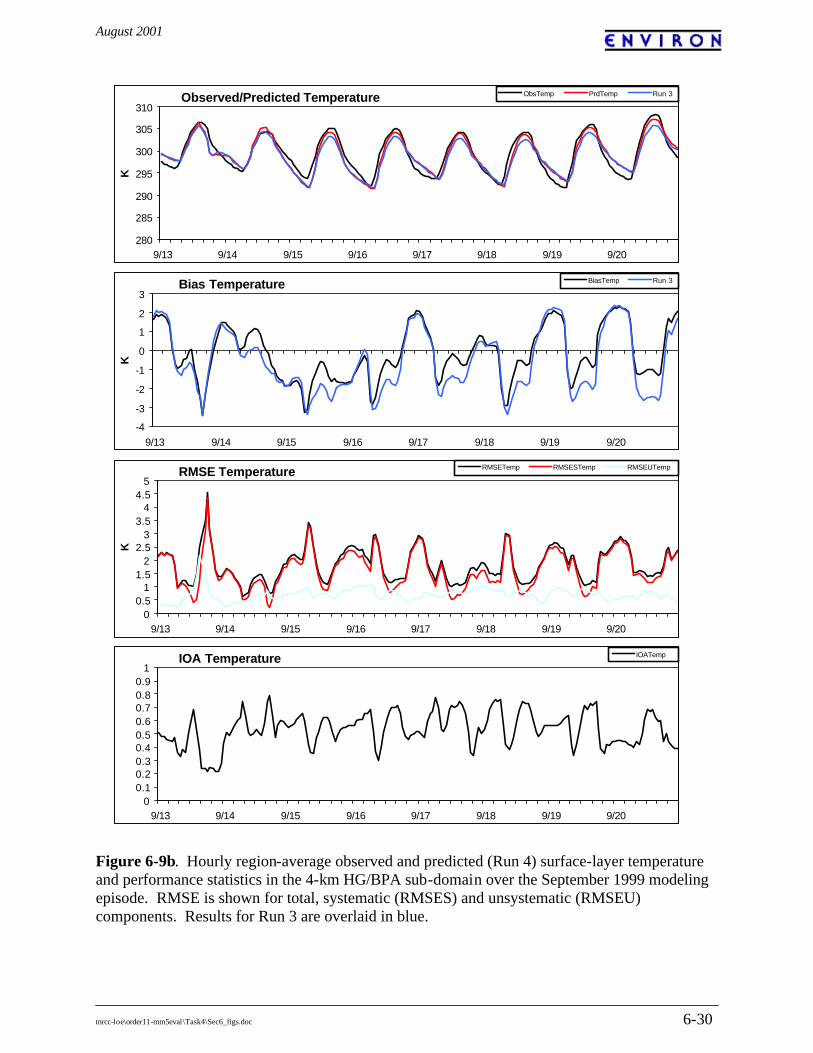
August 2001


Figure 6-9b. Hourly region-average observed and predicted (Run 4) surface-layer temperature and performance statistics in the 4-km HG/BPA sub-domain over the September 1999 modeling episode. RMSE is shown for total, systematic (RMSES) and unsystematic (RMSEU) components. Results for Run 3 are overlaid in blue.


280

285

290

295

300

305

310

9/13 9/14 9/15 9/16 9/17 9/18 9/19 9/20

K

ObsTemp PrdTemp Run 3

Bias Temperature

-4

-3

-2

-1

0

1

2

3

9/13 9/14 9/15 9/16 9/17 9/18 9/19 9/20

K

BiasTemp Run 3

RMSE Temperature

00.5

11.5

22.5

33.5

44.5

5

9/13 9/14 9/15 9/16 9/17 9/18 9/19 9/20

K


IOA Temperature

00.10.20.30.40.50.60.70.80.9

1

9/13 9/14 9/15 9/16 9/17 9/18 9/19 9/20

IOATemp

August 2001


Figure 6-9c. Hourly region-average observed and predicted (Run 4) surface-layer winds and performance statistics in the 4-km MM5 domain over the September 1999 modeling episode. RMSE is shown for total, systematic (RMSES) and unsystematic (RMSEU) components. Results for Run 3 are overlaid in blue.


02468

101214161820

9/13 9/14 9/15 9/16 9/17 9/18 9/19 9/20

g/k

g

ObsHum PrdHum Run 3

Bias Humidity

-3

-2

-1

0

1

2

3

4

9/13 9/14 9/15 9/16 9/17 9/18 9/19 9/20

g/k

g

BiasHum Run 3

RMSE Humidity

0

0.5

1

1.5

2

2.5

3

3.5

9/13 9/14 9/15 9/16 9/17 9/18 9/19 9/20

g/k

g


IOA Humidity

00.10.20.30.40.50.60.70.80.9

1

9/13 9/14 9/15 9/16 9/17 9/18 9/19 9/20

IOAHum

August 2001


Figure 6-10a. Comparison of Run 2, 3, and 4 daily region-average performance statistics for winds in the 4-km HG/BPA sub-domain over the September 1999 modeling episode.

Bias Wind Speed

-0.5

0

0.5

1

1.5

9/13 9/14 9/15 9/16 9/17 9/18 9/19 9/20

m/s



0

0.5

1

1.5

2

9/13 9/14 9/15 9/16 9/17 9/18 9/19 9/20

m/s



0

0.5

1

1.5

2

9/13 9/14 9/15 9/16 9/17 9/18 9/19 9/20

m/s


IOA Speed

0

0.2

0.4

0.6

0.8

1

9/13 9/14 9/15 9/16 9/17 9/18 9/19 9/20


Bias Wind Direction

-20

-10

0

10

20

30

9/13 9/14 9/15 9/16 9/17 9/18 9/19 9/20

de

g



0

10

20

30

40

50

60

9/13 9/14 9/15 9/16 9/17 9/18 9/19 9/20

de

g


August 2001


Figure 6-10b. Comparison of Run 2, 3, and 4 daily region-average performance statistics for temperature in the 4-km HG/BPA sub-domain over the September 1999 modeling episode.

Bias Temperature

-2.5

-2

-1.5

-1

-0.5

0

0.5

1

9/13 9/14 9/15 9/16 9/17 9/18 9/19 9/20

K



0

0.5

1

1.5

2

2.5

9/13 9/14 9/15 9/16 9/17 9/18 9/19 9/20

K



0

0.5

1

1.5

2

2.5

3

9/13 9/14 9/15 9/16 9/17 9/18 9/19 9/20

K


IOA Temperature

0

0.1

0.2

0.3

0.4

0.5

0.6

0.7

0.8

0.9

1

9/13 9/14 9/15 9/16 9/17 9/18 9/19 9/20


August 2001


Figure 6-10c. Comparison of Run 2, 3, and 4 daily region-average performance statistics for humidity in the 4-km MM5 domain over the September 1999 modeling episode.

Bias Humidity

-2

-1.5

-1

-0.5

0

0.5

1

1.5

9/13 9/14 9/15 9/16 9/17 9/18 9/19 9/20

g/k

g



0

0.2

0.4

0.6

0.8

1

1.2

1.4

1.6

1.8

2

9/13 9/14 9/15 9/16 9/17 9/18 9/19 9/20

g/k

g


Total RMSE Humidity

0

0.5

1

1.5

2

2.5

3

9/13 9/14 9/15 9/16 9/17 9/18 9/19 9/20

g/k

g


IOA Humidity

0

0.1

0.2

0.3

0.4

0.5

0.6

0.7

0.8

0.9

1

9/13 9/14 9/15 9/16 9/17 9/18 9/19 9/20


August 2001


Figure 6-11. Distribution of Run 1 surface-level winds in the south-central Texas 4-km MM5 domain on September 19, 1800 CST.

August 2001



August 2001


7. CONCLUSIONS The TRNCC has sponsored an MM5 modeling study that expands current modeling being performed for the Texas NNAs into the HG/BPA and DFW areas. The periods modeled include August 13-22, 1999 for the northern and eastern portion of Texas (i.e., East Texas and DFW), and September 13-20, 1999 for the south-central portion of Texas (i.e., Austin, San Antonio, Victoria, Corpus Christi, and HG/BPA). The quality of a meteorological simulation plays a crucial role in the accuracy of the air quality modeling results. Past applications of various meteorological modeling platforms have all indicated that certain areas of Texas, and certain episodes, are more difficult to replicate than others. In particular, the HG/BPA exercises in the past have demonstrated that the Galveston Bay Area is rather difficult to model, given complex interactions between sea, bay, and land breezes, and this has resulted in significant technical issues surrounding past photochemical modeling of that area. Past meteorological model evaluation procedures have been based upon rather subjective comparisons between observations and predicted fields of winds and temperatures. Thus, they have shed little light on the reasons for poor performance, and inter-comparisons with other modeling exercises have not benefited from a consistent evaluation methodology that compares results to established benchmarks for adequate performance. In order to systematically identify performance issues associated with difficult periods and/or areas to model, a quantitative objective assessment capability of MM5 performance needs to be developed, similar to the techniques employed for air quality modeling over the past ten years. The TNRCC identified two basic goals for the current study: 1) Exploiting the current meteorological modeling activities being performed for the NNAs,

expand the high-resolution 4-km modeling domains to include the HG/BPA and DFW areas and evaluate meteorological performance in those areas to assess the utility of future air quality modeling;

2) Establish performance evaluation procedures, statistics, and benchmarks for variables at the

surface and within the boundary layer, similar to performance goals set for photochemical modeling, so that the quality of these and future meteorological modeling applications can be evaluated and compared within a consistent and appropriate context.

The TNRCC intends to perform similar meteorological evaluations in all future photochemical modeling exercises, and to use the algorithms developed in this study in conjunction with sensitivity studies to optimize MM5 performance before relying on data nudging as a last resort. The development of statistical benchmarks should provide: (1) a way to gauge meteorological model performance relative to past exercises performed in the same areas of Texas and in other areas of the country; and (2) a means toward the long term goal of systematically improving meteorological modeling capabilities. The benchmarks should strike an adequate balance between the need to minimize allowable error, and the level to which MM5 (and other models such as RAMS) can be expected to perform. It is important to recognized that a given absolute wind error results in an increasing relative transport error in photochemical models as the model grid resolution increases. This is particularly important given the likely move toward ~1 km grid spacing to better resolve flow fields in the Houston area. It is entirely likely that striving for wind speed errors less than 1 m/s

August 2001


may well be beyond the state of the science of meteorological models at this time. However, if transport errors result in the displacement of pollutants by several grid squares, the regulatory modeling community needs to acknowledge the problem, and interpret photochemical model results while keeping the weaknesses of the meteorological models in mind. While it is well established that emission rate estimates are associated with an equal or greater level of error, there is as yet very little data to prove it one way or the other (i.e., errors can only be inferred from concentration data and questionable chemical responses in photochemical models). On the other hand, meteorological simulations can usually be evaluated against sufficient observational data to identify sources of input error. ESTABLISHMENT OF STATISTICAL BENCHMARKS In Section 4 we derived and proposed a set of preliminary performance “benchmarks” for typical meteorological model performance. These standards were based upon the evaluation of a variety of MM5 and RAMS applications in the last few years, as reported by Tesche et al. (2001b). The purpose of these benchmarks is not necessarily to give a passing or failing grade to any one particular meteorological model application, but rather to put its results into the proper context. For example, expectations for modeling of the Houston area might not be as high as a simpler domain such as DFW, for obvious reasons. The key to the benchmarks is to understand how poor or good the results are relative to the universe of other model applications run for Houston and other areas of the U.S. Certainly, an important criticism of the EPA guidance statistics for acceptable photochemical performance is that they are relied upon much too heavily to establish an acceptable (to the EPA) model simulation of a given area and episode. Often lost in the statistical evaluation is the need to critically evaluate all aspects of the model via diagnostic and process-oriented approaches. The same must stressed for the meteorological performance evaluation. In Section 4 it was noted that the appropriateness and adequacy of the proposed preliminary benchmarks would be carefully considered based upon the results of MM5 simulations performed and reported in this study. Based on these results, we have identified some necessary modifications. First and foremost, the proposed gross error in wind direction was based on an improper definition of this metric. The evaluation undertaken by Tesche et al. (2001b) actually reported the simple difference between domain- and episode-mean observed and predicted direction, which is a much more lenient approach (it usually leads to smaller “error”). In this study, we calculate an actual gross error statistic (the mean of hour-by-hour, site-by-site differences), which leads to much larger error values. Hence, the benchmark for this metric should be revised upward to reflect the different calculation methodology. Second, it is felt that a benchmark for bias should be added for wind speed and direction. Third, the proposed IOA benchmarks for humidity appear to be excessive, while the IOA for temperature appears to be too lenient. Unfortunately, the IOA for humidity and temperature were not reported by Tesche et al. (2001b), so we have based the revised values upon the results of the simulations reported here. Finally, a comment was received on the proposed benchmarks that requested the addition of gross error for wind speeds. However, since the more standard error measure for speed is RMSE, and values are usually quite similar to gross error, it was felt that having two absolute error statistics would be redundant.

August 2001


Based upon these considerations, the final proposed benchmarks are given below: Wind Speed RMSE: < 2 m/s Bias: < ±0.5 m/s (new) IOA: ≥ 0.6 Wind Direction Gross Error: < 30 deg (from 20) Bias: < ±10 deg (new) Temperature Gross Error: < 2 K Bias: < ±0.5 K IOA ≥ 0.8 (from 0.7) Humidity Gross Error: < 2 g/kg Bias: < ±1 g/kg IOA: ≥ 0.6 (from 0.7) Table 7-1 presents a recap of the episode-mean daily statistics determined for MM5 Runs 1 through 4 in the 4-km DFW grid over August 13-22, 1999. A similar summary is provided in Table 7-2 for the HG/BPA 4-km sub-domain over September 13-20, 1999 (the humidity statistics are calculated for the entire 4-km south-central Texas grid). Table 7-1. Episode-mean daily statistics from MM5 Runs 1 through 4 in the 4-km DFW grid over August 13-22, 1999. Red values denote statistics outside the final proposed benchmarks.

Benchmark Run 1 Run 2 Run 3 Run 4

Speed RMSE (m/s) 1.7 1.6 1.5 1.5 Speed Bias (m/s) -0.1 -0.2 -0.2 -0.2 Speed IOA 0.37 0.41 0.48 0.49 Direction Gross Error (deg) 43 36 30 29 Direction Bias (deg) 3 5 3 6 Temperature Gross Error (K) 1.8 1.7 1.7 1.4 Temperature Bias (K) -1.0 -0.9 -0.9 -0.1 Temperature IOA 0.92 0.92 0.92 0.94 Humidity Gross Error (g/kg) 2.0 2.0 2.0 1.9 Humidity Bias (g/kg) 0.9 0.9 0.9 0.1 Humidity IOA 0.53 0.53 0.53 0.55

August 2001


Table 7-1. Episode-mean daily statistics from MM5 Runs 1 through 4 in the 4-km HG/BPA sub-domain over August 13-22, 1999 (humidity from the entire 4-km south-central Texas grid). Red values denote statistics outside the proposed benchmarks. Benchmark Run 1 Run 2 Run 3 Run 4 Speed RMSE (m/s) 1.8 1.6 1.5 1.4 Speed Bias (m/s) 0.8 0.6 0.5 0.3 Speed IOA 0.39 0.44 0.49 0.51 Direction Gross Error (deg) 41 36 31 27 Direction Bias (deg) 1 -2 -2 -2 Temperature Gross Error (K) 1.8 1.8 1.8 1.5 Temperature Bias (K) -0.8 -0.7 -0.6 -0.3 Temperature IOA 0.93 0.93 0.92 0.94 Humidity Gross Error (g/kg) 1.7 1.6 1.6 1.5 Humidity Bias (g/kg) 0.4 0.4 0.3 -0.3 Humidity IOA 0.67 0.69 0.69 0.74

UTILITY OF MM5 SIMULATIONS FOR PHOTOCHEMICAL MODEL INPUT The MM5 applications run for this study show some promising results in replicating the large- and small-scale meteorology in the DFW and HG/BPA areas. Generally good performance is seen for wind direction, the placement of clouds and precipitation, and for temperature when appropriate modifications to soil parameters are made. Marginal performance is seen for humidity and the overall pressure pattern covering the south-central U.S. Some noted problems that remain throughout all runs include:

1) A consistent over prediction in wind speed at night (probably caused by an overly excited low level jet), and under predictions during the daytime (probably caused by the consistent over prediction of surface pressure over Texas), on all 4- and 12-km grids; and

2) A common over prediction tendency in early-morning temperatures, which is likely to

be related to a lack of near-surface nocturnal stabilization at night. There is a high probability that the nightly wind and temperature issues are interrelated. Although we have found no obvious clues as to which problem is the primary forcing, it would appear that some separate mechanism for exciting the nocturnal low-level jet phenomenon (which is common in this part of the country) is the cause for the high winds, and the resulting shear-induced mixing is maintaining the high early-morning temperatures. We have found that wind performance was only marginally improved when the nudging coefficients for the observational FDDA were increased by a rather large factor. However, significant improvements in temperature were found when soil moisture was adjusted to reflect the drier conditions of late summer 1999, and the thermal inertia parameter was reduced. Similar sensitivity could likely be seen if the multi-layer soil model, or the new LSM approach is used. Marginal improvements were seen in surface humidity with these changes, as were additional slight improvements to surface wind performance. At the very least, the change in soil moisture appears warranted for these applications. Given the remaining problems identified for wind speed, we cannot yet advocate the use of these

August 2001


MM5 results for SIP-quality photochemical modeling. However, we do suggest that the meteorological fields, particularly from Run 4, could be used for some preliminary inert and photochemical screening runs to help identify and quantify any other meteorological issues that are especially pertinent to air quality modeling (e.g., performance in simulating boundary layer mixing, clues to the degree of transport error, and the influence of clouds and precipitation). RECOMMENDATIONS Several additional sensitivity simulations have been identified for these August and September episodes. Given limitations in project schedule, however, these simulations could not be completed. Instead, the additional sensitivity cases will be run as part of the continuing work with the Texas NNAs, and the TNRCC will have full accessibility to the resulting MM5 output. The following additional MM5 simulations and analyses are recommended for future work:

1) The mechanism driving the high nocturnal winds will be investigated by undertaking a series of MM5 simulations that systematically alter options within the model that are identified as having a likely role in this problem. Due to the potentially large number of runs, only the 108/36/12-km component of the system will be operated in these tests. Options that are targeted for evaluation include the boundary layer parameterizations, sub-grid cumulus parameterizations, and explicit cloud moisture schemes. The sub-grid and explicit cloud schemes are recognized to play a vital role in near surface wind patterns in areas of convection.

2) The effect of different soil models on first-layer temperature will be investigated,

including the 5-layer soil model (similar to the single-slab model employed in this study), and the new LSM approach. These treatments will likely be tested only on the 1-way 4-km grids to evaluate the impacts to smaller scale flow fields (particularly along the Gulf Coast).

The TNRCC has also made recommendations regarding improvements to the graphics shown in this report. Time constraints have precluded any revisions to the format of the plots for this report, however the suggestions will be adopted during the course of the NNA work.

August 2001

H:\Everyone\Scott K\Web\Contract Reports \To Be Added to Web\Breitenbach\refs.doc R-1

REFERENCES Anthes, R.A. and T.T. Warner. 1978. “The Development of Mesoscale Models Suitable for Air

Pollution and Other Mesometeorological Studies.” Mon. Wea. Rev., 106, 1045-1078. Anthes, R.A., E.Y. Hsie, Y.H.Kao. 1987. “Description of the Penn State/NCAR Mesoscale

Model Version 4 (MM4).” NCAR Technical Note 282, National Center for Atmospheric Research, Boulder, CO.

Cox, R. et al. 1998. “A Mesoscale Model Intercomparison.” Bull. Amer. Meteor. Soc., 79, 265-

283. Dudhia, J. 1993. “A Non-hydrostatic Version of the Penn State/NCAR Mesoscale Model:

Validation Tests and Simulation of an Atlantic Cyclone and Cold Front.” Mon. Wea. Rev., 121, 1493-1513.

ENVIRON. 2001a. “Ozone Modeling Protocol for FY 2000/2001 Projects in the

Tyler/Longview/Marshall Area of East Texas.” Prepared for the East Texas Council of Governments, Kilgore, TX, by ENVIRON International Corp., Novato, CA.

ENVIRON. 2001b. “Development of a Joint CAMx Photochemical Modeling Database for the

Four Southern Texas Near Non-Attainment Areas.” Prepared for the Texas Near Non-Attainment Areas through the Alamo Area Council of Governments, by ENVIRON International Corp, Novato, CA.

ENVIRON. 2001c. “Enhanced Meteorological Modeling and Performance Evaluation for Two

Texas Ozone Episodes.” Prepared for the Texas Natural Resource Conservation Commission, by ENVIRON International Corp, Novato, CA.

EPA. 1991. “Guidance for Regulatory Application of the Urban Airshed Model (UAM).”

Prepared by the U.S. Environmental Protection Agency, Office of Air Quality Planning and Standards, Research Triangle Park, NC.

EPA. 1999. “Draft Guidance on the Use of Models and Other Analyses in Attainment

Demonstrations for the 8-Hour Ozone NAAQS.” Prepared by the U.S. Environmental Protection Agency, Office of Air Quality Planning and Standards, Research Triangle Park, NC.

Grell, G.A., J. Dudhia, and D.R. Stauffer. 1994. “A Description of the Fifth Generation Penn State/NCAR Mesoscale Model (MM5).” NCAR Tech. Note, NCAR TN-398-STR, 138 pp.

Hanna, S.R. et al. 1998. “Evaluations of Numerical Weather Prediction (NWP) Models from

the Point of View of Inputs Required by Atmospheric Dispersion Models.” Presented at the 5th International Conference on Harmonization within Atmospheric Dispersion Modeling for Regulatory Purposes, 18-21 May, Rhodes, Greece.

August 2001


McNally, D.E. and T.W. Tesche. 1996. “Evaluation of the MM5 Model for the July 1988 and July 1995 Episodes and Comparison with the OTAG Meteorological Model, RAMS.” Presented at the 89th Annual Meeting of the Air and Waste Management Association, 23-28 June 1996, Nashville, TN.

McNally, D.E. and T.W. Tesche. 1998. “Evaluation of the MM5 Meteorological Model over

the Greater Denver Front Range Region for Two Wintertime Episodes.” Prepared for the Denver Regional Air Quality Council, by Alpine Geophysics, LLC, Golden, CO.

Pielke, R. and R. Pearce. 1994. “Mesoscale Modeling of the Atmosphere.” Meteor. Monogr.,

No. 47, American Meteorological Society, Boston, MA. Russell, A.G. and R.L. Dennis. 1997. “Critical Review of Photochemical Models and

Modeling.” NARSTO Critical Review Paper, 1998 NARSTO Ozone Assessment, submitted to Atmos. Environ.

Seaman, N.L. 1995. “Status of Meteorological Pre-Processors for Air Quality Modeling.”

Presented at the International Conference On Particulate Matter, Air and Waste Management Association, Pittsburgh, PA.

Seaman, N.L. 1996. “Study of Meteorological Variables Needed in Air-Quality Modeling.”

Annual Progress Report prepared for the Coordinating Research Council (CRC), Interim Report, Project A-11, prepared by the Department of Meteorology, Penn State University, State College, PA.

Seaman, N.L. 2000. “Meteorological Modeling for Air Quality Assessments.” Atmos. Environ.,

34, 2231-2259. Seaman, N.L. and D.R. Stauffer. 1996. “SARMAP Meteorological Model Final Report."

Prepared for the San Joaquin Valleywide Air Pollution Study Agency, by the Department of Meteorology, Pennsylvania State University, University Park, PA.

Seaman, N.L. and S.A. Michelson. 1998. “Mesoscale Meteorological Structure of a High-

Ozone Episode During the 1995 NARSTO-Northeast Study.” J. Appl. Meteor., (submitted).

Seaman, N.L., D.R. Stauffer, and T.W. Tesche. 1992. “The SARMAP Meteorological Model:

A Four-Dimensional Data Assimilation Technique Used to Simulate Mesobeta-Scale Meteorology During a High-Ozone Episode in California.” Presented at the International Specialty Conference on Tropospheric Ozone Nonattainment and Design Value Issues, U.S. EPA/AWMA, 27-30 October, Boston, MA.

Seaman, N.L., D.R. Stauffer, and L.M. Lario. 1995. “A MultiScale Four-Dimensional Data

Assimilation System Applied to the San Joaquin Valley During SARMAP. Part I: Modeling Design and Basic Performance Characteristics.” J. Appl. Meteo., 34, 1739-1761.

Seaman, N.L. et al. 1996. “Application of the MM5-FDDA Meteorological Model to the

Southern California SCAQS-1997 Domain: Preliminary Test Using the SCAQS August

August 2001


1987 Case.” Presented at the Ninth Joint Conference on Applications of Air Pollution Meteorology, American Meteorological Society, 28 January-2 February, Atlanta, GA.

Seaman, N.L. et al. 1997. “The Use of the San Joaquin Valley Meteorological Model in

Preparation of a Field Program in the South Coast Air Basin and Surrounding Regions of Southern California: Volume II -- Numerical Modeling Studies for the Development and Application of a Guidance Technique to Support of the Design of the 1997 Southern California Ozone Study Field Program.” Prepared for the California Air Resources Board, by the Department of Meteorology, Pennsylvania State University, University Park, PA.

Tesche, T.W. 1994. “Evaluation Procedures for Regional Emissions, Meteorological, and

Photochemical Models.” Presented at the 86th Annual Meeting of the Air and Waste Management Association, 14-18 June, Denver, CO.

Tesche, T.W. and D. E. McNally. 1993a. “Operational Evaluation of the CAL-RAMS

Meteorological Model for LMOS Episodes 1-4.” Prepared for the Lake Michigan Air Directors Consortium, by Alpine Geophysics, Crested Butte, CO.

Tesche, T.W. and D.E. McNally, 1993b. “Operational Evaluation of the SARMAP

Meteorological Model (MM5) for Episode 1 and 2.” Prepared for the Valley Air Pollution Study Agency, by Alpine Geophysics, Crested Butte, CO.

Tesche, T.W. and D.E. McNally. 1996. “Super-regional Ozone Modeling and Analysis Study C

Phase II: Work Element 5 Technical Report: Comparative Evaluation of the MM5 and RAMS Models for the July 1991 OTAG Episode.” Prepared for the Midwest Ozone Group, by Alpine Geophysics, LLC, Ft. Wright, KY.

Tesche, T. W. et al. 1997. “Cincinnati-Hamilton Ozone Attainment Demonstration Study:

Volume 1: Episode Selection Report.” Prepared for the Ohio Environmental Protection Agency, by Alpine Geophysics, LLC, Ft. Wright, KY.

Tesche, T. W. et al. 2001a. “Evaluation of CAMx and Models-3/CMAQ Over the Lower Lake

Michigan Region with Inputs from the RAMS3c and MM5 Models.” Prepared for the Coordinating Research Council, by Alpine Geophysics, LLC, Ft. Write, KY, and ENVIRON International Corp., Novato, CA.

Tesche. T.W., D.E. McNally, C.A. Emery, E. Tai. 2001b. “Evaluation of the MM5 Model Over

the Midwestern U.S. for Three 8-hour Oxidant Episodes.” Prepared for the Kansas City Ozone Technical Workgroup, by Alpine Geophyisics, LLC, Ft. Wright, KY, and ENVIRON International Corp., Novato, CA.

Wilmont, C. J. 1981. “On the Validation of Models”, Phys. Geogr., 2, 168-194.

August 2001

H:\Everyone\Scott K\Web\Contract Reports\To Be Added to Web\Breitenbach\Appendix_a.doc A-1

APPENDIX A. DEVELOPMENT OF FDDA FILES As a predictive (or forecasting) model, MM5 is subject to errors that grow over the course of an extended simulation due to uncertainties in the initial and boundary conditions, limits in the spatial and temporal resolution, and simplifications in the governing equations. The Four Dimensional Data Assimilation (FDDA) option can be used to control model drift by nudging the MM5 simulation towards observations while maintaining dynamical balance. This section describes the surface and upper air meteorological datasets used to develop the FDDA files for the August 1999 and September 1999 NNA episodes, including a summary of the data processing methodology. DATA SOURCES Meteorological surface and upper air observations collected during the August through September 1999 period were obtained from the following general categories of meteorological observation stations:

1. National Weather Service (NWS) Surface and Upper Air Stations; 2. State, including Texas Natural Resource Conservation Commission (TNRCC), and Local

Surface Meteorological Stations; 3. Houston Regional Monitoring (HRM) Surface Meteorological Stations; 4. National Oceanic and Atmospheric Administration (NOAA) Radar Wind Profiler

Stations; 5. Big Bend Regional Aerosol and Visibility Observation Study (BRAVO) Surface and

Radar Wind Profiler Stations. All meteorological data available from observation stations located within the 12-km MM5 grid were collected. Figure A-1 presents the station locations grouped by station category. The geographic coordinates originally provided for all stations were converted to the Lambert Conformal Projection (LCP) specified for the Texas NNA project. The Pennsylvania State University and the Desert Research Institute (DRI) of the University of Nevada, in a collaborative effort, are using the MM5 to model various periods of the BRAVO study. DRI has already compiled much of the data listed above for the BRAVO period for use in the MM5 FDDA package. Therefore, as noted below, much of these data were provided by Vic Etyemezian of DRI. SURFACE METEOROLOGICAL DATA National Weather Service Stations Surface Airways hourly observations were obtained from the Western Regional Climate Center (WRCC) FTP site (ftp://ftp.wrcc.dri.edu). WRCC provided all surface observations of cloud cover, pressure, wind speed, wind direction, dewpoint temperature, and temperature in TD-3280 format. The Surface Airways hourly dataset consisted primarily of observations from the Automated Surface Observing System (ASOS) archived by NCDC. ASOS stations are located at major airports and military bases worldwide, and are maintained by a joint effort of the National

August 2001


Weather Service (NWS), the Federal Aviation Administration (FAA), and the Department of Defense (DOD). A Fortran program was written to extract and reformat the TD-3280 wind, temperature, and dewpoint temperature data to generate hourly records consisting of the Weather-Bureau-Army-Navy (WBAN) station ID, a date/time stamp, and the observations. A reference table that provided geographic coordinates for all WBAN stations was downloaded from the NCDC Web Site (http://www.ncdc.noaa.gov). These data were then imported into Microsoft Access 2000, and the following queries and quality assurance checks were performed: 1. Conversion of station times from Local Standard Time (LST) to Universal Transverse Time

(UTC); 2. Conversion of units from English to metric (MKS); 3. Calculation of surface pressure from mean sea level pressure using the hypsometric equation

(requires sea level pressure, temperature, and station elevation); 4. Calculation of mixing ratio using an approximation of the Clausius-Clapeyron equation

(requires temperature, dew point temperature, and surface pressure); 5. Calculation of MM5 grid-relative U and V wind components from speed and direction; 6. Invalidation of parameters outside climatologically reasonable minimum and maximum

limits. AIRS Stations The Aerometric Information Retrieval System (AIRS) database is the repository for air quality data submitted to EPA by state and local environmental agencies. Typically, these agencies operate monitoring stations that measure criteria/VOC air pollutants and meteorological parameters. Of the states within the 12-km MM5 grid, meteorological data were reported from surface stations located in Louisiana, New Mexico, and Texas. The vast majority of these stations are located in Texas and are operated by the Texas Natural Resource Conservation Commission (TNRCC). One-hour average values of wind speed, wind direction, relative humidity, station pressure, and temperature retrieved from the AIRS database were provided by DRI in Microsoft Access 2000. By convention, one-hour average values archived in the AIRS system are time tagged by the beginning of the one-hour interval. The following queries and quality assurance checks were performed: 1. Conversion of units from English to metric (MKS); 2. Calculation of mixing ratio using an approximation of the Clausius-Clapeyron equation

(requires temperature, dew point temperature, and surface pressure); 3. Calculation of MM5 grid-relative U and V wind components from speed and direction 4. Invalidation of parameters outside climatologically reasonable minimum and maximum

limits; 5. Addition of one-half hour to the sample time stamp, which tags the one-hour value by the

midpoint of the averaging period.

August 2001


Houston Regional Monitoring Stations The Houston Regional Monitoring Network (HRM) is a voluntary program supported by a number of Ship Channel industries. HRM currently operates a network of seven air monitoring stations equipped for monitoring criteria/VOC air pollutants and meteorological parameters. The HRM stations, located in eastern Houston, are designed to complement the TNRCC air quality monitoring network. One-hour average wind speed, wind direction, and temperature observations were provided by HRM in Microsoft Excel 2000 spreadsheets. By convention, the HRM one-hour averages are time tagged by the end time of the one-hour interval. The following processing and quality assurance checks were performed: 1. Conversion of units from English to metric (MKS); 2. Conversion of Local Standard Time (LST) to Universal Transverse Time (UTC); 3. Calculation of grid-relative U and V wind components from speed and direction; 4. Invalidation of parameters outside climatologically reasonable minimum and maximum

limits; 5. Subtraction of one-half hour from the sample time stamp, which tags the one-hour value by

the midpoint of the averaging period. UPPER AIR METEOROLOGICAL DATA National Weather Service Stations The National Weather Service collects twice-daily upper air observations at designated U.S. Radiosonde Observation (RAOB) stations. The radiosonde instrument package, which is carried upward in the atmosphere via balloon, transmits instantaneous measurements of pressure, temperature, dew point depression, wind speed, and wind direction during its ascent. Binary files containing global archived RAOB observations for August and September 1999 were obtained from the National Center for Atmospheric Research (NCAR) in ON29 format. NCAR provided a Fortran program to interpret the ON29 format, and a modified version of this program was used to extract the meteorological variables by pressure level. Additional wind data reported by height above mean sea level (MSL) were extracted as well. Wind observations reported by height MSL were converted to height above ground level (AGL) by subtracting the station elevation. Full observation records (reporting thermodynamic and wind data) were often identified by pressure level only and lacked valid MSL heights. For these observations, the height AGL was calculated using the actual surface pressure and assuming a U.S. standard atmosphere. The data were then imported into Microsoft Access 2000 and the following queries and quality assurance checks were performed: 1. Calculation of mixing ratio using an approximation of the Clausius-Clapeyron equation

(requires temperature, dew point temperature, and pressure); 2. Calculation of MM5 grid-relative U and V wind components from speed and direction; 3. Invalidation of parameters outside climatologically reasonable minimum and maximum

limits.

August 2001


NOAA Radar Wind Profiler Stations The Forecast Systems Laboratory (FSL) operates a network of radar wind profiler (RWP) sites located throughout the U.S. The wind profilers operate continuously, alternating sampling modes every one minute between low and high mode. Each mode contains 36 range gates spaced every 250 meters in the vertical. The low mode samples the atmosphere beginning at 500 meters AGL up to a height of 9.25 km. The high mode slightly overlaps the top of the low mode, beginning at 7.5 km AGL and extending to a maximum height of 16.25 km AGL. One-hour average U and V wind component data were obtained from NCAR and provided by DRI in Microsoft Access 2000. By convention, the one-hour average values are time tagged by the beginning of the one-hour interval. The following queries and quality assurance checks were performed: 1. Invalidation of data not passing all FSL quality control requirements; 2. Calculation of MM5 grid-relative U and V wind components; 3. Data obtained from low and high modes were combined -- for the vertical region of

overlapping modes (i.e., 7.5 – 9.25 km), high mode data were preferentially selected; low mode data were selected if high mode data failed the QC requirements;

4. Addition of one-half hour to sample time stamp, which tags the one-hour value by the midpoint of the averaging period.

Surface meteorological data are also collected at the NOAA RWP stations. One-hour average values of wind speed, wind direction, station pressure, temperature, and dew point temperature at these sites were provided by DRI. The following queries and quality assurance checks were performed: 1. Calculation of mixing ratio using an approximation of the Clausius-Clapeyron equation

(requires temperature, dew point temperature, and surface pressure); 2. Calculation of MM5 grid-relative U and V wind components from speed and direction; 3. Invalidation of parameters outside climatologically reasonable minimum and maximum

limits; 4. Addition of one-half hour to sample time stamp, which tags the one-hour value by the

midpoint of the averaging period. BRAVO Radar Wind Profiler Stations Four special radar wind profiler sites were operated in Texas during the BRAVO study. The radars were operated in two modes. The higher resolution mode acquired samples at approximately 60-meter vertical intervals up to a maximum height of 2-3 km AGL. The lower resolution mode sampled at 100-meter vertical intervals up to a maximum range of 4-5 km AGL. Since both modes produce valid data beginning at approximately 150 meters AGL, the 100-meter resolution data were preferentially selected. The profilers were operated by the NOAA Environmental Testing Laboratory (ETL) and provided by DRI in Microsoft Access 2000. By convention, the one-hour average values are

August 2001


time tagged by the beginning of the one-hour interval. The following queries and quality assurance checks were performed: 1. Invalidation of data not passing all ETL quality control requirements; 2. Calculation of MM5 grid-relative U and V wind components; 3. Addition of one-half hour to sample time stamp, which tags the one-hour value by the

midpoint of the averaging period. Surface meteorological data were also collected at all BRAVO radar wind profiler stations. One-hour average observations of wind speed, wind direction, station pressure, temperature, and mixing ratio at these sites were provided by DRI. The following queries and quality assurance checks were performed:

1. Calculation of MM5 grid-relative U and V wind components from speed and direction; 2. Invalidation of parameters outside climatologically reasonable minimum and maximum

limits; 3. Addition of one-half hour to sample time stamp, which tags the one-hour value by the

midpoint of the averaging period. Vertical Interpolation of Upper Air Data The FDDA input format requires that observations be reported at the MM5 “half-sigma” levels, i.e., those levels in the vertical where the prognostic quantities of winds, temperature, and humidity are carried. A Fortran vertical interpolation routine, provided by Glenn Hunter of Pennsylvania State University, was used to interpolate all upper air data compiled for the Texas NNA projects to the MM5 half-sigma heights shown in Table A-1. Note that all surface observations are reported at the lowest half-sigma level (effectively ~10 m AGL). DATA EVALUATION A number of quality assurance checks were performed to evaluate data quality and to confirm the integrity of the data processing methodology. These quality assurance checks included the following: 1. Any data values outside reasonable climatological minimum and maximum range limits were

invalidated. These limits are provided in Table A-2 for both surface and upper air observations.

2. Hourly time series comparisons of surface observations were plotted to assess consistency between stations. These comparisons were also useful to confirm the date/time transformations. For example, Figure A-2 presents hourly surface temperatures from Brownsville, TX, stations on August 18th. Note the relative agreement between hourly observations and the reasonableness of the diurnal temperature variation.

3. Contour plots were used to provide visual confirmation of data quality for selected hours. For example, Figure A-3 presents contours of surface temperature for X UTC September X. Figure A-4 presents a contour plot of the upper-level temperatures (near 500 mb) for the same time. No obvious data quality issues are revealed by either figure.

August 2001


4. A final check of the processing methodology was performed by extracting all meteorological observations for selected stations from the compiled/processed database and comparing their values directly to the pre-processed raw observations. This procedure was performed for only a couple of stations and time intervals within each station category.

CREATION OF MM5 FDDA INPUT FILES A Fortran program was written to generate the MM5 FDDA input files for each modeled 4-km and 12-km grid from the final Microsoft Access 2000 observation database. This program converted the LCP station coordinates to I/J cell index locations, properly formatted the date/time stamp, and inserted “99999.0” for missing values. The data were written in the requisite time-ordered format. These files are used for the FDDA package, as well as for the calculation of statistical performance measures. To ensure that these files were properly written, several quality-assurance steps were undertaken by ENVIRON, including plotting of soundings and reviewing surface data for unreasonable values, and checking proper grid locations.

August 2001


Table A-1. Approximate MM5 half-sigma level heights above ground level (AGL).

Half-Sigma Level Approximate Height AGL (m) 1 17966.02 2 16453.21 3 14661.86 4 12795.44 5 11290.02 6 10019.83 7 8916.39 8 7937.98 9 7057.16 10 6254.83 11 5517.13 12 4833.67 13 4196.43 14 3599.11 15 3036.62 16 2504.82 17 2000.30 18 1567.18 19 1242.82 20 972.89 21 709.98 22 495.98 23 327.97 24 203.74 25 129.93 26 68.82 27 30.30 28 10.09

Table A-2. Range limits for final FDDA meteorological inputs.

Surface Upper Air Parameter

Minimum Maximum Minimum Maximum

Temperature (K) 279.8 314.4 193.3 311.8 Mixing Ratio (g/kg) 3.1 34.6 0.001 22.1 Wind Speed (m/s) 0 19.6 0 154.0*

Wind Direction 0 360 0 360 *7 of 85649 upper air wind values were at wind speeds greater than 75 m/s.

August 2001


Figure A-1. Locations of meteorological observation stations by station type.

-72 72 216 360 504 648 792 936 1080

LCP Easting (km)

-1548

-1404

-1260

-1116

-972

-828

-684

-540

-396

LC

P N

ort

hin

g (

km

)

NWS Upper AirNWS Surface

NOAA Profiler

HRM

BRAVO

AIRS

Locations by Station Type

August 2001


Figure A-2. Time series of hourly surface temperatures for south Texas on August 19, 1999.

294

296

298

300

302

304

306

308

310

312

0 1 2 3 4 5 6 7 8 9 10 11 12 13 14 15 16 17 18 19 20 21 22 23

Hour (UTC)

Tem

per

atu

re (

K)

CAMS42 (Mission)

CAMS43 (Mission)

BRAVO (Brownsville)

NWS Surface (Brownsville)

NWS Upper Air (Brownsville)

August 2001


Figure A-3. Contour plot of surface temperatures for 18 UTC 1999 September 20.

-72 72 216 360 504 648 792 936 1080

LCP Easting (km)

-1548

-1404

-1260

-1116

-972

-828

-684

-540

-396

LC

P N

ort

hin

g (

km)

284

287

290

293

296

299

302

305

308

Temperature(K)

August 2001


Figure A-4. Contour plot of ~500 mb (half-sigma level = 11) temperatures for 12 UTC 1999 September 20.

-72 72 216 360 504 648 792 936 1080

LCP Easting (km)

-1548

-1404

-1260

-1116

-972

-828

-684

-540

-396

LC

P N

ort

hin

g (

km)

260

262

264

266

268

270

272

Temperature(K)

August 2001

H:\Everyone\Scott K\Web\Contract Reports\To Be Added to Web\Breitenbach\Appendix_b.doc B-1

APPENDIX B. QUALITATIVE MM5 PERFORMANCE REVIEW: EVALUATION OF AUGUST 13-22, 1999

The qualitative assessments provided in this appendix are the result of comparing graphical output from MM5 to an assortment of archived NWS weather maps during the August 1999 Texas air quality episode. The specific MM5 results that are evaluated here are from the initial “hands-off” runs described in Section 4 (Run 1). Generally, the results are described for each 12-hour period (in UTC or Z) of each episode day, starting with an assessment of synoptic-scale phenomena on the 36-km grid (fronts, pressure systems, flow patterns), and progressively moving toward mesoscale results in the 4-km fine grids. Upper level comparisons were only made to maps available at 1200 UTC. The measurement units used in this analysis include: wind speed in knots (kt); wind direction from which the wind is blowing; pressure in millibars (mb); and temperature in Fahrenheit (F). The graphics used in these evaluations are available in a separate database on a companion CD. August 15, 0000Z (8/14, 1800 CST, Simulation Length = 48 Hours) The analyzed surface map showed a surface trough running through eastern Wyoming to eastern New Mexico with precipitation behind the trough. To its east, a 1020 mb high dominated the middle of the country up to the Great Lake States, while a cold front over the Appalachians extended into Louisiana, generating precipitation ahead of the front on both the east and gulf coasts. A surface trough extended the cold front into central Texas. MM5 simulated the major features reasonably well. A trough could be seen entering the 36-km domain in eastern Colorado and the high over northwestern Illinois matched the position of the observed high, but was 1 mb lower. From central Georgia to southern Louisiana, surface wind convergence and precipitation lined up well with the radar. In addition, the model simulated weaker convergence and precipitation extending from the end of the front to Midland, Texas, matching the location of the radar echoes and the surface trough. MM5 also correctly simulated a strong sea breeze that penetrated into the south coast of Texas and fed the trough near the north coast. However, there were a few problems with the pressure field. Pressure over northern Texas and northern Louisiana was 2 mb too high, causing a weaker pressure gradient and wind speed over Oklahoma. Also, this bulge in higher pressure led to errors in the wind direction. Winds over Arkansas should have been easterly at 10 kt, but were northeasterly at 5-10 kt. And in the Texas Panhandle, winds were easterly instead of southeasterly as the higher pressure delayed the return around the high. The temperature field was respectable in most areas except in and around Texas, where the afternoon temperatures were too cool. The highest temperature simulated in Texas was 94 F, when numerous observations were near 100 F. Near the coast, MM5 simulated mid 80’s when lower 90’s were observed. In the 4-km East Texas domain, a northeast flow dominated. Wind speeds were mostly at 5 kt, matching the observed wind in Shreveport well. Pressure was about 2 mb too high. Minor turbulence was simulated on the Texas side of this domain; this corresponded well with the weak

August 2001


radar echo, but the model did not predict any precipitation. In Dallas, 10 kt easterlies were simulated instead of northeasterlies, most likely due to the erroneous higher pressure in the area. August 15, 1200Z (8/15, 0600 CST, Simulation Length = 60 Hours) The major features all shifted eastward. A surface trough stretched from western Nebraska to eastern New Mexico. The high pressure center moved to northwestern Ohio. The tail end of the cold front moved to the coastline of Louisiana and the interior of eastern Texas. Winds were relatively light and variable over Texas with only a few widely scattered radar echoes. Aloft, a strong 5940 m high at 500 mb was centered over Oklahoma with 15-30 kt winds circulating around it. MM5 also showed everything progressing to the east. The high in the Great Lakes region moved a little slower and was weaker than observed. At 500 mb, MM5 did a good job replicating the upper level high. In northern Texas, pressure continued to be simulated too high. The wind field resembled the observed in the northern half of the 36-km domain with nearly calm winds near the high and breezy 15 kt southerly winds east of the surface trough. From the Louisiana coast to the Florida Panhandle, wind speed divergence was simulated in the area where the tail end of the cold front was supposed to be located. In Texas, MM5 incorrectly simulated offshore flow over the southern half of the coastline, most likely due to the erroneous higher pressure in the state’s interior. MM5 did not simulate any precipitation over land, but did produce rainfall over the Gulf. Temperatures did not drop enough on this morning. In the 4-km East Texas domain, MM5 simulated a smooth 5 kt wind field that was primarily northeasterly in the eastern half and easterly in the western half. The wind was too fast for the calm conditions observed. In Dallas, the simulated 5 kt east-southeast wind matched the observed. Results were mixed for temperatures. Shreveport was 5 F too warm while Dallas was 3 F too cool. August 16, 0000Z (8/15, 1800 CST, Simulation Length = 72 Hours) The trough that was over Nebraska and New Mexico now had a NE-SW orientation. A surface high at 1023 mb was centered over the Great Lakes, and the tail end of the cold front near the Gulf Coast was stationary. Weak radar echoes were reported in central Texas while a sea breeze was detected in all coastal cities in the state. MM5 correctly predicted the NE-SW Nebraska trough. But, the high near the Great Lakes still seemed too weak. Pressure remained too high over northern Texas, causing an inverted surface ridge to extend from the Great Lakes into Texas. As a result, the wind became too northeasterly over Arkansas, Mississippi, and parts of Louisiana, when they should have been easterly. This problem continued into eastern Texas, possibly causing the tail end of the front to drift into the Gulf after crossing New Orleans instead of staying onshore. MM5 simulated the sea breeze in Texas, but it was not as strong as the observed. Near Houston, the higher pressure to the north suppressed the inland penetration as a northeast wind was simulated instead of an east-southeast onshore flow. In the south coast, the sea breeze was coming from the northeast instead of the southeast, but the model did predict the strong inland penetration well.

August 2001


Temperatures over the Gulf States tended to be too low. For example, the 94 F peak predicted temperature in Texas was 5 degrees cooler than the observed at that location, and 8 degrees cooler than some other regional observations. The precipitation field did well in Texas as the model simulated scattered precipitation in southern and central Texas. MM5 also correctly predicted a precipitation center over the Kansas and Nebraska borderline, matching the intense radar echo observed there. However, the model also predicted a large center in Oklahoma where no echoes existed. In the 4-km domain, the northerly component was a little strong as northeast winds were simulated instead of east-northeast. A few weak bands of convergence were predicted, but none were significant enough to produce any precipitation, agreeing with the observed. The Dallas wind field was very smooth, but the east-southeast winds should have been at 10 kt instead of 5 kt. August 16, 1200Z (8/16, 0600 CST, Simulation Length = 84 Hours) The surface trough with a 1012 mb center over southern Nebraska became oriented more NE-SW over Kansas and New Mexico. The surface high strengthened to 1026 mb over northern Pennsylvania while the front over the Gulf States remained stationary. Aloft, a huge area of high pressure dominated the middle of the country with the 5940 m height contour at 500 mb surrounding areas from New Mexico to Kentucky. MM5 showed all of these features, although the center of the high was outside the 36-km domain. Aloft, MM5 simulated the upper level heights and wind beautifully, with a 5990m high centered over northern Arkansas. The main problem continued to be the pressure being too high over northern Texas. Southerly winds were simulated over the Texas Panhandle instead of southeasterly. In addition, the higher pressure led to a stronger gradient in areas from eastern Texas to Alabama, creating 5 kt northeasterlies when most observations were calm. This was also the case inside the 4-km east Texas domain, where winds were northeasterly on the eastern two-thirds of the domain and easterly in the western third. Farther to the west in the Dallas 4-km domain, winds returned back around the high as 5-kt southeasterlies fit well with Dallas’ observed wind. Early morning temperatures in Texas were somewhat reasonable inland, but too warm near the coast. Temperature in Shreveport was over predicted as MM5 simulated lower 70’s in all domains when 63 F was observed. August 17, 0000Z (8/16, 1800 CST, Simulation Length = 96 Hours) On this afternoon, the surface trough in Nebraska attached to a cold front to the north, extending a new cold front from northeast to southwest Kansas. Sea level pressure dropped throughout the domain, and a sea breeze was observed at all stations from Brownsville to Mobile. MM5 correctly simulated wind convergence running diagonally across Kansas. However, the model continued to have problems in northern Texas. Although the pressure stayed within 2 mb

August 2001


of the observed – an improvement from the previous periods – the wind speed was about 5 kt too slow at all stations in northern Texas. Although both the predictions and observations decreased the easterlies flowing into the Texas Panhandle, MM5 enhanced the speed convergence more than the observed, generating precipitation and consequently, lower temperatures due to evaporative cooling. Simulated temperatures were as low as the lower 80’s. The analyzed surface map showed no radar echoes and temperatures in the mid to upper 90’s in the vicinity. Temperatures were also too cool along the coast. MM5 predicted an afternoon sea breeze along the entire Texas and Louisiana coastlines. In Louisiana, the sea breeze only affected the southern third of the state, fitting well with the observed. In Texas, the strength and inland penetration was much too weak as the flow around the high to its north blocked its development. In the 4-km East Texas domain, MM5 simulated east to northeast winds at 5 kt or less. The observed wind in Shreveport was calm. In Dallas, the wind speed was weaker than observed as 5 kt winds were predicted instead of 10 kt. The wind direction differed by about 30 degrees. Both 4-km domains were about 1 mb too high in pressure and about 5 F too cool. August 17, 1200Z (8/17, 0600 CST, Simulation Length = 108 Hours) Conditions were very quiet on this morning. Two areas had weak high pressure: the southeast and the Northern Plains. In between, a weak cold front separated the two with the tail end over central Kansas. Most stations near the Gulf were calm. Light radar echoes dotted the coastline. At 500 mb, the 5940+ m high shifted slightly to the west with its center over eastern Oklahoma. MM5 simulated the frontal boundary well with wind shear over Kansas and northern Missouri. Pressure was rising over the southeast, concurring with the observed. Both had a 1022 mb high, but MM5 placed its peak over Arkansas while the observed was over Alabama. At 500 mb, MM5 correctly positioned the center of the high over eastern Oklahoma. The center also drifted westward. MM5 matched the radar echoes well with precipitation across much of the Texas coast. However, it did not simulate any precipitation in northern Missouri or in Kansas, where an intense echo was found along the frontal boundary; as a result, temperatures there were about 10 F too warm. MM5 also simulated temperatures around 10 F warmer than observed in the 4-km East Texas domain, and close to 5 F warmer near the coast. Winds were also over predicted near the Gulf. Instead of simulating calm winds, MM5 simulated 5 kt wind barbs across eastern Texas through Mississippi, with 10 kt winds predicted along Texas’ central coast. In the 4-km East Texas domain, 5 kt easterlies were simulated over Shreveport when calm winds were observed. The model did simulate some calm conditions north of the city. Temperatures were much too warm, as upper 70’s were predicted in an area that measured only 66 F. MM5 did a much better job in the Dallas 4-km domain. The southeasterlies at 5 kt and temperatures in the lower 70’s matched the observations at Dallas. August 18, 0000Z (8/17, 1800 CST, Simulation Length = 120 Hours) On this afternoon, a warm front formed over Kansas with a surface trough developing over eastern Colorado and New Mexico. Precipitation was observed to its north and west. In

August 2001


addition, a band of precipitation was located parallel to the Texas coastline and slightly inland as a strong sea breeze fed into this convergence band. The high pressure over the southwest had dissipated. MM5 did a good job showing convergence near the surface trough and warm front. Precipitation also fell in the correct areas, but did not seem as widespread. MM5 seemed to exaggerate the precipitation over the Oklahoma Panhandle, which was accompanied by a significant drop in temperatures. In Texas and central Louisiana, the precipitation also matched the location of the radar echoes as the sea breeze penetrated inland and created a convergence zone between the moist Gulf air and the dry inland air. The simulated sea breeze replicated the observed well with a strong inland intrusion, but it didn’t make it as far inland as San Antonio. In the 4-km East Texas domain, the wind field was rather variable with winds at 5 kt or less. The 5 kt northeast wind observed in Shreveport fit the simulated wind field nicely. Although no precipitation was simulated, the turbulence did correspond well to the weak radar echoes. Dallas’ wind field was smoother and no precipitation was simulated or observed. MM5 simulated an east-southeast wind between 5-10 kt that was fairly close to the observed. Temperatures, however, were not warm enough as lower 90’s were simulated over the two cities when temperatures were measured in the upper 90’s. August 18, 1200Z (8/18, 0600 CST, Simulation Length = 132 Hours) A 1014 mb low was centered near northeast Kansas with widespread precipitation over eastern Iowa, northern Missouri, and northeastern Kansas. To its south and east, pressure gradients were very weak, with most stations reporting calm or 5 kt wind barbs. Light precipitation was observed near the Gulf Coast, primarily near the Florida panhandle and off the coast of southern Texas. At 500 mb, the 5940+ m high retrograded towards southwestern Oklahoma. The areal extent inside the 5940 m contour also shrank significantly. MM5 seemed to predict the surface low reasonably well. The 1015 mb center matched in position, but was 1 mb weaker. To its west, the 5 kt winds were primarily from the west agreeing with the observed. To its southeast, the wind speed was well predicted, but the direction was slightly off. MM5 predicted southwest winds whereas the measured was from the southeast. Simulated precipitation in the Midwest was limited to one major center over the Iowa-Missouri border, not the widespread area observed by radar. Aloft, MM5 simulated the upper level high perfectly. On the coast, MM5 did a fine job over Louisiana, but simulated 5 kt winds over Texas, when two of the three coastal stations should have been calm. Once again, the pressure in Texas’ interior, which was up to 4 mb greater than the observed, may have triggered this problem. In northern Texas, observations were all southerly at 5 kt. MM5 captured these features in northwestern Texas, but had a few problems in the northeast. In the Dallas 4-km grid, winds were southeasterly instead of southerly, and in the East Texas 4-km grid, MM5 simulated calm to 5 kt northwest winds over Shreveport – far from the southerly direction observed. Overnight temperatures were over predicted as 80 F was predicted near the coastline and in the 4-km domain, when mid 70’s were observed.

August 2001


August 19, 0000Z (8/18, 1800 CST, Simulation Length = 144 Hours) A 1011 mb low was centered over the corners of Iowa-Kansas, with a cold front extending into the Texas Panhandle. Light scattered echoes were also observed in the Panhandle and in southern Texas with a stronger echo over southern Louisiana. The pressure gradient across Texas was extremely weak with a light sea breeze observed. MM5 predicted the position of the frontal boundary quite well. Wind convergence, precipitation, and lower temperatures where the precipitation fell were easily detectable, especially over the Texas Panhandle. MM5 also predicted scattered, but locally heavy precipitation over central Texas and Louisiana. The precipitation over Louisiana was more inland than observed; the precipitation over central Texas seemed out of place. Near the coast, the sea breeze over the north coast of Texas and Louisiana was stronger than observed, creating convergence and precipitation more inland than the observed. MM5 did correctly show that the sea breeze was weaker compared to the previous afternoon as the southeasterlies were weaker and the inland penetration was much smaller in area. In the interior, pressure over Texas remained a couple of millibars too high, but the pressure gradient over the state was minimal, as observed. The wind field over the Texas Panhandle was too weak as calm winds were simulated. In the 4-km Dallas domain, MM5 simulated a variable wind field that was never more than 5 kt, agreeing with the observation, but the wind direction was too variable around the city. In the 4-km East Texas domain, MM5 correctly simulated light northeast winds near Shreveport and light and variable winds elsewhere. The winds were too light to generate any significant convergence; hence, no precipitation was simulated in either 4-km domain. Daytime temperatures were typically 3-5 F less than the observed in Texas, including the stations inside the 4-km domains. The worst performance was over Houston and Lake Charles, since MM5 simulated a stronger sea breeze and lowered the temperatures nearly 10 F cooler than the observed. August 19, 1200Z (8/19, 0600 CST, Simulation Length = 156 Hours) A 1023 mb high was building over the Northern Plains. A 1010 mb low was centered over western Kentucky and its cold front extended across the Texas-Oklahoma border. Light radar echoes were reported in western Oklahoma and southwestern Kansas. Most of Texas was dry. Aloft, the high retrograded even farther, weakening below 5940 m over northeastern New Mexico. A NE-SW tilted trough with its axis over the Great Lakes was digging into the Midwest. At 500 mb, MM5 replicated the features very well, although the model kept the center of the high slightly more to the east. MM5 simulated the surface pressure field with the same positive bias over Texas as in the past. High pressure was building into Nebraska while a 1011 mb low over southern Illinois was 1 mb weaker and more to the north than the observed. Wind convergence near the Oklahoma-Texas border was in the same area as the location of the observed cold front, but the northerly winds behind the front were weaker than observed. Ahead of the front, calm to 5 kt wind barbs dominated, agreeing with the observed. But, the wind direction was not too accurate due to the lightness in wind speed.

August 2001


In the East Texas 4-km domain, winds were also very light. Shreveport should have been west southwesterly instead of west northwesterly. In the Dallas domain, westerlies were simulated in the south and easterlies and southerlies were simulated in the north. A line of convergence appeared to have formed, but no precipitation was associated with it. Morning temperatures were simulated to be too warm again. MM5 predicted temperatures over Texas were in the 70’s to mid 80’s; observations were in the 60’s and 70’s. The model did correctly predict the coolest temperatures to be in the Texas Panhandle. MM5 was mostly dry, failing to match the weak echoes in southwestern Kansas. August 20, 0000Z (8/19, 1800 CST, Simulation Length = 168 Hours) Weak high pressure continued to dominate the Northern Plains. A 1009 mb area of lower pressure migrated to central Tennessee and its surface trough cut across northern Texas, where a line of precipitation was observed. Along the Gulf Coast, all surface observations between Texas and the Florida Panhandle reported onshore flow. The most notable feature was MM5’s placement of the surface trough over central Texas and southern Louisiana instead of over the northern part of those states. MM5 simulated a sea breeze that did not penetrate as far inland as on the previous day; yet the observations showed stronger onshore winds and greater penetration. As a result, the simulated wind convergence boundary and precipitation fell much closer to the coast. In the Texas Panhandle, the easterlies were weaker than measured as pressure was about 2-3 mb too high in the western part of the state. In the 4-km domain over Dallas, winds were light and somewhat variable. Near Dallas, winds were northerly; to its south, they were east-southeasterly. The observed was southerly. The surface trough should have cut across this domain and created a thunderstorm over Dallas, but the model didn’t generate enough convergence; the strongest convergence was closer to the coast. In the East Texas domain, which was behind the observed surface trough, MM5 correctly simulated 5 kt northwesterlies. The wind field also showed weak variability with no precipitation. Temperatures were not warm enough along the south coast of Texas, but were reasonable near Houston and Lake Charles. The interior was more difficult to evaluate because the main area of precipitation fell in the wrong place. Shreveport, however, was under predicted as the 100 F measurement was 6 degrees warmer than predicted. August 20, 1200Z (8/20, 0600 CST, Simulation Length = 180 Hours) A 1023 mb high moved eastwards over Wisconsin and the area of lower pressure was over northern Georgia, with the tail end of its cold front cutting through central Louisiana and Texas. An intense radar echo was detected over western Kansas. Aloft, the upper level high remained fixed over eastern New Mexico while the 5880 m contour dipped farther south from the Northern Plains into southern Georgia. Aloft, MM5 showed the trough dropping southwards over the east. However, the 5880m contour only made it as far south as central Georgia. The upper level high remained stationary.

August 2001


MM5 replicated the wind field over Texas very well this morning. Weak wind convergence matched the location of the frontal boundary from Georgia to Louisiana and into Texas beautifully. In Texas, the northerly winds behind the front and lighter northwesterlies ahead of the front fit the observed well. In the 4-km domains, the northerly wind direction matched the observed in Dallas, but was weaker by 5 kt. The wind field was rather smooth except in the southern part of the domain where the frontal boundary was simulated. No precipitation was simulated although a weak echo was observed. In the East Texas domain, the wind field near Shreveport was predominantly northeasterly at 5-10 kt, fitting well with the observed. The wind speed decreased heading southwards. The pressure field continued to simulate higher than observed values over western Texas, especially in Midland. Morning temperatures were too warm near the coast. Inland, they were somewhat close, including an 80 F reading near Shreveport, where 79 F was observed. August 21, 00Z (8/20, 1800 CST, Simulation Length = 192 Hours) High pressure dominated the Great Lakes region while a cold front hovered over the Gulf States extending from Lake Charles to San Antonio. A solid band of precipitation fell along this front, with scattered echoes extending beyond the front to Midland. MM5 simulated wind convergence and precipitation close to the frontal boundary, but positioned it slightly more to the north than observed in Texas. The model simulated a 10 kt southerly sea breeze over Houston that fed into the front. However, the front should have been south of Houston, where a northerly wind was measured. A similar problem occurred in Lake Charles. Near Texas’ south coast, the sea breeze penetrated a little farther inland than was observed. The direction of the onshore flow was nearly 45 degrees off. In the interior, pressure remained too high over northern Texas, especially in the Panhandle, weakening the flow into this region. In the 4-km East Texas domain, the model simulated a wind field that was predominately 5 kt from the northeast. Some minor turbulence was simulated, but no precipitation was predicted. Over Shreveport, the direction was off by about 30 degrees as a north-northeast wind was observed. The model continued to keep the afternoon temperatures cooler than observed. The predicted temperatures were around 5 F too cool in many locations, including cities inside the 4-km domains, but worse in places like Houston and Lake Charles due to the incorrect position of the frontal boundary and precipitation. August 21, 12Z (8/21, 0600 CST, Simulation Length = 204 Hours) High pressure was centered over northern Illinois on this morning while the cold front in the Gulf States was rather stationary. Coastal areas had very weak winds and few radar echoes since there was no sea breeze in the morning to enhance the convergence along the front. A widespread area of light radar echoes was detected over Oklahoma and southern Kansas, east of a weak surface trough. At 500 mb, the high remained centered over New Mexico while the trough in the east shifted more to the east. The wind speed in Texas’ interior was 10 kt or less. The 500 mb high continued to be predicted well. But, the easterlies in southern Texas were simulated 5-10 kt faster than the observed. MM5 simulated the high pressure over Illinois in the

August 2001


correct location, but was a couple of millibars weaker. Sea level pressure remained too high in northern Texas, creating an inverted surface ridge that extended from the high in Illinois. This caused the flow around the high to be distorted, especially in Arkansas and inside the 4-km domains, where the wind field was very uniform and from the northeast instead of from the east. The wind field inside the Dallas 4-km domain was also very smooth. The 5 kt east-northeast wind over Dallas matched the observed. Winds near the Texas coast had a few problems. Houston reported a 5 kt onshore wind going into the front while MM5 simulated a light offshore flow. Corpus Christi reported calm conditions, but MM5 simulated a 5-10 kt north wind. And in Lake Charles, Mississippi, and Alabama, winds should have been calm instead of at 5 kt. Temperatures didn’t seem to cool down sufficiently overnight by the coast as lower 80’s were predicted and mid to upper 70’s were observed. The model performed better inland in the 4-km domains as the lower 70’s were within 2 degrees of the observed. The model did not simulate any precipitation in Oklahoma, possibly because the higher pressure in Texas changed the wind field in Oklahoma by eliminating the surface convergence. August 22, 00Z (8/21, 1800 CST, Simulation Length = 216 Hours) High pressure still dominated the Great Lakes region while the front in the Gulf States shifted eastward and was mostly out of Texas. Light precipitation was falling over the Texas Panhandle and in a line through Texas’ interior, parallel to the coast. Radar echoes were also spotted off the coast of Brownsville where strong offshore winds were measured. A strong sea breeze was observed between Corpus Christi and Houston, but was weaker along the coast of Louisiana. Pressure over Texas remained a big problem. MM5 kept most of northern Texas about 2-3 mb higher than the observed. Again, this led to a distorted high, where a stronger northerly component was simulated in Mississippi, Arkansas, northern Louisiana, and eastern Texas. In the 4-km East Texas domain, the 5 kt wind field showed some minor disturbances. MM5 simulated a northeast wind over Shreveport when the observed was east-southeasterly. In the 4-km Dallas domain, winds were primarily easterly instead of southeasterly. Near the coast, the wind field looked reasonable with convergence simulated along the frontal boundary. Brownsville had a northeast wind while the rest of the Texan coast had a southeast sea breeze; these agreed with the observed, but MM5’s sea breeze did not seem to penetrate as far inland as the observed. MM5 continued to be somewhat conservative with temperatures over Texas. The highest temperature predicted in the state was 93 F; yet numerous observations were in the upper 90’s. The model performed well with the precipitation field, simulating rainfall in the same areas where radar echoes were reported. However, between Midland and the Mexico border directly to its south, MM5 simulated a band of precipitation when radar was quiet. August 22, 12Z (8/22, 0600 CST, Simulation Length = 228 Hours) On this morning, a 1020 mb high dominated the Great Lakes and Ohio Valley. An area of lower pressure (1009 mb) near the Oklahoma Panhandle was associated with a surface trough cutting

August 2001


across the Texas Panhandle and precipitation falling over Kansas. The most significant area of precipitation was near the coast of southern Texas, where Hurricane Bret was approaching. At 500mb, the 5880+ m high remained centered over New Mexico while an upper level low spun directly above the hurricane. The upper level features were again well simulated. MM5 matched the position of the lower pressure in Oklahoma, but was 1 mb higher. Northern Texas was once again up to 3 mb too high, creating a stronger pressure gradient and stronger southerly wind from northern Texas to Kansas. On the east side of the inverted ridge, the northerly component was too strong in areas like Mississippi and southeastern Arkansas. The wind field in the 4-km Eeast Texas domain seemed immune to this pressure problem this hour as the 5 kt east-northeast winds matched the observed. The wind field in the 4-km Dallas grid also matched the observed as 5 kt east-southeasterlies were simulated. The model did a good job simulating the hurricane, but predicted that the bulk of the precipitation would fall east (in the Gulf) of the observed rainfall. The simulated morning temperatures were too warm, just like on every other morning simulated. Shreveport, measuring 70 F this hour, was predicted to be in the upper 70’s. August 23, 00Z (8/22, 1800 CST, Simulation Length = 240 Hours) On the final afternoon of the simulation, a surface trough swung through the Texas Panhandle, where a solid area of echoes was observed. The precipitation from Hurricane Bret pushed farther inland into southern Texas, with thunderstorms reported in Corpus Christi. The tail of the stationary front over the Gulf States ended in central Louisiana with weak onshore flow from Mobile to Houston. The persistent over prediction in pressure spread into central Texas as MM5 predicted 1013 mb near San Antonio when only 1009 mb was observed. Pressure was also too high along the surface trough in the Texas Panhandle and in Arkansas. Yet, the wind field resembled the observed rather well as MM5 simulated 10 kt southerly winds over northern Texas, easterly onshore flow that penetrated well into Texas’ interior, and gusty winds in southern Texas, near the hurricane. The simulated hurricane was either slightly off center or not wound tightly enough, because Brownsville’s simulated winds were southeasterly when the observed were southwesterly. In the 4-km domains, East Texas showed quite a bit of turbulence that would explain the weak echo detected near Shreveport; MM5 was dry though. The model did a good job predicting a northeast wind at 5 kt over Shreveport. In the Dallas 4-km domain, the 10 kt southeasterlies were about 30 degrees off from the observed. Precipitation fell near the surface trough in the Texas Panhandle and near the hurricane in southern Texas, agreeing with the observed weather map. Daytime temperatures remained cooler than the observed.

August 2001

H:\Everyone\Scott K\Web\Contract Reports\To Be Added to Web\Breitenbach\Appendix_c.doc C-1

APPENDIX C. QUALITATIVE MM5 PERFORMANCE REVIEW: EVALUATION OF SEPTEMBER 13-20, 1999

The qualitative assessments provided in this appendix are the result of comparing graphical output from MM5 to an assortment of archived NWS weather maps during the September 1999 Texas air quality episode. The specific MM5 results that are evaluated here are from the initial “hands-off” runs described in Section 4 (Run 1). Generally, the results are described for each 12-hour period (in UTC or Z) of each episode day, starting with an assessment of synoptic-scale phenomena on the 36-km grid (fronts, pressure systems, flow patterns), and progressively moving toward mesoscale results in the 4-km fine grids. Upper level comparisons were only made to maps available at 1200 UTC. The measurement units used in this analysis include: wind speed in knots (kt); wind direction from which the wind is blowing; pressure in millibars (mb); and temperature in Fahrenheit (F). The graphics used in these evaluations are available in a separate database on a companion CD. September 13, 1200Z (9/13, 0600 CST, Simulation Length = 12 Hours) A 1000 mb low-pressure system was centered over Ontario, Canada with a weak cold front running through western Kentucky and ending in eastern Texas. Cloudy skies with precipitation lined the frontal boundary with the strongest radar echoes just south of Dallas. Behind the front, a NW-SE oriented surface ridge at 1029 mb stretched from Montana into eastern Colorado. The northern half of Texas was overcast with north to northeast winds at 10 kt; in the south, winds were lighter and more northerly. At 500 mb, ridging existed over the west and east coasts, with a deep trough over the Midwest. MM5 simulated the major features very well. Weak wind convergence was simulated close to the observed frontal boundary and high pressure was building behind the front. The pressure field looked reasonable except near the Gulf Coast, where the model was up to 2 mb too low. As a result, the simulated pressure gradient over the Gulf States was stronger than observed, resulting in an over prediction in wind speed from Arkansas to Georgia. In Texas, winds appeared reasonable near the coast, but near the Panhandle, the 5 kt winds should have been easterly instead of directly from the north. Aloft, MM5 predicted the 500 mb heights well, with the trough dropping into Kansas and Missouri. Inside the trough, the wind speeds either matched or were a little faster than observed; south of the trough, such as in northeastern Texas, the wind speeds were about 5 kt too weak. MM5 correctly showed precipitation near the front, but simulated the heavy rain observed near Dallas much farther to the south. MM5 also simulated more showers over the Gulf than observed. Temperatures were reasonable across Texas, but the coastal regions did not cool down enough overnight; upper 70’s were simulated and near 70 was observed. The 4-km wind field showed localized convergence zones near the frontal boundary that produced locally heavy precipitation during the hour. These fit well with the scattered radar echoes detected near the frontal boundary. San Antonio, which was dry in the 12km domain, had winds converging on top of the city in the 4-km domain with locally heavy precipitation, matching the small radar echo just to the east of the city. Austin was wet in both domains, agreeing with another weak radar echo. Near the coast, Houston’s offshore flow matched the

August 2001


observed better in the 4-km domain as the direction shifted about 20 degrees. Northerly winds persisted down the coast, as Corpus Christi’s wind direction was parallel to the coastline. September 14, 0000Z (9/14, 1800 CST, Simulation Length = 24 Hours) The front shifted eastward with the tail end approaching the northern coast of Texas. The front was weak with only scattered precipitation along its length. From eastern Tennessee to Louisiana, a surface trough axis was analyzed parallel and ahead of the front. Behind the front, a 1022 mb high was centered over Kansas. MM5 simulated stronger surface convergence along the trough axis than on the frontal boundary, agreeing with the observations. The convergence returned to the frontal boundary near the Texas coastline. MM5 simulated the high over Kansas well. However, sea level pressure was 1-2 mb too high in the northern third of Texas, especially near the Panhandle. To flow around this higher pressure, a 10 kt northeasterly flow was simulated instead of a 5 kt easterly wind over the northeastern portion of the state. In addition, the stronger northerly component near the Panhandle reduced the observed 10 kt south winds to 5 kts. Near the coast, the wind field was acceptable. Houston, situated behind the front, had an offshore wind, although the direction was off by about 30 degrees. Brownsville and Corpus Christi, both ahead of the front, showed onshore flow, agreeing with the observed. Simulated temperatures were a little cool near the Texas coast, possibly due to more widespread precipitation near the frontal boundary along the coast than observed. Otherwise, temperatures across Texas looked good with 70’s in the north to the 80’s closer to the coast. In the 4-km domain, MM5 simulated many areas of convergence near the frontal boundary with numerous areas of locally heavy rainfall, especially between Houston and Corpus Christi. Although there were scattered radar echoes across southern Texas, they did not match the locations of the simulated precipitation. Wind fields over Houston were improved in the 4-km domain as the north-northeast wind in the 12-km domain became north-northwest in the 4-km domain, matching the observed. A weak sea breeze was simulated to its south, but the 4-km sea breeze was weaker and did not come in perpendicular to the coast, as observed. In the interior, San Antonio and Austin were well behind the front. A few minor ripples were simulated in the wind field, but they were not significant enough to produce any precipitation, despite observing some weak echoes in the vicinity. MM5’s northeast wind at 10 kt was weaker than observed. September 14, 1200Z (9/14, 0600 CST, Simulation Length = 36 Hours) The front moved into the Appalachians, but its tail end continued to linger over southern Texas, where the coastal cities measured winds parallel to the coastline. Convergence was minimal and precipitation was widely scattered. The high moved to southern Missouri and strengthened to 1023 mb. To its west, an area of lower pressure (1016 mb) was on the southern end of the Colorado-Kansas border with thunderstorms observed in Kansas. Aloft, the center of the low moved eastward to an area north of Lake Superior. The trough continued to dip over Kansas and Minnesota with a slight NE-SW tilt. MM5 simulated the major features well. MM5 matched the location of the low between Kansas and Colorado but was 1 mb too low. In addition, the high in southern Missouri was very close to

August 2001


the observed, but was also 1 mb too low. The frontal boundary was very weak with no easily detectable signs of wind convergence from either the model or the analyzed surface map. In the Gulf, MM5 correctly showed pressure dropping towards the southeast. Aloft, MM5 replicated the observed height field well. The areal extent of 50 kt and greater wind speeds was confined to areas more to the north, compared to 24 hours previous, agreeing with the observed. Winds over the northern half of Texas were light and well-predicted, but were slightly over predicted over the southern half. When examining the finer details, a few problems existed. First, MM5 simulated a 1020 mb high near Midland; the observed pressure was 1017 mb. The wind speed from San Antonio to Houston was about 5 kt too fast. Furthermore, MM5 forced the wind over Dallas to curve around the erroneous higher pressure, so a northeast wind was simulated instead of a north wind. The model simulated most of the precipitation offshore of Texas; some of these lined up with observed precipitation patterns, but more rainfall should have existed closer to the coastline. The temperature field continued to look good in the Texas interior, but was too warm near the coast. In the 4-km domain, the wind field was very smooth with a predominant north to northeasterly flow that matched the observed well. On the north coast, winds were offshore; on the south coast, they were mainly parallel to the coastline. Near San Antonio, the 4-km simulation reduced the wind speed from 10 kt to 5 kt, making a better fit to the observed. September 15, 0000Z (9/14, 1800 CST, Simulation Length = 48 Hours) A NW-SE oriented ridge with 1023 mb central pressure was building over the Dakotas. To its south, an area of lower pressure was situated along the New Mexico-Texas border with locally intense radar echoes in the Texas Panhandle and Oklahoma. Widely scattered echoes were also detected over southern Texas. Hurricane Floyd was moving towards eastern Florida. MM5 showed a tightening pressure gradient over the Gulf States and in the Gulf due to Hurricane Floyd, concurring with the observed. However, the major problem continued to be the higher than observed pressure over northern Texas. MM5 was 3 mb too high near Midland and 1 mb too high near Dallas, generating an inverted surface ridge over northern Texas. This weakened the easterly wind over northern Texas by 5 kts compared to observations. Otherwise, MM5 more or less matched the surface wind observations near the coastal regions of Texas with onshore easterlies over the south coast and winds parallel to the coastline near Houston. Daytime temperatures were pretty close to observations, but Texas was a few degrees cooler as MM5 simulated upper 70’s in the Texas interior and lower 80’s near the coast; observations were in the lower 80’s interior and mid 80’s by the coast. Precipitation looked good with rain falling near Corpus Christi and offshore of Brownsville. The 4-km wind field was somewhat turbulent over land, especially west of Corpus Christi, where MM5 simulated a sea breeze that fed into local convergence zones and generated a few areas of convective precipitation. This compliments the observed thunderstorm and scattered echoes west of that city. Farther to the north, some light precipitation did fall where winds exhibited weaker turbulent characteristics; radar detected precipitation there as well. MM5 attempted to simulate a sea breeze due south of Houston, but the easterlies were too weak to impact Houston,

August 2001


where a 10 kt northeast wind agreed with the observed. Northeasterlies were both observed and simulated in San Antonio and Austin. September 15, 1200Z (9/15, 0600 CST, Simulation Length = 60 Hours) The high pressure previously located over the Dakotas intensified and expanded in size. Hurricane Floyd was traveling up the Gulf Stream, and isobars remained tightly packed over the southeast. The wind speed over Texas was lower compared to 12 hours previous, with easterlies in the north and northerlies in the south. Aloft, the trough over the Plains tilted to a more NE-SW orientation. Pressure gradients aloft also weakened and wind speeds dropped. MM5 correctly simulated a tighter surface pressure gradient over the southeast, but kept it too tight over southeastern Texas, as pressure was too high over central Texas. As a result, the wind speed near the Texas coast was 10 kt instead of calm as reported. However, the simulated directions were correct. Over the northern half of the state, MM5 added an unnecessary northerly component over northeastern Texas, and a stronger southerly component in west Texas as a result of flow around the inverted ridge axis. Aloft, MM5 simulated the trough well with lower speeds. The highest speeds were 45 kt over central Illinois, fitting well with the one and only 50 kt observation. In southern Texas, the 5-10 kt predicted winds matched the observed speeds, but not the direction. Observations over Brownsville and Corpus Christi were both from the west-southwest while MM5 was northerly. Early morning temperatures were well predicted during this hour. Light precipitation was simulated near Corpus Christi, agreeing with the observed. However, MM5 was dry over northern Texas into southern Kansas, where weak, but widespread radar echoes were reported. In the 4-km wind field, minor turbulence was simulated near San Antonio, where 5 kt northeasterlies fit the observed well. This was not enough to generate precipitation in the model, but it did correspond with a weak radar echo in the vicinity. Near the coast, MM5 over predicted the wind speed as 10 kt northerly winds were simulated when they should have been 5 kt or less. The 4-km simulation did bring the wind speed down to 5 kt in a few local areas close to Houston and Corpus Christi. The simulated precipitation east of Corpus Christi agreed with the observed echoes. September 16, 0000Z (9/15, 1800 CST, Simulation Length = 72 Hours) High pressure dominated the Northern Plains with a 1023 mb high centered over southeastern Nebraska. Hurricane Floyd was now off the coast of South Carolina. The Gulf Coast was precipitation-free, but echoes were observed over central and northern Texas and Oklahoma. MM5 over predicted the strength of the high pressure somewhat and placed it more to the east; thus, the flow around the high was off center and a little too fast in areas like northeastern Kansas. In Texas, pressure near the middle of the state continued to be about 2-3 mb too high, causing the flow around the high near San Antonio to be east-northeast instead of east-southeast. In addition, the stronger pressure gradient near the coast of Texas resulted in a 10 kt northeast wind over Corpus Christi when a 5 kt southeast breeze was observed, and a 10 kt wind over Lake Charles when it should have been calm.

August 2001


Daytime temperatures appeared acceptable in the northern half of the 36-km domain, but seemed a little too low over the states bordering the Gulf. In Texas, temperatures in coastal areas were under predicted, including in San Antonio, where 80 F was predicted and 90 F was observed. Inland, MM5 performed better as it correctly showed a significant drop into the upper 50’s into the Texas Panhandle. MM5 simulated very little precipitation during this hour. The only precipitation simulated during the hour fell over the New Mexico-Texas border, in the vicinity of reported radar echoes. The model correctly kept the coastal regions dry, but failed to replicate the radar echoes over northern and central Texas. In the 4-km domain, there was some weak turbulent motion in the wind field, but MM5 predicted no precipitation in this domain. Radar only had a weak echo near San Antonio. The model performed well in Houston, where no sea breeze was predicted; the sea breeze was limited to areas near and south of Corpus Christi. Like the 12-km domain, MM5 simulated a sea breeze from the east-northeast instead of the southeast. In the interior, the observed east-southeast wind in San Antonio may have been influenced by the sea breeze, but MM5 did not let the afternoon breeze penetrate very far inland as a northeast flow dominated. September 16, 1200Z (9/16, 0600 CST, Simulation Length = 84 Hours) A 1027 mb high oriented slightly NE-SW was centered over Iowa. Radar echoes blanketed northern Texas, Oklahoma, and western Kansas. Along the Gulf Coast, breezy offshore flow was reported from Louisiana to Alabama, and light winds parallel to the coastline were observed over Texas. On this morning, the upper-level jetstream was mainly in Canada. Weak westerlies covered most of the continental U.S. aloft, except near the Great Lakes, where the weakening trough was situated, and near Cape Hattaras, where Hurricane Floyd was looming. The pressure field simulated by MM5 resembled the analyzed field very well, except for the persistent trouble area in central Texas. Because of this higher simulated pressure, the wind near Midland was too weak (5 kt predicted vs. 10 kt observed) and the wind along the Texas coast seemed a bit too strong. Wind direction, for the most part, appeared reasonable, although there was about a 45 degree disagreement over San Antonio and Dallas, probably due to the error in the pressure field. Aloft, MM5 correctly showed stronger wind speeds around the trough with weaker westerlies elsewhere. However, in southern Texas, MM5 generated a 5880 m height contour at 500 mb that seemed a little high. This resulted in 5 kt northerly winds on the south coast of Texas instead of 5 kt easterlies. MM5 predicted temperatures well on this morning with upper 50’s in the Texas Panhandle to the 70’s along the immediate coast. It was a little too warm over Houston though. A very small amount of precipitation was simulated over western Kansas and in the Texas Panhandle. Although radar echoes were found at these locations, the echoes covered a much larger region. The 4-km fields were rather similar to the 12-km field. Winds were predominately north-northeasterly at 5kts in the interior and up to 10kts by the coast. Along the coast, the wind field looked reasonable near Corpus Christi, but was too fast near Houston, where the 5 kt simulated

August 2001


winds should have been calm. In the interior, MM5 was unsuccessful in directing San Antonio’s wind to a northwesterly direction. No precipitation fell in the 4-km domain, agreeing with the observed. September 17, 0000Z (9/16, 1800 CST, Simulation Length = 96 Hours) High pressure continued to dominate the Northern Plains as the 1024 mb isobar expanded in all directions. The pressure gradient over the southeastern states was greatly reduced as Floyd migrated northward. There were some light scattered radar echoes over the Dallas and Brownsville regions; otherwise, conditions were quiet on this afternoon. MM5 positioned the high too far to the east. This resulted in stronger simulated winds east of the high, including Indiana, and weaker winds west of the high, such as over Kansas and Nebraska. Wind direction was also affected; for example, in northwestern Texas, the easterlies were simulated as south-easterlies. Unlike previous periods, the pressure field simulated over Texas seemed more reasonable. Midland was only about 1 mb too high – much better than the 3 mb over predictions seen earlier. However, this might be a consequence of the surface high being simulated too far to the east, allowing relatively lower pressure to be simulated over Texas. Winds near coastal and southern Texas looked reasonable with a 10 kt sea breeze over the south coast and lighter winds almost parallel to the coastline along the northern coast of Texas. However, the surface wind was not predicted well over Louisiana. MM5 simulated a 5 kt northeast wind over New Orleans when a northwest wind was observed. In addition, it was too windy over Lake Charles, where calm conditions were measured. The temperature gradient across Texas was too weak. MM5 predicted upper 60’s in the Texas Panhandle to mid 80’s in the south; the cooler areas were not cool enough and the warmer areas were not warm enough. The coastal Texas stations were all under predicted by about 5 F. MM5 once again simulated very little precipitation. The weak radar echoes near Dallas were not replicated here. Some bands of weak turbulent flow were simulated in the 4-km domain. One of these areas did line up with the one and only radar echo inside the 4-km domain; however, the model did not generate any precipitation there. The sea breeze was stronger and influenced a greater area compared to the previous day, agreeing with the observed. Although the wind was easterly near San Antonio, it did not look like it was influenced by the sea breeze. The observed wind had a weak southerly component that the model did not capture. Along the coast, MM5 correctly simulated a 10 kt onshore east wind over Corpus Christi, but also lacked the weak southerly component. Heading northwards toward Victoria, onshore flow weakened, and was completely gone in the Houston region, where the model correctly simulated a 5 kt northeast wind. September 17, 1200Z (9/17, 0600 CST, Simulation Length = 108 Hours) The 1026 mb high was now centered over northern Illinois. Winds were very light on this morning and precipitation was falling mainly over Oklahoma. The strongest winds were in the Gulf. In the upper atmosphere, conditions were very quiet. The trough, now oriented NE-SW, was hovering over New England. For the rest of the continental U.S., the wind flow was rather

August 2001


light and zonal except for a few ripples over the mountain states. A 5880+ m height contour at 500 mb was observed over the Texas coastline. MM5 seemed to make the high a little too strong, as the 1026 mb contour encircled most of Illinois and Indiana. In addition, it was still a little too far to the east and tilted too much toward a NE-SW orientation, making pressure too high over central Texas once again. This raised the wind speed over the Texas coast from 5 to 10 kt, and altered the direction over Houston from north to northeast. The model correctly showed the strongest wind speeds over the Gulf. Aloft, MM5 performance looked good with the strongest winds going into the trough and weak winds near the Texas coast, as it was inside the 5880 m contour. However, in areas characterized by weak winds aloft (<5 kt), such as over New Orleans and Corpus Christi, MM5 had difficulty predicting the direction correctly. Inland, the model correctly predicted 10 kt winds over western Kansas and into Nebraska with lighter winds almost everywhere else. Temperatures were simulated well except on the immediate coast where they were too warm. Precipitation was also simulated well since most of Texas was dry during the hour, however MM5 failed to predict rain in Oklahoma. The 4-km domain was pretty quiet with no observed and no predicted precipitation. In the interior, the wind field was mainly northeasterly at 5 kt. MM5 also simulated a small area of calm winds close to San Antonio and Austin that was not evident in the 12-km wind field; this fit the calm winds observed over San Antonio better than the 12-km grid. Near the coast, Houston’s wind direction should have been northerly instead of northeasterly while Corpus Christi’s wind was well simulated. September 18, 0000Z (9/17, 1800 CST, Simulation Length = 120 Hours) High pressure was now over the Great Lakes region. The pressure gradients remained weak with winds mainly 5 kt or lower circulating around the high. Onshore flow was only detected along the south coast of Texas. Radar echoes were minimal with only a band over the Texas Panhandle. MM5 did not simulate the high very well. The model placed the high too far to the south with a local maximum of 1025 mb over central Indiana, where the locally observed sea level pressure was 1021 mb. This problem may have also enhanced the pressure problem over central Texas as 1018 mb was simulated near San Antonio when 1014 mb was observed. The wind field, fortunately, looked rather good over Texas with 10 kt onshore flow near Brownsville and Corpus Christi, and 5 kt winds parallel to the coastline near Houston. One notable problem area was near Lake Charles, where 10-15 kt winds were simulated when the actual conditions were calm. Temperatures were about 5 F too low over most areas of Texas. Precipitation in the 12-km domain was simulated correctly – the entire domain was dry except for a tiny amount that fell over the Panhandle. In the 4-km domain, the afternoon sea breeze looked very similar to the previous day’s sea breeze. Corpus Christi’s 10 kt simulated sea breeze still lacked a tiny southerly component and Houston’s 5 kt northeast wind was still parallel to the coastline. Between Houston and Victoria, the 4-km domain simulated weak 5 kt easterlies that made a minor intrusion inland. Minor

August 2001


waves of turbulence were simulated inland where a 5 kt southeast wind matched the observed in San Antonio and a 5 kt east-northeast wind was simulated over Austin. The 4-km field was dry except for a small area west of Corpus Christi, where the sea breeze pushed into a microscale high, creating convergence and a localized area of precipitation. However, no radar echoes were observed inside the 4-km domain during the hour. September 18, 1200Z (9/18, 0600 CST, Simulation Length = 132 Hours) A 1025 mb high was centered over West Virginia and the pressure gradient across most of the midwest remained very weak. From Illinois to Ohio, and southward to Tennessee, the observed winds were calm. The main area of precipitation was over southern Kansas, Oklahoma, and the Texas Panhandle. At 500 mb, a trough was brewing in central Canada with the NE-SW oriented axis running into Montana, and divergence heading towards the Great Lakes. A weak short wave approached the Texas Panhandle; otherwise, conditions remained quiet with all stations reporting winds at 25 kt or less, mainly from the west. Although the center of the high was outside the 36-km domain, MM5 continued to have problems with the pressure field. The model simulated a fictitious inverted ridge axis that tilted NE-SW into Arkansas and Texas and brought higher pressure there. In addition, it brought the tail end of a cold front into Nebraska too quickly, which led to under prediction of pressure there. As a result, stronger south winds were simulated from the Texas Panhandle to Nebraska. In addition, MM5 over predicted the numerous calm observations near the Ohio Valley with 5 kt winds. Along the Gulf Coast, MM5 was also a little too windy from New Orleans to Houston, due to the higher-than-expected pressure from the inverted ridge. At 500 mb, MM5 looked reasonable with a few short waves west of the Texas Panhandle and over Illinois and Indiana, agreeing with the observed. However, heights were generally over predicted slightly by about 10-20 m over most of the domain. Early morning temperatures were simulated quite well, with 40’s over Illinois and Indiana and 60’s across most of Texas. However, the southern tip of Texas was too warm as 70’s were predicted when upper 60’s were observed. MM5 correctly kept Texas dry during the hour, except for a few light areas near Corpus Christi, where haze was observed. The 4-km domain was rather quiet inland. There was a little turbulent flow over the Gulf in the southeast corner of the 4-km domain. Both MM5 and the surface weather map showed no significant precipitation. Offshore flow was simulated over the north coast of Texas; winds almost parallel to the shoreline were predicted along the south coast. Houston winds were a little too fast as calm conditions were observed; Corpus Christi made a good fit. Inland, wind speeds at 5 kt or less were simulated near San Antonio, pairing up well with the calm winds measured. September 19, 0000Z (9/18, 1800 CST, Simulation Length = 144 Hours) A cold front ran through Minnesota and northern Nebraska, while the center of the weakening high propagated to a position over Virginia. Pressure gradients remained weak with a sea breeze observed from all coastal stations in Texas. Radar echoes were detected between northern Texas and western Missouri.

August 2001


Once again, MM5 forecast sea-level pressure up to 4 mb too high with a erroneous inverted surface ridge that extended from the middle of Texas to Illinois. Otherwise, the model correctly predicted lower pressure moving into Nebraska and in the Gulf. Winds were too strong over Kansas because of the high pressure problem, but the direction was reasonable. In addition, MM5 performed poorly in replicating the afternoon sea breeze in Texas. In Houston, MM5 predicted a 5 kt northeast wind parallel to the coast when the observed wind was southeast at 5 kt. Corpus Christi and Brownsville both reported 10 kt onshore winds perpendicular to the coastline; MM5 predicted onshore flow, but at an angle about 45 degrees from the observed. Temperatures were predicted fairly well over Texas with 70’s near the Panhandle to the 80’s in the rest of the state. The midsection was slightly under predicted by about 4 F. The precipitation field looked decent as well with light amounts falling over the areas with radar echoes. MM5 didn’t show any precipitation falling over the Texas Panhandle, however. The 4-km wind field showed some typical afternoon turbulent flow, but nothing strong enough to generate precipitation over land. Radar echoes were similarly quiet. However, MM5 did simulate precipitation offshore. The observed sea breeze was much stronger compared to the previous day, but MM5 seemed to make it weaker. A southeasterly wind should have penetrated all the way into San Antonio; MM5 simulated a sea breeze that didn’t penetrate inland beyond Corpus Christi or Victoria. In addition, the model failed to simulate a sea breeze in Houston, where the southeasterly sea breeze could not overcome the large scale northeasterly flow. Although the model did simulate southeast winds near San Antonio, a large area of northeasterly winds separated the area from the coast. September 19, 1200Z (9/19, 0600 CST, Simulation Length = 156 Hours) The cold front pushed its way through most of Nebraska and northwestern Kansas. A weak surface disturbance at 1007 mb was centered on the Oklahoma Panhandle. Widespread radar echoes were found over Oklahoma, eastern Kansas, Missouri, and western Illinois. The wind field over southern and central Texas was light with most stations reporting 5 kts or less. A tropical depression formed in the Gulf south of Louisiana. Aloft, heights were dropping as an the upper-level trough strengthened into the mountain states and northern Plains. Observed aloft wind speeds over the midwest remained at 25 kt or less. MM5 persisted with the same problems. High pressure extended too far to the southwest, affecting the middle of Texas. Away from Texas, the simulated wind convergence over Nebraska and Kansas matched the location of the frontal boundary well. In addition, the area of low pressure over Oklahoma was positioned correctly, but 1 mb weaker. The tropical storm over the Gulf was well replicated, except the center was placed a little too far to the west. Wind directions over the extent of the 36-km domain were reasonable, but the speed was a little high over eastern Texas, Louisiana, and Arkansas as MM5 predicted 5 to 10 kt winds in areas where the observations were calm. Aloft, MM5 predicted a weak trough extending from southeastern Nebraska to eastern Texas, agreeing with the observed. However, to the east of the trough, MM5 produced a weak ridge rather than the observed zonal flow pattern, and predicted 500 mb heights about 20 m too high from the Ohio Valley to the Gulf coastline. The wind direction seemed reasonable, but the speed was a slightly out of phase, being 5 kt too fast in some areas and 5 kt too slow in others.

August 2001


Early morning temperatures in Texas were well replicated, except along the immediate coast, where MM5 was too warm. The model showed a small area of precipitation over Oklahoma and Missouri, although the radar indicated more widespread precipitation. In the Gulf, precipitation was more extensive and a little too far to the west than observed, due to the positioning of the tropical storm. The 4-km domain was relatively quiet with no precipitation. The wind field was quiet with 5 kt north winds near the coast and light and variable winds in the San Antonio and Austin areas. Observations were all at 5 kt or less. In Houston, MM5 predicted winds a little too fast, while in San Antonio, MM5 was too slow; in Corpus Christi, simulated winds were correct. September 20, 0000Z (9/19, 1800 CST, Simulation Length = 168 Hours) The cold front pushed farther south-eastwards, making it into the Texas Panhandle with a strong high-pressure system established behind it. The surface trough also headed south-eastwards with a 1005 mb center over northern Texas. Scattered precipitation was found over northern Texas and into Oklahoma. MM5 simulated this period well. Wind convergence was located along the observed frontal boundary with 15 kt north winds behind the front in Kansas and lighter winds ahead of the front in northern Oklahoma and Missouri, agreeing with the observed. MM5 also replicated the position of the surface trough, although the model was 2 mb too high. This could have been a result of the persistent positive bias in sea level pressure over Texas. The wind field over Texas looked correct. Winds circulated around the surface trough while the south coast had an onshore breeze and the northern coast did not, agreeing with the observed. MM5 also matched the intensity and location of the tropical storm well, with 15 kt winds on the west side and stronger winds on the east. However, there were a few minor discrepancies. The onshore flow over Corpus Christi and Brownsville had a slight northerly component while the measured values had a slight southerly component. The wind over Lake Charles remained too strong, and the wind circulating around the surface trough extended too far northward into Oklahoma, as easterlies were observed but south-southeast winds were simulated. MM5 performed well in simulating a very tight temperature gradient over the Texas Panhandle, with 60’s in the extreme north to lower 90’s at the bottom of the Panhandle. Coastal temperatures were also in agreement with simulated temperatures in the 80’s. Light precipitation was simulated near the cold front, as expected, and abundant rainfall fell mostly east of Louisiana, agreeing with radar. MM5 also produced some precipitation over the Gulf south of New Orleans, but no echoes were observed there. The 4-km domain showed onshore flow from south of Houston to the southern tip of Texas. MM5 correctly simulated no sea breeze over Houston, with a northeast wind. The greatest penetration of the sea breeze continued to be over the southern end of the state. MM5 continued to lack the southerly wind component over Corpus Christi as an east wind was simulated instead of a southeast wind. Had the wind direction been correct, the Gulf air could have flowed directly into San Antonio, where a south-southeast wind was also observed. MM5 managed to simulate the wind over San Antonio correctly, but considering the turbulent wind field between that city and the coast, a sea breeze penetration as far inland as the observed seemed unconvincing.

August 2001


Austin was too far inland to be affected by the southeast flow. The 4-km domain remained dry, both observed and predicted. September 20, 1200Z (9/20, 0600 CST, Simulation Length = 180 Hours) The cold front continued to slide south-eastwards, bringing the front over eastern Oklahoma and northern Texas. Thunderstorms were present in Oklahoma and Kansas, but Texas remained dry with offshore flow at the coastal cities. Strong high pressure was building behind the front with 1027 mb observed in northwest Minnesota. Ahead of the front, overcast conditions prevailed from Ohio to Alabama. In the Gulf, the tropical depression intensified but was drifting eastward. Aloft, the jet stream dipped over the Great Lakes region. The observed wind speeds were higher from Wisconsin to Texas. MM5 correctly predicted a vast area of 10 kt winds and strong high pressure building behind the front. However, the wind direction over Kansas was mostly northeasterly instead of northerly, and the tail end of the front did not move into Oklahoma or Texas as quickly as analyzed. This may have to do with the erroneous higher pressure over the state slowing the propagation of the front. In the Gulf, MM5 maintained the tropical storm in almost the same position as 12 previous instead of shifting it eastwards. With higher pressure in the interior and lower pressure near the tropical storm, winds over Louisiana were about 5 kt too strong and winds over Houston became northeasterly instead of northwesterly. In the upper atmosphere, MM5 correctly replicated the major features. The maximum 40 kt simulated speeds matched the observed. A few problems included over predictions in 500 mb heights over southern Texas and under predicted wind speeds over Louisiana. Early morning temperatures did not drop enough in the simulation. MM5 simulated temperatures in Texas from the upper 50’s in the Panhandle to the mid 70’s near the coast. Observations ranged from the lower 50’s in the Panhandle to the mid 60’s coast side. Although showers and thunderstorms were observed across most of Oklahoma and Kansas, MM5 only simulated precipitation in a few small areas in those states. It correctly kept Texas dry. In the 4-km grid, 5 kt northwest winds were observed at all the stations. MM5 correctly simulated offshore flow up and down the coast. The wind near Corpus Christi fit well. The wind direction over Houston improved from a north-northeast wind in the 12-km domain to a north wind in the 4-km domain. Inland, both San Antonio and Austin were calm as MM5 under predicted the wind speed. September 21, 0000Z (9/20, 1800 CST, Simulation Length = 192 Hours) High pressure dominated the center of the country with a 1027 mb high centered over western Kansas. To its south and east, the cold front draped from central New York to southern Arkansas and cut across central Texas. Scattered radar echoes were observed near the front in Texas and Arkansas. A strong pressure gradient developed behind the cold front with many stations reporting 15 kt winds. The tropical storm in the Gulf was inching its way eastward. MM5 simulated the large scale features well. High pressure dominated the upper plains with a huge pressure gradient leading to the cold front. The frontal boundary was very close to the

August 2001


observed with 15-20 kt northerly winds matching the 15 kt observed winds behind the front. However, the simulated front lagged the observed front over Texas and Arkansas. As a result, slower winds were simulated over northeast Texas. Local areas of convergence were simulated in the middle of Texas with precipitation falling in some of those areas, concurring with the scattered radar echoes in the middle of the state. The higher pressure in the middle of Texas may have also dampened the wind flow along the coast. With pressure about 3 mb too high over San Antonio, the wind near Houston was northerly instead of northeasterly into the lower pressure in the interior. In addition, winds in southern Texas should have exhibited southeasterly direction with the sea breeze feeding into the front; however, because of the pressure problem, the winds were east to northeasterly. Temperatures looked good with a strong temperature gradient behind the cold front. MM5 did a good job predicting 50’s in the Texas Panhandle to 90 F in the center of the state, although the middle of the state should have been a few degrees warmer. Precipitation was also well replicated with MM5 producing rainfall near Dallas and western Missouri. The 4-km domain was very turbulent, particularly in the western half of the domain. However, MM5 did not simulate any precipitation in this domain, although radar picked up some just north of San Antonio. In the 4-km domain, the sea breeze was suppressed close to the shoreline over the north coast, fitting well with the observations, but the breeze seemed too weak over the south coast. Houston’s north wind still differed by about 45 degrees from the observed. Farther south, the sea breeze near Corpus Christi was poorly predicted as light 5 kt easterlies were simulated when they should have been southeasterly at 10 kt. Again, MM5 lacked the southerly component in this area. Inland, the wind field was very turbulent. Simulated pressure was almost 3 mb greater than the observed in the interior, hindering the inland penetration of the sea breeze.

August 2001

H:\Everyone\Scott K\Web\Contract Reports\To Be Added to Web\Breitenbach\Appendix_d.doc D-1

APPENDIX D. COMPARISON OF MM5 RESULTS AGAINST TWICE-DAILY SOUNDINGS

August 2001


August 13-22, 1999: Dallas-Fort Worth 12-hourly Soundings

RAOB72249 DFW 1999081306 (Run 2)

0

2

4

6

8

10

12

14

16

18

0 2 4 6 8 10 12 14 16

Wind Speed (m/s)

So

un

din

g H

eig

ht

(km

)

Observed

Predicted

0

2

4

6

8

10

12

14

16

18

0 60 120 180 240 300 360

Wind Direction (deg)

So

un

din

g H

eig

ht

(km

)

Observed

Predicted

0

2

4

6

8

10

12

14

16

18

200 220 240 260 280 300 320

Temperature (K)

So

un

din

g H

eig

ht

(km

)

Observed

Predicted

0

2

4

6

8

10

12

14

16

18

0 2 4 6 8 10 12 14 16 18 20 22

Humidity (g/kg)

So

un

din

g H

eig

ht

(km

)

Observed

Predicted

August 2001


RAOB72249 DFW 1999081318 (Run 2)

0

2

4

6

8

10

12

14

16

18

0 2 4 6 8 10 12

Wind Speed (m/s)

So

un

din

g H

eig

ht

(km

)

Observed

Predicted

0

2

4

6

8

10

12

14

16

18

0 60 120 180 240 300 360

Wind Direction (deg)S

ou

nd

ing

He

igh

t (k

m)

Observed

Predicted

0

2

4

6

8

10

12

14

16

18

200 220 240 260 280 300 320

Temperature (K)

So

un

din

g H

eig

ht

(km

)

Observed

Predicted

0

2

4

6

8

10

12

14

16

18

0 2 4 6 8 10 12 14 16 18

Humidity (g/kg)

So

un

din

g H

eig

ht

(km

)

Observed

Predicted

August 2001


RAOB72249 DFW 1999081406 (Run 2)

0

2

4

6

8

10

12

14

16

18

0 2 4 6 8 10 12 14

Wind Speed (m/s)

So

un

din

g H

eig

ht

(km

)

Observed

Predicted

0

2

4

6

8

10

12

14

16

18

0 60 120 180 240 300 360


ou

nd

ing

He

igh

t (k

m)

Observed

Predicted

0

2

4

6

8

10

12

14

16

18

200 220 240 260 280 300 320

Temperature (K)

So

un

din

g H

eig

ht

(km

)

Observed

Predicted

0

2

4

6

8

10

12

14

16

18

0 2 4 6 8 10 12 14 16 18 20

Humidity (g/kg)

So

un

din

g H

eig

ht

(km

)

Observed

Predicted

August 2001


RAOB72249 DFW 1999081418 (Run 2)

0

2

4

6

8

10

12

14

16

18

0 2 4 6 8 10

Wind Speed (m/s)

So

un

din

g H

eig

ht

(km

)

Observed

Predicted

0

2

4

6

8

10

12

14

16

18

0 60 120 180 240 300 360


ou

nd

ing

He

igh

t (k

m)

Observed

Predicted

0

2

4

6

8

10

12

14

16

18

200 220 240 260 280 300 320

Temperature (K)

So

un

din

g H

eig

ht

(km

)

Observed

Predicted

0

2

4

6

8

10

12

14

16

18

0 2 4 6 8 10 12 14 16

Humidity (g/kg)

So

un

din

g H

eig

ht

(km

)

Observed

Predicted

August 2001


RAOB72249 DFW 1999081506 (Run 2)

0

2

4

6

8

10

12

14

16

18

0 2 4 6 8 10 12

Wind Speed (m/s)

So

un

din

g H

eig

ht

(km

)

Observed

Predicted

0

2

4

6

8

10

12

14

16

18

0 60 120 180 240 300 360


So

un

din

g H

eig

ht

(km

)

Observed

Predicted

0

2

4

6

8

10

12

14

16

18

200 220 240 260 280 300 320

Temperature (K)

So

un

din

g H

eig

ht

(km

)

Observed

Predicted

0

2

4

6

8

10

12

14

16

18

0 2 4 6 8 10 12 14 16

Humidity (g/kg)

So

un

din

g H

eig

ht

(km

)

Observed

Predicted

August 2001


RAOB72249 DFW 1999081518 (Run 2)

0

2

4

6

8

10

12

14

16

18

0 2 4 6 8 10 12

Wind Speed (m/s)

So

un

din

g H

eig

ht

(km

)

Observed

Predicted

0

2

4

6

8

10

12

14

16

18

0 60 120 180 240 300 360


ou

nd

ing

He

igh

t (k

m)

Observed

Predicted

0

2

4

6

8

10

12

14

16

18

200 220 240 260 280 300 320

Temperature (K)

So

un

din

g H

eig

ht

(km

)

Observed

Predicted

0

2

4

6

8

10

12

14

16

18

0 2 4 6 8 10 12 14 16

Humidity (g/kg)

So

un

din

g H

eig

ht

(km

)

Observed

Predicted

August 2001


RAOB72249 DFW 1999081606 (Run 2)

0

2

4

6

8

10

12

14

16

18

0 2 4 6 8 10 12 14

Wind Speed (m/s)

So

un

din

g H

eig

ht

(km

)

Observed

Predicted

0

2

4

6

8

10

12

14

16

18

0 60 120 180 240 300 360


So

un

din

g H

eig

ht

(km

)

Observed

Predicted

0

2

4

6

8

10

12

14

16

18

200 220 240 260 280 300 320

Temperature (K)

So

un

din

g H

eig

ht

(km

)

Observed

Predicted

0

2

4

6

8

10

12

14

16

18

0 2 4 6 8 10 12 14 16

Humidity (g/kg)

So

un

din

g H

eig

ht

(km

)

Observed

Predicted

August 2001


RAOB72249 DFW 1999081618 (Run 2)

0

2

4

6

8

10

12

14

16

18

0 2 4 6 8 10 12 14

Wind Speed (m/s)

So

un

din

g H

eig

ht

(km

)

Observed

Predicted

0

2

4

6

8

10

12

14

16

18

0 60 120 180 240 300 360


ou

nd

ing

He

igh

t (k

m)

Observed

Predicted

0

2

4

6

8

10

12

14

16

18

200 220 240 260 280 300 320

Temperature (K)

So

un

din

g H

eig

ht

(km

)

Observed

Predicted

0

2

4

6

8

10

12

14

16

18

0 2 4 6 8 10 12

Humidity (g/kg)

So

un

din

g H

eig

ht

(km

)

Observed

Predicted

August 2001


RAOB72249 DFW 1999081706 (Run 2)

0

2

4

6

8

10

12

14

16

18

0 2 4 6 8 10 12

Wind Speed (m/s)

So

un

din

g H

eig

ht

(km

)

Observed

Predicted

0

2

4

6

8

10

12

14

16

18

0 60 120 180 240 300 360


ou

nd

ing

He

igh

t (k

m)

Observed

Predicted

0

2

4

6

8

10

12

14

16

18

200 220 240 260 280 300 320

Temperature (K)

So

un

din

g H

eig

ht

(km

)

Observed

Predicted

0

2

4

6

8

10

12

14

16

18

0 2 4 6 8 10 12 14

Humidity (g/kg)

So

un

din

g H

eig

ht

(km

)

Observed

Predicted

August 2001


RAOB72249 DFW 1999081718 (Run 2)

0

2

4

6

8

10

12

14

16

18

0 2 4 6 8 10 12

Wind Speed (m/s)

So

un

din

g H

eig

ht

(km

)

Observed

Predicted

0

2

4

6

8

10

12

14

16

18

0 60 120 180 240 300 360


ou

nd

ing

He

igh

t (k

m)

Observed

Predicted

0

2

4

6

8

10

12

14

16

18

200 220 240 260 280 300 320

Temperature (K)

So

un

din

g H

eig

ht

(km

)

Observed

Predicted

0

2

4

6

8

10

12

14

16

18

0 2 4 6 8 10 12 14

Humidity (g/kg)

So

un

din

g H

eig

ht

(km

)

Observed

Predicted

August 2001


RAOB72249 DFW 1999081806 (Run 2)

0

2

4

6

8

10

12

14

16

18

0 2 4 6 8 10 12

Wind Speed (m/s)

So

un

din

g H

eig

ht

(km

)

Observed

Predicted

0

2

4

6

8

10

12

14

16

18

0 60 120 180 240 300 360


So

un

din

g H

eig

ht

(km

)

Observed

Predicted

0

2

4

6

8

10

12

14

16

18

200 220 240 260 280 300 320

Temperature (K)

So

un

din

g H

eig

ht

(km

)

Observed

Predicted

0

2

4

6

8

10

12

14

16

18

0 2 4 6 8 10 12 14 16 18 20

Humidity (g/kg)

So

un

din

g H

eig

ht

(km

)

Observed

Predicted

August 2001


RAOB72249 DFW 1999081818 (Run 2)

0

2

4

6

8

10

12

14

16

18

0 2 4 6 8

Wind Speed (m/s)

So

un

din

g H

eig

ht

(km

)

Observed

Predicted

0

2

4

6

8

10

12

14

16

18

0 60 120 180 240 300 360


So

un

din

g H

eig

ht

(km

)

Observed

Predicted

0

2

4

6

8

10

12

14

16

18

200 220 240 260 280 300 320

Temperature (K)

So

un

din

g H

eig

ht

(km

)

Observed

Predicted

0

2

4

6

8

10

12

14

16

18

0 2 4 6 8 10 12 14

Humidity (g/kg)

So

un

din

g H

eig

ht

(km

)

Observed

Predicted

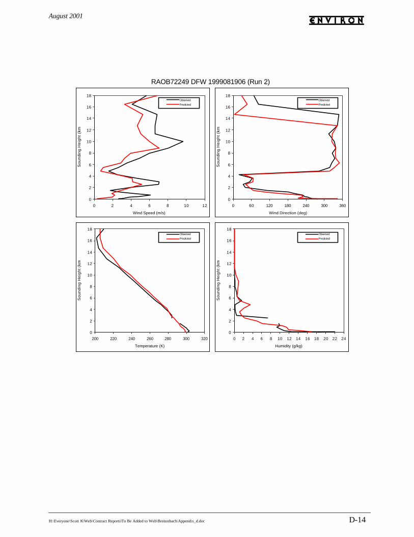
August 2001


RAOB72249 DFW 1999081906 (Run 2)

0

2

4

6

8

10

12

14

16

18

0 2 4 6 8 10 12

Wind Speed (m/s)

So

un

din

g H

eig

ht

(km

)

Observed

Predicted

0

2

4

6

8

10

12

14

16

18

0 60 120 180 240 300 360


ou

nd

ing

He

igh

t (k

m)

Observed

Predicted

0

2

4

6

8

10

12

14

16

18

200 220 240 260 280 300 320

Temperature (K)

So

un

din

g H

eig

ht

(km

)

Observed

Predicted

0

2

4

6

8

10

12

14

16

18

0 2 4 6 8 10 12 14 16 18 20 22 24

Humidity (g/kg)

So

un

din

g H

eig

ht

(km

)

Observed

Predicted

August 2001


RAOB72249 DFW 1999081918 (Run 2)

0

2

4

6

8

10

12

14

16

18

0 2 4 6 8 10

Wind Speed (m/s)

So

un

din

g H

eig

ht

(km

)

Observed

Predicted

0

2

4

6

8

10

12

14

16

18

0 60 120 180 240 300 360


So

un

din

g H

eig

ht

(km

)

Observed

Predicted

0

2

4

6

8

10

12

14

16

18

200 220 240 260 280 300 320

Temperature (K)

So

un

din

g H

eig

ht

(km

)

Observed

Predicted

0

2

4

6

8

10

12

14

16

18

0 2 4 6 8 10 12 14 16

Humidity (g/kg)

So

un

din

g H

eig

ht

(km

)

Observed

Predicted

August 2001


RAOB72249 DFW 1999082006 (Run 2)

0

2

4

6

8

10

12

14

16

18

0 2 4 6 8 10 12 14

Wind Speed (m/s)

So

un

din

g H

eig

ht

(km

)

Observed

Predicted

0

2

4

6

8

10

12

14

16

18

0 60 120 180 240 300 360


So

un

din

g H

eig

ht

(km

)

Observed

Predicted

0

2

4

6

8

10

12

14

16

18

200 220 240 260 280 300 320

Temperature (K)

So

un

din

g H

eig

ht

(km

)

Observed

Predicted

0

2

4

6

8

10

12

14

16

18

0 2 4 6 8 10 12 14 16 18

Humidity (g/kg)

So

un

din

g H

eig

ht

(km

)

Observed

Predicted

August 2001


RAOB72249 DFW 1999082018 (Run 2)

0

2

4

6

8

10

12

14

16

18

0 2 4 6 8 10 12

Wind Speed (m/s)

So

un

din

g H

eig

ht

(km

)

Observed

Predicted

0

2

4

6

8

10

12

14

16

18

0 60 120 180 240 300 360


ou

nd

ing

He

igh

t (k

m)

Observed

Predicted

0

2

4

6

8

10

12

14

16

18

200 220 240 260 280 300 320

Temperature (K)

So

un

din

g H

eig

ht

(km

)

Observed

Predicted

0

2

4

6

8

10

12

14

16

18

0 2 4 6 8 10 12

Humidity (g/kg)

So

un

din

g H

eig

ht

(km

)

Observed

Predicted

August 2001


RAOB72249 DFW 1999082106 (Run 2)

0

2

4

6

8

10

12

14

16

18

0 2 4 6 8 10 12

Wind Speed (m/s)

So

un

din

g H

eig

ht

(km

)

Observed

Predicted

0

2

4

6

8

10

12

14

16

18

0 60 120 180 240 300 360


ou

nd

ing

He

igh

t (k

m)

Observed

Predicted

0

2

4

6

8

10

12

14

16

18

200 220 240 260 280 300 320

Temperature (K)

So

un

din

g H

eig

ht

(km

)

Observed

Predicted

0

2

4

6

8

10

12

14

16

18

0 2 4 6 8 10 12 14

Humidity (g/kg)

So

un

din

g H

eig

ht

(km

)

Observed

Predicted

August 2001


RAOB72249 DFW 1999082118 (Run 2)

0

2

4

6

8

10

12

14

16

18

0 2 4 6 8 10 12 14 16 18

Wind Speed (m/s)

So

un

din

g H

eig

ht

(km

)

Observed

Predicted

0

2

4

6

8

10

12

14

16

18

0 60 120 180 240 300 360


ou

nd

ing

He

igh

t (k

m)

Observed

Predicted

0

2

4

6

8

10

12

14

16

18

200 220 240 260 280 300 320

Temperature (K)

So

un

din

g H

eig

ht

(km

)

Observed

Predicted

0

2

4

6

8

10

12

14

16

18

0 2 4 6 8 10 12 14

Humidity (g/kg)

So

un

din

g H

eig

ht

(km

)

Observed

Predicted

August 2001


RAOB72249 DFW 1999082206 (Run 2)

0

2

4

6

8

10

12

14

16

18

0 2 4 6 8 10 12

Wind Speed (m/s)

So

un

din

g H

eig

ht

(km

)

Observed

Predicted

0

2

4

6

8

10

12

14

16

18

0 60 120 180 240 300 360


So

un

din

g H

eig

ht

(km

)

Observed

Predicted

0

2

4

6

8

10

12

14

16

18

200 220 240 260 280 300 320

Temperature (K)

So

un

din

g H

eig

ht

(km

)

Observed

Predicted

0

2

4

6

8

10

12

14

16

18

0 2 4 6 8 10 12 14 16

Humidity (g/kg)

So

un

din

g H

eig

ht

(km

)

Observed

Predicted

August 2001


RAOB72249 DFW 1999081306 (Run 2)

0

2

4

6

8

10

12

14

16

18

0 2 4 6 8 10 12 14 16

Wind Speed (m/s)

So

un

din

g H

eig

ht

(km

)

Observed

Predicted

0

2

4

6

8

10

12

14

16

18

0 60 120 180 240 300 360


So

un

din

g H

eig

ht

(km

)

Observed

Predicted

0

2

4

6

8

10

12

14

16

18

200 220 240 260 280 300 320

Temperature (K)

So

un

din

g H

eig

ht

(km

)

Observed

Predicted

0

2

4

6

8

10

12

14

16

18

0 2 4 6 8 10 12 14 16 18 20 22

Humidity (g/kg)

So

un

din

g H

eig

ht

(km

)

Observed

Predicted

August 2001


September 13-20, 1999: Lake Charles 12-hourly Soundings

RAOB72240 LCHLS 1999091306 (Run 2)

0

2

4

6

8

10

12

14

16

18

0 2 4 6 8 10 12 14 16 18

Wind Speed (m/s)

So

un

din

g H

eig

ht

(km

)

Observed

Predicted

0

2

4

6

8

10

12

14

16

18

0 60 120 180 240 300 360


ou

nd

ing

He

igh

t (k

m)

Observed

Predicted

0

2

4

6

8

10

12

14

16

18

200 220 240 260 280 300 320

Temperature (K)

So

un

din

g H

eig

ht

(km

)

Observed

Predicted

0

2

4

6

8

10

12

14

16

18

0 2 4 6 8 10 12 14 16 18 20

Humidity (g/kg)

So

un

din

g H

eig

ht

(km

)

Observed

Predicted

August 2001


RAOB72240 LCHLS 1999091318 (Run 2)

0

2

4

6

8

10

12

14

16

18

0 2 4 6 8 10 12 14 16 18

Wind Speed (m/s)

So

un

din

g H

eig

ht

(km

)

Observed

Predicted

0

2

4

6

8

10

12

14

16

18

0 60 120 180 240 300 360


So

un

din

g H

eig

ht

(km

)

Observed

Predicted

0

2

4

6

8

10

12

14

16

18

200 220 240 260 280 300 320

Temperature (K)

So

un

din

g H

eig

ht

(km

)

Observed

Predicted

0

2

4

6

8

10

12

14

16

18

0 2 4 6 8 10 12 14 16 18

Humidity (g/kg)

So

un

din

g H

eig

ht

(km

)

Observed

Predicted

August 2001


RAOB72240 LCHLS 1999091406 (Run 2)

0

2

4

6

8

10

12

14

16

18

0 2 4 6 8 10 12 14 16 18 20 22

Wind Speed (m/s)

So

un

din

g H

eig

ht

(km

)

Observed

Predicted

0

2

4

6

8

10

12

14

16

18

0 60 120 180 240 300 360


ou

nd

ing

He

igh

t (k

m)

Observed

Predicted

0

2

4

6

8

10

12

14

16

18

200 220 240 260 280 300 320

Temperature (K)

So

un

din

g H

eig

ht

(km

)

Observed

Predicted

0

2

4

6

8

10

12

14

16

18

0 2 4 6 8 10 12 14 16

Humidity (g/kg)

So

un

din

g H

eig

ht

(km

)

Observed

Predicted

August 2001


RAOB72240 LCHLS 1999091418 (Run 2)

0

2

4

6

8

10

12

14

16

18

0 2 4 6 8 10 12 14 16 18 20 22

Wind Speed (m/s)

So

un

din

g H

eig

ht

(km

)

Observed

Predicted

0

2

4

6

8

10

12

14

16

18

0 60 120 180 240 300 360


So

un

din

g H

eig

ht

(km

)

Observed

Predicted

0

2

4

6

8

10

12

14

16

18

200 220 240 260 280 300 320

Temperature (K)

So

un

din

g H

eig

ht

(km

)

Observed

Predicted

0

2

4

6

8

10

12

14

16

18

0 2 4 6 8 10 12 14

Humidity (g/kg)

So

un

din

g H

eig

ht

(km

)

Observed

Predicted

August 2001


RAOB72240 LCHLS 1999091506 (Run 2)

0

2

4

6

8

10

12

14

16

18

0 2 4 6 8 10 12 14 16 18 20 22 24

Wind Speed (m/s)

So

un

din

g H

eig

ht

(km

)

Observed

Predicted

0

2

4

6

8

10

12

14

16

18

0 60 120 180 240 300 360


So

un

din

g H

eig

ht

(km

)

Observed

Predicted

0

2

4

6

8

10

12

14

16

18

200 220 240 260 280 300 320

Temperature (K)

So

un

din

g H

eig

ht

(km

)

Observed

Predicted

0

2

4

6

8

10

12

14

16

18

0 2 4 6 8 10 12

Humidity (g/kg)

So

un

din

g H

eig

ht

(km

)

Observed

Predicted

August 2001


RAOB72240 LCHLS 1999091606 (Run 2)

0

2

4

6

8

10

12

14

16

18

0 2 4 6 8 10 12 14 16 18 20

Wind Speed (m/s)

So

un

din

g H

eig

ht

(km

)

Observed

Predicted

0

2

4

6

8

10

12

14

16

18

0 60 120 180 240 300 360


ou

nd

ing

He

igh

t (k

m)

Observed

Predicted

0

2

4

6

8

10

12

14

16

18

200 220 240 260 280 300 320

Temperature (K)

So

un

din

g H

eig

ht

(km

)

Observed

Predicted

0

2

4

6

8

10

12

14

16

18

0 2 4 6 8 10 12

Humidity (g/kg)

So

un

din

g H

eig

ht

(km

)

Observed

Predicted

August 2001


RAOB72240 LCHLS 1999091618 (Run 2)

0

2

4

6

8

10

12

14

16

18

0 2 4 6 8 10 12 14 16 18 20 22

Wind Speed (m/s)

So

un

din

g H

eig

ht

(km

)

Observed

Predicted

0

2

4

6

8

10

12

14

16

18

0 60 120 180 240 300 360


So

un

din

g H

eig

ht

(km

)

Observed

Predicted

0

2

4

6

8

10

12

14

16

18

200 220 240 260 280 300 320

Temperature (K)

So

un

din

g H

eig

ht

(km

)

Observed

Predicted

0

2

4

6

8

10

12

14

16

18

0 2 4 6 8 10 12

Humidity (g/kg)

So

un

din

g H

eig

ht

(km

)Observed

Predicted

August 2001


RAOB72240 LCHLS 1999091706 (Run 2)

0

2

4

6

8

10

12

14

16

18

0 2 4 6 8 10 12 14 16 18 20 22 24 26

Wind Speed (m/s)

So

un

din

g H

eig

ht

(km

)

Observed

Predicted

0

2

4

6

8

10

12

14

16

18

0 60 120 180 240 300 360


So

un

din

g H

eig

ht

(km

)

Observed

Predicted

0

2

4

6

8

10

12

14

16

18

200 220 240 260 280 300

Temperature (K)

So

un

din

g H

eig

ht

(km

)

Observed

Predicted

0

2

4

6

8

10

12

14

16

18

0 2 4 6 8 10 12

Humidity (g/kg)

So

un

din

g H

eig

ht

(km

)

Observed

Predicted

August 2001


RAOB72240 LCHLS 1999091718 (Run 2)

0

2

4

6

8

10

12

14

16

18

0 2 4 6 8 10 12 14 16 18 20 22 24 26

Wind Speed (m/s)

So

un

din

g H

eig

ht

(km

)

Observed

Predicted

0

2

4

6

8

10

12

14

16

18

0 60 120 180 240 300 360


So

un

din

g H

eig

ht

(km

)

Observed

Predicted

0

2

4

6

8

10

12

14

16

18

200 220 240 260 280 300 320

Temperature (K)

So

un

din

g H

eig

ht

(km

)

Observed

Predicted

0

2

4

6

8

10

12

14

16

18

0 2 4 6 8 10 12

Humidity (g/kg)

So

un

din

g H

eig

ht

(km

)

Observed

Predicted

August 2001


RAOB72240 LCHLS 1999091806 (Run 2)

0

2

4

6

8

10

12

14

16

18

0 2 4 6 8 10 12 14 16 18 20 22 24 26 28

Wind Speed (m/s)

So

un

din

g H

eig

ht

(km

)

Observed

Predicted

0

2

4

6

8

10

12

14

16

18

0 60 120 180 240 300 360


So

un

din

g H

eig

ht

(km

)

Observed

Predicted

0

2

4

6

8

10

12

14

16

18

200 220 240 260 280 300 320

Temperature (K)

So

un

din

g H

eig

ht

(km

)

Observed

Predicted

0

2

4

6

8

10

12

14

16

18

0 2 4 6 8 10 12

Humidity (g/kg)

So

un

din

g H

eig

ht

(km

)Observed

Predicted

August 2001


RAOB72240 LCHLS 1999091818 (Run 2)

0

2

4

6

8

10

12

14

16

18

0 2 4 6 8 10 12 14 16 18 20 22 24 26 28 30

Wind Speed (m/s)

So

un

din

g H

eig

ht

(km

)

Observed

Predicted

0

2

4

6

8

10

12

14

16

18

0 60 120 180 240 300 360


ou

nd

ing

He

igh

t (k

m)

Observed

Predicted

0

2

4

6

8

10

12

14

16

18

200 220 240 260 280 300 320

Temperature (K)

So

un

din

g H

eig

ht

(km

)

Observed

Predicted

0

2

4

6

8

10

12

14

16

18

0 2 4 6 8 10 12

Humidity (g/kg)

So

un

din

g H

eig

ht

(km

)

Observed

Predicted

August 2001


RAOB72240 LCHLS 1999091906 (Run 2)

0

2

4

6

8

10

12

14

16

18

0 2 4 6 8 10 12 14 16 18 20 22 24 26 28 30

Wind Speed (m/s)

So

un

din

g H

eig

ht

(km

)

Observed

Predicted

0

2

4

6

8

10

12

14

16

18

0 60 120 180 240 300 360


So

un

din

g H

eig

ht

(km

)

Observed

Predicted

0

2

4

6

8

10

12

14

16

18

200 220 240 260 280 300 320

Temperature (K)

So

un

din

g H

eig

ht

(km

)

Observed

Predicted

0

2

4

6

8

10

12

14

16

18

0 2 4 6 8 10 12 14

Humidity (g/kg)

So

un

din

g H

eig

ht

(km

)

Observed

Predicted

August 2001


RAOB72240 LCHLS 1999091918 (Run 2)

0

2

4

6

8

10

12

14

16

18

0 2 4 6 8 10 12 14 16 18 20 22 24 26

Wind Speed (m/s)

So

un

din

g H

eig

ht

(km

)

Observed

Predicted

0

2

4

6

8

10

12

14

16

18

0 60 120 180 240 300 360


So

un

din

g H

eig

ht

(km

)

Observed

Predicted

0

2

4

6

8

10

12

14

16

18

200 220 240 260 280 300 320

Temperature (K)

So

un

din

g H

eig

ht

(km

)

Observed

Predicted

0

2

4

6

8

10

12

14

16

18

0 2 4 6 8 10 12

Humidity (g/kg)

So

un

din

g H

eig

ht

(km

)

Observed

Predicted

August 2001


RAOB72240 LCHLS 1999092006 (Run 2)

0

2

4

6

8

10

12

14

16

18

0 2 4 6 8 10 12 14 16 18 20 22 24 26 28 30

Wind Speed (m/s)

So

un

din

g H

eig

ht

(km

)

Observed

Predicted

0

2

4

6

8

10

12

14

16

18

0 60 120 180 240 300 360


ou

nd

ing

He

igh

t (k

m)

Observed

Predicted

0

2

4

6

8

10

12

14

16

18

200 220 240 260 280 300 320

Temperature (K)

So

un

din

g H

eig

ht

(km

)

Observed

Predicted

0

2

4

6

8

10

12

14

16

18

0 2 4 6 8 10 12 14 16

Humidity (g/kg)

So

un

din

g H

eig

ht

(km

)

Observed

Predicted

August 2001


RAOB72240 LCHLS 1999092018 (Run 2)

0

2

4

6

8

10

12

14

16

18

0 2 4 6 8 10 12 14 16 18 20 22 24 26 28 30

Wind Speed (m/s)

So

un

din

g H

eig

ht

(km

)Observed

Predicted

0

2

4

6

8

10

12

14

16

18

0 60 120 180 240 300 360


So

un

din

g H

eig

ht

(km

)

Observed

Predicted

0

2

4

6

8

10

12

14

16

18

200 220 240 260 280 300 320

Temperature (K)

So

un

din

g H

eig

ht

(km

)

Observed

Predicted

0

2

4

6

8

10

12

14

16

18

0 2 4 6 8 10 12 14 16

Humidity (g/kg)

So

un

din

g H

eig

ht

(km

)

Observed

Predicted

international corporation air sciences€¦ · · 2001-09-07international corporation air...

Documents