International Capital Flows1

Cédric Tille

Graduate Institute of International and Development Studies, Geneva

CEPR

Eric van Wincoop

University of Virginia

NBER

August 19, 2008

1Cédric Tille: Graduate Institute of International and Development Studies, Pavil-

lon Rigot, Avenue de la Paix 11A, 1202 Geneva, Switzerland, Phone +41 22 908 5928,

Fax +41 22 733 3049, cedric.tille@graduateinstitute.ch. Eric van Wincoop: Department

of Economics, University of Virginia, 2015 Ivy Road Charlottesville, VA 22904, van-

wincoop@virginia.edu. We thank seminar participants at the 2008 Annual meeting of

the American Economic Association, the NBER IFM meeting, the Board of Governors,

the IMF, the Second Annual Conference on Macroeconomics of Global Interdependence

in Dublin, the Federal Reserve Bank of New York, Georgetown University, the Gradu-

ate Institute of International Studies, the Hong Kong Institute for Monetary Research,

Hong Kong University, the Hong Kong University of Science and Technology, Harvard,

Cornell, NYU, the University of Connecticut and Wharton for comments. We also

thank Philippe Bacchetta, Pierpaolo Benigno, Mick Devereux, Martin Evans, Viktoria

Hnatkovska, Robert Kollmann, Enrique Mendoza, Asaf Razin, Alan Sutherland, Jaume

Ventura and Frank Warnock for comments and discussions. van Wincoop acknowledges

�nancial support from the Hong Kong Institute for Monetary Research, the Bankard

Fund for Political Economy and the National Science Foundation (grant SES-0649442).

Abstract

The surge in international asset trade since the early 1990s has lead to renewed

interest in models with international portfolio choice. We develop the implications

of portfolio choice for both gross and net international capital �ows in the context of

a simple two-country dynamic stochastic general equilibrium (DSGE) model. We

focus on the time-variation in portfolio allocation following shocks, and resulting

capital �ows. Endogenous time-variation in expected returns and risk, which are

the key determinants of portfolio choice, a¤ect capital �ows in often subtle ways.

The model is consistent with a broad range of empirical evidence. An additional

contribution of the paper is to overcome the technical di¢ culty of solving DSGE

models with portfolio choice by developing a broadly applicable solution method.

JEL classi�cation: F32, F36, F41

Keywords: international capital �ows, portfolio allocation, home bias.

1 Introduction

In his Ohlin lecture, Obstfeld (2007) emphasizes the �explosion in interna-

tional asset trade�since the early 1990s and calls for the development of a general

equilibrium portfolio-balance model to analyze its implications, echoing his earlier

statement that �at the moment we have no integrative general-equilibrium mon-

etary model of international portfolio choice, although we need one� (Obstfeld,

2004). The recent surge in international �nancial integration1 has indeed lead to a

broad consensus on the need to include portfolio choice in such models, an aspect

that has been cast aside since ad-hoc portfolio balance models of the 1970s fell out

of favor. Typical of current views, Gourinchas (2006) writes �Looking ahead, the

next obvious step is to build general equilibrium models of international portfolio

allocation with incomplete markets. I see this as a major task that will close a

much needed gap in the literature... �.

The goal of this paper is to �ll this gap. We develop the implications of portfolio

choice for both gross and net international capital �ows in the context of a simple

two-country dynamic stochastic general equilibrium (DSGE) model. We show

how endogenous time-variation in expected returns and risk, which are the key

determinants of portfolio choice, a¤ect capital �ows. We deliberately consider a

simple model to focus squarely on portfolio choice. While we do not formally test

the model, we show that it is consistent with a broad range of empirical evidence.

An additional contribution of the paper is to overcome the technical di¢ culty of

solving DSGE models with portfolio choice by developing a solution method that

is broadly applicable beyond our simple setup.

The analysis reveals some surprising results regarding the role of time-varying

risk and expected returns. First, we show that even though the variance of the

shocks in the model is held constant, the second moments that drive portfolio choice

endogenously vary in response to movements in the state space. Second, these

�uctuations in second moments a¤ect capital �ows only to the extent that they

a¤ect the portfolio choice of domestic and foreign investors di¤erently. We show

that they can be an important driving force behind international capital �ows and

generate a positive co-movement between gross capital in�ows and out�ows that

is consistent with the data. Third, while endogenous changes in the di¤erence in

expected returns across assets a¤ect portfolio choice, the link between capital �ows

1See for instance Gourinchas and Rey (2007), Lane and Milesi-Ferretti (2005) and Tille (2008).

and expected returns is weak. This is both because expected return di¤erences

are small in equilibrium and because several important factors driving expected

return di¤erences have no bearing on capital �ows. This suggests caution when

conducting empirical work on the link between capital �ows and expected returns.

The model also sheds light on the mechanisms through which international

imbalances are �nanced. The traditional view is that an external debt is �nanced

through the present value of future trade surpluses. Recently however, Gourinchas

and Rey (2007) have emphasized that it can also be �nanced through higher ex-

pected returns on external assets than liabilities, and �nd a signi�cant role for this

expected asset return channel for the United States. Our analysis con�rms that

expected asset price changes (both exchange rates and equity prices) play a role in

�nancing the external debt. Nonetheless, the income streams on the various assets

(e.g. dividends) adjust to equalize the predictable overall returns across assets

(dividends plus expected asset price changes). This implies that to a �rst-order an

external debt is fully �nanced by future trade surpluses.2

One of the main reasons that portfolio choice has been largely absent from

open economy DSGE models is the di¢ culty in solving such models. The standard

method for solving DSGE models is to simply linearize around the deterministic

steady state, and then solve the resulting set of linear di¤erence equations. This

can be extended to compute the second-order solution of the model. These methods

can be easily be implemented in large models. However, this standard approach

breaks down in the presence of portfolio choice. For example, the allocation around

which the model is expanded cannot be the deterministic steady state as portfolio

choice is undetermined in such an environment.

The solution method we develop stays very close to the familiar �rst and sec-

ond order approximation techniques. Indeed, the model is solved using them for

all equations except the optimality conditions for portfolio choice, which need to

be approximated to higher orders. Intuitively, this re�ects the fact that portfolio

allocation is about risk, a dimension that is not captured by a �rst-order approx-

imation. Speci�cally, solving for portfolio choice in the allocation around which

the model is expanded requires a second-order expansion of optimality conditions

for portfolio choice in order to capture the risk at the core of portfolio choice. In

order to capture the time-variation of portfolio allocation a third-order expansion

2Pavlova and Rigobon (2007) independently develop a similar point.

of the optimality conditions for portfolio choice is needed. While third-order terms

are usually seen as irrelevant due to their small magnitude, this is not the case in

the context of portfolio choice where third-order changes in expected returns and

risk induce �rst-order changes in portfolio shares.3 An important point is that the

method is not limited to the simple model that we consider, but is applicable to a

broad range of richer settings.

The remainder of the paper is organized as follows. Section 2 puts our work

in the context related literature on the role of portfolio choice. Our simple model

is described in Section 3, with Section 4 discussing the solution method. We

develop various implications for international capital �ows in Section 5. Section 6

illustrates our results using a numerical example and relates various implications

of the model to a broad range of empirical evidence. Section 7 concludes.

2 Related Literature

Portfolio balance models of the late 1970s and early 1980s modeled asset de-

mand as a function of expected asset returns, income, wealth and prices. A nice

review can be found in Branson and Henderson (1985). A clear drawback of this

literature is that asset demand speci�cations were not derived from optimization.

A number of papers at the time did consider the micro foundations of asset demand

in the context of open economy models with optimal portfolio choice.4 However,

these were partial equilibrium models and the portfolio choice elements were never

fully integrated in the general equilibrium models that followed.

Since the early 1980s these models were gradually replaced by general equilib-

rium models with optimizing agents. Portfolio choice was overlooked as most of

these models assume that either only a riskfree bond is traded or that �nancial

markets are complete. The one-asset models have nothing to say about gross inter-

national capital �ows or asset positions. This is a problem because asset trade, just

3For example, in a simple two-asset portfolio choice problem portfolio shares will depend

on the expected excess return (the di¤erence in return between the two assets) divided by the

variance of the excess return. Since the denominator (variance of excess return) is second-order,

a third-order change in the expected excess return leads to a �rst-order change in the portfolio

share.4See for example Adler and Dumas (1983), Braga de Macedo (1983), Braga de Macedo,

Goldstein and Meerschwam (1984), Kouri (1976), Kouri and Braga de Macedo (1978) and the

review in Branson and Henderson (1985).

like goods trade, is two-way trade with similar assets (e.g. equity) both imported

and exported. Moreover, changes in expected returns in one country relative to

another, or changes in risk characteristics of assets, play no role. At the other

extreme, in models where �nancial markets are complete, Obstfeld and Rogo¤

(1996) argue that capital �ows are �...merely an accounting device for tracking the

international distribution of new equity claims foreigners must buy to maintain

the e¢ cient global pooling of national output risks.�Capital �ows are rarely even

considered in these models as the real allocation can be computed independent of

the exact structure of asset markets that implements asset market completeness.5

Portfolio choice was not completely cast aside, as a large and still growing

literature has considered the issue of portfolio home bias. However, this liter-

ature is concerned with the steady state portfolio allocation rather than with

time-variation in portfolio allocation that gives rise to capital �ows. Some re-

cent contributions along this line include Engel and Matsumoto (2006), Heathcote

and Perri (2007), Kollman (2006), Coeurdacier (2007) and Coeurdacier, Kollmann

and Martin (2007).

The impact of portfolio choice on capital �ows was analyzed explicitly in the

important contributions by Kraay and Ventura (2000,2003). While they consider

partial equilibrium small open economy models, with an exogenous return on in-

vestment abroad and only one-way capital �ows (from the small to the large coun-

try), these papers are nonetheless important as they are the �rst ones to develop

a portfolio perspective on international capital �ows. They make a key distinction

between portfolio growth (investment of saving at steady state portfolio shares)

and portfolio reallocation (change in optimal portfolio shares), which we will adopt

here as well.

In terms of the solution method the paper is most closely related to Dev-

ereux and Sutherland (2007). They independently and simultaneously developed

a solution method for DSGE models with portfolio choice that is essentially the

same as ours, as discussed in Section 4.6 Their contribution focuses only on the

methodological aspects though and does not discuss implications for international

capital �ows. The work by Evans and Hnatkovska (2007b) is important as well.

Their method combines a variety of discrete time approaches (perturbation and

5In a setup where a full set of Arrow Debreu securities covering all possible future contingencies

is traded in an initial period, subsequent capital �ows will simply be zero.6Their work builds on the previous papers Devereux and Sutherland (2006, 2008).

projection methods) with continuous time approximations (of portfolio return and

second-order dynamics of the state variables), making it hard to compare to the

one developed here.7 By contrast, our method stays closer to standard �rst and

second-order solution methods.

Most recently Rigobon and Pavlova (2007) develop an analytical solution to

a DSGE model with portfolio choice and discuss various issues associated with

external debt �nancing. The model and solution method are elegant, but analytical

solutions can only be achieved for particular parameterizations (e.g. log utility).

The same can also be said of Devereux and Saito (2007), who also derive an

analytical solution for portfolio choice in a DSGE model. The focus in that paper

is on the stationarity of the international wealth distribution.

3 A two-country, two-good, two-asset model

We consider a deliberately minimalist model that focuses squarely on the op-

timal international allocation of portfolios and abstracts from all other decisions.

Our approach adopts almost the exact opposite modeling strategy as in stan-

dard DSGE open economy models, which encompass decisions about consumption,

leisure and investment, but ignore portfolio choice. Our choice of a simple setup is

solely to focus on the key element that has been missing from dynamic stochastic

open economy models. As we will discuss later, the solution method can easily be

applied to richer and more complex models.

3.1 Two goods: production and consumption

There are two countries of equal size, Home and Foreign, that each produce a

di¤erent good that is consumed worldwide. Production uses a constant returns to

scale technology combining labor and capital:

Yi;t = Ai;tK1��i;t N �

i;t i = H;F

whereH and F denote the Home and Foreign country respectively. Yi is the output

of the country i good, Ki is the capital input and Ni the labor input. Ai is an

7Evans and Hnatkovska (2005, 2007a) and Hnatkovska (2006) apply the solution method to

discuss implications for issues such as the volatility of asset prices, the implications of interna-

tional �nancial integration and portfolio home bias.

exogenous stochastic productivity term which is the only source of shocks in the

model. A share � of output is paid to labor, with the remaining going to capital.

The capital stocks and labor inputs are �xed and normalized to unity. Outputs

therefore simply re�ect the levels of productivity, which follow an exogenous auto-

regressive process:

Yi;t = Ai;t ; ai;t+1 = �ai;t + �i;t+1 (1)

where lower case letters denote logs and � 2 (0; 1). The productivity innovationsin both countries are iid, with a N(0; �2) distribution.

We consider home bias in preferences, with consumers putting a higher weight

on locally-produced goods. The resulting di¤erence in the consumption baskets

and consumer prices generate a role for movements in the real exchange rate. The

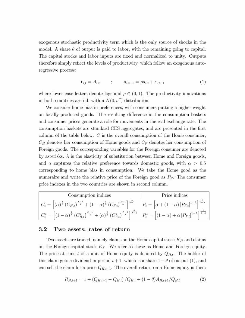
consumption baskets are standard CES aggregates, and are presented in the �rst

column of the table below. C is the overall consumption of the Home consumer,

CH denotes her consumption of Home goods and CF denotes her consumption of

Foreign goods. The corresponding variables for the Foreign consumer are denoted

by asterisks. � is the elasticity of substitution between Home and Foreign goods,

and � captures the relative preference towards domestic goods, with � > 0:5

corresponding to home bias in consumption. We take the Home good as the

numeraire and write the relative price of the Foreign good as PF . The consumer

price indexes in the two countries are shown in second column.

Consumption indices Price indices

Ct =h(�)

1� (CH;t)

��1� + (1� �)

1� (CF;t)

��1�

i ���1

Pt =h�+ (1� �) [PF;t]

1��i 11��

C�t =h(1� �)

1��C�H;t

���1� + (�)

1��C�F;t

���1�

i ���1

P �t =h(1� �) + � [PF;t]

1��i 11��

3.2 Two assets: rates of return

Two assets are traded, namely claims on the Home capital stockKH and claims

on the Foreign capital stock KF . We refer to these as Home and Foreign equity.

The price at time t of a unit of Home equity is denoted by QH;t. The holder of

this claim gets a dividend in period t+1, which is a share 1� � of output (1), andcan sell the claim for a price QH;t+1. The overall return on a Home equity is then:

RH;t+1 = 1 + (QH;t+1 �QH;t) =QH;t + (1� �)AH;t+1=QH;t (2)

Similarly, the price at time t of a unit of Foreign equity is denoted by QF;t, and

the return on Foreign equity is:

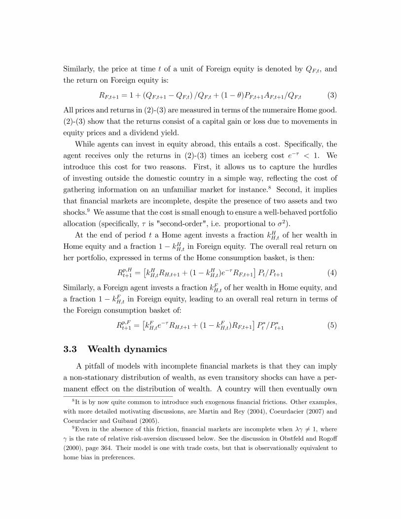
RF;t+1 = 1 + (QF;t+1 �QF;t) =QF;t + (1� �)PF;t+1AF;t+1=QF;t (3)

All prices and returns in (2)-(3) are measured in terms of the numeraire Home good.

(2)-(3) show that the returns consist of a capital gain or loss due to movements in

equity prices and a dividend yield.

While agents can invest in equity abroad, this entails a cost. Speci�cally, the

agent receives only the returns in (2)-(3) times an iceberg cost e�� < 1. We

introduce this cost for two reasons. First, it allows us to capture the hurdles

of investing outside the domestic country in a simple way, re�ecting the cost of

gathering information on an unfamiliar market for instance.8 Second, it implies

that �nancial markets are incomplete, despite the presence of two assets and two

shocks.9 We assume that the cost is small enough to ensure a well-behaved portfolio

allocation (speci�cally, � is "second-order", i.e. proportional to �2).

At the end of period t a Home agent invests a fraction kHH;t of her wealth in

Home equity and a fraction 1� kHH;t in Foreign equity. The overall real return on

her portfolio, expressed in terms of the Home consumption basket, is then:

Rp;Ht+1 =�kHH;tRH;t+1 + (1� kHH;t)e

��RF;t+1�Pt=Pt+1 (4)

Similarly, a Foreign agent invests a fraction kFH;t of her wealth in Home equity, and

a fraction 1 � kFH;t in Foreign equity, leading to an overall real return in terms of

the Foreign consumption basket of:

Rp;Ft+1 =�kFH;te

��RH;t+1 + (1� kFH;t)RF;t+1�P �t =P

�t+1 (5)

3.3 Wealth dynamics

A pitfall of models with incomplete �nancial markets is that they can imply

a non-stationary distribution of wealth, as even transitory shocks can have a per-

manent e¤ect on the distribution of wealth. A country will then eventually own8It is by now quite common to introduce such exogenous �nancial frictions. Other examples,

with more detailed motivating discussions, are Martin and Rey (2004), Coeurdacier (2007) and

Coeurdacier and Guibaud (2005).9Even in the absence of this friction, �nancial markets are incomplete when � 6= 1, where

is the rate of relative risk-aversion discussed below. See the discussion in Obstfeld and Rogo¤

(2000), page 364. Their model is one with trade costs, but that is observationally equivalent to

home bias in preferences.

the entire world, so that the long run wealth distribution is not determined. This

indeterminacy rules out the use of the standard approximation methods as there

is no allocation to which the economy will converge.

We get around this problem by considering investors with �nite lives, following

the framework of Caballero, Fahri and Gourinchas (2008). Speci�cally, agents die

with constant probability each period, and new agents are born at the same rate

to keep the population constant. Keeping with our focus on portfolio choice, we

abstract from any other decision. Newborn agents inelastically supply one unit

of labor and never work thereafter. Dying agents liquidate their entire wealth

and consume. The other agents re-invest their wealth in the two equities, possibly

altering their portfolio allocation. This is their only decision. Since the probability

of death is the same for all agents, total consumption is simply equal to aggregate

wealth times the probability of death.

The wealth of a particular Home investor j accumulates according to

W jt+1 = W j

t Rp;Ht+1 (6)

where Rp;Ht+1 is given by (4).10 Aggregate wealth accumulation di¤ers from (6) for

three reasons. First, only the agents that will be alive next period participate in

asset markets. They account for a fraction 1 � of wealth. Second, the labor

income of the newborns raises aggregate wealth. Third, the cost of investment

abroad, � , does not a¤ect the dynamics of aggregate wealth. Speci�cally, we

assume that it does not represent lost resources, but instead is a fee paid to a broker,

which we take to be the newborn agents. We denote the aggregate wealth of the

Home and Foreign countries, measured in terms of their respective consumption

baskets, by Wt and W �t . Their dynamics are given by:

Wt+1 = (1� )�kHH;tRH;t+1 + (1� kHH;t)RF;t+1

� PtPt+1

Wt +�AH;t+1Pt+1

(7)

W �t+1 = (1� )

�kFH;tRH;t+1 + (1� kFH;t)RF;t+1

� P �tP �t+1

W �t +

�PF;t+1AF;t+1P �t+1

(8)

10The portfolio return will be the same for all Home investors as they all choose the same

portfolio in equilibrium.

3.4 Markets clearing

Using (1) and the allocation of consumption between Home and Foreign goods,

the two goods market clearing conditions are

AH;t = � (Pt)� Wt + (1� �) (P �t )

� W �t (9)

AF;t = (1� �) (PF;t)�� (Pt)

� Wt + � (PF;t)�� (P �t )

� W �t (10)

Turning to asset markets, the total values of Home and Foreign equity supply

are equal to QH;t and QF;t since the capital stocks are normalized to 1. The

amounts invested by Home and Foreign agents at the end of period t, measured in

Home goods, are (1� )WtPt and (1� )W �t P

�t respectively. The market clearing

conditions for Home and Foreign asset markets are then

QH;t = (1� )�kHH;tWtPt + kFH;tW

�t P

�t

�(11)

QF;t = (1� )�(1� kHH;t)WtPt + (1� kFH;t)W

�t P

�t

�(12)

3.5 Portfolio allocation

The only decision faced by agents is the allocation of their investment between

Home and Foreign equity. A Home agent j who dies in period t+ 1 consumes her

entire wealth and gets utility

U jt+1 =�W jt+1

�1� =(1� ) > 1

We denote the value of wealth in period t by V (W jt ). As agents face a probability

of dying the next period, the Bellman equation is

V (W jt ) = �(1� )EtV (W

jt+1) + � Et

�W jt+1

�1� =(1� ) (13)

where � is the discount rate.

We conjecture the following form for the value of wealth:

V (W jt ) = ev+fH(St)

�W jt

�1� =(1� ) (14)

where v is a constant, St is the state space discussed below and the function

fH(St) captures time variation in expected portfolio returns, which endogenously

vary with the state. For given wealth, utility is higher (fH(St) is lower) the larger

are expected future portfolio returns. For Foreign investors the function fH(St) is

replaced by fF (St).

Agent j of the Home country chooses the portfolio allocation to maximize (13),

subject to (6) and (4). The �rst-order conditions for Home and Foreign investors

are:

Et�t�RH;t+1 � e��RF;t+1

�= 0 ; Et�

�t

�e��RH;t+1 �RF;t+1

�= 0 (15)

where

�t =�(1� )ev+fH(St+1) +

� �Rp;Ht+1

�� Pt=Pt+1

��t =�(1� )ev+fF (St+1) +

� �Rp;Ft+1

�� P �t =P

�t+1

are the asset pricing kernels of the Home and Foreign investors respectively. The

optimality conditions for portfolio choice (15) show that investors equalize the

expected discounted return on each asset. Therefore the expected product of the

asset pricing kernel and the excess return is equal to zero.

Using (14), the Bellman equation (13) for a representative investor in country

i is

ev+fi(St) = �Et�(1� )ev+fi(St+1) +

� �Rp;it+1

�1� i = H;F (16)

which gives an implicit solution to the function fi(St).

4 Solution of the model

The model consists of 11 independent equations that are listed in Appendix A.

The solution method is made clearer by de�ning two measures of portfolio shares.

The average share invested in Home equity is denoted by kAt = 0:5(kHH;t + kFH;t).

The di¤erence in portfolio shares captures the extent to which Home investors are

more heavily invested in Home equity than Foreign investors are, and is written

as kDt = kHH;t � kFH;t. It is therefore a measure of portfolio home bias.

The solution method builds on standard linear and quadratic approximation

methods around an allocation. While this allocation is usually computed as the

deterministic steady state, the introduction of portfolio choice raises a complex-

ity. As portfolio choice is driven by risk, it is not well-de�ned in a deterministic

environment. The problem arises speci�cally for the di¤erence across countries in

portfolio shares. Even in a deterministic environment, the average portfolio share,

kAt , is simply determined by the asset market clearing conditions (11)-(12). These

conditions show how much Home and Foreign equity needs to be held by investors

in equilibrium, but shed no light on which investor should hold it. The di¤erence

in portfolio shares, kDt , is not well-de�ned in a deterministic equilibrium. The so-

lution method therefore gives special treatment to the di¤erence in portfolio shares

and the di¤erence in portfolio Euler equations (15) between Home and the Foreign

investors. No special treatment is required for any of the remaining equations and

variables, which we refer to as the �other equations� and �other variables� for

brevity. As discussed above, the average portfolio share, kAt , is one of these �other

variables�.

A central aspect of our approach is to split the various variables across compo-

nents of di¤erent orders. A variable xt can be written as the sum of its zero-order,

�rst-order and higher-order components, namely: xt = x(0) + xt(1) + xt(2) + :::.

The zero-order component, x(0), is the value of xt when the volatility of shocks be-

comes arbitrarily small (� ! 0). The �rst-order component, xt(1), is proportional

to � or model innovations. The second-order component, xt(2), is proportional

to �2 or the product of model innovations, and so on. This decomposition also

applies to portfolio shares, and in particular to the di¤erence kDt . For instance, the

zero-order portfolio di¤erence, kD (0), is independent of the value of �, as shown

below. Note that it is only de�ned as long as � is positive, even if in�nitesimally

small.

In order to compute �rst and higher-order components of model equations we

expand around zero-order components of all variables. The zero-order compo-

nents of the �other variables� follow directly from the zero-order components of

the �other equations�.11 Computing the zero-order component of the di¤erence in

portfolio shares is more complex. We now turn to the description of the solution

method, which proceeds in two steps. We keep the description as non-technical as

possible, focusing on the methodology. The technical details are outlined in Ap-

pendices B and C for the �rst and second-order components of Bellman equations

and the third-order components of Euler equations for portfolio choice, with a full

11In particular, dropping country subscripts due to symmetry, we have W (0) = 1= , R(0) =

(1� �) = (1� ), Q(0) = (1� ) = , A(0) = PF (0) = 1, v(0) = ln( )� ln(R(0) �1=� � 1 + )and kA(0) = 0:5.

description of all the algebra left to a Technical Appendix available on request.12

4.1 The �rst step

The �rst step involves jointly solving the �rst-order component of the �other

variables�and the zero-order component of the di¤erence in portfolio shares kDt .

First-order solution of �other variables�

Conditional on a value for the zero-order component of the di¤erence in portfo-

lio shares, kD(0), the �rst-order component of the �other variables�is solved from

the �rst-order component of the �other equations�using the entirely standard �rst-

order solution method based on a log-linear approximation around the zero-order

values of the variables. We de�ne the di¤erence and average of variables across

countries with superscripts D and A (xDt = xHt �xFt and xAt = 0:5(xHt +xFt )). Themodel boils down to 5 control variables and 3 state variables:13

cvt = (wAt ; pF;t; kAt ; qH;t; qF;t)

0 (17)

St =�aDt ; w

Dt ; a

At

�0(18)

The standard �rst-order solution technique applied to the �rst-order components

of the log-linearized equations then provides a solution of the following form:

cvt(1) = BSt(1) ; St+1(1) = N1St(1) +N2�t+1 (19)

where B, N1 and N2 are matrices and �t+1 = (�H;t+1; �F;t+1)0 are the model in-

novations. The �rst-order component of the Bellman equations (16) gives the

�rst-order components of the functions fH(St) and fF (St), denoted by H1;HSt(1)

and H1;FSt(1), and also implies v(1) = 0.

Zero-order solution of portfolio share di¤erence

The �rst-order solution (19) is conditional on the unknown kD(0), which is

solved by taking the second-order component of the di¤erence across countries of

12In the working paper version, Tille and van Wincoop (2007), we provide a more general

description of the solution method that applies to any order of approximation.13The average wealth level is not a separate state variable as the �rst-order components of wAt

and aAt are identical.

the portfolio Euler equations (15). Abstracting from the algebraic details, we get

kD(0) = 2�

var(ert+1(1))+ � 1

cov(pt+1(1)� p�t+1(1); ert+1(1))

var(ert+1(1))(20)

+(1� 0)cov((H1;H �H1;F )St+1(1); ert+1(1))

var(ert+1(1))

where ert+1 = rH;t+1 � rF;t+1 is the excess return on Home equity, and 0 =

1 � �(1 � )R(0)1� . Each of the three terms on the right-hand side of (20) is

a ratio of second-order variables (proportional to �2). This illustrates why the

second-order components of portfolio Euler equations are necessary to compute

the zero-order component of portfolio shares.

In terms of economic intuition, a positive value of (20) implies portfolio home

bias, while a negative value implies foreign bias. (20) shows three sources of port-

folio bias. The �rst re�ects the cost of investing abroad, � , with a higher cost

making investing in domestic equity more attractive. The second re�ects the co-

movements of the real exchange rate and excess return. Assuming > 1, it is

attractive for Home investors to invest in the Home equity if the excess return on

Home equity is high in states where the Home price index is relatively high, i.e.

Home equity is a good hedge of real exchange rate risk. The �nal source re�ects

a hedge against changes in future expected portfolio returns, which are captured

by the functions H1;HSt+1(1) and H1;FSt+1(1) in the value function of Home and

Foreign investors next period. A high value of these functions indicates a future

state with low expected returns. It is attractive for Home investors to invest in

Home equity when the excess return on Home equity is high in such states.

Fixed point problem

With the exception of � , all the second-order components in the three ratios

in (20) are based on variances and covariances of �rst-order components of model

variables. These can be computed from the �rst-order solution (19). In turn, the

�rst-order solution is conditional on kD(0). Intuitively, when kD(0) is non-zero

Home and Foreign agents choose di¤erent portfolios and therefore their overall

portfolio return responds di¤erently to return innovations. This a¤ects the �rst-

order component of relative wealth, which in turn a¤ects relative consumption

and asset demand. We therefore have a �xed point problem: kD(0) maps into

the �rst-order solution (19), which maps into kD(0) in (20). By substituting the

solution for kD(0) from the �xed point problem into (19), we have fully solved the

�rst-order component of �other variables�as well.

In terms of capital �ows, the solution so far only allows us to compute net

capital �ows, not gross �ows.14 To a �rst order, net capital �ows only depend on

the average portfolio share kAt , which is one of the �other variables�. A reduction

in kAt (1) implies that overall investors are selling Home equity, leading to a net

capital �ow out of the Home country. By contrast, gross capital �ows also depend

on the �rst-order component of the di¤erence in portfolio shares, kDt (1), which we

have not yet solved for.

4.2 The second step

The second step provides us with the �rst-order component of the di¤erence in

portfolio shares, kDt (1). Conceptually it is identical to the �rst step but one order

higher. We now combine the third-order component of the di¤erence in portfolio

Euler equations (15) with the second-order components of all �other equations�to

jointly solve for kDt (1) and the second-order component of all �other variables�.

Second-order solution of �other variables�

We start by conjecturing a solution for kDt (1) that is linear in the state variables:

kDt (1) = ksSt(1) (21)

where ks is a 1 by 3 vector. Conditional on (21), the second-order component

of the �other variables�is solved from the second-order component of the �other

equations� using the standard second-order solution method.15 The solution of

the second-order component of control variables, for example pFt(2), takes the

following form:

pF;t(2) = psSt(2) + St(1)0pssSt(1) + kp�

2 (22)

where ps is a vector, pss a matrix and kp a scalar. The second-order solution for

14This can be checked from the expressions (26)-(27) in section 5.15For descriptions of second-order solutions see Kim et.al. (2003), Schmitt-Grohe and Uribe

(2004) and Lombardo and Sutherland (2007). The Technical Appendix provides all details in the

context of the present model.

state space accumulation takes the form

St+1(2) = N1St(2) +

264 St(1)0N3;1St(1) + �0t+1N4;1�t+1 + St(1)

0N5;1�t+1

St(1)0N3;2St(1) + �0t+1N4;2�t+1 + St(1)

0N5;2�t+1

St(1)0N3;3St(1) + �0t+1N4;3�t+1 + St(1)

0N5;3�t+1

375+N6�2

(23)

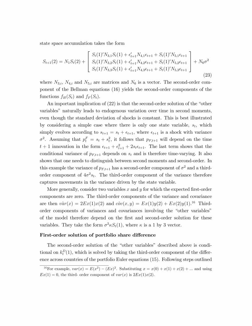
where N3;i, N4;i and N5;i are matrices and N6 is a vector. The second-order com-

ponent of the Bellman equations (16) yields the second-order components of the

functions fH(St) and fF (St).

An important implication of (22) is that the second-order solution of the �other

variables�naturally leads to endogenous variation over time in second moments,

even though the standard deviation of shocks is constant. This is best illustrated

by considering a simple case where there is only one state variable, st, which

simply evolves according to st+1 = st + �t+1, where �t+1 is a shock with variance

�2. Assuming that pFt = st + s2t , it follows that pF;t+1 will depend on the time

t + 1 innovation in the form �t+1 + �2t+1 + 2st�t+1. The last term shows that the

conditional variance of pF;t+1 depends on st and is therefore time-varying. It also

shows that one needs to distinguish between second moments and second-order. In

this example the variance of pF;t+1 has a second-order component of �2 and a third-

order component of 4�2st. The third-order component of the variance therefore

captures movements in the variance driven by the state variable.

More generally, consider two variables x and y for which the expected �rst-order

components are zero. The third-order components of the variance and covariance

are then ^var(x) = 2Ex(1)x(2) and ^cov(x; y) = Ex(1)y(2) + Ex(2)y(1).16 Third-

order components of variances and covariances involving the �other variables�

of the model therefore depend on the �rst and second-order solution for these

variables. They take the form �2�St(1), where � is a 1 by 3 vector.

First-order solution of portfolio share di¤erence

The second-order solution of the �other variables� described above is condi-

tional on kDt (1), which is solved by taking the third-order component of the di¤er-

ence across countries of the portfolio Euler equations (15). Following steps outlined

16For example, var(x) = E(x2) � (Ex)2. Substituting x = x(0) + x(1) + x(2) + ::: and using

Ex(1) = 0, the third- order component of var(x) is 2Ex(1)x(2).

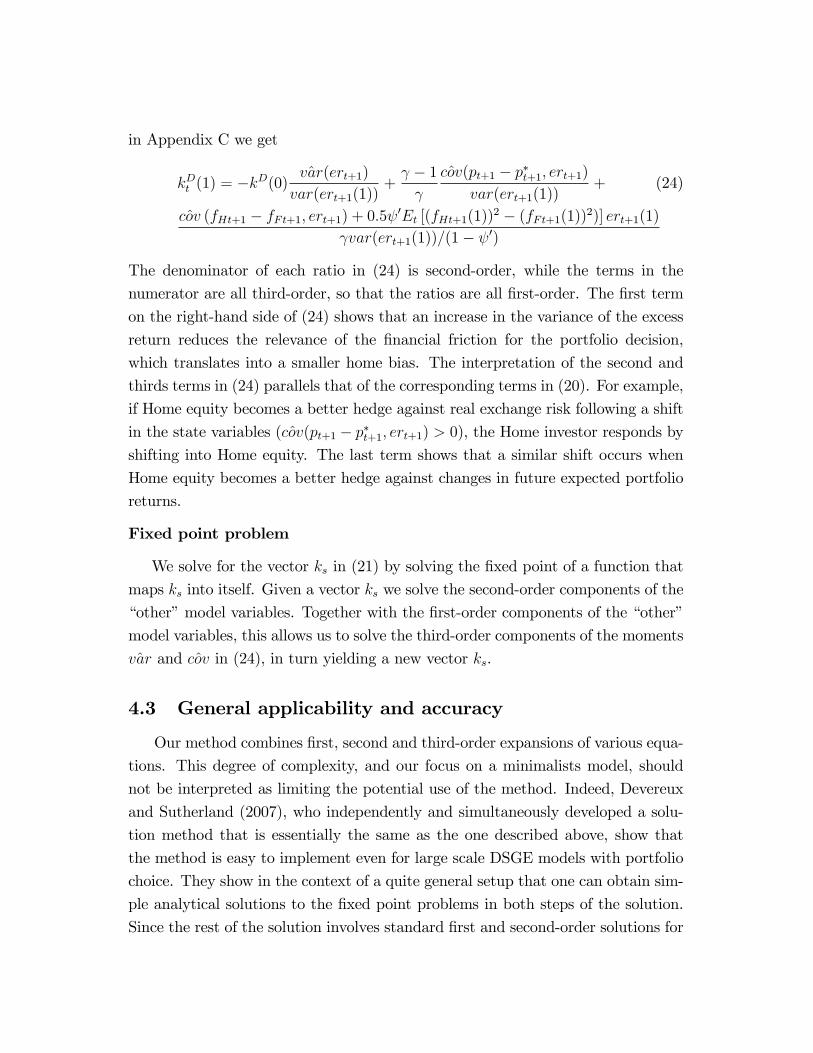
in Appendix C we get

kDt (1) = �kD(0)^var(ert+1)

var(ert+1(1))+ � 1

^cov(pt+1 � p�t+1; ert+1)

var(ert+1(1))+ (24)

^cov (fHt+1 � fFt+1; ert+1) + 0:5 0Et [(fHt+1(1))

2 � (fFt+1(1))2)] ert+1(1) var(ert+1(1))=(1� 0)

The denominator of each ratio in (24) is second-order, while the terms in the

numerator are all third-order, so that the ratios are all �rst-order. The �rst term

on the right-hand side of (24) shows that an increase in the variance of the excess

return reduces the relevance of the �nancial friction for the portfolio decision,

which translates into a smaller home bias. The interpretation of the second and

thirds terms in (24) parallels that of the corresponding terms in (20). For example,

if Home equity becomes a better hedge against real exchange risk following a shift

in the state variables ( ^cov(pt+1 � p�t+1; ert+1) > 0), the Home investor responds byshifting into Home equity. The last term shows that a similar shift occurs when

Home equity becomes a better hedge against changes in future expected portfolio

returns.

Fixed point problem

We solve for the vector ks in (21) by solving the �xed point of a function that

maps ks into itself. Given a vector ks we solve the second-order components of the

�other�model variables. Together with the �rst-order components of the �other�

model variables, this allows us to solve the third-order components of the moments

^var and ^cov in (24), in turn yielding a new vector ks.

4.3 General applicability and accuracy

Our method combines �rst, second and third-order expansions of various equa-

tions. This degree of complexity, and our focus on a minimalists model, should

not be interpreted as limiting the potential use of the method. Indeed, Devereux

and Sutherland (2007), who independently and simultaneously developed a solu-

tion method that is essentially the same as the one described above, show that

the method is easy to implement even for large scale DSGE models with portfolio

choice. They show in the context of a quite general setup that one can obtain sim-

ple analytical solutions to the �xed point problems in both steps of the solution.

Since the rest of the solution involves standard �rst and second-order solutions for

the �other variables�, the solution is no more involved than for models without

portfolio choice, and the model can be solved using standard software packages for

the �rst and second-order solutions.

Another potential issue relates to the accuracy of the solution method. It is

important to note that the issue of accuracy is no di¤erent than for DSGE models

without portfolio choice that are solved with �rst or second-order solution methods.

It is certainly possible to write down models where local approximations can be

far o¤. An example is a model with large idiosyncratic income shocks, such as

associated with unemployment, which can lead to large deviations from the point

of approximation. However, this is a general limitation of local solution methods

and has little to do with the introduction of portfolio choice per se. The accuracy

issue is not more pronounced for our method than for standard local approximation

methods applied to models without portfolio choice.

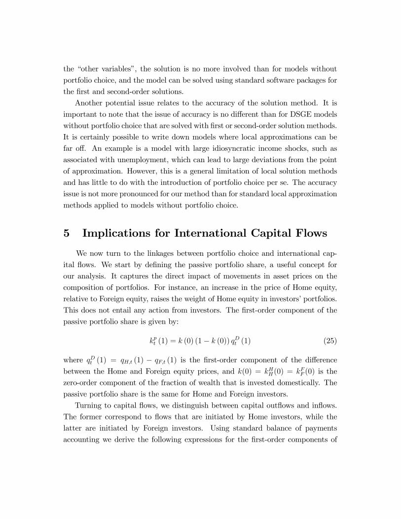
5 Implications for International Capital Flows

We now turn to the linkages between portfolio choice and international cap-

ital �ows. We start by de�ning the passive portfolio share, a useful concept for

our analysis. It captures the direct impact of movements in asset prices on the

composition of portfolios. For instance, an increase in the price of Home equity,

relative to Foreign equity, raises the weight of Home equity in investors�portfolios.

This does not entail any action from investors. The �rst-order component of the

passive portfolio share is given by:

kpt (1) = k (0) (1� k (0)) qDt (1) (25)

where qDt (1) = qH;t (1) � qF;t (1) is the �rst-order component of the di¤erence

between the Home and Foreign equity prices, and k(0) = kHH (0) = kFF (0) is the

zero-order component of the fraction of wealth that is invested domestically. The

passive portfolio share is the same for Home and Foreign investors.

Turning to capital �ows, we distinguish between capital out�ows and in�ows.

The former correspond to �ows that are initiated by Home investors, while the

latter are initiated by Foreign investors. Using standard balance of payments

accounting we derive the following expressions for the �rst-order components of

capital out�ows and in�ows:

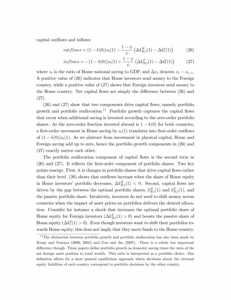
outflows = (1� k(0))st(1)�1�

��kHH;t(1)��k

pt (1)

�(26)

inflows = �(1� k(0))st(1) +1�

��kFH;t(1)��k

pt (1)

�(27)

where st is the ratio of Home national saving to GDP, and �xt denotes xt � xt�1.A positive value of (26) indicates that Home investors send money to the Foreign

country, while a positive value of (27) shows that Foreign investors send money to

the Home country. Net capital �ows are simply the di¤erence between (26) and

(27).

(26) and (27) show that two components drive capital �ows, namely portfolio

growth and portfolio reallocation.17 Portfolio growth captures the capital �ows

that occur when additional saving is invested according to the zero-order portfolio

shares. As the zero-order fraction invested abroad is 1 � k(0) for both countries,

a �rst-order movement in Home saving by st(1) translates into �rst-order out�ows

of (1� k(0))st(1). As we abstract from investment in physical capital, Home and

Foreign saving add up to zero, hence the portfolio growth components in (26) and

(27) exactly mirror each other.

The portfolio reallocation component of capital �ows is the second term in

(26) and (27). It re�ects the �rst-order component of portfolio shares. Two key

points emerge. First, it is changes in portfolio shares that drive capital �ows rather

than their level. (26) shows that out�ows increase when the share of Home equity

in Home investors�portfolio decreases, �kHH;t(1) < 0. Second, capital �ows are

driven by the gap between the optimal portfolio shares, kHH;t(1) and kFH;t(1), and

the passive portfolio share. Intuitively, investors do not need to shift money across

countries when the impact of asset prices on portfolios delivers the desired alloca-

tion. Consider for instance a shock that increases the optimal portfolio share of

Home equity for Foreign investors (�kFH;t(1) > 0) and boosts the passive share of

Home equity (�kpt (1) > 0). Even though investors want to shift their portfolios to-

wards Home equity, this does not imply that they move funds to the Home country.17The distinction between portfolio growth and portfolio reallocation has also been made by

Kraay and Ventura (2000, 2003) and Guo and Jin (2007). There is a subtle but important

di¤erence though. These papers de�ne portfolio growth as domestic saving times the ratio of the

net foreign asset position to total wealth. This ratio is interpreted as a portfolio choice. Our

de�nition allows for a more general equilibrium approach where decisions about the external

equity liabilities of each country correspond to portfolio decisions by the other country.

If movements in equity prices raise the passive portfolio share beyond its desired

level (�kpt (1) > �kFH;t(1)), investors will undo the excess passive portfolio shift by

selling Home equity and reallocating funds to Foreign equity. This corresponds to

a negative in�ow in (27). These points are summarized in our �rst result:

Result 1 Capital in�ows and out�ows can be broken into a portfolio growth and aportfolio reallocation component. The portfolio growth component captures capital

�ows that result when saving is invested in line with the zero-order portfolio shares.

The portfolio reallocation component captures capital �ows driven by �rst-order

changes in portfolio shares, relative to the passive portfolio share.

In order to understand the determinants of the portfolio reallocation component

in (26)-(27), we need to derive expressions for the optimal portfolio shares. The

�rst-order components of the portfolio shares for each country can be computed

from the average and di¤erence of portfolio shares across countries, kAt (1) and

kDt (1).18 (24) shows that the �rst-order component of the di¤erence in portfolio

shares, kDt (1), is entirely driven by the third-order component of second moments.

These ^var and ^cov terms re�ect time-variation in second moments associated with

changes in the state space. It is important to note that these terms arise endoge-

nously even though the variance of shocks is kept constant.

Result 2 Even when the standard deviation of model innovations is constant,the second moments a¤ecting portfolio choice endogenously vary over time with

changes in the state space.

The expression (24) for kDt (1) was computed using the third-order component

of the di¤erence in portfolio Euler equation across countries. We can similarly

compute kAt (1) from the third-order component of the average of portfolio Euler

equations across countries. Following steps outlined in Appendix C we write:19

kAt (1) =Etert+1(3)

var(ert+1(1))+

^covAtvart (ert+1 (1))

(28)

18Speci�cally: kHH;t(1) = kAt (1) + 0:5kDt (1) and k

FH;t(1) = kAt (1)� 0:5kDt (1).

19kAt (1) is solved in the �rst step of the solution. That solution was a result of a supply perspec-

tive, using the fact that the average portfolio share is related to relative asset supplies through

asset market clearing. Equation (28) follows from a demand (or portfolio choice) perspective. In

equilibrium the expected excess return adjusts to reconcile these two perspectives.

where:

^covAt = � 12

�^cov(pt+1 + p�t+1; ert+1)� ^var(rH;t+1) + ^var(rF;t+1)

�+1� 0

2 ^cov (fHt+1 + fFt+1; ert+1)

+ 0 (1� 0)

4 Et�(fHt+1(1))

2 + (fFt+1(1))2)�ert+1(1)

(28) shows that the �rst-order component of kAt (1) depends on time-varying second

moments, denoted by ^covAt . In addition, kAt (1) is a¤ected by the time-varying

expected excess return on Home equity, Etert+1(3). The latter does not enter

kDt (1) as Home and Foreign investors respond to expected returns in the same

way.

Result 3 Changes over time in optimal portfolio shares are associated with timevariation in expected excess returns and second moments. Second moments that

a¤ect portfolio choice involve asset returns, goods prices and future expected port-

folio returns. The third-order component of expected excess returns and second

moments a¤ects the �rst-order component of portfolio shares.

It would be tempting to conclude from the results so far that capital �ows are

driven by portfolio growth, as well as time-varying expected returns and second

moments that enter (24) and (28). This inference is not accurate however, as

capital �ows (26)-(27) are driven by the gap between the optimal and passive

portfolio shares.

It is useful to derive the equilibrium expected excess return on Home equity

to shed further light onto the determinants of capital �ows. Using the �rst-order

component of the asset market equilibrium (11)-(12), we write:

�kAt (1)��kpt (1) = �

1

2

1� kD(0)st(1) (29)

Intuitively, an increase in Home saving (and therefore drop in Foreign saving) raises

the demand for Home equity in the presence of portfolio home bias (kD(0) > 0).

Asset market clearing requires either an increase in the relative supply of Home

equity through a higher asset price, which raises the passive portfolio share�kpt (1),

or a decrease in the demand for Home equity through a shift in the world portfolio

away from Home equity (�kAt (1) < 0).

Combining (28) and (29) gives an expression for changes in expected excess

return:

�Etert+1(3) = �Etert+1(3)S +�Etert+1(3)

P +�Etert+1(3)TVM (30)

where:

�Etert+1(3)S = � vart(ert+1(1))

1

2

1� kD(0)st(1)

�Etert+1(3)P = vart(ert+1(1))�k

pt (1)

�Etert+1(3)TVM = �� ^covAt

(30) shows that there are three determinants of expected excess return changes.

The �rst, �Etert+1(3)S, re�ects saving. Intuitively, higher saving in the Home

country boost the relative demand for Home equity due to home bias (kD(0) >

0). The expected excess return on Home equity needs to fall to switch asset

demand toward Foreign equity and clear asset markets. The second determinant,

�Etert+1(3)P , is associated with changes in the passive portfolio share. An increase

in the relative price of Home equity raises the relative supply of Home equity. Asset

market clearing requires a shift of asset demand towards Home equity, which is

achieved through an increase in the expected excess return on Home equity. The

last determinant, �Etert+1(3)TVM , re�ects time-varying second moments. When

these moments boost the world demand for Home equity (�covAt > 0), asset market

clearing requires an o¤setting reduction in asset demand through a lower expected

excess return on Home equity.

In addition, we can show from the �rst and second-order component of the

average of portfolio Euler equations (15) that both the �rst and second-order com-

ponents of the expected excess return are zero (Etert+1(1) = Etert+1(2) = 0). (30)

therefore captures the total change in the expected excess return up to third-order

accuracy. Our results for the expected excess return are summarized as:

Result 4 Changes in expected excess returns are associated with (i) saving, (ii)changes in relative asset prices, and (iii) time-varying second moments that a¤ect

the average portfolio share. Changes in expected excess returns are small (third-

order).

We now turn to the link between the expected excess returns and capital �ows.

Since Home and Foreign investors have the same expectations, expected excess

returns a¤ect capital �ows only through the average portfolio share, not the dif-

ference in portfolio shares. Combining (28) and (30) the di¤erence between the

change in the average portfolio share and the passive portfolio share is

�kAt (1)��kpt (1) =

�Etert+1(3)S

var(ert+1(1))(31)

Intuitively, an increase in Home saving boosts the relative demand for Home eq-

uity because of portfolio home bias. Asset market clearing requires an o¤setting

reduction in the demand through a lower expected excess return on Home equity.

Investors across the world reallocate their portfolio towards Foreign equity, leading

to a capital �ow out of the Home country (�kAt (1)��kpt (1) < 0).

(31) shows that the average portfolio reallocation is not driven by the over-

all change in the expected excess return, but only by the component associated

with saving. By contrast, the components associated with asset price changes,

�Etert+1(3)P , and time-varying second moments, �Etert+1(3)TVM , entail no cap-

ital �ows.

Result 5 There is no straightforward link between changes in the expected excessreturn and capital �ows. Changes in the equilibrium expected excess return associ-

ated with changes in relative asset prices, or with time-varying second moments, do

not generate capital �ows. Only the changes associated with saving lead to portfolio

reallocation that a¤ects capital �ows.

We are now ready to present the drivers of capital �ows. Using (31), capital

�ows (26)-(27) are written as:

outflows = (1� k(0))st(1)�1�

�Etert+1(3)S

var(ert+1(1))� 1�

�kDt (1)

2(32)

inflows = �(1� k(0))st(1) +1�

�Etert+1(3)S

var(ert+1(1))� 1�

�kDt (1)

2(33)

As described above, the portfolio growth component re�ects the investment of

saving based on the zero-order portfolio allocation. Movements in expected excess

returns that are linked to saving a¤ect capital in�ows and out�ows with opposite

signs. Finally, time-varying second moments that a¤ect the di¤erence in portfolio

shares, kDt (1), a¤ect capital in�ows and out�ows with the same sign.

Result 6 Capital out�ows and in�ows are driven by three factors. The �rst is aportfolio growth component. The second is associated with time-varying expected

excess return on Home equity, but only a component of it. The third is associated

with time-varying second moments, but only to the extent that they a¤ect Home

and Foreign portfolio allocation di¤erently.

(32) and (33) also have implications for net capital �ows and for the co-

movement between capital in�ows and out�ows. The di¤erence between (32) and

(33) shows that net �ows only re�ect the �rst two components and are therefore

not a¤ected by kDt (1). By contrast, the sum of gross capital �ows only re�ects the

di¤erence in portfolio shares kDt (1). Changes in second moments that drive kDt (1)

lead to a positive co-movement between capital in�ows and capital out�ows. For

instance, and increase in the portfolio share di¤erence (�kDt (1) > 0) leads to both

negative out�ows and in�ows as all investors repatriate money towards their own

country.20

Result 7 Capital in�ows and out�ows are positively correlated when there is su¢ -cient time-variation in second moments that a¤ect Home and Foreign portfolios dif-

ferently. This is the only element in the model that leads to a positive co-movement

between capital in�ows and out�ows.

6 A numerical illustration

6.1 Parameterization

We illustrate the implications of our simple model through a numerical exam-

ple. The parameterization we adopt is for illustrative purposes only, not to match

the data of any particular country. Nonetheless, we discuss the empirical relevance

of the model at a qualitative level at the end of this section.

We assume a labor share of output, �, of 0:7. Productivity shocks are assumed

to be highly persistent, with � = 0:99. Productivity innovations have a standard

deviation of � = 5%. Turning to consumers�preferences, we assume home bias

20The negative co-movement between in�ows and out�ows due to portfolio growth is an artifact

of the absence of investment in the model. More generally Home and Foreign saving could move

together when there are corresponding changes in global investment since world saving equals

world investment.

in preferences by setting � = 0:8. The elasticity of substitution between Home

and Foreign goods is set at � = 2. The rate of relative risk-aversion, , is set

at 10 and � = 1. Agents face a probability of death of = 0:05, leading to a

consumption-wealth ratio of 5%. The transaction cost on investing abroad, � , is

set at 0:419%. These parameters generate a sizable home bias in equity holdings,

with the zero-order component of the fraction invested in domestic equity equal

to 0.8.21 We consider the dynamic response of the economy to a 5% increase in

Home productivity.

6.2 Real exchange rate and equity prices

Chart 1 illustrates the dynamic response of the relative price of the Foreign

good. The increase in Home productivity boosts the supply of the Home good,

leading to an immediate increase in the relative price of the Foreign good (a Home

real depreciation). This is followed by a gradual reduction (Home real apprecia-

tion) as the shock dissipates. Chart 2 shows the dynamic response of equity prices,

depicting the Home equity price in units of the Home good and the Foreign eq-

uity price in units of the Foreign good. The persistent Home productivity shock

immediately raises the Home equity price. It also leads to a small increase in the

Foreign equity price as some of the additional wealth stemming from the higher

productivity is invested in Foreign equity. While the increase in Foreign equity

prices is larger when expressed in Home goods, Home equity prices still increase

by more on impact. Equity prices subsequently move back to the steady state,

which implies a larger expected drop in the Home equity price than in the Foreign

equity price.

6.3 Capital �ows

Chart 3 shows the response of gross and net capital �ows from the perspective

of the Home country, expressed as a fraction of initial GDP. The positive income

shock in the Home country boosts income more than wealth and consumption,

21This implies that agents invest 30% more in the domestic country than under perfect diver-

si�cation. Of this, there is a bias of +67% invested in the domestic country due to the �nancial

friction � , a negative bias of -40% due to a negative correlation between the real exchange rate

and excess return (this is a foreign bias) and a positive home bias of +3% due to the hedge

against changes in expected portfolio returns.

leading to a rise in saving and a net capital out�ow. Initially both capital in�ows

and out�ows go down, with investors from both countries selling assets abroad

and bringing the money to their own country. By contrast, in subsequent periods

investors from both countries shift funds to the Foreign country, so that the Home

country experiences positive capital out�ows and negative capital in�ows.

Portfolio reallocation

We know from (26) and (27) that capital �ows are driven by portfolio growth

and portfolio reallocation. The latter is associated with changes in portfolio shares

in deviation from the passive portfolio share. Chart 4 shows the impact of the

shock on both the passive portfolio share invested in Home equity and the opti-

mal portfolio shares of Home and Foreign investors invested in Home equity. The

increase in Home equity prices automatically boosts the value of investors�hold-

ings of Home equity and raises the passive portfolio share. The optimal portfolio

share di¤ers across investors, with Home investors choosing a larger share of Home

equity in their portfolio than Foreign investors (kDt (1) > 0). The Home portfo-

lio share exceeds the passive portfolio share, leading Home investors to actively

reallocate their portfolio by selling Foreign equity to buy Home equity. By con-

trast, the Foreign portfolio share is lower than the passive portfolio share, so that

Foreign investors actively reallocate their portfolio towards Foreign assets. This

retrenchment towards domestic assets accounts for the negative capital in�ows and

out�ows in Chart 3 in the immediate response to the shock. After the initial shock

the gradual reduction in the price of Home equity leads to a gradual decrease in the

passive portfolio share. As the reduction in the optimal portfolio shares of both

Home and Foreign investors is more pronounced, they both actively reallocate their

portfolio towards Foreign assets, accounting for the positive capital out�ows and

negative capital in�ows in Chart 3.

Components of capital �ows

Charts 5 and 6 show the three components of capital �ows that are represented

in (32) and (33). The portfolio growth component leads to positive capital out�ows

and negative capital in�ows (thin line). The productivity increase in the Home

country boosts Home saving. This leads to increased capital out�ows as 20% of the

increase in Home saving is invested in the Foreign country. The drop in Foreign

saving leads to a drop in capital in�ows.

The other two components re�ect portfolio reallocation. The dotted lines rep-

resents changes in the expected excess return. As a result of portfolio Home bias,

the rise in Home saving leads to an excess demand for Home equity. A drop in

the expected excess return on Home equity is then needed to clear asset markets.

This leads to a reallocation of portfolios towards Foreign equity, so that capital

out�ows are positive and capital in�ows are negative.

The last component is associated with time-varying second moments and is

represented by the thick lines. We have seen that changes in second moments only

a¤ect capital �ows to the extent that they a¤ect portfolios of Home and Foreign

investors di¤erently. This is re�ected in the immediate increase in kDt at the time

of the shock. An increase in the volatility of the excess return at the time of the

shock leads to a reduction in home bias. This is however more than o¤set by an

increase in the covariances between the excess return on the one hand and the

real exchange rate and the hedging component on the other hand. This leads to

increased home bias: kDt (1) > 0. From (32) and (33) this translates into negative

capital in�ows and out�ows.

While time-varying second moments have a very large transitory impact on

capital �ows, portfolio growth and changes in expected excess returns have a much

more persistent impact. The di¤erence can be understood as follows. Persistence

in the state variables, due to the highly persistent technology shocks, leads to long-

lasting changes in the level of saving and second moments. The portfolio growth

and expected excess return components of capital �ows both depend on the level

of saving and therefore inherit its persistence. By contrast, the third component

is driven by changes in second moments, which have very little persistence. Time-

varying second moments therefore have a large impact at the time of shock, when

they change substantially, but not thereafter as they change only very gradually.

This can be seen in Chart 4 where the home bias kDt (1) remains stable after the

initial increase.

Disconnect between capital �ows and expected return changes

(30) and (31) show a disconnect between capital �ows and changes in the

expected excess return, as only one component of the latter a¤ects capital �ows.

This is illustrated by Chart 7 which shows the equilibrium expected excess return

as well as its three components. The overall expected excess return on Home

equity rises in response to the shock, while the only component that a¤ects capital

�ows� associated with the level of saving� drops. It is the drop in the expected

excess return due to higher Home saving that leads to increased capital out�ows

and lower capital in�ows, as documented by the broken lines in Charts 5 and 6.

The other two components of the equilibrium expected excess return are both

positive and much larger. The higher relative price of Home equity boosts the

relative supply of Home equity. In order to clear �nancial markets, the demand for

Home equity needs to be raised through higher expected returns. As the passive

portfolio involves no asset trade, there are no capital �ows associated with this.

Finally, the average portfolio share kAt invested in Home equity drops due to time-

varying second moments, ^covAt . To clear asset markets this is o¤set by higher

expected returns on Home equity, with no implication for capital �ows.

Capital �ows under a simulation of the model

Our analysis so far focuses on the impulse responses to a particular shock.

We can draw implications for the co-movements and volatility of capital �ows

by simulating the model over 30 periods. The three components of capital �ows

in (32) and (33) are presented in Chart 8 and 9 for capital out�ows and in�ows,

respectively. Both charts clearly show that time-varying second moments drive the

volatility of capital �ows, while expected excess returns and portfolio growth drive

their persistence. In addition, the time-varying second moments lead to a positive

correlation between out�ows and in�ows, while the other two components imply

a negative correlation. Total capital out�ows and in�ows are presented in Chart

10. Under our parameterization, the dominant in�uence of time-varying second

moments leads to a positive correlation (0.34) between capital in�ows and out�ows.

A lower persistence of technology shocks would lead to an even higher correlation

between capital in�ows and out�ows as the portfolio growth and expected excess

return components of capital �ows would be less persistent.

6.4 Valuation e¤ects and return di¤erentials

Recent contributions point to substantial valuation e¤ects that capture the im-

pact of changing asset prices and exchange rates on the value of external assets and

liabilities. In addition, expected valuation e¤ects can play a role on the �nancing

of external imbalances. We now turn to the role of these channels in our model.

Impact on the value of external assets and liabilities

As illustrated in Charts 11 and 12, unexpected valuation e¤ects have large

e¤ects on the value of outstanding external assets and liabilities. Chart 11 shows

the paths of gross external assets and liabilities of the Home country, as well as

its net external asset position, while Chart 12 presents the net external position

together with cumulative net capital �ows. The initial response of both gross assets

and liabilities is almost entirely due to unexpected valuation e¤ects. Speci�cally,

the increase in the price of Home equity boosts the value of liabilities to Foreign

investors. In addition, the real depreciation of the Home currency raises the value

of Home investors�holdings in the Foreign country. The �rst e¤ect is larger and the

Home country becomes a net debtor. After the initial shock gross liabilities drop

much faster than gross assets and soon the Home country becomes a net creditor.

Chart 12 shows that this is driven to a large extent by cumulative net capital

out�ows. In addition the Home country bene�ts from fully expected valuation

gains, primarily re�ecting the gradual fall in the price of the Home equity that

reduces the value of external liabilities. The positive expected valuation e¤ects are

illustrated by the decreasing gap between cumulative capital out�ows and the net

external position in Chart 12.

External adjustment

Gourinchas and Rey (2007) show that expected valuation e¤ects may play an

important role in �nancing a positive external debt. An expected depreciation of

the dollar boost the dollar return on the U.S. investors�foreign holdings, a channel

that could contribute to �nancing the U.S. external debt. Using standard balance

of payments accounting within the context of our model we write:

�nfat(1) =1Xs=1

Ettbt+s(1)

R(0)s+GA(0)

1Xs=1

Et(rF;t+s(1)� rH;t+s(1))

R(0)s�1(34)

where nfa is the net foreign asset position, tb is the trade balance and GA(0) is the

zero-order component of gross assets. (34) shows that a net external debt can be

�nanced by either expected future trade surpluses or by more favorable expected

future returns on external assets (Foreign equity) than external liabilities (Home

equity).

The expected return di¤erential in (34) re�ects three factors: valuation changes

associated with the real exchange rate, valuation changes associated with equity

prices, and dividend payments. A net external debt can then be repaid through

four channels: (i) the present value of expected future trade surpluses, (ii) the

present value of expected valuation gains associated with the real exchange rate,

(iii) the present value of expected valuation gains associated with equity prices and

(iv) the present value of expected di¤erences between Home and Foreign dividend

yields.

Under our parametrization, a 5% increase in Home productivity leads to a net

external debt of 6.2% of GDP on impact. Chart 13 shows how this debt is �nanced

by the four factors listed above. Expected valuation e¤ects are large: the expected

real appreciation of the Home currency generates valuation losses that amount to

5.1% of GDP in present value terms. On the other hand, the expected fall in Home

equity prices, relative to Foreign equity prices, translates into an expected gain for

the Home country equal to 7.2% of GDP in present value terms. Overall valuation

e¤ects therefore amount to a net gain of 2.1%, which represents a third of the net

external debt.

While valuation e¤ects are important, they do not translate into a predictable

return di¤erential as they are exactly o¤set by di¤erences in expected dividend

yields. As Home productivity is persistently higher, the expected dividend yield

is larger for Home than Foreign equity. The resulting net dividend payment to

Foreign investors amount to 2.1% of GDP in present value terms. The three

factors that enter expected returns then cancel out and the next external debt is

entirely repaid through future trade surpluses.

This result is driven by the fact that the expected �rst-order component of the

excess return is zero, a general implication of arbitrage in portfolio choice. Taking

the �rst-order component of (15) shows that the expected �rst-order component

of expected returns must be the same for all assets. This condition can only be

relaxed by introducing elements that break the arbitrage across various assets.22

22One example is Bacchetta and van Wincoop (2007), who introduce a portfolio decision mak-

ing cost (or asset management cost), leading to infrequent portfolio decisions.

6.5 Relation to the Data

Our numerical illustration is meant to merely outline the main implications of

the model. While we do not undertake a formal empirical test of the model, many

of its qualitative features are consistent with a broad set of empirical evidence.

In terms of capital �ows data, both Kraay and Ventura (2003) and Guo and

Jin (2007) �nd that in the short-run portfolio reallocation is a far more important

source of capital �ow �uctuations than portfolio growth, in line with our model.

Also relevant is the evidence reported in Hau and Rey (2007). They use data on

stock holdings of thousands of global mutual funds and �nd that funds actively

reallocate towards Foreign stock following an increase in the relative return on

Home stock relative to Foreign stock. This is consistent with the active realloca-

tion towards Foreign stock in our model by both Home and Foreign investors after

the initial period of the shock.23 Hau and Rey (2007) refer to this aspect as port-

folio rebalancing, an aspect that is exactly the same as our de�nition of portfolio

reallocation. In addition the model can account for a positive correlation between

capital in�ows and out�ows. For the United States the unconditional correlation

between capital in�ows and out�ows (share of GDP) is 0.83 for annual data from

1970 through 2006 and 0.64 for quarterly data.24

The model illustrates the links between time-varying second moments and cap-

ital �ows and between time-varying expected returns and capital �ows. To our

knowledge, no empirical work has yet been done on the link between time-varying

second moments and capital �ows. This will be an important area of future research

given the central role of time-varying risk in the model. The �nance literature has

extensively documented the time-varying nature of both variances and covariances

of asset returns, with changes in second moments being quite persistent. This

aspect is captured by a variety of statistical models, including ARCH or GARCH

models and stochastic-volatility models.25 In our model, the time-varying nature

of second moments is entirely endogenous and follows naturally from the solution

method. Also consistent with the data, changes in second-moments are highly

23Even though portfolio reallocation di¤ers signi�cantly between Home and Foreign investors

during the period of the shock, the model implies that even then Home and Foreign investors on

average reallocate towards Foreign stock.24For changes in in�ows and out�ows these correlations are respectively 0.80 and 0.84.25For a brief overview of this large literature, see Campbell, Lo and MacKinlay (1997), chapter

12.

persistent as they inherit the persistence of the state variables.

In a recent paper, Didier and Lowenkron (2007) set out to illustrate the link

between time-varying expected returns and net capital �ows. Using data for the

United States and Japan, they estimate a VAR involving US and Japanese asset

returns and other �nancial variables. The resulting time-varying expected excess

returns are applied to a simple portfolio choice model to develop the implications

for net capital �ows. While the implied theoretical net capital �ows are positively

correlated with actual net capital �ows, they are much more volatile (by a factor

300) than net capital �ows in the data. This suggests that either actual expected

excess returns are far smaller or that components of expected excess returns do

not a¤ect capital �ows. This is consistent with the theory, which tells us that

equilibrium expected excess returns that drive net capital �ows are third-order

and that a large component of expected excess returns do not impact capital �ows.

The recent evidence by Curcuru, Dvorak and Warnock (2008) is also consistent

with small expected excess returns. While they do not consider the time-varying

nature of expected excess returns, they �nd that the average di¤erence between

the return on U.S. assets and liabilities is negligible within asset classes (bonds or

stocks).26

The model implies that unexpected valuation e¤ects have a large impact on

the value of external assets and liabilities. In the short-run these can signi�cantly

outweigh the impact of net capital �ows on the net foreign asset position. This

is consistent with recent evidence on the importance of valuation e¤ects, such as

Gourinchas and Rey (2007), Lane and Milesi-Ferretti (2005) and Tille (2008). Val-

uation e¤ects have received signi�cant attention in recent years as they interact

with rapidly increasing levels of external assets and liabilities.27 The model also

implies that expected valuation e¤ects can be very large. However, the model im-

plies that predictable di¤erences in expected returns cannot contribute to �nancing

a net external debt to the �rst-order, in contrast to the empirical �ndings by Gour-

inchas and Rey (2007). We cannot rule out that the third-order component of the

expected excess return plays this role, but these third-order components are very

small.26Based on data from 1986 to 2005 they �nd that the average returns on US assets and liabilities

are respectively 13.1% and 13.8% for stock and 9.3% and 8.7% for bonds.27For industrialized countries the sum of external assets and liabilities as a fraction of GDP

has increased from less than 50% in the 1970s to about 350% today.

7 Conclusion

We develop a simple two-country DSGE model with portfolio choice in order

to shed light on the implications of portfolio choice for international capital �ows.

We show that capital �ows are driven by three factors: portfolio growth, portfolio

reallocation associated with time-varying expected returns, and portfolio reallo-

cation associated with time-varying second moments, with the last two playing a

sizable role. We also �nd that several important factors that determine equilibrium

expected return di¤erences have no e¤ect on capital �ows. We stress the relevance

of endogenous variations in second moments, even though the standard deviation

of model innovations is constant. These changing second moments a¤ect capital

�ows only to the extent that they a¤ect domestic and foreign investors di¤erently,

and lead to positive co-movements between capital in�ows and out�ows.

An additional contribution of the paper is to develop a widely applicable

method for solving DSGE models with portfolio choice. The solution method

stays very close to standard �rst and second-order solution methods. While our

focus here has been on international capital �ows, the method can be used to ad-

dress many other types of questions where portfolio choice may be relevant. Open

economy DSGE models no longer need to be restricted to a single traded bond or

complete markets.

While the model is qualitatively consistent with a broad range of empirical evi-

dence, an important agenda for future research is to more formally connect general

equilibrium portfolio choice models to the empirical evidence on capital �ows and

international asset holdings. The main goal of this research should be to match

some key aspects of the data, such as the level of external (and bilateral) asset

holdings, the volatility of gross and net capital �ows, the co-movement between

capital in�ows and out�ows and the relationship between capital �ows and asset

prices. The large empirical �nance literature on time-varying second moments

can potentially shed light on the link between capital �ows and changing sec-

ond moments. Another relevant line of research focuses on the empirical evidence

for the di¤erent components of capital �ows, such as di¤erent asset categories and

portfolio growth versus portfolio reallocation. In parallel to the international trade

literature, gravity models for bilateral asset positions can be developed that inform

us of the magnitude and determinants of international �nancial frictions.

The model discussed in this paper was kept simple in order to focus on the

role of portfolio choice while abstracting from other choice variables that are not

key to the analysis here. Future work will need to introduce consumption and

investment decisions as well. Other natural extensions are to introduce monetary

elements, �scal policy, additional assets and multiple countries. A potentially

rewarding strategy may also be to introduce information asymmetries as in the

noisy rational expectations literature in �nance. All these extensions will put us

in a better position to confront the model to data on gross and net capital �ows

and external asset holdings, analyze policy questions related to capital �ows, and

make meaningful predictions related to the external adjustment process faced by

countries with large external imbalances.

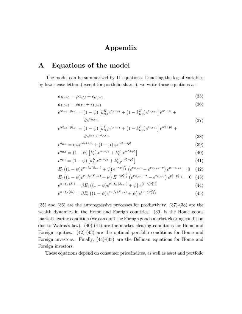
Appendix

A Equations of the model

The model can be summarized by 11 equations. Denoting the log of variables

by lower case letters (except for portfolio shares), we write these equations as:

aH;t+1 = �aH;t + �H;t+1 (35)

aF;t+1 = �aF;t + �F;t+1 (36)

ewt+1+pt+1 = (1� )�kHH;te

rH;t+1 + (1� kHH;t)erF;t+1

�ewt+pt +

�eaH;t+1 (37)

ew�t+1+p

�t+1 = (1� )

�kFH;te

rH;t+1 + (1� kFH;t)erF;t+1

�ew

�t+p

�t +

�epFt+1+aF;t+1 (38)

eaH;t = � ewt+�pt + (1� �) ew�t+�p

�t (39)

eqH;t = (1� )�kHH;te

wt+pt + kFH;tew�t+p

�t�

(40)

eqF;t = (1� )�kHF;te

wt+pt + kFF;tew�t+p

�t�

(41)

Et�(1� )ev+fH(St+1) +

�e� r

p;Ht+1�erH;t+1 � erF;t+1��

�ept�pt+1 = 0 (42)

Et�(1� )ev+fF (St+1) +

�E� r

p;Ft+1�erH;t+1�� � erF;t+1

�ep

�t�p�t+1 = 0 (43)

ev+fH(St) = �Et�(1� )ev+fH(St+1) +

�e(1� )r

p;Ht+1 (44)

ev+fF (St) = �Et�(1� )ev+fF (St+1) +

�e(1� )r

p;Ft+1 (45)

(35) and (36) are the autoregressive processes for productivity. (37)-(38) are the

wealth dynamics in the Home and Foreign countries. (39) is the Home goods

market clearing condition (we can omit the Foreign goods market clearing condition

due to Walras�s law). (40)-(41) are the market clearing conditions for Home and

Foreign equities. (42)-(43) are the optimal portfolio conditions for Home and

Foreign investors. Finally, (44)-(45) are the Bellman equations for Home and

Foreign investors.

These equations depend on consumer price indices, as well as asset and portfolio

returns, which in logarithmic form can be written as

e(1��)pt = �+ (1� �) e(1��)pFt (46)

e(1��)p�t = (1� �) + �e(1��)pFt (47)

erH;t+1 = eqH;t+1�qH;t + (1� �)eaH;t+1�qH;t (48)

erF;t+1 = eqF;t+1�qF;t + (1� �)epFt+1+aF;t+1�qF;t (49)

erp;Ht+1 =

�kHH;te

rH;t+1 + (1� kHH;t)erF;t+1��

�ept�pt+1 (50)

erp;Ft+1 =

�kFH;te

rH;t+1�� + (1� kFH;t)erF;t+1

�ep

�t�p�t+1 (51)

(46)-(47) de�ne the consumer prices indexes. (48)-(49) de�ne the rates of return

on Home and Foreign equity. Finally, (50)-(51) de�ne the rates of return on the

portfolios of Home and Foreign investors.

B Expansions of the Bellman equation

The state variables of the model are given by (18). The zero-order components

of the logs of productivity are zero. Similarly, wealth is identical in both coun-

tries to a zero-order, implying that the zero-order component of the cross-country

di¤erence in (logs) of wealth is zero. This implies S (0) = 0. The elements of

the Bellmann equation for the Home investor (44) are solved by taking a second-

order expansion around S (0). The resulting expression contains both �rst- and

second-order components. The �rst-order components are:

v (1) +H1;HSt (1) = (1� 0) [v (1) +H1;HEtSt+1 (1)] + Et(1� )rp;Ht+1 (1) (52)

where v (1) is the �rst-order component of v, H1;H is a 1x3 vector with the �rst

derivative of fH(S), evaluated at S (0), and 0 = 1 � �(1 � )R(0)1� . (52) is

solved by v (1) = 0 and:

H1;H = (1� )rs (I3 � (1� 0)N1)�1

where rs is a 1x3 matrix taken from the �rst-order solution of the portfolio return

for the Home investor. From the �rst-order solution of control variables (19), we

can write rp;Ht+1 (1) = rsSt+1 (1). I3 is a 3x3 identity matrix and N1 is the 3x3 matrix

from (19).

The second-order components of (44) are:

H1;HSt (2) +1

2

�[H1;HSt (1)]

2 + 2v (2) + St (1)0H2;HSt (1)

�= (53)

(1� 0)H1;HEtSt+1 (2) + (1� )Etrp;Ht+1 (2) +

0

2Et

h(1� )rp;Ht+1 (1)

i2+

1� 0

2Et

�hH1;HSt+1 (1) + (1� )rp;Ht+1 (1)

i2+ 2v (2) + St+1 (1)

0H2;HSt+1 (1)

�where v (2) is the second-order component of v and H2;H is a 3x3 matrix with the

second derivative of fH(S), evaluated at S = 0.

(53) entails cross-products of the �rst-order components of the state variables,

St+1 (1), and the portfolio return, rp;Ht+1 (1). These terms are taken from the �rst-

order solution (19). (53) also includes the second-order components of the state

variables, St+1 (2), which are taken from (23), as well as the second-order compo-

nent of the expected the portfolio return, Etrp;Ht+1 (2), which takes a form similar to

(22):

Etrp;Ht+1 (2) = rsSt (2) + St (1)

0 rssSt (1) + r�2 (54)

where rss is a 3x3 matrix and r is a scalar.

We use (53), along with the solution for St+1 (1), St+1 (2), rp;Ht+1 (1) andEtr

p;Ht+1 (2)

to solve for H2;H .28 The 9x1 vector Hvec2;H is the "vectorized" form of the 3x3 matrix

H2;H . Speci�cally, the �rst three elements of Hvec2;H are the �rst row of H2;H , the

next three elements are the second row of H2;H and the last three elements are the

third row of H2;H . Hvec2;H is solved from (53) as:

Hvec2;H = (I9 � (1� 0)N)�1Hvec

3

where I9 is a 9x9 identity matrix. N is a 9x9 matrix that consists of cross-products

of various elements of the N1 matrix from (19). The 9x1 vector Hvec3 is the "vec-

torized" form of a 3x3 matrix H3. The matrix H3 includes cross-products of the

matrices H1;H and rs, as well as the matrix rss in the second-order component of

the expected portfolio return (54), speci�cally:

H3 = �H 01;HH1;H + 2F1 + 2(1� )rss + (1� 0)N 0

1H01;HH1;HN1

+2(1� 0)(1� )N 01H

01;Hrs + (1� )2r0srs

F1 = (1� 0)

3Xv=1

H1;H(v)N3;v

28We also solve for v (2), but this element does not a¤ect portfolio choice.

where H1;H(v) is the v�th element of the 1x3 vector H1;H and the 3x3 matrices

N3;v are the same as in (23).

The corresponding matrices for the Foreign investor, H1;F and H2;F , are com-

puted analogously.

C First-order di¤erence in portfolio shares

The solution of the �rst-order component of the portfolio share di¤erence kDtrelies on the third-order components of the optimal portfolio conditions (42)-(43).

The expansion of the condition for the Home investor (42) leads to:

Etert+1 (3) + Etert+1 (1) rAt+1 (2) + Etert+1 (2) r

At+1 (1) (55)

+Etert+1 (1)h(1� 0)fHt+1 (2)� rp;Ht+1 (2) + pt (2)� pt+1 (2)

i+Etert+1 (2)

h(1� 0)fHt+1 (1)� rp;Ht+1 (1) + pt (1)� pt+1 (1)

i+�Et

hrAt+1 (1) + (1� 0)fHt+1 (1)� rp;Ht+1 (1) + pt (1)� pt+1 (1)

i+O3 = 0

where ert+1 (i) = rH;t+1 (i) � rF;t+1 (i), rAt+1 (i) = 0:5 [rH;t+1 (i) + rF;t+1 (i)], and

� is second-order. The �rst term in (55) is the third-order component of the

expected excess return. The next two terms are the third-order components of

the cross-product between excess returns and the average return, and consists of

products of �rst- and second-order terms. Similarly, the fourth and �fth terms are

the third-order components of the cross-product between excess returns and the

pricing kernel. The sixth term re�ects the friction in investing abroad, � . The last

term in (55) consists of cubic-products of �rst-order elements:

O3 =1

6Et�(rH;t+1 (1))

3 � (rF;t+1 (1))3�

+Et

h(1� 0)fHt+1 (1)� rp;Ht+1 (1) + pt (1)� pt+1 (1)

irAt+1 (1) ert+1 (1)

+1

2(1� 0)Et

hfHt+1 (1)� rp;Ht+1 (1) + pt (1)� pt+1 (1)

i2ert+1 (1)

+1

2 0Et

h� rp;Ht+1 (1) + pt (1)� pt+1 (1)

i2ert+1 (1)

The various components of O3 are solved using the �rst-order solution (19).

We can show that the resulting expression is:

O3 = 2rDEBHAH�2St +

0(1� 0)

2Et [fHt+1(1)]

2 ert+1(1)

where AH is a 1x3 vector and rDE and BH are scalars. rDE re�ects the sensitivity

of the �rst-order excess return to innovations:

ert+1 (1) = rDE�Dt+1

where �Dt+1 = �H;t+1 � �F;t+1. AH and BH re�ect the �rst-order solution of a

combination of the average rate of return rAt+1 (1) and the pricing kernel:

rAt+1 + (1� 0)fHt+1 (1)� rp;Ht+1 (1) + pt (1)� pt+1 (1) = AHSt +BH�Dt+1 + CH�

At+1

where CH is a scalar and �At+1 = 0:5 (�H;t+1 + �F;t+1).

We undertake similar steps using the condition for the Foreign investor (43).

Taking the di¤erence between (55) and its equivalent for the Foreign investor, we

write:

0(1� 0)

2Et�[fHt+1(1)]

2 � [fFt+1(1)]2)�ert+1(1) (56)

+Etert+1(1)

"(1� 0) [fHt+1 (2)� fFt+1 (2)]�

�rp;Ht+1 (2)� rp;Ft+1 (2)

�+(pt (2)� p�t (2))�

�pt+1 (2)� p�t+1 (2)

� #

+Etert+1(2)

"(1� 0) [fHt+1 (1)� fFt+1 (1)]�

�rp;Ht+1 (1)� rp;Ft+1 (1)

�+(pt (1)� p�t (1))�

�pt+1 (1)� p�t+1 (1)

� #= 0

The �rst-order component of the di¤erence in portfolio shares, kDt (1), enters

(56) through the second-order components of the portfolio returns. Taking the

second-order components of (50)-(51) leads to:

rp;Ht+1 (2)� rp;Ft+1 (2) = kD(0)ert+1 (2) + (pt (2)� p�t (2))

��pt+1 (2)� p�t+1 (2)

�+ kDt (1) ert+1 (1)

Similarly, taking the �rst-order component of (50)-(51) leads to:

rp;Ht+1 (1)� rp;Ft+1 (1) = kD(0)ert+1 (1) + (pt (1)� p�t (1))��pt+1 (1)� p�t+1 (1)

�Using this result, (56) becomes:

0(1� 0)

2Et�[fHt+1(1)]

2 � [fFt+1(1)]2)�ert+1(1)

+(1� 0) ^cov (fHt+1 � fFt+1; ert+1)� kD(0)var(ert+1)

+ ( � 1) ^cov(pt+1 � p�t+1; ert+1)� kDt (1) var(ert+1) = 0 (57)

where ^cov (xt+1; yt+1) = Etxt+1 (1) yt+1 (2) + Etxt+1 (2) yt+1 (1) and ^var (xt+1) =

^cov (xt+1; xt+1) and var(ert+1) = Et [ert+1 (1)]2. (24) follows simply from (57).

The elements of (57) are computed by using the �rst-order solution (19), the

second-order dynamics of the state variables, (23), and the second-order solution

for the control variables, which are of the form of (22). For instance, the excess

returns are:

ert+1 (1) = r0��t+1 ert+1 (2) = St (1)0M�t+1

where r0� is a 1x2 vector, �t+1 = [�H;t+1; �F;t+1]0 and M is a 3x2 matrix. Using these

expression, we write:

var(ert+1) = 2Etert+1 (1) ert+1 (2) = 2�2r0�M

0St (1) (58)

(58) shows that the third-order components of the variances and covariances in (57)

re�ect the second-order variance of the innovations, �2, along with the �rst-order

state variables, St (1). Solving for all the third-order components of the variances

and covariances in (57) along similar lines we compute the �rst-order di¤erence in

portfolio shares as a function of the �rst-order components of state variables:

kDt (1) = ksSt (1)

where ks is a 1x3 vector.

Taking the average of (55) and its equivalent for the Foreign investor, we write:

0 = Etert+1(3) +1

4 0(1� 0)Et

�fH;t+1(1)

2 + fF;t+1(1)2�ert+1(1)

+ ^covt

"ert+1; r

At+1 + (1� 0)1

2[fHt+1 + fFt+1]

� 12

�rp;Ht+1 + rp;Ft+1

�+ 1

2(pt � p�t )� 1

2

�pt+1 + p�t+1

� #Using the �rst and second-order components of (50)-(51) this becomes:

0 = Etert+1(3) +1

4 0(1� 0)Et

�fH;t+1(1)

2 + fF;t+1(1)2�ert+1(1)

+ � 12

^covt�pt+1 + p�t+1; ert+1;

�� � 1

2Et [2rH;t+1(1)rH;t+1(2)� 2rF;t+1(1)rF;t+1(2)]

+1

2(1� 0) ^covt (fHt+1 + fFt+1; ert+1)� kAt (1)Et (ert+1(1))

2

where we used the fact that Et (ert+1(1))3 = 0. (28) follows from a simple re-

arrangement of terms.

References

[1] Adler, Michael and Bernard Dumas (1983), �International Portfolio Choice

and Corporation Finance: A Synthesis,�The Journal of Finance, 38(3), 925-

984.

[2] Bacchetta, Philippe and Eric van Wincoop (2007), �Infrequent Portfolio Deci-

sions: A Solution to the Forward Discount Puzzle,�working paper, University

of Virginia.

[3] Braga de Macedo, Jorge (1983), �Optimal Currency Diversi�cation for a Class

of Risk-Averse International Investors,�Journal of Economic Dynamics and

Control 5, 173-185.

[4] Braga de Macedo, Jorge, Je¤rey A. Goldstein and David M. Meerschwam

(1984), �International Portfolio Diversi�cation: Short-Term Financial Assets

and Gold,�in J.F.O. Bilson and R.C. Marston, eds., Exchange Rates, Theory

and Practice, University of Chicago Press.

[5] Branson, William H. and Dale W. Henderson (1985), �The Speci�cation and

In�uence of Asset Markets, �in Handbook of International Economics, volume

2, edited by Ronald W. Jones and Peter B. Kenen, pp. 749-805, Amsterdam:

Elsevier Science Publishers.

[6] Caballero, Ricardo, Emmanuel Farhi, and Pierre-Olivier Gourinchas (2008),

�An EquilibriumModel of �Global Imbalances��, American Economic Review

98(1), 359-393.

[7] Campbell, John Y., Andrew W. Lo and A Craig MacKinlay (1997), The

Econometrics of Financial Markets, Princeton University Press, Princeton,

New Jersey.

[8] Coeurdacier, Nicolas (2007), �Do Trade Costs in Goods Markets Lead to

Home Bias in Equities?,�London Business School, mimeo.

[9] Coeurdacier, Nicolas, Robert Kollmann and Philippe Martin (2007), �Inter-

national Portfolios with supply, demand and redistributive shocks�London

Business School, mimeo.

[10] Coeurdacier, Nicolas and Stephane Guibaud (2005), �A Dynamic Equilibrium

Model of Imperfectly Integrated Financial Markets,�London Business School,

mimeo.

[11] Curcuru, Stephanie E., Tomas Dvorak and Francis E.Warnock (2008), �Cross-

Border Returns Di¤erentials,�Quaterly Journal of Economics, forthcoming.

[12] Devereux, Michael B. and Alan Sutherland (2007), �Country Portfolio Dy-

namics, �CEPR Discussion Paper 6208.

[13] Devereux, Michael B. and Alan Sutherland (2006), �Solving for Country Port-

folios in Open Economy Macro Models, �working paper, University of British

Columbia.

[14] Devereux, Michael B. and Alan Sutherland (2008), �Monetary Policy and

Portfolio Choice in an Open Economy Macro Model �Journal of the European

Economic Association, forthcoming.

[15] Devereux, Michael B. and Makoto Saito (2006), �A Portfolio Theory of Inter-

national Capital Flows, �CEPR Discussion Paper 5746.

[16] Didier, Tatiana and Alexandre Lowenkron (2007), �The Current Account as

a Dynamic Portfolio Choice Model,�working paper, MIT.

[17] Engel, Charles and Akito Matsumoto (2006), �Portfolio Choice and Home

Bias in Equities in aMonetary Open-Economy DSGEModel,�NBERWorking

Paper 12214.

[18] Evans, Martin D.D. and Viktoria Hnatkovska (2007a), �Financial Integration,

Macroeconomic Volatility and Welfare,� Journal of the European Economic

Association 5 (2-3).

[19] Evans, Martin D.D. and Viktoria Hnatkovska (2007b), �Solving General Equi-

librium Models with Incomplete Markets and Many Assets,�working paper,

Georgetown University.

[20] Evans, Martin D.D. and Viktoria Hnatkovska (2005), �International Capital

Flows in a World of Greater Financial Integration,�Computing in Economics

and Finance 2005 419, Society for Computational Economics.

[21] Gourinchas, Pierre Olivier (2006), �The Research Agenda: Pierre-Olivier

Gourinchas on Global Imbalances and Financial Factors,� Review of Eco-

nomic Dynamics Newsletter, April.

[22] Gourinchas, Pierre Olivier and Helene Rey (2007), �International Financial

Adjustment,�Journal of Political Economy 115(4), 665-703.

[23] Guo, Kai and Keyu Jin (2007), �Composition and Growth E¤ects of the

Current Account: A Synthesized Portfolio View,� working paper, Harvard

University.

[24] Hau, Harald and Helene Rey (2007), �Global Portfolio Rebalancing under the

Microscope, �working paper, London Business School.

[25] Heathcote, Jonathan and Fabrizio Perri (2007), �The International Diversi�-

cation Puzzle is Not as bad as You Think,�NBER Working Paper 13483.

[26] Hnatkovska, Viktoria (2006), �Home Bias and High Turnover: Dynamic Port-

folio Choice with Incomplete Markets,�working paper, University of British

Columbia.

[27] Kim, Jinill, Sunghyun Kim, Ernst Schaumburg and Christopher A. Sims

(2003), �Calulating and Using Second Order Accurate Solutions of Discrete

Time Dynamic Equilibrium Models,�mimeo, Northwestern University.

[28] Kollmann, Robert (2006), �International Portfolio Equilibrium and the Cur-

rent Account,�CEPR discussion paper 3819.

[29] Kouri, Pentti J.K. (1976), �Determinants of the Forward Premium,� semi-

nar paper 62, University of Stockholm, Institute for International Economic

Studies.

[30] Kouri, Pentti J.K. and Jorge Braga de Macedo, Jorge B. (1978), �Exchange

Rates and the International Adjustment Process,�Brookings Papers on Eco-

nomic Activity 1, 111-157.

[31] Kraay, Aart and Jaume Ventura (2000), �Current Accounts in Debtor and

Creditor Countries,�Quarterly Journal of Economics XCV, 1137-1166.

[32] Kraay, Aart and Jaume Ventura (2003), �Current Accounts in the Long and

Short Run,�NBER Macro Annual 2002.

[33] Lane, Philip and Gian Maria Milesi-Ferretti (2005), �A Global Perspective on

External Positions,�IIIS Discussion Paper 79.

[34] Lombardo, Giovanni and Alan Sutherland (2007), �Computing Second-Order-

Accurate Solutions for rational Expectations Models using Linear Solution

Methods," Journal of Economic Dynamics and Control, 31, pp. 515-530

[35] Martin, Philippe and Helene Rey (2004), �Financial Super-Markets: Size Mat-

ters for Asset Trade,�Journal of International Economics, 64(2), 335-361.

[36] Obstfeld, Maurice (2007), �International Risk Sharing and the Costs of

Trade," Ohlin Lectures, Stockholm School of Economics.

[37] Obstfeld, Maurice (2004), �External Adjustment,� Review of World Eco-

nomics, 140(4), 541-568.

[38] Obstfeld, Maurice and Kenneth Rogo¤ (2000), �The Six Major Puzzles in

International Macroeconomics: Is There a Common Cause?,�NBER Macro-

economics Annual 2000, 339-390.

[39] Obstfeld, Maurice and Kenneth Rogo¤ (1996), �Foundations of International

Macroeconomics,�Cambridge, MA: MIT Press.

[40] Pavlova, Anna, and Roberto Rigobon (2007), �An Asset Pricing View of the

International Adjustment Process, �NBER Working Paper 13468.

[41] Schmitt-Grohe, Stephanie and Martin Uribe (2004), �Solving Dynamic Gen-

eral Equilibrium Models Using Second-Order Approximation to the Policy

Function,�Journal of Economic Dynamics and Control, 27, 755-775.

[42] Tille, Cedric (2008), �Financial Integration and theWealth E¤ect of Exchange

Rate Fluctuations,�Journal of International Economics 75, 283-294.