internal loading 7 - gebze technical universityanibal.gyte.edu.tr/.../downloads/chapter-7.pdfexample...

Copyright © 2011 Pearson Education South Asia Pte Ltd

Chapter Objectives

INTERNAL

LOADING 7

To introduce the concept of internal loads

Calculating the internal loads at a given point

Calculating the internal loads along the beam

Shear and moment diagrams

Integration methods for calculating the internal loads

Method of sections

What is the internal loadings

acting on the cross section

at C?

Cut AB into two segments,

AC and CB.

C


To maintain equilibrium N, V and M

are developed at the section

These loadings must be equal in

magnitude and opposite in direction.

Their magnitude can be determined by

applying equilibrium to either segment.

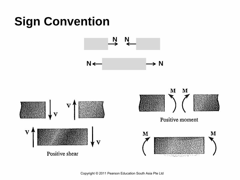
Sign Convention


N N

N N

Example 1:


Example 1: (cont)


This problem can be solved in the most direct manner by

considering segment CB of the beam, since then the support

reactions at A do not have to be computed.

FR=180x6/2= 540 N

At C: 270x6/9= 180 N/m

Try solving this problem using segment AC, by first obtaining the support

reactions at A

Shear and Moment Equations and Daigrams


Equations of V and M as a function of the position x

along the beam’s axis is often needed to find the

maximum values of these loads.

Section the beam at an arbitrary distance x from a

referance point (usually left end point)

V and M functions change at points where a distributed

load changes or where concentrated forces or couple

moments are applied.

Functions must be determined for each section.

Diagrams are helpfull to visualize the change in internal

loads and to decide the important sections.

SHEAR AND MOMENT DIAGRAMS


• Shear is obtained by summing forces

perpendicular to the beam’s axis

up to the end of the segment.

• Moment is obtained by

summing moments about

the end of the segment.

• Note the sign conventions are

opposite when the summing

processes are carried out with

opposite direction. (from left to right vs from right to left)

Please refer to the website for the animation: Shear and Moment Diagrams

Procedure for Analysis


Determine support reactions.

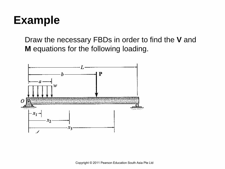
Example


Draw the necessary FBDs in order to find the V and

M equations for the following loading.

FBDs


a<x<b

v

x

N

b<x<c

v

x

N

0<x<a

v

x

N

EXAMPLE 1


Draw the shear and moment diagrams for the beam shown in

Fig. 6–4a.

EXAMPLE 1 (cont.)


Solution

The support reactions are shown in Fig. 6–4c.

Applying the two equations of equilibrium yields

2 2

022

;0

1 2

02

;0

2xLxw

M

Mx

wxxwL

M

xL

wV

VwxwL

Fy

EXAMPLE 1 (cont.)


Solution

The point of zero shear can be found from Eq. 1:

2

02

Lx

xL

wV

8222

22

max

wLLLL

wM

From the moment diagram, this value of x represents the point on the

beam where the maximum moment occurs.

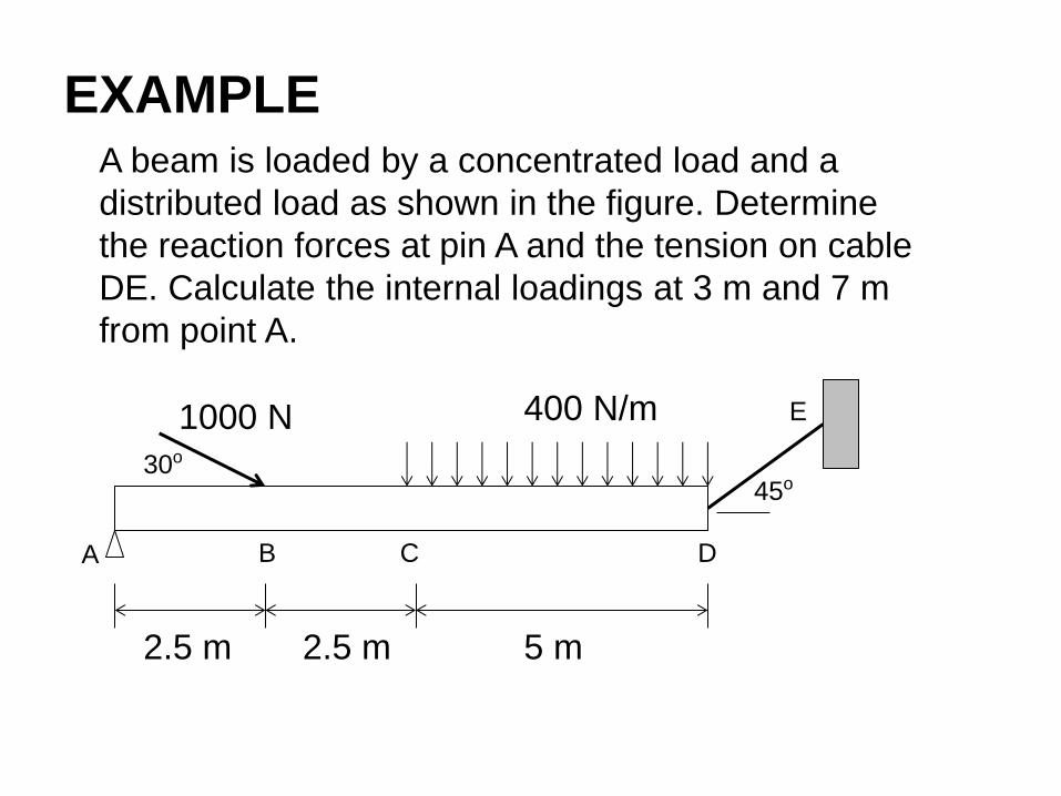
EXAMPLE A beam is loaded by a concentrated load and a

distributed load as shown in the figure. Determine

the reaction forces at pin A and the tension on cable

DE. Calculate the internal loadings at 3 m and 7 m

from point A.

400 N/m 1000 N

A B C D

E

2.5 m 2.5 m 5 m

30o

45o

SOLUTION

0 AM

FBD 2000 N 1000 N

Ax B C D

2.5 m 2.5 m 5 m

T

Ay

30o

45o

1000.sin30.2.5 + 2000.7.5 - T.sin45.10=0 T=2298 N

0 xF

Ax+1000cos30+2300cos45=0 Ax=-2491 N

0 yF

Ay-1000sin30+2300sin45-2000=0 Ay=875 N

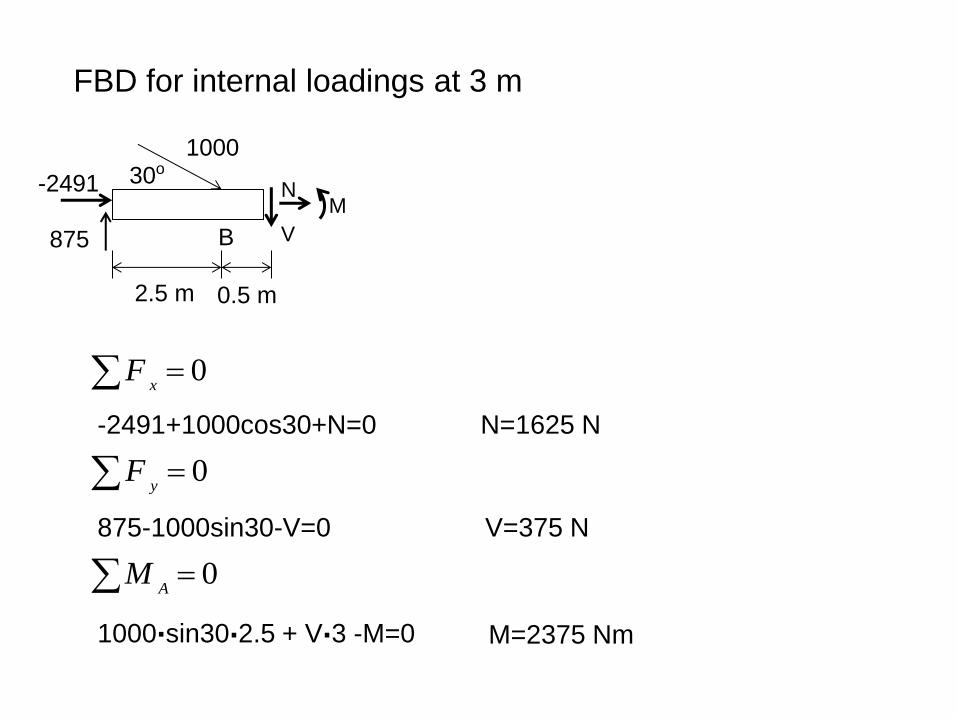
FBD for internal loadings at 3 m

1000

-2491

B

2.5 m 0.5 m

875

30o

M

V

N

0 AM

1000.sin30.2.5 + V.3 -M=0 M=2375 Nm

0 xF

-2491+1000cos30+N=0 N=1625 N

0 yF

875-1000sin30-V=0 V=375 N

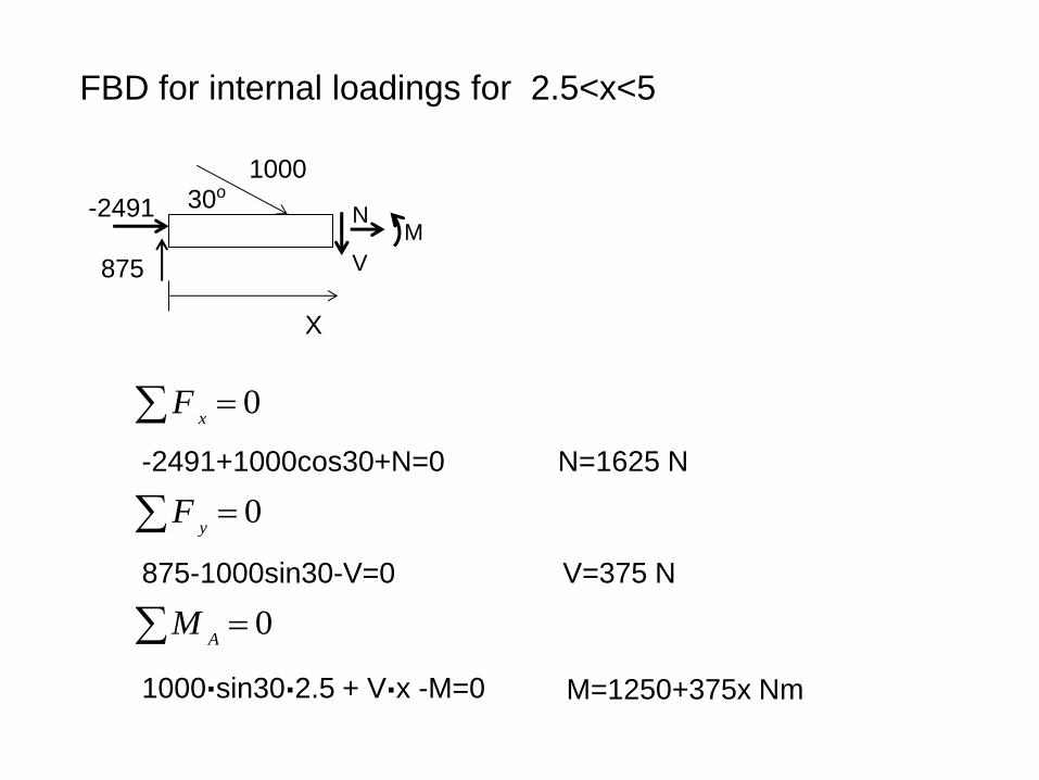
FBD for internal loadings at 7 m

0 AM

1000.sin30.2.5 +800.6+ V.7 -M=0 M=3075 Nm

-2491+1000cos30+N=0 N=1625 N

0 yF

875-1000sin30-800-V=0 V=-425 N

400N/m.2m=800N

1000 N

B C

2.5 m 2.5 m

30o

2 m

M

V

N -2491

875

0 xF

FBD for internal loadings for 0<x<2.5

-2491

X

875

M

V

N

0 AM

V.x -M=0 M=875x Nm

0 xF

-2491+N=0 N=2491 N

0 yF

875-V=0 V=875 N

1000

-2491

875

30o

M

V

N

FBD for internal loadings for 2.5<x<5

X

0 AM

1000.sin30.2.5 + V.x -M=0 M=1250+375x Nm

0 xF

-2491+1000cos30+N=0 N=1625 N

0 yF

875-1000sin30-V=0 V=375 N

400N/m.(x-5) m

1000 N

C

30o

M

V

N -2491

875

X

FBD for internal loadings for 5<x<10

0 AM

1000.sin30.2.5 +400(x-5).[5+(x-5)/2]+ V.x -M=0

-2491+1000cos30+N=0 N=1625 N

0 yF

875-1000sin30-400(x-5)-V=0 V=2375-400x N

0 xF

M=-3750+2375x-200x2

Internal Loadings Diagrams

V (N)

x

875

2.5

10

5

375

-1625

N (N)

x

2491

1625

2.5 10

M (Nm)

x

2188

2.5 10 5

3125 3300

0<x<2.5

M=875x V=875 N=2491

2.5<x<5

M=1250+375x N=1625 V=375

N=1625 V=2375-400x

M=-3750+2375x-200x2

5<x<10

Integration Method

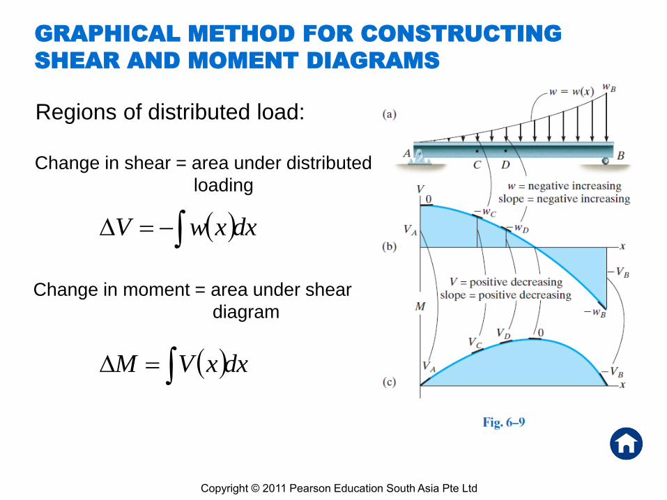
GRAPHICAL METHOD FOR CONSTRUCTING

SHEAR AND MOMENT DIAGRAMS


Regions of distributed load:

dxxwV

dxxVM

Change in moment = area under shear

diagram

Change in shear = area under distributed

loading


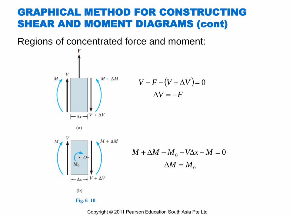
Regions of concentrated force and moment:

FV

VVFV

0

0

0

0

MM

MxVMMM

GRAPHICAL METHOD FOR CONSTRUCTING

SHEAR AND MOMENT DIAGRAMS (cont)

EXAMPLE 2


Draw the shear and moment diagrams for the beam shown in

Fig. 6–12a.

EXAMPLE 2 (cont.)


• The reactions are shown on the

free-body diagram in Fig. 6–12b.

• The shear at each end is plotted first,

Fig. 6–12c. Since there is no

distributed load on the beam,

the shear diagram has zero slope

and is therefore a horizontal line.

Solution

EXAMPLE 2 (cont.)


• The moment is zero at each end,

Fig. 6–12d. The moment diagram

has a constant negative slope of

-M0/2L since this is the shear in the

beam at each point. Note that the

couple moment causes a jump in the

moment diagram at the beam’s

center, but it does not affect the

shear diagram at this point.

Solution

EXAMPLE 3


Draw the shear and moment diagrams for each of the beams

shown in Figs. 6–13a and 6–14a.

EXAMPLE 3 (cont)


Solution

internal loading 7 - gebze technical universityanibal.gyte.edu.tr/.../downloads/chapter-7.pdfexample...

Documents