internal generation of waves for time-dependent mild...

Ž .Coastal Engineering 34 1998 35–57

Internal generation of waves for time-dependentmild-slope equations

Changhoon Lee a,), Kyung Doug Suh b

a Coastal and Harbour Engineering DiÕision, Korea Ocean Research and DeÕelopment Institute, Ansan P.O.Box 29, Seoul 425-600, South Korea

b Department of CiÕil Engineering, Seoul National UniÕersity, Seoul 151-742, South Korea

Received 7 May 1996; revised 20 November 1997; accepted 27 January 1998

Abstract

A technique for internal generation of waves is studied for two time-dependent mild-slopewequation models developed by Copeland Copeland, G.J.M., 1985. A practical alternative to the

x wmild-slope wave equation. Coastal Eng., 9, pp. 125–149 and Radder and Dingemans Radder,A.C., Dingemans, M.W., 1985. Canonical equations for almost periodic, weakly nonlinear gravity

xwaves. Wave Motion, 7, pp. 473–485 . For the Radder and Dingemans’ equations, desired energyof incident waves could not be obtained from the viewpoint of mass transport which hassuccessfully been used for the Boussinesq equations and the Copeland equations by Larsen and

wDancy Larsen, J., Dancy, H., 1983. Open boundaries in short wave simulations—a new approach.x wCoastal Eng., 7, pp. 285–297 and Madsen and Larsen Madsen, P.A., Larsen, J., 1987. An

xefficient finite-difference approach to the mild-slope equation. Coastal Eng., 11, pp. 329–351 ,respectively. However, for both of the Copeland’s and Radder and Dingemans’ models, desiredenergy of incident waves could be obtained from the viewpoint of energy transport. Using theviewpoint of energy transport in the Radder and Dingemans equations, which treat random wavesof narrow frequency band properly, we could successfully generate not only monochromaticwaves but also directional random waves. q 1998 Elsevier Science B.V. All rights reserved.

Keywords: Time-dependent mild-slope equations; Numerical wave generation; Energy transport

1. Introduction

The prediction of the transformation of water waves is important to coastal engineerswho utilize and protect coastal regions by designing, constructing and maintaining

) Corresponding author. Fax: q82-345-408-5823, e-mail: [email protected].

0378-3839r98r$19.00 q 1998 Elsevier Science B.V. All rights reserved.Ž .PII: S0378-3839 98 00012-X

( )C. Lee, K.D. SuhrCoastal Engineering 34 1998 35–5736

breakwaters, harbors, beach resorts, etc. Among the mathematical models, the ellipticŽ .mild-slope equation developed by Berkhoff 1972 is known as a linear model which

predicts such transformation of regular waves as refraction, diffraction, shoaling, andreflection. In solving the elliptic equation, all the boundary conditions need to bespecified, and thus, the solution of a matrix is necessary, which usually requires a lot ofcomputational time. As an alternative to the elliptic mild-slope equation, its parabolicapproximations have also been used to solve the water wave transformation efficiently.But, in the case where significant wave reflection occurs or wave directions are largelydeviated away from the presumed direction, the solution by the parabolic equation yieldserrors. As another alternative, hyperbolic equations have also been used with the sameaccuracy but with less computational time compared to the elliptic equation.

Ž .Smith and Sprinks 1975 derived a hyperbolic time-dependent mild-slope equationŽ .using the Green’s second identity, and Radder and Dingemans 1985 provided a

canonical form of the time-dependent mild-slope equations based on the Hamiltoniantheory of surface waves. The Radder and Dingemans equations, which includes twovariables of the water surface elevation and the velocity potential at the free surface, canbe reduced to the Smith and Sprinks equation by eliminating the surface elevation. For

Ž .the waves propagating on currents, Booij 1981 derived a canonical form of theŽ .time-dependent mild-slope equations using the Lagrangian formula and Kirby 1984

corrected some errors in the Booij equations. Without current, these equations reduce tothe equations of Radder and Dingemans. The equations of Kirby, which include twovariables of the surface elevation and the velocity potential at the free surface, can alsobe reduced to one equation by eliminating the surface elevation. This equation in turn,

Ž .without current, reduces to the Smith and Sprinks equation. Nishimura et al. 1983derived time-dependent mild-slope equations by vertically integrating the continuity and

Ž .momentum equations for linear waves. Copeland 1985 also derived similar time-de-pendent equations from the Smith and Sprinks equation using the characteristics oflinear waves and the definition of a volume flux. The two models of Nishimura et al.and Copeland are mathematically equivalent to each other and also to the Berkhoff’s

Ž .elliptic model. Kubo et al. 1992 derived a time-dependent mild-slope equation usingthe Taylor series expansion technique for waves with local frequencies different from

Ž .the carrier frequency. Lee and Kirby 1994 found that the models of Smith and Sprinks,Radder and Dingemans, and Kubo et al. could be applied to narrow frequency-banded

Ž . Žrandom waves with accuracy of O Dk Dkskyk, k is the local wavenumber and k. Ž .is the carrier wavenumber . Recently, Lee 1994 derived two time-dependent equation

ŽŽ .2 .models for random waves with accuracy of O Dk by adding a correction term to theSmith and Sprinks’ and Kubo et al.’s models, respectively.

In order to solve the time-dependent mild-slope equations in a region, initial andboundary conditions need to be specified. Usually, all the values at the initial stage are

Ž .set as zero i.e., cold start . Waves can be generated by specifying the values of watersurface elevation, particle velocity, or volume flux as desired at the wave generation lineinside or outside the boundary at each time step. Waves can also be generated by addingthe values with desired wave energy to the computed values at the wave generation lineinside the boundary at each time step. When the former way is used, problems mayoccur because the waves which arrive at the wave generation line from the inside of the

( )C. Lee, K.D. SuhrCoastal Engineering 34 1998 35–57 37

computational domain would be trapped, and thus, cause unwanted addition of waveenergy and distortion of wave phase inside the domain. However, the latter way does notgive rise to such problems because it permits the waves to pass freely across the wavegeneration line while desired wave energy is generated at the line. The latter way,so-called internal generation of waves, has been used by several coastal engineersŽLarsen and Dancy, 1983 for the Boussinesq equations of Peregrine, 1967; Madsen and

.Larsen, 1987 and Yoon et al., 1996 for the Copeland equations . They have used theviewpoint of mass transport in which the velocity of disturbances caused by the incidentwave is the phase speed.

In this study, we apply the internal generation of waves to two typical time-dependentŽ .mild-slope equation models developed by Copeland 1985 and Radder and Dingemans

Ž .1985 , respectively, and find that the velocity of disturbances caused by the incidentwave can be obtained properly from the viewpoint of energy transport. In Section 2, theinternal generation of waves from the viewpoint of mass transport is made for bothCopeland’s and Radder and Dingemans’ models. In Section 3, the generation of wavesby the viewpoint of energy transport is considered and the energy velocity is obtainedusing the geometric optics approach. In Section 4.1, the finite difference methods usedare described. In Section 4.2, from the viewpoints of both mass transport and energytransport, uni-directional monochromatic waves are internally generated for the twomodels. In Sections 4.3, 4.4 and 4.5, from the viewpoint of energy transport, uni-direc-tional random waves, multi-directional monochromatic waves, and multi-directionalrandom waves are generated for the Radder and Dingemans model. In Section 5,summary and discussions are presented.

2. Internal generation of waves from the viewpoint of mass transport

Ž .The Copeland 1985 equations are given by:

Eh Cq =PQs0 1Ž .

E t Cg

E QqCC =hs0 2Ž .gE t

where = is the horizontal gradient operator, C and C are the phase speed and groupg

velocity, respectively, of a wave with carrier angular frequency v and wavenumber k, h

is the water surface elevation, and Q is a vertically integrated function of particlevelocity given by:

QsC h . 3Ž .g

The wavenumber k is determined from the linear dispersion relation given by:

2v sgk tanh kh 4Ž .


where g is the acceleration due to gravity and h is the water depth. Elimination of QŽ . Ž .from Eqs. 1 and 2 yields:

2E h Cy =P CC =h s0. 5Ž .ž /g2E t Cg

Ž .The Radder and Dingemans 1985 equations are given by:

2 2Eh CC v yk CCg g˜ ˜ ˜sy=P =f q fsF f 6Ž .Ž .ž /E t g g

˜Efsygh 7Ž .

E t˜where f is the velocity potential at mean water level which is related to h by:

igf̃sy h 8Ž .

v

' Ž . Ž .where is y1 . Elimination of h from Eqs. 6 and 7 yields the Smith and Sprinks˜equation in terms of f given by:

2 ˜E f2 2˜ ˜y=P CC =f q v yk CC fs0. 9Ž .ž / ž /g g2E t

For later use, we express the preceding equation in terms of h. Because this equation is˜ Ž . Ž .linear and f and h are linearly related as in Eq. 8 , Eq. 9 can be written as:

E 2h2 2y=P CC =h q v yk CC hs0. 10Ž .ž / ž /g g2E t

Ž .Larsen and Dancy 1983 used the technique of internal generation of waves in theŽ .Boussinesq equations of Peregrine 1967 from the viewpoint of mass transport. Their

principle on wave generation is as follows. When the incident wave of speed C and theelevation h I propagates at an angle u from the x-axis, the speed to the x-axis would beC cos u . Let D x and D y be the grid spacing in the x- and y-directions, respectively,and the line of wave generation, l, be parallel to the y-axis. Then, the distance between

Isuccessive grid points on l is D y and the volume flux across l is h C cos u in bothpositive and negative x-directions. Since a grid point covers an area of D xD y, thesurface elevation to be added to h at each grid point of l is:

CD tIh)s2h cosu . 11Ž .

D xŽ .Madsen and Larsen 1987 also used the internal generation of waves in the modified

Copeland equations where the time-harmonics terms are extracted to give:

C Eh Cˆg g ˆq iv hq=PQsSS 12Ž .ˆE tC C

ˆC E Q Cg g 2ˆq iv QqC =hs0 13Ž .ˆgE tC C


where:

hshei v t 14Ž .ˆˆ i v tQsQe 15Ž .

and the source term SS is:

CgSSs cosu . 16Ž .

D x

Ž . Ž . Ž . Ž .When Eqs. 12 and 13 are recovered to the original Eqs. 1 and 2 , the sourceŽ .term SS would be equal to h) in Eq. 11 . This means that the wave generation with

the source term in the modified Copeland equations is made from the viewpoint of massŽ .transport. Yoon et al. 1996 also used the internal generation of waves in Copeland

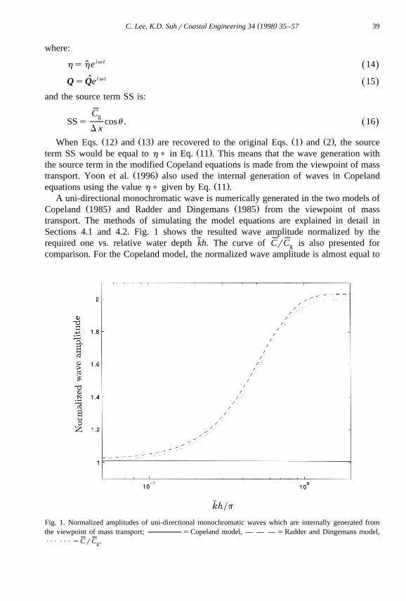
Ž .equations using the value h) given by Eq. 11 .A uni-directional monochromatic wave is numerically generated in the two models of

Ž . Ž .Copeland 1985 and Radder and Dingemans 1985 from the viewpoint of masstransport. The methods of simulating the model equations are explained in detail inSections 4.1 and 4.2. Fig. 1 shows the resulted wave amplitude normalized by therequired one vs. relative water depth kh. The curve of CrC is also presented forg

comparison. For the Copeland model, the normalized wave amplitude is almost equal to

Fig. 1. Normalized amplitudes of uni-directional monochromatic waves which are internally generated fromthe viewpoint of mass transport; sCopeland model, — — — sRadder and Dingemans model,PPP PPP sCrC .g


unity in whole water depth. However, for the Radder and Dingemans model, thenormalized wave amplitude is close to the curve of CrC which is almost equal to unityg

in shallow water but greater than unity in deep and intermediate-depth waters. Thisimplies that there is a limitation in using the viewpoint of mass transport for internalgeneration of waves in the Radder and Dingemans model.

3. Internal generation of waves from the viewpoint of energy transport

The time-dependent wave equation models predict the evolution of wave energy aswell as the change of wave phase. When the water surface elevation of incident waves isadded to the computed one at each time step at the wave generation line, there occurs anevolution of wave energy as well as a change in wave phase. The evolution of waveenergy can be predicted by the transport equation for wave energy. That is, the velocityof disturbances caused by the incident wave is the energy velocity C and the value h)e

added to the surface elevation at each time step at the wave generation line would be:

C D teIh)s2h cosu . 17Ž .D x

Ž . Ž .The difference of Eq. 17 from Eq. 11 is that the energy velocity is used instead of thephase speed for the propagation of disturbances caused by the incident wave.

The energy velocity for a time-dependent model can be obtained analytically usingthe geometric optics approach. When surface waves propagate on a constant waterdepth, the geometric optics approach yields the eikonal equation and the transportequation for wave energy, and the energy velocity can be obtained from these twoequations. The water surface elevation can be expressed as:

hsA x , y ,t e ic 18Ž . Ž .where the wave amplitude A modulates in time and space, and the phase function c hasthe following relations with the local wavenumber vector k and angular frequency v:

Ecks=c , vsy . 19Ž .

E t

Ž . Ž .Substitution of Eq. 18 into the Copeland equation, Eq. 5 yields:

2E A E A C2y2 iv yv Ay =P CC =A q i=P kCC Až / ž /g g2 E tE t Cg

2qikCC P=Ayk CC A s0. 20Ž .g g

Ž .The terms in the real part of Eq. 20 yield the eikonal equation given by:

2 22 =P CC =Ak v 1 E Až /gs q y 21Ž .2 2ž /ž / 2v v A E tk k CC Ag


where the second and third terms in the right-hand side are negligibly small compared toother terms. Neglecting these terms yields:

k vs . 22Ž .

vk

Ž .The terms in the imaginary part of Eq. 20 multiplied by A yield the transport equationfor wave energy given by:

2 2E A k C2q P=A s0 23Ž .

E t k C

Ž .where, based on the definition of CsCkrk and the use of Eq. 22 , the energy velocityis given by:

2k CC s sC . 24Ž .e k C

Ž . Ž .Substitution of Eq. 18 into the Smith and Sprinks Eq. 10 yields:

E 2A E A2y2 iv yv Ay=P CC =A y i=P kCC Až / ž /g g2 E tE t

2 2 2y ikCC P=Aqk CC Aq v yk CC As0. 25Ž .ž /g g g

Ž .The terms in the real part of Eq. 25 yield the eikonal equation given by:

2 22 =P CC =Ak C v 1 E Až /gs1q y1 q y 26Ž .2 2ž /ž / 2v v A E tk C k CC Ag g

where the second and third terms in the right-hand side are again negligibly smallcompared to other terms. Neglecting these terms yields:

2k C vs 1q y1 . 27Ž .) ž /vk Cg

Ž .The terms in the imaginary part of Eq. 25 multiplied by A yield the transport equationfor wave energy given by:

2E A k CCg 2q P=A s0 28Ž .E t k C

Ž .where, based on the definition of C sC krk and the use of Eq. 27 , the energyg g

velocity is given by:

2k CC v C vgC s sC 1q y1 . 29Ž .e g ) ž /k C v vCg

It should be noted that the energy velocity is not a physically true value but a valuereduced in the mathematical model. In the Copeland model, the energy velocity is the


Ž .phase speed, as shown in Eq. 24 . In fact, the Copeland model cannot predict the groupŽ .behavior of random waves Kirby et al., 1992 . That is, in the Copeland model, the use

of the viewpoint of energy transport in internal wave generation gives the same result asthat obtained from the viewpoint of mass transport. In the Smith and Sprinks model, theenergy velocity is the group velocity C for regular waves with vrvs1, as shown ing

Ž .Eq. 29 .

4. Numerical simulation

In this section, the internal wave generation technique is numerically tested. First,from the viewpoints of both mass transport and energy transport, uni-directional

Ž .monochromatic waves are generated in the two models of Copeland 1985 and RadderŽ .and Dingemans 1985 . The two different viewpoints produce the same results for the

Copeland model. For the Radder and Dingemans model, however, it is shown that theviewpoint of energy transport works well in deep to shallow waters while that of masstransport gives correct results only in shallow water. Further tests on the Radder andDingemans model are then made for uni-directional random waves, multi-directionalmonochromatic waves, and multi-directional random waves by using the viewpoint ofenergy transport.

4.1. Finite difference method

Ž .Sponge layers are placed at the outside boundaries see Figs. 2 and 8 to minimizewave reflection from the boundaries by dissipating wave energy inside the sponge

Ž .layers. Thus, for the Copeland model, Eq. 2 is modified as:

E QqCC =hqv D Qs0, 30Ž .g sE t

Ž .and, for the Radder and Dingemans model, Eq. 7 is modified as:

˜Ef˜ ˜syghyv D fsG h ,f . 31Ž .Ž .sE t

The damping coefficient D is given by:s

0, outside sponge layer°~exp drS y1Ž .D s 32Ž .s , inside sponge layer¢ exp 1 y1Ž .

where d is the distance from the starting point of the sponge layer and S is the thicknessof the sponge layer.


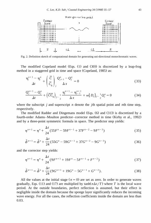
Fig. 2. Definition sketch of computational domain for generating uni-directional monochromatic waves.

Ž Ž . Ž ..The modified Copeland model Eqs. 1 and 30 is discretized by a leap-frogŽ .method in a staggered grid in time and space Copeland, 1985 as:

nq1 n n nh yh C Q yQj j jq1 jq s0 33Ž .ž /Dt D xCg j

Qnq1 yQn h nq1 yh nq1j j j jy1 n11 w xq CC qv D Q s0 34Ž .jyž /g s jjy 2Dt D x2

where the subscript j and superscript n denote the jth spatial point and nth time step,respectively.

Ž Ž . Ž ..The modified Radder and Dingemans model Eqs. 6 and 31 is discretized by aŽ .fourth-order Adams–Moulton predictor–corrector method in time Kirby et al., 1992

and by a three-point symmetric formula in space. The predictor step yields:

D tnq1 n n ny1 ny2 ny3h sh q 55F y59F q37F y9F 35Ž . Ž .

24

D tnq1 n n ny1 ny2 ny3˜ ˜f sf q 55G y59G q37G y9G 36Ž . Ž .

24

and the corrector step yields:

D tnq1 n nq1 n ny1 ny2h sh q 9F q19F y5F qF 37Ž . Ž .

24

D tnq1 n nq1 n ny1 ny2˜ ˜f sf q 9G q19G y5G qG . 38Ž . Ž .

24

Ž .All the values at the initial stage ns0 are set as zero. In order to generate wavesŽ . Ž . Ž .gradually, Eqs. 11 and 17 are multiplied by tanh nD trT where T is the local wave

period. At the outside boundaries, perfect reflection is assumed, but their effect isnegligible inside the domain because the sponge layer significantly reduces the incomingwave energy. For all the cases, the reflection coefficients inside the domain are less than0.03.


4.2. Uni-directional monochromatic waÕes

For uni-directional monochromatic waves, the computational domain consists of anŽ .inner domain of 8 L where L is the local wavelength and two sponge layers with the

Ž .thickness Ss3L at the outside boundaries see Fig. 2 . The wave generation point isplaced at the central point of the inner domain. The grid spacing D x is chosen so thatLrD xs20 and a spatial resolution is guaranteed. The time step D t is chosen so that theCourant number C sC D trD xs0.1 and a stable solution is guaranteed.r e

First, we numerically generate uni-directional monochromatic waves from the view-points of both mass transport and energy transport. Tests are made for various values ofrelative water depth. For the Copeland model, without showing the results, we justmention that the result from the viewpoint of energy transport is the same as that from

Ž .the viewpoint of mass transport as shown in Fig. 1 , both of them being close to therequired value. This is because the energy velocity is equivalent to the phase speed inthe Copeland model. Fig. 3 shows the wave amplitude normalized with respect to therequired one for the Radder and Dingemans model based on the viewpoints of both masstransport and energy transport. The viewpoint of energy transport predicts the waveamplitude correctly for all depths while that of mass transport gives correct results onlyin shallow water where the energy velocity is the same as the phase speed.

Fig. 3. Normalized amplitudes of uni-directional monochromatic waves which are internally generated inRadder and Dingemans model; senergy transport, — — — smass transport.


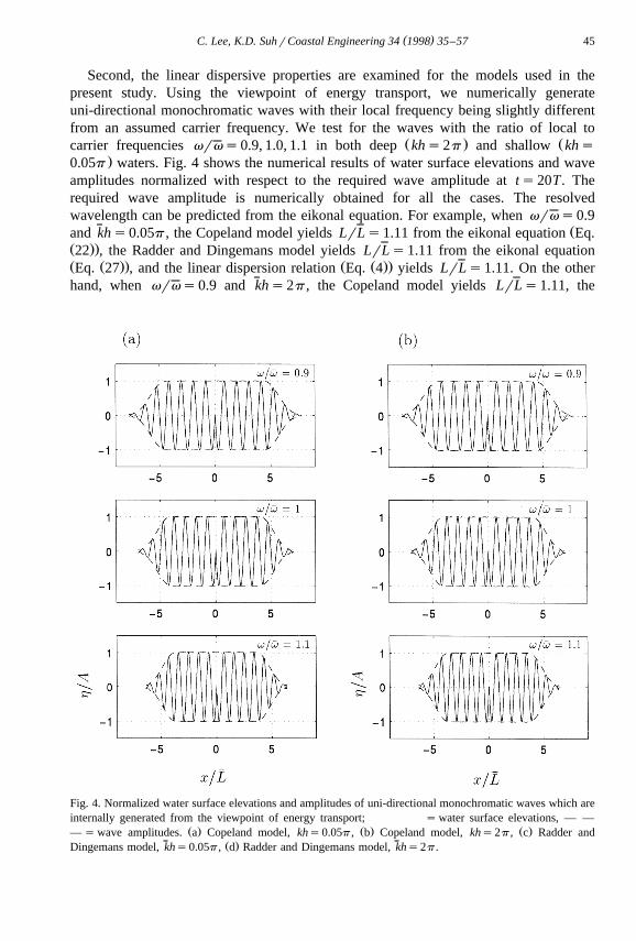
Second, the linear dispersive properties are examined for the models used in thepresent study. Using the viewpoint of energy transport, we numerically generateuni-directional monochromatic waves with their local frequency being slightly differentfrom an assumed carrier frequency. We test for the waves with the ratio of local to

Ž . Žcarrier frequencies vrvs0.9, 1.0, 1.1 in both deep khs2p and shallow khs.0.05p waters. Fig. 4 shows the numerical results of water surface elevations and wave

amplitudes normalized with respect to the required wave amplitude at ts20T. Therequired wave amplitude is numerically obtained for all the cases. The resolvedwavelength can be predicted from the eikonal equation. For example, when vrvs0.9

Žand khs0.05p , the Copeland model yields LrLs1.11 from the eikonal equation Eq.Ž ..22 , the Radder and Dingemans model yields LrLs1.11 from the eikonal equationŽ Ž .. Ž Ž ..Eq. 27 , and the linear dispersion relation Eq. 4 yields LrLs1.11. On the otherhand, when vrvs0.9 and khs2p , the Copeland model yields LrLs1.11, the

Fig. 4. Normalized water surface elevations and amplitudes of uni-directional monochromatic waves which areinternally generated from the viewpoint of energy transport; s water surface elevations, — —

Ž . Ž . Ž .— s wave amplitudes. a Copeland model, khs0.05p , b Copeland model, khs2p , c Radder andŽ .Dingemans model, khs0.05p , d Radder and Dingemans model, khs2p .


Ž .Fig. 4 continued .

Radder and Dingemans model yields LrLs1.27, and the linear dispersion relationyields LrLs1.23. The Copeland model cannot produce the behavior of random waves

Ž .properly, thus yields 10% error of wavelength in deep water for the case of vyv rv

sy0.1. But, the Radder and Dingemans model yields only 3% error for that case.Fig. 4 also shows that for the Radder and Dingemans model, the resolved wave

amplitude fluctuates around the exact solution. This is because the standard discretiza-tion is made across the wave generation point and the distortion of the solution isresulted. This phenomenon is not observed for the Copeland model because variables h

and Q in the model are placed at the staggered grids in time and space. That is, if astaggered grid system was used in discretizing the Radder and Dingemans equations, thefluctuation of wave amplitudes could be avoided.

4.3. Uni-directional random waÕes

We consider the case of uni-directional random waves. The wave amplitude of thecomponent wave with frequency f for uni-directional random waves is given by Ai i


Ž .s 2S f D f . The frequency spectrum of incident waves, S f , is taken as the TMA( Ž .i i

spectrum which can be applied in shallow water:

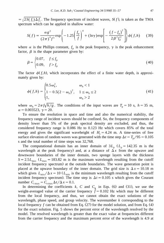
242 ° ¶a g f fy fŽ .p p~ •S f s exp y1.25 q lng exp y f f ,h 39Ž . Ž . Ž . Ž .4 2 25 ž /¢ ßf 2b f2p fŽ . p

where a is the Phillips constant, f is the peak frequency, g is the peak enhancementp

factor, b is the shape parameter given by:

0.07, fF fpbs 40Ž .½0.09, f) fp

Ž .The factor f f ,h , which incorporates the effect of a finite water depth, is approxi-mately given by:

° 20.5v , v -1h h

2~f f ,h s 41Ž . Ž .1y0.5 2yv , 1Fv F2Ž .h h¢1, v )2h

'where v s2p f hrg . The conditions of the input waves are T s10 s, hs35 m,h p

as0.003523, gs20.To ensure the resolution in space and time and also the numerical stability, the

frequency range of incident waves should be confined. So, the frequency components ofdensity lower than 5% of the peak spectral density are excluded, and thus, theconsidered frequency range is 0.086 Hz to 0.123 Hz which covers 85% of the totalenergy and gives the significant waveheight of H s4.24 m. A time-series of frees

surface elevation of random waves was generated with the time step D tsT r95s0.105p

s and the total number of time steps was 32,768.ŽThe computational domain has an inner domain of 3L L s142.35 m is thep p

.wavelength at the peak frequency and, at a distance of D x from the upwave anddownwave boundaries of the inner domain, two sponge layers with the thickness

ŽSs2.5L L s183.82 m is the maximum wavelength resulting from the cutoffmax max.incident frequency spectrum at the outside boundaries. The wave generation point is

placed at the upwave boundary of the inner domain. The grid size is D xs10.18 mŽwhich gives L rD xs10 L is the minimum wavelength resulting from the cutoffmin min.incident frequency spectrum . The time step is D ts0.105 s which gives the Courant

number C sC D trD xs0.1.r max e maxŽ . Ž .In determining the coefficients k, C and C in Eqs. 6 and 31 , we use theg

weight-averaged value of the carrier frequency fs0.102 Hz which may be differentfrom the local frequency, and thus, we cannot obtain the exact solutions of thewavelength, phase speed, and group velocity. The wavenumber k corresponding to the

Ž . Ž .local frequency f can be obtained from Eq. 27 for the model solution, and from Eq. 4for the exact solution. Fig. 5 shows the percent error of the wavelength resolved by themodel. The resolved wavelength is greater than the exact value at frequencies differentfrom the carrier frequency and the maximum percent error of the wavelength is 4.9 at


Fig. 5. Percent error of the resolved wavelength compared to the exact solution.

fs0.123 Hz. However, the spectral densities at frequencies with larger errors arenegligibly small compared to that around the carrier frequency, and thus, the wavelengthresolved by the model is almost the same as the exact one. This is proven by Fig. 6which shows the comparison of resolved water surface elevations and the correspondingexact solutions at ts10T .p

The water surface elevation was recorded at a distance of L downwave from thep

wave generation point. In order to permit the slower-travelling high-frequency compo-nent waves to reach to the point of wave recording, the surface elevation was recordedfrom 10T to 347.81T with the sampling interval of T r24.25 so that the total numberp p p

of sample was 8192. In the spectral analysis of the data, the smoothing techniquesŽ .presented in Otnes and Enochson 1978 were used. The 8192 data points were

Fig. 6. Water surface elevations of uni-directional random waves at ts10T ; snumericalp

solution, — — — sexact solution.


Fig. 7. Frequency spectrum of uni-directional random waves; ssimulated, — — — s target.

processed in four segments of 2048 points per segment. These segments overlapped by50% for smoother and statistically more significant spectral estimates. The raw spectrawere then ensemble-averaged. Further smoothing was made by band-averaging over five

Fig. 8. Definition sketch of computational domain for internally generating multi-directional monochromaticwaves.


neighboring frequency bands. The total number of degrees of freedom is about 27 forfinal spectra. Fig. 7 shows that the power spectra of numerically simulated water surfaceelevation is almost the same as the target spectra.

4.4. Multi-directional monochromatic waÕes

In order to generate multi-directional waves in a two-dimensional domain, we putŽ . Žthree wave generation lines, one WGL 1 along the y-direction and the others WGL 2

. Ž .and WGL 3 along the x-direction see Fig. 8 . The computational domain consists of

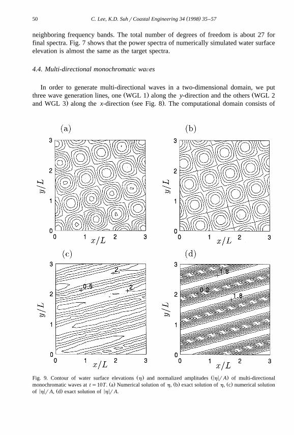
Ž . Ž < < .Fig. 9. Contour of water surface elevations h and normalized amplitudes h r A of multi-directionalŽ . Ž . Ž .monochromatic waves at ts10T. a Numerical solution of h, b exact solution of h, c numerical solution

< < Ž . < <of h r A, d exact solution of h r A.


the inner domain of 3L=3L and sponge layers with the thickness Ss2.5L at fouroutside boundaries. WGL 2 and WGL 3 start at a distance of D x away from the upwave

Ž Ž . Ž . .sponge layer i.e., 0, 0 and 0, 3L , respectively and end at the downwave boundaryŽ Ž . Ž . .points i.e., 3LqS, 0 and 3LqS, 3L , respectively . In the case of normal incidence

Ž . Žus08 , only WGL 1 operates and it is placed from the rightwave boundary 0,. Ž .yD yyS to the leftwave boundary 0, 3LqD yqS . In the case of positive waveŽ .direction u)08 , WGL 1 and WGL 2 operate and WGL 1 is placed from the starting

Ž . Ž .point of WGL 2 0, 0 to the leftwave boundary 0, 3LqD yqS . In the case ofŽ .negative wave direction u -08 , WGL 1 and WGL 3 operate and WGL 1 is placed

Ž . Ž .from the rightwave boundary 0, yD yyS to the starting point of WGL 3 0, 3L . Thewave generation lines WGL 1 to 3 operate simultaneously at each time step in order toget efficient computational time. The value h) added to the water surface elevations atWGL 1 at each time step is given by:

C Dteih)s 2 A cos k x cosu qk y sinu yv tqe cosu 42Ž .Ž .ÝÝ i , j i j i j i i , j j

Dxi j

and the value h) added to the water surface elevations at WGL 2 or WGL 3 at eachtime step is given by:

C D tei< <h)s 2 A cos k x cosu qk y sinu yv tqe sin u . 43Ž .Ž .ÝÝ i , j i j i j i i , j j

D yi j

Ž . Ž .In Eqs. 42 and 43 , the subscripts i and j denote the components of differentfrequency and direction, respectively, A is the amplitude of each wave component,i , j

and e is the phase angle which, for random waves, is randomly but uniformlyi , j

distributed between 0 and 2p .We consider the case of two monochromatic waves propagating in different direc-

tions with the same frequency and amplitude. The conditions of the incident waves areTs10 s, hs35 m, A sA s3.5 m, e se s08, u s608, u sy308. The grid size1 2 1 2 1 2

is D xsD ys14.25 m which gives LrD xsLrD ys10. The time step is D ts0.15 swhich gives the Courant number C sC D trD xs0.1.r e

Fig. 9 shows the comparison of numerical solutions of water surface elevation andnormalized wave amplitude against the corresponding exact solutions at ts10T. Thewave phase of the numerical solution is almost the same as that of the exact solution.The wave amplitude of the numerical solution is a little larger than that of the exactsolution probably because the sponge layer cannot perfectly absorb the wave energy so

Table 1Test conditions of incident multi-directional random waves

Ž . Ž . Ž . Ž . Ž .Case ID T s h m a g u deg s deg u degp m m j

M1 10 35 0.003523 20 0 10 y14, y5, 0, 5, 14M2 10 35 0.003523 20 0 30 y42, y16, 0, 16, 42M3 10 35 0.003523 20 30 10 16, 25, 30, 35, 44M4 10 35 0.003523 20 30 30 y12, 14, 30, 46, 72


that a minor wave reflection occurs. Wave diffraction occurred at the points ofŽdiscontinuity of wave energy such as the boundary points of wave generation lines i.e.,

Ž . Ž ..0, 0 and 0, 3L and the points on WGL 1 located in the sponge layer, and thus,deteriorated the accuracy of the numerical solutions.

4.5. Multi-directional random waÕes

Finally, we consider the case of multi-directional random waves. The frequencyspectrum of the incident waves is the same as that for the uni-directional random waves

Fig. 10. Contour of water surface elevations of multi-directional random waves at ts10T ; spŽ . Ž . Ž . Ž .numerical solution, — — — sexact solution. a M1, b M2, c M3, d M4.


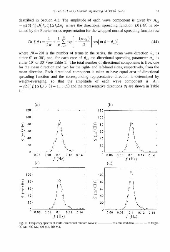
described in Section 4.3. The amplitude of each wave component is given by Ai, j

Ž .s 2S f D f ,u D f Du where the directional spreading function D f ,Q is ob-Ž . Ž .( i i j i j

tained by the Fourier series representation for the wrapped normal spreading function as:

N1 1 nsŽ .mD f ,u s q exp y cos n uyu 44Ž . Ž . Ž .Ý m2p p 2ns1

Ž .where N s20 is the number of terms in the series, the mean wave direction u ism

either 08 or 308, and, for each case of u , the directional spreading parameter s ism mŽ .either 108 or 308 see Table 1 . The total number of directional components is five, one

for the mean direction and two for the right- and left-hand sides, respectively, from themean direction. Each directional component is taken to have equal area of directionalspreading function and the corresponding representative direction is determined byweight-averaging, so that the amplitude of each wave component is Ai, j

Ž .s 2S f D f r5 js1, . . . ,5 and the representative directions u j are shown in Table( Ž .i i

1.

Fig. 11. Frequency spectra of multi-directional random waves; ssimulated data, — — — s target.Ž . Ž . Ž . Ž .a M1, b M2, c M3, d M4.


The computational domain consists of an inner domain of 3L =3L and the spongep p

layers with the thickness Ss2.5L at four outside boundaries. We place three wavemax

generation lines, one at the upwave boundary and two at the right- and left-waveboundaries of the inner domain. The grid size is D xsD ys10.18 m which givesL rD xsL rD ys10. The time step is D ts0.105 s which gives the Courantmin min

number C sC D trD xs0.1.r max e max

Fig. 10 shows the comparison between numerical solutions of water surface elevationand the corresponding exact solutions at ts10T . For all the cases, the wave phase ofp

numerical solutions is almost the same as that of the exact solutions. The minordifferences in wave phase might have resulted from the imperfect absorption of waveenergy in the sponge layer and the diffraction of wave energy at the points of energydiscontinuity.

Ž . ŽThe water surface elevation h and its slopes in the x- and y-directions EhrEx,. Ž . Ž .EhrE y were recorded at the point of x, y s L , 1.5L from 10T to 347.81T withp p p p

the sampling interval of D tsT r24.25 so that the total number of sample was 8192.p

The slope of surface elevation was obtained by discretizing the surface elevations with

Ž . Ž .Fig. 12. Contour of directional spectra of multi-directional random waves. a M1, simulated, b M1, target,Ž . Ž . Ž . Ž . Ž . Ž .c M2, simulated, d M2, target, e M3, simulated, f M3, target, g M4, simulated, h M4, target.


Ž .Fig. 12 continued .

the three-point symmetric formula. Fig. 11 shows that the power spectrum of measuredwater surface elevations is almost the same as the target spectrum for all the casesexcept the case of M4. For the case of M4, the measured power spectrum is somewhatlarger than the target spectrum probably because of imperfect absorption of wave energyin the sponge layer and diffraction of wave energy at the energy discontinuity points.

In order to obtain the directional wave spectrum of the numerically simulated waveŽ . Ž .field, we analyzed the measured surface elevation h and its slopes EhrEx, EhrE y by

Ž .using the maximum entropy principle developed by Kobune and Hashimoto 1986 . TheNewton–Raphson method was used in solving the nonlinear equations which arereduced during the spectral analysis, and the initial guesses for the solution were

Ž .selected as the approximate solutions proposed by Kim et al. 1994 who used theTaylor series technique.

Fig. 12 shows the comparison of the directional spectra of the simulated wave fieldagainst the corresponding target spectra. For all the cases, the mean wave direction wasexactly reproduced as required. The peak spectral density of the simulated data is almostthe same as that of the target spectrum for s s108, but it is somewhat larger than thatm


of the target spectrum for s s308. This is probably because, as directional spreadingm

becomes larger, more wave reflection occurs along the direction normal to the meanwave direction.

5. Conclusions

The internal generation of waves has been studied for two time-dependent mild-slopeŽ . Ž .equations developed by Copeland 1985 and Radder and Dingemans 1985 , respec-

tively. The viewpoints of mass transport and energy transport suggest the use of thephase speed and the energy velocity, respectively, for the velocity of disturbancescaused by the incident waves. It is found that the viewpoint of mass transport, which has

Ž .been used by Larsen and Dancy for the Boussinesq equations of Peregrine 1967 and byMadsen and Larsen for the Copeland equations, cannot properly generate waves for theRadder and Dingemans equations. The time-dependent wave equation models predict theevolution of wave energy as well as the change of wave phase. This implies that theenergy velocity would be the velocity of disturbances caused by the incident waves. Thegeometric optics approach is used to obtain the eikonal equation and the transportequation for wave energy, thus, to get the energy velocity for the time-dependentmodels. In the Copeland model, the energy velocity is equivalent to the phase speed sothat the use of the viewpoint of energy transport in internal wave generation gives thesame result as the use of the viewpoint of mass transport.

Numerical simulations of uni-directional monochromatic waves with various ratios oflocal to carrier frequencies showed that the energy transport is the proper viewpoint ingenerating waves internally in the Radder and Dingemans model. The numericalsimulations also showed that the wavelength that resulted from the model could beexactly predicted from the eikonal equation. Using the Radder and Dingemans modelwhich treats properly the group behavior of random waves of narrow frequency band,we generated successfully uni-directional random waves, multi-directional monochro-matic waves, and multi-directional random waves from the viewpoint of energy trans-port.

It has been shown that the viewpoint of energy transport works correctly for internalŽ .generation of waves in the models of Copeland 1985 and Radder and Dingemans

Ž .1985 . However, it is not certain whether this applies to other time-dependent waveequations such as the Boussinesq equations. The viewpoint of energy transport results in

w Ž .2 � Ž .24xC sC 1y kh r 3q kh for the Peregrine’s Boussinesq equations, which is theeŽ .same as the group velocity, C , obtained by Madsen et al. 1991 . This is in contrast tog

Ž .Larsen and Dancy 1983 , who showed that the source formulation of internal wavegeneration should be expressed in terms of the phase velocity, C, rather than the groupvelocity, C . This conflict may become significant if the waves are generated ing

intermediate-depth or deep water. Recently, several researchers have extended theŽapplicable range of the Boussinesq equations to deeper waters Madsen and Sorensen,

.1992; Nwogu, 1993 . Tests will be made for these Boussinesq equations and the resultswill be reported in another paper.


Acknowledgements

Partial support for this research was provided by the Korea Ministry of Science andTechnology through Project No. E590P20. C.L. would like to thank the Korea ResearchFoundation for the support through the post-doc program. K.D.S. wishes to acknowledgethe financial support of the Korea Research Foundation made in the program year of1997. The authors would like to thank Mr. Byung Cheol Oh for allowing to use hiscomputer program for directional spectrum analysis.

References

Berkhoff, J.C.W., 1972. Computation of combined refraction–diffraction. In: Proc. 13th Coastal Eng. Conf.,pp. 471–490.

Booij, N., 1981. Gravity waves on water with non-uniform depth and current. Report No. 81-1, Dept. of CivilEng., Delft Univ. of Tech.

Copeland, G.J.M., 1985. A practical alternative to the mild-slope wave equation. Coastal Eng. 9, 125–149.Kim, T., Lin, L., Wang, H., 1994. Comparisons of directional wave analysis methods. In: Proc. 24th Int. Conf.

Coastal Eng., pp. 340–355.Kirby, J.T., 1984. A note on linear surface wave–current interaction over slowly varying topography. J.

Ž .Geophys. Res. 89 C1 , 745–747.Kirby, J.T., Lee, C., Rasmussen, C., 1992. Time-dependent solutions of the mild-slope wave equation. In:

Proc. 23rd Int. Conf. Coastal Eng., pp. 391–404.Kobune, K., Hashimoto, N., 1986. Estimation of directional spectra from the maximum entropy principle. In:

Proc. 5th Int. Offshore Mech. Arctic Eng. Symp., pp. 80–85.Kubo, Y., Kotake, Y., Isobe, M., Watanabe, A., 1992. Time-dependent mild slope equation for random waves.

In: Proc. 23rd Int. Conf. Coastal Eng., pp. 419–431.Larsen, J., Dancy, H., 1983. Open boundaries in short wave simulations—a new approach. Coastal Eng. 7,

285–297.Lee, C., 1994. A Study Of Time-dependent Mild-slope Equations. PhD dissertation, Dept. of Civil Eng., Univ.

of Delaware.Lee, C.H., Kirby, J.T., 1994. Analytical comparison of time-dependent mild-slope equations. J. Korean Soc.

Coastal Ocean Eng. 6, 389–396.Madsen, P.A., Larsen, J., 1987. An efficient finite-difference approach to the mild-slope equation. Coastal

Eng. 11, 329–351.Madsen, P.A., Sorensen, O.R., 1992. A new form of the Boussinesq equations with improved linear dispersion

characteristics: Part 2. A slowly varying bathymetry. Coastal Eng. 18, 183–204.Madsen, P.A., Murray, R., Sorensen, O.R., 1991. A new form of the Boussinesq equations with improved

linear dispersion characteristics. Coastal Eng. 15, 371–388.Nishimura, H., Maruyama, K., Hirakuchi, H., 1983. Wave field analysis by finite difference method. In: Proc.

Ž .30th Japanese Conf. Coastal Eng., pp. 123–127 in Japanese .Nwogu, O., 1993. Alternative form of Boussinesq equations for nearshore wave propagation. J. Waterway,

Port, Coastal Ocean Eng. 119, 618–638.Otnes, R.K., Enochson, L., 1978. Applied Time Series Analysis, Vol.1, Basic Techniques, Wiley, New York.Peregrine, D.H., 1967. Long waves on a beach. J. Fluid Mech. 27, 815–827.Radder, A.C., Dingemans, M.W., 1985. Canonical equations for almost periodic, weakly nonlinear gravity

waves. Wave Motion 7, 473–485.Smith, R., Sprinks, T., 1975. Scattering of surface waves by a conical island. J. Fluid Mech. 72, 373–384.Yoon, S.B., Lee, J.I., Lee, J.K., Chae, J.W., 1996. Boundary treatment techniques of numerical model for the

Ž .prediction of harbor oscillation. J. Korean Soc. Civil Eng. 16 2–1 , 53–62, in Korean.

internal generation of waves for time-dependent mild...

Documents