internal forces of underground structures from observed...
TRANSCRIPT

This is a repository copy of Internal forces of underground structures from observed displacements.
White Rose Research Online URL for this paper:http://eprints.whiterose.ac.uk/84033/
Version: Accepted Version
Article:
Fuentes, R (2015) Internal forces of underground structures from observed displacements.Tunnelling and Underground Space Technology, 49. pp. 50-66. ISSN 0886-7798
https://doi.org/10.1016/j.tust.2015.03.002
© 2015, Elsevier Ltd. Licensed under the Creative Commons Attribution-NonCommercial-NoDerivatives 4.0 International http://creativecommons.org/licenses/by-nc-nd/4.0/
[email protected]://eprints.whiterose.ac.uk/
Reuse
Unless indicated otherwise, fulltext items are protected by copyright with all rights reserved. The copyright exception in section 29 of the Copyright, Designs and Patents Act 1988 allows the making of a single copy solely for the purpose of non-commercial research or private study within the limits of fair dealing. The publisher or other rights-holder may allow further reproduction and re-use of this version - refer to the White Rose Research Online record for this item. Where records identify the publisher as the copyright holder, users can verify any specific terms of use on the publisher’s website.
Takedown
If you consider content in White Rose Research Online to be in breach of UK law, please notify us by emailing [email protected] including the URL of the record and the reason for the withdrawal request.

Elsevier Editorial System(tm) for Tunnelling and Underground Space Technology
Manuscript Draft
Manuscript Number: TUST-D-14-00285R1
Title: Internal forces of underground structures from observed displacements
Article Type: Research Paper
Section/Category: Tunnelling
Keywords: Axial forces, Curvature, Moment distributions, Piles, Retaining structures, Soil/structure
interactions, Tunnels
Corresponding Author: Dr. Raul Fuentes, EngD, MSc, Ingeniero
Corresponding Author's Institution: University of Leeds
First Author: Raul Fuentes, EngD, MSc, Ingeniero
Order of Authors: Raul Fuentes, EngD, MSc, Ingeniero
Abstract: This paper presents a method that provides a solution to the long standing problem of
calculating internal force distributions based on displacement measurements of piles, retaining walls
and tunnels. It is based on the principle of virtual work and therefore, analytically correct in the linear
elastic range, and works without the need of any boundary conditions.
The validation against multiple case studies, showcasing loading conditions including seismic, earth
pressures, external loads, or sliding slopes in multiple ground conditions and construction processes,
confirms its flexibility and applicability to any structure where displacements are observed. Although
the validation presented here applies to bending moments and axial forces, the method is theoretically
correct and applicable to other internal force distributions.

Highlights
Analytical solution for the internal forces of piles, retaining walls & tunnels
Works for any load condition and does not require boundary conditions.
Calculates both axial forces and bending moments in tunnel linings
*Highlights (for review)

1
Title: Internal forces of underground structures from observed displacements
Author: Raul Fuentes,
EUR ING, MSc, EngD, Ing., Civiling. MIDA, CEng MICE
Address: School of Civil Engineering, University of Leeds, Leeds, LS2 9JT
Telephone: (+44) 0113 343 2282
Email: [email protected]
*ManuscriptClick here to view linked References

2
ABSTRACT 1
This paper presents a method that provides a solution to the long standing problem of 2
calculating internal force distributions based on displacement measurements of piles, 3
retaining walls and tunnels. It is based on the principle of virtual work and therefore, 4
analytically correct in the linear elastic range, and works without the need of any 5
boundary conditions. 6
The validation against multiple case studies, showcasing loading conditions including 7
seismic, earth pressures, external loads, or sliding slopes in multiple ground conditions 8
and construction processes, confirms its flexibility and applicability to any structure 9
where displacements are observed. Although the validation presented here applies to 10
bending moments and axial forces, the method is theoretically correct and applicable to 11
other internal force distributions. 12
Keywords: Axial forces, Curvature, Moment distributions, Piles, Retaining structures, 13
Soil/structure interactions, Tunnels. 14
INTRODUCTION 15
The behaviour and structural design of underground structures is governed by the 16
distribution of internal forces. Out of these internal forces, bending moments are most 17
critical for structures supporting bending forces, such as laterally loaded piles and 18
retaining walls, and subsequently for the amount of reinforcement that the structure 19
must be provided with. In tunnels, axial forces are equally relevant, not for 20
reinforcement considerations only, but to guarantee its stability as well. However, 21
despite the importance of these internal forces, traditional monitoring techniques of 22
these structures concentrate on measuring total or relative deformations to verify design 23

3
assumptions rather than enabling direct conclusions about the governing internal forces 24
of the structure itself. 25
This disconnection between monitoring and design parameters arises for two main 26
reasons (Fuentes, 2012): lack of proven and widely accepted monitoring techniques to 27
measure internal forces, especially bending moments, and the lack of a general method 28
to translate displacement measurements into internal forces. 29
With regards to bending moments, and in response to the first of the above 30
shortcomings, some have recently developed techniques using fibre optics that are 31
capable of measuring bending moments or curvature indirectly (e.g. see Inaudi et al, 32
1998; Mohamad et al, 2010, 2011 and 2012; Fuentes, 2012). However, this technique is 33
still suffering from the fact that measurements are indirect – i.e. curvature is inferred 34
from axial strains – and that in order to obtain other relevant parameters, such as 35
displacements, a cumbersome double integration needs to be carried out. Nip & Ng 36
(2005) illustrated the problems of this integration process based on beam theory and 37
overcame this successfully defining multiple boundary conditions over a controlled pile 38
test and applying an iterative process to calculate the integration constants and fitting 39
parameters. However, due to these conditions, the method cannot be simply used for 40
other structures where less control over the boundary conditions is present. Mohamad 41
et al (2011) used a numerical integration and boundary conditions of zero rotation and 42
displacement at the wall toe, which were reasonable due to the depth of the wall under 43
consideration. For less deep structures this assumption would be incorrect and hence 44
further measurements, additional known boundary conditions or both must be provided. 45

4
Furthermore, it must be noted that calculation of displacements from curvature provides 46
only part of the total displacement as it ignores rigid body translations and rotations. 47
The second shortcoming, translating displacements into bending moments or curvature, 48
has been, to date, challenging. It involves the double derivation of a fitted curve to the 49
displacement profile that, as Brown et al (1994) highlighted, often presents difficulties 50
and errors that propagate through the double derivation process. In order to reduce 51
these errors, multiple readings are needed and other boundary conditions need to be 52
imposed in advance so that the results are acceptable. Hence, although satisfactory 53
solutions have been provided in the literature, these apply to specific conditions and 54
structures and therefore, need to be used with caution elsewhere. 55
The situation in tunnels is even more problematic as the available solutions to obtain 56
bending moments and axial loads from displacements involve back-calculation and 57
iterative processes using models that are successful in forward prediction - e.g. 58
continuum models (Muir Wood, 1975; Curtis, 1976; Einstein & Schwartz, 1979; 59
Duddeck & Erdman, 1985; El Naggar et al, 2008 and Carranza-Torres, 2013), 60
convergence-confinment methods (e.g. Panet and Guenot, 1982), bedded beam 61
springs (ITA, 1998; Oreste, 2003) or finite element analysis. Although satisfactory in its 62
forward use, they also apply to specific conditions and still do not provide an 63
independent check on the original calculation method. 64
This paper presents the first application of the unit-load to the calculation of internal 65
forces - You et al (2007) used its more typical application for displacement calculations 66
for a shield tunnel and, similarly, Kim (1996) used it for validating the displacements 67
obtained from predictive methods in model tunnels. It is based on the principle of virtual 68
5
work, and enables calculating the internal force distributions of piles, retaining walls and 69
tunnels when the displacements of the structure are known, without the need of any 70
boundary conditions. The validation here concentrates on bending moments for all three 71
structure types and axial forces in tunnels, as they are the most relevant to their 72
performance. However, the methodology would equally apply to other internal force 73
distributions. 74
THE UNIT-LOAD METHOD IN ITS TRADITIONAL USE 75
The unit-load (UL) method uses the principle of virtual work and is widely used in 76
structural engineering for the calculation of displacements of structures. Its 77
implementation involves the definition of two structural systems: one comprising the real 78
structure with its external loads (denoted here as ‘real’) and the second (denoted as ‘1’) 79
consisting of the same structure with only a single unit-load applied at the point and in 80
the direction of the displacement to be calculated. Once the two systems are defined, 81
Gere and Timoshenko (1987) show that the displacement, u, of the real structure at the 82
point of application of the unit-load is 83
(1) 84
where N1, M1, V1 and T1 are respectively the normal stress, bending moments, shear 85
stress and torsion internal force distributions of the unit-load structure. The second term 86
in each integral represents the corresponding small displacement of the real system. 87
The above equation applies to any material behaviour as long as the displacement 88
terms are small (Gere & Timoshenko, 1987). For a linear elastic material, where the 89
deformations are related to the internal forces through well-known elasticity constants, it 90
becomes 91

6
(2) 92
where E is the elastic Young’s modulus, G the shear modulus, I the second moment of 93
inertia, A, the area of the cross section and Ip the polar moment of inertia. 94
PROPOSED METHOD 95
Reversing equation (2) allows calculation of the internal forces of the real structure, 96
Nreal, Mreal, Vreal or Treal, based on the observed displacements, u, at a given time. 97
If Nreal, Mreal, Vreal or Treal adopt a generalised linear equation of the form 98
N!"#$, M!"#$, V!"#$, T!"#$ )*+ ,- ,)*+ ,.).*+ ⋯ ,0)0*+ (3) 99
the constants C and integrals can be separated and equation (1) can be written in its 100
matrix form 101
1 23 ∙ 53 26 ∙ 56 27 ∙ 57 28 ∙ 58 (4) 102
where the different suffices refer to each of the internal force distributions; u is the array 103
containing all of the observed displacements, generally of dimensions (k,1); C (n+1,1) 104
are single column arrays containing the coefficients in (3) that define the distributions of 105
internal forces; and B (k,n+1) are matrices which elements are the integrals resulting 106
from the application of equation (1) generally or (2) for linear elastic materials. 107
Hence, equation (4) represents the general system of equations to be solved for C. It 108
must be noted that a different n may apply, in principle, for each internal force 109
distribution (e.g. using the same number of coefficients for all distributions results in 110
4(n+1) unknowns). However, if only bending moments are considered, (4) can be 111
written as 112
7
9 .….<…= > ?@@@@@A*+ *+B*C+ … *+BD*C+ … *+BE*C+ *F+ *F+B*C+ … *F+BD*C+ … *F+BE*C+ *G+ *G+B*C+ … *G+BD*C+ … *G+BF*C+ *H+ *H+B*C+ … *H+BD*C+ … *H+BE*C+ IJJ
JJJK?@@@A,-,…,<…,0 IJJ
JK (5) 113
where M(j)1 is the unit-load bending moment distribution of the system with a unit-load 114
applied at the position and in the direction of uj. 115
Each row in equation (5) can hence be rewritten as 116
< ∑ MN<0ONP ,NQ (6) 117
where Bi,j represents each of the integrals shown in equation (5). 118
The system of equations in (5) was solved in MATLAB (2013) using the method of least-119
squares. The conditions for the system to have a unique solution are that k > n+2 and 120
the rank of B is greater than k. In general the first condition will always apply (e.g. for a 121
pile under lateral load where its bending moment is approximated using a 4th order 122
polynomial, n=5, k must be equal or greater than 7. This requirement is easily fulfilled in 123
practice as the typical number of readings for an instrumented pile will traditionally 124
exceed this number; the same typically applies to retaining walls and tunnels). The 125
second condition was always fulfilled for the cases studied and should always be 126
checked. 127
APPLICATION TO RETAINING WALLS AND LATERALLY LOADED PILES 128
Assumptions 129
The following general assumptions are made: linear elastic material behaviour applies; 130
cross sections that are plane before deformation remain plane and; only small 131
deformations are applied to the structure. 132

8
Since the focus for piles and retaining walls is on calculating bending moments, only the 133
displacements perpendicular to the pile / retaining wall longitudinal axis need to be 134
considered. 135
It is also assumed that bending moments are the dominating internal force in relation to 136
the above displacement and therefore, Eqs. (5) and (6) apply. This has been previously 137
confirmed by others like Anagnostopoulos and Georgidis (1993), who showed that the 138
axial load has a limited effect on the lateral displacement of piles and concluded that it 139
can be disregarded in static conditions, or Abdoun et al (2013) who also confirmed this 140
when showing that the presence of axial forces had little impact on lateral 141
displacements under seismic loading. Similarly, shear forces can be disregarded as 142
Gere & Timoshenko (1987) proved that their contribution to the lateral displacements is 143
small. Finally, the problems studied here are either plane strain or axisymmetrical 144
approximations, which means that torsion is also not relevant. 145
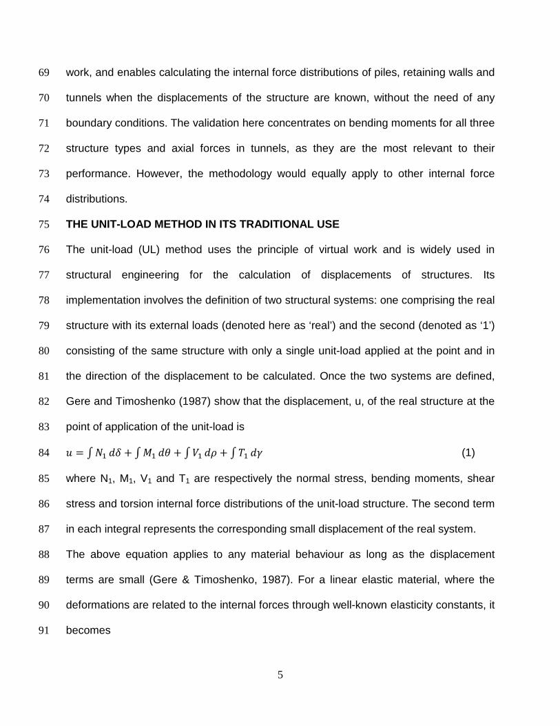
In order to apply (5) and (6), the real structures were idealised: propped walls as a 146
simply supported beam (Fig. 1a) and cantilever walls and laterally loaded piles as a 147
cantilever beam (Fig. 1b). Although these assumptions have been made by others – 148
e.g. Nig & Ng (2005) for laterally loaded piles – they are proposed and their validation is 149
part of this paper for more general conditions and geometries. 150
9
151
Figure 1. Piles and embedded retaining walls (a) UL for propped walls (b) UL for propped 152
walls for cantilever walls and laterally loaded piles (c) Displacement definitions (d) 153
Bending displacements 154
Structural observed displacements (herein called uO - See Figure 1c) can be divided into 155
three different main components (Gaba et al, 2003): rigid body rotation (ψ); rigid body 156
translation (d) and; bending (uD) as illustrated in Figure 1d. Out of the three, only the 157
latter contributes to the bending moments in the structure; hence, its isolation is needed 158
for the application of the method and should be the only component to be used. In linear 159
elastic behaviour, these can be superimposed which simplifies the process of sorting. 160
161

10
Formulation 162
Using polynomials of order n in equation (3) such as 163
)-*+ 1, )*+ , … , )0*+ 0 (7) 164
and the unit-load bending moment distributions for propped walls 165
*<+*+ S TQUGT , V W<X UGT W< , Y W< Z (8) 166
and, similarly, for cantilever walls and laterally loaded piles (see Figure 1 for variable 167
definitions), 168
*<+*+ [W< X , V W<0, Y W< Z (9) 169
the integrals in Eq. (5) and (6) become 170
M<,N TQUGT UD]FNO. W< ^X TD]NO. TD]NO UGD]F*NO.+T X UGD]NO _ (10) 171
for propped retaining walls and 172
M<,N W< UGD]NO X UGD]FNO. (11) 173
for cantilever walls and laterally loaded piles. 174
Equations (10) and (11) define the system of equations in (5) and (6) to be solved. 175
Choice of function f(x) 176
Multiple authors have chosen polynomials to approximate displacements and bending 177
moments of underground structures due to their versatility. However, the choice of order 178
is much less thoroughly explained in the literature and the reasons for choice are 179
normally justified by the amount of boundary conditions available, or a trial and error 180
procedure rather than a rigorous goodness-of-fit. A common mistake is to choose higher 181
order polynomials as they provide an apparent better fit to data; however, this may lead 182

11
to over-fitting and instabilities that are important, especially if the polynomials are used 183
to derive other parameters from its derivatives such as shear forces or soil reaction. de 184
Sousa (2006) proposed a sophisticated technique using polynomial splines in order to 185
solve this problem. The strategy proposed here to address the above problem is simple 186
and presented using Reese (1997) and Mohamad et al (2011) case studies (see Table 187
1 for description): 188
- First, the bending moments are calculated using multiple polynomial orders and Eq. 189
(5), (6), (10) and (11). Typical starting values of polynomial orders, based on 190
experience, are: 5th to 9th (Singly Propped walls), 6th to 10th (Multi-propped walls) and 4th 191
to 8th (Cantilever walls and laterally loaded piles). The above values of polynomial order 192
are only initial; iterations beyond those values may be necessary until the best order is 193
found as shown below. 194
- Model Evaluation –The Akaike Information Criterion (AIC) (Akaike, 1974) was used to 195
evaluate each polynomial. Later updates (Hurvich and Tsai, 1991), that correct for 196
models where the number of points is similar to the number of independent variables to 197
be estimated, were dismissed as it increases the risk of under-fitting (Bozogan, 1987). 198
The AIC approach provides a formulation that complies with the principle of parsimony, 199
by which the simplest model is selected, and eliminates the risk of over-fitting. AIC is 200
found using the following equation 201
`a, Xb ∗ LNeff= g 2*i 1+ (12) 202
where SSE is the Sum of Square of Errors defined as 203
jjk ∑ l)0 X )mn. (13) 204

12
and fn is the polynomial under evaluation, and )m is an estimator which is defined as the 205
average of all the polynomials used. 206
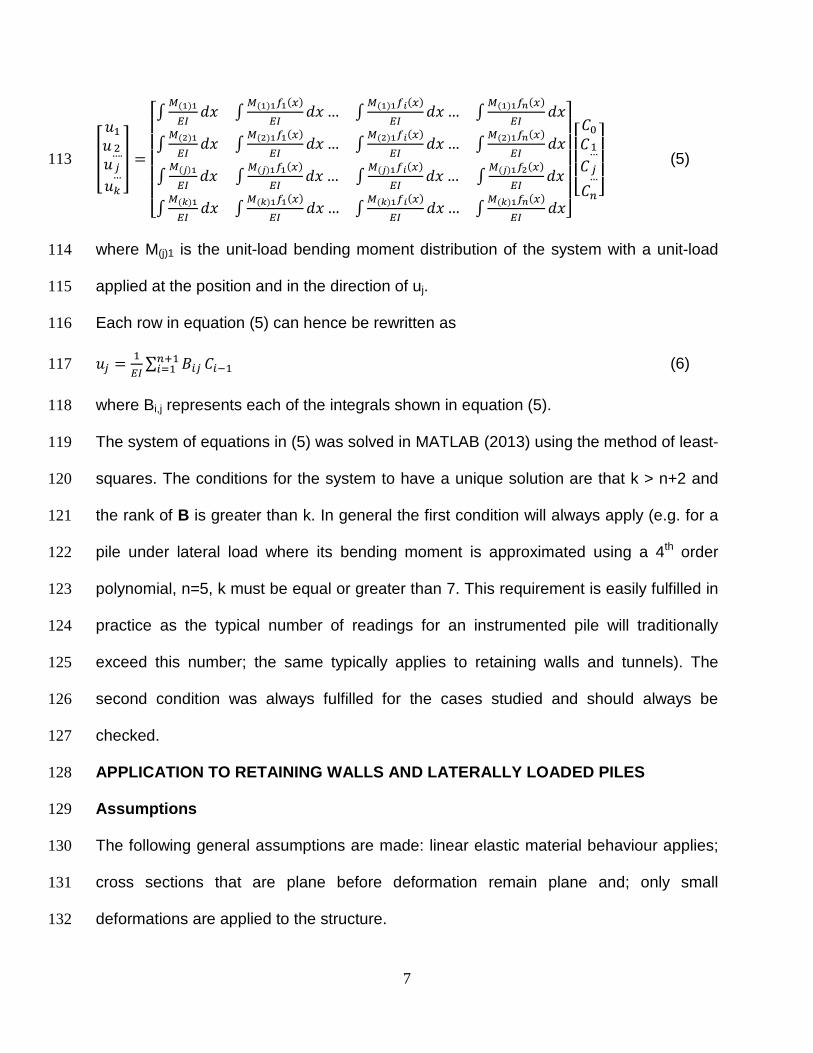
Figures 2 and 3 show the implementation of Eq. (5) and this strategy. The optimal 207
orders (lowest AIC score) are 9th for Mohamad et al (2011) and 6th for Reese (1997). 208
When the lowest AIC value corresponds to the highest or lowest polynomial order 209
considered initially, it will be necessary to reduce or increase the order until the 210
minimum is found. 211
212
213
Figure 2. Development of method for Mohamad et al (2011) (a) Polynomial choice (b) AIC 214
- Once the best order has been chosen, the final solution is taken as the average of fits 215
between the optimal polynomial order and the two closest orders with the lowest AIC 216
score. It must be noted that the two closest may be on one side of the optimal. For 217
−10 −8 −6 −4 −2 0 2 4 6x 10
−7
0
5
10
15
20
25
Curvature (1/m)
Leng
th fr
om to
e (m
)
9th
8th
7th
6thMeasuredAverage of all fits
10th & 11th
Calculated
6 7 8 9 10800
820
840
860
880
900
Polynomial order
AIC

13
example, in Mohamad et al (2011), the optimal order is 9th and 10th and 11th have lower 218
AIC scores than 8th. Hence, the final solution is taken as the average of polynomials of 219
orders 9th, 10th and 11th. 220
The above strategy was tested for all the cases in Table 1 as part of the validation 221
process below. Appendix A shows its full application, including AIC plots for all the 222
cases. 223
224
225
Figure 3. Development of method for Reese (1997) (a) Polynomial choice (b) AIC 226
Validation 227
Six case studies (described in Table 1) were analysed to validate the method’s 228
application to piles and embedded retaining walls. They portray multiple loading 229
conditions (earth pressures, tunnel induced load on piles, earthquake induced loads on 230
−1000 −500 0 500 1000 15000
1
2
3
4
5
6
7
Moment (kNm)
Leng
th fr
om to
e (m
)
8th 4th5th
6th
MeasuredAverage of all fits
7th
Calculated
4 5 6 7 8665
670
675
680
685
690
Polynomial order
AIC

14
piles, to piles embedded in sliding embankments), structural dimensions and 231
construction methodologies and hence, cover a wide spectrum of situations. 232
233
234
Figure 4. Calculation (a) Curvature (b) Input displacement - Mohamad et al (2011) 235
−10 −5 0 5x 10
−7
0
5
10
15
20
25
Curvature (1/m)
Leng
th fr
om to
e (m
)
Final
Average of all fits Observed
0 1 2 3 4 5 6 70
5
10
15
20
25
Displacement (mm)
Leng
th fr
om to
e (m
)
CalculatedReal

15
236
237
Figure 5. Calculation (a) Bending moment (b) Input displacement - Ou et al (1998) 238
−1500 −1000 −500 0 500 1000 1500 2000 25000
5
10
15
20
25
30
35
Bending moment (kNm)
Leng
th fr
om to
e (m
)
Calculated
Observed
6 7 8 9 101023
1024
1025
1026
1027
1028
1029
1030
1031
1032
1033
Polynomial order
AIC
16
239
240
Figure 6. Calculation (a) Bending moment (b) Input displacement - Reese (1997) 241
−1000 −500 0 500 1000 15000
1
2
3
4
5
6
7
Moment (kNm)
Leng
th fr
om to
e (m
)
CalculatedObserved
4 5 6 7 8665
670
675
680
685
690
Polynomial order
AIC
17
242
243
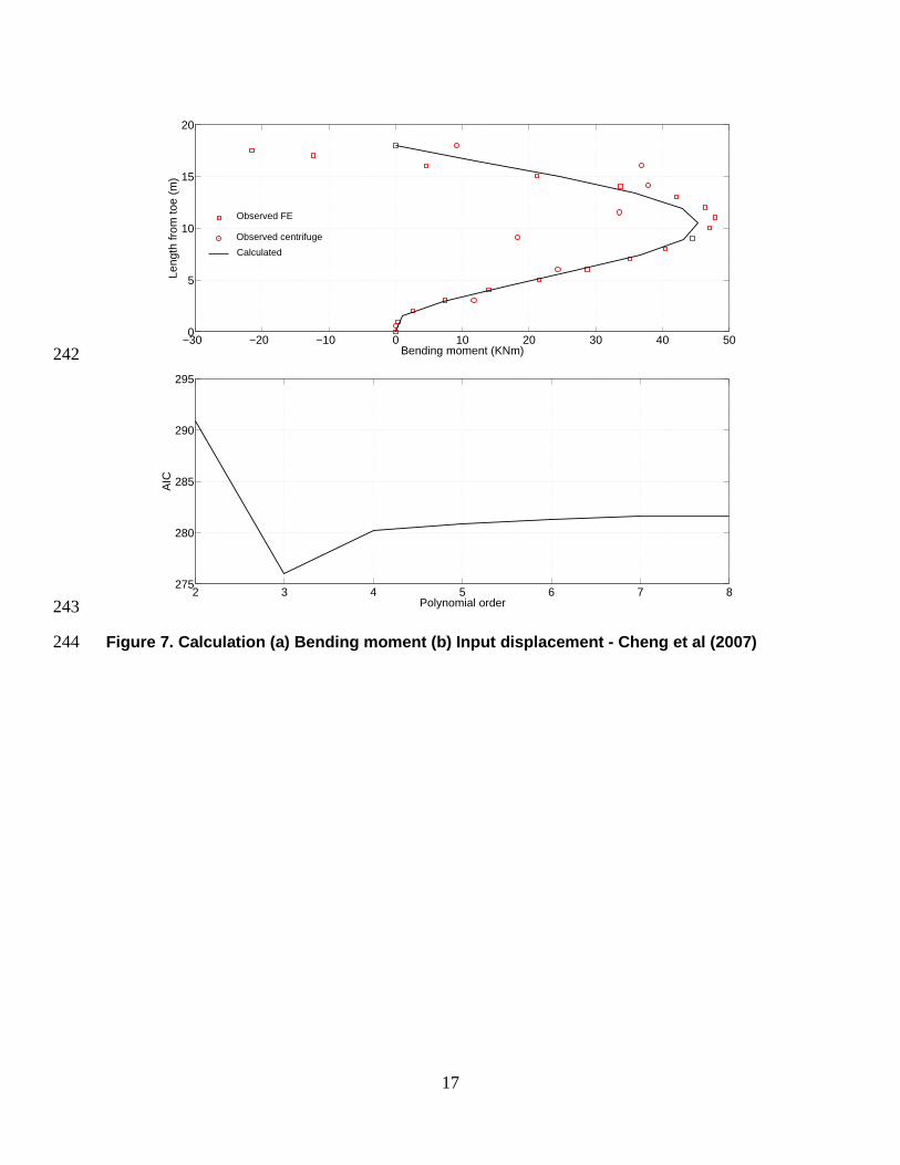
Figure 7. Calculation (a) Bending moment (b) Input displacement - Cheng et al (2007) 244
−30 −20 −10 0 10 20 30 40 500
5
10
15
20
Bending moment (KNm)
Leng
th fr
om to
e (m
)
Calculated
Observed FE
Observed centrifuge
2 3 4 5 6 7 8275
280
285
290
295
Polynomial order
AIC

18
245
246
Figure 8. Calculation (a) Bending moment (b) Input displacement - Liyanapathirana & 247
Poulos (2005) 248
249
−100 0 100 200 300 400 5000
5
10
15
20
Bending moment (kNm)
Leng
th fr
om to
e (m
)
Calculated
Observed
2 3 4 5 6 7 8305
310
315
320
325
Polynomial order
AIC

19
250
251
Figure 9. Calculation (a) Bending moment (b) Input displacement - Smethurst & Powrie 252
(2007) 253
Figures 4 to 9 show comparisons between the Calculated values (resulting from the 254
method’s application) and the Observed values (obtained from the literature). The 255
figures also show the Input displacement and the Observed values to illustrate in which 256
cases a transformation, like that shown in Figure 1d, was needed to calculate uD. 257
The match between the maximum Observed values from the literature and the 258
Calculated is within 10% for all cases, with the exception of Smethurst & Powrie (2007), 259
which is 18%. It must be noted that in this case the value of EI that was used is only an 260
−100 −50 0 50 100 150 2000
2
4
6
8
10
Bending moment (kNm)
Leng
th fr
om to
e (m
)
Calculated
Observed rebar strain gauges
Observed embedded strain gauges
4 5 6 7 8306
308
310
312
314
316
318
320
Polynomial order
AIC

20
estimate by the authors for a stage where the pile is no longer behaving fully elastically. 261
It therefore confirms the potential of the method to predict bending moments beyond the 262
elastic range if the adequate value of EI is used. 263
The Calculated values deviate, in some instances (e.g. Ou et al, 1998) towards the 264
ends of the structure, typically, the upper part, which corresponds to where the 265
displacement readings, mostly done by inclinometers, accumulate the highest errors. 266
Therefore, this source of deviation cannot be simply attributed to the method as it is 267
more likely to be mostly due to inaccuracies in displacement measurements. 268
APPLICATION TO TUNNELS 269
Assumptions 270
The same general assumptions used for piles and retaining walls apply to tunnels. 271
Here, the focus is on circular tunnels for simplicity, although the same principles apply 272
to other section shapes. It is assumed that the tunnel lining structure is monolithic (i.e. 273
the joints are not articulated) and provides full structure continuity. 274
Furthermore, it is assumed that the ratio between the radius of the tunnel and its lining 275
thickness is greater than 7 approximately and therefore, the beam can be analysed 276
using straight beams deflection theory (Roark, 1965) - i.e. equation (2) applies. This 277
assumption also allows disregarding the effect of shear forces, as the structure can be 278
considered a thin shell. 279
Radial displacements, perpendicular to the tunnel cross section, were used (see Figure 280
10). The Observed displacements (uO) can be, as in piles and retaining walls, divided 281
into two categories: those that produce bending moments and those that do not. The 282
latter, in practice, are rigid body (uRB) displacements – i.e. a translation and / or rotation 283

21
- and uniform convergence (uC) displacements – i.e. a uniform reduction in the tunnel 284
diameter (see Figure 10). The former are displacements referred here as distortion 285
displacements (uD) – typically ovalisation; however, other potential displacements such 286
as those arising from gaps behind the lining or localised loading must also be included 287
(the example shows only ovalisation deformations for simplicity). It is important to note 288
that everything that follows applies to the rotated tunnel, which means that if a rigid 289
body rotation has occurred, it needs to be removed from the observed values in 290
advance to present it as it is shown in Figure 10. 291
292
Figure 10. Tunnel displacements definitions 293
294

22
Having made the above distinction, the general equation for the radial displacements 295
can be written as 296
o pq r s (14) 297
where uO represents the Observed radial displacements of the rotated tunnel and uRB is 298
the projection of the rigid body displacement onto the radial direction for each point (e.g. 299
if the rigid body displacement is a vertical translation as in Figure 10, the tunnel crown 300
uRB is the Observed total rigid body displacement value, whereas in the springline this 301
value is zero). The sign convention in Eq. (14) is: negative for radial displacements 302
acting inwards and positive for those acting outwards. 303
The uniform convergence and rigid body displacements do not cause a change in 304
shape (i.e. the normal to tunnel lining does not change direction), which means there is 305
no shear deformation, and no bending moment. Therefore, if the normal to the tunnel at 306
the springline remains horizontal after deformation, it follows that the distortion 307
displacement at this location must also be horizontal. It also means that the vertical 308
component of the rigid body displacement is equal to the vertical component of the 309
observed displacement. Hence, if the same horizontal component of the observed 310
displacement applies at both springlines and in opposite directions, the rigid body 311
displacement must be vertical (as is the case presented in Figure 10). This reasoning 312
applies to any tunnel as long as the lining acts as a monolithic material with no joints. 313
Uniform convergence can be obtained by inspecting the tunnel cross section 314
displacements at the crown (CR) and the springline (SL) and developing (14) for each 315
ofT X pqfT r sfT (15) 316
orp X pqrp r srp (16) 317

23
In Figure 10, the distortion deformation of the example is elliptical and therefore, Eq. 318
(15) refers to displacements in the horizontal direction and (16) in the vertical direction. 319
Using the ratio between the crown and springline distortion deformations, srp/sfT, 320
substituting this into Eq. (15) and (16), subtracting algebraically both eliminates uC , and 321
isolating sfT results in 322
sfT tuvwQtxyvw QtuzxOtxyzxlQtzx tvw| n (17) 323
and inserting (17) into (15) provides the uniform convergence 324
r fT X pqfT X tuvwQtxyvw QtuzxOtxyzxlQtzx tvw| n (18) 325
This value can then be used in Eq. (14) to calculate the final distortion displacements at 326
any point in the lining 327
s o X pq X ofT pqfT tuvwQtxyvw QtuzxOtxyzxlQtzx tvw| n (19) 328
Other methods can be used to separate sources of Observed displacements. What is 329
important is to make sure that all displacements that do not produce bending moments 330
are removed in preparation for the method’s application. However, the methodology 331
presented here is deemed applicable to most cases of standard displacements in 332
tunnels and has been validated. 333
The idealisation needed for the application of the method to tunnels is shown in Figure 334
11. It consists of a thin ring with a double unit-load applied in diametrically opposite 335
locations. 336

24
337
Figure 11. Tunnel nomenclature definition and idealisation and unit-load structure 338
Formulation 339
The chosen function to represent the real structure bending moments and axial forces is 340
shown below 341
)-*+ 1, )*+ cos*+ , ).*+ cos*2+ (20) 342
which is much simpler than for piles and retaining walls as it contains only three 343
constants C (see Eq. 6) to calculate. 344
The distribution of bending moments for a generic unit-load system applied at an angle 345
bj was calculated generically for any angle f, using the equations developed by 346
Lundquist and Burke (1936) 347

25
*<+*+ *<+ *1 X sin*++*<+ sin*+*<+ , V < sinl X <n *<+ *1 X sin*++*<+ sin*+*<+ , Y < Z (21) 348
where f varies between 0 and 180o, and 349
*<+ ^*G+F O._Q (22) 350
*<+ .Q^*G+F O._ (23) 351
*<+ *G+. (24) 352
Using Eq. (20) to (24), similar equations to (10) and (11) can be derived for tunnels as 353
follows 354
M<,- *<+ *<+ X 2*<+ lcos*<+ 1n (25) 355
M<, *<+ sinl<n X*<+ l.Gn. X p lGnlQGn. (26) 356
M<,. .*<+ X p lcos*<+ 1nl2cos*<+ X 1n (27) 357
which allows redefining Eq. (6) 358
s< p∑ MN<0ONP ,NQ (28) 359
that represents the system equations from which the bending moments’ constants of 360
equation (20) can be calculated. 361
Equations (6) and (28) are almost identical with the exception of the addition of R in the 362
latter, which comes from the integration using polar coordinates and the angle f. 363
The same process applies to the axial force. In this case, the axial force caused by the 364
unit-load is 365
*<+*+ SX . sin*< X +, V <X . sin* X <+, Y < Z (29) 366
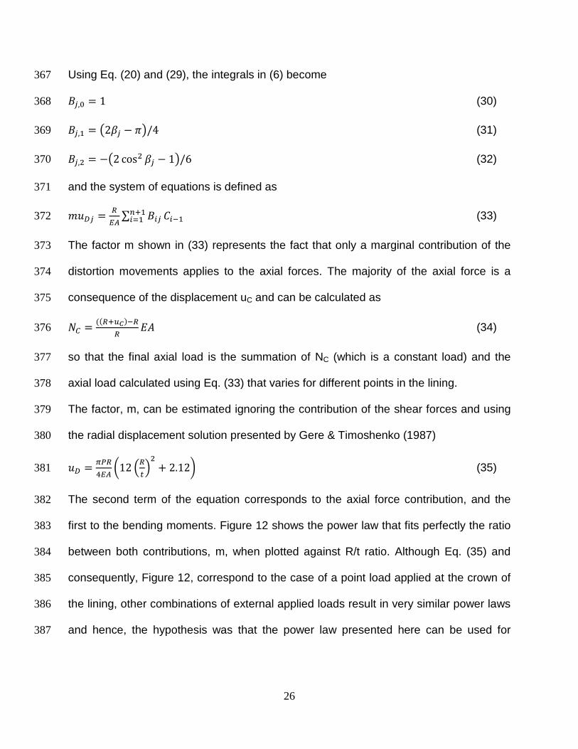
26
Using Eq. (20) and (29), the integrals in (6) become 367
M<,- 1 (30) 368
M<, l2< X n/4 (31) 369
M<,. Xl2 cos. < X 1n/6 (32) 370
and the system of equations is defined as 371
s< p∑ MN<0ONP ,NQ (33) 372
The factor m shown in (33) represents the fact that only a marginal contribution of the 373
distortion movements applies to the axial forces. The majority of the axial force is a 374
consequence of the displacement uC and can be calculated as 375
r **pOtz+Qpp k` (34) 376
so that the final axial load is the summation of NC (which is a constant load) and the 377
axial load calculated using Eq. (33) that varies for different points in the lining. 378
The factor, m, can be estimated ignoring the contribution of the shear forces and using 379
the radial displacement solution presented by Gere & Timoshenko (1987) 380
s p ^12 epg. 2.12_ (35) 381
The second term of the equation corresponds to the axial force contribution, and the 382
first to the bending moments. Figure 12 shows the power law that fits perfectly the ratio 383
between both contributions, m, when plotted against R/t ratio. Although Eq. (35) and 384
consequently, Figure 12, correspond to the case of a point load applied at the crown of 385
the lining, other combinations of external applied loads result in very similar power laws 386
and hence, the hypothesis was that the power law presented here can be used for 387

27
estimation purposes where the deformation of the tunnel is mainly elliptical. This 388
hypothesis is validated below for both case studies. 389
390
Figure 12. Ratio between axial force and bending moment contributions to radial 391
displacements 392
Choice of function f(x) 393
Most of the widely accepted solutions for tunnel lining design define the shape of 394
bending moments and radial displacements in tunnels using multiples of the cosine – 395
e.g. cos(2f) (Einstein & Schwartz, 1979; El Naggar et al, 2008; Carranza-Torres, 2013) 396
for simpler modes of deformation and cos(pf) for different orders, where p is an integer 397
greater than 1 (Muir Wood,1975). 398
Gere & Timoshenko (1987) showed that the equation linking radial displacement and 399
bending moment of a circular beam of thin section is 400
y = 0.1767x-2
R² = 1
0
0.001
0.002
0.003
0.004
0.005
0.006
0.007
0.008
0 10 20 30 40 50
m
R/t
Range of cases applicable to this paper (R/t > 10

28
Ft ¡F s X pF*¡+ (36) 401
which means that it is mathematically proven that if a function shape of the form shown 402
in (20) could be successfully fitted to the displacement profile uD, the same form would 403
apply to the bending moments, provided that EI remains constant (as it does for the 404
linear elastic region under consideration). 405
406
407
Figure 13. Validation of function choice (a) Gonzalez & Sagaseta (2001) (b) Carranza-408
Torres et al (2013). 409
Figure 13 shows the fitted proposed function in Eq. (20) to the displacement profiles 410
suggested by Gonzalez & Sagaseta (2001) and Carranza-Torres et al (2013) using the 411
MATLAB (2013) curve fitting tool. The former presents a profile where symmetry occurs 412
0 0.5 1 1.5 2 2.5 3
2
3
4
5
6
7
8
x 10−3
Angle (radians)
Rad
ial d
ispl
acem
ent (
m)
Linear model: f(x) = a + b*cos(x) + c*cos(2*x)Coefficients (with 95% confidence bounds): a = 0.004239 (0.004152, 0.004326) b = 0.00304 (0.002921, 0.003159) c = 0.0008143 (0.0006946, 0.0009339)
Goodness of fit: SSE: 5.072e−07 R−square: 0.9949 Adjusted R−square: 0.9943 RMSE: 0.000178
0 0.25 0.5 0.75 1 1.25 1.5 1.57
−0.015
−0.01
−0.005
0
0.005
0.01
0.015
Angle (radians)
Rad
ial d
ispl
acem
ent (
mm
)
Linear model: f(x) = a + b*cos(x) + c*cos (2*x)Coefficients (with 95% confidence bounds): a = −0.0009717 (−0.001836, −0.0001076) b = 0.0003633 (−0.001003, 0.00173) c = 0.01539 (0.01478, 0.016)
Goodness of fit: SSE: 5.788e−07 R−square: 0.9997 Adjusted R−square: 0.9997 RMSE: 0.0002033

29
around the vertical axis (note the x axis extends to 180o), whereas in the latter, double 413
symmetry occurs at 90o and subsequently at 180o. 414
Besides the discussion on the appropriateness of one method or another, which is 415
beyond the scope of this paper, the figure shows that the chosen function performs well 416
for both cases and provides very high values of R2 and low of RMSE, indicating an 417
acceptable goodness-of-fit. This, in turn, shows that the function is also appropriate to 418
characterise bending moments: a similar rationale applies to axial forces. 419
Validation 420
The validation was carried out against an analytical method such as Carranza-Torres et 421
al (2013) and an FE model in Brinkgreve et al (2011). The former is a more generalised 422
and complex case than those presented previously by others (e.g. Einstein & Schwartz, 423
1976) and includes complex processes such as stress relaxation. The second case is 424
representative of an accurate and calibrated FE model and programme widely used. 425
Details on both of these are presented in Table 1. 426
In order to separate the displacements, first an estimate of srp/sfT is needed. In cases 427
where the rigid body translation is small compared to the maximum distortion 428
deformations (as is the case in most tunnels), it can be estimated as orp/ofT. Hence, 429
srp/sfT values of -1.027 and -1.099 were estimated for Brinkgreve et al (2011) and 430
Carranza-Torres et al (2013) respectively. This estimate was tested through a sensitivity 431
analysis of its impact on the calculation of bending moments using the value of pure 432
shear, -0.5, and extreme values ranging between -0.92 to -1.08 (calculated from Roark 433
(1965) for the case of a triangular horizontal pressure applied on the sides). Differences 434
of less than 0.5% in the Calculated bending moment were obtained which confirmed the 435

30
adequacy of the estimate. Eq. (18) was then used to calculate uC, providing values of -436
1.383E-0m and -6.208E-04m for Brinkgreve and Carranza-Torres respectively. Finally, 437
Eq. (19) was used to calculate uD. 438
Using Eq. (34) and the calculated uC value, NC was obtained and was equal to -439
774.79kN/m (Brinkgreve et al, 2011) and -1552 kN/m (Carranza-Torres et al, 2013). The 440
m values, were estimated using the equation in Figure 14, and were 3.460E-03 and 441
1.767E-03 respectively. This allowed calculating the contribution of uD that corresponds 442
to the axial forces. 443
Figures 14 and 15 present the results of the method’s application and its comparison to 444
the observed values. The match to Carranza-Torres et al (2013) is outstanding as the fit 445
is within 0.5%. For Brinkgreve et al (2011), the method captures the fact that the 446
bending moment is marginally higher at the crown of the tunnel than at the invert, and 447
only over-predicts the latter by 14%. The Calculated axial force is closer to the 448
Observed values and only shows an error of less than 5% for its maximum values at 0 449
(and 180) and 90 degrees respectively. 450

31
451
452
Figure 14. Calculation of (a) Bending moment and Axial force (b) Input radial 453
displacement - Carranza-Torres (2013) 454
0 10 20 30 40 50 60 70 80 90−2000
−1750
−1500
−1250
−1000
Angle (degrees)
Axi
al fo
rce
(Mn/
m)
0 10 20 30 40 50 60 70 80 90−500
0
500
Ben
ding
mom
ent (
MN
m/m
)
Calculated − Axial forceObserved − Axial forceCalculated − Axial force (Nc)Calculated − Bending momentObserved − Bending moment
-0.02
-0.015
-0.01
-0.005
0
0.005
0.01
0.015
0.02
0 10 20 30 40 50 60 70 80 90
Rad
ial d
isp
lace
men
t (m
)
Angle (degrees)

32
455
456
Figure 15. Calculation of (a) Bending moment and Axial force (b) Input displacements - 457
Brinkgreve et al (2011) 458
Close inspection of Figures 14 and 15 also shows that NC is the arithmetic average of 459
the axial load for both cases and the deviation from this average is the axial load that 460
arises from the displacements muD. This deviation is also indicative of the ratio between 461
the vertical and horizontal stresses acting on the tunnel lining, as Carranza-Torres and 462
0 20 40 60 80 100 120 140 160 180−1000
−900
−800
−700
−600
Angle (degrees)
Axi
al fo
rce
(Mn/
m)
0 20 40 60 80 100 120 140 160 180−100
−50
0
50
100
Ben
ding
mom
ent (
MN
m/m
)
Observed − Axial forceCalculated − Axial forceCalculated − Axial force (Nc)Observed − Bending momentCalculated − Bending moment
-0.002
-0.0015
-0.001
-0.0005
0
0.0005
0.001
0.0015
0 30 60 90 120 150 180
Rai
dal
dis
pla
cem
ent
(m)
Angle (degrees)
Rigid bodyDistortionMeasuredUniform convergence

33
Diederichs (2009) showed, which may present future opportunities for the estimation of 463
this ratio. 464
The outstanding performance of the method against very different case studies not only 465
validates it but also the procedure presented for the separation and reasoning of the 466
different displacements contributions. 467
CONCLUSIONS 468
The proposed method is analytically correct and based on the principle of virtual work. It 469
provides a means to calculating internal forces such as bending moments and axial 470
forces without the need for boundary conditions. It solves therefore a long standing 471
problem in underground structures that has significant applications in research and 472
practice as it provides an accurate and independent check on the internal forces in a 473
structure. This is envisaged to allow producing more optimised design though greater 474
understanding of the bending moments and axial forces in underground structures. 475
The versatility and flexibility of the method has been demonstrated using diverse case 476
studies which shows it is equally applicable to piles, retaining walls and tunnels under 477
multiple loading conditions. The maximum error between Observed and Calculated 478
values of bending moment was lower than 10%, with the exception of the case where 479
slight plastic behaviour occurred and the error was 18%. 480
The method presents multiple opportunities for future work and its relevance extends 481
beyond underground structures as the same methodology is theoretically applicable to 482
any structure. Therefore, its applicability and potential usage is wide. 483
484
485

34
ACKNOWLEDGMENTS 486
The author would like to acknowledge the discussions he had and recommendations 487
received from Eden Almog (Arup Tunnelling, London) throughout the derivation of the 488
method from its original idea. It is also acknowledged the suggestions that Loretta von 489
der Tann (University College London and Arup Geotechnics) made on the part dealing 490
with piles and retaining walls and the general presentation of the paper. 491
APPENDIX A 492
This appendix shows the full application of the method to all the case studies presented 493
for piles and retaining walls. 494
495
496
−1500 −1000 −500 0 500 1000 1500 2000 25000
5
10
15
20
25
30
35
Bending moment (kNm)
Leng
th fr
om to
e (m
)
10th9th 8th
6th
7th
Average of all fits
Calculated
Observed centrifuge
6 7 8 9 101023
1024
1025
1026
1027
1028
1029
1030
1031
1032
1033
Polynomial order
AIC
35
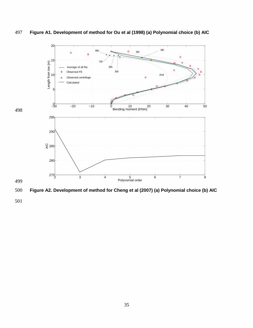
Figure A1. Development of method for Ou et al (1998) (a) Polynomial choice (b) AIC 497
498
499
Figure A2. Development of method for Cheng et al (2007) (a) Polynomial choice (b) AIC 500
501
−30 −20 −10 0 10 20 30 40 500
5
10
15
20
Bending moment (KNm)
Leng
th fr
om to
e (m
)
2nd
3th8th
7th
6th
5th
4th
Average of all fits
Calculated
Observed FE
Observed centrifuge
2 3 4 5 6 7 8275
280
285
290
295
Polynomial order
AIC

36
502
503
Figure A3. Development of method for Liyanapath. & Poulos (2005) (a) Polynomial choice 504
(b) AIC 505
−100 0 100 200 300 400 500 6000
5
10
15
20
Bending moment (kNm)
Leng
th fr
om to
e (m
)
Average of all fits
Calculated
2th
8th
3th
6th
7th
5th
4thObserved
2 3 4 5 6 7 8305
310
315
320
325
Polynomial order
AIC
37
506
507
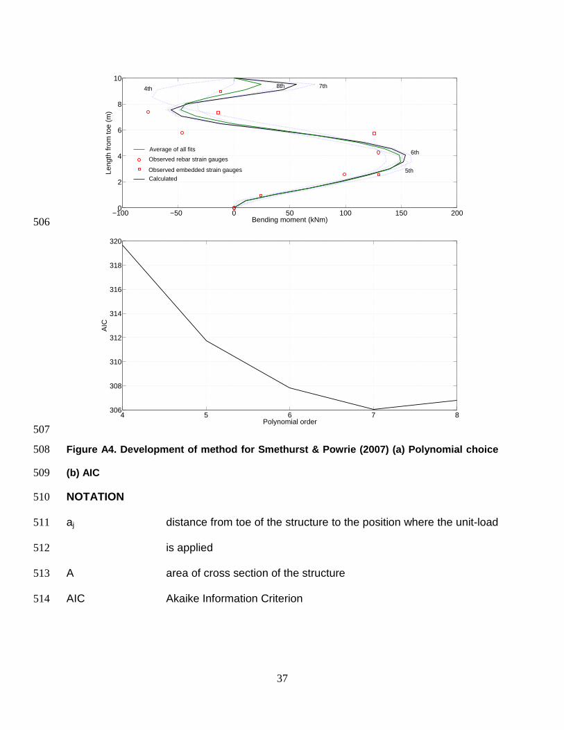
Figure A4. Development of method for Smethurst & Powrie (2007) (a) Polynomial choice 508
(b) AIC 509
NOTATION 510
aj distance from toe of the structure to the position where the unit-load 511
is applied 512
A area of cross section of the structure 513
AIC Akaike Information Criterion 514
−100 −50 0 50 100 150 2000
2
4
6
8
10
Bending moment (kNm)
Leng
th fr
om to
e (m
)
4th 7th8th
5th
Average of all fits 6th
Calculated
Observed rebar strain gauges
Observed embedded strain gauges
4 5 6 7 8306
308
310
312
314
316
318
320
Polynomial order
AIC

38
BN, BM, BV, BT matrices which elements are the integrals resulting from the 515
application of the method corresponding to the normal, moment, 516
shear and torsion internal force distributions respectively 517
C0, C1, Cj,Cn coefficients of linear equation representing the internal force 518
distribution of the real structure 519
CN, CM, CV, CT arrays of coefficients defining the normal, moment, shear and 520
torsion internal force distributions respectively 521
dδ, dθ, dρ, dγ small displacement of the real structure 522
E Young’s modulus 523
G shear modulus 524
I second moment of inertia of cross section 525
Ip polar moment of inertia 526
f0(x), f1(x),fj(x),fn(x) functions of linear equation representing the internal force 527
distribution of the real structure 528
)0 function under evaluation 529
)m estimate of function 530
h embedded length in retaining walls 531
H retained height in retaining walls 532
k number of field measurements of displacements for the real 533
structure 534
L structure length in retaining walls / piles 535
n indication on the number of functions used to approximate the 536
internal force distributions 537
39
*+ bending moment of the tunnel 538
*<+*+ bending moment in the pile / retaining wall caused by the unit-load 539
force 540
*<+*+ bending moment in the tunnel lining caused by the unit-load force 541
N1, M1, V1 and T1 normal stress, bending moments, shear stress and torsion internal 542
force distributions of the unit-load structure 543
Nreal, Mreal, Vreal 544
and Treal normal stress, bending moments, shear stress and torsion internal 545
force distributions of the real structure 546
q(x) external pressure acting on retaining walls / piles 547
q(f) external pressure acting on tunnel lining 548
R radius of tunnel 549
SSE Sum of Square of Errors 550
t tunnel lining thickness 551
x distance from the toe of the retaining wall / pile 552
u displacement of real structure in retaining walls / piles 553
u array of field Observed displacements in retaining walls / piles 554
uj displacement of the real structure at the point j where the unit-load 555
is applied 556
uD bending component of field measurement displacements in 557
retaining walls / piles 558
40
s lateral displacement of pile / retaining wall causing bending 559
moments or radial component of distortion displacement at a point 560
of the tunnel lining 561
r uniform convergence displacement 562
o observed lateral displacement of pile / retaining wall, radial 563
displacement of the tunnel lining in the rotated tunnel 564
ofT radial displacement at the tunnel springline observed 565
pq radial component of rigid body displacement at a point of the tunnel 566
lining 567
pqfT radial component of rigid body displacement at the tunnel springline 568
sfT radial component of distortion displacement at the tunnel springline 569
orp radial displacement at the tunnel crown observed 570
pqrp radial component of rigid body displacement at the tunnel crown 571
srp radial component of rigid body displacement at the tunnel crown 572
ureal field Observed displacements in retaining walls / piles 573
as shear coefficient 574
bj angle measured from the vertical direction clockwise to the point of 575
application of the unit-load 576
d translation displacement 577
f angle measured from the vertical direction at the tunnel crown and 578
clockwise 579
ψ rigid body rotation 580
REFERENCES 581
41
Abdoun, T., Dobry, R., O'Rourke, T.D., Goh, S.H. Pile response to lateral spreads: 582
Centrifuge modelling (2003). Journal of Geotechnical and Geoenvironmental 583
Engineering, 129 (10), 869-878. 584
Anagnostopoulos, C. and Georgiadis, M. (1993). Interaction of Axial and Lateral Pile 585
Responses. J. Geotechnical Engineering, 119 (4), 793–798. 586
Akaike, H. (1974). A new look at the statistical model identification. IEEE Transactions 587
on Automatic Control, 19 (6), 716–723. 588
Brown, D. A., Hidden, S. A., and Zhang, S. (1994). Determination of p-y curves using 589
inclinometer data. Geotechnical Testing Journal, 17(2), 150-158. 590
Brinkgreve, R. B. J., Swolfs, W. M. and Engin, E (2011). Plaxis Introductory: Student 591
Pack and Tutorial Manual 2010. CRC Press, Inc. Boca Raton, FL, USA. 592
Bozogan, H. (1987). Model selection and Akaike’s information criterion (AIC): The 593
general theory and its analytical extensions. Psychometrika, 52 (3), 345-370. 594
Carranza-Torres, C., Rysdahl, B., Kasim, M. On the elastic analysis of a circular lined 595
tunnel considering the delayed installation of the support (2013). International Journal of 596
Rock Mechanics and Mining Sciences, 61, 57-85. 597
Carranza-Torres, C.,and Diederichs, M. (2009). Mechanical analysis of circular liners 598
with particular reference to composite supports. For example, liners consisting of 599
shotcrete and steel sets. Tunnelling and Underground Space Technology, 24, 506–532. 600
Cheng, C.Y., Dasari, G.R., Chow, Y.K., Leung, C.F. Finite element analysis of tunnel-601
soil-pile interaction using displacement controlled model (2007). Tunnelling and 602
Underground Space Technology, 22 (4), 450-466. 603
42
Curtis,D. J. (1976). Discussion on Muir Wood. The circular tunnel in elastic ground. 604
Geotechnique, 26 (1), 213-237. 605
de Sousa Coutinho, A. (2006). Data Reduction of Horizontal Load Full-Scale Tests on 606
Bored Concrete Piles and Pile Groups. Journal of Geotechnical and Geoenvironmental 607
Engineering, 132 (6), 752-769. 608
Duddeck, H., and Erdmann, J. (1985). On structural design models for tunnels in soft 609
soil. Tunnelling and Underground Space, 9 (5-6), 246-259. 610
El Naggar, H., Hinchberger, S. D. and Lo, K.Y. (2008). A closed-form solution for 611
composite tunnel linings in a homogeneours infinite isotropic elastic medium. Canadian 612
Geotechnical Journal, 45, 266-287. 613
Fuentes, R. Study of basement design, monitoring and back-analysis to lead to 614
improved design methods. EngD Thesis, University of London, England, 2012. 615
Gaba, A., Simpson, B., Powrie, W., and Beadman D. (2003). Embedded retaining walls: 616
guidance for economic design. Report no 580. CIRIA. London. 617
Gere, J., M. and Timoshenko, S., P. (1987). Mechanics of materials, 2nd SI edition. Van 618
Nostrand Reinhold (UK) Co. Ltd, UK. 619
Gonzalez, C. and Sagaseta, C. (2001). Patterns of soil deformations around tunnels. 620
Application to the extension of Madrid Metro. Computers and Geotechnics, 28, 445–621
468. 622
Hurvich, C. M. and Tsai, C-L. (1991). Bias of the corrected AIC criterion for underfitted 623
regression and time series models, Biometrika, 78 (3), 499-509. 624

43
Inaudi, D., Vurpillot, S., Casanova, N. and Kronenberg, P. (1998). Structural monitoring 625
by curvature analysis using interferometric fibre optic sensors. Smart Materials and 626
Structures, 7, 199-208. 627
International Tunnelling Association - ITA (1998). Working group on general approaches 628
to the design of tunnels: Guideliens for the design of tunnels. Tunnelling and 629
Underground Space Technology, 3, 237-149. 630
Kim, S. H. Model testing and analysis of interactions between tunnels in clays. PhD 631
thesis, University of Oxford, England, 1996. 632
Liyanapathirana, D. S., Poulos, H. G. (2005). Seismic Lateral Response of Piles in 633
Liquefying Soil. Journal of Geotechnical and Geoenvironmental Engineering, 131 (12), 634
1466–1479. 635
Lundquist, E., E., Burke, W., F. (1936). General equations for the stress analysis of 636
rings. Report NACA-TR-509. National Advisory Committee for Aeronautics. 637
http://naca.central.cranfield.ac.uk/reports/1936/naca-report-509.pdf (Accessed on 638
11/07/2014) 639
MATLAB R2013b (8.2.0.701). Natick, Massachusetts: The MathWorks Inc., 2013. 640
Mohamad, H., Bennett, P.J., Soga, K., Mair, R.J., Bowers, K. (2010). Behaviour of an 641
old masonry tunnel due to tunnelling-induced ground settlement. Geotechnique, 60 (12), 642
927-938. 643
Mohamad, H., Soga, K., Pellew, A., Bennett, P.J. Performance monitoring of a secant-644
piled wall using distributed fiber optic strain sensing (2011). Journal of Geotechnical and 645
Geoenvironmental Engineering, 137 (12), 1236-1243. 646

44
Mohamad, H., Soga, K., Bennett, P.J., Mair, R.J., Lim, C.S. (2012). Monitoring twin 647
tunnel interaction using distributed optical fiber strain measurements. Journal of 648
Geotechnical and Geoenvironmental Engineering, 138 (8), 957-967. 649
Muir Wood, A. M. (1975). The circular tunnel in elastic ground. Geotechnique, 25(1), 650
115-127. 651
Nip, D. C. N., Ng. C. W. (2005). Back analysis of laterally loaded piles. The Institution of 652
Civil Engineers: Geotechnical Engineering, 158 (GE2), 63–73. 653
Oreste, P. P. (2003). Analysis of structural interaction in tunnels using the convergence- 654
confinement approach. Tunnelling and Underground Space Technology, 18, 347–363 655
Ou, C.-Y., Liao, J.-T., Lin, H.-D. Performance of diaphragm wall constructed using top-656
down method (1998). Journal of Geotechnical and Geoenvironmental Engineering, 124 657
(9), 798-808. 658
Panet, M. and Guenot, A. (1982). Analysis of convergence behind the face of a tunnel. 659
Proceedings Tunnelling 1982 Conference, 197-204. London 660
Reese, L. C. (1997). Analysis of laterally loaded piles in weak rock. Journal of 661
Geotechnical and Geoenvironmental Engineering, 123 (11), 1010-1017. 662
Roark, R. (1965). Formulas for stress and strain, 4th edition. Mc-Graw-Hill Kogakusha. 663
You, X., Zhang, Z., and Li, Y. (2007). An analytical method of shield tunnel based on 664
force method. Proceedings of the 33rd ITA-AITES World Tunnel Congress - 665
Underground Space - The 4th Dimension of Metropolises, 791-797. 666

Graphical Abstract (for review)