intermittency - chaosbook.orgchaosbook.org/chapters/inter.pdf · n the theory of chaotic dynamics...

Chapter 29

Intermittency

Sometimes They Come Back—Stephen King

(R. Artuso, P. Dahlqvist, G. Tanner and P. Cvitanovic)

In the theory of chaotic dynamics developed so far we assumed that the evolu-tion operators have discrete spectra {z0, z1, z2, . . . } given by the zeros of

1/ζ(z) = (· · · )∏

k

(1 − z/zk) .

The assumption was based on the tacit premise that the dynamics is everywhereexponentially unstable. Real life is nothing like that - state spaces are generi-cally infinitely interwoven patterns of stable and unstable behaviors. The stable(in the case of Hamiltonian flows, integrable) orbits do not communicate withthe ergodic components of the phase space, and can be treated by classical meth-ods. In general, one is able to treat the dynamics near stable orbits as well aschaotic components of the phase space dynamics well within a periodic orbit ap-proach. Problems occur at the borderline between chaos and regular dynamicswhere marginally stable orbits and manifolds present difficulties and still unre-solved challenges.

We shall use the simplest example of such behavior - intermittency in 1-dimensional maps - to illustrate effects of marginal stability. The main messagewill be that spectra of evolution operators are no longer discrete, dynamical zetafunctions exhibit branch cuts of the form

1/ζ(z) = (· · · ) + (1 − z)α(· · · ) ,

and correlations decay no longer exponentially, but as power laws.

546

CHAPTER 29. INTERMITTENCY 547

Figure 29.1: Typical phase space for an area-preserving map with mixed phase space dynamics;here the standard map for k = 1.2 .

29.1 Intermittency everywhere

In many fluid dynamics experiments one observes transitions from regular behav-iors to behaviors where long time intervals of regular behavior (“laminar phases”)are interrupted by fast irregular bursts. The closer the parameter is to the onset ofsuch bursts, the longer are the intervals of regular behavior. The distributions oflaminar phase intervals are well described by power laws.

This phenomenon is called intermittency, and it is a very general aspect ofdynamics, a shadow cast by non-hyperbolic, marginally stable state space regions.Complete hyperbolicity assumed in (21.5) is the exception rather than the rule,and for almost any dynamical system of interest (dynamics in smooth potentials,billiards with smooth walls, the infinite horizon Lorentz gas, etc.) one encountersmixed state spaces with islands of stability coexisting with hyperbolic regions,see figure 29.1 andexample 8.7. Wherever stable islands are interspersed withchaotic regions, trajectories which come close to the stable islands can stay ‘glued’for arbitrarily long times. These intervals of regular motion are interrupted byirregular bursts as the trajectory is re-injected into the chaotic part of the phasespace. How the trajectories are precisely ‘glued’ to the marginally stable region isoften hard to describe. What coarsely looks like a border of an island will undermagnification dissolve into infinities of island chains of decreasing sizes, brokentori and bifurcating orbits, as illustrated in figure 29.1.

Intermittency is due to the existence of fixed points and cycles of marginalstability (5.5), or (in studies of the onset of intermittency) to the proximity of anearly marginal complex or unstable orbits. In Hamiltonian systems intermittencygoes hand in hand with the existence of (marginally stable) KAM tori. In moregeneral settings, the existence of marginal or nearly marginal orbits is due to in-complete intersections of stable and unstable manifolds in a Smale horseshoe typedynamics (see figure 15.11). Following the stretching and folding of the invariantmanifolds in time one will inevitably find state space points at which the stable andunstable manifolds are almost or exactly tangential to each other, implying non-exponential separation of nearby points in state space or, in other words, marginalstability. Under small parameter perturbations such neighborhoods undergo tan-gent bifurcations - a stable/unstable pair of periodic orbits is destroyed or createdby coalescing into a marginal orbit, so the pruning which we shall encounter inchapter 15, and the intermittency discussed here are two sides of the same coin.

section 15.4

inter - 19nov2012 ChaosBook.org edition16.0, Jan 28 2018


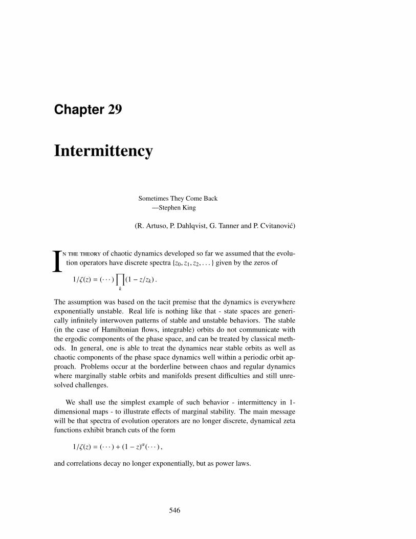
Figure 29.2: A complete binary repeller with amarginal fixed point.

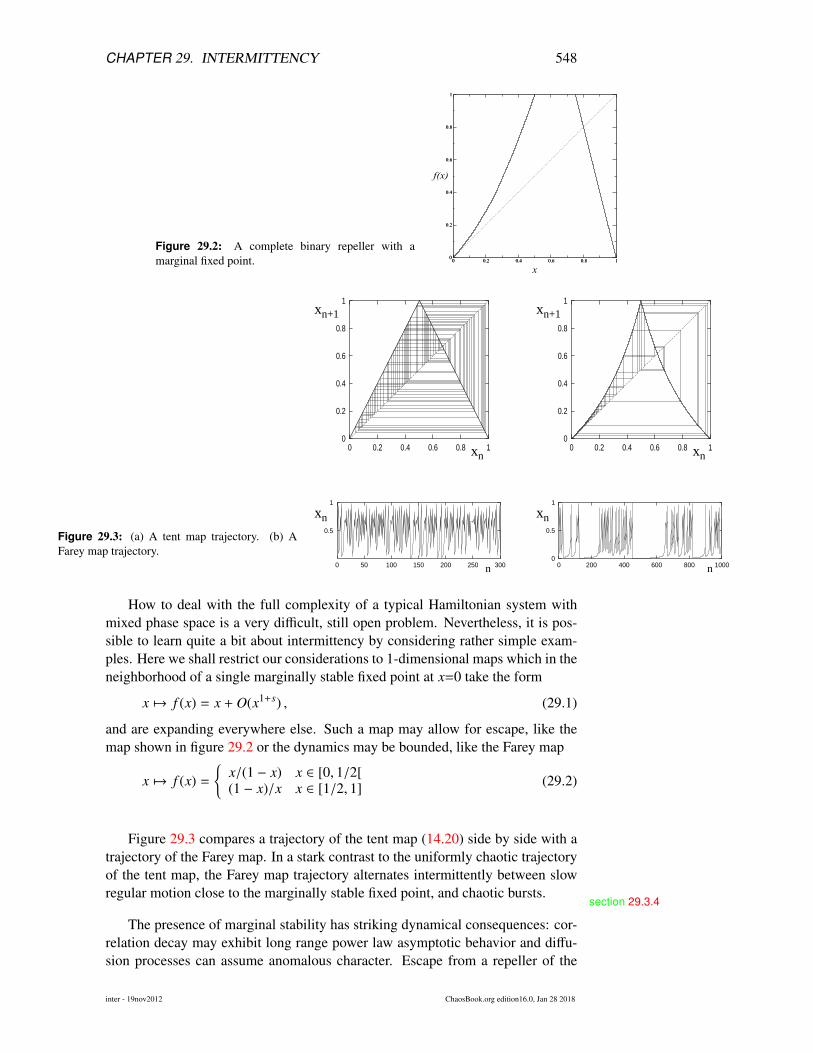
Figure 29.3: (a) A tent map trajectory. (b) AFarey map trajectory.

xn+1

xn xn

xn+1

xn xn

0

0.2

0.4

0.6

0.8

1

0 0.2 0.4 0.6 0.8 10

0.2

0.4

0.6

0.8

1

0 0.2 0.4 0.6 0.8 1

0.5

1

0 50 100 150 200 250 3000

0.5

1

0 200 400 600 800 1000n n

How to deal with the full complexity of a typical Hamiltonian system withmixed phase space is a very difficult, still open problem. Nevertheless, it is pos-sible to learn quite a bit about intermittency by considering rather simple exam-ples. Here we shall restrict our considerations to 1-dimensional maps which in theneighborhood of a single marginally stable fixed point at x=0 take the form

x 7→ f (x) = x + O(x1+s) , (29.1)

and are expanding everywhere else. Such a map may allow for escape, like themap shown in figure 29.2 or the dynamics may be bounded, like the Farey map

x 7→ f (x) =

{x/(1 − x) x ∈ [0, 1/2[(1 − x)/x x ∈ [1/2, 1] (29.2)

Figure 29.3 compares a trajectory of the tent map (14.20) side by side with atrajectory of the Farey map. In a stark contrast to the uniformly chaotic trajectoryof the tent map, the Farey map trajectory alternates intermittently between slowregular motion close to the marginally stable fixed point, and chaotic bursts.

section 29.3.4

The presence of marginal stability has striking dynamical consequences: cor-relation decay may exhibit long range power law asymptotic behavior and diffu-sion processes can assume anomalous character. Escape from a repeller of the



form figure 29.2 may be algebraic rather than exponential. In long time explo-rations of the dynamics intermittency manifests itself by enhancement of naturalmeasure in the proximity of marginally stable cycles.

The questions we shall address here are: how does marginal stability affectzeta functions or spectral determinants? And, can we deduce power law decays ofcorrelations from cycle expansions?

In example 28.5 we saw that marginal stability violates one of the conditionswhich ensure that the spectral determinant is an entire function. Already the sim-ple fact that the cycle weight 1/|1−Λr

p| in the trace (21.3) or the spectral determi-nant (22.3) diverges for marginal orbits with |Λp| = 1 tells us that we have to treatthese orbits with care.

In the following we will incorporate marginal stability orbits into cycle-expansionsin a systematic manner. To get to know the difficulties lying ahead, we will startin sect. 29.2 with a piecewise linear map, with the asymptotics (29.1). We willconstruct a dynamical zeta function in the usual way without worrying too muchabout its justification and show that it has a branch cut singularity. We will cal-culate the rate of escape from our piecewise linear map and find that it is charac-terized by decay, rather than exponential decay, a power law. We will show thatdynamical zeta functions in the presence of marginal stability can still be writtenin terms of periodic orbits, exactly as in chapters 20 and 27, with one exception:the marginally stable orbits have to be explicitly excluded. This innocent lookingstep has far reaching consequences; it forces us to change the symbolic dynamicsfrom a finite to an infinite alphabet, and entails a reorganization of the order ofsummations in cycle expansions, sect. 29.2.4.

Branch cuts are typical also for smooth intermittent maps with isolated marginallystable fixed points and cycles. In sect. 29.3, we discuss the cycle expansions andcurvature combinations for zeta functions of smooth maps tailored to intermit-tency. The knowledge of the type of singularity one encounters enables us todevelop the efficient resummation method presented in sect. 29.3.1.

Finally, in sect. 29.4, we discuss a probabilistic approach to intermittency thatyields approximate dynamical zeta functions and provides valuable informationabout more complicated systems, such as billiards.

29.2 Intermittency for pedestrians

Intermittency does not only present us with a large repertoire of interesting dy-namics, it is also at the root of many sorrows such as slow convergence of cycleexpansions. In order to get to know the kind of problems which arise when study-ing dynamical zeta functions in the presence of marginal stability we will consideran artfully concocted piecewise linear model first. From there we will move on tothe more general case of smooth intermittant maps, sect. 29.3.



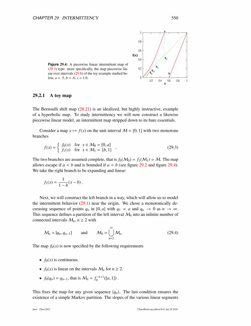
Figure 29.4: A piecewise linear intermittent map of(29.3) type: more specifically, the map piecewise lin-ear over intervals (29.8) of the toy example studied be-low, a = .5, b = .6, s = 1.0.

x

q

qq

q

f(x)

a

0

0.2

0.4

0.6

0.8

1

0.2 0.4 0.6 0.8 1

3

.

2

4

1

b..

29.2.1 A toy map

The Bernoulli shift map (28.21) is an idealized, but highly instructive, exampleof a hyperbolic map. To study intermittency we will now construct a likewisepiecewise linear model, an intermittent map stripped down to its bare essentials.

Consider a map x 7→ f (x) on the unit intervalM = [0, 1] with two monotonebranches

f (x) =

{f0(x) for x ∈ M0 = [0, a]f1(x) for x ∈ M1 = [b, 1] . (29.3)

The two branches are assumed complete, that is f0(M0) = f1(M1) =M. The mapallows escape if a < b and is bounded if a = b (see figure 29.2 and figure 29.4).We take the right branch to be expanding and linear:

f1(x) =1

1 − b(x − b) .

Next, we will construct the left branch in a way, which will allow us to modelthe intermittent behavior (29.1) near the origin. We chose a monotonically de-creasing sequence of points qn in [0, a] with q1 = a and qn → 0 as n → ∞.This sequence defines a partition of the left intervalM0 into an infinite number ofconnected intervalsMn, n ≥ 2 with

Mn = ]qn, qn−1] and M0 =

∞⋃n=2

Mn. (29.4)

The map f0(x) is now specified by the following requirements

• f0(x) is continuous.

• f0(x) is linear on the intervalsMn for n ≥ 2.

• f0(qn) = qn−1, that isMn = f −n+10 ([a, 1]) .

This fixes the map for any given sequence {qn}. The last condition ensures theexistence of a simple Markov partition. The slopes of the various linear segments



are

f ′0(x) =f0(qn−1)− f0(qn)

qn−1−qn=

|Mn−1 ||Mn |

for x ∈ Mn, n ≥ 3f ′0(x) =

f0(q1)− f0(q2)q1−q2

= 1−a|M2 |

for x ∈ M2

f ′0(x) = 11−b =

|M|

|M1 |for x ∈ M1

(29.5)

with |Mn| = qn−1 − qn for n ≥ 2. Note that we do not require as yet that the mapexhibit intermittent behavior.

We will see that the family of periodic orbits with code 10n plays a key rolefor intermittent maps of the form (29.1). An orbit 10n enters the intervalsM1 →

Mn+1 → Mn → . . . → M2 successively and the family approaches the marginalstable fixed point at x = 0 for n → ∞. The stability of a cycle 10n for n ≥ 1 isgiven by the chain rule (4.43),

Λ10n = f ′0(xn+1) f ′0(xn) . . . f ′0(x2) f ′1(x1) =1

|Mn+1|

1 − a1 − b

, (29.6)

with xi ∈ Mi.

The properties of the map (29.3) are completely determined by the sequence{qn}. By choosing qn = 2−n, for example, we recover the uniformly hyperbolicBernoulli shift map (28.21). An intermittent map of the form (29.4) having theasymptotic behavior (29.1) can be constructed by choosing an algebraically de-caying sequence {qn} behaving asymptotically like

qn ∼1

n1/s ,

where s is the intermittency exponent in (29.1). Such a partition leads to intervalswhose length decreases asymptotically like a power-law, that is,

|Mn| ∼1

n1+1/s . (29.7)

As can be seen from (29.6), the Floquet multipliers of periodic orbit families ap-proaching the marginal fixed point, such as the 10n family increase in turn onlyalgebraically with the cycle length.

It may now seem natural to construct an intermittent toy map in terms of apartition |Mn| = 1/n1+1/s, that is, a partition which follows (29.7) exactly. Sucha choice leads to a dynamical zeta function which can be written in terms of so-called Jonquière functions (or polylogarithms) which arise naturally also in thecontext of the Farey map (29.2), and the anomalous diffusion of sect. 24.3. We

remark 24.7will, however, not go along this route here; instead, we will engage in a bit ofreverse engineering and construct a less obvious partition which will simplify thealgebra considerably later without loosing any of the key features typical for inter-mittent systems. We fix the intermittent toy map by specifying the intervalsMn

in terms of Gamma functions according to

|Mn| = CΓ(n + m − 1/s − 1)

Γ(n + m)for n ≥ 2, (29.8)



where m = [1/s] denotes the integer part of 1/s and C is a normalization constantfixed by the condition

∑∞n=2 |Mn| = q1 = a, that is,

C = a

∞∑n=m+1

Γ(n − 1/s)Γ(n + 1)

−1

. (29.9)

Using Stirling’s formula for the Gamma function

Γ(z) ∼ e−zzz−1/2√

2π (1 + 1/12z + . . .) ,

we verify that the intervals decay asymptotically like n−(1+1/s), as required by thecondition (29.7).

Next, let us write down the dynamical zeta function of the toy map in termsof its periodic orbits, that is

1/ζ(z) =∏

p

(1 −

znp

|Λp|

)One may be tempted to expand the dynamical zeta function in terms of the binarysymbolic dynamics of the map; we saw, however, in sect. 23.7 that such cycle ex-pansion converges extremely slowly. The shadowing mechanism between orbitsand pseudo-orbits fails for orbits of the form 10n with stabilities given by (29.6),due to the marginal stability of the fixed point 0. It is therefore advantageous tochoose as the fundamental cycles the family of orbits with code 10n or, equiva-lently, switch from the finite (binary) alphabet to an infinite alphabet given by

10n−1 → n.

Due to the piecewise-linear form of the map which maps intervals Mn exactlyontoMn−1, all periodic orbits entering the left branch at least twice are canceledexactly by pseudo cycles, and the cycle expanded dynamical zeta function dependsonly on the fundamental series 1, 10, 100, . . .:

1/ζ(z) =∏p,0

(1 −

znp

|Λp|

)= 1 −

∞∑n=1

zn

|Λ10n−1 |

= 1 − (1 − b)z − C1 − b1 − a

∞∑n=2

Γ(n + m − 1/s − 1)Γ(n + m)

zn . (29.10)

The fundamental term (23.8) consists here of an infinite sum over algebraicallydecaying cycle weights. The sum is divergent for |z| ≥ 1. We will see that thisbehavior is due to a branch cut of 1/ζ starting at z = 1. We need to find analyticcontinuations of sums over algebraically decreasing terms in (29.10). Note alsothat we omitted the fixed point 0 in the above Euler product; we will discussedthis point as well as a proper derivation of the zeta function in more detail insect. 29.2.4.



29.2.2 Branch cuts

Starting from the dynamical zeta function (29.10), we first have to worry aboutfinding an analytical continuation of the sum for |z| ≥ 1. We do, however, get thispart for free here due to the particular choice of interval lengths made in (29.8).The sum over ratios of Gamma functions in (29.10) can be evaluated analyticallyby using the following identities valid for 1/s = α > 0 (the famed binomialtheorem in disguise),

• α non-integer

(1 − z)α =

∞∑n=0

Γ(n − α)Γ(−α)Γ(n + 1)

zn (29.11)

• α integer

(1 − z)α log(1 − z) =

α∑n=1

(−1)ncnzn (29.12)

+ (−1)α+1α!∞∑

n=α+1

(n − α − 1)!n!

zn

with

cn =

(αn

) n−1∑k=0

1α − k

.

In order to simplify the notation, we restrict the intermittency parameter to therange 1 ≤ 1/s < 2 with [1/s] = m = 1. All what follows can easily be generalizedto arbitrary s > 0 using equations (29.11) and (29.12). The infinite sum in (29.10)can now be evaluated with the help of (29.11) or (29.12), that is,

∞∑n=2

Γ(n − 1/s)Γ(n + 1)

zn =

{Γ(− 1

s )[(1 − z)1/s − 1 + 1

s z]

for 1 < 1/s < 2;(1 − z) log(1 − z) + z for s = 1 .

The normalization constant C in (29.8) can be evaluated explicitly using (29.9)and the dynamical zeta function can be given in closed form. We obtain for 1 <

1/s < 2

1/ζ(z) = 1 − (1 − b)z −a

1/s − 11 − b1 − a

((1 − z)1/s − 1 +

1s

z). (29.13)

and for s = 1,

1/ζ(z) = 1 − (1 − b)z − a1 − b1 − a

((1 − z) log(1 − z) + z

). (29.14)

It now becomes clear why the particular choice of intervalsMn made in the lastsection is useful; by summing over the infinite family of periodic orbits 0n1 ex-plicitly, we have found the desired analytical continuation for the dynamical zeta



function for |z| ≥ 1. The function has a branch cut starting at the branch point z = 1and running along the positive real axis. That means, the dynamical zeta functiontakes on different values when approaching the positive real axis for Re z > 1 fromabove and below. The dynamical zeta function for general s > 0 takes on the form

1/ζ(z) = 1 − (1 − b)z −a

gs(1)1 − b1 − a

1zm−1

((1 − z)1/s − gs(z)

)(29.15)

for non-integer s with m = [1/s] and

1/ζ(z) = 1− (1− b)z−a

gm(1)1 − b1 − a

1zm−1

((1 − z)m log(1 − z) − gm(z)

)(29.16)

for 1/s = m integer and gs(z) are polynomials of order m = [1/s] which canbe deduced from (29.11) or (29.12). We thus find algebraic branch cuts for noninteger intermittency exponents 1/s and logarithmic branch cuts for 1/s integer.We will see in sect. 29.3 that branch cuts of that form are generic for 1-dimensionalintermittent maps.

Branch cuts are the all important new feature of dynamical zeta functions dueto intermittency. So, how do we calculate averages or escape rates of the dynamicsof the map from a dynamical zeta function with branch cuts? We take ‘a learningby doing’ approach and calculate the escape from our toy map for a < b.

29.2.3 Escape rate

Our starting point for the calculation of the fraction of survivors after n time steps,is the integral representation (22.15)

Γn =1

2πi

∮γ−r

z−n(

ddz

log ζ−1(z))

dz , (29.17)

where the contour encircles the origin in the clockwise direction. If the contourlies inside the unit circle |z| = 1, we may expand the logarithmic derivative ofζ−1(z) as a convergent sum over all periodic orbits. Integrals and sums can beinterchanged, the integrals can be solved term by term, and the formula (21.22)is recovered. For hyperbolic maps, cycle expansion methods or other techniquesmay provide an analytic extension of the dynamical zeta function beyond the lead-ing zero; we may therefore deform the original contour into a larger circle with ra-dius R which encircles both poles and zeros of ζ−1(z), see figure 29.5 (a). Residuecalculus turns this into a sum over the zeros zα and poles zβ of the dynamical zetafunction, that is

Γn =

zeros∑|zα |<R

1znα−

poles∑|zβ |<R

1znβ

+1

2πi

∮γ−R

dz z−n ddz

log ζ−1, (29.18)

where the last term gives a contribution from a large circle γ−R . We thus findexponential decay of Γn dominated by the leading zero or pole of ζ−1(z).



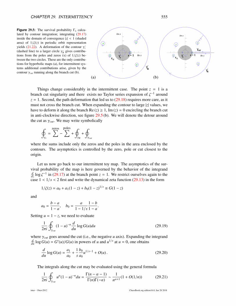
Figure 29.5: The survival probability Γn calcu-lated by contour integration; integrating (29.17)inside the domain of convergence |z| < 1 (shadedarea) of 1/ζ(z) in periodic orbit representationyields (21.22). A deformation of the contour γ−r(dashed line) to a larger circle γ−R gives contribu-tions from the poles and zeros (x) of 1/ζ(z) be-tween the two circles. These are the only contribu-tions for hyperbolic maps (a), for intermittent sys-tems additional contributions arise, given by thecontour γcut running along the branch cut (b).

(a)

Im z

-

γR-

γ z = 1zα

rRe z

(b)

Im z

- z = 1zα

γ

γR -

γcut

rRe z

Things change considerably in the intermittent case. The point z = 1 is abranch cut singularity and there exists no Taylor series expansion of ζ−1 aroundz = 1. Second, the path deformation that led us to (29.18) requires more care, as itmust not cross the branch cut. When expanding the contour to large |z| values, wehave to deform it along the branch Re (z) ≥ 1, Im (z) = 0 encircling the branch cutin anti-clockwise direction, see figure 29.5 (b). We will denote the detour aroundthe cut as γcut. We may write symbolically∮

γr

=

zeros∑−

poles∑+

∮γR

+

∮γcut

where the sums include only the zeros and the poles in the area enclosed by thecontours. The asymptotics is controlled by the zero, pole or cut closest to theorigin.

Let us now go back to our intermittent toy map. The asymptotics of the sur-vival probability of the map is here governed by the behavior of the integrandddz log ζ−1 in (29.17) at the branch point z = 1. We restrict ourselves again to thecase 1 < 1/s < 2 first and write the dynamical zeta function (29.13) in the form

1/ζ(z) = a0 + a1(1 − z) + b0(1 − z)1/s ≡ G(1 − z)

and

a0 =b − a1 − a

, b0 =a

1 − 1/s1 − b1 − a

.

Setting u = 1 − z, we need to evaluate

12πi

∮γcut

(1 − u)−n ddu

log G(u)du (29.19)

where γcut goes around the cut (i.e., the negative u axis). Expanding the integrandddu log G(u) = G′(u)/G(u) in powers of u and u1/s at u = 0, one obtains

ddu

log G(u) =a1

a0+

1s

b0

a0u1/s−1 + O(u) . (29.20)

The integrals along the cut may be evaluated using the general formula

12πi

∮γcut

uα(1 − u)−ndu =Γ(n − α − 1)Γ(n)Γ(−α)

∼1

nα+1 (1 + O(1/n)) (29.21)



Figure 29.6: The asymptotic escape from an intermit-tent repeller is a power law. Normally it is precededby an exponential, which can be related to zeros closeto the cut but beyond the branch point z = 1, as infigure 29.5 (b).

which can be obtained by deforming the contour back to a loop around the pointu = 1, now in positive (anti-clockwise) direction. The contour integral then picksup the (n−1)st term in the Taylor expansion of the function uα at u = 1, cf. (29.11).For the continuous time case the corresponding formula is

12πi

∮γcut

zαeztdz =1

Γ(−α)1

tα+1 . (29.22)

Plugging (29.20) into (29.19) and using (29.21) we get the asymptotic result

Γn ∼b0

a0

1s

1Γ(1 − 1/s)

1n1/s =

as − 1

1 − bb − a

1Γ(1 − 1/s)

1n1/s . (29.23)

We see that, asymptotically, the escape from an intermittent repeller is describedby power law decay rather than the exponential decay we are familiar with forhyperbolic maps; a numerical simulation of the power-law escape from an inter-mittent repeller is shown in figure 29.6.

For general non-integer 1/s > 0, we write

1/ζ(z) = A(u) + (u)1/sB(u) ≡ G(u)

with u = 1 − z and A(u), B(u) are functions analytic in a disc of radius 1 aroundu = 0. The leading terms in the Taylor series expansions of A(u) and B(u) are

a0 =b − a1 − a

, b0 =a

gs(1)1 − b1 − a

,

see (29.15). Expanding ddu log G(u) around u = 0, one again obtains leading or-

der contributions according to (29.20) and the general result follows immediatelyusing (29.21), that is,

Γn ∼a

sgs(1)1 − bb − a

1Γ(1 − 1/s)

1n1/s . (29.24)

Applying the same arguments for integer intermittency exponents 1/s = m, oneobtains

Γn ∼ (−1)m+1 asgm(1)

1 − bb − a

m!nm . (29.25)

So far, we have considered the survival probability for a repeller, that is weassumed a < b. The formulas (29.24) and (29.25) do obviously not apply for the



case a = b, that is, for the bounded map. The coefficient a0 = (b − a)/(1 − a)in the series representation of G(u) is zero, and the expansion of the logarithmicderivative of G(u) (29.20) is no longer valid. We get instead

ddu

log G(u) =

1u

(1 + O(u1/s−1)

)s < 1

1u

(1s + O(u1−1/s)

)s > 1

,

assuming non-integer 1/s for convenience. One obtains for the survival probabil-ity.

Γn ∼

{1 + O(n1−1/s) s < 1

1/s + O(n1/s−1) s > 1 .

For s > 1, this is what we expect. There is no escape, so the survival probabilityis equal to 1, which we get as an asymptotic result here. The result for s > 1 issomewhat more worrying. It says that Γn defined as sum over the instabilities ofthe periodic orbits as in (27.18) does not tend to unity for large n. However, thecase s > 1 is in many senses anomalous. For instance, the invariant density cannotbe normalized. It is therefore not reasonable to expect that periodic orbit theorieswill work without complications.

29.2.4 Why does it work (anyway)?

Due to the piecewise linear nature of the map constructed in the previous section,we had the nice property that interval lengths did exactly coincide with the inverseof the stability of periodic orbits of the system, that is

|Mn| = 1/|Λ10|n−1.

There is thus no problem in replacing the survival probability Γn given by (1.2),(27.2), that is the fraction of state spaceM surviving n iterations of the map,

Γn =1|M|

(n)∑i

|Mi| .

by a sum over periodic orbits of the form (21.22). The only orbit to worry about isthe marginal fixed point 0 itself which we excluded from the zeta function (29.10).

For smooth intermittent maps, things are less clear and the fact that we had toprune the marginal fixed point is a warning sign that interval estimates by periodicorbit stabilities might go horribly wrong. The derivation of the survival probabilityin terms of cycle stabilities in chapter 27 did indeed rely heavily on a hyperbolicityassumption which is clearly not fulfilled for intermittent maps. We therefore haveto carefully reconsider this derivation in order to show that periodic orbit formulasare actually valid for intermittent systems in the first place.

We will for simplicity consider maps, which have a finite number of say sbranches defined on intervals Ms and we assume that the map maps each inter-val Ms onto M, that is f (Ms) = M. This ensures the existence of a completesymbolic dynamics - just to make things easy (see figure 29.2).



The generating partition is composed of the domainsMs . The nth level parti-tion C(n) = {Mi} can be constructed iteratively. Here i’s are words i = s2s2 . . . sn

of length n, and the intervalsMi are constructed recursively

Ms j = f −1s (M j) , (29.26)

where s j is the concatenation of letter s with word j of length n j < n.

In what follows we will concentrate on the survival probability Γn , postponingother quantities of interest, such as averages, to later considerations. In establish-ing the equivalence of the survival probability and the periodic orbit formula forthe escape rate for hyperbolic systems we have assumed that the map is expand-ing, with a minimal expansion rate | f ′(x)| ≥ Λmin > 1. This enabled us to boundthe size of every survivor stripMi by (27.6), the stability Λi of the periodic orbit iwithin theMi, and bound the survival probability by the periodic orbit sum (27.7).

The bound (27.6)

C11|Λi|

<|Mi|

|M|< C2

1|Λi|

relies on hyperbolicity, and is thus indeed violated for intermittent systems. Theproblem is that now there is no lower bound on the expansion rate, the minimalexpansion rate is Λmin = 1. The survivor stripM0n which includes the marginalfixed point is thus completely overestimated by 1/|Λ0n | = 1 which is constant forall n.

exercise 22.6

However, bounding survival probability strip by strip is not what is requiredfor establishing the bound (27.7). For intermittent systems a somewhat weakerbound can be established, saying that the average size of intervals along a periodicorbit can be bounded close to the stability of the periodic orbit for all but theinterval M0n . The weaker bound applies to averaging over each prime cycle pseparately

C11|Λp|

<1np

∑i∈p

|Mi|

|M|< C2

1|Λp|

, (29.27)

where the word i represents a code of the periodic orbit p and all its cyclic permu-tations. It can be shown that one can find positive constants C1, C2 independentof p. Summing over all periodic orbits leads then again to (27.7).

To study averages of multiplicative weights we follow sect. 20.1 and introducea state space observable a(x) and the integrated quantity

A(x, n) =

n−1∑k=0

a( f k(x)).

This leads us to introduce the moment-generating function (20.9)

〈eβ A(x,n)〉,



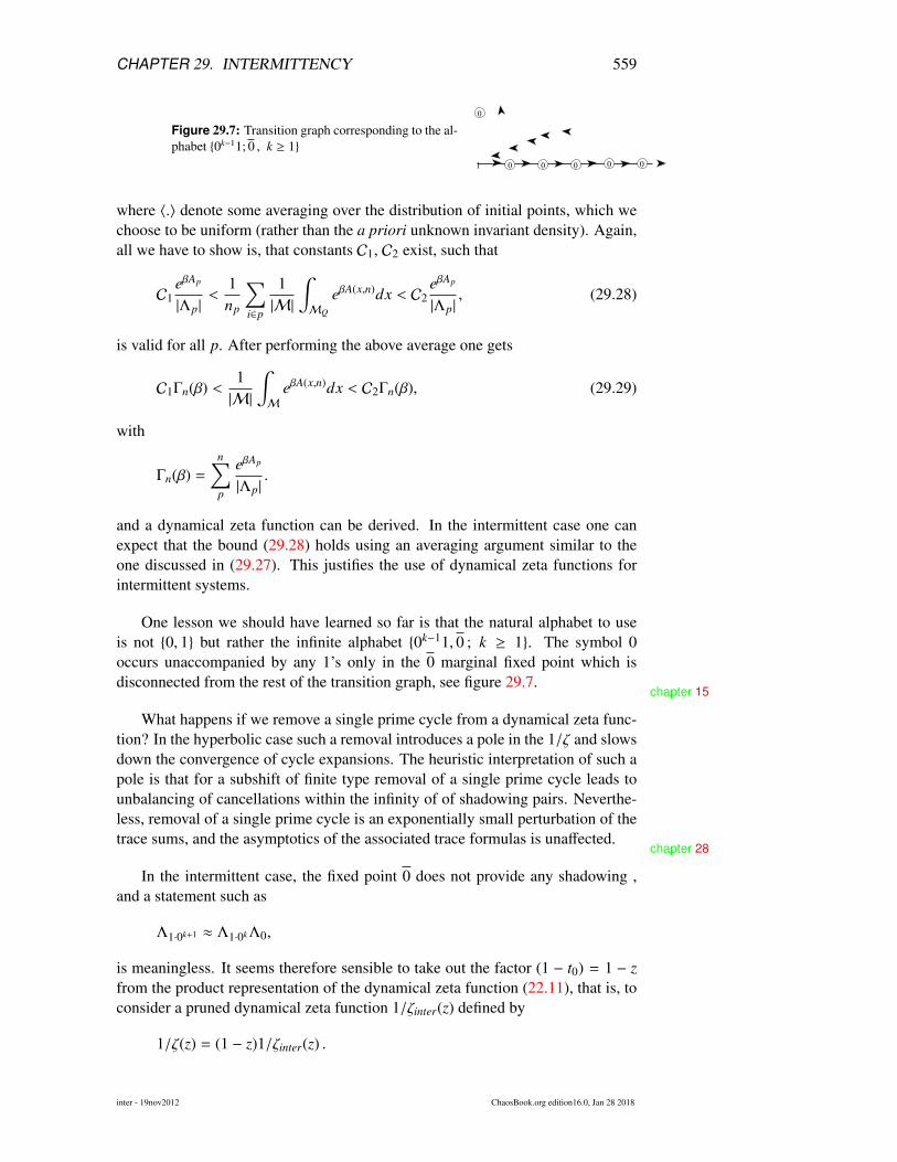
Figure 29.7: Transition graph corresponding to the al-phabet {0k−11; 0 , k ≥ 1}

where 〈.〉 denote some averaging over the distribution of initial points, which wechoose to be uniform (rather than the a priori unknown invariant density). Again,all we have to show is, that constants C1, C2 exist, such that

C1eβAp

|Λp|<

1np

∑i∈p

1|M|

∫MQ

eβA(x,n)dx < C2eβAp

|Λp|, (29.28)

is valid for all p. After performing the above average one gets

C1Γn(β) <1|M|

∫M

eβA(x,n)dx < C2Γn(β), (29.29)

with

Γn(β) =

n∑p

eβAp

|Λp|.

and a dynamical zeta function can be derived. In the intermittent case one canexpect that the bound (29.28) holds using an averaging argument similar to theone discussed in (29.27). This justifies the use of dynamical zeta functions forintermittent systems.

One lesson we should have learned so far is that the natural alphabet to useis not {0, 1} but rather the infinite alphabet {0k−11, 0 ; k ≥ 1}. The symbol 0occurs unaccompanied by any 1’s only in the 0 marginal fixed point which isdisconnected from the rest of the transition graph, see figure 29.7.

chapter 15

What happens if we remove a single prime cycle from a dynamical zeta func-tion? In the hyperbolic case such a removal introduces a pole in the 1/ζ and slowsdown the convergence of cycle expansions. The heuristic interpretation of such apole is that for a subshift of finite type removal of a single prime cycle leads tounbalancing of cancellations within the infinity of of shadowing pairs. Neverthe-less, removal of a single prime cycle is an exponentially small perturbation of thetrace sums, and the asymptotics of the associated trace formulas is unaffected.

chapter 28

In the intermittent case, the fixed point 0 does not provide any shadowing ,and a statement such as

Λ1·0k+1 ≈ Λ1·0kΛ0,

is meaningless. It seems therefore sensible to take out the factor (1 − t0) = 1 − zfrom the product representation of the dynamical zeta function (22.11), that is, toconsider a pruned dynamical zeta function 1/ζinter(z) defined by

1/ζ(z) = (1 − z)1/ζinter(z) .



We saw in the last sections, that the zeta function 1/ζinter(z) has all the nice prop-erties we know from the hyperbolic case, that is, we can find a cycle expansionwith - in the toy model case - vanishing curvature contributions and we can calcu-late dynamical properties like escape after having understood, how to handle thebranch cut. But you might still be worried about leaving out the extra factor 1 − zall together. It turns out, that this is not only a matter of convenience, omittingthe marginal 0 cycle is a dire necessity. The cycle weight Λn

0 = 1 overestimatesthe corresponding interval length ofM0n in the partition of the state spaceM byan increasing amount thus leading to wrong results when calculating escape. Byleaving out the 0 cycle (and thus also theM0n contribution), we are guaranteed toget at least the right asymptotical behavior.

Note also, that if we are working with the spectral determinant (22.3), givenin product form as

det (1 − zL) =∏

p

∞∏m=0

(1 −

znp

|Λp|Λmp

),

for intermittent maps the marginal stable cycle has to be excluded. It introducesan (unphysical) essential singularity at z = 1 due the presence of a factor (1 − z)∞

stemming from the 0 cycle.

29.3 Intermittency for cyclists

Admittedly, the toy map is what is says - a toy model. The piece wise linear-ity of the map led to exact cancellations of the curvature contributions leavingonly the fundamental terms. There are still infinitely many orbits included in thefundamental term, but the cycle weights were chosen in such a way that the zetafunction could be written in closed form. For a smooth intermittent map this allwill not be the case in general; still, we will argue that we have already seen al-most all the fundamentally new features due to intermittency. What remains aretechnicalities - not necessarily easy to handle, but nothing very surprise any more.

In the following we will sketch, how to make cycle expansion techniques workfor general 1-dimensional maps with a single isolated marginal fixed point. Tokeep the notation simple, we will consider two-branch maps with a complete bi-nary symbolic dynamics as for example the Farey map, figure 29.3, or the repellerdepicted in figure 29.2. We again assume that the behavior near the fixed point isgiven by (29.1). This implies that the stability of a family of periodic orbits ap-proaching the marginally stable orbit, as for example the family 10n, will increaseonly algebraically, that is we find again for large n

1Λ10n

∼1

n1+1/s ,

where s denotes the intermittency exponent.

When considering zeta functions or trace formulas, we again have to take outthe marginal orbit 0; periodic orbit contributions of the form t0n1 are now unbal-anced and we arrive at a cycle expansion in terms of infinitely many fundamental



Table 29.1: Infinite alphabet versus the original binary alphabet for the shortest periodicorbit families. Repetitions of prime cycles (11 = 12, 0101 = 012, . . .) and their cyclicrepeats (110 = 101, 1110 = 1101, . . .) are accounted for by cancelations and combinationfactors in the cycle expansion (29.30).

∞ – alphabet binary alphabetn = 1 n = 2 n = 3 n = 4 n = 5

1-cycles n 1 10 100 1000 100002-cycles mn

1n 11 110 1100 11000 1100002n 101 0101 10100 101000 10100003n 1001 10010 100100 1001000 100100004n 10001 100010 1000100 10001000 100010000

3-cycles kmn11n 111 1110 11100 111000 111000012n 1101 11010 110100 1101000 1101000013n 11001 110010 1100100 11001000 11001000021n 1011 10110 101100 1011000 1011000022n 10101 101010 1010100 10101000 10101000023n 101001 1010010 10100100 101001000 101001000031n 10011 100110 1001100 10011000 10011000032n 100101 1001010 10010100 100101000 100101000033n 1001001 10010010 100100100 1001001000 10010010000

terms as for our toy map. This corresponds to moving from our binary symbolicdynamics to an infinite symbolic dynamics by making the identification

10n−1 → n; 10n−110m−1 → nm; 10n−110m−110k−1 → nmk; . . .

see also table 29.1. The topological length of the orbit is thus no longer determinedby the iterations of our two-branch map, but by the number of times the cyclegoes from the right to the left branch. Equivalently, one may define a new map,for which all the iterations on the left branch are done in one step. Such a map iscalled an induced map and the topological length of orbits in the infinite alphabetcorresponds to the iterations of this induced map.

exercise 15.1

For generic intermittent maps, curvature contributions in the cycle expandedzeta function will not vanish exactly. The most natural way to organize the cycleexpansion is to collect orbits and pseudo orbits of the same topological lengthwith respect to the infinite alphabet. Denoting cycle weights in the new alphabetas tnm... = t10n−110m−1..., one obtains

ζ−1 =∏p,0

(1 − tp

)= 1 −

∞∑n=1

ce (29.30)

= 1 −∞∑

n=1

tn −∞∑

m=1

∞∑n=1

12

(tmn − tmtn)

−

∞∑k=1

∞∑m=1

∞∑n=1

(13

tkmn −12

tkmtn +16

tktmtn) −∞∑

l=1

∞∑k=1

∞∑m=1

∞∑n=1

. . . .

The first sum is the fundamental term, which we have already seen in the toy



model, (29.10). The curvature terms cn in the expansion are now e-fold infinitesums where the prefactors take care of double counting of prime periodic orbits.

Let us consider the fundamental term first. For generic intermittent maps, wecan not expect to obtain an analytic expression for the infinite sum of the form

f (z) =

∞∑n=0

hnzn. (29.31)

with algebraically decreasing coefficients

hn ∼1nα

with α > 0

To evaluate the sum, we face the same problem as for our toy map: the powerseries diverges for z > 1, that is, exactly in the ‘interesting’ region where poles,zeros or branch cuts of the zeta function are to be expected. By carefully subtract-ing the asymptotic behavior with the help of (29.11) or (29.12), one can in generalconstruct an analytic continuation of f (z) around z = 1 of the form

f (z) ∼ A(z) + (1 − z)α−1B(z) α < N (29.32)

f (z) ∼ A(z) + (1 − z)α−1 ln(1 − z) α ∈ N ,

where A(z) and B(z) are functions analytic in a disc around z = 1. We thus againfind that the zeta function (29.30) has a branch cut along the real axis Re z ≥ 1.From here on we can switch to auto-pilot and derive algebraic escape, decay ofcorrelation and all the rest. We find in particular that the asymptotic behaviorderived in (29.24) and (29.25) is a general result, that is, the survival probabilityis given asymptotically by

Γn ∼ C1

n1/s (29.33)

for all 1-dimensional maps of the form (29.1). We have to work a bit harder ifwe want more detailed information like the prefactor C, exponential precursorsgiven by zeros or poles of the dynamical zeta function or higher order corrections.This information is buried in the functions A(z) and B(z) or more generally in theanalytically continued zeta function. To get this analytic continuation, one mayfollow either of the two different strategies which we will sketch next.

29.3.1 Resummation

One way to get information about the zeta function near the branch cut is to de-rive the leading coefficients in the Taylor series of the functions A(z) and B(z) in(29.32) at z = 1. This can be done in principle, if the coefficients hn in sums like



(29.31) are known (as for our toy model). One then considers a resummation ofthe form

∞∑j=0

h jz j =

∞∑j=0

a j(1 − z) j + (1 − z)α−1∞∑j=0

b j(1 − z) j, (29.34)

and the coefficients a j and b j are obtained in terms of the h j’s by expanding (1−z) j

and (1 − z) j+α−1 on the right hand side around z = 0 using (29.11) and equatingthe coefficients.

In practical calculations one often has only a finite number of coefficientsh j, 0 ≤ j ≤ N, which may have been obtained by finding periodic orbits andtheir stabilities numerically. One can still design a resummation scheme for thecomputation of the coefficients a j and b j in (29.34). We replace the infinite sumsin (29.34) by finite sums of increasing degrees na and nb, and require that

na∑i=0

ai(1 − z)i + (1 − z)α−1nb∑i=0

bi(1 − z)i =

N∑i=0

hizi + O(zN+1) . (29.35)

One proceeds again by expanding the right hand side around z = 0, skipping allpowers zN+1 and higher, and then equating coefficients. It is natural to require that|nb + α − 1 − na| < 1, so that the maximal powers of the two sums in (29.35) areadjacent. If one chooses na + nb + 2 = N + 1, then, for each cutoff length N, theintegers na and nb are uniquely determined from a linear system of equations. Theprice we pay is that the so obtained coefficients depend on the cutoff N. One cannow study convergence of the coefficients a j, and b j, with respect to increasingvalues of N, or various quantities derived from a j and b j. Note that the leadingcoefficients a0 and b0 determine the prefactor C in (29.33), cf. (29.23). The re-summed expression can also be used to compute zeros, inside or outside the radiusof convergence of the cycle expansion

∑h jz j.

The scheme outlined in this section tacitly assumes that a representation ofform (29.32) holds in a disc of radius 1 around z = 1. Convergence is improvedfurther if additional information about the asymptotics of sums like (29.31) is usedto improve the ansatz (29.34).

29.3.2 Analytical continuation by integral transformations

We will now introduce a method which provides an analytic continuation of sumsof the form (29.31) without explicitly relying on an ansatz (29.34). The mainidea is to rewrite the sum (29.31) as a sum over integrals with the help of thePoisson summation formula and find an analytic continuation of each integral bycontour deformation. In order to do so, we need to know the n dependence ofthe coefficients hn ≡ h(n) explicitly for all n. If the coefficients are not knownanalytically, one may proceed by approximating the large n behavior in the form

h(n) = n−α(C1 + C2n−1 + . . .) , n , 0 ,



and determine the constants Ci numerically from periodic orbit data. By using thePoisson resummation identity

∞∑n=−∞

δ(x − n) =

∞∑m=−∞

exp(2πimx) , (29.36)

we may write the sum as (29.31)

f (z) =12

h(0) +

∞∑m=−∞

∫ ∞

0dx e2πimxh(x)zx. (29.37)

The continuous variable x corresponds to the discrete summation index n and itis convenient to write z = r exp(iσ) from now on. The integrals are still not con-vergent for r > 0, but an analytical continuation can be found by considering thecontour integral, where the contour goes out along the real axis, makes a quartercircle to either the positive or negative imaginary axis and goes back to zero. Byletting the radius of the circle go to infinity, we essentially rotate the line of inte-gration from the real onto the imaginary axis. For the m = 0 term in (29.37), wetransform x→ ix and the integral takes on the form∫ ∞

0dx h(x) rx eixσ = i

∫ ∞

0dx h(ix) rixe−xσ.

The integrand is now exponentially decreasing for all r > 0 and σ , 0 or 2π. Thelast condition reminds us again of the existence of a branch cut at Re z ≥ 1. Bythe same technique, we find the analytic continuation for all the other integrals in(29.37). The real axis is then rotated according to x → sign(m)ix where sign(m)refers to the sign of m.∫ ∞

0dx e±2πi|m|xh(x) rxeixσ = ±i

∫ ∞

0dx h(±ix) r±ixe−x(2π|m|±σ).

Changing summation and integration, we can carry out the sum over |m| explicitlyand one finally obtains the compact expression

f (z) =12

h(0) + i∫ ∞

0dx h(ix) rixe−xσ (29.38)

+ i∫ ∞

0dx

e−2πx

1 − e−2πx

[h(ix)rixe−xσ − h(−ix)r−ixexσ

].

The transformation from the original sum to the two integrals in (29.38) is exactfor r ≤ 1, and provides an analytic continuation for r > 0. The expression (29.38)is especially useful for an efficient numerical calculations of a dynamical zetafunction for |z| > 1, which is essential when searching for its zeros and poles.

29.3.3 Curvature contributions

So far, we have discussed only the fundamental term∑∞

n=1 tn in (29.30), andshowed how to deal with such power series with algebraically decreasing coef-ficients. The fundamental term determines the main structure of the zeta function



in terms of the leading order branch cut. Corrections to both the zeros and polesof the dynamical zeta function as well as the leading and subleading order termsin expansions like (29.32) are contained in the curvature terms in (29.30). Thefirst curvature correction is the 2-cycle sum

∞∑m=1

∞∑n=1

12

(tmn − tmtn) ,

with algebraically decaying coefficients which again diverge for |z| > 1. Theanalytically continued curvature terms have as usual branch cuts along the positivereal z axis. Our ability to calculate the higher order curvature terms depends onhow much we know about the cycle weights tmn. The form of the cycle stability(29.6) suggests that tmn decrease asymptotically as

tmn ∼1

(nm)1+1/s (29.39)

for 2-cycles, and in general for n-cycles as

tm1m2...mn ∼1

(m1m2 . . .mn)1+1/s .

If we happen to know the cycle weights tm1m2...mn analytically, we may proceed asin sect. 29.3.2, transform the multiple sums into multiple integrals and rotate theintegration contours.

We have reached the edge of what has been accomplished so far in computingand what is worth the dynamical zeta functions from periodic orbit data. In thenext section, we describe a probabilistic method applicable to intermittent mapswhich does not rely on periodic orbits.

29.3.4 Stability ordering for intermittent flows

Longer but less unstable cycles can give larger contributions to a cycleexpansion than short but highly unstable cycles. In such situations, truncation bylength may require an exponentially large number of very unstable cycles beforea significant longer cycle is first included in the expansion. This situation is bestillustrated by intermittent maps. The simplest of these is the Farey map

f (x) =

{f0 = x/(1 − x) 0 ≤ x ≤ 1/2f1 = (1 − x)/x 1/2 ≤ x ≤ 1 ,

. (29.40)

For the Farey map, the symbolic dynamics is of complete binary type, so thelack of shadowing is not due to the lack of a finite grammar, but rather to theintermittency caused by the existence of the marginal fixed point x0 = 0, for whichthe stability multiplier is Λ0 = 1. This fixed point does not participate directly inthe dynamics and is omitted from cycle expansions. Its presence is, however,very much felt instead in the stabilities of neighboring cycles with n consecutiveiterates of the symbol 0, whose stability falls of only as Λ ∼ n2, in contrast to



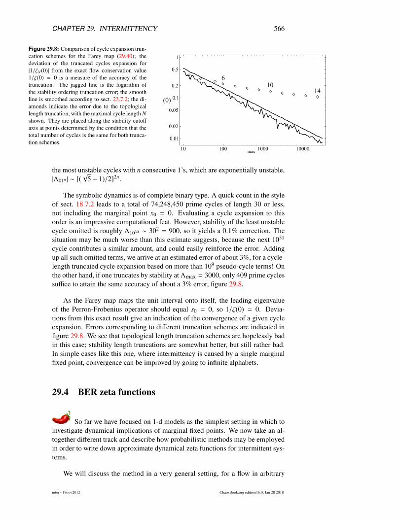
Figure 29.8: Comparison of cycle expansion trun-cation schemes for the Farey map (29.40); thedeviation of the truncated cycles expansion for|1/ζN(0)| from the exact flow conservation value1/ζ(0) = 0 is a measure of the accuracy of thetruncation. The jagged line is the logarithm ofthe stability ordering truncation error; the smoothline is smoothed according to sect. 23.7.2; the di-amonds indicate the error due to the topologicallength truncation, with the maximal cycle length Nshown. They are placed along the stability cutoff

axis at points determined by the condition that thetotal number of cycles is the same for both trunca-tion schemes.

10

10 100 1000 10000

0.01

0.02

0.05

0.1

0.2

0.5

1

6

14

(0)

max

the most unstable cycles with n consecutive 1’s, which are exponentially unstable,|Λ01n | ∼ [(

√5 + 1)/2]2n.

The symbolic dynamics is of complete binary type. A quick count in the styleof sect. 18.7.2 leads to a total of 74,248,450 prime cycles of length 30 or less,not including the marginal point x0 = 0. Evaluating a cycle expansion to thisorder is an impressive computational feat. However, stability of the least unstablecycle omitted is roughly Λ1030 ∼ 302 = 900, so it yields a 0.1% correction. Thesituation may be much worse than this estimate suggests, because the next 1031

cycle contributes a similar amount, and could easily reinforce the error. Addingup all such omitted terms, we arrive at an estimated error of about 3%, for a cycle-length truncated cycle expansion based on more than 109 pseudo-cycle terms! Onthe other hand, if one truncates by stability at Λmax = 3000, only 409 prime cyclessuffice to attain the same accuracy of about a 3% error, figure 29.8.

As the Farey map maps the unit interval onto itself, the leading eigenvalueof the Perron-Frobenius operator should equal s0 = 0, so 1/ζ(0) = 0. Devia-tions from this exact result give an indication of the convergence of a given cycleexpansion. Errors corresponding to different truncation schemes are indicated infigure 29.8. We see that topological length truncation schemes are hopelessly badin this case; stability length truncations are somewhat better, but still rather bad.In simple cases like this one, where intermittency is caused by a single marginalfixed point, convergence can be improved by going to infinite alphabets.

29.4 BER zeta functions

So far we have focused on 1-d models as the simplest setting in which toinvestigate dynamical implications of marginal fixed points. We now take an al-together different track and describe how probabilistic methods may be employedin order to write down approximate dynamical zeta functions for intermittent sys-tems.

We will discuss the method in a very general setting, for a flow in arbitrary



dimension. The key idea is to introduce a surface of section P such that all tra-jectories traversing this section will have spent some time both near the marginalstable fixed point and in the chaotic phase. An important quantity in what followsis (3.7), the first return time τ(x), or the time of flight of a trajectory starting inx to the next return to the surface of section P. The period of a periodic orbit pintersecting the P section np times is

Tp =

np−1∑k=0

τ( f k(xp)),

where f (x) is the Poincaré map, and xp ∈ P is a periodic point. The dynamicalzeta function (22.11)

1/ζ(z, s, β) =∏

p

(1 −

znpeβAp−sTp

|Λp|

), Ap =

np−1∑k=0

a( f k(xp)), (29.41)

associated with the observable a(x) captures the dynamics of both the flow and thechapter 20

Poincaré map. The dynamical zeta function for the flow is obtained as 1/ζ(s, β) =

1/ζ(1, s, β), and the dynamical zeta function for the discrete time Poincaré map is1/ζ(z, β) = 1/ζ(z, 0, β).

Our basic assumption will be probabilistic. We assume that the chaotic in-terludes render the consecutive return (or recurrence) times T (xi), T (xi+1) and ob-servables a(xi), a(xi+1) effectively uncorrelated. Consider the quantity eβA(x0,n)−sT (x0,n)

averaged over the surface of section P. With the above probabilistic assumptionthe large n behavior is

〈eβA(x0,n)−sT (x0,n)〉P ∼

(∫P

eβa(x)−sτρ(x)dx)n

,

where ρ(x) is the invariant density of the Poincaré map. This type of behavior isequivalent to there being only one zero z0(s, β) =

∫eβa(x)−sτ(x)ρ(x)dx of 1/ζ(z, s, β)

in the z-β plane. In the language of Ruelle-Pollicott resonances this means thatthere is an infinite gap to the first resonance. This in turn implies that 1/ζ(z, s, β)may be written as

remark 20.1

1/ζ(z, s, β) = z −∫P

eβa(x)−sτ(x)ρ(x)dx ,

where we have neglected a possible analytic and non-zero prefactor. The dynam-ical zeta function of the flow is now

1/ζ(s, β) = 1/ζ(1, s, β) = 1 −∫P

eβa(x)ρ(x)e−sτ(x)dx . (29.42)

Normally, the best one can hope for is a finite gap to the leading resonance ofthe Poincaré map. with the above dynamical zeta function only approximativelyvalid. As it is derived from an approximation due to Baladi, Eckmann, and Ruelle,we shall refer to it as the BER zeta function 1/ζBER(s, β) in what follows.

A central role is played by the probability distribution of return times

ψ(τ) =

∫P

δ(τ − τ(x))ρ(x)dx



The BER zeta function at β = 0 is then given in terms of the Laplace transformexercise 24.6

of this distribution

1/ζBER(s) = 1 −∫ ∞

0ψ(τ)e−sτdτ.

exercise 29.5

example 29.1

p. 572

example 29.2

p. 572

It may seem surprising that the BER approximation produces exact results inthe two examples above. The reason for this peculiarity is that both these systemsare piecewise linear and have complete Markov partitions. As long as the mapis piecewise linear and complete, and the probabilistic approximation is exactlyfulfilled, the cycle expansion curvature terms vanish. The BER zeta function andthe fundamental part of a cycle expansion discussed in sect. 23.1.1 are indeedintricately related, but not identical in general. In particular, note that the BER zetafunction obeys the flow conservation sum rule (23.17) by construction, whereasthe fundamental part of a cycle expansion as a rule does not.

Résumé

The presence of marginally stable fixed points and cycles changes the analyticstructure of dynamical zeta functions and the rules for constructing cycle ex-pansions. The marginal orbits have to be omitted, and the cycle expansionsnow need to include families of infinitely many longer and longer unstable or-bits which accumulate toward the marginally stable cycles. Correlations for suchnon-hyperbolic systems may decay algebraically with the decay rates controlledby the branch cuts of dynamical zeta functions. Compared to pure hyperbolicsystems, the physical consequences are drastic: exponential decays are replacedby slow power-law decays, and transport properties, such as the diffusion maybecome anomalous.

Commentary

Remark 29.1. What about the evolution operator formalism? The main virtue ofevolution operators was their semigroup property (20.26). This was natural for hyper-bolic systems where instabilities grow exponentially, and evolution operators capture thisbehavior due to their multiplicative nature. Whether the evolution operator formalism isa good way to capture the slow, power law instabilities of intermittent dynamics is lessclear. The approach taken here leads us to a formulation in terms of dynamical zeta func-tions rather than spectral determinants, circumventing evolution operators altogether. It isnot known if the spectral determinants formulation would yield any benefits when appliedto intermittent chaos. Some results on spectral determinants and intermittency can be



found in ref. [24]. A useful mathematical technique to deal with isolated marginally sta-ble fixed point is that of inducing, that is, replacing the intermittent map by a completelyhyperbolic map with infinite alphabet and redefining the discrete time; we have used thismethod implicitly by changing from a finite to an infinite alphabet. We refer to refs. [13,21, 22] for detailed discussions of this technique, as well as applications to 1-dimensionalmaps.

Remark 29.2. Intermittency. Intermittency was discovered by Manneville andPomeau [15] in their study of the Lorenz system. They demonstrated that in neighbor-hood of parameter value rc = 166.07 the mean duration of the periodic motion scales as(r − rc)1/2. In ref. [20] they explained this phenomenon in terms of a 1-dimensional map(such as (29.1)) near tangent bifurcation, and classified possible types ofintermittency.

Piecewise linear models like the one considered here have been studied by Gaspardand Wang [9, 26, 27]. The escape problem has here been treated following ref. [6], re-summations following ref. [5]. The proof of the bound (29.27) is given in P. Dahlqvist’snotes, see ChaosBook.org/extras/PDahlqvistEscape.pdf.

Farey map (29.40) has been studied widely in the context of intermittent dynamics,for example in refs. [1, 7, 16–19, 24]. The Fredholm determinant and the dynamicalzeta functions for the Farey map (29.40) and the related Gauss shift map (19.47) havebeen studied by Mayer [16]. He relates the continued fraction transformation to the Rie-mann zeta function, and constructs a Hilbert space on which the evolution operator isself-adjoint, and its eigenvalues are exponentially spaced, just as for the dynamical zetafunctions [23] for “Axiom A" hyperbolic systems.

Remark 29.3. Tauberian theorems. In this chapter we used Tauberian theorems forpower series and Laplace transforms: Feller’s monograph [8] is a highly recommendedintroduction to these methods.

Remark 29.4. Probabilistic methods, BER zeta functions. Probabilistic descriptionof intermittent chaos was introduced by Geisal and Thomae [11]. The BER approximationstudied here is inspired by Baladi, Eckmann and Ruelle [2], with further developments inrefs. [3, 4].

References

[1] R. Artuso, E. Aurell, and P. Cvitanovic, “Recycling of strange sets: II. Ap-plications”, Nonlinearity 3, 361–386 (1990).

[2] V. Baladi, J.-P. Eckmann, and D. Ruelle, “Resonances for intermittent sys-tems”, Nonlinearity 2, 119–135 (1989).

[3] P. Dahlqvist, “Determination of resonance spectra for bound chaotic sys-tems”, J. Phys. A 27, 763–785 (1994).

[4] P. Dahlqvist, “Approximate zeta functions for the Sinai billiard and relatedsystems”, Nonlinearity 8, 11 (1995).

[5] P. Dahlqvist, “Computing the topological pressure for intermittent maps”,J. Phys. A 30, L351–L358 (1997).


http://ChaosBook.org/extras/PDahlqvistEscape.pdf

http://dx.doi.org/10.1088/0951-7715/3/2/006

http://dx.doi.org/10.1088/0951-7715/3/2/006

http://dx.doi.org/10.1088/0951-7715/3/2/006

http://stacks.iop.org/0951-7715/2/i=1/a=007



http://dx.doi.org/10.1088/0305-4470/27/3/020

http://dx.doi.org/10.1088/0305-4470/27/3/020

http://dx.doi.org/10.1088/0305-4470/27/3/020

http://dx.doi.org/10.1088/0951-7715/8/1/002

http://dx.doi.org/10.1088/0951-7715/8/1/002

http://dx.doi.org/10.1088/0951-7715/8/1/002

http://dx.doi.org/10.1088/0305-4470/30/11/002

http://dx.doi.org/10.1088/0305-4470/30/11/002


[6] P. Dahlqvist, “Escape from intermittent repellers: Periodic orbit theory forcrossover from exponential to algebraic decay”, Phys. Rev. E 60, 6639–6644 (1999).

[7] C. P. Dettmann and P. Cvitanovic, “Cycle expansions for intermittent diffu-sion”, Phys. Rev. E 56, 6687–6692 (1997).

[8] W. Feller, An Introduction to Probability Theory and Its Applications, 2nd ed.(Wiley, 1971).

[9] P. Gaspard and X.-J. Wang, “Sporadicity: Between periodic and chaoticdynamical behaviors”, Proc. Natl. Acad. Sci. USA 85, 4591–4595 (1988).

[10] T. Geisel and J. Nierwetberg, “Onset of diffusion and universal scaling inchaotic systems”, Phys. Rev. Lett. 48, 7 (1982).

[11] T. Geisel and S. Thomae, “Anomalous diffusion in intermittent chaotic sys-tems”, Phys. Rev. Lett. 52, 1936 (1984).

[12] S. Grossmann and H. Fujisaka, “Diffusion in discrete nonlinear dynamicalsystems”, Phys. Rev. A 26, 1779–1782 (1982).

[13] S. Isola, “Renewal sequences and intermittency”, J. Stat. Phys. 97, 263–280(1999).

[14] R. Lombardi, Laurea thesis, MA thesis (Universitá degli studi di Milano,1993).

[15] P. Manneville and Y. Pomeau, “Intermittency and the Lorenz model”, Phys.Lett. A 75, 1–2 (1979).

[16] D. H. Mayer, “On a ζ function related to the continued fraction transforma-tion”, Bull. Soc. Math. Fr. 104, 195–203 (1976).

[17] D. H. Mayer, The Ruelle-Araki Transfer Operator in Classical StatisticalMechanics (Springer, Berlin, 1980).

[18] D. H. Mayer, “Continued fractions and related transformations”, in ErgodicTheory, Symbolic Dynamics, and Hyperbolic Spaces, edited by T. Bedford,M. Keane, and C. Series (Oxford Univ. Press, Oxford, 1991).

[19] D. Mayer and G. Roepstorff, “On the relaxation time of Gauss’s continued-fraction map I. The Hilbert space approach (Koopmanism)”, J. Stat. Phys.47, 149–171 (1987).

[20] Y. Pomeau and P. Manneville, “Intermittent transition to turbulence in dis-sipative dynamical systems”, Commun. Math. Phys. 74, 189 (1980).

[21] T. Prellberg, Maps of the interval with indifferent fixed points: thermody-namic formalism and phase transitions, PhD thesis (Virginia PolytechnicInst., 1991).

[22] T. Prellberg and J. Slawny, “Maps of intervals with indifferent fixed points:Thermodynamic formalism and phase transitions”, J. Stat. Phys. 66, 503–514 (1992).

[23] D. Ruelle, “Zeta-functions for expanding maps and Anosov flows”, Inv.Math. 34, 231–242 (1976).

[24] H. H. Rugh, “Intermittency and regularized Fredholm determinants”, Inv.Math. 135, 1–24 (1999).


http://dx.doi.org/10.1103/PhysRevE.60.6639







http://dx.doi.org/10.2307/1267002

http://www.pnas.org/content/85/13/4591.abstract



http://dx.doi.org/10.1103/PhysRevLett.48.7






http://dx.doi.org/10.1103/PhysRevA.26.1779



http://dx.doi.org/10.1023/A:1004623303471

http://dx.doi.org/10.1023/A:1004623303471

http://dx.doi.org/10.1023/A:1004623303471

http://dx.doi.org/10.1016/0375-9601(79)90255-X

http://dx.doi.org/10.1016/0375-9601(79)90255-X

http://dx.doi.org/10.1016/0375-9601(79)90255-X

http://www.numdam.org/item?id=BSMF_1976__104__195_0



http://dx.doi.org/10.1007/bfb0017919

http://dx.doi.org/10.1007/bfb0017919

http://books.google.com/books?vid=ISBN9780198533900

http://dx.doi.org/10.1007/BF01009039

http://dx.doi.org/10.1007/BF01009039

http://dx.doi.org/10.1007/BF01009039

http://dx.doi.org/10.1007/BF01009039

http://dx.doi.org/10.1007/BF01197757

http://dx.doi.org/10.1007/BF01197757

http://dx.doi.org/10.1007/BF01197757

http://dx.doi.org/10.1007/BF01060077

http://dx.doi.org/10.1007/BF01060077

http://dx.doi.org/10.1007/BF01060077

http://dx.doi.org/10.1007/BF01060077

http://dx.doi.org/10.1007/bf01403069

http://dx.doi.org/10.1007/bf01403069

http://dx.doi.org/10.1007/bf01403069

http://dx.doi.org/10.1007/s002220050277

http://dx.doi.org/10.1007/s002220050277

http://dx.doi.org/10.1007/s002220050277


[25] M. Schell, S. Fraser, and R. Kapral, “Diffusive dynamics in systems withtranslational symmetry: A one–dimensional–map model”, Phys. Rev. A 26,504–521 (1982).

[26] X.-J. Wang, “Abnormal fluctuations and thermodynamic phase transitionsin dynamical systems”, Phys. Rev. A 39, 3214–3217 (1989).

[27] X.-J. Wang, “Statistical physics of temporal intermittency”, Phys. Rev. A40, 6647–6661 (1989).













29.5 Examples

Example 29.1. Return times for the Bernoulli map. For the Bernoulli shift map(28.21)

x 7→ f (x) = 2x mod 1,

one easily derives the distribution of return times

ψn =12n n ≥ 1.

The BER zeta function becomes (by the discrete Laplace transform (21.8))

1/ζBER(z) = 1 −∞∑

n=1

ψnzn = 1 −∞∑

n=1

zn

2n

=1 − z

1 − z/2= ζ−1(z)/(1 − z/Λ0) . (29.43)

Thanks to the uniformity of the piecewise linear map measure (19.39) the “approximate"click to return: p. 568

zeta function is in this case the exact dynamical zeta function, with the periodic point 0pruned.

Example 29.2. Return times for the model of sect. 29.2.1. For the toy model ofsect. 29.2.1 one gets ψ1 = |M1|, and ψn = |Mn|(1−b)/(1−a), for n ≥ 2, leading to a BERzeta function

1/ζBER(z) = 1 − z|M1| −

∞∑n=2

|Mn|zn,

which again coincides with the exact result, (29.10).click to return: p. 568


EXERCISES 573

Exercises

29.1. Integral representation of Jonquière functions.Check the integral representation

J(z, α) =z

Γ(α)

∫ ∞

0dξ

ξα−1

eξ − zfor α > 0 .

(29.44)

Note how the denominator is connected to Bose-Einstein distribution. Compute J(x + iε) − J(x − iε) fora real x > 1.

29.2. Power law correction to a power law. Expand(29.20) further and derive the leading power law correc-tion to (29.23).

29.3. Power-law fall off. In cycle expansions the stabilitiesof orbits do not always behave in a geometric fashion.Consider the map f

0.2 0.4 0.6 0.8 1

0.2

0.4

0.6

0.8

1

This map behaves as f → x as x → 0. Define a sym-bolic dynamics for this map by assigning 0 to the pointsthat land on the interval [0, 1/2) and 1 to the points thatland on (1/2, 1]. Show that the stability of orbits thatspend a long time on the 0 side goes as n2. In particular,show that

Λ 00···0︸︷︷︸n

1 ∼ n2

29.4. Power law fall-off of Floquet multipliers in the sta-

dium billiard. From the cycle expansionspoint of view, the most important consequence of theshear in Jn for long sequences of rotation bounces nk in(9.13) is that the Λn grows only as a power law in num-ber of bounces:

Λn ∝ n2k . (29.45)

Check.

29.5. Probabilistic zeta function for maps. Derive theprobabilistic zeta function for a map with recurrence dis-tribution ψn.

29.6. Accelerated diffusion. Consider a map h, such thath = f , but now running branches are turner into stand-ing branches and vice versa, so that 1, 2, 3, 4 are stand-ing while 0 leads to both positive and negative jumps.Build the corresponding dynamical zeta function andshow that

σ2(t) ∼

t for α > 2t ln t for α = 2t3−α for α ∈ (1, 2)t2/ ln t for α = 1t2 for α ∈ (0, 1)

29.7. Anomalous diffusion (hyperbolic maps). Anoma-lous diffusive properties are associated to deviationsfrom linearity of the variance of the phase variable weare looking at: this means the diffusion constant (20.40)either vanishes or diverges. We briefly illustrate in thisexercise how the local local properties of a map are cru-cial to account for anomalous behavior even for hyper-bolic systems.Consider a class of piecewise linear maps, relevant tothe problem of the onset of diffusion, defined by

fε(x) =

Λx for x ∈[0, x+

1

]a − Λε,γ|x − x+| for x ∈

[x+

1 , x+2

]1 − Λ′(x − x+

2 ) for x ∈[x+

2 , x−1

]1 − a + Λε,γ|x − x−| for x ∈

[x−1 , x

−2

]1 + Λ(x − 1) for x ∈

[x−2 , 1

]where Λ = (1/3 − ε1/γ)−1, Λ′ = (1/3 − 2ε1/γ), Λε,γ =

ε1−1/γ, a = 1+ε, x+ = 1/3, x+1 = x+−ε1/γ, x+

2 = x++ε1/γ,and the usual symmetry properties (24.22) are satisfied.Thus this class of maps is characterized by two escap-ing windows (through which the diffusion process maytake place) of size 2ε1/γ: the exponent γ mimicks the or-der of the maximum for a continuous map, while piece-wise linearity, besides making curvatures vanish andleading to finite cycle expansions, prevents the appear-ance of stable cycles. The symbolic dynamics is eas-ily described once we consider a sequence of param-eter values {εm}, where εm = Λ−(m+1): we then par-tition the unit interval though the sequence of points0, x+

1 , x+, x+

2 , x−1 , x

−, x−2 , 1 and label the correspondingsub–intervals 1, sa, sb, 2, db, da, 3: symbolic dynamics is

exerInter - 6jun2003 ChaosBook.org edition16.0, Jan 28 2018

EXERCISES 574

described by an unrestricted grammar over the followingset of symbols

{1, 2, 3, s# ·1i, d# ·3k} # = a, b i, k = m,m+1,m+2, . . .

This leads to the following dynamical zeta function:

ζ−10 (z, α) = 1−

2zΛ−

zΛ′−4 cosh(α)ε1/γ−1

mzm+1

Λm

(1 −

zΛ

)−1

from which, by (24.8) we get

D =2ε1/γ−1

m Λ−m(1 − 1/Λ)−1

1 − 2Λ− 1

Λ′− 4ε1/γ−1

m

(m+1

Λm(1−1/Λ) + 1Λm+1(1−1/Λ)2

)

(29.46)

The main interest in this expression is that it allows ex-ploring how D vanishes in the ε 7→ 0 (m 7→ ∞) limit: asa matter of fact, from (29.46) we get the asymptotic be-havior D ∼ ε1/γ, which shows how the onset of diffusionis governed by the order of the map at its maximum.

Remark 29.5. Onset of diffusion for continuous maps.The zoology of behavior for continuous maps at the on-set of diffusion is described in refs. [10, 12, 25]: ourtreatment for piecewise linear maps was introduced inref. [14].

exerInter - 6jun2003 ChaosBook.org edition16.0, Jan 28 2018

intermittency - chaosbook.orgchaosbook.org/chapters/inter.pdf · n the theory of chaotic dynamics...

Documents