intermediate excel 2007 - the college of saint roseits.strose.edu/userfiles/intermediate excel...

Revised: 11/6/08

Intermediate Excel 2007

Table of Contents Overview..........................................................................................................................................1

Objectives ........................................................................................................................................1

Worksheet Operations....................................................................................................................2Activate a Worksheet.................................................................................................................................. 2Insert a Worksheet ...................................................................................................................................... 2Rename a Worksheet .................................................................................................................................. 3Change Tab Color....................................................................................................................................... 4Delete a Worksheet..................................................................................................................................... 5Move or Copy Worksheets ......................................................................................................................... 6Grouping Worksheets ................................................................................................................................. 9Ungroup Worksheets ................................................................................................................................ 11

Formulas........................................................................................................................................12Order of Operations .................................................................................................................................. 13AutoSum ................................................................................................................................................... 16

Cell References..............................................................................................................................19Relative ..................................................................................................................................................... 19Absolute .................................................................................................................................................... 20Mixed ........................................................................................................................................................ 20

Functions .......................................................................................................................................22Insert Function .......................................................................................................................................... 22The Function Arguments Dialog Box....................................................................................................... 23Frequently used Functions ........................................................................................................................ 24

Links...............................................................................................................................................25

Exercise - Links.............................................................................................................................26

3-Dimensional References ............................................................................................................29Create a 3-D Reference............................................................................................................................. 29

Conditional Formatting................................................................................................................31

Range Finder.................................................................................................................................34

Auto Calculate...............................................................................................................................35

Freeze Panes ..................................................................................................................................36Clear Frozen Titles.................................................................................................................................... 37

Error Checking .............................................................................................................................38

Summary .......................................................................................................................................40

Information Technology Services The College of Saint Rose

Intermediate Excel 2007 1

Overview

This course focuses on Intermediate Topics in Excel. In this class you will learn how to work with multiple worksheets, create formulas, use functions, link data to other worksheets, and use the Auto Calculate feature and the Range Finder.

The Excel file that will be used for practice is called Athletics Budget and contains six worksheets: Volleyball, Golf, Baseball, Softball, Summary, Expenses.

Objectives

Work with multiple worksheets

Create formulas

Differentiate between relative and absolute cell references

Use built-in functions

Link data

Create 3-dimensional formulas

Use Range Finder

Apply conditional formatting

Error checking

View Auto Calculate feature

Freeze Panes



Worksheet Operations

By default Excel includes three worksheets to start, but sometimes you will need more or less sheets. For example, if you have a budget with a sheet for every month and then a summary sheet that totals your yearly budget, then you need 13 sheets in the workbook. You will probably want to rename the sheets from their default sheet1, sheet2 and sheet3 to more meaningful names, such as the months. One way these operations can be easily performed is to right click on a sheet tab and make a selection from the shortcut menu.

Activate a Worksheet Open the workbook named Athletics Budget.xls in My Documents.

1. Just Click on the tab of the Worksheet that you want to work on.

Insert a Worksheet 1. Click on the worksheet tab where you want to insert the new worksheet.

2. In the cells group from the Home tab, click Insert Sheet.

OR

3. Right-click on the worksheet tab.

4. Select Insert from the shortcut menu.



5. Select worksheet from the insert dialog box.

6. A new worksheet tab will appear before the worksheet tab you selected.

7. You can insert a worksheet at the end of the workbook by clicking the Insert Worksheet tab located to the right of the last sheet tab in the workbook.

Rename a Worksheet Worksheet names cannot exceed 31 characters long, including blank spaces.

It cannot contain the characters : ? */ \ or square brackets.

1. Double-click on the tab that you want to rename.

2. Type in the new name.

3. Click off the sheet tab to enter.



OR

1. Right-click on the sheet tab that you want to rename.

2. Choose rename from the shortcut menu.

3. Type in the new name.

4. Click off the sheet tab to enter.

Change Tab Color Another new feature in Excel 2007 is you can change the sheet tab color.

From the shortcut menu choose Tab Color and select a color from the color palette.



Delete a Worksheet 1. Select the worksheet that you want to delete.

2. Right-click on the sheet tab that you want to rename.

3. Choose Delete from the shortcut menu.

OR

4. On the Home tab in the cells group, click Delete Sheet from the delete drop-down menu.



Move or Copy Worksheets You can move or copy a whole worksheet to another location in a workbook or to another open workbook. However, be careful when you move or copy a worksheet. Calculations or charts that are based on worksheet data might become inaccurate if you move the worksheet. Similarly, if a moved or copied worksheet is inserted between sheets that are referred to by a 3-D formula reference (A reference to a range that spans two or more worksheets in a workbook) data on that worksheet might be unexpectedly included in the calculation.

You can also use the Cut or Copy commands to move or copy all or part of the data in a worksheet to another worksheet in the same workbook or another workbook. You can also drag worksheet data between workbook windows or workbooks that are open in separate instances of Excel.

Drag and Drop Method

1. Click on the worksheet tab that you want to move.

2. Click and hold the mouse button down, an arrow with a miniature sheet of paper

appears. Drag and drop it to the desired location.

1. To create a copy, press the Ctrl key as you drag and drop the sheet tab.

2. Release the mouse button, and then release the Ctrl key.



Move or Copy Dialog box

1. Select (Click on the tab of) the worksheet that you want to move or copy.

2. On the Home tab, in the Cells group, click Format, and then under Organize Sheets, click Move or Copy Sheet.

Note: You can also right-click a selected sheet tab, and then click Move or Copy from the shortcut menu.



The Move or Copy dialog box opens, as shown below.

3. In the ‘To book’ drop down list, select the workbook to which you want to move or copy the selected sheets.

• Or click (new book) to move or copy the selected sheets to a new workbook.

4. In the ‘Before sheet’ list select the sheet that you want the active worksheet to be inserted in front of, or click move to end to insert the sheet after the last sheet in the workbook and before the Insert Worksheet tab.

• To copy of the sheet, select the Create a copy check box.

5. Click on OK. The worksheet will be moved or copied to the new location.

Note: When you create a copy of the worksheet, the worksheet is duplicated in the destination workbook. When you move a worksheet, the worksheet is removed from the original workbook and appears in the destination workbook only.

You can Move/Copy the worksheet to a New workbook or to another existing open workbook.

Click to create a copy



Grouping Worksheets Grouping worksheets enables you to simultaneously perform tasks on all the worksheets.

Note: If you use this feature, the layout or structure of each of the worksheets needs to be identical.

Select multiple worksheets to group them.

To group adjacent worksheets

1. Activate a worksheet, press and hold the SHIFT key.

2. Click on the worksheet tab at the end of the group.

To group non-adjacent worksheets

1. Activate a worksheet, press and hold the CTRL key.

2. Click on the worksheet tabs you want to group.

Exercise

1. Group the worksheets Volleyball, Baseball, Softball, and Golf.

2. Notice that the Excel title bar displays athletics budget [Group] to indicate that there are grouped worksheets.



3. Select the cell range C10:C37. Format the cells as currency with no decimal places. Choose the $ symbol. Click OK.

4. Select the cell rangeA1:C8. On the ‘Home’ tab select the Fill Color button drop down arrow and choose a Fill color of your choice.

5. Click on another worksheet tab in the group. Notice that the formatting changes were applied to all the worksheets that were grouped!



Ungroup Worksheets 1. Right click on one of the worksheet tabs that are grouped.

2. Choose Ungroup Sheets from the shortcut menu.

3. You can now treat worksheets individually.



Formulas

A Formula is a set of mathematical instructions that perform calculations. Formulas can contain numbers, text, cell references, other formulas, and operators.

Formulas perform operations such as addition and multiplication. Operators are symbols used in formulas to perform mathematical functions.

Formulas begin with an equal sign (=).

Create formulas using cell references rather than numbers. This way if the value changes in a cell referenced by the formula, the formula automatically recalculates and updates the result.

Point and click on cell references used in the formula (instead of typing the cell address) and type the operators to specify the types of calculations to perform.

Formulas can refer to other cells on the same worksheet, cells on other sheets in the same workbook, or cells on sheets in other workbooks.



Order of Operations Excel performs calculations using the mathematical order of operations. This is the sequence or order in which computations are performed. Certain operators have a higher precedence than other operators. If a formula contains operators with the same precedence such as addition and subtraction, they are evaluated from left to right. The order of precedence can be overridden by enclosing the operation you want performed first in parentheses.

The table below displays operators, their symbols and the order in which operations are performed in a formula or equation.

A good mnemonic to use to remember the order of operations is:

Please Excuse My Dear Aunt Sally

Parentheses, Exponents, Multiplication, Division, Addition, Subtraction

You can override the normal order of operations by using parenthesis. Whatever is enclosed in parentheses is performed first!

Order Operator Description

1 ( ) Parenthesis

2 ^ Exponents

3 * Multiplication

4 / Division

5 + Addition

6 - Subtraction

7 =, <, <=, >, >=, <> Comparison (equal to, less than, less than or equal to, greater than, greater than or equal to, not equal to)



Exercise – Order of Operations

Example 1

What is the correct answer below?

6+2*7 = 56

Or

6+2*7 = 20

It is easy to think that you calculate this in the order it is encountered (from left to right) in which the answer would appear to be 56, but this is incorrect. The order of operations dictates that multiplication is performed before addition, therefore the answer is 20.

You can also check your answers by manually entering the formula into Excel. Start with the = sign, type your equation and press enter. Obtain the answer for the first example. Test this out in any cell in the Worksheet.

Type in =6+2*7.

Press Enter.

Example 2

How would Excel evaluate the following equation?

=36+4/2

Division has a higher priority (order of operation) than addition; therefore, 4/2 would be

performed first then the dividend would be added to 36. The answer is 38.

If the desired operation is 36+4 then divided by 2, it would be necessary to enclose

(36+4) in parentheses. =(36+4)/2. In this form, the answer would be 20.

Tip: It is better to use parenthesis in your equations to avoid any confusion =36+(4/2).



Exercise

In the Expenses worksheet, enter a formula that will add the total expenses for the month of January.

Use Pointing to enter a Formula

Rather than typing in cell references for a formula you enter them by selecting the worksheet cells. As you enter the formula, point to the cell references for the formula.

Notice that Excel helps you keep track of the cell references by identifying the referenced cell with a colored border and using the same color for the cell address in the formula.

1. Click in cell B10. To begin a formula type an equal ( = ) symbol. 2. Point to cell B4. 3. Type the addition symbol ( + ). 4. Point to cell B5 5. Type the addition symbol ( + ). 6. Point to cell B6 7. Type the addition symbol ( + ). 8. Point to cell B7 9. Type the addition symbol ( + ). 10. Point to cell B8 11. Type the addition symbol ( + ). 12. Point to cell B9 13. Type the addition symbol ( + ).

14. Press Enter to complete the formula. The total is shown below.

Well, this is a very cumbersome and an inefficient way to add an entire row or column of numbers. Fortunately, Excel provides the Auto Sum function to perform this calculation.



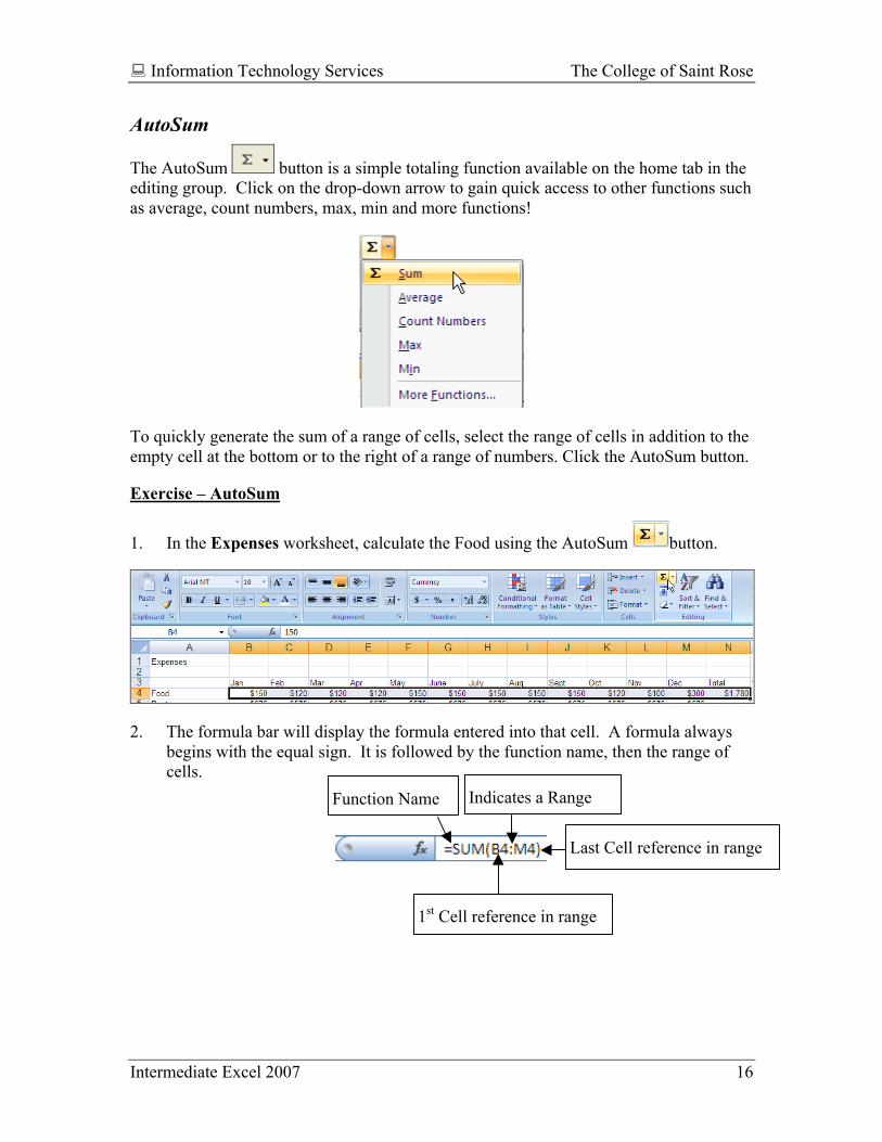
AutoSum

The AutoSum button is a simple totaling function available on the home tab in the editing group. Click on the drop-down arrow to gain quick access to other functions such as average, count numbers, max, min and more functions!

To quickly generate the sum of a range of cells, select the range of cells in addition to the empty cell at the bottom or to the right of a range of numbers. Click the AutoSum button.

Exercise – AutoSum

1. In the Expenses worksheet, calculate the Food using the AutoSum button.

2. The formula bar will display the formula entered into that cell. A formula always begins with the equal sign. It is followed by the function name, then the range of cells.

Indicates a Range Function Name

1st Cell reference in range

Last Cell reference in range



AutoFill a Formula

You could copy and paste the formula and format to the other cells in the row. But, AutoFill is a faster method to quickly copy formulas and formats to adjacent cells.

Exercise – AutoFill

Calculate the total expenses for each row. Use the AutoFill feature to expedite the process.

1. Select the cell or range of cells that contain the formula that you want to fill into adjacent cells.

2. Drag the fill handle across the cells that you want to fill. (The fill handle is the small black square in the lower-right corner of the selection. When you point to the fill handle, the pointer changes to a black cross.)

3. Drag across the cells that you want to fill.

Mouse Pointer changes to a black cross Fill Handle is

a black square



4. When using the AutoFill feature, the AutoFill Options smart tag will appear under the lower right hand corner of the last AutoFill entry. This smart tag gives you additional control over the AutoFill options.

5. For example, you can choose to Copy Cells, Fill Formatting Only or Fill Without Formatting.

Copies just the formula without the formatting

Copies both the formula and the formatting

Copies just the formatting of the cell



Cell References

Formulas can contain relative, absolute or mixed cell references.

Relative By default, copied formulas use relative references. Relative references are interpreted in relation or relative to the location of the cell containing the formula. When a formula is copied from one cell to another, the result is not an exact copy or duplicate of the value. Excel copies the formula using relative cell references and automatically adjusts the formula to reflect the new cell location to which the formula is copied.

The example below illustrates how a relative reference in a formula changes when the formula is copied to another range. When the formula for cell N4 is copied to the other cells in the column, the formula is a relative cell reference and sums everything in row 5, even though we copied the formula from row 4. This is the beauty of relative cell references. The formula will adjust itself to the new location to which the formula is copied.

Exercise

1. AutoSum the total expenses for the month of January.

2. Copy (Auto fill) the formula across to the other months. Notice how Excel copies the

formula relatively into the adjacent cells.



Absolute An absolute cell reference in a formula will always refer to a specific fixed cell address. If you copy the formula across rows or down columns, an absolute reference does not adjust.

By default, Excel uses relative cell references. If you need an absolute cell reference in your formula, insert a dollar sign $ symbol in front of the column letter and row number. For example, to make cell B12 an absolute cell reference, it would look like $B$12.

Tip: Use the F4 function key while editing the formula to easily insert the $ symbol and make it absolute.

Mixed A mixed cell reference has either an absolute column and relative row, or absolute row and relative column.

An absolute column reference takes the form of $A1, $A2, $A3 etc.

An absolute row reference takes the form of A$1, B$1, C$1, etc.

If you copy the formula across rows or down columns, the relative reference automatically adjusts, and the absolute reference does not adjust.

Tip: If you keep pressing the F4 key to cycle through the different variants. This is used to create mixed cell references.



Exercise

In the Expenses Worksheet calculate the projected increase and projected total.

1. In cell B13 calculate the projected increase. Multiply the total expenses for Jan in cell B10 by the projected increase of 5% in cell A12.

2. Copy the formula across to fill the row.

3. What were your results? Did you remember to refer to cell $A$12 as an absolute cell reference in your formula? If not your result will be $0.00. As the formula is copied, the absolute cell reference $A$12 stays the same, but all relative cell references (without $) automatically change relative to their location in the worksheet.

4. In cell B14 calculate the projected total by adding the projected increase to the total. Add cells B10+B13.

5. Copy the formula across to fill the row.

6. The results are shown below.



Functions

Functions are predefined formulas that perform many common analytical operations. Excel includes over 300 built-in functions. Functions are organized or grouped by category such as Financial, Statistical, Math&Trig.

Each built in Excel function requires specific information in a specific format. The insert function dialog box allows you to choose a function then prompts you for arguments (data) the function uses to perform the calculation.

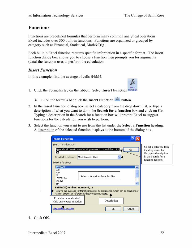
Insert Function In this example, find the average of cells B4:M4.

1. Click the Formulas tab on the ribbon. Select Insert Function .

OR on the formula bar click the Insert Function button. 2. In the Insert Function dialog box, select a category from the drop down list, or type a

description of what you want to do in the Search for a function box and click on Go. Typing a description in the Search for a function box will prompt Excel to suggest functions for the calculation you wish to perform.

3. Select the function you want to use from the list under the Select a Function heading. A description of the selected function displays at the bottom of the dialog box.

4. Click OK.

Description

Select a function from this list.

Provides more detailed Help on selected function

Select a category from the drop down list. Or type a description in the Search for a function textbox.



The Function Arguments Dialog Box The function arguments dialog box helps you enter cell references into a function or formula.

5. The Function Arguments dialog box will open.

6. Excel attempts to intuit the range of cells or data needed to complete the function. If the range indicated in the function arguments dialog box is not correct (as in this case) click and select the appropriate range of cells in the spreadsheet.

7. Click OK, to complete the function.

8. Copy the formula down to the remaining cells. You are done!

You can also click on the Collapse dialog box button and select the cell range.

Click the Expand dialog box button once the range is selected. Click OK.



Frequently used Functions A shortcut to built-in functions can be obtained on the formula bar.

1. Type and equal sign = to begin your formula. Notice in the Name text box displays commonly used functions.

2. Click on the function drop-down arrow and select the function you want from the list.

If the function you want is not listed, click on More Functions to open the Insert Function dialog box.

3. Select the range of cells.

4. Click OK or click on the checkmark on the formula bar to enter the function.



Links

You can refer to data in different worksheets and workbooks by linking. A link is a formula that refers to a cell or a range in another worksheet or workbook. A formula that contains references to cells in other sheets of a workbook allows you to use data from multiple sheets and to calculate new values based on this data.

Advantages

Linking data within your workbook saves you time - you do not have to re-enter the data. It ensures that your data is current and up-to-date. If the data in one sheet changes, the data in another sheet that is linked to it will automatically update to reflect those changes.

Reference Cells in other Worksheets

The syntax for a cell reference is shown below. While you may type references, it is much easier to enter them by pointing to the cells on the sheet which you want to refer to.

=Worksheet Name!Cell Address

The completed formula will display the worksheet name followed by an exclamation point and the cell or range reference. If a worksheet name contains a blank space in its name, then the worksheet name must be enclosed in single quotation marks.

Reference Cells in other Workbooks

You can refer to the contents of cells in another workbook by creating an external link or external reference. An external reference refers to a cell or range of cells on a worksheet in another Excel workbook. External references come in handy when working with data that spans across several other workbooks. For example, you may be trying to merge data from different departments into a summary workbook. In this case you have a source workbook (where the data originates) and a destination workbook. When the source workbook is changed you will not have to manually change the summary workbook. You will be prompted to update your links upon opening the destination file.

If calculations involve cell references in other workbooks, the format is as follows:

[Workbook Name]Worksheet Name!Cell Address



Exercise - Links

1. In the Athletics Budget workbook, open the Summary worksheet, select cell C10.

2. Start a formula by typing an equal sign =.

3. Point to the cell in the source worksheet that contains the data you want to refer to. In this example, click on the Volleyball worksheet and click on cell C10.

4. Press Enter. You are returned to the summary worksheet and the value is entered.

• Notice your formula. The formula in the summary worksheet indicates the worksheet name and the cell address to which it refers. If the data changes in the Volleyball worksheet, the data in the summary worksheet will update automatically.

5. Use the AutoFill feature to copy the formula down the rest of column C.



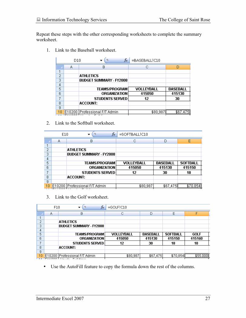
Repeat these steps with the other corresponding worksheets to complete the summary worksheet.

1. Link to the Baseball worksheet.

2. Link to the Softball worksheet.

3. Link to the Golf worksheet.

• Use the AutoFill feature to copy the formula down the rest of the columns.



• In cell G10 use the AutoSum feature to total the numbers in row 10.

• Copy the formula down the column.

• Lastly, create a mixed cell reference to calculate the Projected Total and copy the formula down the column.



3-Dimensional References

A worksheet formula that refers to the same cell or range of cells in other worksheets is called a three-dimensional (3-D) formula. It is often used to summarize data.

The format of a 3-D formula is shown below.

If a sheet is inserted or deleted, the range is automatically updated.

Create a 3-D Reference 1. Click the cell where you want to enter the function.

2. Select a function such as Sum.

3. Click the sheet tab for the first worksheet that you want to reference.

4. Hold down SHIFT and click the tab for the last worksheet that you want to reference.

5. Select the cell or range of cells that you want to reference.

6. Press ENTER to complete the formula.

Function name Last sheet in range

Cell Address

First sheet in range



Exercise – 3-D Formula

1. Click the cell where you want to enter the function. In the Athletics Budget workbook, open the 3D total worksheet, select cell C7.

2. Select the Sum function.

3. Click the first worksheet that you want to reference. In this example select the Volleyball sheet.

4. Hold down SHIFT and click the tab for the last worksheet that you want to reference. In this example select the Golf sheet.

5. Select Cell C10.

6. Press ENTER to complete the formula.

7. The 3-D reference is shown in the formula bar below. It includes sheet names and cell references.

8. Auto fill down to complete the column.



Conditional Formatting

Conditional formatting changes the appearance of a range of cells based on a condition you set. This allows you to highlight or emphasize certain values in the spreadsheet which make it easier to spot trends and analyze the information.

Excel has four conditional formats that can be applied: Highlighting, Data Bars, Color Scales and Icon Sets.

1. To apply conditional formatting, select the range of cells in your worksheet.

2. In the Style group on the Home tab, click Conditional Formatting.

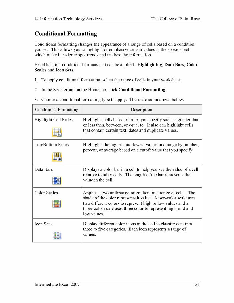
3. Choose a conditional formatting type to apply. These are summarized below.

Conditional Formatting Description

Highlight Cell Rules

Highlights cells based on rules you specify such as greater than or less than, between, or equal to. It also can highlight cells that contain certain text, dates and duplicate values.

Top/Bottom Rules

Highlights the highest and lowest values in a range by number, percent, or average based on a cutoff value that you specify.

Data Bars

Displays a color bar in a cell to help you see the value of a cell relative to other cells. The length of the bar represents the value in the cell.

Color Scales

Applies a two or three color gradient in a range of cells. The shade of the color represents it value. A two-color scale uses two different colors to represent high or low values and a three-color scale uses three color to represent high, mid and low values.

Icon Sets

Display different color icons in the cell to classify data into three to five categories. Each icon represents a range of values.



Exercise – Apply Top 10 Rule Conditional Format

1. In the 3-D total worksheet select the range C7:C33.

2. In the Style group on the Home tab, click the Conditional formatting button.

3. Choose the conditional formatting type to apply.

• In this example select Top/Bottom Rules → Top 10 items.

4. In the top 10 items dialog box you can select the formatting you want to apply for the top 10 items. In this example accept the default, (Light Red Fill with Dark Red Text) shown below.



5. The conditional format is applied to the top 10 values in the column as shown below.

Clear the Rules

6. In the Style group on the Home tab, click the Conditional Formatting button.

7. Click Clear Rules. Choose to Clear Rules from Selected Cells or Entire Sheet. The formatting is then removed.



Range Finder

Range Finder - A feature that helps you edit formulas by highlighting formula cell ranges in different colors. The Range Finder color-codes the formula cell references.

Turn on the Range Finder

1. Click in the formula bar or double click on the cell and the range finder highlights the formula cell ranges in different colors.

Exercise

1. In the summary worksheet, select cell H10.

2. Click in the formula bar and notice that the range finder highlights the formula cell ranges in different colors.

Notice the range finder highlights in color both the formula and around the formula cells.



Auto Calculate

The Auto Calculate feature instantly displays functions such as the sum, average, or

count (the number of numeric values in a selected range of cells). The Auto Calculate

function displays the results in the Auto Calculate area of the status bar.

To use Auto Calculate:

1. Select the desired range of cells. View the results in the status bar as shown below.

Customize Status Bar

2. Right click anywhere on the status bar.

3. Click in the Auto Calculate area on the Status Bar with the right mouse button.

4. From the menu select the desired options you want to appear on the status bar.

Auto Calculate Area



Freeze Panes

The Freeze Panes feature allows you to lock specific rows or columns in a worksheet so

they do not move when scrolling. You can freeze a specified row, column or both. For

example, you may want row or column labels to remain visible on the screen when you

scroll throughout the worksheet.

On the worksheet, do one of the following:

• To lock rows, select the row below the row or rows that you want to keep visible when you scroll.

• To lock columns, select the column to the right of the column or columns that you want to keep visible when you scroll.

• To lock both rows and columns, click the cell below and to the right of the rows and columns that you want to keep visible when you scroll.

1. On the View tab, in the Window group, click Freeze Panes.

2. Click Freeze Panes to lock a row or column, or to lock both rows and columns at the same time. To lock the first row only, click Freeze Top Row. To lock first column only, click Freeze First Column.

3. A solid line appears along the bottom of a row or right side of a frozen column. The frozen titles remain stationary when scrolling.



Exercise

1. In the Athletics Budget workbook, open the Summary worksheet, select cell C6.

2. On the View tab, in the Window group, click Freeze Panes.

3. Notice that a solid line appears along the bottom of a row and the right side of a frozen column. Scroll down or to the right and the frozen titles remain stationary!

Clear Frozen Titles When you freeze the top row, first column, or panes, the Freeze Panes option changes to Unfreeze Panes so that you can unlock any frozen rows or columns.

1. To unfreeze panes select Unfreeze Panes.

2. This clears the frozen panes (or titles).



Error Checking

Excel comes with an error checking feature that looks for the most common errors people make when creating formulas. These errors include the following:

Error Description

Evaluates to Error Value

This error catches formulas that divide by zero or that result in ‘not a number’ answers.

Text data with 2 digit years

This error message occurs when you use a two digit year in a formula. For example if you use 11/17/03, the program does not know if you mean 1903 or 2003 and will mark it as an error.

Number stored as text The information stored in the cell is in text format and cannot be used in a formula.

Inconsistent formula in region The references used in a formula are not consistent with the references used in adjacent formulas.

Formula omits cells in region

This error will occur if your formula refers to a range of cells, and adjacent cells are not included in the formula but contain data. For example, if you are summing data in a column and use the formula SUM(A3:A5) but cell A2 also contains data, Excel will mark this as a possible error.

Unlocked cells containing formula

It is possible to lock cells in Excel such that other users cannot change the formula. Users with permission to modify the workbook have to unlock the cell to change the formula. This error will appear when the user leaves a cell containing a formula unprotected.

Formula refers to empty cells This error informs the user that the formula includes cells that do not contain data.



Upon finding a potential error, an error value is displayed and/or Excel places a green triangle in the upper left-hand corner of the cell that may contain the error. Click in the cell and a smart tag will appear near the triangle. Click the smart tag to access a drop down menu that lists possible errors. It also allows the user to fix the error, access the topic on the help menu that discusses the error, ignore the error, or edit the formula.

You can turn off background error checking in Excel or reset any errors you have previously chosen to ignore by selecting Error Checking Options.

You can tell which rules are enabled based on whether or not a checkbox appears in the small box next to the rule. To disable a single rule, click on the box next to the rule. To re-enable the rule, click in the box again and a check mark will appear. Clicking on Reset Ignored Errors will reset any errors you chose to ignore using the Smart Tabs.

Potential Error

Turn on or off background checking.

Reset any errors you have previously chosen to ignore

Suggested Solution



Summary

You have completed the Intermediate Excel class. The main purpose of this class was to familiarize you with some of the timesaving features in Excel. You learned how to copy, move, delete, and group worksheets within a workbook. You worked with formulas, functions, and freeze panes. Conditional formatting was examined as well as some of the most common spreadsheet errors that occur when working with formulas. You also used the range finder to color code formula cell references, and quickly viewed the sum of a selected range using the Auto Calculate feature.