intergenerational occupational mobility in indiaftp.iza.org/dp7608.pdf · intergenerational...
TRANSCRIPT

DI
SC
US
SI
ON
P
AP
ER
S
ER
IE
S
Forschungsinstitut zur Zukunft der ArbeitInstitute for the Study of Labor
Intergenerational Occupational Mobility in India
IZA DP No. 7608
September 2013
Mehtabul Azam
Intergenerational Occupational Mobility
in India
Mehtabul Azam Oklahoma State University
and IZA
Discussion Paper No. 7608 September 2013
IZA
P.O. Box 7240 53072 Bonn
Germany
Phone: +49-228-3894-0 Fax: +49-228-3894-180
E-mail: [email protected]
Any opinions expressed here are those of the author(s) and not those of IZA. Research published in this series may include views on policy, but the institute itself takes no institutional policy positions. The IZA research network is committed to the IZA Guiding Principles of Research Integrity. The Institute for the Study of Labor (IZA) in Bonn is a local and virtual international research center and a place of communication between science, politics and business. IZA is an independent nonprofit organization supported by Deutsche Post Foundation. The center is associated with the University of Bonn and offers a stimulating research environment through its international network, workshops and conferences, data service, project support, research visits and doctoral program. IZA engages in (i) original and internationally competitive research in all fields of labor economics, (ii) development of policy concepts, and (iii) dissemination of research results and concepts to the interested public. IZA Discussion Papers often represent preliminary work and are circulated to encourage discussion. Citation of such a paper should account for its provisional character. A revised version may be available directly from the author.

IZA Discussion Paper No. 7608 September 2013
ABSTRACT
Intergenerational Occupational Mobility in India* In this paper, we examine the intergenerational occupational mobility in India among men born during 1945-85. Following Long and Ferrie (2013, American Economic Review), we not only distinguish between prevalence and association, but also use the Altham Statistics – which involves comparison of all possible odds ratios, for example, the odds that the son of a white collar father would get a white collar job compared with the odds that the son of a low-skilled father would get a white collar job – as measure of distance between son-father occupation associations across cohorts. We extend the analysis to the differences in mobility across social groups, and attempt to isolate the specific odds ratios that account for the largest part of the difference. We find no evidence of difference in mobility in successive ten year birth cohorts; however, looking at the longer time period (birth cohort 1945-54 vs. 1975-84), we find that the mobility in the 1975-84 birth cohort is higher than the mobility in the 1945-54 birth cohort. Although the mobility among Scheduled Castes/Tribes (SC/STs) in the 1945-64 birth cohort was not different than the mobility observed in the entire 1945-64 birth cohort, SC/STs born during 1965-84 experienced a higher mobility when compared with the entire 1965-84 birth cohort. Similarly, when compared with the higher castes, SC/STs experienced lower mobility in the 1945-64 birth cohort; however, the mobility among SC/STs has been higher than the mobility among higher castes in the 1965-84 birth cohort. JEL Classification: J62 Keywords: intergenerational mobility, occupation, India, caste Corresponding author: Mehtabul Azam 326 Business Building Spears School of Business Oklahoma State University Stillwater, OK 74078 USA E-mail: [email protected]
* I am grateful to Sonia Bhalhotra, Pradeep Mitra and Tauhidur Rahman for helpful comments. All the errors remain mine.
2
1. Introduction
The belief that personal history determines destiny in India, mostly based on the caste system is
quite pervasive. Historically, Indian society had been stratified on the caste lines which were
initially developed based on the occupation (Despande, 2000). Occupational mobility has been
considered important per se as societies where occupations and positions are fixed and set at
birth, and are transmitted from father to child through rigid schemes have little room for
innovation and fulfillment at either the individual or collective level (Bourdieu et al., 2006), and
appropriately has attracted considerable attention across many countries. There exists a
considerable literature for developed countries (Ferrie, 2005; Hellerstein and Morrill, 2008;
Ermish and Francesconi, 2002); however, given a much higher importance of intergenerational
mobility in the Indian context because of stratified society and caste system, there exists
comparatively limited literature (discussed in Section 1.1) probably because of lack of suitable
data to carry out such studies.1
In this paper, we address the issue of intergenerational occupational mobility in India for
men born during 1945-1984. We use nationally representative India Human Development
Survey (IHDS) data in which we are able to find the fathers’ occupations for majority of adult
males because of couple of specific questions which the IHDS contained but which are not
available in other widely used data sets in India such as National Sample Survey (NSS) or
National Family Health Survey (discussed in detail in data section). We aggregate occupations
into four broader occupation categories---white collar, skilled/semi-skilled, unskilled (include
agriculture laborers), and farmers---and use contingency tables to document changes in
occupation-specific human capital transmission between fathers and sons spanning birth cohorts
1 An overview of cross-country evidence on occupational mobility can be found in Blanden (2009).

3
from 1945 to 1984 and among social groups.2 When measuring mobility within a single
contingency table or changes in mobility across several tables, it is useful to distinguish between
absolute and relative mobility. Change in absolute mobility—the observed amount of movement
out of one category and into another—is the effect of both changes in the marginal distributions
of occupations (changes in “prevalence”) and changes in the underlying relationship between
occupations across generations (changes in “association”) (Ferrie, 2005).
Changes in mobility patterns in the long run may result either from an evolution of the
economic structure, for example due to industrialization or from changes in the degree of
openness of the society. For instance, the possibility of becoming a farmer declines as the
proportion of farmers in the economy declines, whereas the opportunity of becoming a lawyer
may grow, without any changes in the proportion of lawyer in the society, as more and more
people have access to education (Bourdieu et al., 2006). Thus prevalence could change if
economic growth prompts a shift in employment from one category (farmer) to another (white
collar). Association could change because of a weakening in the impediments to mobility
(educational requirements, the strength of crafts or guilds, the importance of social networks)
that improves the chance for some groups moving into an occupation (sons of farmers moving
into white collar jobs) by more than it improved the chances of others moving into the same
occupation (sons of white collar workers moving into white collar jobs themselves) (Ferrie,
2005).
Hence, to disentangle the association from prevalence, we also compute mobility
measures adjusting for differences in occupation distribution across cohorts and social groups.
2 Some of the studies examine intergenerational generational transmission between fathers and sons (see, e.g.,
DiPrete and Grusky, 1990) by estimating the correlation in occupational prestige index---an index which ranks
occupations. However, there exists no occupation prestige index for India.

4
Moreover, following Long and Ferrie (2013, 2007), Altham and Ferrie (2008), and Ferrie (2005),
we use the Altham statistics, which involves comparison of all possible odds ratios, as
fundamental measure of mobility, and isolate the specific odds ratios that account for the largest
part of the difference between the associations in two contingency tables. As, the estimates may
differ based on the way we aggregate occupations, we also show that our results are qualitatively
similar if we aggregate the occupations in substantially large number of groups rather than only
four groups.
The paper contributes to the existing literature in the following ways. First, to our best
knowledge, the paper is first to use the Altham Statistics in the Indian or developing country
context as a measure of distance between son-father occupation associations across
cohorts/social groups. The use of the Altham statistics allows us to isolate the specific odds ratios
that account for the largest part of the difference in son-father associations across cohorts/social
groups. Second, the paper also distinguishes between prevalence and association, which is
important in the Indian context as the structure of the Indian economy has been changing over
time. Third, the paper is able to match majority of adult males to their fathers’ occupation and
tracks the occupational mobility over time for the entire population and specific social groups.3
The findings of the paper are as follows. First, there is no strong evidence for change in
mobility in successive ten year birth cohorts except between the 1965-74 and 1975-84 birth
cohorts. Looking at a longer horizon, between birth cohorts 1945-54 and 1975-84, the simple
measure of mobility suggests a decline in mobility, however, the more robust Altham statistics
suggests higher mobility in the 1975-84 birth cohort compared with mobility in the 1945-54 birth
3 As discussed in Section 1.1, Motiram and Singh (2012) also report matrix based indices for the birth cohorts.
However, our paper in addition to tracking mobility across birth cohorts, also tracks mobility for different social
groups over time, and study the differences across social groups by birth cohorts rather than differences across social
group for the entire adult male population.

5
cohort. The findings remain qualitatively similar when we aggregate occupations in nine
categories rather than four categories. Second, although mobility among different social groups
has not been different than the mobility observed among the entire population in the birth cohort
1945-64, the mobility among higher castes and SC/STs born during 1965-84 has been higher
than the mobility in the entire 1965-84 birth cohort. Third, SC/STs had a lower mobility when
compared with higher castes in the birth cohort 1945-64; however, they experienced a higher
mobility than the higher castes in the birth cohort 1965-84.
The remainder of the paper is organized as follows. Section 1.1 presents a brief review of
the existing literature on the intergenerational occupational mobility in India, and how our paper
differs from them. Section 2 discusses the data, and the approach used to create a father-son
matched data for India. Section 3 outlines the conceptual framework underlying our empirical
analysis. Section 4 presents the results, and Section 5 concludes.
1.1. Related Literature
The study of intergenerational mobility in India is hampered by lack of suitable datasets. To our
best knowledge, there exists no long term panel data or nationally representative cross-sectional
data which contain fathers’ information for all adult persons. Kumar et al. (2002a, 2002b) use
electorate data from the Center for the Study of Developing Societies (CSDS) to study the
intergenerational occupational mobility in India. This data is based upon random sampling of the
Indian electorate in 1971 and in 1996. Their sample consist 1809 son-father pair in 1971 and
3740 son-father pair in 1996. They also distinguish between changes in structure and fluidity.
Kumar et al (2002b) analysis comparing inter-generational mobility in 1971 with 1996 finds
limited mobility, though such mobility was somewhat greater in 1996 (71 per cent remained in
their father’s occupation) than in 1971 (75 percent remained in their father’s occupation).

6
Recently some attempts have been made to study the intergenerational occupational
mobility in India using the nationally representative cross-section data collected by National
Sample Survey (Majumdar 2010; Hnatkovska et al. 2011). Hnatkovskay et al. (2012) use five
rounds of NSS surveys (1983, 1987-88, 1993-94, 1999-00, and 2004-05), and aggregate
occupations in three groups (white collar, blue collar and agriculture). Based on occupation
switches (sons’ occupation being different than fathers’ occupation, similar to our simple
measure of mobility), they find that the overall probability of an occupation switch by next
generation relative to the household head has steadily increased from 32 percent in 1983 to 41
percent in 2004-05. For non-SC/STs the switch probability increased from 33 percent to 42
percent while for SC/STs it has gone from 30 to 39 percent. They conclude that difference in
intergenerational mobility between SC/STs and non-SC/STs has not changed over this period.
Besides only presenting simple measure of mobility, Hnatkovskay et al. (2012) data (NSS
surveys in spite of being large scale cross-sections) imposes limitations that have implications
for intergenerational mobility estimates. NSS only collects information about the individuals
living in household at the time of survey and provide each individual relation with the head of
the household. Identification of father is achieved through exploiting the relation to head variable
(head is considered father, and son of the head is considered son). Azam and Bhatt (2012)
demonstrate that in a typical NSS cross section data (using 2004-05 data), one can identify
fathers for only about 27 percent of adult male members between the age group 20-65 as almost
more 62 percent of males in age group 20-65 are classified as household heads. Moreover, more
than 80 percent for whom father education information can be found belong to age 20-30 age
group. The problem of identifying fathers information is exacerbated in case of occupation, as
unlike education which is reported for all the members living in the household, occupation is
7
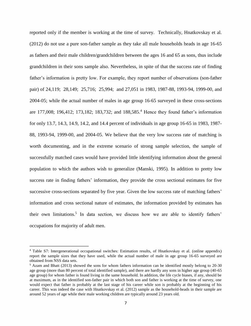
reported only if the member is working at the time of survey. Technically, Hnatkovskay et al.
(2012) do not use a pure son-father sample as they take all male households heads in age 16-65
as fathers and their male children/grandchildren between the ages 16 and 65 as sons, thus include
grandchildren in their sons sample also. Nevertheless, in spite of that the success rate of finding
father’s information is pretty low. For example, they report number of observations (son-father
pair) of 24,119; 28,149; 25,716; 25,994; and 27,051 in 1983, 1987-88, 1993-94, 1999-00, and
2004-05; while the actual number of males in age group 16-65 surveyed in these cross-sections
are 177,008; 196,412; 173,182; 183,732; and 188,585.4 Hence they found father’s information
for only 13.7, 14.3, 14.9, 14.2, and 14.4 percent of individuals in age group 16-65 in 1983, 1987-
88, 1993-94, 1999-00, and 2004-05. We believe that the very low success rate of matching is
worth documenting, and in the extreme scenario of strong sample selection, the sample of
successfully matched cases would have provided little identifying information about the general
population to which the authors wish to generalize (Manski, 1995). In addition to pretty low
success rate in finding fathers’ information, they provide the cross sectional estimates for five
successive cross-sections separated by five year. Given the low success rate of matching fathers’
information and cross sectional nature of estimates, the information provided by estimates has
their own limitations.5 In data section, we discuss how we are able to identify fathers’
occupations for majority of adult men.
4 Table S7: Intergenerational occupational switches: Estimation results, of Hnatkovskay et al. (online appendix)
report the sample sizes that they have used, while the actual number of male in age group 16-65 surveyed are
obtained from NSS data sets. 5 Azam and Bhatt (2013) showed the sons for whom fathers information can be identified mostly belong to 20-30
age group (more than 80 percent of total identified sample), and there are hardly any sons in higher age group (40-65
age group) for whom father is found living in the same household. In addition, the life cycle biases, if any, should be
at maximum, as in the identified son-father pair in which both son and father is working at the time of survey, one
would expect that father is probably at the last stage of his career while son is probably at the beginning of his
career. This was indeed the case with Hnatkovskay et al. (2012) sample as the household-heads in their sample are
around 52 years of age while their male working children are typically around 23 years old.

8
Motiram and Singh (2012) also use the IHDS data as used in our paper.6 In addition to
transition matrices, they present mobility measures 𝑀1: probability that a son (or the expected
proportion of sons) will leave the father’s occupational category and measures based on
eigenvalues of transition matrices for SC/STs and non-ST/STs, rural/urban, and age cohorts.7
They report a considerable intergenerational occupational persistence—across all occupational
categories, the father’s category is the most likely one that a son could find himself in (e.g. a
likelihood of almost half for agricultural laborers). But, there are differences across occupational
categories—the probability that a son would fall in the father’s category is higher for the low-
skilled/low-paying occupations. They also find that mobility is higher in urban areas as
compared to rural areas. Comparison of mobility for SC/STs and non-SC/STs gives ambiguous
results. However, they document considerable downward mobility for the SC/STs and show that
this is higher than the same for non-SC/STs. For SC/STs, they also observe higher persistence
(as compared to the same for non-SC/STs) in low-skilled/low-paying occupations.
Our study differs from Hnatkovskay et al. (2012) and Motiram and Singh (2012) in the
following ways. First, unlike Hnatkovskay et al. (2012), we are able to identify fathers’
occupations for majority of adult males, and provide occupation-specific human capital
transmission between fathers and sons spanning birth cohorts from 1945 to 1984. Second,
although similar to Hnatkovskay et al. and Motiram and Singh, we present the simple measure of
mobility (as measured by off-diagonal elements); however, we further distinguish between
6 Our sample is much larger than the sample used by Motiram and Singh (2012). As reported in appendix-1, Table
A1, our final sample consists of 38,294 son-father pairs. While our sample is restricted to males in age group 21-60,
Motiram and Singh restrict their sample to males in age group 20-65. In spite of a larger age band used, they report a
sample of 28,270 son-father pair (footnote of Table-1 of Motiran and Singh). As they have not provided details of
sample construction, we are unable to comment on their smaller sample. Our data appendix and appendix-1, Table
A1 provide our sample construction in detail. 7 They report 𝑀3 = 1 − |𝜆2| and 𝑀4 = 1 − | ∏ 𝜆𝑖|
𝑚=1 , where 𝜆2 is second largest eigenvalue of transition matrix
and 𝜆𝑖 are eigenvalues of transition matrix.

9
prevalence and associations. We estimate mobility measures after adjusting for differences in
occupation distributions. We think this is important as economy has been undergoing through
structural changes, and also corroborated by our findings (reported in results section) that after
adjusting for differences in occupation distributions, many of the conclusions based on simple
measure of mobility is changed. Moreover, following Ferrie (2005), Altham and Ferrie (2008),
and Long and Ferrie (2013), we estimate the Altham statistics, which provide a distance measure
between son-father occupation associations for two different cohorts/social groups. We also test
whether the difference in son-father occupation associations between two cohorts/groups is non-
zero. In addition, we further decompose the distance in associations to provide answers how
much and in which odds ratios, the son-father occupation association differ across birth
cohorts/groups.
2. Data
We use data from the India Human Development Survey, 2005 (IHDS), a nationally
representative survey of households jointly organized by the National Council of Applied
Economic Research (NCAER) and the University of Maryland. The IHDS covers 41,554
households in 1503 villages and 971 urban neighborhoods located throughout India.8 The survey
was conducted between November 2004 and October 2005 and collected a wealth of information
on education, caste membership, health, employment, marriage, fertility, and geographical
location of the household.
One of the major hindrances in carrying out any intergenerational study in developing
countries is lack of long panel data. In India, this problem is exacerbated as none of the large
8 The survey covered all the states and union territories of India except Andaman and Nicobar, and Lakshadweep.
These two account for less than .05 percent of India's population. The data is publicly available from the Data
Sharing for Demographic Research program of the Inter-university Consortium for Political and Social Research
(ICPSR).

10
cross sections (such as NSS or NFHS) collect information about father for all surveyed persons.
As noted in earlier discussion (section 1.1), the identification of father using the co-residence
lead to a sample which suffers from selection.9 In contrast to the NSS and the NFHS, the IHDS
data has asked specific questions regarding the education and occupation of household head's
father/husband (irrespective of the father/husband living in the household or not).10 In addition,
the IHDS also provides ID of father in the household roster which helps linking individuals to
their fathers directly if the father is living in the household. Combining these two variables, we
are able to identify fathers’ occupation for majority of male adults (21-60). A full description of
data construction is provided in appendix 1, Table1 and data appendix. There are certain
limitations of data for carrying out the task. First, optimally, one should have father and son’s
occupation at the same age. However, in our data, son’s occupation is the self-reported
occupation in the past year, while for majority of fathers; the occupation is the occupation for
most of father’s life as reported by son.11’12 Second, since we identify son’s occupation using the
self-reported occupation in the past year, it implies that we are using son’s occupation at
different points of their career based on their age.13 Although, the data is not the ideal for
carrying out an intergenerational occupational mobility task, it is a significant way forward given
9 Azam and Bhatt (2013) demonstrate that majority of adult males are household head themselves, and do not have
father living in the same households (or perhaps deceased), and this fact is also corroborated in appendix Table 1. 10 Question 1.19 and 1.20 on page 3 of the Household Questionnaire. 11 As noted earlier and shown in Appendix1, Table 1, majority (almost more than 60 percent) of men in age group
20-65 are household heads, and their fathers’ occupation is obtained from the question “What was the occupation of
the household head's father (for most of his life)?” For rest of the individuals who are not households heads, the
fathers occupation is based on observed occupation of father in the past year if the father is co-resident in the same
household. 12 One advantage of measuring intergenerational mobility by class or occupation is that the data restrictions are
much less stringent, retrospective information on father’s occupation is not difficult to collect and does not require
the investment in longitudinal data necessary for intergenerational income studies (Blanden, 2009). 13 Ex-ante, it is difficult to assess the life-cycle bias as there exists no nationally representative study on intra-
generational occupational mobility. However, the existing evidences based on case studies suggest that the life-cycle
bias may not be that strong. For example, Munshi and Rosenzweig (2009) document the lack of labor mobility in
India. Moreover, one may also think that occupation, broadly defined, varies less over the lifecycle making age–
related biases less problematic (Blanden, 2009).

11
the data constraints for such study in India. We have occupation information of fathers for
majority of adult male surveyed in nationally representative IHDS.14
Unlike income which is a continuous variable, the occupations are reported in two digits
occupation codes, and one need to aggregate the categories in few categories to get transition
matrices. The consensus on the classificatory schemes in the literature on mobility is lacking and
different authors have used different schemes, even when they have examined the same country
(e.g. Long and Ferrie 2005; Erikson and Goldthorpe 1992). We classify the occupation in four
groups: white collar workers, skilled/semi-skilled workers, unskilled workers (includes
agricultural wage workers), and farmers. Appendix 3 shows how we grouped the 2-digit
occupation codes to arrive at four groups. To examine the sensitivity of our findings with respect
to aggregation of occupations, we alternatively aggregated using the first digit of occupation
codes (in nine groups). We find qualitatively similar results with nine occupation groups.
3. Empirical Methodology
In this paper, we follow the methodology used in Long and Ferrie (2013, 2007), Altham and
Ferrie (2008), and Ferrie (2005), to compare the mobility across time and groups. Following the
literature on mobility, we first present the transition matrices, with categories for fathers’
occupations arrayed across one dimension and categories for sons’ occupations arrayed across
the other. However, comparing mobility across two time period or two social groups require
comparing two matrices. One simple measure of the overall mobility in matrix 𝑃 = [𝑝11 𝑝12
𝑝21 𝑝22],
14 As noted by Xie and Killwald (2013), we also do not wish to convey that data sources for measuring social
mobility in other countries/studies are flawless. We only wish to pinpoint some of the limitations of our data, and
how it is a significant improvement over the existing literature. Since an ideal data do not exist in the given context,
we have to rely on the existing data source and minimize the bias, which we claim to be doing by using a sample
which identify fathers information for majority of adult men in age group 20-65, and potentially reducing the life-
cycle bias, if there exists any, as we are using fathers’ occupation in which father spent most of his life time.
12
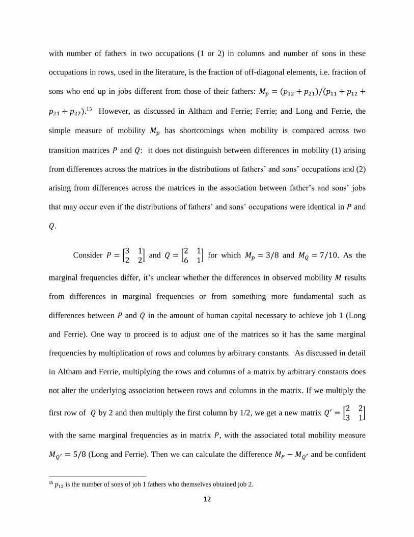
with number of fathers in two occupations (1 or 2) in columns and number of sons in these
occupations in rows, used in the literature, is the fraction of off-diagonal elements, i.e. fraction of
sons who end up in jobs different from those of their fathers: 𝑀𝑝 = (𝑝12 + 𝑝21)/(𝑝11 + 𝑝12 +
𝑝21 + 𝑝22).15 However, as discussed in Altham and Ferrie; Ferrie; and Long and Ferrie, the
simple measure of mobility 𝑀𝑝 has shortcomings when mobility is compared across two
transition matrices 𝑃 and 𝑄: it does not distinguish between differences in mobility (1) arising
from differences across the matrices in the distributions of fathers’ and sons’ occupations and (2)
arising from differences across the matrices in the association between father’s and sons’ jobs
that may occur even if the distributions of fathers’ and sons’ occupations were identical in 𝑃 and
𝑄.
Consider 𝑃 = [3 12 2
] and 𝑄 = [2 16 1
] for which 𝑀𝑝 = 3/8 and 𝑀𝑄 = 7/10. As the
marginal frequencies differ, it’s unclear whether the differences in observed mobility 𝑀 results
from differences in marginal frequencies or from something more fundamental such as
differences between 𝑃 and 𝑄 in the amount of human capital necessary to achieve job 1 (Long
and Ferrie). One way to proceed is to adjust one of the matrices so it has the same marginal
frequencies by multiplication of rows and columns by arbitrary constants. As discussed in detail
in Altham and Ferrie, multiplying the rows and columns of a matrix by arbitrary constants does
not alter the underlying association between rows and columns in the matrix. If we multiply the
first row of 𝑄 by 2 and then multiply the first column by 1/2, we get a new matrix 𝑄′ = [2 23 1
]
with the same marginal frequencies as in matrix 𝑃, with the associated total mobility measure
𝑀𝑄′ = 5/8 (Long and Ferrie). Then we can calculate the difference 𝑀𝑃 − 𝑀𝑄′ and be confident
15 𝑝12 is the number of sons of job 1 fathers who themselves obtained job 2.

13
that the difference in mobility does not result from differences in the distributions of occupations
between the two time periods or groups. This is still somewhat unsatisfactory as focusing on off-
diagonal elements but treating all moves identically discards a great deal of potentially useful
information (Long and Ferrie, 2007)
The fundamental measure of association between rows and columns in a mobility table is
the cross-product ratio, which for 𝑃 is 𝑝11𝑝22/𝑝12𝑝21 and can be rearranged to give (𝑝11
𝑝12 ) /
(𝑝21
𝑝22 ), the ratio of (1) the odds that sons of job 1 fathers get job 1 rather than job 2 to (2) the
odds that sons of job 2 fathers get job 1 rather than job 2. If there is perfect mobility, the cross-
product ratio would be one: sons of job 1 fathers would have no advantage in getting job 1
relative to sons of job 2 fathers. The more the cross-product ratio exceeds one, the greater the
relative advantage of having a job 1 father in getting job 1.
For a table with more than two rows or columns, there are several cross-products ratios.
Altham (1970) proposed a measure of the difference in relative mobility between two transition
matrices that is based solely on the odds ratios, and takes account of the full set of cross-products
ratios. For two tables 𝑃 and 𝑄 each have 𝑟 rows and 𝑠 columns, the Altham statistic 𝑑(𝑃, 𝑄):
𝑑(𝑃, 𝑄) = [∑ ∑ ∑ ∑ |𝑙𝑜𝑔 (𝑝𝑖𝑗𝑝𝑙𝑚𝑞𝑖𝑚𝑞𝑙𝑗
𝑝𝑖𝑚𝑝𝑙𝑗𝑞𝑖𝑗𝑞𝑙𝑚)
2
|
𝑠
𝑚=1
𝑟
𝑙=1
𝑠
𝑗=1
𝑟
𝑖=1
]
1/2
For two tables 𝑃 and 𝑄, the Altham statistic 𝑑(𝑃, 𝑄) measures the difference between 1)
the association between rows and columns in Table 𝑃 and 2) the association between rows and
14
columns in Table 𝑄.16 Replacing one table with a table of ones allows us to calculate 𝑑(𝑃, 𝐼) and
𝑑(𝑄, 𝐼), the distance between the association between rows and columns in Table 𝑃 or 𝑄 and the
association between rows and columns in a table in which rows and columns are independent.
These distance measures have likelihood ratio chi-square test statistics (𝐺2) to test the null
hypothesis that the associations do not differ, so one can assess whether two tables differ from
each other and from independence (Altham and Ferrie, 2007). If 𝑑(𝑃, 𝐼) < 𝑑(𝑄, 𝐼) and
𝑑(𝑃, 𝑄) ≠ 0, then Table 𝑃 has greater mobility than Table 𝑄 (that is, Table 𝑃 has an association
between rows and columns that is closer to what we would observe under independence than
does Table 𝑄).
The Altham statistic is a pure function of the odds ratios in each table, so it is not affected
by differences in the marginal frequencies (Ferrie, 2005). In addition, as [𝑑(𝑃, 𝑄)]2 is a simple
sum of the squares of log odds ratio contrasts, it can be decomposed into its constituent elements:
for an 𝑟 × 𝑠 table, there will be [𝑟(𝑟 – 1)/2][𝑠(𝑠 – 1)/2] odds ratios in 𝑑(𝑃, 𝑄) and it will be
possible to calculate how much each contributes to [𝑑(𝑃, 𝑄)]2, in the process identifying the
locations in 𝑃 and 𝑄 where the differences between them are greatest.
As contingency tables are often dominated by diagonal elements, we also calculate
another version of 𝑑(𝑃, 𝑄) that examines only the off-diagonal cells to see whether, conditional
on occupational mobility occurring between fathers and sons, the resulting patterns of mobility
are similar in 𝑃 and 𝑄. This new statistic will then test whether 𝑃 and 𝑄 differ in their proximity
to “quasi-independence.” (Agresti, 2002, p. 426) For square contingency tables with 𝑟 rows and
16 Altham and Ferrie (2007) discuss the distance measure and test statistic, and provide STATA algorithms for their
computation. In this paper, we have used the STATA algorithm provided in Altham and Ferrie.

15
𝑠 columns, this additional statistic 𝑑𝑖(𝑃, 𝑄) will have the same properties as 𝑑(𝑃, 𝑄), but the
likelihood ratio 𝜒2 statistic 𝐺2 will have [(𝑟 – 1)2 – 𝑟] degrees of freedom.
Similar to Long and Ferrie, Altham and Ferrie, and Ferrie, we also proceed in three steps:
First, we calculate total mobility for each table as the ratio of the sum of the off-diagonal
elements to the total number of observations in the table, and find the difference in total mobility
between 𝑃 and 𝑄;
Second, we adjust one of the tables to have the same marginal frequencies as the other and
recalculate the difference in total mobility to eliminate the influence of differences in the
distribution of occupations;
Third, we calculate 𝑑(𝑃, 𝑄), 𝑑𝑖(𝑃, 𝑄), 𝑑(𝑃, 𝐼), and 𝑑(𝑄, 𝐼) and the likelihood ratio 𝜒2 statistics
𝐺2; if 𝑑(𝑃, 𝑄) ≠ 0, we calculate the full set of log odds ratio contrasts and identify those making
the greatest contribution to [𝑑(𝑃, 𝑄)]2.
4. Results
4.1 Occupational mobility over time
Table 1 presents cross classification of son’s occupation by father’s occupation for son’s birth
cohorts 1945-1954 (panel 1), 1955-1964 (panel 2), 1965-74 (panel 3), and 1975-1984 (panel 4).
For the son’s birth cohort 1945-1954 (panel I, Table1), about 53.4 percentage of the sons born to
white collar occupation fathers end up in white color jobs. This percentage gradually declined in
later birth cohorts. For example, in birth cohort 1955-1964 (panel 2, Table 1), 43.0 percentage of
sons born to white collar occupation fathers end up in white collar jobs; in birth cohort 1965-
1974, 44.4 percentage of sons born to white color fathers end up in white collar jobs; and in most
recent cohort born in 1975-1984, only 39.3 percentage of sons born to white collar fathers end up

16
in white collar jobs. Thus, the persistence in transmission of white collar jobs from fathers to
sons has declined over time.
However, among sons of skilled/semi-skilled and unskilled occupation fathers, the
persistence in transmission of occupation to sons from fathers has increased. For example, the
62.7 percent of sons born during 1945-1954 to skilled/semi-skilled fathers ended up in the same
occupation, whereas about 71.9 percent of sons born during 1975-1984 to skilled/semi-skilled
fathers ended up in the same occupation. In addition, there is also less movement observed in
recent cohorts to white collar jobs of sons who were born to skilled/semi-skilled workers. For
example, 20.8 percent of sons born during 1945-54 to skilled/semi-skilled workers ended up in
white collar jobs, whereas this percentage declined to 17.1 percent in birth cohort 1955-1964, to
14.7 percentage in birth cohort 1965-1974, and 10.0 percentage in birth cohort 1975-1984.
The persistence of occupation also exists in sons born to fathers with unskilled jobs, and
this persistence has increased over time. Whereas the probability of someone born to unskilled
fathers getting a white collar job has been declining, the probability of someone born to unskilled
workers getting a skilled/semi-skilled job increased before experiencing a drop in the most recent
cohort.
Over time the importance of farming has been declining in Indian economy, and
movement into farming is increasingly seen not as a route to economic advancement. Only 43.9
percent of sons born during 1945-1954 to farmer fathers ended up working as farmer. This
probably suggests movement out of agriculture from a very predominant farming society. The
persistence of occupation to sons born to farmer fathers declined in sons born during 1945-1974,
however, the persistence seems to have increased in recent cohort, which seems a little bit

17
counterintuitive. However, the percentage of sons of farmers ending up with white collar or
skilled/semi-skilled jobs has declined in recent cohort after increasing during 1945-1975. In
addition, the percentage of sons of farmers ending up with unskilled jobs (includes agricultural
laborers) increased in birth cohort 1955-1964, before decreasing in 1965-1974, and in birth
cohort 1975-84. So, there is a possibility that sons born to farmer fathers in recent cohorts prefer
staying in same occupation than moving to unskilled category, whereas getting a white collar job
becoming more difficult for sons born to farmers. Sons of farmers born during 1975-1984 are
two-third as likely to get a white collar job as sons born during 1945-1954 to farmer fathers.
In Table 2, we present the summary measures of mobility. Table 2, panel 1, column 1
shows the simple measure of total mobility 𝑀, and according to this the cohort born in 1945-
1954 are more likely than the cohort born in 1955-1964 to find themselves in the occupations of
their fathers. The mobility is 3.0 percentage points higher in the sons’ cohort born during 1955-
64 compared with sons’ cohort born during 1945-54. However, the difference is mainly as a
result of differences in occupational distributions. If the total mobility is measured using 1955-64
birth cohort occupation distributions, it is the 1945-54 birth cohort who have a 0.6 percentage
points advantage in mobility compared with 1955-64 birth cohort (53.7 vs. 53.1), not the 1955-
64 cohort as suggested by simple measure of mobility. The earlier cohort, 1945-54, also shows a
higher mobility, by 0.9 percentage points using 1945-54 occupation distributions (50.1 vs. 49.2).
The Altham statistics for the 1945-1954 birth cohort (𝑃) and 1955-1964 birth cohort (𝑄)
are: 𝑑(𝑃, 𝐼) = 22.2, and 𝑑(𝑄, 𝐼) = 21.9, and both are significant at 1% significance level. Thus
we can reject the null hypothesis that the association between rows and columns was the same as
it would have under independence. In addition, these measures suggest that the association
between fathers’ and sons’ occupations was slightly closer to independence (that is, it exhibited

18
greater mobility) in the 1955-1964 birth cohort than in the 1945-1954 birth cohort, which is the
opposite of what we got when we measured mobility adjusting for occupation distributions (we
found marginal advantage for 1945-54 cohort). However, the difference between 𝑃 and 𝑄 in
their degree of association (panel 1, column 5, Table 2), 𝑑(𝑃, 𝑄), is small in magnitude (3.2), and
we cannot reject the null hypothesis that their associations are identical. Hence, we conclude that
that the occupational mobility in 1955-64 cohort is more or less similar to the mobility observed
in the 1945-1954 birth cohort. As we cannot reject the null of equal association in 𝑃 and 𝑄 when
we focus only on the off-diagonal elements (column 6, panel 1, Table 2), we conclude that the no
difference in mobility in two cohorts is not solely because of strong similarities in tendency of
sons to inherit their fathers occupations.
Table 2, panel 2 compares the mobility across birth cohort 1955-1964 (𝑃) and 1965-1974
(𝑄). The simple mobility measure suggests that the mobility was higher in birth cohort 1965-
1974 by 1.3 percentage points compared with the mobility observed in the birth cohort 1955-
1964. If mobility is measured for both cohorts using either the 1955-64 cohort (53.1 vs. 53.4) or
1965-1974 cohort’s (54.2 vs. 54.4) distributions of occupations, the advantage of 1965-74 cohort
is 0.2 percentage points to 1.3 percentage points. The Altham statistics for the 1955-1964 birth
cohort (𝑃) and 1965-1974 birth cohorts are: 𝑑(𝑃, 𝐼) = 21.9, and 𝑑(𝑃, 𝑄) = 21.0, and both are
significant at 1% significance level. These measures suggest that the association between fathers’
and sons’ occupations was closer to independence in the 1965-1974 birth cohort than in the
1955-1964 birth cohort. However, 𝑑(𝑃, 𝑄) = 3.7 is small, and we could not reject the null of
equality of association between the matrices. Hence, we conclude that occupational mobility in
1955-64 birth cohort is more or less similar to the mobility observed in the 1965-1974 birth
cohort.

19
Table 2, panel 3, compares the mobility across birth cohort 1965-74 (𝑃) and most recent
cohort 1975-1984 (𝑄). Simple measure of mobility suggests sharp decline in mobility between
1965-74 and 1975-84 birth cohorts: mobility declined by 7 percentage points. However, after
adjusting distributions of occupations, if total mobility is measured using the 1965-74 cohort
distribution of occupation, the observed decline in mobility falls from 7 percentage points to 0.7
percentage points (54.4 vs. 53.7) only. Similarly, if mobility is measured using 1975-84
occupation distribution, the gap in mobility falls from 7 percentage points to only 0.3 percentage
points (47.7 vs. 47.4). The Altham statistics for the 1965-1974 birth cohort (𝑃) and 1975-1984
birth cohorts are: 𝑑(𝑃, 𝐼) = 21.0, and 𝑑(𝑄, 𝐼) = 20.8, and both are significant at 1% significance
level. In addition, 𝑑(𝑃, 𝑄) = 4.6, and it’s significant at 1% significance level. However, since
𝑑(𝑃, 𝐼) ≈ 𝑑(𝑄, 𝐼), and 𝑑(𝑃, 𝑄) > 0, tables 𝑃 and 𝑄 have row-column associations that are
equally distant from the row-column association observed under independence, but tables 𝑃 and
𝑄 differ in how they differ from independence, i.e. the odds ratios in table 𝑃 that depart the most
from independence are different from those that depart the most from independence in table 𝑄.
Overall, there is no strong evidence in differences in mobility in successive ten year birth
cohorts except between the 1965-74 and 1975-84 birth cohorts. However, the difference in 1965-
74 and 1975-84 contingency tables are that they differ in how they differ from independence.
Looking at longer period gap (panel 4, Table 2), between cohorts 1945-54 (𝑃) and 1975-84 (𝑄),
the simple measure of mobility suggests a decline in mobility by 2.7 percentage points. After
adjusting for occupational differences, the mobility in the recent cohort is just 0.5 percentage
points less (using 1945-54 occupation frequencies, 47.9 vs. 47.4 or using 1975-84 occupation
frequencies, 50.1 vs. 49.6). Finally, if the two birth cohorts had swapped the occupational
distributions and retained their underlying associations between fathers’ and sons’ occupations,

20
the recent birth cohort (1975-1984) shows an advantage in mobility by 1.7 percentage points.
Importantly, 𝑑(𝑄, 𝐼) < 𝑑(𝑃, 𝐼), and 𝑑(𝑃, 𝑄) ≠ 0, the Altham Statistics suggest that the mobility
in recent cohort is higher than the mobility in the 1945-54 birth cohort. Moreover, as we can
reject the null of equal association even when the diagonal elements in 𝑃 and 𝑄 are excluded,
this suggests the difference is not driven by change in the likelihood of direct inheritance of the
father’s occupational status, but there are change in structure of association between two
generations occupations.
As, we aggregated the 2-digit occupation categories into four groups which are much
broader, it is important to know how our conclusions differs if we define occupation groups more
finely. For this, we divided the occupations into nine groups based on 1-digit Indian National
Classification of Occupations (NCO) classification.17 To preserve the space, we only provide the
calculated summary measures in appendix Table A2, and do not report the transition tables. The
magnitudes of the Altham statistics increased substantially for all cohorts; however, we cannot
reject null of equal association between birth cohorts 1945-54 (𝑃) and 1955-64 (𝑄), and
between birth cohorts 1955-64 (𝑃) and 1965-74 (𝑄). This is similar to what we found with four
occupation categories. For birth cohorts 1965-74 (𝑃) and 1975-84 (𝑄), we find that although
𝑑(𝑃, 𝑄) > 0, but 𝑑(𝑃, 𝐼) ≈ 𝑑(𝑄, 𝐼). Qualitatively this result is similar to results with four
occupation categories: tables P and Q have row-column associations that are equally distant from
the row-column association observed under independence, but tables 𝑃 and 𝑄 differ in how they
differ from independence. Looking at longer gap, for birth cohort 1945-54 (𝑃) and 1975-84 (𝑄),
we find 𝑑(𝑃, 𝐼) = 110.2 > 𝑑(𝑄, 𝐼) = 98.8, and 𝑑(𝑃, 𝑄) > 0, hence the mobility seems higher in
the recent cohort. Thus the findings with nine occupation categories are broadly consistent with
17 The NCO is based upon the International Labour Organization (ILO) ISCO classification, suitably modified for
the Indian conditions

21
the findings with the four occupation categories, and we continue the rest of the analysis using
the four occupation categories.
Table 3 presents the components which has contributed at least 5 percentage points in
the difference between association in 𝑃 (1945-54 birth cohort) and 𝑄 (1975-84 birth cohort).18
These components account for more than 90 percent of difference between associations. The first
entry is the relative advantage in entering farming rather than unskilled work from having a
skilled father rather than unskilled father. In recent cohort, 1975-84 birth cohort, sons of skilled
fathers are 5.6 times more likely to enter farming rather than unskilled work than were the sons
of unskilled fathers. In the 1945-54 cohort, the ratio was only 1.6 to one. Hence advantage of
having a skilled father rather than unskilled father in making a move into farming rather than
unskilled work is 3.5 times greater in 1975-84 cohort than in 1945-54 cohort. This odd ratio
contrast account for 11.5 percent of the difference in association between 𝑃 and 𝑄. The second
entry also contributes 11.4 percent of the difference in association between 𝑃 and 𝑄. It shows the
relative advantage in entering farming rather than unskilled work from having a white collar
father rather than an unskilled father. The odds ratio suggests that the relative advantage
increased 2.9 times to 10.3 times between the two cohorts for such a move (moving to farming
rather than to unskilled work) for sons with white collar father than sons with unskilled father.
There seems also a decline in the disadvantage in entering white collar job rather than other jobs
for sons of non-white collar fathers. For example, the third entry in Table 3 shows that the
relative advantage in entering in white collar job rather than farming from having a skilled job
father rather than having a unskilled job father declined from six times to two times. Similarly,
the tenth entry in Table 3 shows that the relative advantage in entering in white collar job rather
18 We do not carry out the decomposition analysis for successive birth cohorts as the difference in association
between sons and fathers’ occupations between successive birth cohorts are not statistically significant.
22
than farming from having a white collar father rather than having a unskilled job father declined
from 11.6 times to 4.6 times. The 12th entry shows that the relative advantage in entering in
white collar job rather than farming from having a white collar father rather than having a farmer
father declined from 45.3 times to 19.1 times.
4.2 Occupational mobility among different social groups
Although there exists many studies on Indian caste system, only few has tried to address
intergenerational mobility issues. To answer the question of whether mobility differs across
social groups, we re-ran our analysis for different social groups. However, to boost the cell size,
this analysis is based of 20 year birth cohort rather than 10 year birth cohort. Table 4 provides
cross classification of son’s occupation by father’s occupation for son’s born during 1945-64 and
1965-84 for different social groups. Table 5 presents the summary measures of mobility. Based
on simple measure of mobility (column (1) of Table 5), mobility among higher castes sons born
during 1965-84 has been lower by 0.8 percentage points when compared with mobility among
higher castes sons born during 1945-64. However, if we calculate mobility in both higher castes
birth cohorts based on 1965-84 occupation distributions, mobility is marginally higher in the
1965-84 cohort (51.6 vs. 51.7). Similarly, based on the 1945-64 higher castes birth cohort’s
occupation distributions, the mobility in 1965-84 higher castes birth cohort is marginally higher.
Moreover, the more fundamental measure of mobility, the Altham statistics, suggests that the
1965-84 higher castes birth cohort is closer to independence than the 1945-64 higher castes birth
cohort. Also we can safely reject the null of equal association between the two higher castes
cohorts. Since, 𝑑(𝑃, 𝑄) > 0 and 𝑑(𝑃, 𝐼) > 𝑑(𝑄, 𝐼), we conclude the mobility is higher among the
recent cohort for higher castes.
23
For Scheduled Castes/Tribes, the simple measure of mobility suggests a decline in
mobility in recent cohort (column 1, panel 2, Table 5) by 0.8 percentage points. However, once
we take account of differences in occupation distributions, the recent cohort among SC/STs has
about 2 percentage point advantage over the sons born during 1945-64 to SC/STs fathers. The
Altham statistics also suggests that the row-column association is closer to independence among
1965-84 cohort than among the 1945-64 cohort. We also can reject the null of identical
association among these two cohorts. As 𝑑(𝑃, 𝑄) > 0, and 𝑑(𝑄, 𝐼) < 𝑑(𝑃, 𝐼), we conclude that
the mobility among the recent SC/STs cohort is higher. More importantly, even we remove the
diagonal elements, association off the diagonal elements differ across the two cohorts.
For OBCs, the simple measure again suggests a lower mobility (1.3 percentage points
less) in recent cohort (panel 3, Table 5). Adjusting for occupation distribution reduces the gap in
mobility; however, the recent cohort still has marginally less mobility. The Altham Statistics
suggests 𝑑(𝑃, 𝑄) > 0, and 𝑑(𝑃, 𝐼) ≈ 𝑑(𝑄, 𝐼), which implies that tables (cohort 1945-64) 𝑃 and
𝑄 (cohort 1965-84) have row-column associations that are equally distant from the row-column
association observed under independence, but tables 𝑃 and 𝑄 differ in how they differ from
independence.
For Muslims, the simple measure suggests a lower mobility among recent cohort (panel
4, Table 5). Adjustments in occupation distributions reduce the disadvantage of recent cohort
from about 2 percentage point to less than 1 percentage point. However, the Altham Statistics
suggests that the row-column association in recent cohort is closer to independence than the row-
column association in birth cohort 1945-64. Nevertheless, we fail to reject identical associations
in two cohorts, and conclude no changes in mobility.
24
To summarize, the mobility in recent birth cohort (1965-84) has been higher (compared
with the birth cohort 1945-64) for higher castes and SC/STs, whereas for Muslims, the mobility
is not statistically different among the two cohorts.
Table 6 reports the components which have made at least 5 percent contribution in
[𝑑(𝑃, 𝑄)]2. For higher castes, the two largest contributors in difference in son-father’s
occupation association between the birth cohort 1945-64 and 1965-84 suggest that relative
advantage in entering farming rather than unskilled jobs from having a white collar/skilled father
rather than having an unskilled job father increased in recent cohort. This is similar to the overall
population story presented in the last section. For SCs/STs, the two important contributors
suggest decline in advantage in entering white collar job rather than farming from having a white
collar father rather than a farmer father; and increase in odds of getting white collar job rather
than farming from having a farmer father rather than having a skilled job father. This suggests
that the chance of upward mobility in recent SC/ST cohort is higher than the earliest cohort. In
contrast, for OBCs, the relative advantage in entering white collar jobs rather than non-white
collar jobs from having a white collar father rather than non-white collar father increased in
recent cohort (entry 5, 7, 8 in the panel 3, Table 6).
4.3 Does the mobility differ across social groups?
The differences among social groups remain an important issue in India. We compare the
differences among social groups in two ways. First, we compare mobility among each social
group to total population mobility. Second, we compare mobility in different social groups to
mobility among higher castes. Table 7 reports comparisons of mobility among each social group
to mobility among entire population for two birth cohorts 1945-64 (panel I of Table 7) and 1965-
84 (panel II of Table 7). For birth cohort 1945-64, although the simple measure of mobility

25
suggests marginally higher (lower) mobility among higher castes and OBCs (SC/ST and
Muslims) compared with the mobility in the entire population, we fail to reject the null of
identical association among each group and population at conventional (5 percent) significance
level. Hence for the birth cohort 1945-64, we find no evidence of difference in association
between father and son’s occupation in each social group to the association observed in the entire
population.
Next we compare mobility for individuals born during 1965-84. The simple measure of
mobility suggests that the mobility has been higher among higher castes compared to entire
population by 0.9 percentage points (row 1, panel B, Table 7). After adjusting for differences in
occupation distributions, the mobility advantage for higher castes remains (about 1 percentage
points). As, 𝑑(𝑃, 𝐼) < 𝑑(𝑄, 𝐼), and 𝑑(𝑃, 𝑄) > 0, the Altham statistics suggest that in birth cohort
1965-84, the mobility is higher among higher castes compared with mobility among entire
population. Simple measure of mobility also suggests marginally higher mobility among SC/STs
(0.2 percentage points) compared to the all in birth cohort 1965-84. The gap becomes larger after
adjusting for occupational distributions. The SC/ST advantage increase to 2.3 percentage points
if mobility is measured using the population occupation distribution (51.0 vs. 48.8), while the
advantage is 2.6 percentage points using the SC/ST occupation distribution (53.4 vs. 50.8). The
Altham Statistics also confirms a higher mobility among SC/STs compared to the entire
population born during 1965-84.
For OBCs, the simple mobility measure shows 0.4 percentage points advantage in 1965-
84 birth cohort (row 3, panel II, Table 7). Adjusting for occupation does not affect the gap.
However, we fail to reject the null of equality of mobility among OBCs and entire population for

26
birth cohort 1965-84. Hence, we conclude the mobility among OBCs born during 1965-84 is not
very different from the mobility experienced by all who were born during 1965-84.
Similarly, the simple measure of mobility suggests a 3.7 percentage point disadvantage
for Muslims born during 1965-84 compared to all who were born during the same period.
However, after adjusting for occupational distributions the disadvantage in mobility turn out to
be much smaller (less than 1 percentage point). Moreover, we fail to reject the null of equality of
row-column associations in Muslims and all population at conventional level of significance.
Overall, for the birth cohort 1945-64, we do not find any evidence of difference in
mobility among any social group when compared with the entire population; however, for the
birth cohort 1965-84, we find higher mobility among higher castes and SC/STs than the mobility
in entire population.
One may also be concerned about the difference between the disadvantaged social groups
and the higher castes. To get these differences, we compare each social group with the higher
castes. Table 8 provides comparisons of mobility among each social group to mobility among
higher castes. For birth cohort 1945-64 (panel 1 of Table 8), we fail to reject the null of identical
associations between OBCs or Muslims and higher castes. However, we can safely reject
identical association among SC/STs and higher castes. The simple measure of mobility suggest
0.7 percentage point disadvantage for SC/STs when compared with the higher castes. This
disadvantage increases once we adjust for occupations (50.7 vs. 52.5 or 51.8 vs. 52.5). As
𝑑(𝑃, 𝐼) > 𝑑(𝑄, 𝐼), and 𝑑(𝑃, 𝑄) > 0, the association between fathers and sons occupation
differed from independence more among SC/STs than among the higher castes. Hence, we

27
conclude that the mobility among SC/STs was lower than mobility among higher castes in birth
cohort 1945-64.
For birth cohort 1965-84 (panel 2, Table 8), the simple measure of mobility suggests that
the mobility among SC/STs is lower than mobility among higher castes by 0.7 percentage points.
However, the disadvantage of SC/STs turns out to be advantage from 1.2 (51.0 vs. 49.8) to 1.7
(53.4 vs. 51.7) percentage points after adjustment of occupational distributions. The more
fundamental measure of association 𝑑(𝑃, 𝐼) and 𝑑(𝑄, 𝐼) also shows a weaker association (more
mobility) among SC/STs compared with the higher castes. As 𝑑(𝑃, 𝑄) > 0, and 𝑑(𝑃, 𝐼) <
𝑑(𝑄, 𝐼), we conclude that the mobility among SC/STs is higher than the mobility among higher
castes in birth cohort 1965-84. However, we fail to reject the equality of association between
Muslims and higher castes at conventional level of significance. The simple measure of mobility
suggest slight disadvantage for OBCs compared to higher castes. The slight disadvantage for
OBCs persists even after adjusting for occupation distributions. Moreover, we reject the null of
equality of association between OBCs and higher castes. As 𝑑(𝑃, 𝑄) > 0, and 𝑑(𝑃, 𝐼) ≈ 𝑑(𝑄, 𝐼),
we conclude the OBCs and higher castes have row-column associations that are equally distant
from the row-column association observed under independence, but associations among OBCs
and higher castes differ in how they differ from independence.
Table 9 reports the components which have largest contribution in difference in
association between SC/STs and higher castes. Panel 1 of Table 9 reports this for 1945-64 birth
cohort. The first two entries contribute almost 23 percent of the differences. The first entry is
relative advantage of entering into white collar job than farming from having a white collar
father than a skilled occupation father. The relative advantage is 2.6 times among SC/STs while
it is only 0.9 times among higher castes. The second entry is relative advantage of entering into

28
white collar job than unskilled job from having a white collar father than an unskilled father. The
relative advantage is 38.4 times among SC/STs compared with 15.4 times among higher castes.
Of the thirteen odd ratios that account for more than 75 percent of difference among SC/STs and
higher castes, eight displays a higher advantage in entering white collar job for sons of white
collar fathers among SC/STs than among higher castes.
For birth cohort 1965-84 (panel 2, Table 9), the highest contributor to the difference
between SC/STs and higher castes suggest that the odds of entering in white collar job rather
than farming from having a farmer father than skilled occupation father is two times higher
among SC/STs when compared with the higher castes. Similarly, the third entry suggest that
relative advantage in entering white collar job rather than unskilled job from having skilled job
father rather than having an unskilled father is less in SC/STs than higher castes (1.5 times vs.
4.2 times).
The difference in mobility based on geographical dimensions, such as urban/rural or
states remains an important question. However, we only know the area of residence at the time of
survey, and due to urbanization (or migration) over time more areas might have been classified
as urban making it difficult to compare mobility across cohorts by urban/rural residence. In
addition, we do not have enough sample sizes to do our analysis over time by states. Hence, we
do not attempt to examine differences in mobility across geographical dimensions.
5. Conclusion
In this paper, we address the issue of occupation-specific human capital transmission
between fathers and sons in India spanning birth cohorts from 1945 to 1984. We are able to find
fathers’ occupation information for majority of adult males surveyed in the nationally

29
representative India Human Development Survey (IHDS). In addition, we also examine the
differential in mobility across social groups.
We find that the simple measure of mobility (fraction of sons who end up in jobs
different from those of their fathers) provide an incomplete picture in changing economy. Many
of the findings based on simple measure of mobility are reversed once we adjust for differences
in marginal distributions of occupations to disentangle the true association between father-son
occupations. Using the Altham statistics which provides a more robust measure of distance
(Long and Ferrie, 2013, 2007; Altham and Ferrie, 2008; and Ferrie, 2005) between the
associations of son-father occupations across cohorts/groups, we find no strong evidence in
differences in mobility in successive ten year birth cohorts except between the 1965-74 and
1975-84 birth cohorts. Moreover, the 1965-74 and 1975-84 birth cohorts differ in how they differ
from independence, i.e. the odds ratios---for example, the odds that the son of a white collar
father would get a white collar job compared with the odds that the son of a low-skilled father
would get a white collar job---in the birth cohort 1965-74 that depart the most from
independence (odds ratio of one) are different from those that depart the most from independence
in the birth cohort 1975-84. Interesting, these two birth cohorts are likely to have entered in labor
market in the late 1980s and 1990s, which saw a dramatic shift in Indian economic policy from a
closed economy to increasingly globalized economy following the liberalization introduced in
May, 1991. In this paper, we haven’t tried to assess the importance of the shift in the economic
policy in affecting the intergenerational occupation mobility; however, we believe that this
remains an important direction of future work.
We also find that the mobility among higher castes and SC/STs has been higher in birth
cohort 1965-84 when compared with the 1945-64 birth cohort. Moreover, although SC/STs had a

30
lower mobility compared with higher castes in birth cohort 1945-64; they experienced a higher
mobility compared with the higher castes in the 1965-84 birth cohort. SC/STs have been
beneficiaries of the affirmative action policy under which a quota of places, in higher education
and in government jobs, has been reserved for them. If the caste system (as it is widely believed)
trapped many potentially talented people at the lower levels of the society, then the affirmative
policy potentially could lead to a period of social mobility among SC/STs. Although we
document improvement in mobility in SC/STs over time and compared with the higher castes,
we do not attempt to assess whether the improvement in mobility among SC/STs are a result of
the affirmative policy. However, we believe that our work will provide foundations for any
future work in these directions.
31
References
Agresti, A (2002), Categorical Data Analysis, New York: Wiley-Interscience.
Altham, P.M.E and Ferrie, J.P. (2007), Comparing Contingency Tables: Tools for Analyzing
Data from Two Groups Cross-Classified by two Characteristics, Historical Methods, 40(1), 3-16.
Azam, M and Bhatt, V. (2012), Like Father, Like Son? Intergenerational Educational Mobility
in India, IZA Discussion Paper, 6549.
Black, S. E and Devereux, P. J. (2010),Recent developments in intergenerational mobility,
National Bureau of Economic Research Working Paper Series, No. 15889.
Blanden, J. (2009), How Much Can We Learn From International Comparisons Of
Intergenerational Mobility?, Centre for the Economics of Education DP, 111, London School of
Economics.
Björklund, A and Jäntti, M. (2000), Intergenerational mobility of socio-economic status in
comparative perspective, Nordic Journal of Political Economy, 26, 3-33.
Bourdieu, J., Ferrie, J., and Kesztenbaum, L. (2006), Vive la différence? Intergenerational
Occupational Mobility in France and the U.S. in the 19th and 20th Centuries, available at
http://mauricio.econ.ubc.ca/pdfs/ferrie.pdf
Breen, R. (2004), Social Mobility in Europe, Oxford University Press.
Desai, S. B., Dubey, A., Joshi, B. L., Sen, M., Shariff, A., and Vanneman, R. ( 2010), Human
Development in India: Challenges for a Society in Transition, Oxford University Press.
Despande, A. (2000), Does Caste Still Define Disparity? A Look at Inequality in Kerala, India,
American Economic Review Papers and Proceedings, 90(2), 322-25.
DiPrete, T. A. and Grusky, D.B. (1990), Structure and Trend in the Process of Stratification for
American Men and Women, American Journal of Sociology, 96(1), 107-43.
Erikson, R. & Goldthorpe, J. H. (1992), The Constant Flux – A Study of Class Mobility in
Industrial Societies, Clarendon, Oxford, England.
Ferrie, J.P. (2005), History Lessons: The End of American Exceptionalism? Mobility in the
United States Since 1850, Journal of Economic Perspectives, 19( 3), 199–215.
Ganzeboom, H. B. G. and Treiman, D. J. (1996), Internationally Comparable Measures of
Occupational Status for the 1988 International Standard Classification of Occupations, Social
Science Research, 25 (2): 201-39.

32
Hellerstein, J.K and and Morrill, M.S. (2011), Dads and Daughters: The Changing Impact of
Fathers on Women’s Occupational Choices, Journal of Human Resources, ,46, 333-372.
Hnatkovskay, V., Lahiri, A. and Paul S.B. (2013), Breaking the Caste Barrier:
Intergenerational Mobility in India, Journal of Human Resources, 48(2), 435-73.
Jäntti, M., Bratsberg, .B., Røed, K., Raaum, O., Naylor, R., Österbacka, E., Björklund, A.
and Eriksson, T. (2006). American Exceptionalism in a New Light: A Comparison of
Intergenerational Earnings Mobility in the Nordic countries, the United Kingdom and the United
States, IZA Discussion Paper, 1938.
Long, J and Ferrie, J. (2013), Intergenerational Occupational Mobility in Britain and the U.S.
Since 1850, American Economic Review, 103(4): 1109-37.
Long, J and Ferrie, J. (2007), The Path to Convergence: Intergenerational Occupational
Mobilty in Britain and the US in Three Eras, Economic Journal, C61-C71.
Maasoumi, E. (1997), On mobility, In: Giles, D. and Ullah,A. (Eds.), The Handbook of
Economic Statistics, Marcel Dekker, New York.
Majumder, R. (2010). Intergenerational Mobility in Educational and Occupational Attainment:
A Comparative Study of Social Classes in India, Margin-The Journal of Applied Economic
Research, 4 (4): 463-494.
Manski, C. (1995), Identification Problems in the Social Sciences, Cambridge, MA: Harvard
University Press
Motoram, S and Singh, A. (2012), How Close Does the Apple Fall to the Tree? Some Evidence
on Intergenerational Occupational Mobility from India, Economic and Political Weekly, Vol -
XLVII No. 40.
Munshi, K. and Rosenzweig, M. (2009), Why is Mobility in India so Low? Social Insurance,
Inequality, and Growth?, NBER Working Paper, 14850
Xie, Y.and Killewald, A. (2013), Intergenerational Occupational Mobility in Britain and the US
since 1850: Comment, forthcoming in American Economic Review.

33
Table 1: Intergenerational Occupational Mobility in India, 1945-1984 birth cohorts
Panel 1: Son's Birth Cohort=1945-1954
Panel 3: Son's Birth Cohort=1965-1974
Father's Occupation
Father's Occupation
Son's occupation White Collar
Skilled/Semi-skilled
Unskilled Farmers Row Sum
Son's occupation
White collar
Skilled/Semi-skilled
Unskilled Farmers Row Sum
White Collar 132 220 129 278 759
White Collar 294 361 224 500 1,379
(53.4) (20.8) (8.9) (9.1) (13.1)
(44.4) (14.7) (7.2) (9.8) (12.1)
Skilled/Semi-Skilled 78 663 394 660 1,795
Skilled/Semi-Skilled 264 1,758 1,008 1,588 4,618
(31.6) (62.7) (27.3) (21.7) (31.0)
(39.9) (71.6) (32.5) (30.9) (40.7)
Unskilled 23 131 764 773 1,691
Unskilled 66 278 1,711 1,639 3,694
(9.3) (12.4) (52.8) (25.3) (29.1)
(10.0) (11.3) (55.2) (31.9) (32.5)
Farmers 14 43 159 1,337 1,553
Farmers 38 59 155 1,414 1,666
(5.7) (4.1) (11.0) (43.9) (26.8)
(5.8) (2.4) (5.0) (27.5) (14.7)
Column sum 247 1,057 1,446 3,048 5,798
Column sum 662 2,456 3,098 5,141 11,357
Panel 2: Son's Birth Cohort=1955-1964
Panel 4: Son's Birth Cohort=1975-1984
Father's Occupation Father's Occupation
Son's occupation White collar
Skilled/Semi-skilled
Unskilled Farmers Row Sum
Son's occupation
White collar
Skilled/Semi-skilled
Unskilled Farmers Row Sum
White Collar 198 313 226 409 1,146
White Collar 307 301 175 299 1,082
(43.0) (17.1) (9.1) (9.4) (12.6)
(39.3) (10.0) (4.9) (6.4) (9.0)
Skilled/Semi-Skilled 190 1,286 764 1,180 3,420
Skilled/Semi-Skilled 302 2,167 1,059 1,326 4,854
(41.2) (70.2) (30.8) (27.3) (37.6)
(38.7) (71.9) (29.6) (28.4) (40.3)
Unskilled 51 195 1,347 1,307 2,900
Unskilled 77 328 2,089 1,273 3,767
(11.1) (10.7) (54.3) (30.2) (31.9)
(9.9) (10.9) (58.5) (27.3) (31.3)
Farmers 22 37 144 1,435 1,638
Farmers 95 219 250 1,766 2,330
(4.8) (2.0) (5.8) (33.1) (18.0)
(12.2) (7.3) (7.0) (37.9) (19.4)
Column sum 461 1,831 2,481 4,331 9,104
Column sum 781 3,015 3,573 4,664 12,033
Note: the numbers in parenthesis are percentage of column sum.

34
Table 2: Summary Measures of Mobility
M M' d(P, I) d(Q,I) d(P, Q) di(P, Q)
(1) (2) (3) (4) (5) (6)
1. Cohort 1945-1954 (P) 50.1 53.7 22.2***
3.2 1.7
vs. Cohort 1955-1964 (Q) 53.1 49.2
21.9***
2. Cohort 1955-1964 (P) 53.1 54.2 21.9***
3.7 2.0
vs. Cohort 1965-1974 (Q) 54.4 53.4
21.0***
3. Cohort 1965-1974 (P) 54.4 47.7 21.0***
4.6*** 3.3**
vs. Cohort 1975-1984 (Q) 47.4 53.7
20.8***
4. Cohort 1945-1954 (P) 50.1 47.9 22.2***
7.5*** 5.8***
vs. Cohort 1975-1984 (Q) 47.4 49.6
20.8***
Note: M is total mobility (percent off the main diagonal), M’ is total mobility using the marginal frequencies from the
Q matrix. Significance levels for the likelihood ratio 𝜒2 statistic 𝐺2 (d.f. 9 for d(P,I), d(Q,I), and d(P,Q); 5 for di(P,Q)):
*** < 0.01 ** < 0.05 * < 0.10.

35
Table 3: Components of d(P,I), d(Q,I), and d(P,Q) for sons’ birth cohort 1945-54 (P) vs. birth cohort 1975-84 (Q)
Contrast d(P,I) Odds
ratio d(Q,I) Odds
ratio d(P,Q) Percentage
of total Cumulative percentage
1. [(SF)/(SU)]/[(UF)/(UU)] 0.91*** 1.58 3.4*** 5.58 2.53*** 11.47 11.47
2. [(WF)/(WU)]/[(UF)/(UU)] 2.15*** 2.92 4.7*** 10.31 2.52*** 11.41 22.88
3. [(SW)/(SF)]/[(UW)/(UF)] 3.68*** 6.31 1.3*** 1.96 2.33*** 9.79 32.67
4. [(FW)/(FF)]/[(SW)/(SF)] 6.41*** 0.04 4.2*** 0.12 2.22*** 8.84 41.51
5. [(WF)/(WS)]/[(UF)/(US)] 1.62*** 0.44 0.6*** 1.33 2.19*** 8.65 50.16
6. [(WF)/(WS)]/[(FF)/(FS)] 4.85*** 0.09 2.9*** 0.24 1.96*** 6.91 57.07
7. [(SF)/(SS)]/[(UF)/(US)] 3.66*** 0.16 1.7*** 0.43 1.96*** 6.90 63.97
8. [(FF)/(FU)]/[(SF)/(SU)] 3.32*** 5.27 1.5*** 2.08 1.86*** 6.23 70.20
9. [(WF)/(WU)]/[(FF)/(FU)] 2.09*** 0.35 0.2 0.89 1.85*** 6.18 76.38
10. [(WW)/(WF)]/[(UW)/(UF)] 4.91*** 11.62 3.1*** 4.62 1.85*** 6.13 82.50
11. [(WW)/(WF)]/[(FW)/(FF)] 7.63*** 45.35 5.9*** 19.09 1.73*** 5.38 87.88
12. [(FF)/(FS)]/[(SF)/(SS)] 6.88*** 31.23 5.2*** 13.18 1.73*** 5.35 93.24
Notes: First element of each pair is father’s occupation, second is son’s. W: White Collar, S: Skilled/Semi-skilled, U: Unskilled, F: Farmer. Significance levels for the likelihood ratio 𝜒2 statistic 𝐺2. *** < 0.01 ** < 0.05 * < 0.10.

36
Table 4: Transition matrices for social groups
Panel 1: Higher castes
Panel 2: Other Backward Castes
Son's Birth Cohort=1945-1964
Son's Birth Cohort=1945-1964
White Collar
Skilled/semi-skilled
Unskilled Farmers Row sum
White Collar
Skilled/semi-skilled
Unskilled Farmers Row sum
White Collar 201 223 114 282 820
White Collar 57 150 115 245 567
(51.9) (23.2) (15.7) (13.3) (19.5)
(34.3) (17.0) (9.2) (8.4) (10.9)
Skilled/Semi-Skilled 138 647 267 542 1,594
Skilled/Semi-Skilled 73 595 389 666 1,723
(35.7) (67.2) (36.7) (25.5) (37.9)
(44.0) (67.2) (31.1) (22.8) (33.0)
Unskilled 29 73 254 405 761
Unskilled 24 109 637 817 1,587
(7.5) (7.6) (34.9) (19.1) (18.1)
(14.5) (12.3) (51.0) (28.0) (30.4)
Farmers 19 20 93 895 1,027
Farmers 12 31 109 1,195 1,347
(4.9) (2.1) (12.8) (42.1) (24.4)
(7.2) (3.5) (8.7) (40.9) (25.8)
Column sum 387 963 728 2,124 4,202
Column sum 166 885 1,250 2,923 5,224
Son's Birth Cohort=1965-1984
Son's Birth Cohort=1965-1984
White Collar
Skilled/semi-skilled
Unskilled Farmers Row sum
White Collar
Skilled/semi-skilled
Unskilled Farmers Row sum
White Collar 274 263 116 301 954
White Collar 173 203 128 280 784
(45.7) (18.2) (11.1) (11.1) (16.4)
(40.7) (11.7) (6.2) (7.1) (9.6)
Skilled/Semi-Skilled 234 1,007 370 804 2,415
Skilled/Semi-Skilled 158 1,235 621 1,108 3,122
(39.0) (69.7) (35.4) (29.5) (41.5)
(37.2) (70.9) (30.2) (28.2) (38.3)
Unskilled 37 113 442 535 1,127
Unskilled 51 187 1,150 1,120 2,508
(6.2) (7.8) (42.3) (19.6) (19.4)
(12.0) (10.7) (55.9) (28.5) (30.8)
Farmers 55 62 116 1,085 1,318
Farmers 43 116 157 1,418 1,734
(9.2) (4.3) (11.1) (39.8) (22.7)
(10.1) (6.7) (7.6) (36.1) (21.3)
Column sum 600 1,445 1,044 2,725 5,814
Total 425 1,741 2,056 3,926 8,148
Note: the numbers in parenthesis are percentage of column sum.

37
Table 4 (cont’d): Transition matrices for social groups
Panel 3: Scheduled Castes/Scheduled Tribes
Panel 4: Muslims Son's Birth Cohort=1945-1964
Son's Birth Cohort=1945-1964
White Collar
Skilled/ semi-skilled
Unskilled Farmers Row sum
White Collar
Skilled/ semi-skilled
Unskilled Farmers Row sum
White Collar 47 77 80 116 320
White Collar 25 83 46 44 198
(46.1) (14.0) (5.1) (6.5) (8.0)
(47.2) (16.9) (11.8) (7.9) (13.3)
Skilled/Semi-Skilled 36 358 357 473 1,224
Skilled/Semi-Skilled 21 349 145 159 674
(35.3) (65.2) (22.9) (26.6) (30.7)
(39.6) (71.1) (37.1) (28.7) (45.2)
Unskilled 16 101 1,046 718 1,881
Unskilled 5 43 174 140 362
(15.7) (18.4) (67.1) (40.4) (47.2)
(9.4) (8.8) (44.5) (25.2) (24.3)
Farmers 3 13 75 470 561
Farmers 2 16 26 212 256
(2.9) (2.4) (4.8) (26.5) (14.1)
(3.8) (3.3) (6.7) (38.2) (17.2)
Column sum 102 549 1,558 1,777 3,986
Column sum 53 491 391 555 1,490
Son's Birth Cohort=1965-1984
Son's Birth Cohort=1965-1984
White Collar
Skilled/ semi-skilled
Unskilled Farmers Row sum
White Collar
Skilled/ semi-skilled
Unskilled Farmers Row sum
White Collar 80 104 108 142 434
White Collar 74 92 47 76 289
(34.3) (8.2) (3.6) (6.1) (6.4)
(40.0) (9.1) (7.8) (9.2) (11.0)
Skilled/Semi-Skilled 95 877 825 709 2,506
Skilled/Semi-Skilled 79 806 251 293 1,429
(40.8) (68.9) (27.8) (30.5) (36.8)
(42.7) (79.6) (41.7) (35.4) (54.4)
Unskilled 38 224 1,931 1,030 3,223
Unskilled 17 82 277 227 603
(16.3) (17.6) (65.0) (44.3) (47.4)
(9.2) (8.1) (46.0) (27.5) (23.0)
Farmers 20 68 105 446 639
Farmers 15 32 27 231 305
(8.6) (5.3) (3.5) (19.2) (9.4)
(8.1) (3.2) (4.5) (27.9) (11.6)
Column sum 233 1,273 2,969 2,327 6,802
Column sum 185 1,012 602 827 2,626
Note: the numbers in parenthesis are percentage of column sum.
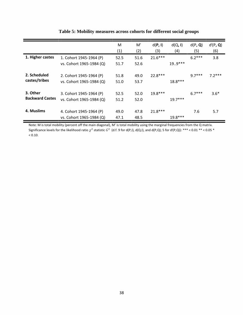
38
Table 5: Mobility measures across cohorts for different social groups
M M' d(P, I) d(Q, I) d(P, Q) di(P, Q)
(1) (2) (3) (4) (5) (6)
1. Higher castes 1. Cohort 1945-1964 (P) 52.5 51.6 21.6***
6.2*** 3.8
vs. Cohort 1965-1984 (Q) 51.7 52.6
19..9***
2. Scheduled castes/tribes
2. Cohort 1945-1964 (P) 51.8 49.0 22.8***
9.7*** 7.2***
vs. Cohort 1965-1984 (Q) 51.0 53.7
18.8***
3. Other Backward Castes
3. Cohort 1945-1964 (P) 52.5 52.0 19.8***
6.7*** 3.6*
vs. Cohort 1965-1984 (Q) 51.2 52.0
19.7***
4. Muslims 4. Cohort 1945-1964 (P) 49.0 47.8 21.8***
7.6 5.7
vs. Cohort 1965-1984 (Q) 47.1 48.5
19.8***
Note: M is total mobility (percent off the main diagonal), M’ is total mobility using the marginal frequencies from the Q matrix.
Significance levels for the likelihood ratio 𝜒2 statistic 𝐺2 (d.f. 9 for d(P,I), d(Q,I), and d(P,Q); 5 for di(P,Q)): *** < 0.01 ** < 0.05 *
< 0.10.

39
Table 6: Components of d(P,I), d(Q,I), and d(P,Q) for sons’ birth cohort 1945-64 (P) vs. birth
cohort 1965-84 (Q) for different social groups
Contrast d(P,I) Odds ratio
d(Q,I) Odds ratio
d(P,Q) Percentage of total
Cumulative percentage
Social Group: Higher Castes
1. [(WF)/(WU)]/[(UF)/(UU)] 1.16* 1.79 3.47*** 5.66 2.30*** 13.82 13.82
2. [(SF)/(SU)]/[(UF)/(UU)] 0.58 0.75 1.47*** 2.09 2.05*** 10.99 24.80
3. [(WF)/(WU)]/[(FF)/(FU)] 2.43*** 0.30 0.62 0.73 1.81** 8.53 33.33
4. [(FF)/(FS)]/[(SF)/(SS)] 7.96*** 53.42 6.17*** 21.92 1.78*** 8.26 41.58
5. [(FW)/(FF)]/[(SW)/(SF)] 7.13*** 0.03 5.45*** 0.07 1.68*** 7.33 48.91
6. [(SF)/(SS)]/[(UF)/(US)] 4.84*** 0.09 3.26*** 0.20 1.59*** 6.56 55.48
7. [(FF)/(FU)]/[(SF)/(SU)] 4.18*** 8.07 2.61*** 3.70 1.56** 6.34 61.81
8. [(SW)/(SF)]/[(UW)/(UF)] 4.42*** 9.10 2.89*** 4.24 1.53** 6.06 67.87
9. [(WF)/(WS)]/[(FF)/(FS)] 4.97*** 0.08 3.50*** 0.17 1.47*** 5.65 73.51
Social Group: Scheduled Castes/Tribes
1. [(WW)/(WF)]/[(FW)/(FF)] 8.30*** 63.48 5.06*** 12.56 3.24** 11.28 11.28
2. [(FW)/(FF)]/[(SW)/(SF)] 6.36*** 0.04 3.14*** 0.21 3.22*** 11.12 22.41
3. [(WF)/(WU)]/[(FF)/(FU)] 2.50** 0.29 0.39 1.22 2.89** 8.98 31.39
4. [(WF)/(WS)]/[(UF)/(US)] 1.85* 0.40 1.01* 1.65 2.86** 8.77 40.15
5. [(WF)/(WS)]/[(FF)/(FS)] 4.96*** 0.08 2.19*** 0.33 2.77** 8.23 48.39
6. [(WW)/(WF)]/[(UW)/(UF)] 5.37*** 14.69 2.72*** 3.89 2.66** 7.59 55.98
7. [(SW)/(SF)]/[(UW)/(UF)] 3.43*** 5.55 0.79* 1.49 2.64*** 7.46 63.44
8. [(WF)/(WU)]/[(UF)/(UU)] 1.92 2.62 4.54*** 9.68 2.62** 7.36 70.81
9. [(FF)/(FU)]/[(SF)/(SU)] 3.25*** 5.09 0.71** 1.43 2.54*** 6.95 77.75
10. [(SF)/(SS)]/[(UF)/(US)] 3.51*** 0.17 0.99*** 0.61 2.52*** 6.82 84.58
11. [(FF)/(FS)]/[(SF)/(SS)] 6.62*** 27.36 4.19*** 8.11 2.43*** 6.35 90.93
12. [(SF)/(SU)]/[(UF)/(UU)] 1.17* 1.80 3.44*** 5.58 2.27*** 5.53 96.47
Social Group: Other Backward castes
1. [(SF)/(SU)]/[(UF)/(UU)] 1.02** 1.66 3.03*** 4.54 2.01*** 9.09 9.09
2. [(FW)/(FF)]/[(SW)/(SF)] 6.32*** 0.04 4.36*** 0.11 1.96*** 8.62 17.71
3. [(FF)/(FS)]/[(SF)/(SS)] 7.08*** 34.44 5.22*** 13.63 1.85*** 7.73 25.43
4. [(FF)/(FU)]/[(SF)/(SU)] 3.28*** 5.14 1.43*** 2.04 1.85*** 7.67 33.11
5. [(WW)/(WF)]/[(SW)/(SF)] 0.04 0.98 1.66*** 2.30 1.70* 6.51 39.62
6. [(WF)/(WS)]/[(FF)/(FS)] 4.78*** 0.09 3.10*** 0.21 1.68** 6.37 45.99
7. [(WW)/(WU)]/[(UW)/(UU)] 5.15*** 13.16 6.83*** 30.48 1.68** 6.34 52.33
8. [(WW)/(WS)]/[(SW)/(SS)] 2.26*** 3.10 3.79*** 6.66 1.53** 5.27 57.60
9. [(SW)/(SF)]/[(UW)/(UF)] 3.05*** 4.59 1.53*** 2.15 1.52*** 5.18 62.78
10.[(WF)/(WU)]/[(UF)/(UU)] 2.14*** 2.92 3.64*** 6.18 1.50* 5.03 67.81
Social Group: Muslims
1. [(WW)/(WF)]/[(FW)/(FF)] 8.20*** 60.23 5.42*** 14.99 2.78* 13.49 13.49
2. [(WF)/(WU)]/[(UF)/(UU)] 1.97 2.68 4.41*** 9.05 2.44 10.36 23.84
3. [(WF)/(WS)]/[(FF)/(FS)] 5.28*** 0.07 2.85*** 0.24 2.43* 10.31 34.15

40
4. [(WF)/(WS)]/[(UF)/(US)] 1.27 0.53 1.14*** 1.77 2.40 10.06 44.21
5. [(WF)/(WU)]/[(FF)/(FU)] 2.66* 0.26 0.29*** 0.87 2.38 9.86 54.07
6. [(FW)/(FF)]/[(SW)/(SF)] 6.44*** 0.04 4.34*** 0.11 2.10*** 7.71 61.77
7. [(WW)/(WF)]/[(UW)/(UF)] 3.91*** 7.07 2.08*** 2.83 1.83 5.82 67.59
Notes: First element of each pair is father’s occupation, second is son’s. W: White Collar, S: Skilled/Semi-skilled, U: Unskilled, F: Farmer. Significance levels for the likelihood ratio 𝜒2 statistic 𝐺2. *** < 0.01 ** < 0.05 * < 0.10.

41
Table 7: Comparison of mobility of each social group
to total population mobility
Panel 1: Son's Birth Cohort=1945-64
M M' d(P, I) d(Q, I) d(P, Q) di(P, Q)
(1) (2) (3) (4) (5) (6)
1. Higher castes (P) 52.5 53.8 21.6***
3.8* 2.3
vs. All (Q) 51.9 51.2
21.9***
2. SC/ST (P) 51.8 51.7 22.8
3.3 1.6
vs. All (Q) 51.9 52.1
21.9***
3.OBC (P) 52.5 53.4 19.8***
3.2 1.1
vs. All (Q) 51.9 51.2
21.9***
4. Muslims (P) 50.0 52.5 21.8***
3.8 3.4
vs. All (Q) 51.9 48.4
21.9*** Panel 2: Son's Birth Cohort=1965-84
M M' d(P, J) d(Q, J) d(P, Q) di(P, Q)
(1) (2) (3) (4) (5) (6)
1. Higher castes (P) 51.7 51.8 19.9***
3.7*** 3.0**
vs. All (Q) 50.8 50.8
20.3***
2. SC/ST (P) 51.0 53.4 18.8***
3.4*** 2.2
vs. All (Q) 50.8 48.8
20.3***
3.OBC (P) 51.2 51.2 19.7***
1.9 1.8
vs. All (Q) 50.8 50.8
20.3***
4. Muslims (P) 47.1 50.1 19.8***
2.9 2.0
vs. All (Q) 50.8 47.5
20.3***
Note: M is total mobility (percent off the main diagonal), M’ is total mobility using the marginal frequencies from the
Q matrix. Significance levels for the likelihood ratio χ^2 statistic G^2 (d.f. 9 for d(P,I), d(Q,I), and d(P,Q); 5 for di(P,Q)):
*** < 0.01 ** < 0.05 * < 0.10.

42
Table 8: Comparison of mobility of disadvantage groups
to higher castes mobility
Panel I: Son's Birth Cohort=1945-64
M M' d(P, I) d(Q,I) d(P, Q) di(P, Q)
(1) (2) (3) (4) (5) (6)
1. SC/ST (P) 51.8 50.7 22.8*** 5.7** 2.5
(54.2)
2.OBC (P) 52.5 53.0 19.8*** 4.1 2.5
(52.9)
3. Muslims (P) 49.0 51.4 21.8*** 6.2 5.4
(50.0)
vs. Higher castes (Q) 52.5 21.6***
Panel 2: Son's Birth Cohort=1965-84
M M' d(P, I) d(Q, I) d(P, Q) di(P, Q)
(1) (2) (3) (4) (5) (6)
1. SC/ST (P) 51.0 53.4 18.8***
6.5*** 5.1***
(49.8)
2.OBC (P) 51.2 51.1 19.7***
4.2** 3.8**
(51.6)
3. Muslims (P) 47.1 50.4 19.8***
4.8* 4.7*
(48.3)
vs. Higher castes (Q) 51.7
19.9***
Note: M is total mobility (percent off the main diagonal), M’ is total mobility using the marginal frequencies from the
Q matrix. The numbers in parenthesis are mobility in Q using marginal frequencies from P. Significance levels for the
likelihood ratio 𝜒2 statistic 𝐺2 (d.f. 9 for d(P,I), d(Q,I), and d(P,Q); 5 for di(P,Q)): *** < 0.01 ** < 0.05 * < 0.10.

43
Table 9: Components of d(P,I), d(Q,I), and d(P,Q) for SC/ST (P) vs. higher castes (Q)
Panel 1: Birth Cohort 1945-1964
Contrast
d(P,I) Odds ratio
d(Q,I) Odds ratio
d(P,Q) Percentage of total
Cumulative percentage
1. [(WW)/(WF)]/[(SW)/(SF)] 1.9 2.6 0.1 0.9 2.1 12.9 12.9
2. [(WW)/(WU)]/[(UW)/(UU)] 7.3*** 38.4 5.5*** 15.4 1.8** 10.2 23.2
3. [(SF)/(SU)]/[(UF)/(UU)] 1.2* 1.8 0.6 0.7 1.8** 9.4 32.6
4. [(FF)/(FS)]/[(SF)/(SS)] 6.6*** 27.4 8.0*** 53.4 1.3* 5.5 38.1
5. [(SF)/(SS)]/[(UF)/(US)] 3.5*** 0.2 4.8*** 0.1 1.3 5.5 43.6
6. [(WF)/(WS)]/[(SF)/(SS)] 1.7 2.3 3.0*** 4.5 1.3 5.4 49.0
7. [(WW)/(WS)]/[(FW)/(FS)] 3.3*** 5.3 2.1*** 2.8 1.3** 5.1 54.1
8. [(WW)/(WF)]/[(FW)/(FF)] 8.3*** 63.5 7.0*** 33.6 1.3 5.0 59.1
9. [(WW)/(WU)]/[(FW)/(FU)] 5.8*** 18.2 4.6*** 10.0 1.2 4.5 63.5
10.[(WW)/(WS)]/[(UW)/(US)] 3.5*** 5.8 2.5*** 3.4 1.1* 3.5 67.1
11.[(WW)/(WF)]/[(UW)/(UF)] 5.4*** 14.7 4.3*** 8.6 1.1 3.5 70.5
12.[(WW)/(WU)]/[(SW)/(SU)] 2.7*** 3.9 1.6*** 2.3 1.1 3.5 74.0
13.[(WF)/(WU)]/[(SF)/(SU)] 0.8 1.5 1.7** 2.4 1.0 3.0 77.0
Panel 2: Birth Cohort 1965-84
1. [(FW)/(FF)]/[(SW)/(SF)] 3.1*** 0.2 5.5*** 0.1 2.3*** 12.7 12.7
2. [(SF)/(SS)]/[(UF)/(US)] 1.0*** 0.6 3.3*** 0.2 2.3*** 12.1 24.8
3. [(SW)/(SF)]/[(UW)/(UF)] 0.8* 1.5 2.9*** 4.2 2.1*** 10.4 35.2
4. [(FF)/(FS)]/[(SF)/(SS)] 4.2*** 8.1 6.2*** 21.9 2.0*** 9.4 44.6
5. [(SF)/(SU)]/[(UF)/(UU)] 3.4*** 5.6 1.5*** 2.1 2.0*** 9.1 53.7
6. [(FF)/(FU)]/[(SF)/(SU)] 0.7** 1.4 2.6*** 3.7 1.9*** 8.6 62.3
7. [(WW)/(WF)]/[(SW)/(SF)] 1.9*** 2.6 0.3*** 1.2 1.6*** 6.1 68.4
8. [(WF)/(WS)]/[(UF)/(US)] 1.0* 1.7 0.6*** 0.7 1.6** 5.9 74.3
9. [(WF)/(WS)]/[(FF)/(FS)] 2.2*** 0.3 3.5*** 0.2 1.3** 4.0 78.3
Notes: First element of each pair is father’s occupation, second is son’s. W: White Collar, S: Skilled/Semi-
skilled, U: Unskilled, F: Farmer. Significance levels for the likelihood ratio 𝜒2 statistic 𝐺2. *** < 0.01 ** <
0.05 * < 0.10.
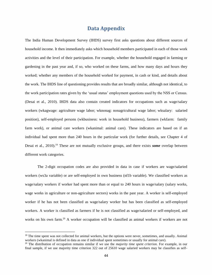
44
Data Appendix
The India Human Development Survey (IHDS) survey first asks questions about different sources of
household income. It then immediately asks which household members participated in each of those work
activities and the level of their participation. For example, whether the household engaged in farming or
gardening in the past year and, if so, who worked on these farms, and how many days and hours they
worked; whether any members of the household worked for payment, in cash or kind, and details about
the work. The IHDS line of questioning provides results that are broadly similar, although not identical, to
the work participation rates given by the ‘usual status’ employment questions used by the NSS or Census.
(Desai et al., 2010). IHDS data also contain created indicators for occupations such as wage/salary
workers (wkagwage: agriculture wage labor; wknonag: nonagricultural wage labor; wksalary: salaried
position), self-employed persons (wkbusiness: work in household business), farmers (wkfarm: family
farm work), or animal care workers (wkanimal: animal care). These indicators are based on if an
individual had spent more than 240 hours in the particular work (for further details, see Chapter 4 of
Desai et al., 2010).19 These are not mutually exclusive groups, and there exists some overlap between
different work categories.
The 2-digit occupation codes are also provided in data in case if workers are wage/salaried
workers (ws3a variable) or are self-employed in own business (nf1b variable). We classified workers as
wage/salary workers if worker had spent more than or equal to 240 hours in wage/salary (salary works,
wage works in agriculture or non-agriculture sectors) works in the past year. A worker is self-employed
worker if he has not been classified as wage/salary worker but has been classified as self-employed
workers. A worker is classified as farmers if he is not classified as wage/salaried or self-employed, and
works on his own farm.20 A worker occupation will be classified as animal workers if workers are not
19 The time spent was not collected for animal workers, but the options were never, sometimes, and usually. Animal
workers (wkanimal is defined in data as one if individual spent sometimes or usually for animal care). 20 The distribution of occupation remains similar if we use the majority time spent criterion. For example, in our
final sample, if we use majority time criterion 322 out of 25610 wage salaried workers may be classifies as self-

45
classified in the first three categories, and reported to have taken care of animals usually.21 In case of
wage salaried workers and self-employed workers, we used the 2-digit occupation codes given in data
(ws3a and nf1b) to disaggregate workers, while for farmers and animal care workers; we imputed the two
digits codes (62: who work on own farm, and 65: animal care workers). Once we have two digit
occupation codes for all workers, we use those to reclassify in four groups of workers (white collar,
skilled/semi-skilled, unskilled, and farmers).22
To get the occupation of fathers, we use following information (see appendix1, Table 1).
First, majority of adult male members are heads of the household and their fathers are not living
in the same household (except for few cases). The IHDS data collected information about
occupation and education of father/husband of household head---Question 1.19 and 1.20 on page
3 of household questionnaire (id19 and id20 variable in data). As our sample is restricted to
men, the id19 variable provides information about occupation of fathers of the heads.23 Second,
the fathers of few individuals, especially for the younger men, live in the same household (parent
id reported in data), and hence we know their occupation if they have reported working. Third,
we exploit relation to head variable to get fathers occupation for some individuals. For example,
employed workers. The overlap with farmers is somewhat higher. However, on closer look, majority of these
overlap is because of agriculture labor/daily workers who work for wages (hence classified as wage/salary workers) working on their own farm also. These individuals are more likely marginal farmers and closer to agricultural
laborers than farmers. Hence we preferred to categorize them as reported through wage earning status rather than
farmers. 21 For animal care work, there is no number of days or hours reported. However, question 5.5 (variable an6 in data)
on page 10 of household questionnaire asks how often the person take care of the animals with possible answer of
never, sometimes, or usually. The IHDS data provide a category wkanimal: animal care worker if the worker take
care of animals sometimes or usually. IHDS data define people as working (wkany variable in data) if they were
engaged for at least 240 hours during the preceding year in one or more gainful activities, such as working in
household farms or businesses, or for a wage or salary, or persons who sometimes or usually take care of animals.
However, we only classified those workers as animal care workers who were not classified as wage/salary, self-
employed business, or farmers based on 240 hours work criterion and reported that they usually take care of
animals. As a result the number of workers based on our categories is lower than number of workers based on IHDS
data wkany indicator. 22 See appendix 2 for exact reclassification. 23 Id19b variable in data provide text description of the occupation. The author found few discrepancies in id19
variable based on id19b description, and corrected accordingly few cases where the discrepancy seems obvious, e.g.,
in few cases text description says agriculture labor, while the id19 is coded as 3 (3: Engineering Technicians)
whereas the actual code for agricultural laborers is 63.

46
if an individuals has reported as brother of head (male headed households) of the household, for
that individual, the father is same person as household head’s father (for who, we have
information from id19 variable).
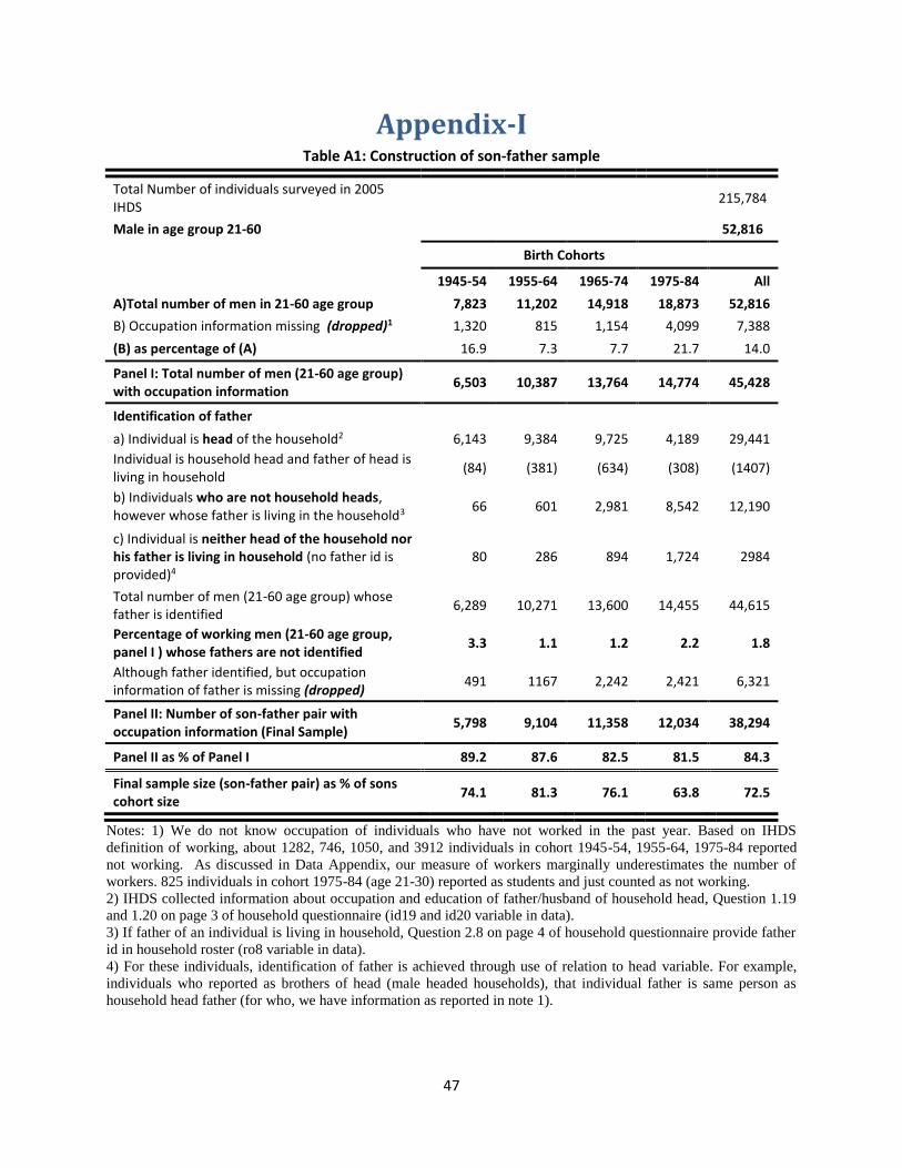
47
Appendix-I Table A1: Construction of son-father sample
Total Number of individuals surveyed in 2005 IHDS
215,784
Male in age group 21-60 52,816
Birth Cohorts
1945-54 1955-64 1965-74 1975-84 All
A)Total number of men in 21-60 age group 7,823 11,202 14,918 18,873 52,816
B) Occupation information missing (dropped)1 1,320 815 1,154 4,099 7,388
(B) as percentage of (A) 16.9 7.3 7.7 21.7 14.0
Panel I: Total number of men (21-60 age group) with occupation information
6,503 10,387 13,764 14,774 45,428
Identification of father
a) Individual is head of the household2 6,143 9,384 9,725 4,189 29,441
Individual is household head and father of head is living in household
(84) (381) (634) (308) (1407)
b) Individuals who are not household heads, however whose father is living in the household3
66 601 2,981 8,542 12,190
c) Individual is neither head of the household nor his father is living in household (no father id is provided)4
80 286 894 1,724 2984
Total number of men (21-60 age group) whose father is identified
6,289 10,271 13,600 14,455 44,615
Percentage of working men (21-60 age group, panel I ) whose fathers are not identified
3.3 1.1 1.2 2.2 1.8
Although father identified, but occupation information of father is missing (dropped)
491 1167 2,242 2,421 6,321
Panel II: Number of son-father pair with occupation information (Final Sample)
5,798 9,104 11,358 12,034 38,294
Panel II as % of Panel I 89.2 87.6 82.5 81.5 84.3
Final sample size (son-father pair) as % of sons cohort size
74.1 81.3 76.1 63.8 72.5
Notes: 1) We do not know occupation of individuals who have not worked in the past year. Based on IHDS
definition of working, about 1282, 746, 1050, and 3912 individuals in cohort 1945-54, 1955-64, 1975-84 reported
not working. As discussed in Data Appendix, our measure of workers marginally underestimates the number of
workers. 825 individuals in cohort 1975-84 (age 21-30) reported as students and just counted as not working.
2) IHDS collected information about occupation and education of father/husband of household head, Question 1.19
and 1.20 on page 3 of household questionnaire (id19 and id20 variable in data).
3) If father of an individual is living in household, Question 2.8 on page 4 of household questionnaire provide father
id in household roster (ro8 variable in data).
4) For these individuals, identification of father is achieved through use of relation to head variable. For example,
individuals who reported as brothers of head (male headed households), that individual father is same person as
household head father (for who, we have information as reported in note 1).

48
Table A2: Summary Measures of Mobility using nine occupation groups
M M' d(P, I) d(Q,I) d(P, Q) di(P, Q)
(1) (2) (3) (4) (5) (6)
1. Cohort 1945-1954 (P) 44.7 50.3 110.2*** 57.6 55.8
vs. Cohort 1955-1964 (Q) 50.7 45.1 104.3***
2. Cohort 1955-1964 (P) 50.7 52.4 104.2*** 41.1 40.4
vs. Cohort 1965-1974 (Q) 52.7 50.8 98.8***
3. Cohort 1965-1974 (P) 52.7 48.6 98.8*** 40.1*** 35.6
vs. Cohort 1975-1984 (Q) 48.2 52.6 98.8***
4. Cohort 1945-1954 (P) 44.7 47.2 110.2*** 58.2*** 54.0***
vs. Cohort 1975-1984 (Q) 48.2 45.6 98.8***
Note: M is total mobility (percent off the main diagonal), M’ is total mobility using the marginal frequencies from the Q
matrix. Significance levels for the likelihood ratio 𝜒2 statistic 𝐺2 (d.f. 64 for d(P,J), d(Q,J), and d(P,Q); and 56 for di(P,Q).
*** < 0.01 ** < 0.05 * < 0.10.

49
Appendix 2: Classification of occupation
White Collar Skilled/Semi-Skilled NCAER
Occupation Code Description
NCAER Occupation
Code Description
Division 0-1: PROFESSIONAL and TECHNICAL Division 3: CLERICAL
0 Physical Scientists 30 Clerical, Transport, and Communication Supervisors
1 Physical Science Technicians 31 Village Officials
2 Architects, Engineers, Technologists and Surveyors 32 Stenographers and Typists
3 Engineering Technicians 33 Book-keepers, Cashiers and Related Workers
4 Aircraft and Ships Officers 34 Computing Machine Operators
5 Life Scientists 35 Clerical and Related Workers, n.e.c.
6 Life Science Technicians 36 Transport and Communication Supervisors
7 Physicians and Surgeons 37 Transport Conductors and Guards
8 Nursing and other Health Technicians 38 Mail Distributors and Related Workers
9 Scientific, Medical and Technical Persons, Other 39 Telephone and Telegraph Operators
10 Mathematicians, Statisticians and Related Workers Division 4: SALES
11 Economists and Related Workers 40 Merchants and Shopkeepers, Wholesale and Retail Trade
12 Accountants, Auditors and Related Workers 41 Manufacturers, Agents
13 Social Scientists and Related Workers 42 Technical Sales and Commercial Travellers
14 Jurists 43 Sales, Shop Assistants and Related Workers
15 Teachers 44 Insurance, Real Estate, Securities and Business Service Sales
16 Poets, Authors, Journalists and Related Workers 45 Money Lenders and Pawn Brokers
17 Sculptors, Photographers and Creative Artists 49 Sales Workers, n.e.c.
18 Composers and Performing Artists Division 7-8-9: PRODUCTION, TRANSPORT EQUIPMENT, and LABOURERS (Labourers-99, are classified in unskilled group)
19 Professional Workers, n.e.c. 71 Miners, Quarrymen, Well Drillers and Related Workers
Division 2: MANAGERS 72 Metal Processors
20 Elected and Legislative Officials 73 Wood Preparation Workers and Paper Makers
21 Administrative Officials Government and Local Bodies 74 Chemical and Related Workers
22 Managers and Working Proprietors, Wholesale and Retail Trade 75 Spinners, Weavers, Knitters, Dyers and Related Workers
23 Managers and Directors, Financial Institutions 76 Tanners, Fellmongers and Pelt Dressers
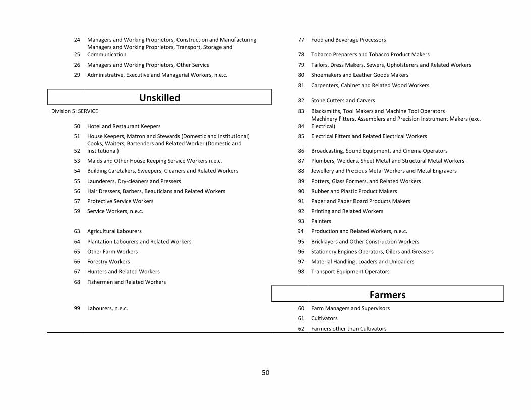
50
24 Managers and Working Proprietors, Construction and Manufacturing 77 Food and Beverage Processors
25 Managers and Working Proprietors, Transport, Storage and Communication 78 Tobacco Preparers and Tobacco Product Makers
26 Managers and Working Proprietors, Other Service 79 Tailors, Dress Makers, Sewers, Upholsterers and Related Workers
29 Administrative, Executive and Managerial Workers, n.e.c. 80 Shoemakers and Leather Goods Makers
81 Carpenters, Cabinet and Related Wood Workers
Unskilled 82 Stone Cutters and Carvers
Division 5: SERVICE 83 Blacksmiths, Tool Makers and Machine Tool Operators
50 Hotel and Restaurant Keepers 84 Machinery Fitters, Assemblers and Precision Instrument Makers (exc. Electrical)
51 House Keepers, Matron and Stewards (Domestic and Institutional) 85 Electrical Fitters and Related Electrical Workers
52 Cooks, Waiters, Bartenders and Related Worker (Domestic and Institutional) 86 Broadcasting, Sound Equipment, and Cinema Operators
53 Maids and Other House Keeping Service Workers n.e.c. 87 Plumbers, Welders, Sheet Metal and Structural Metal Workers
54 Building Caretakers, Sweepers, Cleaners and Related Workers 88 Jewellery and Precious Metal Workers and Metal Engravers
55 Launderers, Dry-cleaners and Pressers 89 Potters, Glass Formers, and Related Workers
56 Hair Dressers, Barbers, Beauticians and Related Workers 90 Rubber and Plastic Product Makers
57 Protective Service Workers 91 Paper and Paper Board Products Makers
59 Service Workers, n.e.c. 92 Printing and Related Workers
93 Painters
63 Agricultural Labourers 94 Production and Related Workers, n.e.c.
64 Plantation Labourers and Related Workers 95 Bricklayers and Other Construction Workers
65 Other Farm Workers 96 Stationery Engines Operators, Oilers and Greasers
66 Forestry Workers 97 Material Handling, Loaders and Unloaders
67 Hunters and Related Workers 98 Transport Equipment Operators
68 Fishermen and Related Workers
Farmers 99 Labourers, n.e.c. 60 Farm Managers and Supervisors
61 Cultivators
62 Farmers other than Cultivators