interfacing simulink/matlab with v-rep for analysis...

INTERFACING SIMULINK/MATLAB WITH V-REP FOR ANALYSIS AND

CONTROL SYNTHESIS OF A QUADROTOR

A THESIS SUBMITTED TO

THE GRADUATE SCHOOL OF NATURAL AND APPLIED SCIENCES

OF

MIDDLE EAST TECHNICAL UNIVERSITY

BY

JAVID KHALILOV

IN PARTIAL FULFILLMENT OF THE REQUIREMENTS

FOR

THE DEGREE OF MASTER OF SCIENCE

IN

AEROSPACE ENGINEERING

MAY 2016

Approval of the thesis:



submitted by JAVID KHALILOV in partial fulfillment of the requirements for the

degree of Master of Science in Aerospace Engineering Department, Middle East

Technical University by,

Prof. Dr. Gülbin Dural Ünver ____________________

Dean, Graduate School of Natural and Applied Sciences

Prof. Dr. Ozan Tekinalp _____________________

Head of Department, Aerospace Engineering

Asst. Prof. Dr. Ali Türker Kutay _____________________

Supervisor, Aerospace Engineering Dept., METU

Examining Committee Members:

Prof. Dr. Ozan Tekinalp _____________________

Aerospace Engineering Dept., METU

Asst. Prof. Dr. Ali Türker Kutay _____________________


Assoc. Prof. Dr. Dilek Funda Kurtuluş _____________________


Asst. Prof. Dr. Yusuf Sahillioğlu _____________________

Computer Engineering Dept., METU

Asst. Prof. Dr. Ali Ruhşen Çete _____________________

Dept. of Aeronautical Science, GAZÜ

Date: 05.05.2016

iv

I hereby declare that all information in this document has been obtained and

presented in accordance with academic rules and ethical conduct. I also declare

that, as required by these rules and conduct, I have fully cited and referenced all

material and results that are not original to this work.

Name, Last Name : Javid KHALILOV

Signature :

v

ABSTRACT



Khalilov, Javid

M.S., Department of Aerospace Engineering

Supervisor: Asst. Prof. Dr. Ali Türker Kutay

May 2016, 79 pages

The primary factor that restricts the new control systems developments for air vehicles

and the implementation of various sensors for advanced algorithms is the deficiency

of quick and cost-effective physical environment. Flight tests are costly and requires a

long preparation process. The aim of this thesis is to improve the simulator

infrastructure which easily implementable to the AscTec Hummingbird Quadrotor that

is located in the University’s lab and have interaction with the 3D physical

environment. Firstly, quadrotor’s mathematical model has been developed and this

model is implemented on Matlab/Simulink environment. Afterwards, a basic PID

controller is developed for attitude control. The quadrotor’s physical model, the

electric motor, the rotor and the IMU model have been modelled on Virtual Robotics

Experimentation Platform (V-REP). Matlab / Simulink controller is synchronized with

the V-REP and is used for the quadrotor’s physical environment tests. The verification

of the simulation is done by real experimental flight data of AscTec Hummingbird.

The collision avoidance and wall following algorithms in empty room using ultrasonic

distance sensors are implemented to show the usefulness of simulator infrastructure.

vi

Keywords: Quadrotor, PID Controller, Simulink/Matlab, V-REP, Dynamic model,

System verification, Ultrasonic distance sensors, Collision avoidance, Wall following

vii

ÖZ

DÖRT ROTORLU HAVA ARACI ANALİZİ VE KONTROLCÜ SENTEZİ İÇİN

SIMULINK/MATLAB VE V-REP ENTEGRASYONU

Khalilov, Javid

Yüksek Lisans, Havacılık ve Uzay Mühendisliği Bölümü

Tez Yöneticisi: Yrd. Doç. Dr. Ali Türker Kutay

Mayıs 2016, 79 sayfa

Hava araçlarındaki yeni kontrol sistemi denemeleri ve yeni sensör implementasyonunu

kısıtlayan başlıca etken fiziksel olarak hızlı ve ucuz test yapamama durumudur. Uçuş

testleri maliyetli ve uzun hazırlanma süreci istemektedir. Bu tez çalışmasındaki amaç

üniversite labında bulunan AscTec Hummingbird dört rotorlu hava aracı için kolay

uygulanabilen ve 3D fiziksel ortamla etkileşimde olan bir simülatör altyapısı

geliştirmektir. İlkin olarak dört rotorlu hava aracının matematik modelini çıkarılmış

ve Matlab/Simulink ortamında simüle edilmiştir. Matematik model implemente

edildikten sonra basit bir PID kontrolcü geliştirilmiştir. Dört rotorlu hava aracı fiziksel

modeli, elektrik motor ve pervane ve IMU modeli Virtual Robotics Experimentation

Platform (V-REP) ‘de modellenmiştir. Matlab/Simulink kontrolcüsü V-REP ile

senkronize edilmiş ve quadrotorun fiziksel ortam testleri için kullanılmıştır.

Simülasyon sağlaması quadrotorun yazılımı kullanılarak yapılan deney verileri ile

sağlanmıştır. Simülatör altyapısının uygulanabilirliğini göstermek amaçlı ultrasonik

mesafe sensörleri kullanılarak engel sakınma ve boş odada duvar takibi çalışmaları

yapılmıştır.

viii

Anahtar Kelimeler: Dört rotorlu hava aracı, PID kontrolcü, Simulink/Matlab, V-

REP, Dinamik model, Simülasyon sağlaması, Ultrasonik mesafe sensörü, Engel

sakınma, Duvar takibi

ix

to my parents...

x

ACKNOWLEDGMENTS

I would like to express my deepest gratitude to my supervisor Assoc. Prof. Dr. Ali

Türker Kutay for all the opportunities he provided to me during all stages of this study.

I am grateful to him for his sincere and valuable guidance.

I would like to thank Mustafa Çağlayan Durmaz, İlker Moral for their support and

creating comfortable environment to me to work. I would like to thank Engin Esin for

his support and discussions.

I am very grateful to Eda Önerli for always being with me, encouragement and

limitless support.

xi

TABLE OF CONTENTS

Table of Contents

ABSTRACT ................................................................................................................. v

ÖZ ........................................................................................................................... vii

ACKNOWLEDGMENTS ........................................................................................... x

TABLE OF CONTENTS ............................................................................................ xi

LIST OF TABLES .................................................................................................... xiii

LIST OF FIGURES .................................................................................................. xiv

NOMENCLATURE ................................................................................................ xviii

CHAPTERS

1. INTRODUCTION ................................................................................... 1

1.1 Background Information ...................................................................... 1

1.2 Present Approach.................................................................................. 1

1.3 Major Objectives .................................................................................. 9

1.4 Literature Survey .................................................................................. 9

1.5 Outline of the Thesis .......................................................................... 15

2. QUADROTOR SETUP ......................................................................... 17

2.1 Quadrotor Properties .......................................................................... 17

2.2 AscTec Simulink Toolkit Overview and Connections ....................... 19

3. MATHEMATICAL MODEL AND CONTROLLER DESIGN ........... 23

3.1 Mathematical Model of Quadrotor ..................................................... 23

3.2 PID Controller Design ........................................................................ 27

4. V-REP MODEL AND MATLAB/SIMULINK INTERFACING ......... 31

4.1 Virtual Robot Experimentation Platform (V-REP) ............................ 31

4.2 Propeller Model in V-REP ................................................................. 36

4.3 Quadrotor Model in V-REP................................................................ 37

4.4 Simulink/Matlab and V-REP Interfacing ........................................... 39

xii

5. SIMULATION RESULTS ..................................................................... 41

5.1 Simulation Results of Simulink/Matlab and V-REP Integration ........ 41

5.2 Experimental Setup for Quadrotor Flight Test ................................... 47

5.3 Controller Design and Implementation on Real Quadrotor ................ 51

5.4 Experimental Data and Case Comparison with Simulation Data ....... 53

5.5 Collision Avoidance and Wall Following .......................................... 59

6. CONCLUSION AND FUTURE WORK ............................................... 75

REFERENCES ........................................................................................................... 77

xiii

LIST OF TABLES

TABLES

Table 2.1. AscTec Hummingbird Properties [19]. ..................................................... 18

Table 5.1.Tuned PID gains......................................................................................... 41

xiv

LIST OF FIGURES

FIGURES

Figure 1.1.STARMAC II [2]. ....................................................................................... 3

Figure 1.2.MARK II X4 Flyer [3]. ............................................................................... 4

Figure 1.3.ETH Zurich research quadrotor [4]. ........................................................... 4

Figure 1.4.Micro quadrotor in University of Pennsylvania Grasp Lab [5]. ................. 5

Figure 1.5.Variable pitch quadrotor in MIT [6]. .......................................................... 6

Figure 1.6. Some popular commercial quadrotors in market ...................................... 8

Figure 1.7. Flight test area built for AscTec Hummingbird experiments [13]. .......... 11

Figure 1.8. Motor response to oscillating roll stick input [13]. .................................. 11

Figure 1.9. Motor response to oscillating pitch stick input [13]. ............................... 12

Figure 1.10. Handlebar position ad vehicle linear speed response on real vehicle and

V-REP simulation [14]. .............................................................................................. 13

Figure 1.11. The control and communication scheme of PyQuadSim [16]. .............. 13

Figure 1.12. The V-REP, ROS and Simulink software flow diagram [17]................ 14

Figure 1.13. Response of three axis fuzzy logic controller working together to step

input in simulation [18]. ............................................................................................. 15

Figure 1.14. Response of three axis fuzzy logic controller against disturbances in real

[18]. ............................................................................................................................ 15

Figure 2.1. AscTec Hummingbird quadrotor [13]. .................................................... 18

Figure 2.2. AscTec Autopilot general scheme [20] ................................................... 19

Figure 2.3. The onboard_matlab.mdl Simulink model scheme ................................ 20

Figure 2.4. UART_Communication.mdl Simulink model scheme ........................... 21

Figure 3.1.Free body diagram of quadrotor [21] ........................................................ 23

Figure 3.2.Yaw PID controller scheme ...................................................................... 28

Figure 3.3.Roll PID controller scheme ....................................................................... 28

Figure 3.4.Pitch PID Controller scheme .................................................................... 29

Figure 3.5.Altitude PID controller ............................................................................. 29

Figure 4.1.The built-in V-REP robot models ............................................................. 33

Figure 4.2.The remote API communication modes: (a) blocking function call, (b) non-

blocking function call [22]. ........................................................................................ 35

xv

Figure 4.3.(a) Thrust change w.r.t. the angular velocity of the rotor using BET in

hovering flight, (b) Rotor torque change w.r.t. the angular velocity of the rotor using

BET in hovering flight [27]........................................................................................ 36

Figure 4.4.Propeller model in V-REP ........................................................................ 37

Figure 4.5.General AscTec Hummingbird quadrotor view in V-REP ....................... 38

Figure 4.6.General simulator operation diagram ....................................................... 40

Figure 5.1.Motor throttle command (%) and rotation speed (rpm) during hover flight

simulation. .................................................................................................................. 42

Figure 5.2.Roll, pitch and yaw angles of quadrotor during hover flight simulation. The

10 degrees roll doublet input is shown in dashed lines. ............................................. 42

Figure 5.3.Roll, pitch and yaw angular rates change during hover flight simulation. 43

Figure 5.4.The u, v and w velocities during hover flight simulation. ........................ 43

Figure 5.5. The x, y and z positions of the quadrotor during hover flight simulation.

The z command is shown in dashed lines. ................................................................. 44


simulation with ground disturbance take-off. ............................................................ 44

Figure 5.7.Roll, pitch and yaw angles of quadrotor during hover flight simulation with

ground disturbance take-off. The 10 degrees roll doublet input is shown in dashed

lines. ........................................................................................................................... 45

Figure 5.8.Roll, pitch and yaw angular rates change during hover flight simulation with

ground disturbance take off. ....................................................................................... 45

Figure 5.9.The u, v and w velocities during hover flight simulation with ground

disturbance take-off. ................................................................................................... 46

Figure 5.10.x, y and z positions of the quadrotor during hover flight simulation with

ground disturbance take-off. The z command is shown in dashed lines. ................... 46

Figure 5.11. The assembly view of experimental setup allowing movement in

translation axes. .......................................................................................................... 47

Figure 5.12. Quadrotor mounted to the rod eye bearing which allows limited roll and

pitch motion and full yaw rotation. ............................................................................ 48

Figure 5.13. The view of motion of quadrotor in flight tests ..................................... 49

Figure 5.14. The assembly view of experimental setup with no movement in translation

axes. ............................................................................................................................ 50

Figure 5.15. The directional movement fixed type experimental setup. .................... 50

Figure 5.16. The Simulink model inside Onboard_Matlab_Controller subsystem. . 51

Figure 5.17. The Simulink model inside Attitude Control subsystem. ...................... 51

Figure 5.18. The Simulink Model inside Rate Loop subsystem. ............................... 52

Figure 5.19. The Simulink Model inside Attitude Loop subsystem. .......................... 53

xvi

Figure 5.20. The roll angle (deg) response to roll stick input in directional motion free

test setup. .................................................................................................................... 54

Figure 5.21. The roll rate (deg/s) response to roll stick input in directional motion free

test setup. .................................................................................................................... 55

Figure 5.22. The pitch angle (deg) response to pitch stick input in directional motion

free test setup. ............................................................................................................. 55

Figure 5.23. The pitch rate (deg/s) response to roll stick input in directional motion

free test setup. ............................................................................................................. 56

Figure 5.24. The roll angle (deg) response to roll stick input in directional motion fixed

test setup. .................................................................................................................... 57

Figure 5.25. The roll rate (deg/s) response to roll stick input in directional motion fixed

test setup. .................................................................................................................... 57


fixed test setup. ........................................................................................................... 58


fixed test setup. ........................................................................................................... 58

Figure 5.28. Maxbotix XL-MaxSonar-AE0 MB1300 [30]. ....................................... 59

Figure 5.29. Ultrasonic sensor orientation on quadrotor in V-REP ........................... 60

Figure 5.30. Roll, pitch and yaw angles of quadrotor during free flight and obstacle

detection. .................................................................................................................... 61

Figure 5.31. Motor throttle command (%) and rotation speed (rpm) during free flight

and obstacle detection. ............................................................................................... 61

Figure 5.32. The u, v and w velocities during free flight and obstacle detection. ..... 62

Figure 5.33. The x, y and z positions of the quadrotor during free flight and obstacle

detection. .................................................................................................................... 62

Figure 5.34. Roll, pitch and yaw angular rates change during free flight and obstacle

detection. .................................................................................................................... 63

Figure 5.35. The 10 m to 10 m room in V-REP ......................................................... 63

Figure 5.36. The general scheme of wall following mode with varying travel speed 64

Figure 5.37. The controller inside State 1. ................................................................. 65

Figure 5.38. The controller inside State 2. ................................................................. 65

Figure 5.39. 3D trajectory of wall following quadrotor in 10 m to 10 m room with

varying travel speed. .................................................................................................. 66


varying travel speed. .................................................................................................. 66

Figure 5.41. Roll, pitch and yaw angles of wall following quadrotor in 10 m to 10 m

room with varying travel speed. ................................................................................. 67

xvii

Figure 5.42. Roll, pitch and yaw angular rates change of wall following quadrotor in

10 m to 10 m room with varying travel speed. .......................................................... 67

Figure 5.43. The u, v and w velocities of wall following quadrotor in 10 m to 10 m

room with varying travel speed. ................................................................................. 68

Figure 5.44. The x, y and z positions of wall following quadrotor in 10 m to 10 m room

with varying travel speed. .......................................................................................... 68

Figure 5.45. Motor throttle command (%) and rotation speed (rpm) of wall following

quadrotor in 10 m to 10 m room with varying travel speed. ...................................... 69

Figure 5.46. The general scheme of wall following mode with constant distance to the

wall. ............................................................................................................................ 70

Figure 5.47. The PD controller scheme inside Velocity Controller. .......................... 70

Figure 5.48. 3D trajectory of wall following quadrotor holding constant distance to the

wall in 10 m to 10 m room. ........................................................................................ 71

Figure 5.49. 2D trajectory of wall following quadrotor holding constant distance to the

wall in 10 m to 10 m room. ........................................................................................ 71

Figure 5.50. Roll, pitch and yaw angles of wall following quadrotor holding constant

distance to the wall in 10 m to 10 m room. ................................................................ 72

Figure 5.51. Roll, pitch and yaw angular rates change of wall following quadrotor

holding constant distance to the wall in 10 m to 10 m room. .................................... 72

Figure 5.52. The u, v and w velocities of wall following quadrotor holding constant


Figure 5.53. The x, y and z positions of wall following quadrotor holding constant



quadrotor holding constant distance to the wall in 10 m to 10 m room. .................... 74

xviii

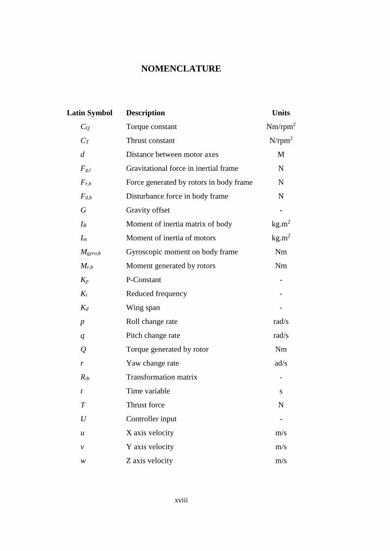
NOMENCLATURE

Latin Symbol Description Units

CQ Torque constant Nm/rpm2

CT Thrust constant N/rpm2

d Distance between motor axes M

Fg,i Gravitational force in inertial frame N

Fr,b Force generated by rotors in body frame N

Fd,b Disturbance force in body frame N

G Gravity offset -

IB Moment of inertia matrix of body kg.m2

Im Moment of inertia of motors kg.m2

Mgyro,b Gyroscopic moment on body frame Nm

Mr,b Moment generated by rotors Nm

Kp P-Constant -

Ki Reduced frequency -

Kd Wing span -

p Roll change rate rad/s

q Pitch change rate rad/s

Q Torque generated by rotor Nm

r Yaw change rate ad/s

Rib Transformation matrix -

t Time variable s

T Thrust force N

U Controller input -

u X axis velocity m/s

v Y axis velocity m/s

w Z axis velocity m/s

xix

x X axis position m

y Y axis position m

z Z axis position m

Greek Symbol Description Units

𝜃 Pitch angle deg

�̇� Pitch rate deg/s

𝜑 Roll angle deg

�̇� Roll rate deg/s

𝜓 Yaw angle deg

�̇� Dynamic viscosity of the fluid deg/s

ω Rotational speed RPM

Abbreviations

2-D Two-Dimensional

3-D Three-Dimensional

IMU Inertial Measurement Unit

PID Proportional Integral Derivative Control

1

CHAPTER 1

1. INTRODUCTION

1.1 Background Information

The quadrotor is a Vertical Takeoff and Landing (VTOL) rotorcraft which is propelled

by four fixed pitch rotor. Because of mechanical simplicity and high mobility, research

related to the quadrotor topic are widespread. The use of area of quadrotors include

military applications such as border patrolling, cartography, cost guards and also

civilian applications such as mapping, search and rescue missions, agricultural

applications, power and nuclear plants inspection etc.

1.2 Present Approach

In recent years, there are a wide range of academic studies related to quadrotor and

quadrotor testbed were done.

One of the first successful quadrotor research platforms is the Stanford Testbed of

Autonomous Rotorcraft for Multi Agent Control (STARMAC) [1]. There are eight

quadrotors currently and the platform is a multi-vehicle test setup to develop and

implement new designs in multi agent control in real world platform. During the

project, two models of quadrotor have been developed namely STARMAC I and

STARMAC II.

2

STARMAC I have a total of 1 kg of thrust and can fly in hover with full throttle about

ten minutes. As IMU, the Microstrain 3DM-G motion sensor was used, including

accelerometer, 3-axis gyroscope and magnetometer. The Trimble Lassen Low Power

GPS module is used for velocity and position measurement [1]. For the additional

measurement of altitude SODAR the Devantech SRFO8 was used. The onboard

sensing and calculations were done in two C programmed Microchip microcontrollers.

The position estimation was done using Extended Kalman Filter (EKF) by combining

GPS and IMU data. The rate of pose estimation is 10 Hz. Attitude control performed

on board is 50 Hz and the communication with ground station was done via a Bluetooth

Class II device over 150 ft. Ground station software was developed in LabView

environment and manual and waypoint track control was done from this software using

laptop. Linear Quadratic Regulator (LQR) technique was used to design attitude loop

control. Also advanced controllers were implemented on STARMAC I such as sliding

mode and reinforcement learning.

On STARMAC II several improvements have been made (Figure 1.1) [2]. The total of

thrust capability has been increased up to 4 kg. The onboard controller has been

divided on two parts. The low level controller was implemented on the Atmega128

microprocessor based board, which controls real-time execution loop and sends

commands to motors. The high level controller and estimation implemented on

embedded Linux based Crossbow Stargate 1.0 single board computer (SBC). This

SBC controller can be replaced by Kubuntu Linux running ADL855 PC104, but due

to the weight it will decrease flight time. The communication with ground station was

replaced with WiFi network instead of Bluetooth communication. Novatel Superstar

II GPS unit with position accuracy 1-2 cm was used for position and velocity

measurement. Also in this platform, for replacing GPS in indoor flights USB camera

was used. Blob tracking software was implemented with 1-2 cm position estimation

accuracy at a rate of 10 Hz. For attitude, altitude and position control Proportional

Integral Derivative (PID) was implemented.

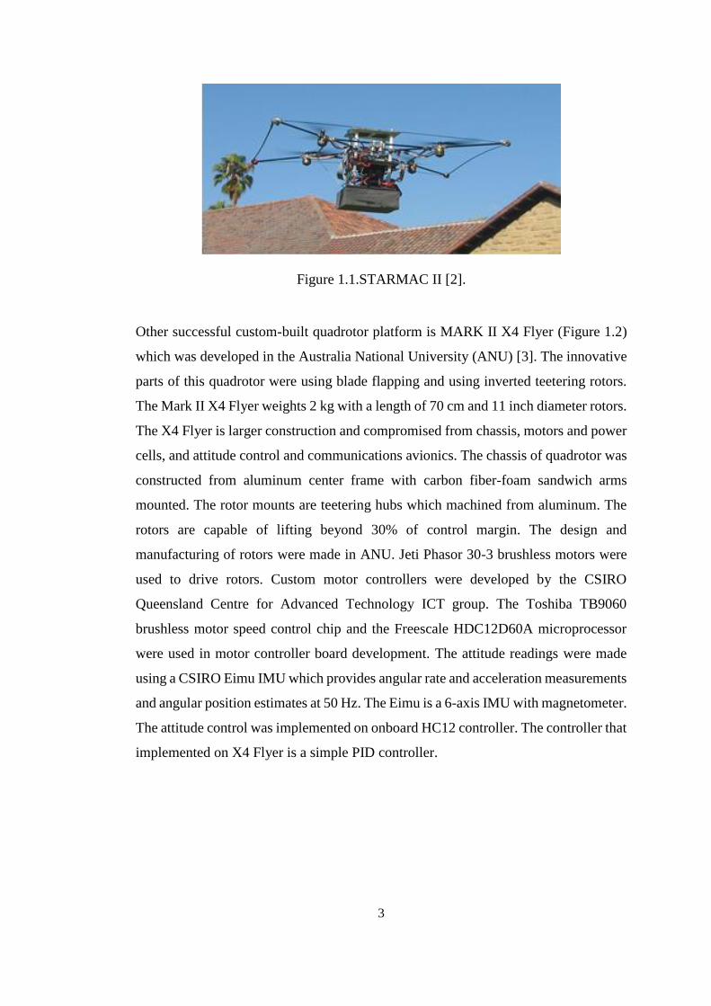
3

Figure 1.1.STARMAC II [2].

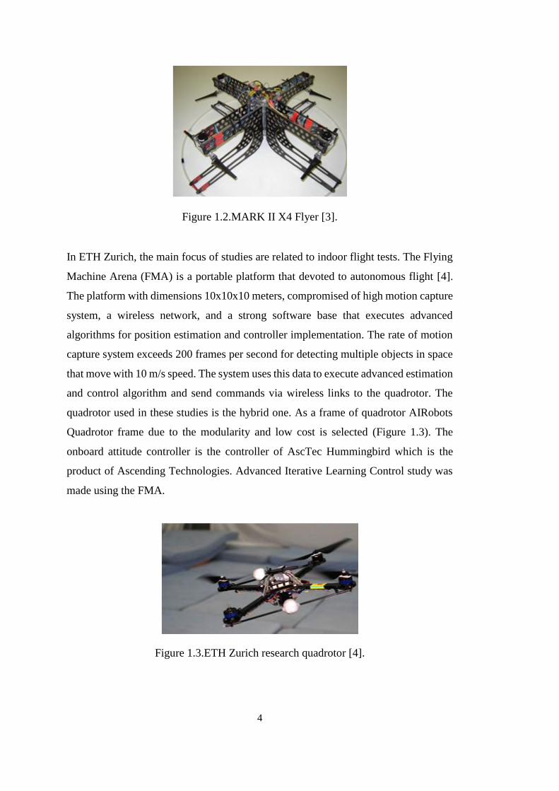
Other successful custom-built quadrotor platform is MARK II X4 Flyer (Figure 1.2)

which was developed in the Australia National University (ANU) [3]. The innovative

parts of this quadrotor were using blade flapping and using inverted teetering rotors.

The Mark II X4 Flyer weights 2 kg with a length of 70 cm and 11 inch diameter rotors.

The X4 Flyer is larger construction and compromised from chassis, motors and power

cells, and attitude control and communications avionics. The chassis of quadrotor was

constructed from aluminum center frame with carbon fiber-foam sandwich arms

mounted. The rotor mounts are teetering hubs which machined from aluminum. The

rotors are capable of lifting beyond 30% of control margin. The design and

manufacturing of rotors were made in ANU. Jeti Phasor 30-3 brushless motors were

used to drive rotors. Custom motor controllers were developed by the CSIRO

Queensland Centre for Advanced Technology ICT group. The Toshiba TB9060

brushless motor speed control chip and the Freescale HDC12D60A microprocessor

were used in motor controller board development. The attitude readings were made

using a CSIRO Eimu IMU which provides angular rate and acceleration measurements

and angular position estimates at 50 Hz. The Eimu is a 6-axis IMU with magnetometer.

The attitude control was implemented on onboard HC12 controller. The controller that

implemented on X4 Flyer is a simple PID controller.

4

Figure 1.2.MARK II X4 Flyer [3].

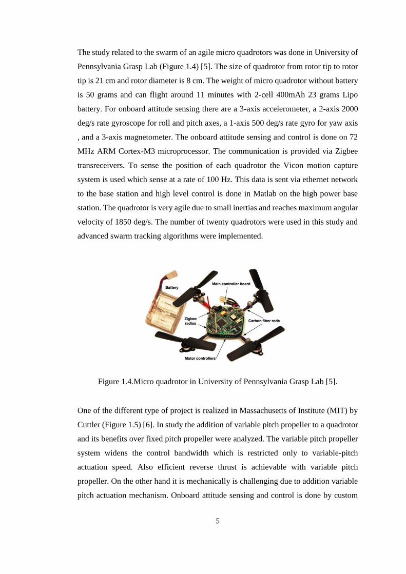
In ETH Zurich, the main focus of studies are related to indoor flight tests. The Flying

Machine Arena (FMA) is a portable platform that devoted to autonomous flight [4].

The platform with dimensions 10x10x10 meters, compromised of high motion capture

system, a wireless network, and a strong software base that executes advanced

algorithms for position estimation and controller implementation. The rate of motion

capture system exceeds 200 frames per second for detecting multiple objects in space

that move with 10 m/s speed. The system uses this data to execute advanced estimation

and control algorithm and send commands via wireless links to the quadrotor. The

quadrotor used in these studies is the hybrid one. As a frame of quadrotor AIRobots

Quadrotor frame due to the modularity and low cost is selected (Figure 1.3). The

onboard attitude controller is the controller of AscTec Hummingbird which is the

product of Ascending Technologies. Advanced Iterative Learning Control study was

made using the FMA.

Figure 1.3.ETH Zurich research quadrotor [4].

5

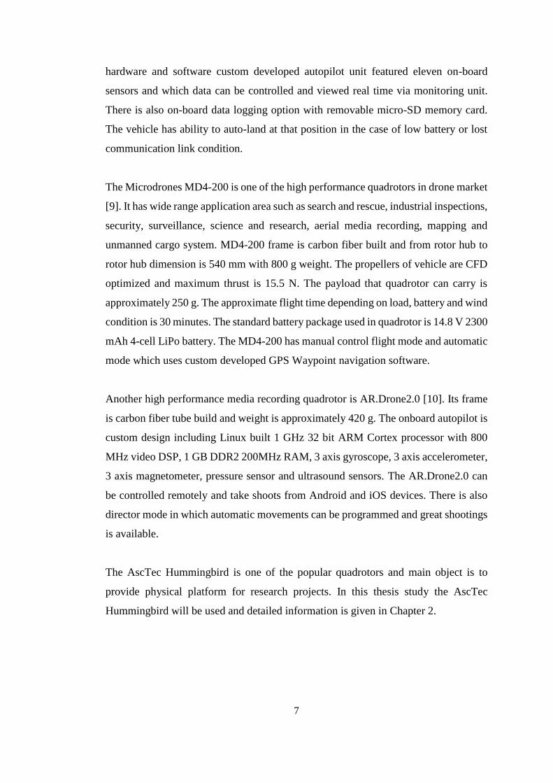
The study related to the swarm of an agile micro quadrotors was done in University of

Pennsylvania Grasp Lab (Figure 1.4) [5]. The size of quadrotor from rotor tip to rotor

tip is 21 cm and rotor diameter is 8 cm. The weight of micro quadrotor without battery

is 50 grams and can flight around 11 minutes with 2-cell 400mAh 23 grams Lipo

battery. For onboard attitude sensing there are a 3-axis accelerometer, a 2-axis 2000

deg/s rate gyroscope for roll and pitch axes, a 1-axis 500 deg/s rate gyro for yaw axis

, and a 3-axis magnetometer. The onboard attitude sensing and control is done on 72

MHz ARM Cortex-M3 microprocessor. The communication is provided via Zigbee

transreceivers. To sense the position of each quadrotor the Vicon motion capture

system is used which sense at a rate of 100 Hz. This data is sent via ethernet network

to the base station and high level control is done in Matlab on the high power base

station. The quadrotor is very agile due to small inertias and reaches maximum angular

velocity of 1850 deg/s. The number of twenty quadrotors were used in this study and

advanced swarm tracking algorithms were implemented.

Figure 1.4.Micro quadrotor in University of Pennsylvania Grasp Lab [5].

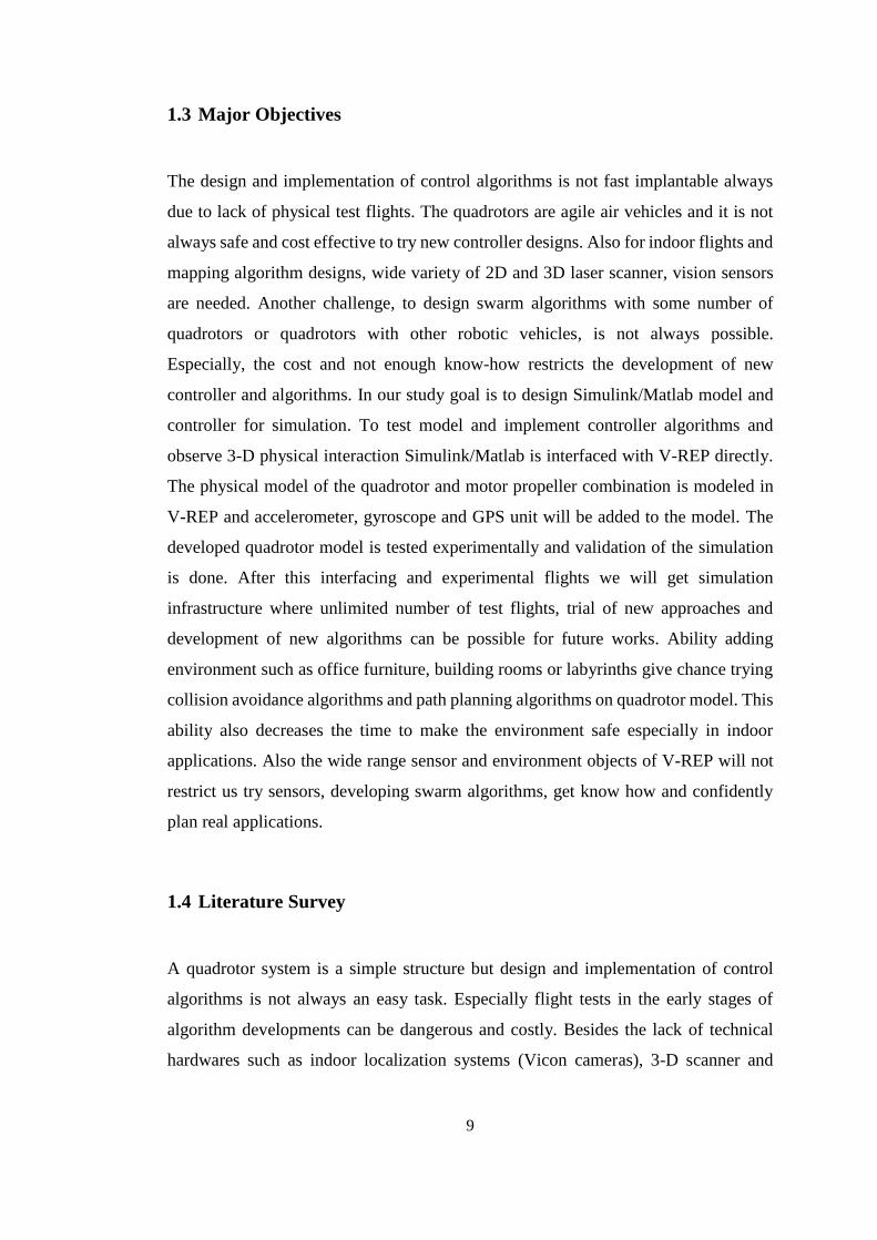
One of the different type of project is realized in Massachusetts of Institute (MIT) by

Cuttler (Figure 1.5) [6]. In study the addition of variable pitch propeller to a quadrotor

and its benefits over fixed pitch propeller were analyzed. The variable pitch propeller

system widens the control bandwidth which is restricted only to variable-pitch

actuation speed. Also efficient reverse thrust is achievable with variable pitch

propeller. On the other hand it is mechanically is challenging due to addition variable

pitch actuation mechanism. Onboard attitude sensing and control is done by custom

6

MIT built controller board. Vicon motion capture system is used for external position

and velocity estimation. A nonlinear quaternion-based controller is implemented on

quadrotor. The control law and trajectory generation algorithms are developed.

Figure 1.5.Variable pitch quadrotor in MIT [6].

There are also commercially available quadrotors in market which generally related to

high performance aerial media recording purpose. One of them is the PHANTOM 4

which is the product of DJI Company [7]. It has manual control flight and position

hold flight modes. Its diagonal size excluding propellers is 350 mm and weight

including battery and propellers is 1380 g. The product includes intelligent flight

battery with 4-cell LiPo which is 5350 mAh 15.2 volts and the device has low voltage

protector. With this battery configuration the maximum time that quadrotor can flight

is approximately 28 minutes. There is also three axis camera stabilization gimbal for

camera recording. The PHANTOM 4 can be controlled and take vision via Android

and iOS devices.

Another market popular quadcopter is Draganflyer X4-P product [8]. This device is

also developed for media recording missions but also can be used for public safety,

industrial inspection and education purposes. The width and length of vehicle is 870

mm and height is 300 mm but it can pack up small and quickly assembled again. The

weight of quadrotor is 1670 g with battery. The frame of quadrotor is patent folding

mostly carbon fiber built design and has excessive weight to strength ratio. It has both

7

hardware and software custom developed autopilot unit featured eleven on-board

sensors and which data can be controlled and viewed real time via monitoring unit.

There is also on-board data logging option with removable micro-SD memory card.

The vehicle has ability to auto-land at that position in the case of low battery or lost

communication link condition.

The Microdrones MD4-200 is one of the high performance quadrotors in drone market

[9]. It has wide range application area such as search and rescue, industrial inspections,

security, surveillance, science and research, aerial media recording, mapping and

unmanned cargo system. MD4-200 frame is carbon fiber built and from rotor hub to

rotor hub dimension is 540 mm with 800 g weight. The propellers of vehicle are CFD

optimized and maximum thrust is 15.5 N. The payload that quadrotor can carry is

approximately 250 g. The approximate flight time depending on load, battery and wind

condition is 30 minutes. The standard battery package used in quadrotor is 14.8 V 2300

mAh 4-cell LiPo battery. The MD4-200 has manual control flight mode and automatic

mode which uses custom developed GPS Waypoint navigation software.

Another high performance media recording quadrotor is AR.Drone2.0 [10]. Its frame

is carbon fiber tube build and weight is approximately 420 g. The onboard autopilot is

custom design including Linux built 1 GHz 32 bit ARM Cortex processor with 800

MHz video DSP, 1 GB DDR2 200MHz RAM, 3 axis gyroscope, 3 axis accelerometer,

3 axis magnetometer, pressure sensor and ultrasound sensors. The AR.Drone2.0 can

be controlled remotely and take shoots from Android and iOS devices. There is also

director mode in which automatic movements can be programmed and great shootings

is available.

The AscTec Hummingbird is one of the popular quadrotors and main object is to

provide physical platform for research projects. In this thesis study the AscTec

Hummingbird will be used and detailed information is given in Chapter 2.

8

(a) PHANTOM 4 [7]

(b) Draganflyer X4-P [8]

(c) Microdrones MD4-200 [9]

(d) AR.Drone2.0 [10]

Figure 1.6. Some popular commercial quadrotors in market

9

1.3 Major Objectives

The design and implementation of control algorithms is not fast implantable always

due to lack of physical test flights. The quadrotors are agile air vehicles and it is not

always safe and cost effective to try new controller designs. Also for indoor flights and

mapping algorithm designs, wide variety of 2D and 3D laser scanner, vision sensors

are needed. Another challenge, to design swarm algorithms with some number of

quadrotors or quadrotors with other robotic vehicles, is not always possible.

Especially, the cost and not enough know-how restricts the development of new

controller and algorithms. In our study goal is to design Simulink/Matlab model and

controller for simulation. To test model and implement controller algorithms and

observe 3-D physical interaction Simulink/Matlab is interfaced with V-REP directly.

The physical model of the quadrotor and motor propeller combination is modeled in

V-REP and accelerometer, gyroscope and GPS unit will be added to the model. The

developed quadrotor model is tested experimentally and validation of the simulation

is done. After this interfacing and experimental flights we will get simulation

infrastructure where unlimited number of test flights, trial of new approaches and

development of new algorithms can be possible for future works. Ability adding

environment such as office furniture, building rooms or labyrinths give chance trying

collision avoidance algorithms and path planning algorithms on quadrotor model. This

ability also decreases the time to make the environment safe especially in indoor

applications. Also the wide range sensor and environment objects of V-REP will not

restrict us try sensors, developing swarm algorithms, get know how and confidently

plan real applications.

1.4 Literature Survey

A quadrotor system is a simple structure but design and implementation of control

algorithms is not always an easy task. Especially flight tests in the early stages of

algorithm developments can be dangerous and costly. Besides the lack of technical

hardwares such as indoor localization systems (Vicon cameras), 3-D scanner and

10

visual sensors etc. are reducing development ability. Another challenge the studies

related to swarm flight algorithms requires number of quadrotors and technological

infrastructure. Also especially in indoor applications the safety of environment is

important and pillow, netting etc. safety precautions is needed in real flights. To avoid

these types of problems simulator platform tests and implementations have been

spread. Most of these simulator studies are generally developed in Matlab/Simulink

platform. In his thesis Martinez modelled the quadrotor in Matlab/Simulink platform

and his model based around Draganfly XPro quadrotor [11]. The model included

detailed DC motor model and rotor model based on Blade Element Theory verified by

wind tunnel experiments, equation of motions of quadrotor based on Newton-Euler

formulation, horizontal and vertical gusts, and possible asymmetries due to motor

property or rotor weight. The model simulations ran in variable-step solvers. In this

thesis, the scope of the work is done according to the open loop flight dynamics of the

quadrotor and no controller was implemented. The non-linear model of quadrotor was

derived using classical mechanics and multiple control techniques such as PID, LQ

and robust control techniques H∞ and µ with DK-iteration were employed in

Matlab/Simulink in Marcelo’s thesis study [12]. The quadrotor parameters like inertia,

aerodynamic drag coefficient and thrust coefficient were validated experimentally.

Karwoski developed a model in Simulink based on AscTec Hummingbird quadrotor

for design and analysis of variable control systems [13]. In his work, he built

experimental safe area for the flight tests of quadrotor as shown in Figure 1.7.

11

(a) Flying area with pillows and net (b) Quadrotor after hitting net

Figure 1.7. Flight test area built for AscTec Hummingbird experiments [13].

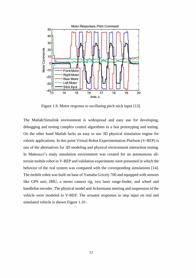
Then non-linear dynamic model was derived and implemented in Simulink/Matlab

platform and PID controller was designed by step-step starting form P-controller, then

trying PD, PI and PID controllers in simulation environment. There were made

experimental flights that measured quadrotor attitude loop response to remote stick

input. Also motor command responses to roll and pitch stick input were also logged

and analyzed as shown in Figure 1.8 and Figure 1.9 .

Figure 1.8. Motor response to oscillating roll stick input [13].

12

Figure 1.9. Motor response to oscillating pitch stick input [13].

The Matlab/Simulink environment is widespread and easy use for developing,

debugging and testing complex control algorithms in a fast prototyping and testing.

On the other hand Matlab lacks an easy to use 3D physical simulation engine for

robotic applications. In this point Virtual Robot Experimentation Platform (V-REP) is

one of the alternatives for 3D modeling and physical environment interaction testing.

In Matteucci’s study simulation environment was created for an autonomous all-

terrain mobile robot in V-REP and validation experiments were presented in which the

behavior of the real system was compared with the corresponding simulations [14].

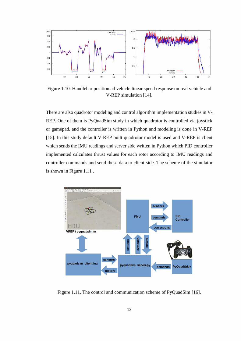
The mobile robot was built on base of Yamaha Grizzly 700 and equipped with sensors

like GPS unit, IMU, a stereo camera rig, two laser range-finder, and wheel and

handlebar encoder. The physical model and Ackermann steering and suspension of the

vehicle were modeled in V-REP. The actuator responses to step input on real and

simulated vehicle is shown Figure 1.10 .

13

Figure 1.10. Handlebar position ad vehicle linear speed response on real vehicle and

V-REP simulation [14].

There are also quadrotor modeling and control algorithm implementation studies in V-

REP. One of them is PyQuadSim study in which quadrotor is controlled via joystick

or gamepad, and the controller is written in Python and modeling is done in V-REP

[15]. In this study default V-REP built quadrotor model is used and V-REP is client

which sends the IMU readings and server side written in Python which PID controller

implemented calculates thrust values for each rotor according to IMU readings and

controller commands and send these data to client side. The scheme of the simulator

is shown in Figure 1.11 .

Figure 1.11. The control and communication scheme of PyQuadSim [16].

14

In Riccardo’s study the interface of Matlab/Simulink with V-REP using ROS as

communication middleware is done and the default V-REP quadrotor model control is

done using visual servoing [17]. In this project the camera and quadrotor module of

V-REP is used where images sent from V-REP to ROS node and processed using ViSP

library. The tracked location data from ROS node is sent to Simulink and calculated

thrust commands for each motor are sent back to V-REP. The software diagram is

shown in Figure 1.12.

The configuration of V-REP and ROS to work in parallel, using ROS packages for

pose estimation based on vision and for the design and use fuzzy logic control system

in quadrotor is done in Mendez’s study [18]. The experimental flights were set by a

real Ar.Drone parrot power edition quadrotor and the results support virtual flight test

data. As a conclusion of study three ROS packages were built which the first one is

control part related to fuzzy logic controller, the second one is to process image and

extract information from them in real world and simulation, and the third one is to link

image process information to the controller in real world and simulation platform. The

response of three axis fuzzy logic controllers to step signal input in simulation is shown

in Figure 1.13 and the response of three controllers against disturbances in real life is


Figure 1.12. The V-REP, ROS and Simulink software flow diagram [17].

15

Figure 1.13. Response of three axis fuzzy logic controller working together to step

input in simulation [18].

Figure 1.14. Response of three axis fuzzy logic controller against disturbances in real

[18].

1.5 Outline of the Thesis

This study is comprised of six chapters to explain the scope of the thesis. In Chapter

1, brief background information is given, and then present approach related quadrotors

is described. After mentioning objectives of work, the literature survey related to

subject is presented. Chapter 2 describes the hardware and software toolkit properties

16

of quadrotor that will be used in this thesis. In Chapter 3, the mathematical model of

quadrotor is derived and classical PID controller is designed. The first section of

Chapter 4 describes the capabilities of V-REP, and then in related sections modeling

of propeller and quadrotor in V-REP, Simulink/Matlab interfacing with V-REP are

presented. Thereafter, some case simulation results are given in first section of Chapter

5. Then experimental setups and controller implementation on real quadrotor are

described in the next sections of Chapter 5. In fourth section of Chapter 5 experimental

and simulation data comparison is given. In final part of Chapter 5, the collision

avoidance and wall following studies is presented to demonstrate the simulation

infrastructure capabilities. Chapter 6 covers the general conclusion and future

recommendations for the study.

17

CHAPTER 2

2. QUADROTOR SETUP

2.1 Quadrotor Properties

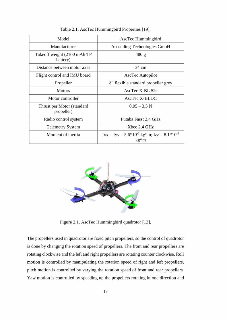
The quadrotor that is used in this study is an AscTec Hummingbird (Figure 2.1) which

is equipped with the AscTec Autopilot [19]. The quadrotor, shown in Figure 2.1 is

small, lightweight and an ideal platform for testing flights in indoor environments. The

main frame of quadrotor is made out of sandwich material consisting of carbon fiber

and balsa wood. Due to lightweight and small size control bandwidth does not restrict

aggressive maneuvers significantly. The system has a pressure sensor, three axis

compass, GPS unit, an acceleration sensor, and three gyroscopes (one for each axis).

AscTec Autopilot main board consist of two ARM 7 60MHz, 32 Bit microcontrollers

– a low level processor (LLP) and a high level processor (HLP). LLP collects IMU

(accelerometer + gyroscopes) data, sends commands to the motor controller and is

responsible from attitude control of quadrotor. The HLP controls the GPS and is free

for user defined control algorithm designs. The control algorithms can be designed in

Simulink/Matlab environment, the control system is then translated to the C code by

the Real Time Workshop Embedded coder. The AscTec HL-SDK provides all

necessary tools to program custom C code and to flash and debug the code on the

processor. The communication of AscTec Hummingbird with ground is provided by a

wireless Xbee model via serial port. The technical details of the quadrotor are

summarized in Table 2.1.

18

Table 2.1. AscTec Hummingbird Properties [19].

Model AscTec Hummingbird

Manufacturer Ascending Technologies GmbH

Takeoff weight (2100 mAh TP

battery)

480 g

Distance between motor axes 34 cm

Flight control and IMU board AscTec Autopilot

Propeller 8” flexible standard propeller grey

Motors AscTec X-BL 52s

Motor controller AscTec X-BLDC

Thrust per Motor (standard

propeller)

0,05 – 3,5 N

Radio control system Futaba Fasst 2,4 GHz

Telemetry System Xbee 2,4 GHz

Moment of inertia Ixx = Iyy = 5.6*10-3 kg*m; Izz = 8.1*10-3

kg*m

Figure 2.1. AscTec Hummingbird quadrotor [13].

The propellers used in quadrotor are fixed pitch propellers, so the control of quadrotor

is done by changing the rotation speed of propellers. The front and rear propellers are

rotating clockwise and the left and right propellers are rotating counter clockwise. Roll

motion is controlled by manipulating the rotation speed of right and left propellers,

pitch motion is controlled by varying the rotation speed of front and rear propellers.

Yaw motion is controlled by speeding up the propellers rotating in one direction and

19

slowing down ones spinning in other direction. So the trust does not change, but

change of angular momentum causes rotation in yaw axis.

2.2 AscTec Simulink Toolkit Overview and Connections

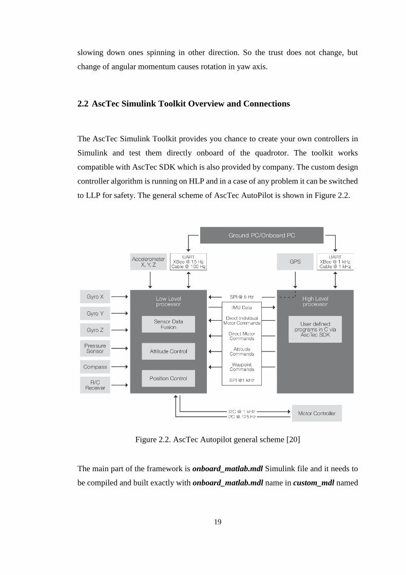
The AscTec Simulink Toolkit provides you chance to create your own controllers in

Simulink and test them directly onboard of the quadrotor. The toolkit works

compatible with AscTec SDK which is also provided by company. The custom design

controller algorithm is running on HLP and in a case of any problem it can be switched

to LLP for safety. The general scheme of AscTec AutoPilot is shown in Figure 2.2.

Figure 2.2. AscTec Autopilot general scheme [20]

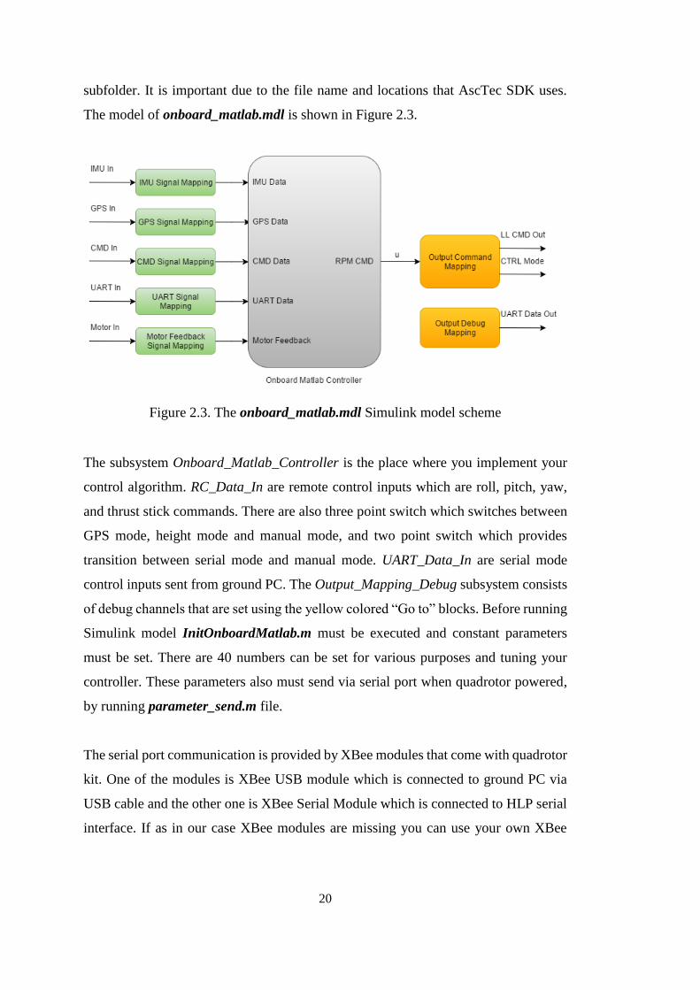
The main part of the framework is onboard_matlab.mdl Simulink file and it needs to

be compiled and built exactly with onboard_matlab.mdl name in custom_mdl named

20

subfolder. It is important due to the file name and locations that AscTec SDK uses.

The model of onboard_matlab.mdl is shown in Figure 2.3.

Figure 2.3. The onboard_matlab.mdl Simulink model scheme

The subsystem Onboard_Matlab_Controller is the place where you implement your

control algorithm. RC_Data_In are remote control inputs which are roll, pitch, yaw,

and thrust stick commands. There are also three point switch which switches between

GPS mode, height mode and manual mode, and two point switch which provides

transition between serial mode and manual mode. UART_Data_In are serial mode

control inputs sent from ground PC. The Output_Mapping_Debug subsystem consists

of debug channels that are set using the yellow colored “Go to” blocks. Before running

Simulink model InitOnboardMatlab.m must be executed and constant parameters

must be set. There are 40 numbers can be set for various purposes and tuning your

controller. These parameters also must send via serial port when quadrotor powered,

by running parameter_send.m file.

The serial port communication is provided by XBee modules that come with quadrotor

kit. One of the modules is XBee USB module which is connected to ground PC via

USB cable and the other one is XBee Serial Module which is connected to HLP serial

interface. If as in our case XBee modules are missing you can use your own XBee

21

modules and configure pairs by XCTU Tool software. The communication baud rate

is 57600 (Data Bits: 8, Parity: None, Stop Bits: 1, Flow Control: None).

To communicate with ground PC in real time UART_Communication.mdl Simulink

model must be executed. There are sixty debug channels under

Debug_Mapping_Extended mask and each channel gets the values that assigned in

onboard_matlab.mdl. Also CPU load and battery voltage can be displayed

continuously through display. There are twelve control channels to send data from

ground PC to quadrotor and this channel values can be constants and as well as control

signals. The UART_Communication.mdl debug channel mappings and control inputs

can be seen in Figure 2.4. Debug_Scopes subsystem is area where received data is

visualized and collected.

Figure 2.4. UART_Communication.mdl Simulink model scheme

After building your onboard_matlab.mdl Simulink model using Simulink Code

Generation C-code must be generated and stored to onboard_matlab_ert_rtw. Then

asctec-sdk2.0.zip package must be installed which comes with AscTec SDK. This

package installs Eclipse, ARM-GCC, OpenOCD and JTAG drivers on your system.

22

AutoPilot_HL-Simulink_SDK_v2.0 project must be imported to the working

workspace directory in AscTec Eclipse and built. Afterwards JTAG adapter must be

connected to quadrotor and OpenOCD AscTec-JTAG must be selected as run option

and code is uploaded to quadrotor HLP. After restarting quadrotor custom built

controller code is running on quadrotor HLP onboard.

23

CHAPTER 3

3. MATHEMATICAL MODEL AND CONTROLLER DESIGN

3.1 Mathematical Model of Quadrotor

The quadrotor that we use in our study is fixed pitch propeller quadrotor. The angle of

attack of fixed pitch propeller is constant and thrust force produced by propeller is

adjusted by changing the rotational speed of corresponding rotor. The relation between

thrust and rotational speed is as follows,

𝑇 = 𝑐𝑇𝜔2 (3.1)

where 𝑐𝑇 is motor-prop specified thrust constant that depends on used propeller model.

The relation between propeller torque and rotational speed is as follows,

𝑄 = 𝑐𝑄𝜔2 (3.2)

Figure 3.1.Free body diagram of quadrotor [21]

The control of quadrotor model is done by adjusting rotational speed of each propeller.

Thus the four controller inputs for quadrotor control are as follows:

24

𝑈1 = 𝑇1 + 𝑇2 + 𝑇3 + 𝑇4 (3.3)

𝑈2 = 𝑇4 − 𝑇2 (3.4)

𝑈3 = 𝑇3 − 𝑇1 (3.5)

𝑈4 = 𝑄2 + 𝑄4 − 𝑄1 − 𝑄3 (3.6)

As it can be seen from equation (3.3) 𝑈1 input is related to the z direction motion of

the quadrotor and is equal to the sum of all thrust forces generated by four rotors. To

realize x and y direction motion of the quadrotor is done by changing roll and pitch

angles via adjusting orientation of 𝑈1. It is seen that roll motion of quadrotor is directly

related to the 𝑈2 input which is the thrust value difference between the right and left

rotor (3.4). In similar way the pitch motion is achieved with the thrust value difference

between the front and rear rotor which is defined in equation (3.5) as 𝑈3 input. The

units of 𝑈1, 𝑈2 and 𝑈3are N, where the unit of 𝑈4is Nm. The input 𝑈4 is related to the

yaw motion of the quadrotor, which is torque value difference between the sum of

right and left rotor torque values and the sum of front and rear rotor torque values (3.6).

It must be noticed that the front and rear rotors rotate clockwise, while right and left

rotors rotate counterclockwise.

The matrix describing the thrusts and torques is shown below (3.7):

[

Σ𝑇𝜏𝜙

𝜏𝜃

𝜏𝜓

] = [

𝑐𝑇 𝑐𝑇 𝑐𝑇 𝑐𝑇

0 𝑑𝑐𝑇 0 −𝑑𝑐𝑇

−𝑑𝑐𝑇 0 𝑑𝑐𝑇 0−𝑐𝑄 𝑐𝑄 −𝑐𝑄 𝑐𝑄

]

[ 𝜔1

2

𝜔22

𝜔32

𝜔42]

(3.7)

, where 𝑑 is the distance between the propeller rotation axes.

Afterwards in this section the effect of external forces and moments acting on the

quadrotor body is defined. For simplicity some of the forces and moments are ignored.

The first important force acting on the center of gravitation (CG) of a quadrotor body

is due to gravitation with constant gravitational acceleration 𝑔 = 9.81 𝑚 𝑠2⁄ . The

expression of gravity force in inertial frame is shown as follows (3.8)

25

𝐹𝑔,𝑖 = −𝑚 [

00𝑔]

(3.8)

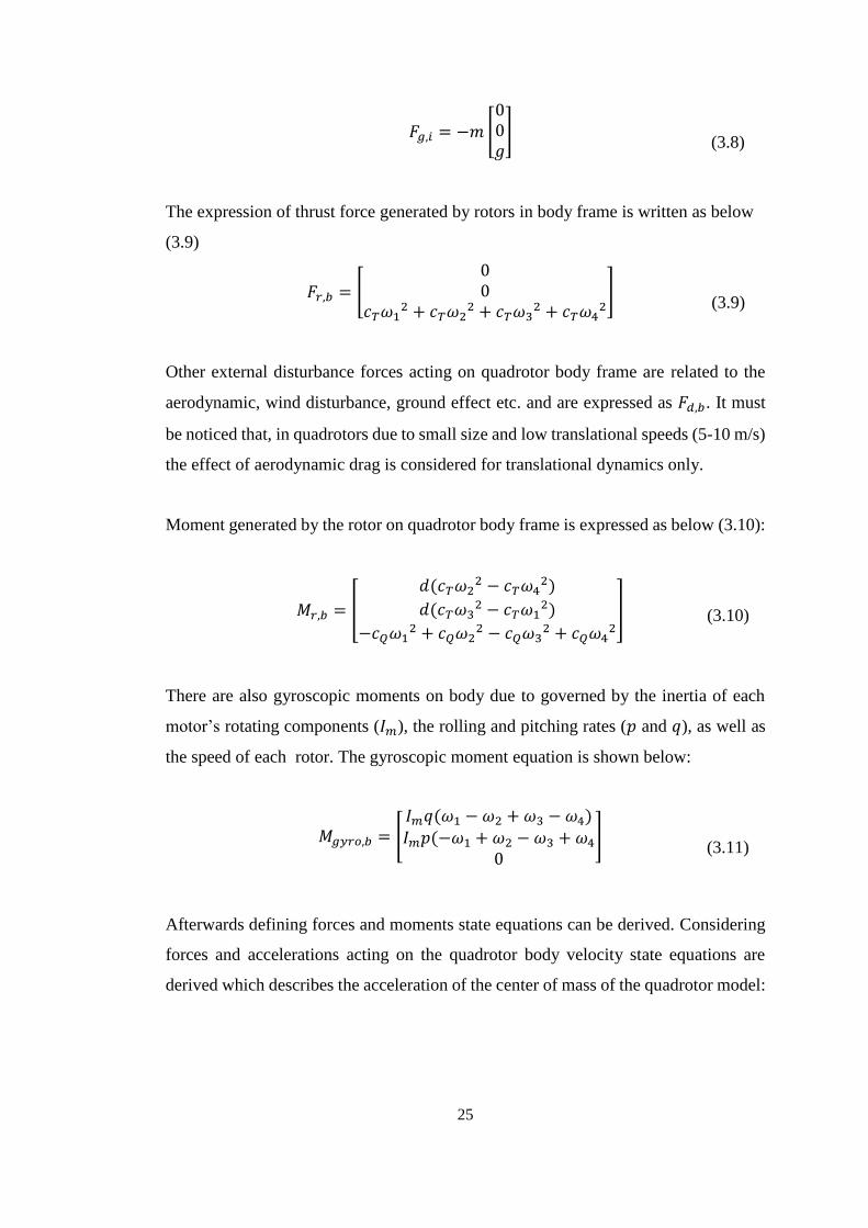
The expression of thrust force generated by rotors in body frame is written as below

(3.9)

𝐹𝑟,𝑏 = [

00

𝑐𝑇𝜔12 + 𝑐𝑇𝜔2

2 + 𝑐𝑇𝜔32 + 𝑐𝑇𝜔4

2]

(3.9)

Other external disturbance forces acting on quadrotor body frame are related to the

aerodynamic, wind disturbance, ground effect etc. and are expressed as 𝐹𝑑,𝑏. It must

be noticed that, in quadrotors due to small size and low translational speeds (5-10 m/s)

the effect of aerodynamic drag is considered for translational dynamics only.

Moment generated by the rotor on quadrotor body frame is expressed as below (3.10):

𝑀𝑟,𝑏 = [

𝑑(𝑐𝑇𝜔22 − 𝑐𝑇𝜔4

2)

𝑑(𝑐𝑇𝜔32 − 𝑐𝑇𝜔1

2)

−𝑐𝑄𝜔12 + 𝑐𝑄𝜔2

2 − 𝑐𝑄𝜔32 + 𝑐𝑄𝜔4

2

]

(3.10)

There are also gyroscopic moments on body due to governed by the inertia of each

motor’s rotating components (𝐼𝑚), the rolling and pitching rates (𝑝 and 𝑞), as well as

the speed of each rotor. The gyroscopic moment equation is shown below:

𝑀𝑔𝑦𝑟𝑜,𝑏 = [

𝐼𝑚𝑞(𝜔1 − 𝜔2 + 𝜔3 − 𝜔4)𝐼𝑚𝑝(−𝜔1 + 𝜔2 − 𝜔3 + 𝜔4

0

]

(3.11)

Afterwards defining forces and moments state equations can be derived. Considering

forces and accelerations acting on the quadrotor body velocity state equations are

derived which describes the acceleration of the center of mass of the quadrotor model:

26

[�̇��̇��̇�

] = 𝐹𝑟,𝑏 − 𝐹𝑑,𝑏 + 𝐹𝑔,𝑏 − Ω [𝑢𝑣𝑤

] (3.12) where 𝐹𝑔,𝑏 = 𝑅𝑏𝑖𝐹𝑔,𝑖 (3.13) and

Ω = [

0 −𝑟 𝑞𝑟 0 −𝑝

−𝑞 𝑝 0]

(3.14)

It must be noticed that 𝑅𝑏𝑖 is rotation matrix to translate the translational velocity of

quadrotor in the components of body fixed frame and inertial frame (3.15). The

sequence of rotations of according to the aerospace rotation sequence is in order of

yaw, pitch, and roll rotation. 𝑅𝑖𝑏 is the transpose of 𝑅𝑏𝑖 matrix.

𝑅𝑏𝑖 = [

c(𝜃) c(𝜓) c(𝜃) s(𝜓) −s(𝜃)

(− c(𝜙) s(𝜓) + s(𝜙) s(𝜃) c(𝜓)) (𝑐(𝜙)𝑐(𝜓) + 𝑠(𝜙)𝑠(𝜃)𝑠(𝜓)) s(𝜙) c(𝜃)

(𝑠(𝜙)𝑠(𝜓) + 𝑐(𝜙)𝑠(𝜃)𝑐(𝜓)) (−𝑠(𝜙)𝑐(𝜓) + 𝑐(𝜙)𝑠(𝜃)𝑠(𝜓)) c(𝜙) c(𝜃)]

(3.15)

Next position state equation is derived which describes the linear velocity of the center

of mass of the quadrotor in the inertial frame.

[�̇��̇��̇�] = 𝑅𝑖𝑏 [

𝑢𝑣𝑤

]

(3.16)

Then angular velocity state equations are derived, which describe the change in roll,

pitch, and yaw rates of the quadrotor by taking into account the inertia, angular

velocity, and the moments applied by the rotors.

[�̇��̇��̇�

] = (𝐼𝐵)−1 [𝑀𝑟,𝑏 + 𝑀𝑔𝑦𝑟𝑜,𝑏 − Ω𝐼𝐵 [𝑝𝑞𝑟]]

(3.17)

where 𝐼𝐵 is inertia matrix. Next the rate of change of the Euler angles is determined in

the inertial frame by multiplying quadrotor body angular rate changes by angular

velocity transformation matrix:

27

[

�̇�

�̇��̇�

] = [

1 𝑡(𝜃) 𝑠(𝜙) 𝑡(𝜃) 𝑐(𝜙)

0 𝑐(𝜙) −𝑠(𝜙)

0 𝑠(𝜙) /𝑐(𝜃) 𝑐(𝜙)/ 𝑐(𝜃)] [

𝑝𝑞𝑟]

(3.18)

It must be noticed that there is a singularity at 𝜃 = ±90° in (3.18).

3.2 PID Controller Design

Classical PID control is selected as the control method and in this section the basic

theory of this controller is described.

The PID controller is composed of three components: Proportional, Integral and

Derivative part. The proportional control reduces the rise time and there is always

steady state error offset in response to a step input. Adding integral reduces the steady

state error but may cause oscillatory response of slowly decreasing amplitude. Due to

integrator windup there can be instability in controller, so saturation limits must be

applied to the integrator. Adding only derivative control to proportional control

improves the transient response and reduces overshoot of response to the step input.

So the derivative control increases the stability of controller. There is no direct effect

of derivative controller to the steady state error, but as it acts like damper, large

proportional gains can be selected for decreasing the steady state error. Adding both

integral and derivative controller to proportional controller results in PID controller,

which reduces rise time, maximum overshoot and removes steady state error.

The tuning process is one of the challenging parts of PID controller. There are several

tuning algorithms such as Ziegler-Nichols and Lambda tuning. In our study we used

iterative hand tuning according to response analyzes.

Using this mathematical model PID controller is designed for the altitude and attitude

control of the quadrotor. The hovering height and roll, pitch, and yaw angles have been

controlled.

28

The yaw control is not so critical control among the quadrotor controls because it has

no direct effect on the quadrotor’s motion. The effect of disturbances on the yaw is

relatively small, so there is no need to large controller gains. Also bandwidth of

controller is also small. The control scheme of the controller is as below in Figure 3.2.

Figure 3.2.Yaw PID controller scheme

The roll and pitch controllers are same due to the quadrotor’s symmetrical layout. Due

to this, there is direct relationship with x and y direction acceleration the control

bandwidth of controllers is higher relative to the yaw control. The controller schemes

are in Figure 3.3 and Figure 3.4.

Figure 3.3.Roll PID controller scheme

29

Figure 3.4.Pitch PID Controller scheme

In hover condition, above the ground effect, the control output is nearly proportional

to the z axis acceleration on quadrotor body frame. To keep the hover altitude a large

number of gravity offset (G) is required to defeat the gravity force. PID controller is

needed to stabilize the altitude motion. The control scheme is described in Figure 3.5.

𝐺 =

𝑧𝑐𝑚𝑑 + 𝑚𝑔

cos𝜑 sin 𝜃

(3.19)

Figure 3.5.Altitude PID controller

31

CHAPTER 4

4. V-REP MODEL AND MATLAB/SIMULINK INTERFACING

4.1 Virtual Robot Experimentation Platform (V-REP)

In our study, we have used the Virtual Robot Experimentation Platform (V-REP), a

physical simulator which provides an easy and intuitive environment to create your

own virtual platform and to include some popular robots, objects, structures, actuators

and sensors.

Virtual Robot Experimental Platform (V-REP) is the product of Coppelia Robotics

that developed for general purpose robot simulation. Customized user interface and a

modular structure integrated development environment are the main characteristics of

the simulator. Modularity is in high level both for the simulation objects and control

methods. The easy use of development environment inside the simulator provides the

creation of robots and simulation cases. This capability permits for fast prototyping,

algorithm design and implementation. During the active simulation this area acts as

real 3D world and gives real time feedback according to the behavior of models. The

objects that compose the scene, the control mechanism and the computing modules are

the three main functionalities of the simulator. The following object types compose

the V-REP simulation scene or model:

Shapes: Shapes are triangular faced rigid mesh objects. These objects can be

used in collision detections against other collidable objects and minimum

distance calculations with other measurable objects. Shapes also can be

32

detected by proximity and vision sensors. Another property of shapes is that

can be cut by mils.

Joints: Joints are the tools used for building mechanisms and moving object,

which has at least one Degree of Freedom (DOF). There are four types joints

which are revolute, prismatic, and spherical and screw joints. The operation

modes of joints are passive mode, inverse kinematic mode, dependent mode,

motion mode and finally torque or force mode. Dynamic model of actuator can

be modeled enabling torque or force mode which also has position control

(PID) method.

Proximity sensors: From ultrasonic to infrared nearly all type of proximity

sensors can be modeled to simulate proximity sensors. They do an exact

distance calculation between their sensing point and any detectable entity that

interferes with its detection volume.

Vision sensors: They will render all renderable objects in simulation scene

(colors, objects sizes, depth maps, etc.) and extract complex image

information. A built-in filter and image processing functions ease the use of

vision sensors in simulation.

Force sensors: Force sensor are objects that measures transmitted force and

torque values between two or more objects. The force sensor working principle

can be modeled as real one, so that they can even be broken in overshot force

and torque values.

Graphs: Graphs are objects for to record, visualize and export data from a

simulation. The graphs feature in V-REP are very powerful, so that time

graphs, x/y graphs and 3D graphs can be generated for data types applied to

specific objects to record.

Cameras: Cameras are objects that you can monitor your simulation from

different viewpoints. You can either add multi view windows in one view

window or attach each view to separate windows.

Lights: Lights are the objects that light the simulation scene and directly

influence camera and vision sensors.

Paths: Paths are objects that define a rotational, translational or combined path

or trajectory in space.

33

Dummies: A dummy is a type of object that can be defined as a reference frame

or point of orientation attached to the object. They are useful especially for

path-trajectory planning and following. Dummies are generally multipurpose

helper object in combination with other objects. It must be noticed that alone

they are not so useful.

Mills: Using mills almost any type of cutting volumes as long as they are

convex can be modeled. Mills always have a convex cutting volume; however

they can be combined to generate a non-convex cutting volume or more

complex volumes.

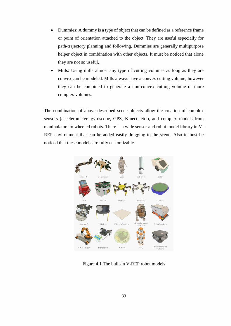
The combination of above described scene objects allow the creation of complex

sensors (accelerometer, gyroscope, GPS, Kinect, etc.), and complex models from

manipulators to wheeled robots. There is a wide sensor and robot model library in V-

REP environment that can be added easily dragging to the scene. Also it must be

noticed that these models are fully customizable.

Figure 4.1.The built-in V-REP robot models

34

There are various control mechanisms to manage the behavior of each simulation

objects. These controllers can be implemented not only inside of the simulation

environment and also outside of the simulation environment. The main internal control

mechanism is the use of child scripts, which can be associated with any element in the

scene. The child scripts handle a particular part of the simulation and they are an

integral part of their associated object. Due to that property they can be duplicated and

serialized, together with them. Therefore, they are a single package containing the

model parameters together with its control which makes them portable and scalable.

Child scripts have two execution modes. Non-threaded child scripts are pass-through

scripts which means every time they are called they execute some task and then return

to control. Threaded child scripts launches in thread and is handled by main script

code. Threaded child scripts require more advanced programming knowledge

compared ton on-threaded child scripts. Also threaded child scripts can waste more

processing power and time than non-threaded ones, and there some lag can be observed

in response to a simulation commands. The main script handles both threaded and non-

threaded child scripts. These embedded scripts open and handle communication lines

start remote API servers, launch executables, load and unload plugins, and can register

ROS publishers and subscribers.

For simulator-in-the-loop configuration tests V-REP offers also a method to control

the simulation from outside the simulator by external implied controller algorithm. The

controller developed in remote API interface in V-REP communicates with the

simulation scene using a socket communication. It is composed by remote API server

services and remote API clients. The client side can be developed in C/C++, Python,

Java, Matlab or Urbi languages, also embedded in any software running on remote

control hardware or real robots, and it allows remote function calling, as well as fast

data streaming. Functions support two calling methods to adapt to any configuration:

blocking, waiting until the server replies, or non-blocking, reading streamed

commands from a buffer. The schematic of this communication mode is shown in

Figure 4.2. Plugins implement the API server inside V-REP for providing a simulation

process with standard LUA commands. So they generally are used in combination with

scripts. On the other hand, if there is need for either fast calculation case (compiled

35

languages most of the time are faster than scripts) or an interface to a real device (e.g.

real robot), plugins provide special functionality.

(a)

(b)

Figure 4.2.The remote API communication modes: (a) blocking function call, (b)

non-blocking function call [22].

The interaction between objects in the simulation scene is calculated by various

calculation modes. V-REP's dynamics module currently supports four different

physics engines: the Bullet physics library [23], the Open Dynamics Engine [24], the

Vortex Dynamics engine [25] and the Newton Dynamics engine [26]. At any time, it

is easy to switch from one engine to the other quickly according to the simulation

needs. The reason for this diversity in physics engine support is that physics simulation

36

is a complex task which can be achieved with various degrees of precision, speed, or

with support of diverse features.

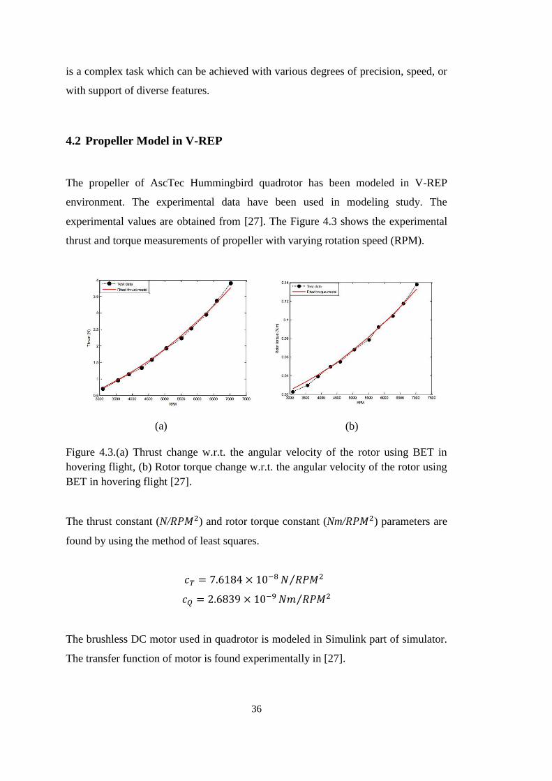
4.2 Propeller Model in V-REP

The propeller of AscTec Hummingbird quadrotor has been modeled in V-REP

environment. The experimental data have been used in modeling study. The

experimental values are obtained from [27]. The Figure 4.3 shows the experimental

thrust and torque measurements of propeller with varying rotation speed (RPM).

(a)

(b)

Figure 4.3.(a) Thrust change w.r.t. the angular velocity of the rotor using BET in

hovering flight, (b) Rotor torque change w.r.t. the angular velocity of the rotor using

BET in hovering flight [27].

The thrust constant (N/𝑅𝑃𝑀2) and rotor torque constant (Nm/𝑅𝑃𝑀2) parameters are

found by using the method of least squares.

𝑐𝑇 = 7.6184 × 10−8 𝑁 𝑅𝑃𝑀2⁄

𝑐𝑄 = 2.6839 × 10−9 𝑁𝑚 𝑅𝑃𝑀2⁄

The brushless DC motor used in quadrotor is modeled in Simulink part of simulator.

The transfer function of motor is found experimentally in [27].

37

𝐺𝑠 =3.5

0.0044𝑠2 + 0.08𝑠 + 1

The estimated parameter then has been implemented in V-REP environment. The CAD

model of propeller is imported to the platform and appropriate LUA embedded script

has been written which gets the rotation speed and particle velocity from main script.

Particle velocity is modeled for ground disturbance studies in future studies. In Figure

4.4 there is one example work of propeller at 3900 RPM which attached to the cube

and force and torque sensors have been mounted.

Figure 4.4.Propeller model in V-REP

4.3 Quadrotor Model in V-REP

V-REP provides a very powerful tool to create and modify mechanical model. It is

comfortable that you assemble all the parts in your CAD program first and export the

model into a single stl file. It is easy to import this stl file to V-REP and divide the

38

model into smaller parts and assign them own mechanical properties. The quadrotor

model stl file for the Asctec Hummingbird quadrotor is downloaded from the AscTec

wiki [28]. The stl file imported into the V-REP and a simplified dynamic model created

for simulation. An appropriate mass and inertia value has been set. Then developed

propeller model has been included to the model. This process is done by copy and

paste between propellers designed scene and quadrotor model scene. In Figure 4.5

general view of quadrotor model can be seen.

Figure 4.5.General AscTec Hummingbird quadrotor view in V-REP

Then sensor components like accelerometer, gyroscope and GPS unit has been added

to simulation platform. In this point of study the accelerometer and gyroscope sensors

have been used for calculation of roll and pitch angle. The sensors have their own

embedded LUA scripts and using these scripts the data has been read in main script.

To obtain angular position both accelerometer and gyroscope data can be used.

Gyroscope can do this by integrating angular velocity over time, with accelerometer it

can be done by determining the position of gravity vector by using atan2 function. But

in gyroscope due to integration over time, the measurement has tendency to drift and

not returning to zero when it comes its original position, so gyroscope data is reliable

in short term. On the other side, accelerometer all the small forces will disturb our

39

measurement completely, so accelerometer data is reliable in long term. Using

complementary filter solves this problem because using this filter, on the short term

data from the gyroscope have been used and on the long term data from accelerometer

have been used. The weighting function of complementary filter in small angle

changes – in short term looks like as below:

𝑎𝑛𝑔𝑙𝑒 = 0.98 ∗ (𝑎𝑛𝑔𝑙𝑒 + 𝑔𝑦𝑟𝑜𝐷𝑎𝑡𝑎 ∗ 𝑑𝑡) + 0.02 ∗ (𝑎𝑐𝑐𝐷𝑎𝑡𝑎)

Using formulation above the appropriate code has been developed in main script to

calculate roll and pitch angle.

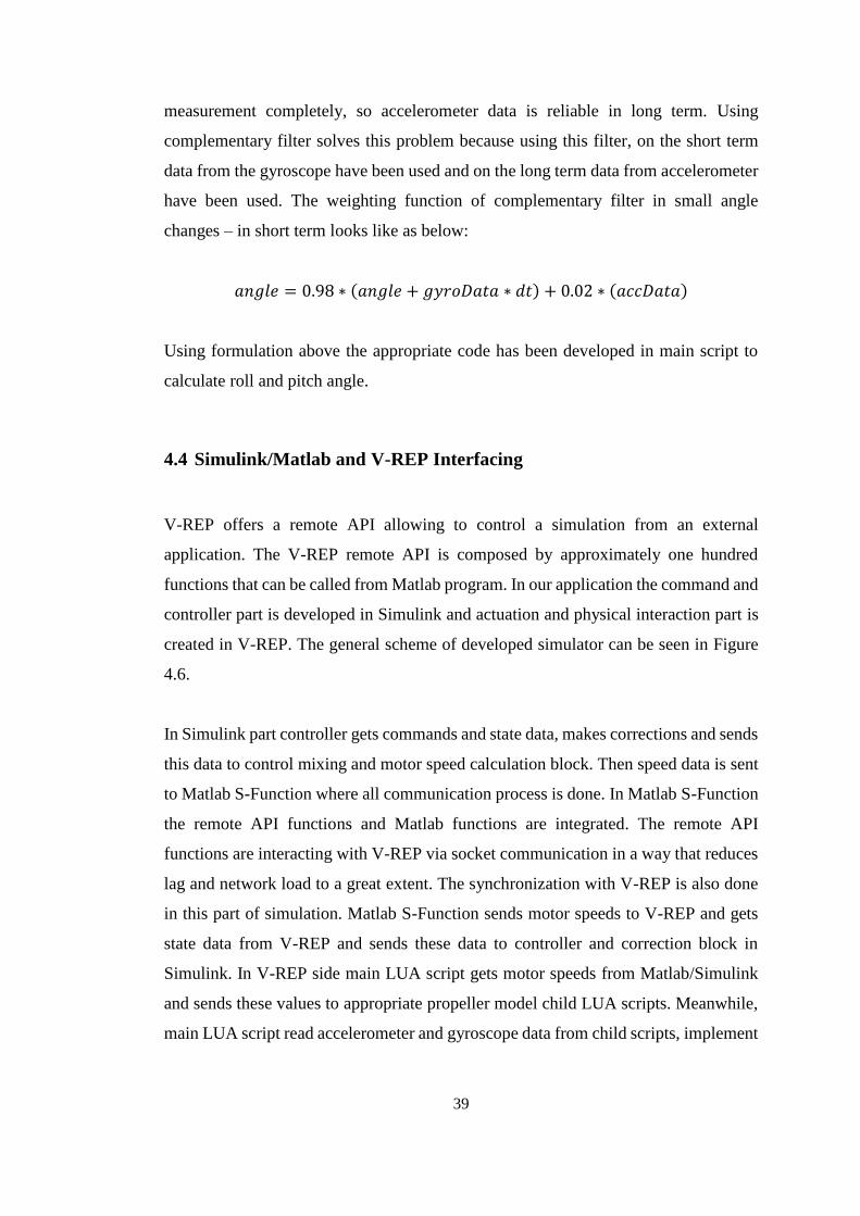
4.4 Simulink/Matlab and V-REP Interfacing

V-REP offers a remote API allowing to control a simulation from an external

application. The V-REP remote API is composed by approximately one hundred

functions that can be called from Matlab program. In our application the command and

controller part is developed in Simulink and actuation and physical interaction part is

created in V-REP. The general scheme of developed simulator can be seen in Figure

4.6.

In Simulink part controller gets commands and state data, makes corrections and sends

this data to control mixing and motor speed calculation block. Then speed data is sent

to Matlab S-Function where all communication process is done. In Matlab S-Function

the remote API functions and Matlab functions are integrated. The remote API

functions are interacting with V-REP via socket communication in a way that reduces

lag and network load to a great extent. The synchronization with V-REP is also done

in this part of simulation. Matlab S-Function sends motor speeds to V-REP and gets

state data from V-REP and sends these data to controller and correction block in

Simulink. In V-REP side main LUA script gets motor speeds from Matlab/Simulink

and sends these values to appropriate propeller model child LUA scripts. Meanwhile,

main LUA script read accelerometer and gyroscope data from child scripts, implement

40

complementary filter to these data and calculate roll and pitch angles. On the other

hand, it also gets absolute positions (x,y,z) and absolute velocities (u,v,w) of quadrotor,

combining them with angle (φ,θ,ψ) and angular velocity (p,q,r) data and sends them

to Simulink/Matlab application. The visualization of processed data is done both in

Simulink/Matlab and V-REP application.

Figure 4.6.General simulator operation diagram

41

CHAPTER 5

5. SIMULATION RESULTS

5.1 Simulation Results of Simulink/Matlab and V-REP Integration

Afterwards interfacing the Simulink/Matlab with V-REP controller tuning and flight

simulations trials have done. Processing with hand tuning and referring to Karwoski’s

studies [13] PID gains have been determined and can be seen in Table 5.1.

Table 5.1.Tuned PID gains

Gains Hover Roll Angle Pitch

Kp 16 25 25

Ki 1 0 0

Kd 10 6 6

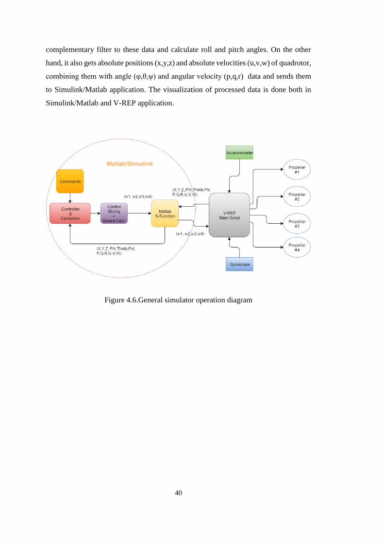
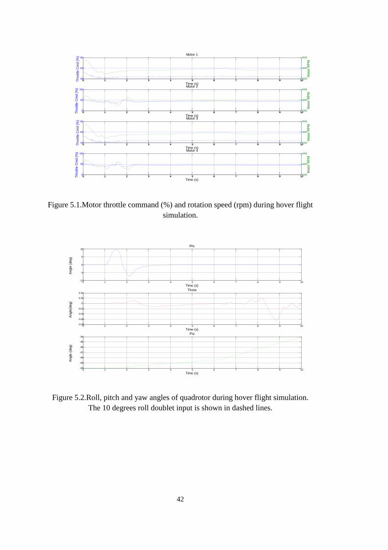
After tuning PID gains some flight conditions have been tested in simulator. One of

them is to hover from 1 m to 1.5 m and 10 degree roll angle doublet input in 1 sec. The

input command and motor command and state results can be seen in figures below.

42


simulation.

Figure 5.2.Roll, pitch and yaw angles of quadrotor during hover flight simulation.

The 10 degrees roll doublet input is shown in dashed lines.

0 1 2 3 4 5 6 7 8 9 1040

60

80

Time (s)

Thro

ttle

Cm

d (

%) Motor 1

0 1 2 3 4 5 6 7 8 9 103500

4000

4500

Moto

r R

PM

0 1 2 3 4 5 6 7 8 9 100

50

100

Time (s)

Thro

ttle

Cm

d (

%) Motor 2

0 1 2 3 4 5 6 7 8 9 103000

4000

5000

Moto

r R

PM

0 1 2 3 4 5 6 7 8 9 1040

60

80

Time (s)

Thro

ttle

Cm

d (

%) Motor 3

0 1 2 3 4 5 6 7 8 9 103500

4000

4500

Moto

r R

PM

0 1 2 3 4 5 6 7 8 9 100

50

100

Time (s)

Thro

ttle

Cm

d (

%) Motor 4

0 1 2 3 4 5 6 7 8 9 103000

4000

5000

Moto

r R

PM

0 1 2 3 4 5 6 7 8 9 10-10

-5

0

5

10

Time (s)

Angle

(deg)

Phi

0 1 2 3 4 5 6 7 8 9 10-0.08

-0.06

-0.04

-0.02

0

0.02

0.04

Time (s)

Angle

(deg)

Theta

0 1 2 3 4 5 6 7 8 9 10-90

-89

-88

-87

-86

-85

-84

Time (s)

Angle

(deg)

Psi

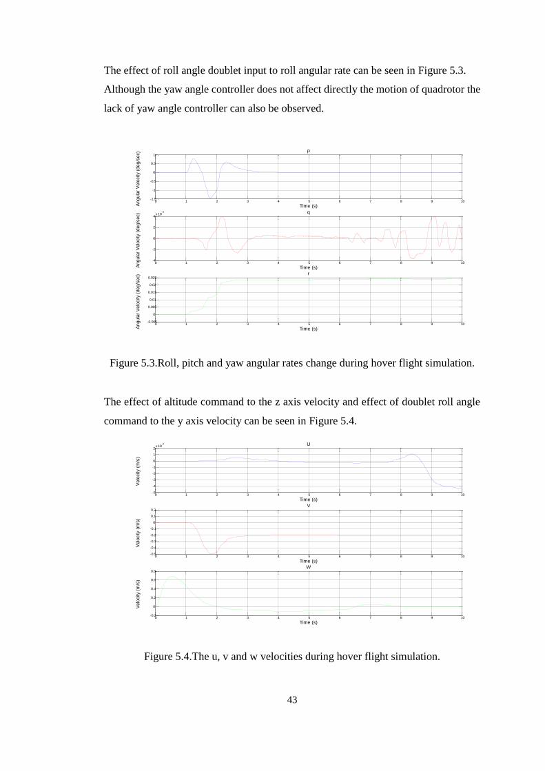
43

The effect of roll angle doublet input to roll angular rate can be seen in Figure 5.3.

Although the yaw angle controller does not affect directly the motion of quadrotor the

lack of yaw angle controller can also be observed.

Figure 5.3.Roll, pitch and yaw angular rates change during hover flight simulation.

The effect of altitude command to the z axis velocity and effect of doublet roll angle

command to the y axis velocity can be seen in Figure 5.4.

Figure 5.4.The u, v and w velocities during hover flight simulation.

0 1 2 3 4 5 6 7 8 9 10-1.5

-1

-0.5

0

0.5

1

Time (s)Angula

r V

elo

city (

deg/s

ec) p

0 1 2 3 4 5 6 7 8 9 10-4

-2

0

2

4x 10

-3

Time (s)Angula

r V

elo

city (

deg/s

ec) q

0 1 2 3 4 5 6 7 8 9 10-0.005

0

0.005

0.01

0.015

0.02

0.025

Time (s)Angula

r V

elo

city (

deg/s

ec) r

0 1 2 3 4 5 6 7 8 9 10-5

-4

-3

-2

-1

0

1

2x 10

-3

Time (s)

Velo

city (

m/s

)

U

0 1 2 3 4 5 6 7 8 9 10-0.5

-0.4

-0.3

-0.2

-0.1

0

0.1

0.2

Time (s)

Velo

city (

m/s

)

V

0 1 2 3 4 5 6 7 8 9 10-0.2

0

0.2

0.4

0.6

0.8

Time (s)

Velo

city (

m/s

)

W

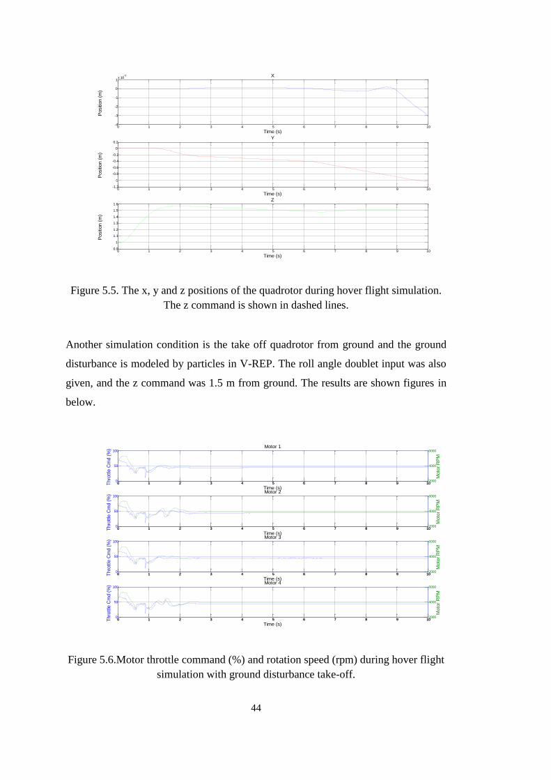
44

Figure 5.5. The x, y and z positions of the quadrotor during hover flight simulation.

The z command is shown in dashed lines.

Another simulation condition is the take off quadrotor from ground and the ground

disturbance is modeled by particles in V-REP. The roll angle doublet input was also

given, and the z command was 1.5 m from ground. The results are shown figures in

below.


simulation with ground disturbance take-off.

0 1 2 3 4 5 6 7 8 9 10-4

-3

-2

-1

0

1x 10

-3

Time (s)

Positio

n (

m)

X

0 1 2 3 4 5 6 7 8 9 10-1.2

-1

-0.8

-0.6

-0.4

-0.2

0

0.2

Time (s)

Positio

n (

m)

Y

0 1 2 3 4 5 6 7 8 9 100.9

1

1.1

1.2

1.3

1.4

1.5

1.6

Time (s)

Positio

n (

m)

Z

0 1 2 3 4 5 6 7 8 9 100

50

100

Time (s)

Thro

ttle

Cm

d (

%) Motor 1

0 1 2 3 4 5 6 7 8 9 102000

4000

6000

Moto

r R

PM

0 1 2 3 4 5 6 7 8 9 100

50

100

Time (s)

Thro

ttle

Cm

d (

%) Motor 2

0 1 2 3 4 5 6 7 8 9 102000

4000

6000

Moto

r R

PM

0 1 2 3 4 5 6 7 8 9 100

50

100

Time (s)

Thro

ttle

Cm

d (

%) Motor 3

0 1 2 3 4 5 6 7 8 9 102000

4000

6000

Moto

r R

PM

0 1 2 3 4 5 6 7 8 9 100

50

100

Time (s)

Thro

ttle

Cm

d (

%) Motor 4

0 1 2 3 4 5 6 7 8 9 102000

4000

6000

Moto

r R

PM

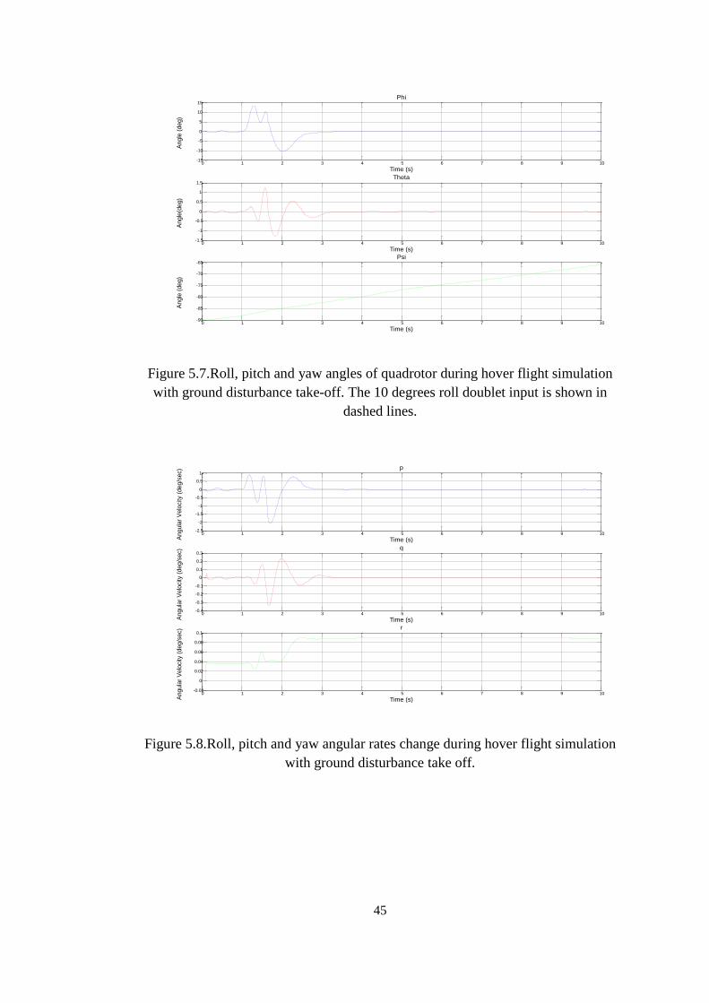
45

Figure 5.7.Roll, pitch and yaw angles of quadrotor during hover flight simulation

with ground disturbance take-off. The 10 degrees roll doublet input is shown in

dashed lines.

Figure 5.8.Roll, pitch and yaw angular rates change during hover flight simulation

with ground disturbance take off.

0 1 2 3 4 5 6 7 8 9 10-15

-10

-5

0

5

10

15

Time (s)

Angle

(deg)

Phi

0 1 2 3 4 5 6 7 8 9 10-1.5

-1

-0.5

0

0.5

1

1.5

Time (s)

Angle

(deg)

Theta

0 1 2 3 4 5 6 7 8 9 10-90

-85

-80

-75

-70

-65

Time (s)

Angle

(deg)

Psi

0 1 2 3 4 5 6 7 8 9 10-2.5

-2

-1.5

-1

-0.5

0

0.5

1

Time (s)Angula

r V

elo

city (

deg/s

ec) p

0 1 2 3 4 5 6 7 8 9 10-0.4

-0.3

-0.2

-0.1

0

0.1

0.2

0.3

Time (s)Angula

r V

elo

city (

deg/s

ec) q

0 1 2 3 4 5 6 7 8 9 10-0.02

0

0.02

0.04

0.06

0.08

0.1

Time (s)Angula

r V

elo

city (

deg/s

ec) r

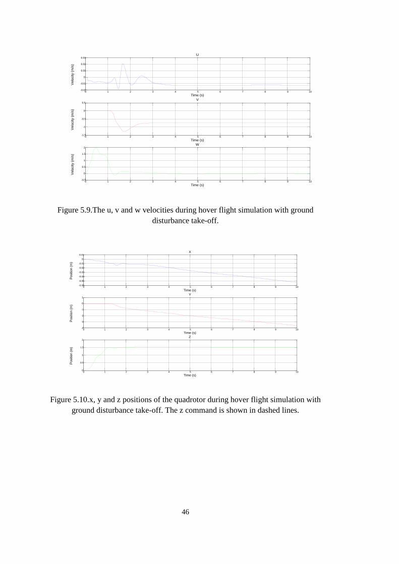
46

Figure 5.9.The u, v and w velocities during hover flight simulation with ground

disturbance take-off.

Figure 5.10.x, y and z positions of the quadrotor during hover flight simulation with

ground disturbance take-off. The z command is shown in dashed lines.

0 1 2 3 4 5 6 7 8 9 10-0.02

-0.01

0

0.01

0.02

0.03

Time (s)

Velo

city (

m/s

)

U

0 1 2 3 4 5 6 7 8 9 10-1.5

-1

-0.5

0

0.5

Time (s)

Velo

city (

m/s

)

V

0 1 2 3 4 5 6 7 8 9 10-0.5

0

0.5

1

1.5

2

Time (s)

Velo

city (

m/s

)

W

0 1 2 3 4 5 6 7 8 9 10-0.06

-0.05

-0.04

-0.03

-0.02

-0.01

0

0.01

Time (s)

Positio

n (

m)

X

0 1 2 3 4 5 6 7 8 9 10-4

-3

-2

-1

0

1

Time (s)

Positio

n (

m)

Y

0 1 2 3 4 5 6 7 8 9 100

0.5

1

1.5

2

Time (s)

Positio

n (

m)

Z

47

5.2 Experimental Setup for Quadrotor Flight Test

After simulation results there is need to validate the dynamic, sensor data and control

algorithm of a quadrotor. For this purpose basic experimental setup was built. The

similar experimental setup was built in [29] for test of vertical take-off and landing

(VTOL) air vehicle. In this part explanation of this experimental setup is given with

illustrations. The quadrotor that is used in these experiments is AscTec Hummingbird.

The quadrotor test were made in indoor conditions. So there were need to take safety

cautions and limit the range of motion of a quadrotor. Experimental test setup was built

with limited motion range.

Figure 5.11. The assembly view of experimental setup allowing movement in

translation axes.

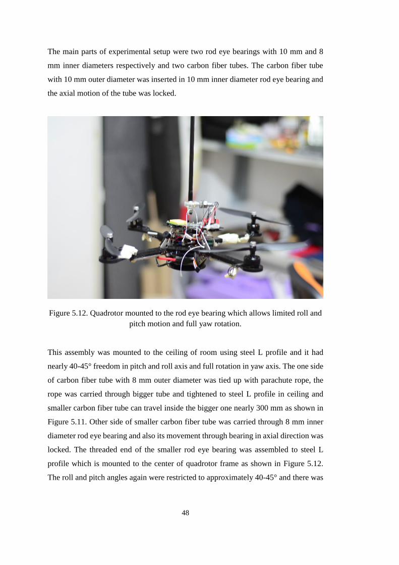
48

The main parts of experimental setup were two rod eye bearings with 10 mm and 8

mm inner diameters respectively and two carbon fiber tubes. The carbon fiber tube

with 10 mm outer diameter was inserted in 10 mm inner diameter rod eye bearing and

the axial motion of the tube was locked.

Figure 5.12. Quadrotor mounted to the rod eye bearing which allows limited roll and

pitch motion and full yaw rotation.

This assembly was mounted to the ceiling of room using steel L profile and it had

nearly 40-45° freedom in pitch and roll axis and full rotation in yaw axis. The one side

of carbon fiber tube with 8 mm outer diameter was tied up with parachute rope, the

rope was carried through bigger tube and tightened to steel L profile in ceiling and

smaller carbon fiber tube can travel inside the bigger one nearly 300 mm as shown in

Figure 5.11. Other side of smaller carbon fiber tube was carried through 8 mm inner

diameter rod eye bearing and also its movement through bearing in axial direction was

locked. The threaded end of the smaller rod eye bearing was assembled to steel L

profile which is mounted to the center of quadrotor frame as shown in Figure 5.12.

The roll and pitch angles again were restricted to approximately 40-45° and there was

49

full rotation in yaw axis. The height that quadrotor can travel from its hanger position

was approximately 300 mm. The quadrotor can also move in limited range in lateral

and longitudinal directions due to bigger rod eye bearing. In Figure 5.13 the visual is

shown from flight tests.

Figure 5.13. The view of motion of quadrotor in flight tests

There also fixed type experimental setup was built. In this setup the lateral,

longitudinal and altitude motions of quadrotor was locked. There were only roll and

pitch motions which were limited to approximately 40-45° and full range yaw motion

was allowed. The setup comprise the stiff wood which was mounted to the ceiling of

room using steel L profile. The carbon fiber with 8 mm outer diameter was fixed to

the wood with steel bracelets and ensured that no movement and rotation in any

direction (Figure 5.14). The rod eye bearing with 8 mm inner diameter was mounted

to the end of carbon tube and movement along the altitude direction was locked. The

threaded end of the smaller rod eye bearing again was assembled to steel L profile

which was mounted to the center of quadrotor frame as shown in Figure 5.15.

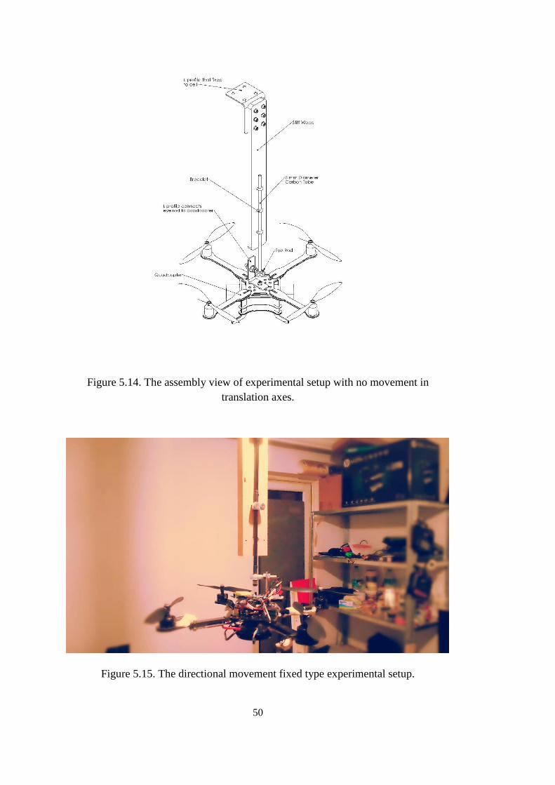
50

Figure 5.14. The assembly view of experimental setup with no movement in

translation axes.

Figure 5.15. The directional movement fixed type experimental setup.

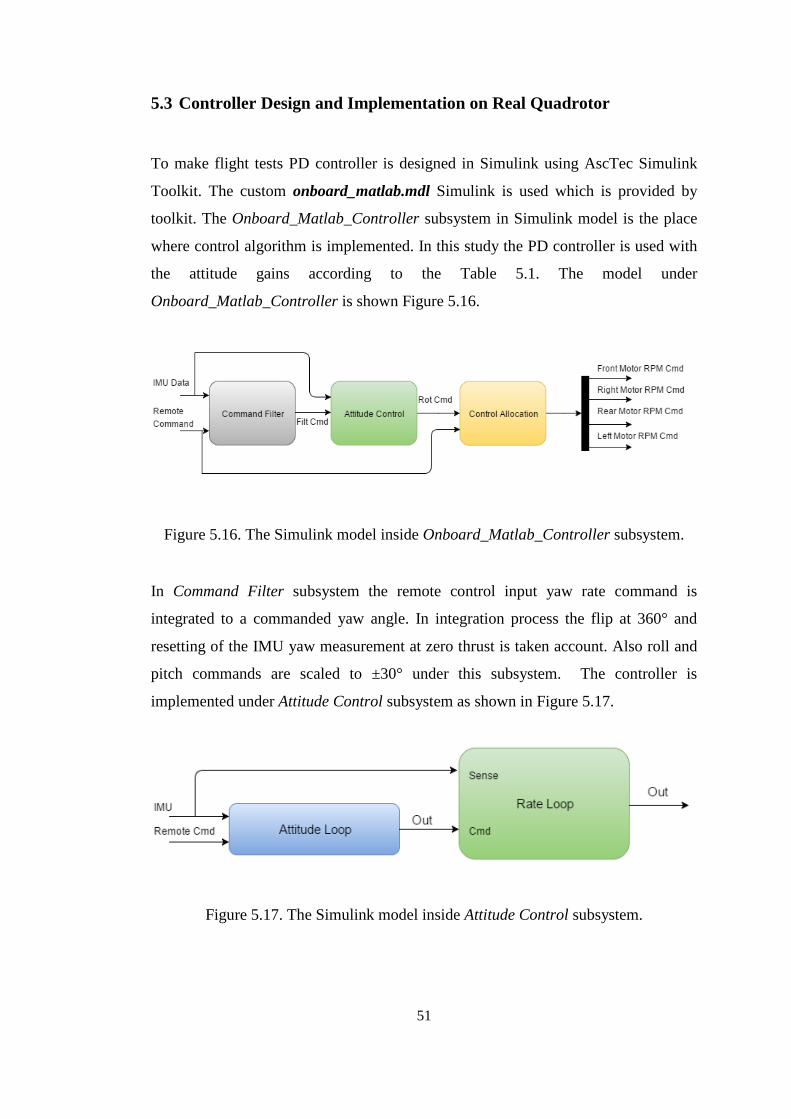
51

5.3 Controller Design and Implementation on Real Quadrotor

To make flight tests PD controller is designed in Simulink using AscTec Simulink

Toolkit. The custom onboard_matlab.mdl Simulink is used which is provided by

toolkit. The Onboard_Matlab_Controller subsystem in Simulink model is the place

where control algorithm is implemented. In this study the PD controller is used with

the attitude gains according to the Table 5.1. The model under

Onboard_Matlab_Controller is shown Figure 5.16.

Figure 5.16. The Simulink model inside Onboard_Matlab_Controller subsystem.

In Command Filter subsystem the remote control input yaw rate command is

integrated to a commanded yaw angle. In integration process the flip at 360° and

resetting of the IMU yaw measurement at zero thrust is taken account. Also roll and

pitch commands are scaled to ±30° under this subsystem. The controller is

implemented under Attitude Control subsystem as shown in Figure 5.17.

Figure 5.17. The Simulink model inside Attitude Control subsystem.

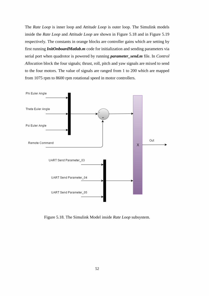
52

The Rate Loop is inner loop and Attitude Loop is outer loop. The Simulink models

inside the Rate Loop and Attitude Loop are shown in Figure 5.18 and in Figure 5.19

respectively. The constants in orange blocks are controller gains which are setting by

first running InitOnboardMatlab.m code for initialization and sending parameters via

serial port when quadrotor is powered by running parameter_send.m file. In Control

Allocation block the four signals; thrust, roll, pitch and yaw signals are mixed to send

to the four motors. The value of signals are ranged from 1 to 200 which are mapped

from 1075 rpm to 8600 rpm rotational speed in motor controllers.

Figure 5.18. The Simulink Model inside Rate Loop subsystem.

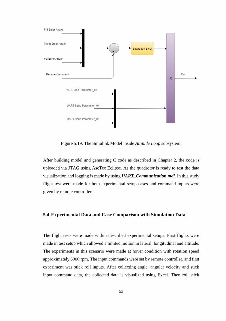
53

Figure 5.19. The Simulink Model inside Attitude Loop subsystem.

After building model and generating C code as described in Chapter 2, the code is

uploaded via JTAG using AscTec Eclipse. As the quadrotor is ready to test the data

visualization and logging is made by using UART_Communication.mdl. In this study

flight test were made for both experimental setup cases and command inputs were

given by remote controller.

5.4 Experimental Data and Case Comparison with Simulation Data

The flight tests were made within described experimental setups. First flights were

made in test setup which allowed a limited motion in lateral, longitudinal and altitude.

The experiments in this scenario were made at hover condition with rotation speed

approximately 3900 rpm. The input commands were set by remote controller, and first

experiment was stick roll inputs. After collecting angle, angular velocity and stick

input command data, the collected data is visualized using Excel. Then roll stick

54

command is imported to Simulink model using Signal Builder tool. The Simulink

model is interfaced with quadrotor model that created in V-REP, then simulation had

ran and data were collected. The roll stick input and according real quadrotor measured

roll angle and V-REP quadrotor model logged angle are shown in Figure 5.20.

Figure 5.20. The roll angle (deg) response to roll stick input in directional motion

free test setup.

From the graph it is seen that there is delay between measured and simulated roll angle.

The one of the main reasons of that is the difference between real quadrotor IMU and

the IMU that picked up from sensor models of V-REP. Also in V-REP scene the

quadrotor is in free mode and not hanged to any tube. The moment of inertia of rod

eye bearings, carbon tubes and small L profile can cause this type small changes in

response dynamics. The response of roll angular velocity to this roll stick input in real

quadrotor and V-REP quadrotor model is visualized in Figure 5.21. Again the delay

and oscillation difference in the measurement of real and simulated roll angular

velocity shows the minor differences between IMU models.

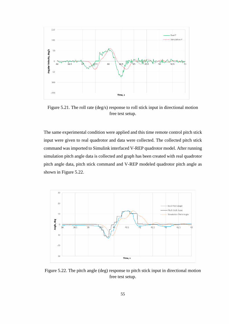
55

Figure 5.21. The roll rate (deg/s) response to roll stick input in directional motion

free test setup.

The same experimental condition were applied and this time remote control pitch stick

input were given to real quadrotor and data were collected. The collected pitch stick

command was imported to Simulink interfaced V-REP quadrotor model. After running

simulation pitch angle data is collected and graph has been created with real quadrotor

pitch angle data, pitch stick command and V-REP modeled quadrotor pitch angle as



free test setup.

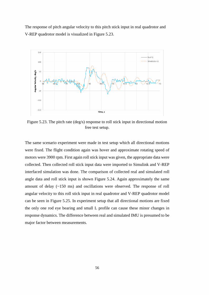
56

The response of pitch angular velocity to this pitch stick input in real quadrotor and

V-REP quadrotor model is visualized in Figure 5.23.


free test setup.

The same scenario experiment were made in test setup which all directional motions

were fixed. The flight condition again was hover and approximate rotating speed of

motors were 3900 rpm. First again roll stick input was given, the appropriate data were

collected. Then collected roll stick input data were imported to Simulink and V-REP

interfaced simulation was done. The comparison of collected real and simulated roll

angle data and roll stick input is shown Figure 5.24. Again approximately the same

amount of delay (~150 ms) and oscillations were observed. The response of roll

angular velocity to this roll stick input in real quadrotor and V-REP quadrotor model

can be seen in Figure 5.25. In experiment setup that all directional motions are fixed

the only one rod eye bearing and small L profile can cause these minor changes in

response dynamics. The difference between real and simulated IMU is presumed to be

major factor between measurements.

57

Figure 5.24. The roll angle (deg) response to roll stick input in directional motion

fixed test setup.

Figure 5.25. The roll rate (deg/s) response to roll stick input in directional motion

fixed test setup.

The same experiment conditions in directional motion fixed experiment setup were

applied and this time pitch stick input was given. From collected data pitch stick input

signal was imported to Simulink model which is interfaced with V-REP built quadrotor

model. The response of real and simulated pitch angels and angular rates can be seen

in Figure 5.26 and in Figure 5.27 respectively.

58


fixed test setup.


fixed test setup.

59

5.5 Collision Avoidance and Wall Following

After the verification of the quadrotor in V-REP environment the study has been done

regarding to use the sensor capability of V-REP. According to this study the collision

avoidance subject has been selected and final object is simple wall following controller

design. The ultrasonic sensor has been chosen for object detection due to its application

simplicity and the possibility of fast real life implementation in near future. As a sensor

Maxbotix XL-MaxSonar-AE0 MB1300 has been selected [30] and the sensor is

modeled in V-REP using proximity sensor specifications.

Figure 5.28. Maxbotix XL-MaxSonar-AE0 MB1300 [30].

Four ultrasonic sensors have been inserted on quadrotor model in V-REP in

perpendicular manner in four directions for sensing the obstacles or wall in 2D. The

fifth ultrasonic sensor has been inserted for measurement of altitude from the ground.

The orientation of the sensors on quadrotor model is shown in Figure 5.29. Afterwards

adding wall model into V-REP simulation environment has been completed. On the

controller side in outside loop the velocity has been controlled in x and y directions.

According to the commands coming from outside control loop in inner loop the roll,

pitch, yaw and altitude have been controlled. In design stages of controller, obstacle

avoidance and wall following algorithms, step by step implementations and trials have

been done in Simulink/Matlab interfaced V-REP environment. This type of

implementation shows the usefulness of 3D physically modeled environment (V-REP)

and easy design and implementation of controller platform (Simulink/Matlab).

60

Figure 5.29. Ultrasonic sensor orientation on quadrotor in V-REP

The velocity data in x and y directions has been gathered from four ultrasonic sensors

in V-REP LUA script. The velocity in one direction has been calculated by dividing

ultrasonic distance measurement difference between current and previous loop to

simulation time step. The range of ultrasonic sensor used in this study is 7.65 m and it

has 1 cm resolution. In velocity calculation algorithm quadrotor assumes middle of the

room as origin, if the quadrotor is in positive x direction side it uses the measurement

of ultrasonic sensor that is mounted in that direction and if it is in negative x direction

side it uses the measurement of ultrasonic sensor that is mounted in that direction. The

same procedure has been applied to y direction also. The velocity calculation algorithm

considers the roll, pitch and yaw angles corrections while evaluating the measured

distances.

In the first step of the development process aim was to make velocity control and stop

after referenced wall distance. The initial command was pitch angle that to travel in

positive x direction. The pitch angle command was the function of the distance to the

wall and decreased as it got closer to the wall. After referenced distance to the wall

was reached, the quadrotor slowed down and stopped with referenced constant

distance (3 m) to the wall. The velocity control was done using PD controller. The

61

change of roll, pitch, and yaw angles due to velocity command and response of the

motors can be seen in figures below.

Figure 5.30. Roll, pitch and yaw angles of quadrotor during free flight and obstacle

detection.

Figure 5.31. Motor throttle command (%) and rotation speed (rpm) during free flight

and obstacle detection.

0 1 2 3 4 5 6 7 8 9-0.1

-0.05

0

0.05

0.1

Time (s)

Angle

(deg)

Phi

0 1 2 3 4 5 6 7 8 9-6

-4

-2

0

2

4

6

Time (s)

Angle

(deg)

Theta

0 1 2 3 4 5 6 7 8 9-90.6

-90.4

-90.2

-90

-89.8

Time (s)

Angle

(deg)

Psi

0 1 2 3 4 5 6 7 8 90

50

100

Time (s)

Thro

ttle

Cm

d (

%) Motor 1

0 1 2 3 4 5 6 7 8 93500

4000

4500

Moto

r R

PM

0 1 2 3 4 5 6 7 8 90

50

100

Time (s)

Thro

ttle

Cm

d (

%) Motor 2

0 1 2 3 4 5 6 7 8 93500

4000

4500

Moto

r R

PM

0 1 2 3 4 5 6 7 8 90

50

100

Time (s)

Thro

ttle

Cm

d (

%) Motor 3

0 1 2 3 4 5 6 7 8 93500

4000

4500

Moto

r R

PM

0 1 2 3 4 5 6 7 8 90

50

100

Time (s)

Thro

ttle

Cm

d (

%) Motor 4

0 1 2 3 4 5 6 7 8 93500

4000

4500

Moto

r R

PM

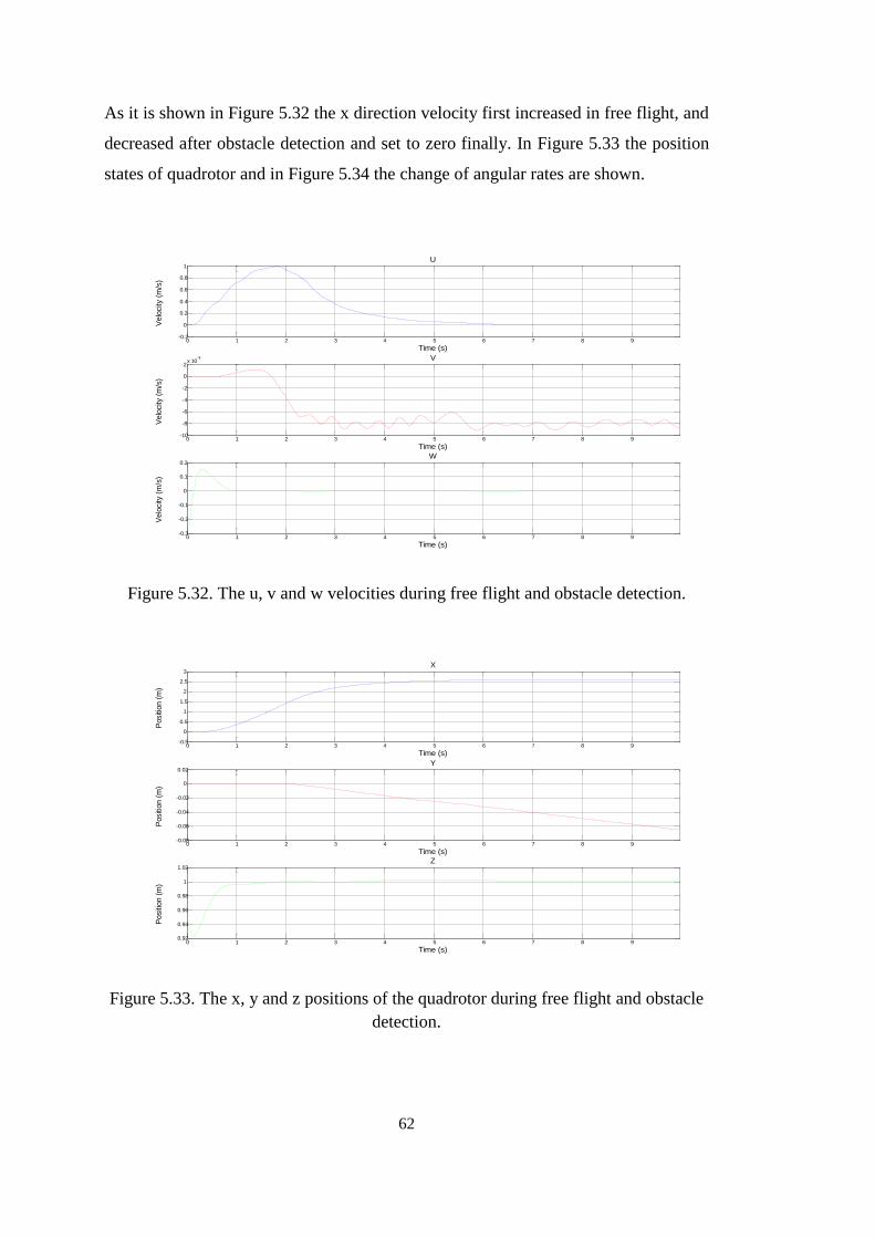
62

As it is shown in Figure 5.32 the x direction velocity first increased in free flight, and

decreased after obstacle detection and set to zero finally. In Figure 5.33 the position

states of quadrotor and in Figure 5.34 the change of angular rates are shown.

Figure 5.32. The u, v and w velocities during free flight and obstacle detection.

Figure 5.33. The x, y and z positions of the quadrotor during free flight and obstacle

detection.

0 1 2 3 4 5 6 7 8 9-0.2

0

0.2

0.4

0.6

0.8

1

Time (s)

Velo

city (

m/s

)

U

0 1 2 3 4 5 6 7 8 9-10

-8

-6

-4

-2

0

2x 10

-3

Time (s)

Velo

city (

m/s

)

V

0 1 2 3 4 5 6 7 8 9-0.3

-0.2

-0.1

0

0.1

0.2

Time (s)

Velo

city (

m/s

)

W

0 1 2 3 4 5 6 7 8 9-0.5

0

0.5

1

1.5

2

2.5

3

Time (s)

Positio

n (

m)

X

0 1 2 3 4 5 6 7 8 9-0.08

-0.06

-0.04

-0.02

0

0.02

Time (s)

Positio

n (

m)

Y

0 1 2 3 4 5 6 7 8 90.92

0.94

0.96

0.98

1

1.02

Time (s)

Positio

n (

m)

Z

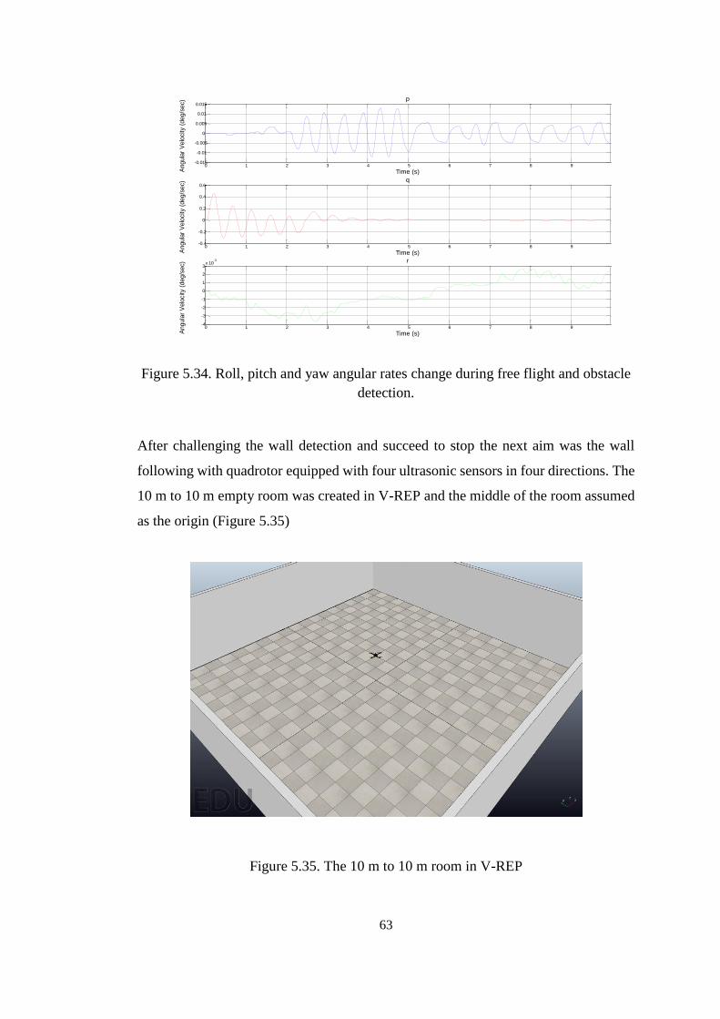
63

Figure 5.34. Roll, pitch and yaw angular rates change during free flight and obstacle

detection.

After challenging the wall detection and succeed to stop the next aim was the wall

following with quadrotor equipped with four ultrasonic sensors in four directions. The

10 m to 10 m empty room was created in V-REP and the middle of the room assumed

as the origin (Figure 5.35)

Figure 5.35. The 10 m to 10 m room in V-REP

0 1 2 3 4 5 6 7 8 9-0.015

-0.01

-0.005

0

0.005

0.01

0.015

Time (s)Angula

r V

elo

city (

deg/s

ec) p

0 1 2 3 4 5 6 7 8 9-0.4

-0.2

0

0.2

0.4

0.6

Time (s)Angula

r V

elo

city (

deg/s

ec) q

0 1 2 3 4 5 6 7 8 9-4

-3

-2

-1

0

1

2

3x 10

-3

Time (s)Angula

r V

elo

city (

deg/s

ec) r

64

Using four sensor data the logic algorithm was developed with five states. The

algorithm developed in Simulink gets roll, pitch and yaw angles, ultrasonic sensors

data and velocities from V-REP. The general scheme of algorithm is shown in Figure

5.36.

Figure 5.36. The general scheme of wall following mode with varying travel speed

In State 1 the quadrotor is in the middle area of the room and it is in free flight mode.

In free flight mode the quadrotor travel in positive x direction with pitch angle

command and sets its y direction velocity to zero by PD controller. The pitch angle

command is the function of the distance to the wall that measured by the ultrasonic

sensor mounted on move direction and decreases as it got closer to the wall (Figure

5.37). After the referenced 3 m wall distance is reached algorithm switches to State 2.

In State 2 this time the quadrotor starts to move in negative y direction and sets its x

direction velocity to zero by PD controller. The roll angle command like in State 1 is

the function of the distance to the wall that measured by the ultrasonic sensor mounted

on move direction and decreases as it got closer to the wall (Figure 5.38). The

algorithm continues with the same logic by following State 3, State 4 and State 5. The

controllers inside the State 3 and State 4 are like State 1 and State 2 respectively with

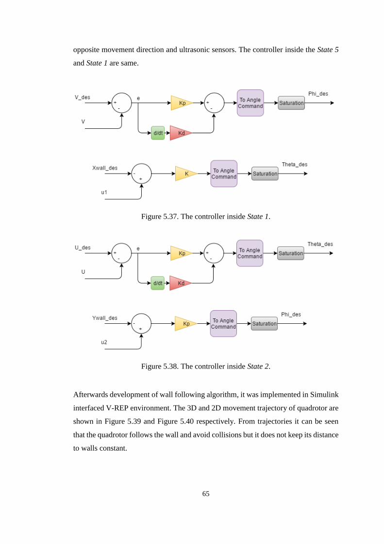
65

opposite movement direction and ultrasonic sensors. The controller inside the State 5

and State 1 are same.

Figure 5.37. The controller inside State 1.

Figure 5.38. The controller inside State 2.

Afterwards development of wall following algorithm, it was implemented in Simulink

interfaced V-REP environment. The 3D and 2D movement trajectory of quadrotor are

shown in Figure 5.39 and Figure 5.40 respectively. From trajectories it can be seen

that the quadrotor follows the wall and avoid collisions but it does not keep its distance

to walls constant.

66


varying travel speed.


varying travel speed.

The change of roll, pitch and yaw angles and angular rates according to the trajectory

shown above are shown in Figure 5.41 and Figure 5.42 respectively.

-5-4

-3-2

-10

12

34

5

-5

-4

-3

-2

-1

0

1

2

3

4

5

0

0.2

0.4

0.6

0.8

1

1.2

1.4

1.6

1.8

2

X Position (m)

X,Y and Z Positions of Quadrotor in 10x10 Room

Y Position (m)

Z P

ositio

n (

m)

-5 -4 -3 -2 -1 0 1 2 3 4 5-5

-4

-3

-2

-1

0

1

2

3

4

5

X Position (m)

Y P

ositio

n (

m)

X and Y Positions of Quadrotor in 10x10 Room

67

Figure 5.41. Roll, pitch and yaw angles of wall following quadrotor in 10 m to 10 m

room with varying travel speed.

Figure 5.42. Roll, pitch and yaw angular rates change of wall following quadrotor in

10 m to 10 m room with varying travel speed.

The variation of velocities in x and y directions can be observed from Figure 5.43. The

positions of quadrotor response to these velocity variations are shown in Figure 5.44.

0 10 20 30 40 50 60-5

0

5

Time (s)

Angle

(deg)

Phi

0 10 20 30 40 50 60-5

0

5

Time (s)

Angle

(deg)

Theta

0 10 20 30 40 50 60-91

-90

-89

-88

-87

-86

-85

-84

Time (s)

Angle

(deg)

Psi

0 10 20 30 40 50 60-0.4

-0.2

0

0.2

0.4

Time (s)Angula

r V

elo

city (

deg/s

ec) p

0 10 20 30 40 50 60-0.4

-0.2

0

0.2

0.4

Time (s)Angula

r V

elo

city (

deg/s

ec) q

0 10 20 30 40 50 60-0.01

-0.005

0

0.005

0.01

0.015

Time (s)Angula

r V

elo

city (

deg/s

ec) r

68

Figure 5.43. The u, v and w velocities of wall following quadrotor in 10 m to 10 m


Figure 5.44. The x, y and z positions of wall following quadrotor in 10 m to 10 m


The response of the motors according this varying velocity travel mode is shown in

Figure 5.45.

0 10 20 30 40 50 60-1.5

-1

-0.5

0

0.5

1

1.5

2

Time (s)

Velo

city (

m/s

)

U

0 10 20 30 40 50 60-1.5

-1

-0.5

0

0.5

1

1.5

Time (s)

Velo

city (

m/s

)

V

0 10 20 30 40 50 60-0.2

-0.15

-0.1

-0.05

0

0.05

0.1

0.15

Time (s)

Velo

city (

m/s

)

W

0 10 20 30 40 50 60-4

-2

0

2

4

Time (s)

Positio

n (

m)

X

0 10 20 30 40 50 60-4

-2

0

2

4

Time (s)

Positio

n (

m)

Y

0 10 20 30 40 50 600.92

0.94

0.96

0.98

1

1.02

Time (s)

Positio

n (

m)

Z

69


quadrotor in 10 m to 10 m room with varying travel speed.

The final development objective was again following the wall with approximately 3 m

constant distance to the wall. The control logic is similar with previous one but this

time velocity commands are constant, and in state switches the set value of velocity

commands change. The general scheme of the developed algorithm is shown in Figure

5.46. The If..Else Conditioning block switch states according to the distance to the wall

and outputs of block are velocity commands in x and y directions. The Velocity

Controller block contains two PD controller for u and v velocity commands. The

scheme of controllers is shown in Figure 5.47.

0 10 20 30 40 50 600

50

100

Time (s)

Thro

ttle

Cm

d (

%) Motor 1

0 10 20 30 40 50 603500

4000

4500

Moto

r R

PM

0 10 20 30 40 50 600

50

100

Time (s)

Thro

ttle

Cm

d (

%) Motor 2

0 10 20 30 40 50 603500

4000

4500

Moto

r R

PM

0 10 20 30 40 50 600

50

100

Time (s)

Thro

ttle

Cm

d (

%) Motor 3

0 10 20 30 40 50 603500

4000

4500

Moto

r R

PM

0 10 20 30 40 50 600

50

100

Time (s)

Thro

ttle

Cm

d (

%) Motor 4

0 10 20 30 40 50 603500

4000

4500

Moto

r R

PM

70

Figure 5.46. The general scheme of wall following mode with constant distance to

the wall.

Figure 5.47. The PD controller scheme inside Velocity Controller.

Afterwards implementation of developed algorithm to Simulink interfaced V-REP the

simulation results have been gathered. The 3D and 2D move trajectories of quadrotor

inside a 10 to 10 m room are shown in Figure 5.48 and Figure 5.49 respectively. It can

be observed that the quadrotor is approximately in constant distance to the wall.

71

Figure 5.48. 3D trajectory of wall following quadrotor holding constant distance to

the wall in 10 m to 10 m room.

Figure 5.49. 2D trajectory of wall following quadrotor holding constant distance to

the wall in 10 m to 10 m room.

The change of roll, pitch and yaw angles and angular rates according to the trajectory

shown above are shown in Figure 5.50 and Figure 5.51 respectively.

-5-4

-3-2

-10

12

34

5

-5

-4

-3

-2

-1

0

1

2

3

4

5

0

0.2

0.4

0.6

0.8

1

1.2

1.4

1.6

1.8

2

X Position (m)

X,Y and Z Positions of Quadrotor in 10x10 Room

Y Position (m)

Z P

ositio

n (

m)

-5 -4 -3 -2 -1 0 1 2 3 4 5-5

-4

-3

-2

-1

0

1

2

3

4

5

X Position (m)

Y P

ositio

n (

m)

X and Y Positions of Quadrotor in 10x10 Room

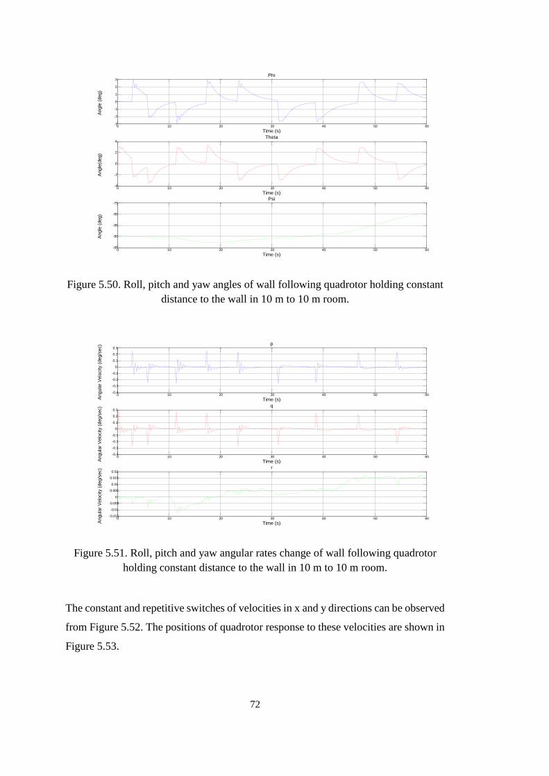
72

Figure 5.50. Roll, pitch and yaw angles of wall following quadrotor holding constant

distance to the wall in 10 m to 10 m room.

Figure 5.51. Roll, pitch and yaw angular rates change of wall following quadrotor

holding constant distance to the wall in 10 m to 10 m room.

The constant and repetitive switches of velocities in x and y directions can be observed

from Figure 5.52. The positions of quadrotor response to these velocities are shown in

Figure 5.53.

0 10 20 30 40 50 60-3

-2

-1

0

1

2

3

Time (s)

Angle

(deg)

Phi

0 10 20 30 40 50 60-4

-2

0

2

4

Time (s)

Angle

(deg)

Theta

0 10 20 30 40 50 60-95

-90

-85

-80

-75

Time (s)

Angle

(deg)

Psi

0 10 20 30 40 50 60-0.4

-0.3

-0.2

-0.1

0

0.1

0.2

0.3

Time (s)Angula

r V

elo

city (

deg/s

ec) p

0 10 20 30 40 50 60-0.4

-0.3

-0.2

-0.1

0

0.1

0.2

0.3

Time (s)Angula

r V

elo

city (

deg/s

ec) q

0 10 20 30 40 50 60-0.015

-0.01

-0.005

0

0.005

0.01

0.015

0.02

Time (s)Angula

r V

elo

city (

deg/s

ec) r

73

Figure 5.52. The u, v and w velocities of wall following quadrotor holding constant


Figure 5.53. The x, y and z positions of wall following quadrotor holding constant


The response of the motors according to this constant distance travel mode is shown

in Figure 5.54

0 10 20 30 40 50 60-1

-0.5

0

0.5

1

Time (s)

Velo

city (

m/s

)

U

0 10 20 30 40 50 60-1

-0.5

0

0.5

1

Time (s)

Velo

city (

m/s

)V

0 10 20 30 40 50 60-0.2

-0.15

-0.1

-0.05

0

0.05

0.1

0.15

Time (s)

Velo

city (

m/s

)

W

0 10 20 30 40 50 60-3

-2

-1

0

1

2

3

Time (s)

Positio

n (

m)

X

0 10 20 30 40 50 60-3

-2

-1

0

1

2

3

Time (s)

Positio

n (

m)

Y

0 10 20 30 40 50 600.94

0.95

0.96

0.97

0.98

0.99

1

1.01

Time (s)

Positio

n (

m)

Z

74


quadrotor holding constant distance to the wall in 10 m to 10 m room.

0 10 20 30 40 50 600

50

100

Time (s)

Thro

ttle

Cm

d (

%) Motor 1

0 10 20 30 40 50 603500

4000

4500

Moto

r R

PM

0 10 20 30 40 50 600

50

100

Time (s)

Thro

ttle

Cm

d (

%) Motor 2

0 10 20 30 40 50 603500

4000

4500

Moto

r R

PM

0 10 20 30 40 50 600

50

100

Time (s)

Thro

ttle

Cm

d (

%) Motor 3

0 10 20 30 40 50 603500

4000

4500

Moto

r R

PM

0 10 20 30 40 50 600

50

100

Time (s)

Thro

ttle

Cm

d (

%) Motor 4

0 10 20 30 40 50 603500

4000

4500

Moto

r R

PM

75

CHAPTER 6

6. CONCLUSION AND FUTURE WORK

In this thesis the easy use 3-D simulator is designed for the test of variety control

algorithms in AscTec Hummingbird quadrotor. First the dynamic model of the

quadrotor is derived and PID controller is designed in Simulink/Matlab platform.

Afterwards propeller model is created in V-REP relying on real test data and

experimental transfer function of motor propeller. The 3-D model of quadrotor is also

designed and accelerometer, gyroscope sensors, and GPS unit are added to quadrotor

model in V-REP. Then the controller in Simulink/Matlab is interfaced with quadrotor

model in V-REP and three dimensional physical environment interacted tests become

easier in this combined simulator. The first flight tests have been made in simulator.

In first case doublet input is given and the stabilization of vehicle in simulator is

satisfied in hover condition. Next step quadrotor is taken off from ground to

commanded height and again doublet input command is given and stabilization is

satisfied. In this simulation ground disturbance is modeled where random moved air

particles of V-REP included to propeller model. Then two case experimental setup has

been built for real quadrotor test flights. In first case experimental setup the directional

movements were settled free and input commands were given from remote controller,

and data were collected. Then stick commands were imported to Simulink interfaced

V-REP quadrotor model and regarding data were collected. In comparison of real and

simulated there approximately 150 ms delay was observed. One possible reason is the

difference between real and simulated IMU model. The next possible reason is

addition of some stuff on real quadrotor model due to experimental setup which can

effect dynamic response. It must be mentioned that simulations in V-REP was done in

free flight hover conditions. In second case experimental setup the directional motions

were fixed only rotational motions were allowed. The same test procedure was applied.

76

The results were similar and again approximately 150 ms delay was observed. As a

result the 3-D Simulink interfaced physical simulator for quadrotor is achieved and its

experimental validation has been done. The collision avoidance and wall following

studies were carried to show the capabilities of simulator infrastructure which is the

main object of this thesis. Ultrasonic distance sensors have been used for object or wall

detection. Step by step controller algorithm has been developed totally in safe and easy

manner. Using PD type velocity controller the wall following of quadrotor with

approximately constant distance to the wall is achieved.

For future author can recommend addition of more detailed IMU model. Other

classical and nonlinear control algorithms can be implemented in this simulator.

Adding 2-D, 3-D vision sensor can create chance for localization and mapping

algorithm tests. Advanced collision avoidance algorithms could also be developed in

this simulator infrastructure. After developing these algorithms the costly sensors can

be achieved and simulator based developed algorithms can be implemented on real

quadrotor.

77

REFERENCES

[1] G. Hoffmann, D. G. Rajnarayan, S. L. Waslander, D. Dostal, J. Jang and C. J.

Tomlin, "The Stanford testbed of autonomous rotorcraft for multi agent

control(STARMAC)," in Digital Avionics Systems Conference, 2004.

[2] G. M. Hoffman and H. Huang, "Quadrotor helicopter flight dynamics and control

theory and experiment.," American Institute of Aeronautics and Astronautics,

2007.

[3] P. Pounds, R. Mahony and P. Corke, "Modeling and Control of a Quad-Rotor

Robot," in Australian National University, Canberra, 2006.

[4] "Flying Machine Arena," Institute for Dynamic Systems and Control, ETH

Zurich, [Online]. Available: http:// http://flyingmachinearena.org/. [Accessed

May 2016].

[5] University of Pennsylvania, GRASP Lab., [Online]. Available:

http://www.gizmag.com/grasp-nano-quadrotor-robots-swarm/21302/.

[Accessed May 2016].

[6] M. J. Cutler, "Design and Control of an Autonomous Variable-Pitch Quadrotor

Helicopter," MIT M.Sc. thesis, Massachusetts, 2012.

[7] "Phantom 4," [Online]. Available: http://www.dji.com/product/phantom-

4/info#specs. [Accessed May 2016].

[8] [Online]. Available: http://www.draganfly.com/uav-helicopter/draganflyer-

x4p/specifications/. [Accessed May 2016].

[9] [Online]. Available: https://www.microdrones.com/en/products/md4-200/.


[10] [Online]. Available: http://ardrone2.parrot.com/. [Accessed May 2016].

[11] V. M. Martinez, "Modelling of the Flight Dynamics of a Quadrotor Helicopter,"

Cranfield University,M.Sc. thesis, Cranfield, 2007.

[12] M. Oliveira, "Modeling, Identification and Control of a Quadrotor Aircraft,"

Czech Technical University in Prague, M.Sc. thesis, Prague, 2011.

78

[13] K. Karwoski, "Quadrocopter Control Design and Flight Operation," NASA

USRP – Internship Final Report.

[14] G. Bardaro, A. Cucci, L. Bascetta and M. Matteucci, "A simulation based

architecture for the development of an autonomous all terrain vehicle," in 4th

International Conference, Bergamo, 2014.

[15] "PyQuadSim: An open-source Python Quadcopter Simulator for Linux,

Windows, and Mac OS X," [Online]. Available:

http://home.wlu.edu/~levys/software/pyquadsim/. [Accessed May 2016].

[16] "PyQuadSim Autopilot Scheme," [Online]. Available:

http://home.wlu.edu/~levys/software/pyquadsim/schematic.jpg. [Accessed May

2016].

[17] R. Spica, G. Claudio, F. Spindler and P.R. Giordano, "Interfacing

Matlab/Simulink with V-REP for an Easy Development of Sensor-Based

Control Algorithms for Robotic Platforms," University of Rennes, Rennes.

[18] M. Mendez, S. Kannan and H. Voobs, "Setting Up a Testbed for UAV Vision

Based Control Using V-REP & ROS: A Case Study on Aerial," in 2014

International Conference on Unmanned Aircraft Systems, Orlando, 2014.

[19] "AscTec Hummingbird," Ascending Technologies, [Online]. Available:

http://www.asctec.de/uav-uas-drohnen-flugsysteme/asctec-hummingbird/.


[20] [Online]. Available: http://wiki.asctec.de/display/AR/AscTec+AutoPilot.


[21] S. L. and G. M. Hoffmann, "Multi-Agent Quadrotor Testbed Control

Design:Integral Sliding Mode vs. Reinforcement Learning," in IEEE/RSJ

International Conference on Intelligent Robots and Systems, 2005.

[22] "V-REP User Manual," Coppelia Robotics, [Online]. Available:

http://www.coppeliarobotics.com/helpFiles/en/remoteApiModusOperandi.htm.


[23] "Bullet Physics," [Online]. Available: http://bulletphysics.org/wordpress/.


79

[24] "Open Dynamics Engine," [Online]. Available: http://www.ode.org/. [Accessed

May 2016].

[25] "Vortex Dynamics Engine," [Online]. Available: http://www.cm-

labs.com/market/robotics/products/vortex-dynamics-software. [Accessed May

2016].

[26] "Newton Dynamics Engine," [Online]. Available:

http://newtondynamics.com/forum/newton.php. [Accessed May 2016].

[27] D. Kaya, "Modeling and Experimental Identification of Quadrotor

Aerodynamics," METU, M.Sc. thesis, Ankara, 2014.

[28] "AscTec Hummingbird CAD Model," [Online]. Available:

http://wiki.asctec.de/display/AR/CAD+Models. [Accessed May 2016].

[29] A. S. Önen, "Modeling and controller design of a VTOL air vehicle,"

METU,M.Sc. thesis, Ankara, 2015.

[30] "http://www.maxbotix.com/Ultrasonic_Sensors/MB1300.htm," [Online].

[Accessed April 2016].

interfacing simulink/matlab with v-rep for analysis...

Documents