interfacial area transport of vertical upward air–water ... 18, 2007 · interfacial area...

Available online at www.sciencedirect.com

www.elsevier.com/locate/ijhff

International Journal of Heat and Fluid Flow 29 (2008) 178–193

Interfacial area transport of vertical upward air–water two-phaseflow in an annulus channel

J.J. Jeong a,*, B. Ozar b, A. Dixit b, J.E. Julia c, T. Hibiki b, M. Ishii b

a Korea Atomic Energy Research Institute, 150 Deokjin, Yuseong, Daejeon 305-353, Republic of Koreab School of Nuclear Engineering, Purdue University, 400 Central Drive, West Lafayette, IN 47907, USA

c Dept. de Ingenierıa Mecanica y Construccion, Universitat Jaume I. Castellon, Spain

Received 18 January 2007; received in revised form 10 July 2007; accepted 13 July 2007Available online 18 September 2007

Abstract

An experimental study on the interfacial area transport (IAT) of vertical, upward, air–water two-phase flows in an annulus channelhas been conducted. The inner and outer diameters of the annular channel were 19.1 mm and 38.1 mm, respectively. Nineteen inlet flowconditions were selected, which cover bubbly, cap–slug, and churn–turbulent flows. The local flow parameters, such as void fraction,interfacial area concentration (IAC), and bubble interface velocity, were measured at nine radial positions for the three axial locations(z/DH = 52, 149 and 230). The radial and axial evolutions of local flow structure were interpreted in terms of bubble coalescence andbreakup. The measured data can be used for the development of the bubble coalescence/breakup models for the IAT model and someclosure models for computational fluid dynamics.� 2007 Elsevier Inc. All rights reserved.

Keywords: Interfacial area concentration; Local flow measurement; Annulus; Bubbly flow; Cap–slug flow; Churn–turbulent flow

1. Introduction

In the two-fluid model for two-phase flow, liquid andgas phases are separately described by using two sets ofconservation equations for mass, momentum and energy.The equations are linked by interfacial transfer terms,which represent the mass, momentum, and energy transferat the liquid–vapor interface. These terms are generallygiven by the product of the IAC and the local transfer rateper interfacial area. The IAC is defined by interfacial areaper unit volume of two-phase mixture. In most of thenuclear system analysis codes like RELAP5 (SCIEN-TECH, Inc., 1998), TRAC-PF1 (Spore et al., 1993), andCATHARE (Bestion, 1990), or computational multi-fluiddynamic codes like CFX that adopt the two-fluid modelfor two-phase flows, the IAC has been modeled by using

0142-727X/$ - see front matter � 2007 Elsevier Inc. All rights reserved.

doi:10.1016/j.ijheatfluidflow.2007.07.007

* Corresponding author. Tel.: +82 42 868 2958; fax: +82 42 868 8990.E-mail address: [email protected] (J.J. Jeong).

flow regime transition criteria and regime-dependent con-stitutive relations. For example, both RELAP5 and TRACuse the flow regime maps, which represent the interfacialstructure including the IAC in terms of a geometric param-eter of the flow, the phasic velocities, and the void fractiononly. The maps were developed from fully developed,steady-state conditions and, however, these are applied toboth developing and transient flows. These maps do nottake into account time or length scale for the flow regimetransition and, instead, arbitrary smoothing functions atthe boundary between two flow regimes are used to avoidnumerical instabilities. These features have driven the inter-facial structure of the system codes less physical, deterio-rating the real advantages of two-fluid model. Thelimitations of the flow regime map approach have been dis-cussed in detail by Uhle et al. (1998) and Hibiki and Ishii(2000). This was also pointed out by Ishii (1975) very earlyand he suggested a transport equation for interfacial area.

Recent advances in two-phase measurement have stimu-lated further research on IAT model. Especially, the

mailto:[email protected]

J.J. Jeong et al. / Int. J. Heat and Fluid Flow 29 (2008) 178–193 179

improvement of double- and four-sensor conductivityprobes (Kataoka et al., 1986; Revankar and Ishii, 1993;Wu and Ishii, 1999; Kim et al., 2000) allowed accuratemeasurement of local two-phase flow parameters, such asvoid fraction, interfacial area concentration, interfacialvelocity, etc. This, in turn, has resulted in the improvementof IAT models (Kocamustafaogullari and Ishii, 1995;Morel et al., 1999; Hibiki and Ishii, 2000; Fu, 2001; Sunet al., 2004a).

The formulation of IAT equations is based on statisticalmechanics and its concept has been fully established (Ishiiet al., 2005; Ishii and Hibiki, 2006). However, the sourceand sink terms of interfacial area due to bubble coalescenceand breakup are still being developed. These are stronglydependent on flow conditions and geometries. So far, mostof the experiments for interfacial area research have beenperformed in round tubes (Revankar and Ishii, 1992;Grosstete, 1995; Hibiki et al., 1998, 2001; Hibiki and Ishii,1999, 2000; Fu, 2001; Smith, 2002; Ishii and Kim, 2004;Ishii et al., 2005; Yao and Morel, 2004). Fig. 1 summarizesthe experimental conditions of the above-mentioned inter-facial area studies in round tubes.

Two-phase flows in annular channels are frequentlyencountered in industrial applications. In addition, thestudy of the flow in the annular channel provides a basisfor investigations of the flow through more complicatedgeometries like the shell side of a shell and tube heatexchanger and the rod bundle of a nuclear reactor. Thishas motivated extensive research on the two-phase flowin annular channels for flow-regime (Kelessidis and Duk-ler, 1989; Das et al., 1999; Sun et al., 2004b), pressure drop,interfacial drag, critical heat flux, etc. However, there arevery few experimental data for interfacial area research inan annulus channel. Hibiki et al. (2003) performed experi-ments, but their flow conditions were limited to bubblyflows.

10-2 10-1 100 101 10210-2

10-1

100

101

102

Mishima-Ishii flow regime transition criteria

Annulus (ID 1.91, OD 3.81 cm)

Hibiki et al. (2003) This work

Round pipe 0.90 cm 1.27 cm 2.54 cm 3.81 cm 4.83 cm 5.08 cm 5.08 cm 10.16 cm 10.16 cm 15.24 cm

Sup

erfic

ial l

iqui

d ve

loci

ty,

< jf>

[m/s

]

Superficial gas velocity, <jg> [m/s]

Bubbly to slug Slug to churn

Fig. 1. Experimental conditions for interfacial area research in roundpipes and annuli: inlet flow conditions are given.

In this work, an experimental study on the IAT of ver-tical, upward, air–water two-phase flows in an annularchannel under bubbly, cap–slug, and churn–turbulentflows has been conducted. The annular test section consistsof an inner rod of 19.1 mm diameter and an outer tube withan inside diameter of 38.1 mm. The test section is 4.37 mlong, which is 2.3 m longer than that of Hibiki et al.(2003), whereas the cross section is the same. Nineteen inletflow conditions, marked with stars in Fig. 1, were selectedso that a wide range of flow conditions can be covered.Four-sensor conductivity probes, instead of the double-sensor conductivity probes that were used in the experi-ments of Hibiki et al. (2003), were adopted to measure localflow parameters at nine radial positions of three axial loca-tions. These include local void fractions, interfacial areaconcentrations, and interfacial velocities for two groupsof bubbles; spherical and distorted bubbles as Group 1,whereas cap, slug and churn–turbulent bubbles as Group2. Using the experimental data that are unique and of prac-tical importance, the radial profile of two-phase interfacialstructure and its axial evolution have been investigated.

2. Experimental facility and instrumentations

The experimental facility was designed to measure thelocal and global two-phase flow parameters under eitheradiabatic air–water two-phase flow or subcooled boilingconditions. The annular test section of the facility is ascaled prototypic boiling water nuclear reactor (BWR)based on geometric and thermal-hydraulic similarities (Situet al., 2004). Fig. 2 shows the schematic of the experimentalfacility. Since this study focused on adiabatic air–watertests, the components that are concerned with heating,cooling, and pressurization were not shown. The air–waterseparator is open to the atmosphere.

The test section is composed of an injection port, anannular flow channel of 4.37 m length, and five measure-ment ports. Using the test section, two-phase flow behav-iors in a full-length BWR fuel channel can beinvestigated. The annular channel consists of an innerrod with a diameter of 19.1 mm and a transparent tubewith an inner diameter of 38.1 mm. The equivalent hydrau-lic diameter, DH, is 19.0 mm. Each measurement port has afour-sensor conductivity probe, an impedance meter, and athermocouple. The port was designed so that the conduc-tivity probe can be radially traversed in the annulus gap.Port 1, 3, and 5 (z/DH = 52, 149 and 230, respectively) wereused for local flow measurements, where z is the axial dis-tance from the inlet of the test section. The pressure at theinjection port and the differential pressure between eachmeasurement port and the inlet are also measured.

The bypass section, directly connecting the exit of thepump to the bottom exit of the condenser, was designedsuch that it carries 5–10 times of the flow rate throughthe test section. The reason for this is to maintain constantpressure boundary conditions across the test section,resulting in a constant flow rate through the test section.

Fig. 2. The schematic of the test facility.

180 J.J. Jeong et al. / Int. J. Heat and Fluid Flow 29 (2008) 178–193

Filtered and chemically treated water was used duringthe experiments. The city water was first passed throughresin filters for purification and de-ionization. However,the electrical conductivity dropped almost to zero after thisprocess. Since the conductivity probe measurements wereelectrical based and required some conductivity, additionalchemical treatment was needed. Ammonium hydroxideand morpholine were added into the water. Finally, a con-ductivity of 60 lS and pH 8.5 were achieved. Surface ten-sion of the treated water was checked by using thependant drop method described by Matijevic (1969). Themeasured surface tension was 0.073 N/m. In comparisonto that of the distilled water, the difference of 3% was foundto be less than the uncertainty of the measurementtechnique.

The water flow rate to the test section is controlled byadjusting the pump speed, the globe valve on the inlet lineto the test section and the bypass valve. The flow rate ismeasured by using a magnetic flow meter with an uncer-tainty of ±1%. Before the water enters into the test section,it is introduced through a header, which divides the flow infour separate lines. Air is supplied from an external system.The air flow rate is controlled by four rotameters with dif-ferent maximum ranges of volumetric flow. They can mea-sure the flow rate with an accuracy of ±3% when the flowrate is greater than 50% of the full scale. A pressure gage isinstalled at the exit of the rotameters to measure the backpressure. The air line, leaving the pressure gauge, is dividedinto four separate lines. An air line and a water line areconnected to an air–water mixing unit of the injection port,

which is shown in Fig. 3. The mixing unit is composed of atee, a sparger with mean pore size of 10-lm, and a nipple.In this unit, air bubbles are sheared off from the spargersby the water in the nipple. The bubble sizes at the mixingunit cannot be regulated, but expected to be about 2–3 mm. This can be regarded as an independent parameterfor flow conditions. The Sauter mean diameter of Group1bubbles at z/DH = 52 ranges from 1.6 to 3.7 mm, whichwas dependent on the water velocity.

The local flow parameters, such as, void fraction, bubbleinterface velocity and IAC, were measured with four-sensorconductivity probes at z/DH = 52, 149 and 230. Fig. 4shows the schematic of the conductivity probe. The probecross-sectional area is so small in comparison with the flowarea that it may not affect the downstream flow so much.At each axial location, the probe was traversed in the radialdirection to measure at nine radial positions; (r � Ri)/(R0 � Ri) = 0.1,0.2, . . . , 0.9, where r, Ri, and R0 are theradial distance from the centerline of the annulus, theradius of the inner rod, and the inside radius of the outertube, respectively. The last radial position at z/DH = 149was adjusted slightly more inside because of the probe size.

The conductivity probe, proposed by Neal and Bankoff(1963), is based on the difference of conductivity betweenwater and air. The local time-averaged void fraction canbe obtained by dividing the sum of the time fraction occu-pied by gas-phase by the total measurement time. The bub-ble interface velocity can be obtained by using the twosensors (sensors 0 and 1 in Fig. 4) of the conductivityprobe. This measurement is performed by utilizing the ratio

Fig. 3. The injection port (dimensions in mm).

Innerwall

Outerwall

Sensor 0Sensor 1Sensor 2Sensor 3

Innerwall

Outerwall

Flow

Sensor 0

Innerwall

Outerwall

Sensor 0Sensor 1Sensor 2Sensor 3

Innerwall

Outerwall

Flow

Sensor 0

Innerwall

Outerwall

Flow

Sensor 0

2

Ri=19.1

Ro= 38.113

5

2 0.25

a b

Fig. 4. A schematic of the conductivity probe (dimensions in mm, not scaled). (a) Side view and (b) Bottom view.


of the distance between sensors 0 and 1 and the time delaythat the bubble reaches to these sensor. This value is relatedto the local time-averaged interfacial area concentrationwith some assumptions and statistical considerations. Themathematical bases are provided by Ishii (1975) and Kat-aoka et al. (1986). It is noted that the double-sensor con-ductivity probe method (Wu and Ishii, 1999; Kim et al.,2001) adopts two assumptions; (i) the bubbles are sphericalin shape, and (ii) every part of the bubble has equal prob-ability of being intersected by the probe. As a result of thefirst assumption, the application of double-sensor probe islimited for only spherical bubbles.

In order to overcome this limitation, the four-sensorconductivity probe was proposed (Kataoka et al., 1986;Revankar and Ishii, 1993; Kim et al., 2000). In a four-sen-sor conductivity probe, three pairs of double sensors can be

formed with one front common sensor in the upstream andthree rear sensors in the downstream. Therefore, threecomponents of interfacial velocities can be obtained at alocal point by measuring the time delay between the signalsfrom three pairs of double sensors. These are used toobtain the IAC without any assumptions (Ishii and Kim,2001). However, the four-sensor probe has some practicallimitations. These were caused by the probe configuration,resulting in a significant number of bubbles failing to pen-etrate all of the sensors. It was also reported that due to thebulky structure of the sensor arrangement and the sensortips, the deformation of the bubble interface could be sig-nificant as the bubble penetrates through the sensors. Thus,the application of the four-sensor probe had been limitedto larger bubbles. These deficiencies were resolved by devel-oping sharp and highly conductive sensor tips and the min-


iaturized structure of the probe configuration (Kim et al.,2001). The significant reduction in the cross-sectional mea-surement area of the newly designed probe and its sharplytapered tips of the sensors could effectively minimize boththe number of missing bubbles and the deformation ofpassing bubble interfaces. The probe size in this experimentwas further reduced as illustrated in Fig. 4.

For the conductivity probe signal processing of the pres-ent study (Kim et al., 2001; Fu, 2001), bubbles are dividedinto two groups; spherical and distorted bubbles as Group1, whereas cap, slug, and churn–turbulent bubbles asGroup 2. The boundary between the two groups is deter-mined by the maximum distorted bubble diameter specifiedby Ishii and Zuber (1979):

Dd;max ¼ 4r

gDq

� �0:5

; ð1aÞ

where r, g, and Dq are the surface tension, gravitationalacceleration, and the density difference between twophases. This grouping is based on shape and drag charac-teristics. If a bubble diameter becomes greater than theabove diameter (e.g., 10.9 mm at 25 �C air–water flow un-der atmospheric pressure), the bubble becomes cap inshape and the drag effect starts to deviate from that onthe smaller bubbles due to the large wake region. It is notedthat Eq. (1a) was based on results obtained for pipe flows.The validity of the equation for two-phase flows in anannular channel needs to be justified. Furthermore theannulus gap size is slightly smaller than the maximum dis-torted bubble diameter in this experiment. But a bubblecan expand up to the maximum distorted bubble diameterin axial and azimuthal directions without being confined bywalls and, thus, it was assumed that Eq. (1a) can be used in

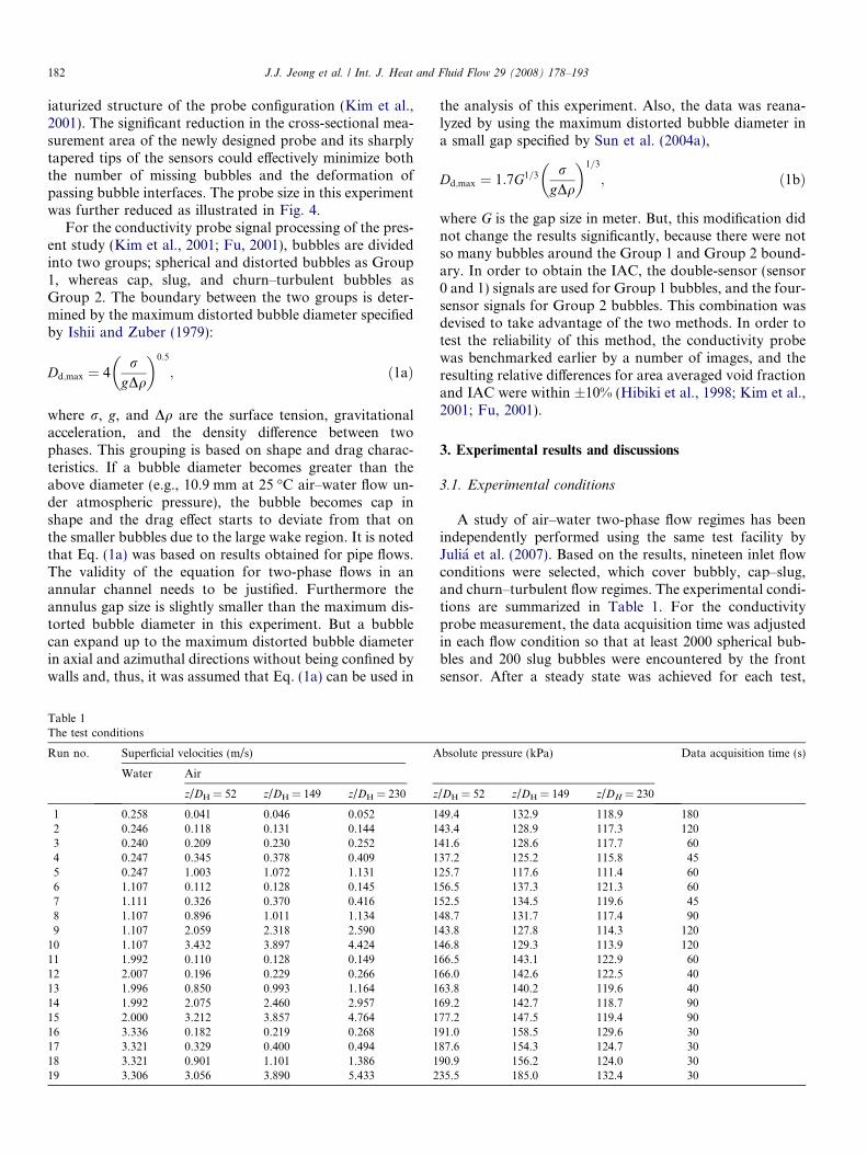
Table 1The test conditions

Run no. Superficial velocities (m/s) A

Water Air

z/DH = 52 z/DH = 149 z/DH = 230 z

1 0.258 0.041 0.046 0.052 12 0.246 0.118 0.131 0.144 13 0.240 0.209 0.230 0.252 14 0.247 0.345 0.378 0.409 15 0.247 1.003 1.072 1.131 16 1.107 0.112 0.128 0.145 17 1.111 0.326 0.370 0.416 18 1.107 0.896 1.011 1.134 19 1.107 2.059 2.318 2.590 1

10 1.107 3.432 3.897 4.424 111 1.992 0.110 0.128 0.149 112 2.007 0.196 0.229 0.266 113 1.996 0.850 0.993 1.164 114 1.992 2.075 2.460 2.957 115 2.000 3.212 3.857 4.764 116 3.336 0.182 0.219 0.268 117 3.321 0.329 0.400 0.494 118 3.321 0.901 1.101 1.386 119 3.306 3.056 3.890 5.433 2

the analysis of this experiment. Also, the data was reana-lyzed by using the maximum distorted bubble diameter ina small gap specified by Sun et al. (2004a),

Dd;max ¼ 1:7G1=3 rgDq

� �1=3

; ð1bÞ

where G is the gap size in meter. But, this modification didnot change the results significantly, because there were notso many bubbles around the Group 1 and Group 2 bound-ary. In order to obtain the IAC, the double-sensor (sensor0 and 1) signals are used for Group 1 bubbles, and the four-sensor signals for Group 2 bubbles. This combination wasdevised to take advantage of the two methods. In order totest the reliability of this method, the conductivity probewas benchmarked earlier by a number of images, and theresulting relative differences for area averaged void fractionand IAC were within ±10% (Hibiki et al., 1998; Kim et al.,2001; Fu, 2001).

3. Experimental results and discussions

3.1. Experimental conditions

A study of air–water two-phase flow regimes has beenindependently performed using the same test facility byJulia et al. (2007). Based on the results, nineteen inlet flowconditions were selected, which cover bubbly, cap–slug,and churn–turbulent flow regimes. The experimental condi-tions are summarized in Table 1. For the conductivityprobe measurement, the data acquisition time was adjustedin each flow condition so that at least 2000 spherical bub-bles and 200 slug bubbles were encountered by the frontsensor. After a steady state was achieved for each test,

bsolute pressure (kPa) Data acquisition time (s)

/DH = 52 z/DH = 149 z/DH = 230

49.4 132.9 118.9 18043.4 128.9 117.3 12041.6 128.6 117.7 6037.2 125.2 115.8 4525.7 117.6 111.4 6056.5 137.3 121.3 6052.5 134.5 119.6 4548.7 131.7 117.4 9043.8 127.8 114.3 12046.8 129.3 113.9 12066.5 143.1 122.9 6066.0 142.6 122.5 4063.8 140.2 119.6 4069.2 142.7 118.7 9077.2 147.5 119.4 9091.0 158.5 129.6 3087.6 154.3 124.7 3090.9 156.2 124.0 3035.5 185.0 132.4 30

100

101

Taitel et al. Bubbly to slug Bubbly to dispersed bubbly Dispersed bubbly to S/C

B S SB B BB B B S S S

S S SS S SB B SB B SB B B

SSC SS CBBSBBB

BBB CCCSCCBSSBBS

B B B

Mishima-Ishii Bubbly to slug Slug to churn turbulent

Sup

erfic

ial l

iqui

d ve

loct

y, j f (

m/s

)

z/DH=52

z/DH=149

z/DH=230

B: Bubbly S: Cap-slug C: Churn-turbulent

10-2 10-1 100 10110-2

10-1

100

101

-15 %

+15 %

Sup

erfic

ial g

as v

eloc

ity b

y pr

obe,

<j g>

[m/s

]

Superficial gas velocity by rotameter, <jg> [m/s]

z/DH=52

z/DH=149

z/DH=230

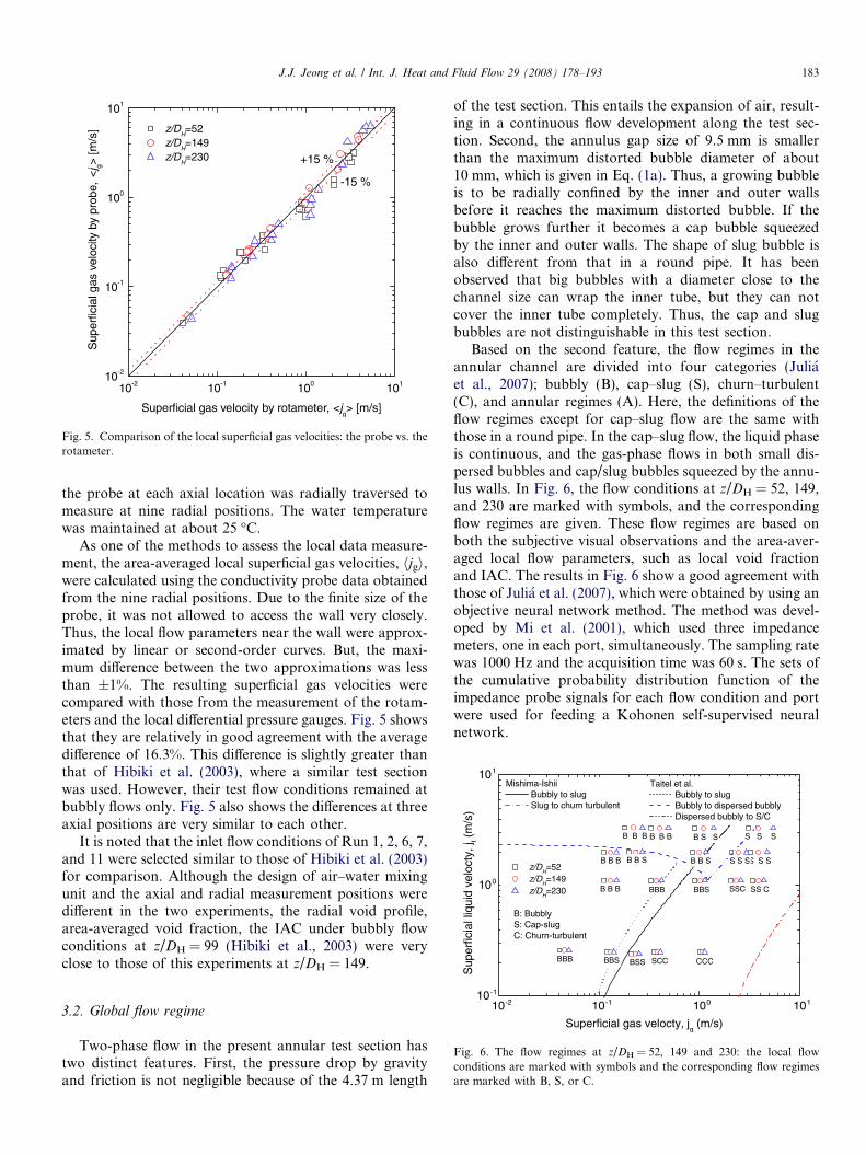
Fig. 5. Comparison of the local superficial gas velocities: the probe vs. therotameter.


the probe at each axial location was radially traversed tomeasure at nine radial positions. The water temperaturewas maintained at about 25 �C.

As one of the methods to assess the local data measure-ment, the area-averaged local superficial gas velocities, hjgi,were calculated using the conductivity probe data obtainedfrom the nine radial positions. Due to the finite size of theprobe, it was not allowed to access the wall very closely.Thus, the local flow parameters near the wall were approx-imated by linear or second-order curves. But, the maxi-mum difference between the two approximations was lessthan ±1%. The resulting superficial gas velocities werecompared with those from the measurement of the rotam-eters and the local differential pressure gauges. Fig. 5 showsthat they are relatively in good agreement with the averagedifference of 16.3%. This difference is slightly greater thanthat of Hibiki et al. (2003), where a similar test sectionwas used. However, their test flow conditions remained atbubbly flows only. Fig. 5 also shows the differences at threeaxial positions are very similar to each other.

It is noted that the inlet flow conditions of Run 1, 2, 6, 7,and 11 were selected similar to those of Hibiki et al. (2003)for comparison. Although the design of air–water mixingunit and the axial and radial measurement positions weredifferent in the two experiments, the radial void profile,area-averaged void fraction, the IAC under bubbly flowconditions at z/DH = 99 (Hibiki et al., 2003) were veryclose to those of this experiments at z/DH = 149.

10-2 10-1 100 10110-1

Superficial gas velocty, jg (m/s)

Fig. 6. The flow regimes at z/DH = 52, 149 and 230: the local flowconditions are marked with symbols and the corresponding flow regimesare marked with B, S, or C.

3.2. Global flow regime

Two-phase flow in the present annular test section hastwo distinct features. First, the pressure drop by gravityand friction is not negligible because of the 4.37 m length

of the test section. This entails the expansion of air, result-ing in a continuous flow development along the test sec-tion. Second, the annulus gap size of 9.5 mm is smallerthan the maximum distorted bubble diameter of about10 mm, which is given in Eq. (1a). Thus, a growing bubbleis to be radially confined by the inner and outer wallsbefore it reaches the maximum distorted bubble. If thebubble grows further it becomes a cap bubble squeezedby the inner and outer walls. The shape of slug bubble isalso different from that in a round pipe. It has beenobserved that big bubbles with a diameter close to thechannel size can wrap the inner tube, but they can notcover the inner tube completely. Thus, the cap and slugbubbles are not distinguishable in this test section.

Based on the second feature, the flow regimes in theannular channel are divided into four categories (Juliaet al., 2007); bubbly (B), cap–slug (S), churn–turbulent(C), and annular regimes (A). Here, the definitions of theflow regimes except for cap–slug flow are the same withthose in a round pipe. In the cap–slug flow, the liquid phaseis continuous, and the gas-phase flows in both small dis-persed bubbles and cap/slug bubbles squeezed by the annu-lus walls. In Fig. 6, the flow conditions at z/DH = 52, 149,and 230 are marked with symbols, and the correspondingflow regimes are given. These flow regimes are based onboth the subjective visual observations and the area-aver-aged local flow parameters, such as local void fractionand IAC. The results in Fig. 6 show a good agreement withthose of Julia et al. (2007), which were obtained by using anobjective neural network method. The method was devel-oped by Mi et al. (2001), which used three impedancemeters, one in each port, simultaneously. The sampling ratewas 1000 Hz and the acquisition time was 60 s. The sets ofthe cumulative probability distribution function of theimpedance probe signals for each flow condition and portwere used for feeding a Kohonen self-supervised neuralnetwork.


It can be seen in Fig. 6 that there are some entranceeffects in the flow-regime. For example, the flow at z/DH = 230 of Run 2 (hjfi = 0.25 m/s and hjgi = 0.14 m/s)was a slug flow whereas the flow at z/DH = 52 of Run 3(hjfi = 0.24 m/s and hjgi = 0.21 m/s) was a bubbly flow.Similarly, the flow at z/DH = 230 of Run 9 (hjfi = 1.11 m/s and hjgi = 2.59 m/s) was a churn–turbulent flow, butthe flow at z/DH = 52 of Run 10 (hjfi = 1.11 m/s andhjgi = 3.43) was a slug flow. This implies that a certain flowlength is needed for bubble growth and flow-regime evolu-tion, which clearly shows the limitation of static flow-regime maps and the necessity of the IAT approach, espe-cially for developing flows. However, the bubbly-to-slugtransition lines of Mishima and Ishii (1984) and Taitelet al. (1980), which were suggested for a flow in a roundpipe, predict the transition in the annulus reasonably well.

3.3. Local flow structure

The local flow structure is mainly determined by bubblecoalescence and breakup. The mechanism of bubble inter-actions can be summarized in five categories (Ishii andHibiki, 2006): the coalescence due to random collisions dri-ven by liquid turbulence; the coalescence due to wakeentrainment, the breakup due to the impact of turbulenteddies, the shearing-off of small bubbles from cap/slugbubbles; and the breakup of large cap bubbles due to sur-face instability. Relative importance of these terms dependson flow conditions.

The radial migration of bubbles also plays an importantrole in the evolution of local flow structure. Zun (1988)studied transition from wall void peaking to core voidpeaking in turbulent bubbly flow in terms of bubble size,and suggested critical bubble sizes between the wall – inter-mediate – core void peaks. Tomiyama et al. (2002), Prasseret al. (2002), Lucas et al. (2005), and Krepper et al. (2005)also showed that small bubbles tend to move toward thewall, whereas large bubbles greater than 5.1–5.5 mmtoward the center of the channel because the direction ofthe lift force is dependent on the bubble size. This resultsin the radial separation of small and large bubbles. Thisagain affects the bubble interactions because they are radi-ally not uniform but more active near the wall due to thehigher turbulent intensity.

Figs. 7 and 8 show the radial distributions of time-aver-aged local void fraction and IAC at z/DH = 149 for thenineteen conditions, respectively. In the sub-figures of Figs.7 and 8, hjgi increases from left to right, and hjfi increasesfrom bottom to top. These figures show global effects ofhjgi and hjfi on local flow structures. By increasing hjgi, voidfraction increases, i.e., the bubble density increases. Thisresults in an increase in the bubble coalescence rate. Ifsome bubbles become sufficiently large, they move towardthe center of the annulus gap. Because of the low turbulentkinetic energy at the center, they have a less probability ofbreakup and can grow further by coalescence due to ran-dom collisions and wake entrainment. This mechanism is

the key for the transition from bubbly-to-slug flow (Krep-per et al., 2005). Meanwhile, by increasing hjfi, the dissipa-tion rate of turbulent energy increases and, as a result, thefrequency of bubble breakup increases. This generatessmall bubbles and, thus, the wall or intermediate peakingof void fraction.

For the tests under bubbly flows, the void fraction pro-files of Run 1 and 2 have a center peak and the others havean intermediate peak. As mentioned earlier, the bubblediameter has a strong influence on the void fraction profile,and it is affected by the liquid velocity, which will be dis-cussed later. Thus, for fully developed flows, the void frac-tion profile can be given in a map of hjfi � hjgi plane.Serizawa and Kataoka (1988) suggested a simple modelfor phase distribution patterns in a vertical round pipe.Since their model was developed from fully developedflows, the evolution of bubble size was not taken intoaccount. Lucas et al. (2005) also showed z/DH-dependentphase distribution pattern maps, which were developedfrom the bubbly/slug flow data in a vertical pipe with aninner diameter of 51.2 mm and a length of 3 m. The trendof void fraction profiles in Fig. 7 is consistent with that ofby Lucas et al. (2005) at z/DH = 59.

The IAC, ai, for a bubbly flow can be given by

ai ¼ 6ag

DS

ð2Þ

where ag is the void fraction and DS is the Sauter meandiameter. Therefore, the radial profiles of void fractionand IAC are very similar if DS is radially uniform. How-ever, the radial profile of DS of Group 1 bubble alwayshas a broad center peak (e.g., see Fig. 12). This yields agreater peak-to-average ratio in the measured IAC profileas can be seen in Fig. 8, if the void fraction profile is wallor intermediate peaked.

As shown in Figs. 7 and 8, the slug flows are character-ized by high void fraction and low IAC, where the voidfraction is center-peaked and the IAC is wall-peaked. Thistrend is getting more clear in the churn–turbulent flowregimes.

Table 2 shows the effect of hjgi on the bubble count rateand the flow-regime at a constant hjfi of 1.11 m/s. The bub-ble count rate means the area-averaged number of bubblesthat were counted by the conductivity probe at the nineradial locations during one second. At low hjgi conditions,the Group 1 bubble number increases along the channeldue to the bubble breakup. However, when hjgi reaches0.90 m/s, coalescence occurs between z/DH = 149 and230. This results in a decrease of Group 1 bubbles andan increase of Group 2 bubbles, that is, a transition occursfrom bubbly-to-slug flow. It can be seen that a significantnumber of Group 1 bubbles are agglomerated into Group2 bubbles at slug flows of Run 9 and 10. If hjgi is increasedfurther, a flow transition occurs from slug to churn–turbu-lent flow. The transitions were not discrete but smoothuntil a certain flow condition.

0.0 0.2 0.4 0.6 0.8 1.00

20

40

60

80

100

Run 19<j

f>=3.31 m/s

<jg>=3.89 m/s

Run 18<j

f>=3.32 m/s

<jg>=1.10 m/s

Run 17<j

f>=3.32 m/s

<jg>=0.40 m/s

Run 16<j

f>=3.34 m/s

<jg>=0.22 m/s

Tim

e-av

erag

ed v

oid

frac

tion,

[%

]

To tal Group 1 Group 2

0.0 0.2 0.4 0.6 0.8 1.0 0.0 0.2 0.4 0.6 0.8 1.0 0.0 0.2 0.4 0.6 0.8 1.0

0.0 0.2 0.4 0.6 0.8 1.00

20

40

60

80

100

Run 15<j

f>=2.00 m/s

<jg>=3.86 m/s

Run 14<j

f>=1.99 m/s

<jg>=2.46 m/s

Run 13<j

f>=2.00 m/s

<jg>=0.99 m/s

Run 12<j

f>=2.01 m/s

<jg>=0.23 m/s

Run 11<j

f>=1.99 m/s

<jg>=0.13 m/s

Tim

e-av

erag

ed v

oid

frac

tion,

[%

]

Total Group 1 Group 2

0.0 0.2 0.4 0.6 0.8 1.0 0.0 0.2 0.4 0.6 0.8 1.0 0.0 0.2 0.4 0.6 0.8 1.0 0.0 0.2 0.4 0.6 0.8 1.0

0.0 0.2 0.4 0.6 0.8 1.00

20

40

60

80

100Run 10<j

f>=1.11 m/s

<jg>=3.90 m/s

Run 9<j

f>=1.11 m/s

<jg>=2.32 m/s

Run 8<j

f>=1.11 m/s

<jg>=1.01 m/s

Run 7<j

f>=1.11 m/s

<jg>=0.37 m/s

Run 6<j

f>=1.11 m/s

<jg>=0.13 m/s

Tim

e-av

erag

ed v

oid

frac

tion,

[%

]


0.0 0.2 0.4 0.6 0.8 1.0 0.0 0.2 0.4 0.6 0.8 1.0 0.0 0.2 0.4 0.6 0.8 1.0 0.0 0.2 0.4 0.6 0.8 1.0

0.0 0.2 0.4 0.6 0.8 1.00

20

40

60

80

100

Run 5<j

f>=0.25 m/s

<jg>=1.07 m/s

Run 4<j

f>=0.25 m/s

<jg>=0.38 m/s

Run 3<j

f>=0.24 m/s

<jg>=0.23 m/s

Run 2<j

f>=0.25 m/s

<jg>=0.13 m/s

Run 1<j

f>=0.26 m/s

<jg>=0.05 m/s

Tim

e-av

erag

ed v

oid

frac

tion,

[%

]

Radial position, (r-Ri)/(R

o-R

i) [-]


0.0 0.2 0.4 0.6 0.8 1.0 0.0 0.2 0.4 0.6 0.8 1.0 0.0 0.2 0.4 0.6 0.8 1.0 0.0 0.2 0.4 0.6 0.8 1.0

Fig. 7. Radial distributions of time-averaged void fraction at z/DH = 149.


The effect of increasing hjfi is clearly shown in the resultsof Run 16 (hjfi = 3.34 m/s and hjgi = 0.18 m/s at z/DH =

52). In Run 16, the flow regimes in the whole test sectionremained at bubbly flow and the average DS of Group 1

0.0 0.2 0.4 0.6 0.8 1.00

300

600

900

1200

1500

Run 19<j

f>=3.31 m/s

<jg>=3.89 m/s

Run 18<j

f>=3.32 m/s

<jg>=1.10 m/s

Run 17<j

f>=3.32 m/s

<jg>=0.40 m/s

Run 16<j

f>=3.34 m/s

<jg>=0.22 m/s

Tim

e-av

erag

ed IA

C, a

i [m

-1]


0.0 0.2 0.4 0.6 0.8 1.0 0.0 0.2 0.4 0.6 0.8 1.0 0.0 0.2 0.4 0.6 0.8 1.0

0.0 0.2 0.4 0.6 0.8 1.00

300

600

900

1200

1500

Run 15<j

f>=2.00 m/s

<jg>=3.86 m/s

Run 14<j

f>=1.99 m/s

<jg>=2.46 m/s

Run 13<j

f>=2.00 m/s

<jg>=0.99 m/s

Run 12<j

f>=2.01 m/s

<jg>=0.23 m/s

Run 11<j

f>=1.99 m/s

<jg>=0.13 m/s

Tim

e-av

erag

ed IA

C, a

i [m

-1]


0.0 0.2 0.4 0.6 0.8 1.0 0.0 0.2 0.4 0.6 0.8 1.0 0.0 0.2 0.4 0.6 0.8 1.0 0.0 0.2 0.4 0.6 0.8 1.0

0.0 0.2 0.4 0.6 0.8 1.00

300

600

900

1200

1500

Run 10<j

f>=1.11 m/s

<jg>=3.90 m/s

Run 9<j

f>=1.11 m/s

<jg>=2.32 m/s

Run 8<j

f>=1.11 m/s

<jg>=1.01 m/s

Run 7<j

f>=1.11 m/s

<jg>=0.37 m/s

Run 6<j

f>=1.11 m/s

<jg>=0.13 m/s

Tim

e-av

erag

ed IA

C, a

i [m

-1]


0.0 0.2 0.4 0.6 0.8 1.0 0.0 0.2 0.4 0.6 0.8 1.0 0.0 0.2 0.4 0.6 0.8 1.0 0.0 0.2 0.4 0.6 0.8 1.0

0.0 0.2 0.4 0.6 0.8 1.00

300

600

900

1200

1500

Run 5<j

f>=0.25 m/s

<jg>=1.07 m/s

Run 4<j

f>=0.25 m/s

<jg>=0.38 m/s

Run 3<j

f>=0.24 m/s

<jg>=0.23 m/s

Run 2<j

f>=0.25 m/s

<jg>=0.13 m/s

Run 1<j

f>=0.26 m/s

<jg>=0.05 m/s

Tim

e-av

erag

ed IA

C, a

i [m

-1]


o-R

i) [-]


0.0 0.2 0.4 0.6 0.8 1.0 0.0 0.2 0.4 0.6 0.8 1.0 0.0 0.2 0.4 0.6 0.8 1.0 0.0 0.2 0.4 0.6 0.8 1.0

Fig. 8. Radial distributions of time-averaged IAC at z/DH = 149.


bubbles were 1.6 mm. The radial void profiles of Run 16 atthe three measurement ports are shown in Fig. 9a. They are

intermediate peaked and the average void fraction slightlyincreases along the flow channel due to the expansion.

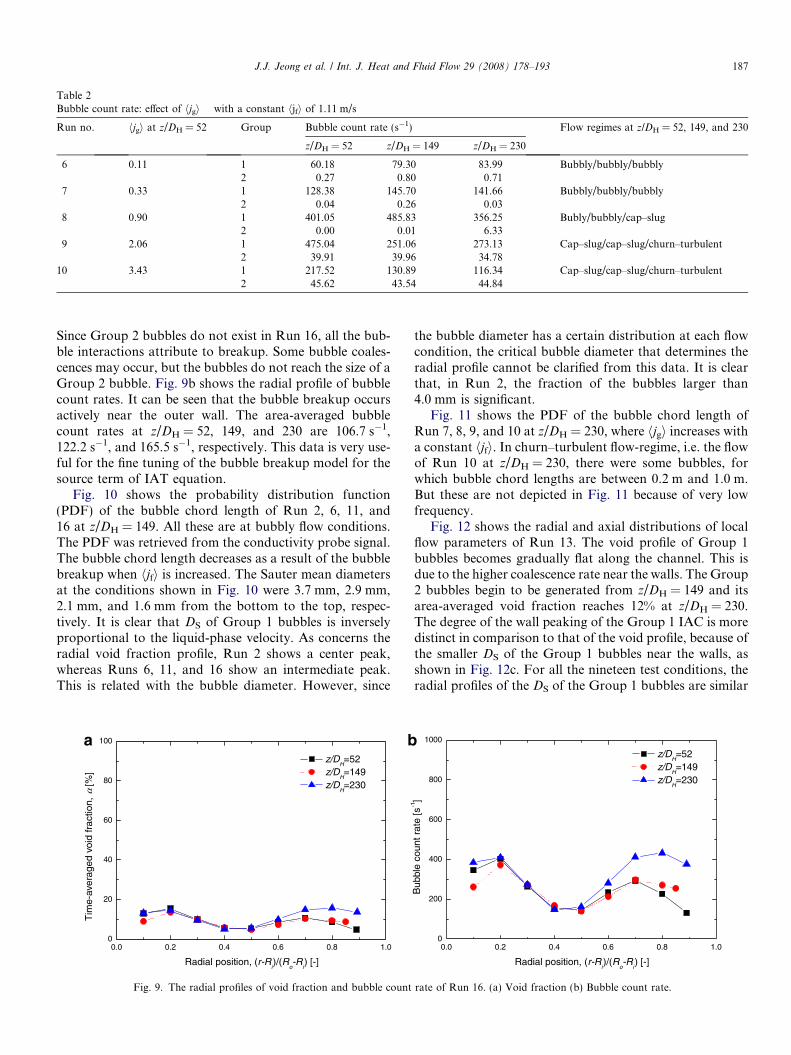
Table 2Bubble count rate: effect of hjgi with a constant hjfi of 1.11 m/s

Run no. hjgi at z/DH = 52 Group Bubble count rate (s�1) Flow regimes at z/DH = 52, 149, and 230

z/DH = 52 z/DH = 149 z/DH = 230

6 0.11 1 60.18 79.30 83.99 Bubbly/bubbly/bubbly2 0.27 0.80 0.71

7 0.33 1 128.38 145.70 141.66 Bubbly/bubbly/bubbly2 0.04 0.26 0.03

8 0.90 1 401.05 485.83 356.25 Bubly/bubbly/cap–slug2 0.00 0.01 6.33

9 2.06 1 475.04 251.06 273.13 Cap–slug/cap–slug/churn–turbulent2 39.91 39.96 34.78

10 3.43 1 217.52 130.89 116.34 Cap–slug/cap–slug/churn–turbulent2 45.62 43.54 44.84


Since Group 2 bubbles do not exist in Run 16, all the bub-ble interactions attribute to breakup. Some bubble coales-cences may occur, but the bubbles do not reach the size of aGroup 2 bubble. Fig. 9b shows the radial profile of bubblecount rates. It can be seen that the bubble breakup occursactively near the outer wall. The area-averaged bubblecount rates at z/DH = 52, 149, and 230 are 106.7 s�1,122.2 s�1, and 165.5 s�1, respectively. This data is very use-ful for the fine tuning of the bubble breakup model for thesource term of IAT equation.

Fig. 10 shows the probability distribution function(PDF) of the bubble chord length of Run 2, 6, 11, and16 at z/DH = 149. All these are at bubbly flow conditions.The PDF was retrieved from the conductivity probe signal.The bubble chord length decreases as a result of the bubblebreakup when hjfi is increased. The Sauter mean diametersat the conditions shown in Fig. 10 were 3.7 mm, 2.9 mm,2.1 mm, and 1.6 mm from the bottom to the top, respec-tively. It is clear that DS of Group 1 bubbles is inverselyproportional to the liquid-phase velocity. As concerns theradial void fraction profile, Run 2 shows a center peak,whereas Runs 6, 11, and 16 show an intermediate peak.This is related with the bubble diameter. However, since

0.0 0.2 0.4 0.6 0.8 1.00

20

40

60

80

100

z/DH=52

z/DH=149

z/DH=230

Tim

e-av

erag

ed v

oid

frac

tion,

α [%

]


o-R

i) [-]

a b

Fig. 9. The radial profiles of void fraction and bubble count

the bubble diameter has a certain distribution at each flowcondition, the critical bubble diameter that determines theradial profile cannot be clarified from this data. It is clearthat, in Run 2, the fraction of the bubbles larger than4.0 mm is significant.

Fig. 11 shows the PDF of the bubble chord length ofRun 7, 8, 9, and 10 at z/DH = 230, where hjgi increases witha constant hjfi. In churn–turbulent flow-regime, i.e. the flowof Run 10 at z/DH = 230, there were some bubbles, forwhich bubble chord lengths are between 0.2 m and 1.0 m.But these are not depicted in Fig. 11 because of very lowfrequency.

Fig. 12 shows the radial and axial distributions of localflow parameters of Run 13. The void profile of Group 1bubbles becomes gradually flat along the channel. This isdue to the higher coalescence rate near the walls. The Group2 bubbles begin to be generated from z/DH = 149 and itsarea-averaged void fraction reaches 12% at z/DH = 230.The degree of the wall peaking of the Group 1 IAC is moredistinct in comparison to that of the void profile, because ofthe smaller DS of the Group 1 bubbles near the walls, asshown in Fig. 12c. For all the nineteen test conditions, theradial profiles of the DS of the Group 1 bubbles are similar

0.0 0.2 0.4 0.6 0.8 1.00

200

400

600

800

1000

Bub

ble

coun

t rat

e [s

-1]


o-R

i) [-]

z/DH=52

z/DH=149

z/DH=230

rate of Run 16. (a) Void fraction (b) Bubble count rate.

0.00 0.04 0.08 0.12 0.16 0.2010-3

10-2

10-1

100

PD

F o

f Cho

rd le

ngth

[m-1]

Chord length [m]

Run 7:<j

f>=1.11 m/s, <j

g>=0.42 m/s

10-3

10-2

10-1

100

Run 8:<j

f>=1.11 m/s, <j

g>=1.13 m/s

PD

F o

f Cho

rd le

ngth

[m-1]

10-3

10-2

10-1

100

Run 9:<j

f>=1.11 m/s, <j

g>=2.59 m/s

PD

F o

f Cho

rd le

ngth

[m-1]

10-3

10-2

10-1

100

Run 10:<j

f>=1.11 m/s, <j

g>=4.42 m/s

PD

F o

f Cho

rd le

ngth

[m-1]

Fig. 11. The PDFs of the chord length of Run 7, 8, 9, and 10 at (r � Ri)/(R0 � Ri) = 0.7 and z/DH = 230.

0.000 0.002 0.004 0.006 0.008 0.0100.00

0.05

0.10

0.15

0.20

PD

F o

f Cho

rd le

ngth

[m-1]

Chord length [m]

Run 2:<j

f>=0.25 m/s, <j

g>=0.13 m/s

0.00

0.05

0.10

0.15

0.20

Run 6:<j

f>=1.11 m/s, <j

g>=0.13 m/s

PD

F o

f Cho

rd le

ngth

[m-1]

0.00

0.05

0.10

0.15

0.20

Run 11:<j

f>=1.99 m/s, <j

g>=0.13 m/s

PD

F o

f Cho

rd le

ngth

[m-1]

0.00

0.05

0.10

0.15

0.20

Run 16:<j

f>=3.34 m/s, <j

g>=0.22 m/s

PD

F o

f Cho

rd le

ngth

[m-1]

Fig. 10. The PDFs of the chord length of Run 2, 6, 11, and 16 at (r � Ri)/(R0 � Ri) = 0.7 and z/DH = 149.


to that in Fig. 12c, showing a broad center peak. Thisimplies that the large bubbles tend to move toward thecenter. Fig. 12c also shows the average chord lengths ofGroup 2 bubbles, which become longer along the channeldue to the bubble coalescence.

The interfacial velocity profiles at the three axial loca-tions are shown in Fig. 12d and they are very similar to thatof turbulent single-phase liquid flow (Quadrio and Luchini,2002). Because of the finite size of the probe, the velocitiesnear the walls could not be measured. Each velocity inFig. 12d is the average of the interface velocities of allthe bubbles that hit the conductivity probe. The standarddeviation of the velocity fluctuation at z/DH = 230 was26.6%. The area-averaged velocity of Group 1 bubblesslightly increases along the channel.

It can be seen, from Figs 7–12 and Table 2, that the evo-lution of local flow structure is smooth to a certain extentand, for a given flow condition, the flow regime is deter-

mined by the degree of the progress toward an equilibriumpoint, which is balanced by bubble coalescence, breakup,and radial migration.

3.4. Axial evolution of the flow structure and interfacial area

transport

Fig. 13 shows the axial profiles of the area-averaged voidfraction. The steady-state one-dimensional continuityequation of the gas phase is given by

d

dzðhagiqghhvgiiÞ ¼ 0; ð3Þ

or

1

hagid

dzhagi þ

1

qg

d

dzqg þ

1

hhvgiid

dzhhvgii ¼ 0; ð4Þ

0.0 0.2 0.4 0.6 0.8 1.00

20

40

60

80

100

Group 2z/D

H=52

z/DH=149

z/DH=230

Group 1z/D

H=52

z/DH=149

z/DH=230

Tim

e-av

erag

ed v

oid

frac

tion,

α [%

]


o-R

i) [-]

0.0 0.2 0.4 0.6 0.8 1.00

400

800

1200

1600

2000

Group 1z/D

H=52

z/DH

=149z/D

H=230

Group 2z/D

H=52

z/DH=149

z/DH=230

Tim

e-av

erag

ed I

AC

, a i [

m-1]


o-R

i) [-]

0.0 0.2 0.4 0.6 0.8 1.00.00

0.01

0.02

0.03

0.04

0.05

DSM

of Group 1z/D

H=52

z/DH=149

z/DH=230

ACL of Group 2z/D

H=52

z/DH=149

z/DH=230

DS o

r A

CL

[m]


o-R

i) [-]

0.0 0.2 0.4 0.6 0.8 1.00

1

2

3

4

5

Group 2z/D

H=52

z/DH

=149z/D

H=230

Group 1z/D

H=52

z/DH=149

z/DH=230

Inte

rfac

ial v

eloc

ity,

v i [m

/s]


o-R

i) [-]

a b

c d

Fig. 12. The radial and axial distributions of local flow parameters of Run 13. (a) Void fraction (b) IAC (c) DS or average chord length (ACL) (d)Interfacial velocity.


where hagi, qg, and hhvgii are area-averaged void fraction,density, and void-weighted area-averaged velocity, respec-tively. Using the ideal gas law for gas density, Eq. (4) is rep-resented by

1

hagid

dzhagi ¼ �

1

Pd

dzP � 1

hhvgiid

dzhhvgii ð5Þ

where P is pressure. The first term in the right-hand side(RHS) of Eq. (5) is always positive and it increases as thetotal mass flow rate increases. The second term in theRHS of Eq. (5) can be either positive or negative, but itseffect decreases as the gas-phase velocity increases. As awhole, the area-averaged void fraction is expected to in-crease along the flow channel with the increase of totalmass flow rate and/or gas-phase velocity. This trend canbe seen in Fig. 13.

The axial profiles of area-averaged IAC are compared inFig. 14. By considering the IAC data at z/DH = 52 asboundary conditions, the data at z/DH = 149 and 230 canbe used for the development and assessment of IAT mod-els. The cap–slug and churn–turbulent flows are character-

ized by a high void fraction and a low IAC. In general,because the contribution of Group 1 bubbles is dominantto total IAC, the total IAC is nearly proportional to thevoid fraction of Group 1 bubbles. This can be confirmedby comparing Figs. 13 and 14. However, the results ofRun 18 with hjfi = 3.32 m/s are somewhat interesting.Fig. 13 shows the void fraction of Group 1 bubbles ofRun 18 decreases and that of Group 2 increases alongthe flow channel, which means that there is bubble coales-cence. However, in spite of the decrease of Group 1 bubblevoid fraction, the IAC of Group 1 bubbles increasesbecause of the bubble breakup. This means both bubblecoalescence and breakup occurred actively between z/DH = 149 and 230.

4. Conclusions

An experimental study on the IAT of vertical, upward,air–water two-phase flows in an annulus channel has beenperformed. The inner and outer diameters of the annulusare 19.1 mm and 38.1 mm, respectively. Nineteen inlet flow

0 100 200 3000

20

40

60

80

100

Run 19<j

f>=3.31 m/s

<jg>=3.06 m/s

Run 18<j

f>=3.32 m/s

<jg>=0.90 m/s

Run 17<j

f>=3.32 m/s

<jg>=0.33 m/s

Run 16<j

f>=3.34 m/s

<jg>=0.18 m/s

Are

a-av

erag

ed v

oid

frac

tion,

<α

> [%

]


0 100 200 300 0 100 200 300 0 100 200 300

0 100 200 3000

20

40

60

80

100

Run 15<j

f>=2.00 m/s

<jg>=3.21 m/s

Run 14<j

f>=1.99 m/s

<jg>=2.08m/s

Run 13<j

f>=2.00 m/s

<jg>=0.85 m/s

Run 12<j

f>=2.01 m/s

<jg>=0.20 m/s

Run 11<j

f>=1.99 m/s

<jg>=0.11 m/s

Are

a-av

erag

ed v

oid

frac

tion,

<α

> [%

]


0 100 200 300 0 100 200 300 0 100 200 300 0 100 200 300

0 100 200 3000

20

40

60

80

100

Run 10<j

f>=1.11 m/s

<jg>=3.43 m/s

Run 9<j

f>=1.11 m/s

<jg>=2.06 m/s

Run 8<j

f>=1.11 m/s

<jg>=0.90 m/s

Run 7<j

f>=1.11 m/s

<jg>=0.33 m/s

Run 6<j

f>=1.11 m/s

<jg>=0.11 m/s

Are

a-av

erag

ed v

oid

frac

tion,

<α

> [%

]


0 100 200 300 0 100 200 300 0 100 200 300 0 100 200 300

0 100 2000

20

40

60

80

100

Run 5<j

f>=0.25 m/s

<jg>=1.00 m/s

Run 4<j

f>=0.25 m/s

<jg>=0.35 m/s

Run 3<j

f>=0.24 m/s

<jg>=0.21 m/s

Run 2<j

f>=0.25 m/s

<jg>=0.12 m/s

Run 1<j

f>=0.26 m/s

<jg>=0.04 m/s

Are

a-av

erag

ed v

oid

frac

tion,

<α

> [%

]

Axial position, z/DH [-]


0 100 200 300 0 100 200 300 0 100 200 300 0 100 200 300300

Fig. 13. Axial profiles of area-averaged void fraction: the flow conditions at z/DH = 52 are given.


conditions were selected so that a wide range of flow con-ditions could be covered, including bubbly, cap–slug, and

churn–turbulent flows. Using the four-sensor conductivityprobes, the local flow parameters were measured at nine

0 100 200 3000

300

600

900

1200

1500

Run 19<j

f >=3.31 m/s<j

g>=3.06 m/s

Run 18<j

f >=3.32 m/s<j

g>=0.90 m/s

Run 17<j

f>=3.32 m/s

<jg>=0.33 m/s

Run 16<j

f>=3.34 m/s

<jg>=0.18 m/s

Are

a-av

erag

ed IA

C, <

a i> [m

-1]


0 100 200 300 0 100 200 300 0 100 200 300

0 100 200 3000

300

600

900

1200

1500Run 15<j

f>=2.00 m/s

<jg>=3.21 m/s

Run 14<j

f>=1.99 m/s

<jg>=2.08m/s

Run 13<j

f>=2.00 m/s

<jg>=0.85 m/s

Run 12<j

f>=2.01 m/s

<jg>=0.20 m/s

Run 11<j

f>=1.99 m/s

<jg>=0.11 m/s

Are

a-av

erag

ed IA

C, <

a i> [m

-1]


0 100 200 300 0 100 200 300 0 100 200 300 0 100 200 300

0 100 200 3000

300

600

900

1200

1500

Run 10<j

f>=1.11 m/s

<jg>=3.43 m/s

Run 9<j

f>=1.11 m/s

<jg>=2.06 m/s

Run 8<j

f>=1.11 m/s

<jg>=0.90 m/s

Run 7<j

f>=1.11 m/s

<jg>=0.33 m/s

Run 6<j

f>=1.11 m/s

<jg>=0.11 m/s

Are

a-av

erag

ed IA

C, <

a i> [m

-1]


0 100 200 300 0 100 200 300 0 100 200 300 0 100 200 300

0 100 200 3000

300

600

900

1200

1500

Run 5<j

f>=0.25 m/s

<jg>=1.00 m/s

Run 4<j

f>=0.25 m/s

<jg>=0.35 m/s

Run 3<j

f>=0.24 m/s

<jg>=0.21 m/s

Run 2<j

f>=0.25 m/s

<jg>=0.12 m/s

Run 1<j

f>=0.26 m/s

<jg>=0.04 m/s

Are

a-av

erag

ed IA

C, <

a i> [ m

-1]

Axial position, z/DH [-]


0 100 200 300 0 100 200 300 0 100 200 300 0 100 200 300

Fig. 14. Axial profiles of area-averaged IAC: the flow conditions at z/DH = 52 are given.


radial positions for the three axial locations (z/DH = 52,149 and 230). The data include local void fractions, interfa-

cial area concentrations, interfacial velocities, and bubblecount rates for the two groups of bubbles.


Using the data for the nineteen conditions, the effectsof hjgi, hjfi, and z/DH on the local flow structure wereanalyzed. The data clearly showed the limitation of thestatic flow-regime maps and the necessity of the IATapproach, especially for developing flows. The effect ofbubble diameter was also discussed and it was shown thatsmall bubbles tend to move to the wall, and large bubblesto the center. Using the local bubble count rate, theradial and axial evolutions of IAC were interpreted interms of bubble coalescence and breakup. Since the con-tribution of Group 1 bubbles to total IAC is dominant,the total IAC is nearly proportional to the void fractionof Group 1 bubbles. The slug and churn–turbulent flowswere characterized by high void fraction and low IAC,where the void fraction is center-peaked and the IAC iswall-peaked. Even though this is obvious in the literature,very limited data supporting this fact quantitatively areavailable.

The measured data would be very useful for the develop-ment of the two-group IAT model, especially for the bub-ble coalescence and breakup models. Some of the data canbe used for the fine tuning of individual source and sinkterms of IAT equations. The data would be also suitablefor the development of some closure models for computa-tional fluid dynamics.

Acknowledgements

One of the coauthors, J.J. Jeong, would like to thankSchool of Nuclear Engineering, Purdue University. Thiswork has been performed during his sabbatical leave atPurdue University under the financial support from KoreaAtomic Energy Research Institute.

References

Bestion, D., 1990. The physical closure laws in the CATHARE code.Nucl. Eng. Design 124, 229–345.

Das, G., Das, P.K., Purohit, N.K., Mitra, A.K., 1999. Flow patterntransition during gas liquid upflow through vertical concentric annuli –Part I: experimental investigations. J. Fluids Eng. 121, 895–901.

Fu, X., 2001. Interfacial Area Measurement and Transport Modeling inAir–water Two-phase Flow, PhD Thesis, Purdue University, WestLafayette, Indiana, USA.

Grosstete, G., 1995. Experimental Investigation and preliminary numer-ical simulations of void profile development in a vertical cylindricalpipe. In: Second International Conference on Multiphase Flow,Tokyo, Japan, April 3–7, 1995.

Hibiki, T., Ishii, M., 1999. Experimental study on interfacial areatransport in bubbly two-phase flows. Int. J. Heat Mass Transfer 42,3019–3035.

Hibiki, T., Ishii, M., 2000. One-group interfacial area transport of bubblyflows in vertical round tubes. Int. J. Heat Mass Transfer 43, 2711–2726.

Hibiki, T., Hogsett, S., Ishii, M., 1998. Local measurement of interfacialarea, interfacial velocity and liquid turbulence in two-phase flow. Nucl.Eng. Design 184, 287–304.

Hibiki, T., Takamasa, T., Ishii, M., 2001. Interfacial area transport ofbubbly flow in a small diameter pipe. J. Nucl. Sci. Technol. 38, 614–620.

Hibiki, T., Mi, Y., Situ, R., Ishii, M., 2003. Interfacial area transport ofvertical upward bubbly two-phase flow in an annulus. Int. J. HeatMass Transfer 46, 4949–4962.

Ishii, M., 1975. Thermo-fluid Dynamic Theory of Two-phase Flow,Collection de la Direction den Etudes et Researches d’Electricite deFrance, Eyrolles, Paris, France, pp. 176–179.

Ishii, M., Hibiki, T., 2006. Thermo-fluid Dynamics of Two-phase Flow.Springer, New York, USA.

Ishii, M., Kim, S., 2001. Micro four-sensor probe measurement ofinterfacial area transport for bubbly flow in round pipes. Nucl. Eng.Design 205, 123–131.

Ishii, M., Kim, S., 2004. Development of one-group and two-groupinterfacial area transport equation. Nucl. Sci. Eng. 146 (3), 257–273.

Ishii, M., Zuber, N., 1979. Drag coefficient and relative velocity in bubbly,droplet or particulate flows. AIChE J. 25, 843–855.

Ishii, M., Kim, S., Kelly, J., 2005. Development of interfacial areatransport equation. Nucl. Eng. Technol. 37, 525–536.

Julia, J.E., Jeong, J.J., Dixit, A., Ozar, B., Hibiki, T., Ishii, M., 2007. Flowregime identification and analysis in adiabatic upward two-phase flowin an annulus geometry. In: 15th International Conference on NuclearEngineering, Nagoya, Japan, April 22–26, 2007.

Kataoka, I., Ishii, M., Serizawa, A., 1986. Local formulation andmeasurement of interfacial area concentration in two-phase flow. Int.J. Multiphase Flow 12, 505–529.

Kelessidis, V.C., Dukler, A.E., 1989. Modelling flow pattern transitionsfor upward gas–liquid flow in vertical concentric and eccentric annuli.Int. J. Multiphase Flow 15, 173–191.

Kim, S., Fu, X., Wang, X., Ishii, M., 2000. Development of theminiaturized four-sensor conductivity probe and the signal processingscheme. Int. J. Heat Mass Transfer 43, 4101–4118.

Kim, S., Fu, X., Wang, X., Ishii, M., 2001. Study on interfacial structuresin slug flows using a miniaturized four-sensor conductivity probe.Nucl. Eng. Design 204, 45–55.

Kocamustafaogullari, G., Ishii, M., 1995. Foundation of the interracialarea transport equation and its closure relations. Int. J. Heat MassTransfer 38 (3), 481–493.

Krepper, E., Lucas, D., Prasser, H.-M., 2005. On the modelling of bubblyflow in vertical pipes. Nucl. Eng. Design 235, 597–611.

Lucas, D., Krepper, E., Prasser, H.-M., 2005. Development of co-currentair–water flow in a vertical pipe. Int. J. Multiphase Flow 31, 1304–1328.

Matijevic, E., 1969. Surface and Colloid Science. Wiley-Interscience, NewYork.

Mi, Y., Ishii, M., Tsoukalas, L.H., 2001. Flow regime identificationmethodology with neural networks and two-phase flow models. Nucl.Eng. Design 204, 87–100.

Mishima, K., Ishii, M., 1984. Flow regime transition criteria for upwardtwo-phase flow in vertical tubes. Int. J. Heat Mass Transfer 27 (5),723–737.

Morel, C., Goreaud, N., Delhaye, J.M., 1999. The local volumetricinterfacial area transport equation: derivation and physical signifi-cance. Int. J. Multiphase Flow 25, 1099–1128.

Neal, L.G., Bankoff, S.G., 1963. A high resolution resistivity probe fordetermination of local void properties in gas–liquid flow. AIChE J. 9,490–494.

Prasser, H.-M., Krepper, E., Lucas, D., 2002. Evolution of the two-phaseflow in a vertical tube—decomposition of gas fraction profilesaccording to bubble size classes using wire-mesh sensors. Int. J.Therm. Sci. 41, 17–28.

Quadrio, M., Luchini, P., 2002. Direct numerical simulation of theturbulent flow in a pipe with annular cross section. Eur. J. Mech. B –Fluids 21, 413–427.

Revankar, S.T., Ishii, M., 1992. Local interfacial area measurement inbubbly flow. Int. J. Heat Mass Transfer 35, 913–925.

Revankar, S.T., Ishii, M., 1993. Theory and measurement of localinterfacial area using a four sensor probe in two-phase flow. Int. J.Heat Mass Transfer 36, 2997–3007.


SCIENTECH, Inc., 1998. RELAP5/MOD3 Code Manual Volume I: codestructure, system models and solution methods. Formerly NUREG/CR-5535. U.S. Nuclear Regulatory Commission.

Serizawa, A., Kataoka, I., 1988. Phase distribution in two-phase flow. In:Afgan, N.H. (Ed.), Transient Phenomena in Multi Phase Flow.Hemisphere, Washington DC, pp. 179–224.

Situ, R., Hibiki, T., Sun, X., Mi, Y., Ishii, M., 2004. Flow structure ofsubcooled boiling flow in an internally heated annulus. Int. J. HeatMass Transfer 47, 5351–5364.

Smith, T.R., 2002, Two-group Interfacial Area Transport Equation inLarge Diameter Pipes, PhD Thesis, Purdue University, USA.

Spore, J.W. et al., 1993. TRAC-PF1/MOD2 Code Manual, Volume I.Theory Manual, LA-12031-M, vol. I, NUREG/CR-5673, Los AlamosNational Laboratory.

Sun, X., Kim, S., Ishii, M., Beus, S.G., 2004a. Modeling of bubblecoalescence and disintegration in confined upward two-phase flow.Nucl. Eng. Design 230, 3–26.

Sun, X., Kuran, S., Ishii, M., 2004b. Cap bubbly-to-slug transition in avertical annulus. Exp. Fluids 37, 458–464.

Taitel, Y., Borena, D., Dukler, E.A., 1980. Modelling flow patterntransitions for steady upward gas–liquid flow in vertical tubes. AIChEJ. 26, 345–354.

Tomiyama, A., Tamai, H., Zun, I., Hosokawa, S., 2002. Transversemigration of single bubbles in simple shear flows. Chem. Eng. Sci. 57,1849–1858.

Uhle, J., Wu, Q., Ishii, M., 1998. Dynamic flow regime modeling. In: SixthInternational Conference on Nuclear Engineering (ICONE-6), May10–14, 1998.

Wu, Q., Ishii, M., 1999. Sensitivity study on double-sensor conductivityprobe for the measurement of interfacial area concentration for bubblyflow. Int. J. Multiphase Flow 25, 155–173.

Yao, W., Morel, C., 2004. Volumetric interfacial area prediction inupward bubbly two-phase flow. Int. J. Heat Mass Transfer 47, 307–328.

Zun, I., 1988. Transition from wall void peaking to core void peaking inturbulent bubbly flow. In: Afgan, N.H. (Ed.), Transient Phenomena inMulti Phase Flow. Hemisphere, Washington DC, pp. 225–245.

interfacial area transport of vertical upward air–water ... 18, 2007 · interfacial area...

Documents