1

Interagency Task Force on Commodity Markets Special Report on Commodity Markets

I. Introduction

II. Executive Summary

III. Commodity Markets

A. Globalization of Commodity Markets and Trading Commodities trading originated in a simpler market environment, wherein a producer � a farmer, for instance � would bring his or her commodity to a local marketplace in order to sell the product to willing buyers. Historically, the prices of commodities were determined by comparatively simpler and more geographically circumscribed supply and demand factors. For example, the prices of grains in a given country were determined principally by local crop yields (i.e., supply) and demand conditions that were a reflection of more limited local, regional, or national needs. Moreover, commodities trading was largely limited to and conducted by producers and users of the commodities, or through their agents. The trading of commodities was a more straightforward affair, and it was a less complicated task to determine prices and identify the underlying causes of swings in the prices of commodities. Today, this is no longer the case. It was the inevitability of commodity price volatility that led to the development of forward markets and futures markets, which enabled producers and users of commodities to manage and transfer the price risks they faced through the use of forward agreements and futures contracts, respectively. The oldest futures exchange that still exists today is the Chicago Board of Trade (CBOT)1, which was established in 1848 and which originally traded contracts on a few agricultural commodities such as wheat, corn, and soybeans. One effect of the advent of futures exchanges was to bring together producers and consumers from more dispersed locations who previously might not have traded together. Though prices of traded commodities still depended on fundamental supply and demand factors, because the markets were less localized, events that occurred farther from the marketplace began to have an effect. In addition, though principally still a market where producers and users came together, the CBOT and other futures markets soon attracted other traders who did not have a direct connection to or use for the commodities they traded. Through their ability and willingness to assume risk, these speculative traders brought additional liquidity and risk transference to the markets. The commodity market model founded by the CBOT and other early exchanges spread, and futures exchanges were established in other major US and international economic centers, trading a wider array of commodity contracts. As economies expanded, so did the need for centralized and efficient marketplaces for trading of commodities and transferring risk. Though futures exchanges were able to attract commodity producers and users from farther afield, the act of trading commodities remained largely a local occupation due to the fact that trading was conducted on a physical �floor� of the exchange by brokers and other traders.

1 The CBOT, together with the Chicago Mercantile Exchange, is today a subsidiary of the CME Group.

2

Up until the 1970s, only so-called �physical� commodities � principally agricultural products and a few metals � were traded on commodity markets. In the United States between 1936 and 1974, the Commodity Exchange Act (CEA) � the federal statute that today still governs commodity futures and options trading in the U.S. � permitted futures exchanges to trade contracts only on agricultural commodities that were specifically enumerated in the Act. In 1974, however, the Commodity Futures Trading Commission Act (CFTC Act) amended the CEA to permit the trading of �contracts for the sale of a commodity for future delivery� and options on such contracts, not only on agricultural commodities, but on all commodities.2 In fact, the CFTC Act also established the Commodity Futures Trading Commission (CFTC) as a new independent regulator for commodity and futures markets. In 1975, the CFTC approved the first futures contracts on non-agricultural commodities.3 The introduction of financial products into the commodity markets not only expanded the types of entities participating in the markets � including banks, insurance companies, and other financial institutions and corporations � but also opened the door for the transformation of commodity markets into something closer to financial markets. In the 1980s and 1990s, further transformation of commodity markets occurred with the advent of electronic trading and other technological innovations that allowed trading to take place away from a physical trading floor. With electronic trading, it became technologically feasible for traders to trade in markets in another region or country. Globalization of commodity trading had arrived. Despite the potential for global commodities trading, regulatory barriers in place in various countries did not readily permit the cross-border trading of commodities. Such regulatory barriers were first to fall in the European Union, which in the 1990s saw a flurry of mergers between previously stand-alone national commodities markets. With increased cross-border activity, it became apparent to exchanges and policymakers in the U.S. that the regulatory structure needed to better enable U.S. commodity markets to compete globally. The Commodity Futures Modernization Act of 2000 (CFMA) streamlined regulatory requirements for exchanges and explicitly clarified the legal uncertainty surrounding the trading of over-the-counter (OTC) derivatives and swaps transactions. In addition, since passage of the CFMA, U.S. commodity markets have been opened gradually to foreign traders and exchanges. Today, in reflection of the global nature of the world economy, commodities markets are truly global markets. Futures, options, and derivatives markets exist in numerous countries in Europe, Asia, Latin America, and the Middle East, and more appear every year, all of them competing for trading volume and liquidity. Although some commodity contracts traded by some exchanges constitute more of a �local� market, the markets for many commodities � including financial commodities, metals, and energy products, including oil � are global markets where trading occurs around the clock by users and traders all over the world. Further, commodity markets have continued to attract a growing array of

2 The CEA defines �commodity� as including an enumerated list of agricultural commodities (e.g., �wheat, cotton, rice, corn, � wool, � fats and oils, � livestock products, ��), plus �all other goods and articles, except onions �, and all services, rights, and interests in which contracts for future delivery are presently or in the future dealt in.� 3 The first financial futures approved by the CFTC included the CBOT�s futures contract on Government National Mortgage Association (Ginnie Mae) certificates, and the Chicago Mercantile Exchange�s futures contract on 90-day U.S. Treasury bills.

3

market participants from around the world � for example, financial investors such as hedge funds, pension funds, and sovereign wealth funds � who increasingly perceive commodities as a separate and diversifying asset class. Prices in commodity markets today continue to reflect supply and demand fundamentals. The difference between today�s global markets and the more localized markets of the past, however, is that those supply and demand fundamentals are more complex. Physical supply and physical aggregate demand without question remain powerful forces on commodity prices, but increasingly supply and demand are globally determined, reflecting a multitude of current and expected factors: geopolitical considerations; increasing demand from China, India, and other emerging economies; national policies on commodity use (e.g., ethanol and biodiesel directives in the U.S. and E.U.) and price subsidization; the use of commodities as a diversifying asset class; and a host of macroeconomic influences including exchange rates, interest rates, commodity price linkages, cost-push and substitution effects. These global factors interact in a complex way to influence commodity prices. Consequently, it sometimes is an increasingly daunting challenge to identify the underlying causes of price changes and volatility.

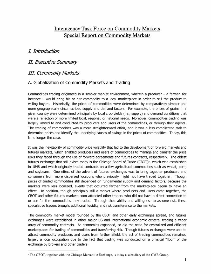
B. Macroeconomic Variables 1. Global Economic Activity Rapid economic growth has been the key driver of global demand for commodities in recent years. As shown in Figure 1, world real GDP growth averaged close to 5 percent per year from 2004 through 2007, marking the strongest performance in two decades. Economic growth was been particularly robust in developing economies, where real GDP rose at an average annual rate of more than 7 percent over the same time period. As a result of this growth, the world economy is about 25 percent larger than it was just 5 years ago, and the emerging market economies of Asia, including China and India, are roughly 50 percent larger. Over the past few months, however, prospects for continued robust economic growth have dimmed considerably, and global economic growth in the near term is likely to be dramatically lower than earlier this year. As a consequence, global demand for commodities has decelerated dramatically. Figure 1 World GDP

4

In addition to the pace of world economic activity, demand for commodities has been further supported in recent years by the composition of growth across countries. As shown in Figure 2, China, India, and the Middle East use substantially more oil and steel to produce a dollar�s worth of real output than the United States. These economies have been among the fastest growing in the world; together they have accounted for about two-thirds of the rise in global use of oil and steel since 2004. Moreover, these economies� use of commodities is still relatively low on a per capita basis, as shown in Figure 3. Over the longer term, as these economies continue to develop and incomes rise, per capita commodity use is likely to increase further. Figure 2 Commodity Intensity

Figure 3 Per Capita Commodity Use

2. Exchange Rates The relationship between exchange rates and commodity prices is complex, and the causality can run in both directions. Typically, a depreciation of the dollar would be expected to lead to a rise in the

5

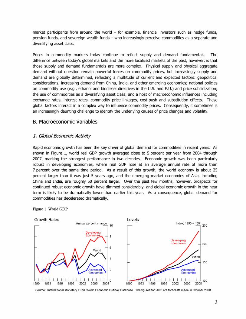
dollar price of commodities. As most commodities are priced in dollars, a lower exchange value of the dollar reduces the foreign-currency price and thus boosts demand. To clear the market, the dollar commodity price must then rise, assuming (reasonably) that supply is not perfectly elastic. Empirical studies do not reveal a clear, precisely estimated relationship between commodity prices and the exchange value of the dollar. Part of the difficulty in identifying such a relationship stems from the fact that many different factors can influence commodity prices and exchange rates in different ways at different times. However, the evidence that is available suggests that commodity prices respond approximately proportionately to changes in the dollar when all other economic factors are held constant. In other words, a 10 percent depreciation of the nominal, trade-weighted, multilateral exchange value of the dollar is associated with a 10 percent rise in the dollar price of commodities when other factors are held constant. That finding suggests that the depreciation of the dollar from early 2002 to mid 2008 contributed to the rise of dollar commodity prices, but explains only a portion of the overall run-up. This point is also evident in Figure 4, which graphs oil prices and an index of non-fuel commodity prices in several currencies. Clearly, commodity prices, particularly oil prices, rose markedly through the middle of 2008 regardless of the currency of denomination. Since then, however, the dollar has appreciated and commodity prices have plummeted, but, again, only a fraction of the fall in the dollar price of commodities appears to stem from exchange rate movements. Figure 4 Commodity Prices in Several Currencies

In the case of oil, an additional linkage between exchange rates and oil prices may arise through the production decisions of key oil exporters. Oil exporters suffer a decline in the purchasing power of their revenues when the dollar depreciates. To defend their international purchasing power, these producers could, in principle, seek an offsetting increase in the dollar price of oil by curtailing supply. Shocks specific to commodity markets can also feed back into exchange rates. During the past few years, the nominal value of U.S. oil imports has soared along with oil prices, resulting in a significantly wider trade deficit than would have otherwise occurred. This widening may have exacerbated concerns about the sustainability of the current account deficit, thereby putting downward pressure on the dollar.

6

3. Interest Rates The relationship between interest rates and commodity prices can vary, as it depends on the interactions of many economic variables. As noted below, a decline in interest rates by itself might be expected to raise commodity prices to some extent, suggesting a negative correlation between these two variables. But if the decline in interest rates is in reaction to a downturn in economic activity, commodity prices may very well fall in response to that weaker demand, resulting in a positive correlation. One mechanism by which declines in interest rates could push up commodity prices is through a reduction in the costs associated with storing commodities. An implication of this hypothesis is that inventories of commodities should tend to rise when interest rates decline. Such increases, however, are not evident in the available data. 4. Prices and Expectations Commodities are traded in global markets that are generally deep and liquid. Commodity prices adjust through markets to equilibrate the amounts supplied and demanded. For some commodities, such as oil, corn and wheat, the quantity consumed changes only modestly in response to price movements; that is, demand is relatively inelastic in the short run. For other commodities the quantity consumed changes more dramatically in response to price movements; demand is relatively elastic. The elasticity of demand for a commodity or good reflects the importance of the commodity to consumers and the availability of substitutes. For example, there are few substitutes for oil, especially for use in transportation. Demand for most goods is more elastic in the long run, as persistent high prices lead consumers and firms to make permanent changes to reduce the quantity used. The change in the quantity of a commodity produced in response to changes in price defines the elasticity of supply. Many agricultural commodities are thought to have inelastic short run supply because of growing seasons and lags in adjustment, but much more elastic long run supply. Oil producers often have more scope than consumers to respond to price changes, although at present the ability to adjust output in the near-term appears to be limited. The elasticity of demand and supply will determine the degree to which changes in supply and demand result in changes in quantity and changes in price. Goods with inelastic short run (one to two years) supply and demand � like many commodities - are likely to experience large swings in price in response to changes in supply or demand. Many of the commodities discussed in this report � most notably oil � are exhaustible resources. Oil is an exhaustible resource with a natural, inexpensive storage solution. This leads owners of oil reserves to base output decisions on both current prices and expectations of future prices. In particular, the pace at which they extract oil will depend on expectations about future prices relative to the risk-adjusted rate of return on other investments. Producers will supply less oil today and instead keep it in the ground if its price is expected to rise in the future by more than the expected return on other investments. Producers will pump more oil when the price is expected to fall (or rise at a rate slower than the return on other investments). Because today�s oil prices reflect expectations about future supply and demand, they can move considerably in response to events or changes in market

7

perceptions about future supplies, even if the events have little apparent connection with the supply or demand for oil today.

C. Instruments and Investors in Commodity Markets For much of the history of derivatives markets in the U.S., trading was primarily limited to hedgers and individual speculators trading on futures exchanges. This situation began to change in the 1980s when financial engineers developed the swap contract, giving hedgers and speculators an alternative to the exchange-traded futures contract to manage or acquire commodity price risks. More recently, commodity index funds, and exchange-traded funds and notes have been created that also allow portfolio managers and individuals to efficiently gain price exposures to individual commodities and commodity indexes through an alternative means to the futures markets. 1. Over-the-Counter Swap Contracts The development of the swap contract began in 1981 when the World Bank and IBM entered into what became known as a currency swap. The swap essentially involved a loan of Swiss francs by IBM to the World Bank and the loaning of U.S. dollars by the World Bank to IBM. The motivation for the transaction was the ability of each party to borrow the funds more cheaply than the counterparty, thereby reducing overall funding costs for both parties. This structure of swapping cash flows ultimately served as the template for swaps on any number of financial assets and commodities. Although currency swaps initially served a lending function, the development of swaps that exchange a fixed rate for a floating rate were found to serve as an effective hedging vehicle in much the same was that futures contracts do. For example, a futures contract is essentially a contract for the buyer of the contract to pay a fixed price in return for receiving delivery of a commodity that will have an uncertain or floating value. The advantage that swaps contracts offered, however, was the flexibility with which counterparties could tailor the terms of the contract to meet their hedging needs. For example, an airline wanting to hedge future jet fuel purchases cannot directly do so with a futures contract since none exists. Such hedging would have to be done as a cross hedge using crude oil, gasoline or heating oil futures. The swap market offers the airline the alternative of entering in to a swap contract that would directly reference a cash price for jet fuel. In addition to permitting the tailoring of contract terms to match such specifications as commodity, grades, and delivery timing and locations, swaps also allow counterparties to execute large positions that might overwhelm liquidity in a market. Thus, a hedger or speculator seeking a commodity exposure can obtain price certainty when negotiating a contract. The party offering the swap, typically a swap dealer, would take on any price risks associated with managing the risk of the commodity exposure. In the early development of swaps markets, investment banks often served in a brokering capacity to bring together parties with opposite hedging needs. The currency swap between the World Bank and IBM was brokered by Solomon Brothers. While brokering swaps eliminates market and credit risk to the broker, the process of matching and negotiating swaps between counterparties with opposite hedging needs could be difficult. As a result, swaps brokers, who took on no market risk, evolved into swaps dealers, who took the contract onto their books. This, of course, exposed the dealer to the risks

8

associated with commodity price movements. However, since a swap dealer is willing to enter into a swap contract on either side of a market, at times they will enter into swaps that create offsetting exposures. Since it is unlikely that a dealer at all times could completely offset the market risks associated with its swap business, dealers will often enter the futures markets to offset the residual market risk. As a result of the growth of the swaps market and the dealers who support the market, we have seen an associated growth in the futures markets related to the commodities for which swaps are offered.

2. Exchange-Traded Products Commodity exchange-traded products, or ETPs, refer to exchange-traded investment vehicles that offer investors exposure to a range of individual commodities, derivatives on commodities, and commodity indexes. The main types of commodity ETPs are commodity trust shares and commodity-linked notes (ETNs). Commodity trusts hold physical commodities or derivatives on these commodities and the investments are held in trust for the benefit of shareholders. Shares in the trust can be bought and sold throughout the day like stocks on a securities exchange through a broker-dealer. The shares of the trust should trade at approximately the same price as the net asset value of its underlying assets over the course of the trading day. If a commodity trust were liquidated, investors would receive their share of the underlying trust assets. Originally marketed as a tool for investors to participate in tradable portfolio or basket products, shares in commodity trusts are held today in large amounts by institutional investors, including mutual funds, and other investors as part of sophisticated trading and hedging strategies. Investors may short sell commodity trusts in the same manner that shares of stock can be sold short. Although commodity trust shares resemble exchanged-traded fund (ETF) shares, there is an important legal distinction between the two. Commodity trust shares are registered by the SEC under the Securities Act of 1933 whereas ETFs are also registered as investment companies under the Investments Company Act of 1940 (�1940 Act�). As such, commodity trusts are not subject to the same regulation of operations that applies to registered investment companies under the 1940 Act. Commodity-linked exchange-traded notes (ETNs) are senior, unsecured, unsubordinated debt securities issued by an underwriting bank or other large issuer. The issuer of the commodity ETN promises to pay a specified return, often linked to the performance of an underlying commodity derivative or commodity index minus an expense ratio. ETNs share both equity and debt attributes. ETNs have a maturity date and are backed only by the credit of the issuer. If investors hold the ETN to maturity, they will receive a cash payment that is linked to the performance beginning on the trade date and ending at maturity. In the event of default, ETN investors would receive their funds only if there was money left over after the secured creditors were paid. ETNs may be bought and held or else sold before maturity by trading them on the exchange. The additional risk of an ETN versus a commodity trust lies in the credit risk of the issuer. The issuer may suffer a decline in its credit rating or the underwriting bank could go bankrupt, adversely affecting the value of the ETN. ETNs do not accrue or pay out interest, unlike traditional debt securities. Investors may short sell ETNs. ETNs are regulated by the SEC under the 1933 Securities Act.

9

Investors can also gain exposure to commodities through three other types of investments: commodity-linked medium term notes, commodity index-linked mutual funds, and commodity index assets under management attributable to institutional investors. Commodity-linked medium term notes (MTNs) are structured products that involve a pre-packaged investment strategy that is based on derivatives, a basket of securities, commodities, or some other underlying security. Commodity-linked MTNs are primarily structures linked to commodity indices and may be associated with agriculture, metals, or other commodities. Commodity index assets under management are based on baskets of commodity futures which replicate the buying of a forward position that is continuously rolled forward in time. The positions are long only and there is no physical ownership of the underlying inventory. A 2008 study conducted by researchers at Barclays4 estimates a total value of $225 billion invested across the various commodity products. They give a breakdown as follows: $46 billion attributed to ETPs, $40 billion for MTNs, $17 billion for index-linked mutual funds, and $122 billion in index assets under management. 3. Commodity Index Funds A more recent development in the derivative market has been the development of commodity index funds. While investors have for years been able to invest in commodity pools, which pooled investors� funds to trade commodities much like mutual funds do for investors in stocks and bonds, commodity index funds offer investors the opportunity to gain a passive exposure to a specified index of commodities. That is, while a pool operator seeks to profit by following a trading strategy that may buy or sell a variety of commodities, the operator of commodity index fund seeks to match a pre-specified index through the acquisition of long futures positions.5 The major attraction of these funds are that they are believed to give investors a commodity exposure that is largely independent or even negatively correlated with the returns on stocks and bonds, and they eliminate margin calls against customers by entering into only long positions and trading on an unleveraged basis. Thus, a pension fund or other portfolio manager can theoretically smooth out the returns of a portfolio by including a commodity index position in the portfolio. Smaller retail investors have also embraced commodity index funds as a cost effective way of investing in a diverse basket of commodities. Moreover, because the funds only enter into long positions and have collected the full price for the commodity positions that they enter into, the risk of margin calls, which would be associated with a futures position, is eliminated.

4. CFTC Special Calls Report To better understand how swaps dealers and index traders use the futures markets to manage their risks, in June 2008, the CFTC issued a special call to swaps dealers and commodity index traders, which included 43 request letters issued to 32 entities and their sub-entities. These entities include

4 Cooper, S., K. Norrish, and A. Sen, July/August 2008, �Piercing the Fog: Facts and Fallacies about Commodity Investment Flows,� Futures Industry. 5 Theoretically an index could include short market positions, however, to date commodity index funds have primarily limited themselves to long positions. Moreover, the funds limit leverage to their customers by limiting the notional value of the fund to the amount of funds collected from its customers.

10

swap dealers engaged in commodity index business, other large swap dealers, and commodity index funds. The special call required all entities to provide data relating to their total activity in the futures and OTC markets, and to categorize the activities of their customers for month-end dates beginning December 31, 2007 through June 30, 2008, and continuing thereafter. On September 11, 2008, the CFTC issued a staff report that summarized the preliminary analysis of data collected through the special calls. The preliminary survey results represent the best data currently available to the staff and the results present the best available snapshot of swap dealers and commodity index traders for the relevant time period.6 In analyzing the total OTC and on-exchange positions for index trading, the report focuses on three quarterly snapshots � December 31, 2007, March 31, 2008, and June 30, 2008 - and has thus far revealed the following: Firstly, the estimated aggregate net amount of all commodity index trading (combined OTC and on-exchange activity) on June 30, 2008 was $200 billion, of which $161 billion was tied to commodities traded on U.S. markets regulated by the CFTC. Of the $161 billion combined total, a significant amount of the OTC portion of that total likely is never brought to the U.S. futures markets. For comparison purposes, the total notional value on June 30, 2008 of all futures and options open contracts for the 33 U.S. exchange-traded markets that are included in major commodity indexes was $945 billion � the $161 billion net notional index value was approximately 17 percent of this total. Secondly, the staff report also presented index trading data for some individual commodities. The total notional value of futures and options open contracts on June 30, 2008 for NYMEX crude oil was $405 billion � the $51 billion net notional index value was approximately 13 percent of this total. The total notional value of futures and options open contracts on June 30, 2008 for CBOT wheat was $19 billion � the $9 billion net notional index value was approximately 47 percent of this total. The total notional value of futures and options open contracts on June 30, 2008 for CBOT corn was $74 billion - the $13 billion net notional index value was approximately 18 percent of this total. The total notional value of futures and options open contracts on June 30, 2008 for ICE-Futures US cotton was $13 billion � the $3 billion net notional index value was approximately 23 percent of this total. Finally, according to the report, of the total net notional value of funds invested in commodity indexes on June 30, 2008, approximately 24 percent was held by �Index Funds,� 42 percent by �Institutional Investors,� 9 percent by �Sovereign Wealth Funds,� and 25 percent by �Other� traders.

D. The Role of Commodity Futures Markets 1. Futures Contract Design

6 As a result of the survey limitations, there may be a margin of error in the precision of the data, which will improve as the staff continues to work with the relevant firms and to further review and refine the data. As entities continue to provide monthly data to the Commission in response to their ongoing obligation to comply with the special call, Commission staff will continue to examine the data, refine the specific requests, and further develop the analysis.

11

A futures contract is an agreement between two parties to buy and sell a given amount of a commodity at an agreed upon date in the future, at an agreed upon price and at a given location. For example, the Chicago Board of Trade (CBOT) December 2008 corn contract is an agreement to deliver 5,000 bushels of No. 2 yellow corn via a shipping certificate within the Chicago and Burns Harbor, Indiana shipping districts along the Illinois waterway during the first half of December 2008. Similar scenarios hold true for the CBOT�s soybean and wheat contracts. In this regard, the CBOT November 2008 soybean contract calls for the transfer of 5,000 bushels of No. 2 yellow soybeans via a shipping certificate at the same delivery points as for corn during the first half of the contract month. The CBOT wheat contract calls for the delivery of 5,000 bushels of No. 2 soft red winter, No. 2 hard red winter, No. 2 dark northern spring, and No. 2 northern spring wheat using a shipping certificate at either the Chicago; Burns Harbor, Indiana; or Toledo, Ohio; shipping districts. In the case of crude oil, the New York Mercantile Exchange (NYMEX) West Texas Intermediate (WTI) December 2008 oil contract is an agreement to physically deliver 1,000 barrels (42,000 gallons) of oil at Cushing, Oklahoma during the contract month. For all futures contracts, the buyer (or long trader) and the seller (or short trader) agree to a price when they enter into the contract. Unless offset, these contracts require their counterparties to deliver or to take physical delivery of a commodity.7 A party whose contract remains open at its expiration date is obligated to make or take delivery as promised. Futures contracts are standardized so as to facilitate trading between buyers and sellers. The characteristics of a contract specify common commodity grades and quantities that are typically seen in the cash market transactions. The specificity of deliverable grades varies across futures contracts. In general, futures contracts specify deliverable grades that are commonly traded in the cash market. However, the number of deliverable graded varies from contract to contract. This feature is particularly true for agricultural futures contracts. In this regard, weather and disease play important roles in crop development. Adverse growing conditions may reduce the availability of the par grade, thus making delivery difficult. In contrast, favorable conditions may produce and overabundance of higher grades. Crop futures assume average growing conditions. Thus, the futures contracts specify average commodity grades, which reflect crop quality that is realized by most farmers in most crop years. In order to account for the effect of adverse or favorable weather conditions on crop quality, crop futures contracts allow the delivery of additional grades at a premium or discount. For example, lower grades of corn, such as No. 3 yellow corn, are deliverable on the CBOT corn contract at a discount of 1.5 cents per bushel. Dominant futures contracts within a specific group typically are listed on a single exchange. In this regard, livestock products are listed on the Chicago Mercantile Exchange (CME), energy contracts are listed on the NYMEX, and row crop futures are listed on the CBOT. Exceptions do exist, particularly if a similar contract listed by another exchange specifies a different variety or grade of the same underlying commodity. For example, while the CBOT offers the dominant wheat contract, the Minneapolis Grain Exchange and Kansas City Board of Trade both offer their own wheat contracts. The MGE contract specifies No. 2 northern spring wheat, while the KCBT contract calls for the delivery of No. 2 hard red winter wheat. Contract terms and conditions, such as delivery and storage procedures, reflect standard industry practices. While a given futures contract�s terms and conditions mirror common characteristics associated with cash market transactions, futures contracts� terms and conditions generally are not

7 Not all futures contracts require physical delivery.

12

standard across contracts. For example, delivery requirements can vary greatly. The NYMEX crude oil contract requires that the seller physically transfer the crude oil to the buyer in Cushing during the contract month. In contrast, the CBOT corn, soybeans, and wheat futures contracts are physically settled contracts which deliver the commodity to the buyer in the form of a shipping certificate. The delivery instrument (shipping certificate) gives the buyer the right but not the obligation to demand load-out of the commodity whenever desired. The regular firm approved for delivery who issued the shipping certificated loads out the commodity within the timeline mandated by the exchange rules. The shipping certificate represents a claim to a commodity without binding the owner to a specific stock in a specific location. Shipping certificates offer the owner flexibility since there are no timelines in which one must convert the certificate into the physical commodity. During the time an owner holds the certificate he incurs opportunity cost and a set storage cost that must be paid to the regular firm. Additional shipping certificates (SC) features include the holder�s ability to sell the certificate in the cash market, sell it back to the issuing firm, or redeliver the certificate against an expiring short position. 2. Risk Management and Price Discovery Because futures contracts are standardized futures markets are ideal for aggregating a multiplicity of opinions regarding the expected price of a commodity at different points in time in the future. It is often easier for a common view on an expected price to emerge at a futures exchange than among dispersed producers and consumers of a physical (cash) commodity. For that reason, futures markets are an important source of price information - prices are often said to be �discovered� in futures markets and then communicated to participants in certain cash markets. The price discovery function of futures markets is extremely valuable in terms of planning business activities and for allocating commodity price risk. Futures contracts are instruments primarily designed to manage risk - they are identical in all aspects except for the contracted price; they trade on exchanges; and clear through designated clearinghouses. Exchange trading may occur either electronically or on the floor through open outcry; many times electronic and floor trading are conducted simultaneously. For crude oil and each of the row crops, the primary futures contract is physically delivered. Energy traders tend to have a greater array of choices with respect to contracts that are usable for risk management purposes. Besides the dominant physically-delivered contracts, energy traders can take advantage of cash-settled futures, mini-sized contracts, and basis contracts. In contrast, nearly all crop futures are physically delivery. The MGE does offer for trading cash settled corn, soybeans, and wheat contracts based on national index prices. However, none of these MGE contracts achieved significant trading volume since their introduction in early- and mid-2000. Due to their standardization, futures contracts are not so well-suited to allocate the physical commodity. For example, to mainly serve an allocation role, crude oil futures contracts in particular would feature multiple delivery locations. In fact, the figure below shows, only a small number of oil futures contracts result in physical delivery. Similarly, even though some futures contracts, such as those for corn and soybeans, specify a multiplicity of delivery points, the multiple delivery points are intended to facilitate delivery on the contract for the purpose of attaining better convergence between cash and futures prices rather than facilitating the use of the contracts as merchandizing vehicles.

13

3. Hedging and Speculation The distinction between hedging and speculation in futures markets is less clear than it may appear. Traditionally, those with a commercial interest in or an exposure to a physical commodity have been called hedgers, while those without a physical position to offset have been called speculators. In practice, however, hedgers may be �taking a view� on the price of a commodity, and even those who are not participating in the futures market despite having an exposure to the commodity could be considered speculating. Traditional speculators enter into futures contracts with the intention of reversing their positions before they would be required to deliver (short positions) or to accept physical delivery (long positions) of a commodity. As such, speculators serve important market functions � immediacy of execution, liquidity, and information aggregation. Traditional speculators could further be differentiated depending on the time horizons at which they operate. Speculators, known as scalpers or market makers, operate at the shortest time horizon � sometimes trading within a single second. These traders typically do not trade with a view as to where prices are going. Instead, they provide immediacy of execution to a trade. That is, they �make markets� by standing ready to buy or sell at a moment�s notice. These market makers will usually offset their positions soon after entering into them. The goal of a market maker is to buy contracts at a slightly lower price than the current market price and sell them at a slightly higher price, perhaps at only a fraction of a cent profit on each contract. By trading hundreds or even thousands of contacts a day, skilled market makers can earn a profit. The benefit provided by the market maker is the speed, or immediacy, at which a trader attempting to establish or offset a position in the market can do so. Absent a market maker, a market participant would have to wait until the arrival of another party with an opposite trading interest. Other types of speculators take longer-term positions based on their view of where prices may be headed. Speculators known as �day traders� establish positions based on their views of where prices might be moving in the next minutes or hours, while �trend followers� take positions based on price expectations over a period of days, weeks or months. Through their efforts to gather information on underlying commodities, the activity of these traders serves to bring information to the markets and aid in price discovery. These speculators are also important to the market in that they often supply overall liquidity to hedgers in futures market. While hedging and speculation are often considered opposite activities and are generally identified with commercial and non-commercial traders, in practice both commercial and non-commercial traders can bring about the price discovery in futures markets. In essence, futures prices are a reflection of the opinions of all those entering the market. Moreover, the actions of those who can, but choose not to enter the futures market are also quite important for price discovery. For example, a commercial trader holding physical inventory, but choosing not to hedge it in the futures market (by taking a short position) will not only withhold a downward pressure on the price, but may also send a signal that prices are expected to rise in the future. It is important to keep in mind that futures and option trading should be viewed in the context of an overarching risk management strategy. Futures trading may be only one means of hedging price risk. Market participants may be involved concurrently in OTC transactions, trades on exempt commercial

14

markets, and transaction in foreign markets. For example, crude oil traders can hedge cash market positions using a combination of futures, swaps, bilateral forward contracts, and cleared broker and ECM transactions. Grain traders can use a combination of forward and hedge-to-arrive contracts as well as exchange-traded futures and options, and agricultural swaps. Activities that occur in other markets and other instruments can also impact futures markets. There are three potential activities that might impact futures trading on U.S. exchanges: (i) the trading of over-the-counter (OTC) derivatives contracts ; (ii) the trading on exempt commercial markets; and (iii) the trading on foreign boards of trade.

4. Publicly Available Data on Futures Markets To provide the public with information on the activity of traders in the futures and options markets, the CFTC publishes a weekly Commitments of Traders (COT) report. The report is released every Friday at 3:30 p.m. Eastern time and contains a summary of trader�s positions as of the close of business on the previous Tuesday for each market in which 20 or more traders hold positions equal to or above the large trader reporting levels established by the CFTC.8 The summary of market activity contained in the weekly COT reports is available in a variety of formats�i.e., long and short format, as well as in futures-only and futures-and-options-combined format�and are available for no charge on the CFTC�s website. The long and short format reports show open interest separately by reportable and non-reportable positions. For reportable positions, additional data is provided for commercial and non-commercial holdings, spreading, changes from the previous report, percents of open interest by category, and numbers of traders. The long report also groups the data by crop year, where appropriate, and shows the concentration of position held by the largest four and eight traders. The CFTC, beginning in 2007, also publishes a Supplemental report for selected agricultural markets showing all the information in the short format report plus the positions of traders classified as Index Traders.9 The information regarding the reportable positions of traders contained in the COT reports is drawn from the reports the CFTC receives daily from clearing members, futures commission merchants, and foreign brokers. Those reports show the futures and option positions of traders that hold positions above specific reporting levels set by CFTC regulations. If, at the daily market close, a reporting firm has a trader with a position at or above the CFTC�s reporting level in any single futures month or option expiration, it reports that trader�s entire position in all futures and options expiration months in that commodity, regardless of size. The aggregate of all traders� positions reported to the CFTC usually represents 70 to 90 percent of the total open interest in any given market. From time to time, the CFTC will raise or lower the reporting levels in specific markets to strike a balance between collecting

8 Reporting levels can be found in section 15.03(b), 17 CFR15.03(b), of the CFTC�s regulations, and can be accessed from the CFTC�s website, www.cftc.gov 9 For more information on the CFTC�s Supplemental report see, �Commodity Futures Trading Commission: Commission Actions in Response to the �Comprehensive Review of the Commitments of Traders Reporting Program� (June 21, 2006),� available at the CFTC�s website, www.cftc.gov.

15

sufficient information to oversee the markets and minimizing the reporting burden on the futures industry. When an individual reportable trader is identified to the CFTC, the trader is classified either as �commercial� or �non-commercial.� All of a trader�s reported futures positions in a commodity are classified as commercial if the trader uses futures contracts in that particular commodity for hedging as defined in CFTC Regulation 1.3(z), 17 CFR 1.3(z). Generally this definition reflects a matching of a futures position with a commercial market risk and does not consider the motivation for entering into a hedge. A trading entity generally gets classified as a �commercial� trader by filing a statement with the CFTC, on CFTC Form 40: Statement of Reporting Trader, that it is commercially ��engaged in business activities hedged by the use of the futures or option markets.� To ensure that traders are classified with accuracy and consistency, CFTC staff may exercise judgment in re-classifying a trader if it has additional information about the trader�s use of the markets. A trader may be classified as a commercial trader in some commodities and as a non-commercial trader in other commodities. A single trading entity cannot be classified as both a commercial and non-commercial trader in the same commodity. Nonetheless, a multi-functional organization that has more than one trading entity may have each trading entity classified separately in a commodity. For example, a financial organization trading financial futures may have a banking entity whose positions are classified as commercial and have a separate money-management entity whose position are classified as non-commercial. In classifying traders as commercial or non-commercial rather than hedgers and non-hedgers, the CFTC recognizes that the ultimate motivations for trading futures by commercial and non-commercial traders cannot be observed. That is, while a commercial trader may be matching a futures position against a cash market price risk, it is not known whether such a trader is doing so on a routine basis in order to minimize ongoing price risks or doing so selectively based on specific market expectations. Thus, some of the trading information captured by the commercial trading category may reflect activity that could be characterized more as speculative rather than hedging.

IV. Select Commodity Markets: Fundamentals and Markets

A. Crude Oil

1. Background The recent, rapid crude oil price rise and fall represent an extension of oil market developments originating in the 1990s. At around that time, relatively high inventories and ample surplus production capacity served to limit oil price fluctuations. When spot market prices moved up or down, futures contracts requiring delivery in distant months generally traded close to $20 per barrel, consistent with a market expectation that producers would ensure that spot prices would eventually return to that level. However, as leading Organization of Petroleum Exporting Countries (OPEC) members shifted towards a tight inventory policy and global oil demand recovered from the slowing effect of Asia�s financial crisis, the global market balance tightened and inventories declined sharply at the beginning of the present decade. Oil prices rose to $30 per barrel in what might be seen as the first leg of the upward trend. By 2003, inventories were drawn down sufficiently such that subsequent increases in global demand stretched oil production to levels near capacity. The large, unexpected jump in world oil consumption

16

growth in 2004, fostered by strong growth in economic activity in Asia, reduced excess production capacity significantly. Into the first half of 2008, despite high prices, world oil consumption growth remained strong, overall non-OPEC production growth continued to slow, and OPEC oil production could not fill the gap. Geopolitical risks created considerable uncertainty about future supplies. Crude oil price declines since mid-July reflect an increasingly clear slowdown in oil consumption growth, higher recent Saudi Arabian oil production, and prospects of higher non-OPEC supplies through 2009. The resulting lower demand for OPEC oil, combined with planned increases in OPEC production capacity, now suggests OPEC surplus crude production capacity could increase to about 3 million barrels per day next year, providing the market with a cushion against supply disappointments and supporting lower oil prices than expected previously. Turmoil in U. S. financial markets point to lower global economic activity and weaker world oil consumption growth and has reinforced the sentiment of a loosening in the global oil balance. EIA�s November release of its Short Term Energy Outlook, reflected a considerable reduction in expected world oil prices for the second half of 2008, with moderate price growth through the first half of 2009. This forecast reflects the clear global downturn and its effects on demand for energy. EIA�s November Outlook recognizes OPEC�s intention to cut crude oil production starting November 1, in response to a perceived supply surplus in the market caused by slowing oil consumption growth and higher non-OPEC supply growth. The result is that the OPEC production cut may limit, but not reverse the recent sharp fall in oil prices.

2. Demand

a. Global Economic Activity

The key driver of oil demand has been robust global economic growth, particularly in emerging market economies. As shown in Figure 1, world GDP growth (with countries weighted by oil consumption shares) has averaged close to 5 percent per year since 2004, marking the strongest performance in two decades.

Figure here. In addition to the pace of world economic activity, oil demand has been further supported by the composition of growth across countries. As shown in Figure 2, China, India, and the Middle East use substantially more oil to produce a dollar�s worth of real output than the United States.

Figure here. These economies are among the fastest growing in the world; together they have accounted for nearly two-thirds of the rise in world oil consumption since 2004. Moreover, these economies still consume relatively little oil on a per capita basis. Over the longer term, as these economies continue to develop and incomes rise, per capita energy use is likely to increase further.

b. Increasing Consumption

17

The historical rise in global economic activity has been accompanied by corresponding growth in world oil consumption. Since 2003, world oil consumption growth has averaged 1.4 percent per year. The recent global economic slowdown, however, is expected to result in virtually no growth for 2008, reaching only 85.9 million barrels a day. Non-OECD countries, especially China, Brazil, India, and the Middle East, represent the vast majority of currently expected growth (Figures 3 and 4).

Figure [ ] Annual Growth in World Oil Consumption

2003 2004 2005 2006 2007 2008

Ch

an

ge

fro

m P

rio

r Y

ear

(Mill

ion

Ba

rre

ls p

er

Day

C hina U.S . Other

1.6

2.7

1.41.1

0.9

T otal W orld Oil C ons umption Growth

0.7

Source: Energy Information Administration, Short-Term Energy Outlook September 2008

(est.)

(Million Barrels per Day)

18

Due both to higher prices in the first part of the year and and general economic weakness in the last part, world oil consumption is projected to remain effectively flat�growth of less than 0.1 percent in 2008, down from 0.9 percent growth in 2007. Higher oil prices have clearly led to a decline in OECD oil consumption. During the first half of 2008, total OECD oil consumption fell by 1,095,000 bbl/d (2.2 percent) compared to year-prior levels. In the U.S. alone, oil consumption fell by 930,000 bbl/d (4.5 percent). As the largest oil consumer in the world, this dramatic reduction in U.S. oil consumption is a crucial development in oil market fundaments that has led to falling prices in the past three months. However, non-OECD oil consumption growth in 2008 appears to have offset all of the decline in the OECD and seems less affected by higher world oil prices, because consumers in many of these countries are insulated from world market prices by domestic subsidies. Much of the non-OECD consumption is driven by overall economic activity, rather than discretionary use, so price effect upon oil consumption is mostly outweighed by the larger impact of economic growth. Later in 2008, the global economic slowdown may have reduced some of this consumption.

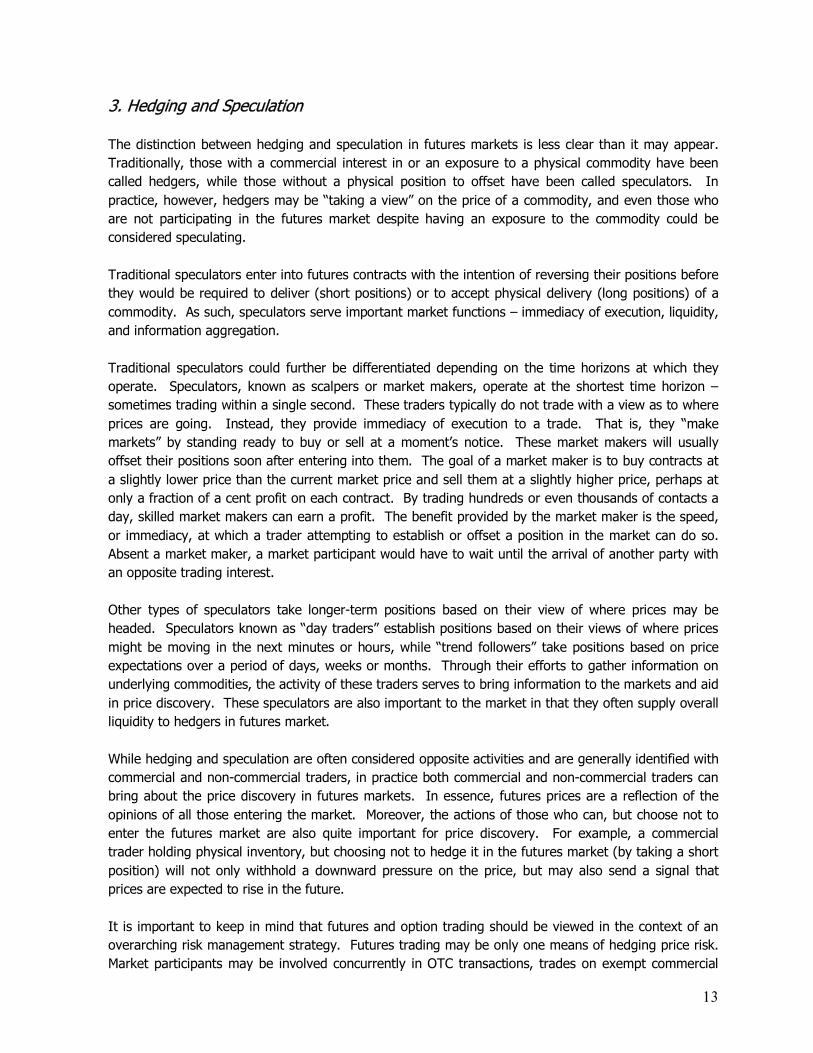
c. Price Controls and Subsidies

Many emerging market and developing economies use subsidies and other administrative measures to control domestic fuel prices. These administered prices are generally set below global market prices and, therefore, artificially push up the demand for oil. Indeed, a large portion of the increase in global oil consumption this year is expected to be in countries where fuel prices are subsidized and demand is not fully responsive to price signals. Price controls and subsidies interfere with the economic link between market prices and consumption.

Figure [ ] Oil Consumption Growth by Country from 2003 to 2008

T otal Oil C ons umption G rowth, 2003-2008 (Million bbl/d)

0.17

0.19

0.20

0.26

0.27

0.36

0.46

0.46

0.71

2.44

Argentina

Mex ico

Iraq

R us s ia

V enezuela

Iran

India

B razil

S audi Arabia

C hina

0.420.86

0.28 0.48 0.38 0.44

1.15

1.88

1.13 0.650.49 0.23

2003 2004 2005 2006 2007 2008

C hina

R es t of World

Source: Energy Information Administration, Short Term Energy Outlook September 2008

World Oil Consumption Growth (Millions of Barrels per Day)

Oil Consumption Growth (Millions of Barrels per Day)

19

3. Supply

a. Stagnant Production

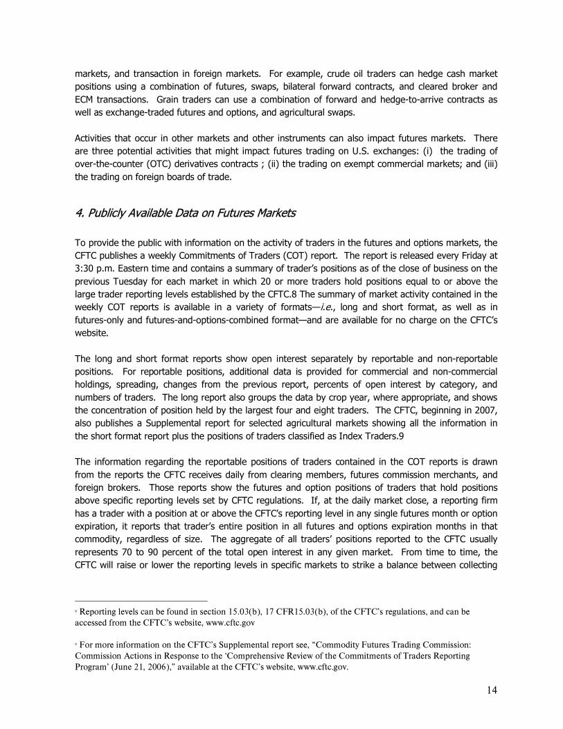
Global demand, while still growing in early 2008, appears to be falling in late 2008, largely due to global economic conditions. Overall non-OPEC production growth slowed throughout the year. In the past three years, non-OPEC production growth has been well below levels seen just four years ago. World oil consumption growth has simply continued to outpace non-OPEC production growth in every year since 2003 (Figure 5).

During the first half of 2008, world oil consumption increased by about 300,000 bbl/d from prior-year levels, while non-OPEC supply actually declined by about 300,000 bbl/d. This imbalance increased reliance on OPEC production and/or inventories to fill the gap. Over the last several years, OPEC has not kept up with this need for its oil: between 2003 and 2007, OPEC oil production (crude and other liquids) grew by 3.5 million barrels per day, while the �call on OPEC� (defined as the difference between world consumption and non-OPEC production) increased by 4.8 million barrels per day. As a result, the world oil market balance tightened significantly. In the latter half of 2008, while non-OPEC production is also expected to decline by about 300,000 bbl/d from the same period in 2007, worldwide consumption is expected to decline by about 400,000 bbl/d, reducing the demand for OPEC supplies. In addition, supply has appeared to increase from Saudi Arabia and elsewhere, at least for a period of time. Some sizeable non-OPEC production, such as

Figure [ ] Increasing Reliance on OPEC Production

1.6

2.7

1.4

1.1

0.9

0.1

0.6

0.8

1.11.0 0.9

-0.2

0.2 0.3

-0.3 -0.3

0.0

0.6

2003 2004 2005 2006 2007 2008Q1 2008Q2 2008Q3 2008Q4

Ch

an

ge

fro

m P

rio

r Y

ear

(Mill

ion

Bar

rels

per

Da

y

W orld Oil C onsumptionG rowth

Non-OP E C P roductionG rowth

Source: Energy Information Administration, Short-Term Energy Outlook September 2008

20

in Brazil and Azerbaijan, has started to come online, leading to an improved perception regarding non-OPEC supply growth for the second half of 2008 in comparison to the first half of the year.

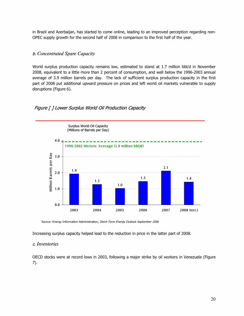
b. Concentrated Spare Capacity

World surplus production capacity remains low, estimated to stand at 1.7 million bbl/d in November 2008, equivalent to a little more than 2 percent of consumption, and well below the 1996-2003 annual average of 3.9 million barrels per day. The lack of sufficient surplus production capacity in the first part of 2008 put additional upward pressure on prices and left world oil markets vulnerable to supply disruptions (Figure 6).

Increasing surplus capacity helped lead to the reduction in price in the latter part of 2008.

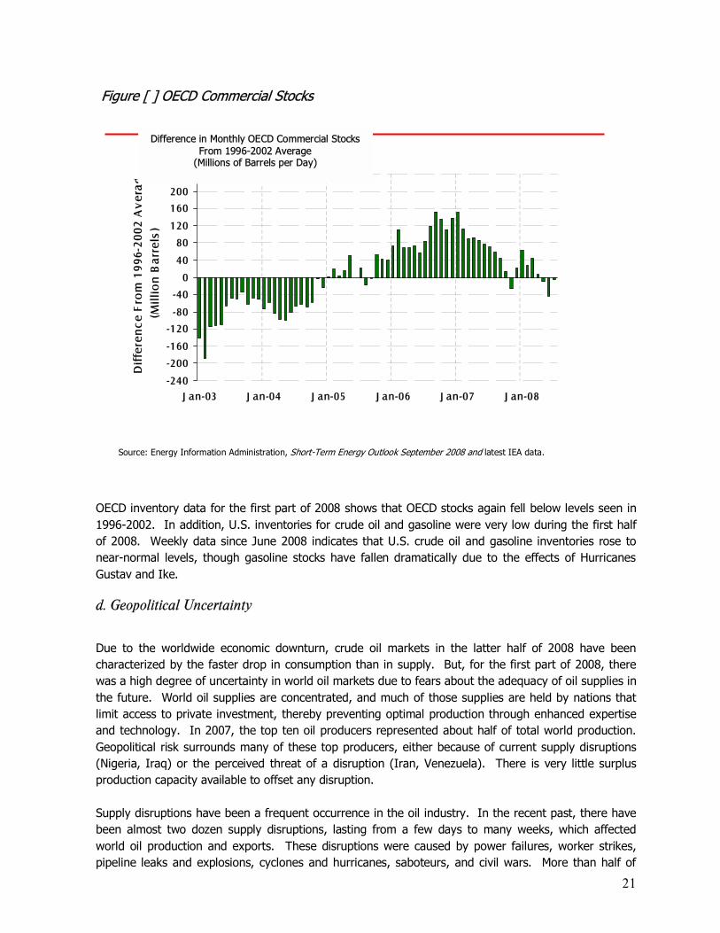
c. Inventories

OECD stocks were at record lows in 2003, following a major strike by oil workers in Venezuela (Figure 7).

Figure [ ] Lower Surplus World Oil Production Capacity

1.9

1.31.0

1.5

2.1

1.4

0.0

1.0

2.0

3.0

4.0

2003 2004 2005 2006 2007 2008 (es t.)

Mill

ion

Bar

rels

pe

r D

ay

1996-2002 His tor ic Average (3.9 million bbl/d)

Source: Energy Information Administration, Short-Term Energy Outlook September 2008

Surplus World Oil Capacity (Millions of Barrels per Day)

21

OECD inventory data for the first part of 2008 shows that OECD stocks again fell below levels seen in 1996-2002. In addition, U.S. inventories for crude oil and gasoline were very low during the first half of 2008. Weekly data since June 2008 indicates that U.S. crude oil and gasoline inventories rose to near-normal levels, though gasoline stocks have fallen dramatically due to the effects of Hurricanes Gustav and Ike.

d. Geopolitical Uncertainty

Due to the worldwide economic downturn, crude oil markets in the latter half of 2008 have been characterized by the faster drop in consumption than in supply. But, for the first part of 2008, there was a high degree of uncertainty in world oil markets due to fears about the adequacy of oil supplies in the future. World oil supplies are concentrated, and much of those supplies are held by nations that limit access to private investment, thereby preventing optimal production through enhanced expertise and technology. In 2007, the top ten oil producers represented about half of total world production. Geopolitical risk surrounds many of these top producers, either because of current supply disruptions (Nigeria, Iraq) or the perceived threat of a disruption (Iran, Venezuela). There is very little surplus production capacity available to offset any disruption. Supply disruptions have been a frequent occurrence in the oil industry. In the recent past, there have been almost two dozen supply disruptions, lasting from a few days to many weeks, which affected world oil production and exports. These disruptions were caused by power failures, worker strikes, pipeline leaks and explosions, cyclones and hurricanes, saboteurs, and civil wars. More than half of

Figure [ ] OECD Commercial Stocks

-240

-200

-160

-120

-80

-40

0

40

80

120

160

200

240

J an-03 J an-04 J an-05 J an-06 J an-07 J an-08

Dif

fere

nc

e F

rom

19

96-

20

02

Av

era

g

(Mil

lio

n B

arr

els

)

Source: Energy Information Administration, Short-Term Energy Outlook September 2008 and latest IEA data.

Difference in Monthly OECD Commercial Stocks From 1996-2002 Average

(Millions of Barrels per Day)

22

these resulted in oil production outages exceeding 100,000 barrels per day. The most significant of these to oil markets resulted from the ongoing strife in Iraq and Nigeria. These disruptions have varied in size over time, with Iraq losing more than 500,000 barrels per day of exports in March 2008 and Nigeria reaching more than 1.4 million barrels per day of shut-in production at one point in April 2008. Actual supply disruptions directly affect world oil markets due to a loss of physical barrels available to the market. Concern over the impact of potential supply disruptions is reinforced by the limited amount of spare production capacity available. As long as potential disruptions, either realized (as in Iraq and Nigeria) or perceived (as in concerns about the potential loss of supply from Iran), exceed the amount of additional production capacity that can be brought online quickly, geopolitical concerns will weigh heavily on oil markets.

4. Price-Inelastic Supply and Demand

The short-run demand for oil is relatively price inelastic, meaning the quantity demanded does not change much relative to price changes. Put another way, it takes a very large price increases to significantly reduce the quantity demanded. In the short run, the supply of oil is inelastic as well: the quantity supplied is not responsive to changes in market price, due to low spare capacity, the inability to bring new supplies online quickly, and relatively low inventories to draw down. If both supply and demand are not very responsive to prices, it takes large price increases to return markets to equilibrium if they get out of balance temporarily. As noted previously, world oil production has remained relatively flat in recent years, as global economic growth has kept demand strong. Consequently, oil prices have risen to keep world oil consumption in line with production. As oil demand is very insensitive to moves in oil prices in the near term, the rise in oil prices has been disproportionately large in order to offset the robust, income-driven rise in demand. An implication of these structural features of the oil market is that large and rapid movements in oil prices are not, by themselves, evidence that prices are behaving in a manner that is inconsistent with the fundamentals of demand and supply. Indeed, in such tight market conditions, relatively small changes in demand and supply should be expected to lead to large price swings. That said, there is a significant degree of uncertainty regarding the true state of market fundamentals at any point in time, due to the general lack of reliable and timely data.

5. Analysis of Crude Oil Futures Markets (update using additional data10

a. Broad Trends in the Participant Structure of Crude Oil Futures Markets

According to the publicly-available Commitments of Traders (COT) reports, activity in the West Texas Intermediate (WTI) light sweet crude oil contracts has grown steadily since 2000. In the last three and a half years alone, open interest across all available contract maturities (the

10 This section largely summarizes findings in an upcoming CFTC research paper analyzing changes in the level and composition of end-of-day open interest in the U.S. crude oil futures market. See Bόyόk�ahin, Haigh, Harris, Overdahl and Robe: �Market Growth and Trader Participation in Futures Markets,� CFTC � Office of the Chief Economist Working Paper, Fall 2008.

23

number of contracts open at the end of each day) in WTI futures and futures-equivalent (or �adjusted�) option contracts traded on the New York Mercantile Exchange (NYMEX) more than tripled from around 900,000 contracts in January 2004 to more than 2.75 million contracts in late August 2008. During the same period, the number of large traders also grew substantially � it almost doubled (from approximately 220 reporting traders in January 2004 to just under 400 in June 2008) before dropping back to 331 large option and futures traders as of late August 2008. These figures speak to the competitiveness and depth of the crude oil futures markets in the U.S. The COT reports also present the breakdown of the overall open interest between commercial and non-commercial traders grouped into long, short, and spread positions. While all types of positions have grown during the last three and a half years, the COT data suggests that it is the spread positions of non-commercial traders that have had the fastest growth rate. While overall open interest has tripled since 2004, non-commercial spread positions have increased six-fold. Notably, spread positions involve long positions in one month combined with short positions in another month so that spread traders are speculating on differences between futures prices in different months rather than the overall price level of crude oil. Since 2005, both the long and short positions of non-commercial traders have increased. Over that time period, the positions of non-commercial traders have been net long and have increased nominally; however, the proportion of those positions has been relatively constant as a share of the annual average open interest over the last few years.

b. Detailed Structure of Crude Oil Futures Markets

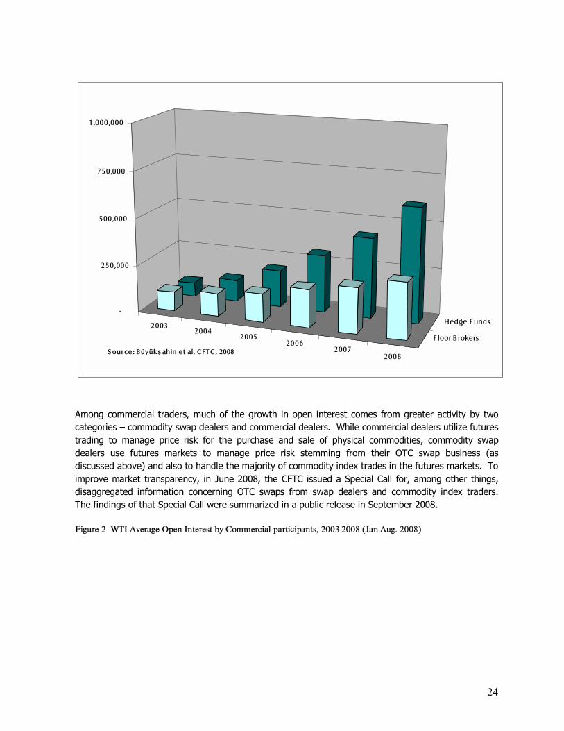
Whereas the publicly available data only identifies �commercial� and �non-commercial� categories of participants in the crude oil futures market, the COT report is built upon confidential CFTC data collected for market surveillance purposes which allows for a more precise categorization. For both analytical and presentational purposes, this confidential data was aggregated into broad sub-categories. Sub-categories for commercial participants include, among others, commercial producers, commercial manufacturers, commercial dealers, and swap dealers. Sub-categories for non-commercial participants include, among others, hedge funds and floor brokers and traders. These six commercial and non-commercial sub-categories account for approximately 80 percent of open interest in crude oil futures market. Figures 10 and 11 show that the increases in both commercial and non-commercial activity, as previously summarized in publicly available COT data, are broad-based. Among the non-commercial participants, both hedge funds and floor brokers and traders exhibit robust growth in open interest. Figure 1 WTI Average Open Interest by Non-Commerical participants, 2003-2008 (Jan-Aug. 2008)

24

20032004

20052006

20072008

F loor B rokers

Hedge F unds

-

250,000

500,000

750,000

1,000,000

S our ce: Büyük ş ahin et al, C FT C , 2008

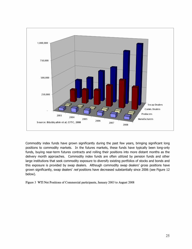
Among commercial traders, much of the growth in open interest comes from greater activity by two categories � commodity swap dealers and commercial dealers. While commercial dealers utilize futures trading to manage price risk for the purchase and sale of physical commodities, commodity swap dealers use futures markets to manage price risk stemming from their OTC swap business (as discussed above) and also to handle the majority of commodity index trades in the futures markets. To improve market transparency, in June 2008, the CFTC issued a Special Call for, among other things, disaggregated information concerning OTC swaps from swap dealers and commodity index traders. The findings of that Special Call were summarized in a public release in September 2008. Figure 2 WTI Average Open Interest by Commercial participants, 2003-2008 (Jan-Aug. 2008)

25

20032004

20052006

20072008

Manufacturers

Producers

Comm. Dealers

S w ap Dealers

-

250,000

500,000

750,000

1,000,000

S ource: Büyük ş ahin et al, C F T C , 2008

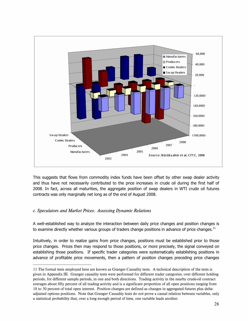
Commodity index funds have grown significantly during the past few years, bringing significant long positions to commodity markets. In the futures markets, these funds have typically been long-only funds, buying near-term futures contracts and rolling their positions into more distant months as the delivery month approaches. Commodity index funds are often utilized by pension funds and other large institutions that seek commodity exposure to diversify existing portfolios of stocks and bonds and this exposure is provided by swap dealers. Although commodity swap dealers� gross positions have grown significantly, swap dealers' net positions have decreased substantially since 2006 (see Figure 12 below). Figure 3 WTI Net Positions of Commercial participants, January 2003 to August 2008

26

20032004

20052006

20072008

Manufac turers

Producers

Comm. Dealers

S w ap Dealers (100,000)

(80,000)

(60,000)

(40,000)

(20,000)

-

20,000

40,000

60,000Manufacturers

Producers

Comm. Dealers

S w ap Dealers

S ource: Büyük ş ahin et al, C FT C , 2008

This suggests that flows from commodity index funds have been offset by other swap dealer activity and thus have not necessarily contributed to the price increases in crude oil during the first half of 2008. In fact, across all maturities, the aggregate position of swap dealers in WTI crude oil futures contracts was only marginally net long as of the end of August 2008.

c. Speculators and Market Prices: Assessing Dynamic Relations

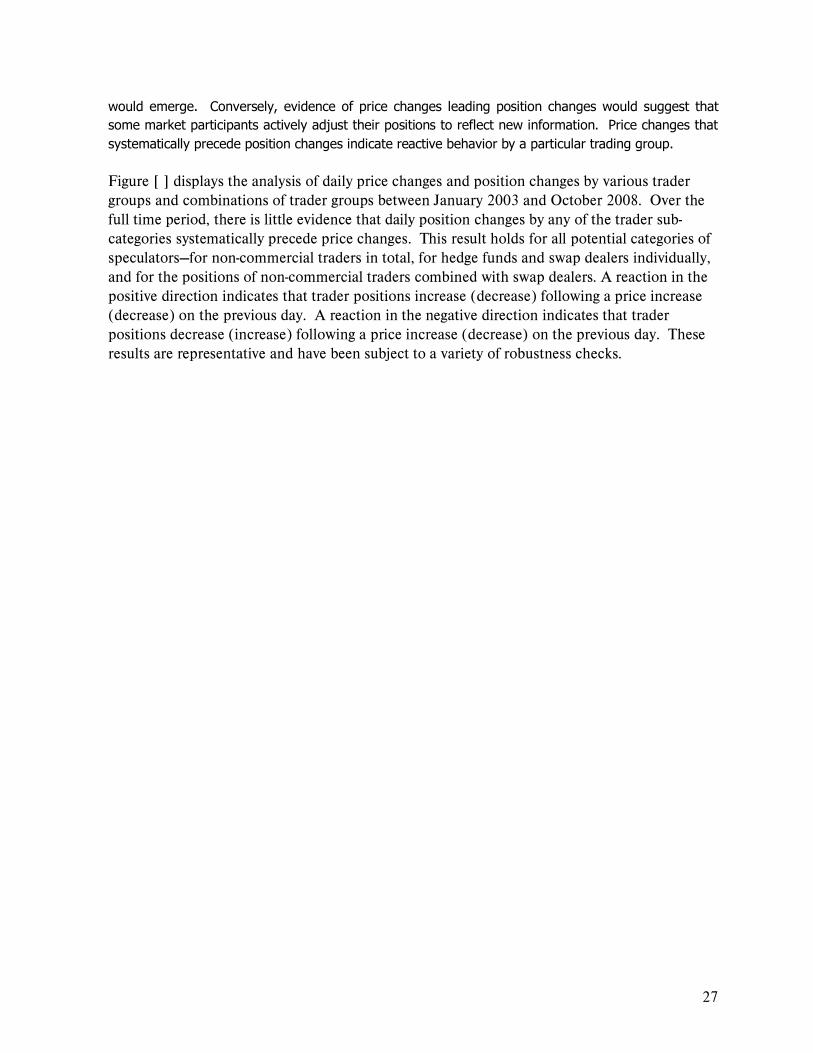
A well-established way to analyze the interaction between daily price changes and position changes is to examine directly whether various groups of traders change positions in advance of price changes.11 Intuitively, in order to realize gains from price changes, positions must be established prior to those price changes. Prices then may respond to those positions, or more precisely, the signal conveyed on establishing those positions. If specific trader categories were systematically establishing positions in advance of profitable price movements, then a pattern of position changes preceding price changes

11 The formal tests employed here are known as Granger Causality tests. A technical description of the tests is given in Appendix III. Granger causality tests were performed for different trader categories, over different holding periods, for different sample periods, in one and both directions. Trading activity in the nearby crude-oil contract averages about fifty percent of all trading activity and is a significant proportion of all open positions ranging from 18 to 30 percent of total open interest. Position changes are defined as changes in aggregated futures plus delta-adjusted options positions. Note that Granger Causality tests do not prove a causal relation between variables, only a statistical probability that, over a long enough period of time, one variable leads another.

27

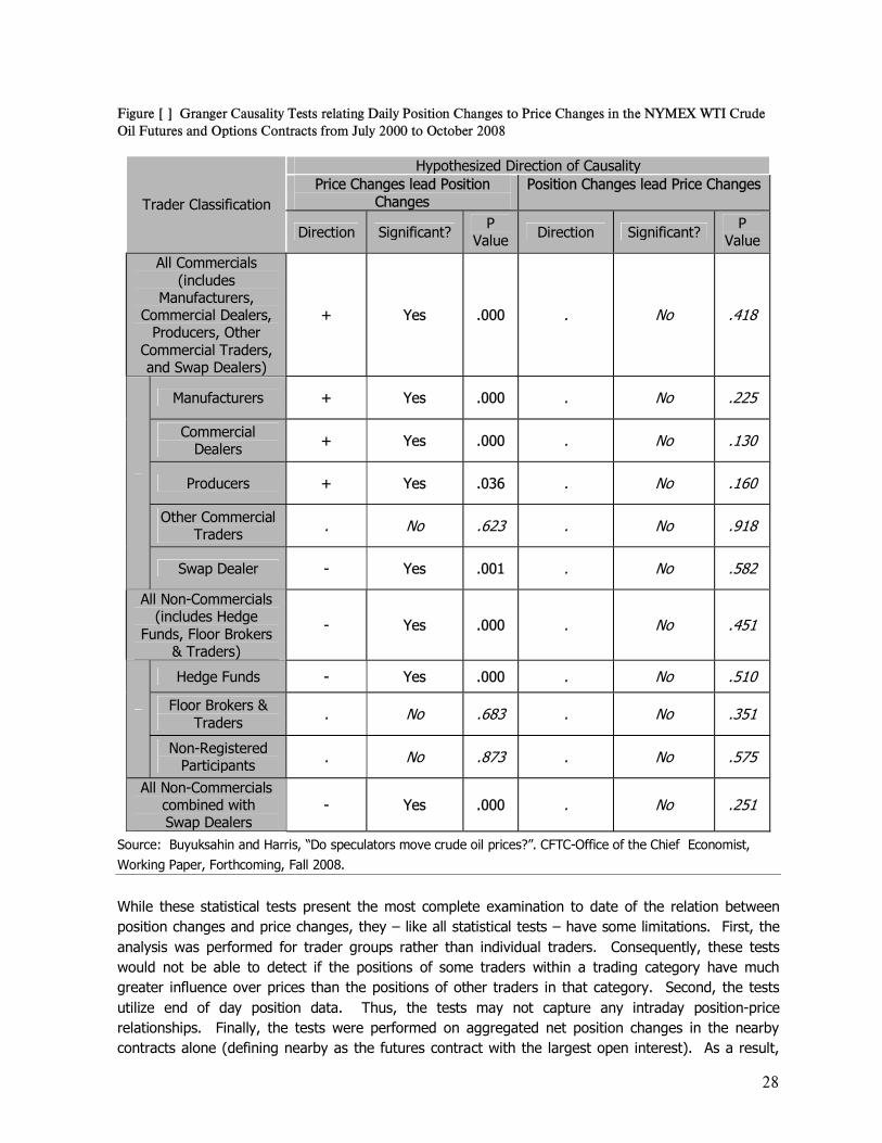
would emerge. Conversely, evidence of price changes leading position changes would suggest that some market participants actively adjust their positions to reflect new information. Price changes that systematically precede position changes indicate reactive behavior by a particular trading group. Figure [ ] displays the analysis of daily price changes and position changes by various trader groups and combinations of trader groups between January 2003 and October 2008. Over the full time period, there is little evidence that daily position changes by any of the trader sub-categories systematically precede price changes. This result holds for all potential categories of speculators�for non-commercial traders in total, for hedge funds and swap dealers individually, and for the positions of non-commercial traders combined with swap dealers. A reaction in the positive direction indicates that trader positions increase (decrease) following a price increase (decrease) on the previous day. A reaction in the negative direction indicates that trader positions decrease (increase) following a price increase (decrease) on the previous day. These results are representative and have been subject to a variety of robustness checks.

28

Figure [ ] Granger Causality Tests relating Daily Position Changes to Price Changes in the NYMEX WTI Crude Oil Futures and Options Contracts from July 2000 to October 2008

Hypothesized Direction of Causality Price Changes lead Position

Changes Position Changes lead Price Changes

Trader Classification

Direction Significant? P Value Direction Significant? P

Value All Commercials

(includes Manufacturers,

Commercial Dealers, Producers, Other

Commercial Traders, and Swap Dealers)

+ Yes .000 . No .418

Manufacturers + Yes .000 . No .225

Commercial Dealers + Yes .000 . No .130

Producers + Yes .036 . No .160

Other Commercial Traders . No .623 . No .918

Swap Dealer - Yes .001 . No .582

All Non-Commercials (includes Hedge

Funds, Floor Brokers & Traders)

- Yes .000 . No .451

Hedge Funds - Yes .000 . No .510

Floor Brokers & Traders . No .683 . No .351

Non-Registered Participants . No .873 . No .575

All Non-Commercials combined with Swap Dealers

- Yes .000 . No .251

Source: Buyuksahin and Harris, �Do speculators move crude oil prices?�. CFTC-Office of the Chief Economist, Working Paper, Forthcoming, Fall 2008.

While these statistical tests present the most complete examination to date of the relation between position changes and price changes, they � like all statistical tests � have some limitations. First, the analysis was performed for trader groups rather than individual traders. Consequently, these tests would not be able to detect if the positions of some traders within a trading category have much greater influence over prices than the positions of other traders in that category. Second, the tests utilize end of day position data. Thus, the tests may not capture any intraday position-price relationships. Finally, the tests were performed on aggregated net position changes in the nearby contracts alone (defining nearby as the futures contract with the largest open interest). As a result,

29

the tests do not reflect a systematic effect of position changes at different maturities on either the prices of the nearby futures contract or on the whole term structure of futures prices. That said, if the actions of particular groups of traders had systematically driven the recent oil price increases, the tests performed should have made it quite apparent. Again, it is useful to note that while the tests do not find that that changes in daily positions systematically lead changes in prices, such a finding would not necessarily imply that position changes were responsible for the price changes. Nevertheless, the lack of significant position changes leading price changes is informative. Taken as a whole, these tests are consistent with the view that current oil prices are being driven by fundamental supply and demand factors.

B. Select Agricultural Commodities - Corn, Wheat, and Soybeans

1. Background A number of long-term, slowly evolving trends have affected the global supply and demand for food commodities. The impact of these trends has been to slow growth in production and to strengthen demand. The resulting tightening of the global supply and demand balance has gradually put upward pressure on agricultural prices. Many of these long-term trends have been amplified by the more recent developments that have put additional upward pressure on world prices. These developments include rising energy costs, a series of policy changes in the United States and abroad, a weakening dollar, and changes in the profiles of commodity market participants.

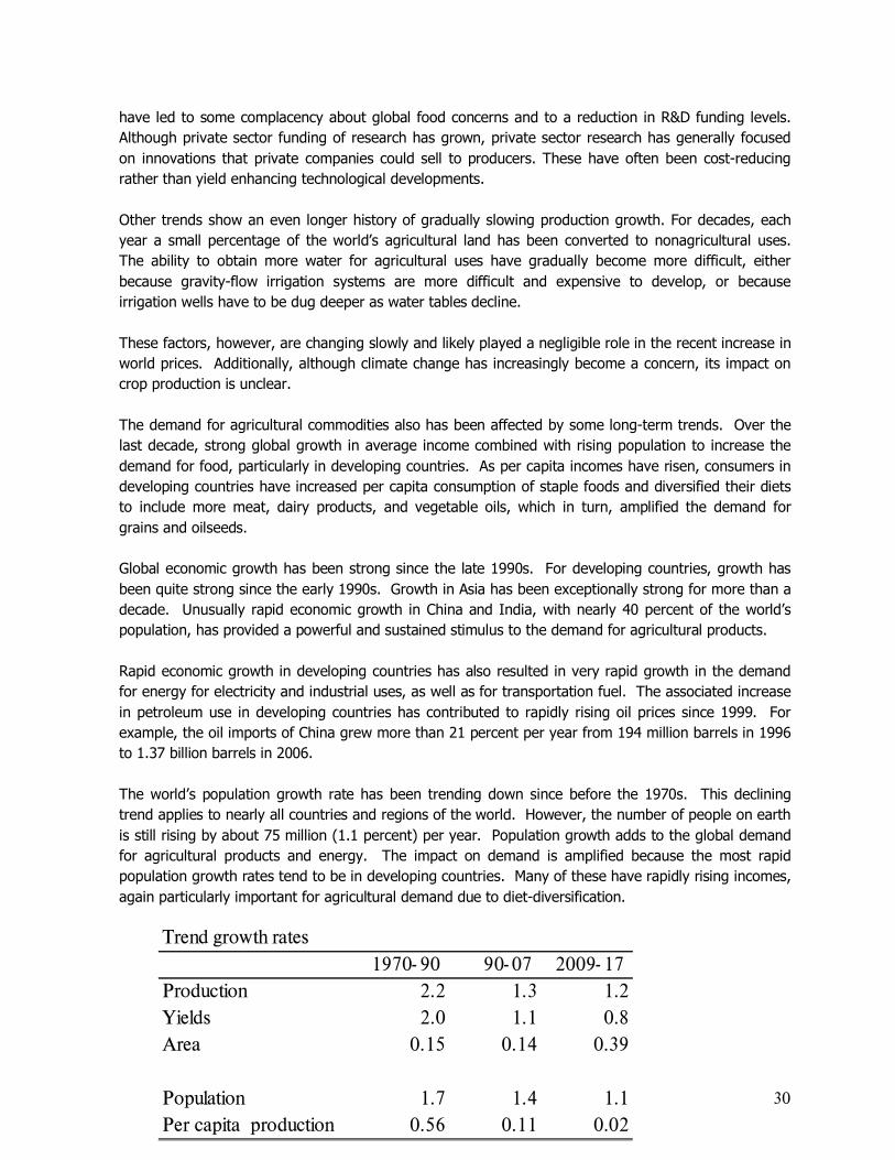
2. Long-Term Trends in Supply and Demand The annual growth rate of aggregate world grains and oilseeds production has been slowing. Between 1970 and 1990, production rose an average 2.2 percent per year. Since 1990, the growth rate has declined to about 1.3 percent. USDA projects this rate will decline to 1.2 percent per year between 2009 and 2017. Growth in productivity, measured in terms of average aggregate yield, has contributed much more to the growth in production globally than has expansion in the area planted to grains and oilseeds. Global aggregate yield growth averaged 2.0 percent per year from 1970 to 1990, but declined to 1.1 percent between 1990 and 2007. Yield growth is projected to continue declining over the next 10 years to less than 1.0 percent per year. The growth rate for area harvested has averaged only about 0.15 percent per year during the last 38 years. USDA projects that crop prices will remain strong during the next decade. The continued higher prices will provide the incentive for producers to respond by increasing the area allocated to crops. Some of this expanded area planted will come from land converted to cropland from non-cropland uses, such as pasture and forest. Area harvested also will increase as a result of more intensive use of existing cropland, generally from double-cropping and reduced fallow area. Reduced agricultural research and development by governmental and international institutions may have contributed to the slowing growth in crop yields. Stable food prices during the last two decades

30

have led to some complacency about global food concerns and to a reduction in R&D funding levels. Although private sector funding of research has grown, private sector research has generally focused on innovations that private companies could sell to producers. These have often been cost-reducing rather than yield enhancing technological developments. Other trends show an even longer history of gradually slowing production growth. For decades, each year a small percentage of the world�s agricultural land has been converted to nonagricultural uses. The ability to obtain more water for agricultural uses have gradually become more difficult, either because gravity-flow irrigation systems are more difficult and expensive to develop, or because irrigation wells have to be dug deeper as water tables decline. These factors, however, are changing slowly and likely played a negligible role in the recent increase in world prices. Additionally, although climate change has increasingly become a concern, its impact on crop production is unclear. The demand for agricultural commodities also has been affected by some long-term trends. Over the last decade, strong global growth in average income combined with rising population to increase the demand for food, particularly in developing countries. As per capita incomes have risen, consumers in developing countries have increased per capita consumption of staple foods and diversified their diets to include more meat, dairy products, and vegetable oils, which in turn, amplified the demand for grains and oilseeds. Global economic growth has been strong since the late 1990s. For developing countries, growth has been quite strong since the early 1990s. Growth in Asia has been exceptionally strong for more than a decade. Unusually rapid economic growth in China and India, with nearly 40 percent of the world�s population, has provided a powerful and sustained stimulus to the demand for agricultural products. Rapid economic growth in developing countries has also resulted in very rapid growth in the demand for energy for electricity and industrial uses, as well as for transportation fuel. The associated increase in petroleum use in developing countries has contributed to rapidly rising oil prices since 1999. For example, the oil imports of China grew more than 21 percent per year from 194 million barrels in 1996 to 1.37 billion barrels in 2006. The world�s population growth rate has been trending down since before the 1970s. This declining trend applies to nearly all countries and regions of the world. However, the number of people on earth is still rising by about 75 million (1.1 percent) per year. Population growth adds to the global demand for agricultural products and energy. The impact on demand is amplified because the most rapid population growth rates tend to be in developing countries. Many of these have rapidly rising incomes, again particularly important for agricultural demand due to diet-diversification.

Trend growth rates

1970- 90 90- 07 2009- 17

Production 2.2 1.3 1.2

Yields 2.0 1.1 0.8

Area 0.15 0.14 0.39

Population 1.7 1.4 1.1

Per capita production 0.56 0.11 0.02

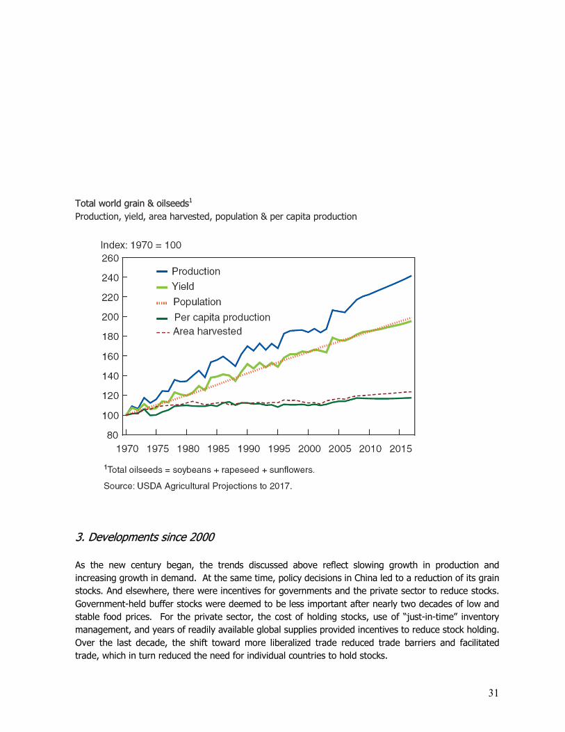
31

Total world grain & oilseeds1 Production, yield, area harvested, population & per capita production

3. Developments since 2000 As the new century began, the trends discussed above reflect slowing growth in production and increasing growth in demand. At the same time, policy decisions in China led to a reduction of its grain stocks. And elsewhere, there were incentives for governments and the private sector to reduce stocks. Government-held buffer stocks were deemed to be less important after nearly two decades of low and stable food prices. For the private sector, the cost of holding stocks, use of �just-in-time� inventory management, and years of readily available global supplies provided incentives to reduce stock holding. Over the last decade, the shift toward more liberalized trade reduced trade barriers and facilitated trade, which in turn reduced the need for individual countries to hold stocks.

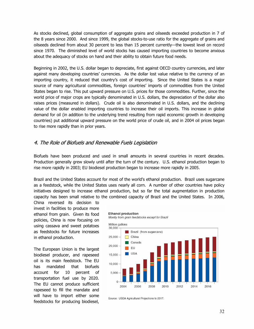
32

As stocks declined, global consumption of aggregate grains and oilseeds exceeded production in 7 of the 8 years since 2000. And since 1999, the global stocks-to-use ratio for the aggregate of grains and oilseeds declined from about 30 percent to less than 15 percent currently�the lowest level on record since 1970. The diminished level of world stocks has caused importing countries to become anxious about the adequacy of stocks on hand and their ability to obtain future food needs. Beginning in 2002, the U.S. dollar began to depreciate, first against OECD country currencies, and later against many developing countries� currencies. As the dollar lost value relative to the currency of an importing country, it reduced that country�s cost of importing. Since the United States is a major source of many agricultural commodities, foreign countries� imports of commodities from the United States began to rise. This put upward pressure on U.S. prices for those commodities. Further, since the world price of major crops are typically denominated in U.S. dollars, the depreciation of the dollar also raises prices (measured in dollars). Crude oil is also denominated in U.S. dollars, and the declining value of the dollar enabled importing countries to increase their oil imports. This increase in global demand for oil (in addition to the underlying trend resulting from rapid economic growth in developing countries) put additional upward pressure on the world price of crude oil, and in 2004 oil prices began to rise more rapidly than in prior years.

4. The Role of Biofuels and Renewable Fuels Legislation Biofuels have been produced and used in small amounts in several countries in recent decades. Production generally grew slowly until after the turn of the century. U.S. ethanol production began to rise more rapidly in 2003; EU biodiesel production began to increase more rapidly in 2005. Brazil and the United States account for most of the world�s ethanol production. Brazil uses sugarcane as a feedstock, while the United States uses nearly all corn. A number of other countries have policy initiatives designed to increase ethanol production, but so far the total augmentation in production capacity has been small relative to the combined capacity of Brazil and the United States. In 2006, China reversed its decision to invest in facilities to produce more ethanol from grain. Given its food policies, China is now focusing on using cassava and sweet potatoes as feedstocks for future increases in ethanol production. The European Union is the largest biodiesel producer, and rapeseed oil is its main feedstock. The EU has mandated that biofuels account for 10 percent of transportation fuel use by 2020. The EU cannot produce sufficient rapeseed to fill the mandate and will have to import either some feedstocks for producing biodiesel,

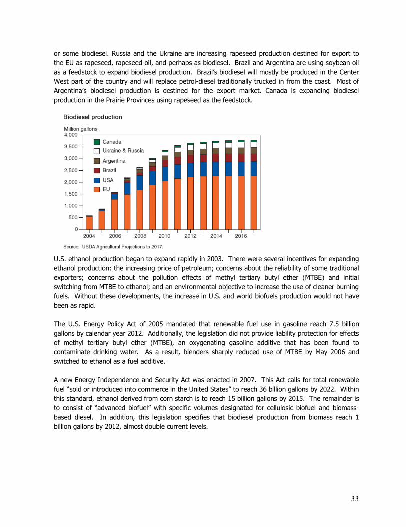
33

or some biodiesel. Russia and the Ukraine are increasing rapeseed production destined for export to the EU as rapeseed, rapeseed oil, and perhaps as biodiesel. Brazil and Argentina are using soybean oil as a feedstock to expand biodiesel production. Brazil�s biodiesel will mostly be produced in the Center West part of the country and will replace petrol-diesel traditionally trucked in from the coast. Most of Argentina�s biodiesel production is destined for the export market. Canada is expanding biodiesel production in the Prairie Provinces using rapeseed as the feedstock.

U.S. ethanol production began to expand rapidly in 2003. There were several incentives for expanding ethanol production: the increasing price of petroleum; concerns about the reliability of some traditional exporters; concerns about the pollution effects of methyl tertiary butyl ether (MTBE) and initial switching from MTBE to ethanol; and an environmental objective to increase the use of cleaner burning fuels. Without these developments, the increase in U.S. and world biofuels production would not have been as rapid. The U.S. Energy Policy Act of 2005 mandated that renewable fuel use in gasoline reach 7.5 billion gallons by calendar year 2012. Additionally, the legislation did not provide liability protection for effects of methyl tertiary butyl ether (MTBE), an oxygenating gasoline additive that has been found to contaminate drinking water. As a result, blenders sharply reduced use of MTBE by May 2006 and switched to ethanol as a fuel additive. A new Energy Independence and Security Act was enacted in 2007. This Act calls for total renewable fuel �sold or introduced into commerce in the United States� to reach 36 billion gallons by 2022. Within this standard, ethanol derived from corn starch is to reach 15 billion gallons by 2015. The remainder is to consist of �advanced biofuel� with specific volumes designated for cellulosic biofuel and biomass-based diesel. In addition, this legislation specifies that biodiesel production from biomass reach 1 billion gallons by 2012, almost double current levels.

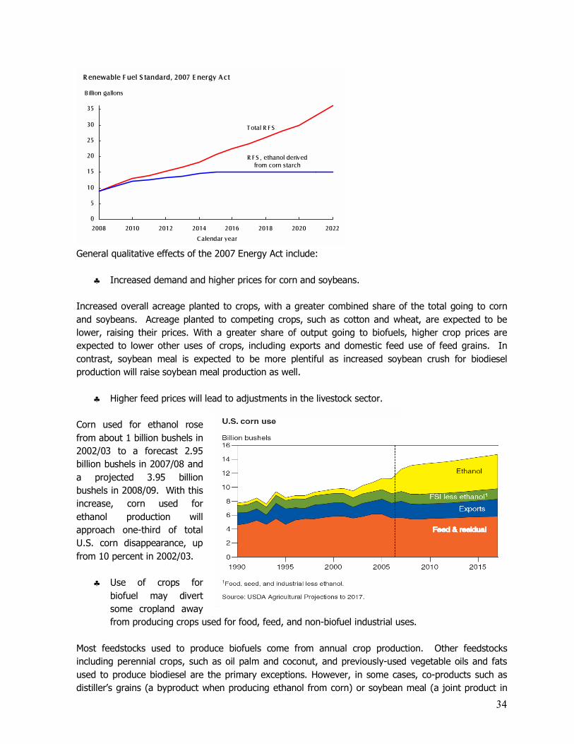
34

0

5

10

15

20

25

30

35

2008 2010 2012 2014 2016 2018 2020 2022

B illion gallons

R enewable F uel S tandard, 2007 E nergy A c t

C alendar year

T otal R F S

R F S , ethanol derived from corn starch

General qualitative effects of the 2007 Energy Act include:

♣ Increased demand and higher prices for corn and soybeans. Increased overall acreage planted to crops, with a greater combined share of the total going to corn and soybeans. Acreage planted to competing crops, such as cotton and wheat, are expected to be lower, raising their prices. With a greater share of output going to biofuels, higher crop prices are expected to lower other uses of crops, including exports and domestic feed use of feed grains. In contrast, soybean meal is expected to be more plentiful as increased soybean crush for biodiesel production will raise soybean meal production as well.

♣ Higher feed prices will lead to adjustments in the livestock sector. Corn used for ethanol rose from about 1 billion bushels in 2002/03 to a forecast 2.95 billion bushels in 2007/08 and a projected 3.95 billion bushels in 2008/09. With this increase, corn used for ethanol production will approach one-third of total U.S. corn disappearance, up from 10 percent in 2002/03.

♣ Use of crops for biofuel may divert some cropland away from producing crops used for food, feed, and non-biofuel industrial uses.

Most feedstocks used to produce biofuels come from annual crop production. Other feedstocks including perennial crops, such as oil palm and coconut, and previously-used vegetable oils and fats used to produce biodiesel are the primary exceptions. However, in some cases, co-products such as distiller�s grains (a byproduct when producing ethanol from corn) or soybean meal (a joint product in

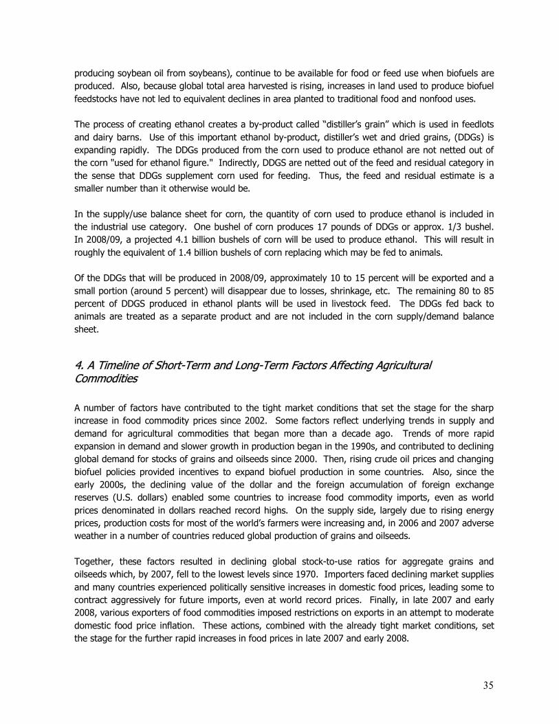
35

producing soybean oil from soybeans), continue to be available for food or feed use when biofuels are produced. Also, because global total area harvested is rising, increases in land used to produce biofuel feedstocks have not led to equivalent declines in area planted to traditional food and nonfood uses. The process of creating ethanol creates a by-product called �distiller�s grain� which is used in feedlots and dairy barns. Use of this important ethanol by-product, distiller�s wet and dried grains, (DDGs) is expanding rapidly. The DDGs produced from the corn used to produce ethanol are not netted out of the corn "used for ethanol figure." Indirectly, DDGS are netted out of the feed and residual category in the sense that DDGs supplement corn used for feeding. Thus, the feed and residual estimate is a smaller number than it otherwise would be. In the supply/use balance sheet for corn, the quantity of corn used to produce ethanol is included in the industrial use category. One bushel of corn produces 17 pounds of DDGs or approx. 1/3 bushel. In 2008/09, a projected 4.1 billion bushels of corn will be used to produce ethanol. This will result in roughly the equivalent of 1.4 billion bushels of corn replacing which may be fed to animals. Of the DDGs that will be produced in 2008/09, approximately 10 to 15 percent will be exported and a small portion (around 5 percent) will disappear due to losses, shrinkage, etc. The remaining 80 to 85 percent of DDGS produced in ethanol plants will be used in livestock feed. The DDGs fed back to animals are treated as a separate product and are not included in the corn supply/demand balance sheet.

4. A Timeline of Short-Term and Long-Term Factors Affecting Agricultural Commodities A number of factors have contributed to the tight market conditions that set the stage for the sharp increase in food commodity prices since 2002. Some factors reflect underlying trends in supply and demand for agricultural commodities that began more than a decade ago. Trends of more rapid expansion in demand and slower growth in production began in the 1990s, and contributed to declining global demand for stocks of grains and oilseeds since 2000. Then, rising crude oil prices and changing biofuel policies provided incentives to expand biofuel production in some countries. Also, since the early 2000s, the declining value of the dollar and the foreign accumulation of foreign exchange reserves (U.S. dollars) enabled some countries to increase food commodity imports, even as world prices denominated in dollars reached record highs. On the supply side, largely due to rising energy prices, production costs for most of the world�s farmers were increasing and, in 2006 and 2007 adverse weather in a number of countries reduced global production of grains and oilseeds. Together, these factors resulted in declining global stock-to-use ratios for aggregate grains and oilseeds which, by 2007, fell to the lowest levels since 1970. Importers faced declining market supplies and many countries experienced politically sensitive increases in domestic food prices, leading some to contract aggressively for future imports, even at world record prices. Finally, in late 2007 and early 2008, various exporters of food commodities imposed restrictions on exports in an attempt to moderate domestic food price inflation. These actions, combined with the already tight market conditions, set the stage for the further rapid increases in food prices in late 2007 and early 2008.

36

5. Analysis of Fundamental Factors in Relation to Prices

5. Analysis of Fundamental Factors in Relation to Prices Commodity Stocks and Prices. Fundamental market analysis of agricultural commodities, such as field crops, relies extensively on a supply and use balance sheet approach to assess the effects supply and demand on price. In a balance sheet, supplies are the sum of beginning stocks (carryover from the previous year), plus production, and imports. Use serves as an indicator of demand with various categories of domestic disappearance depending upon the commodity and its uses. Using corn as an example, domestic use includes food, seed, and industrial use (including ethanol), feed, and residual use. Total use is the combination of domestic disappearance plus exports. The sum of supplies minus the sum of uses results in ending stocks that will be carried forward into the new marketing year. Balance sheet analysis is a fairly straight forward way to quantify the interaction between supply and demand. For seasonally produced and storable commodities, physical inventories at the end of the marketing year are an important indicator of the balance between supplies and demand. Ending stocks, or carryover, have a negative correlation with price. When considered in relation to demand and calculated as the ratio of stocks-to-use, the relationship to price can be shown as a downward sloping non-linear curve with the highest prices observed when the stocks-to-use ratio is lowest. As use rises relative to supply, the stocks-to-use ratio declines and prices rise. Conversely, as supplies rise relative to use, the stocks-to-use ratio increases and prices fall. Corn. The historic relationship between stocks-to-use and prices for corn fits this analytic framework very well. As the dominant U.S. field crop with more acreage and higher production than either wheat or soybeans, corn tends to drive prices for the other grains and oilseeds. Prices for corn began to rise

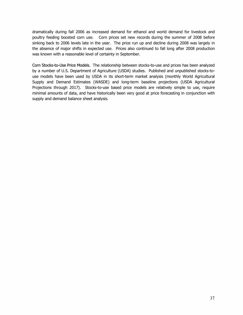
37

dramatically during fall 2006 as increased demand for ethanol and world demand for livestock and poultry feeding boosted corn use. Corn prices set new records during the summer of 2008 before sinking back to 2006 levels late in the year. The price run up and decline during 2008 was largely in the absence of major shifts in expected use. Prices also continued to fall long after 2008 production was known with a reasonable level of certainty in September. Corn Stocks-to-Use Price Models. The relationship between stocks-to-use and prices has been analyzed by a number of U.S. Department of Agriculture (USDA) studies. Published and unpublished stocks-to-use models have been used by USDA in its short-term market analysis (monthly World Agricultural Supply and Demand Estimates (WASDE) and long-term baseline projections (USDA Agricultural Projections through 2017). Stocks-to-use based price models are relatively simple to use, require minimal amounts of data, and have historically been very good at price forecasting in conjunction with supply and demand balance sheet analysis.

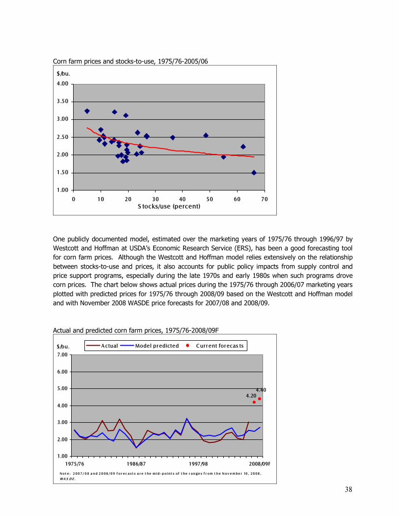
38

Corn farm prices and stocks-to-use, 1975/76-2005/06

1.00

1.50

2.00

2.50

3.00

3.50

4.00

0 10 20 30 40 50 60 70S tocks/use (percent)

$/bu.

One publicly documented model, estimated over the marketing years of 1975/76 through 1996/97 by Westcott and Hoffman at USDA�s Economic Research Service (ERS), has been a good forecasting tool for corn farm prices. Although the Westcott and Hoffman model relies extensively on the relationship between stocks-to-use and prices, it also accounts for public policy impacts from supply control and price support programs, especially during the late 1970s and early 1980s when such programs drove corn prices. The chart below shows actual prices during the 1975/76 through 2006/07 marketing years plotted with predicted prices for 1975/76 through 2008/09 based on the Westcott and Hoffman model and with November 2008 WASDE price forecasts for 2007/08 and 2008/09. Actual and predicted corn farm prices, 1975/76-2008/09F

4.204.40

1.00

2.00

3.00

4.00

5.00

6.00

7.00

1975/76 1986/87 1997/98 2008/09F

$/bu. A ctual Model pr edicted C ur r ent for ecas ts

N o t e : 2 0 0 7 / 0 8 a n d 2 0 0 8 / 0 9 f o r e c a s t s a r e t he m i d - p o i n t s o f t he r a n g e s f r om t h e N o v e m b e r 10 , 2 0 0 8 ,

W A S D E .

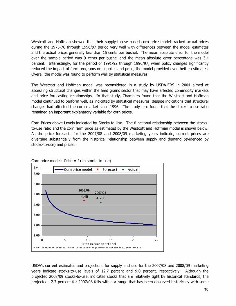
39

Westcott and Hoffman showed that their supply-to-use based corn price model tracked actual prices during the 1975-76 through 1996/97 period very well with differences between the model estimates and the actual prices generally less than 15 cents per bushel. The mean absolute error for the model over the sample period was 9 cents per bushel and the mean absolute error percentage was 3.4 percent. Interestingly, for the period of 1991/92 through 1996/97, when policy changes significantly reduced the impact of farm programs on supplies and price, the model provided even better estimates. Overall the model was found to perform well by statistical measures. The Westcott and Hoffman model was reconsidered in a study by USDA-ERS in 2004 aimed at assessing structural changes within the feed grains sector that may have affected commodity markets and price forecasting relationships. In that study, Chambers found that the Westcott and Hoffman model continued to perform well, as indicated by statistical measures, despite indications that structural changes had affected the corn market since 1996. The study also found that the stocks-to-use ratio remained an important explanatory variable for corn prices. Corn Prices above Levels indicated by Stocks-to-Use. The functional relationship between the stocks-to-use ratio and the corn farm price as estimated by the Westcott and Hoffman model is shown below. As the price forecasts for the 2007/08 and 2008/09 marketing years indicate, current prices are diverging substantially from the historical relationship between supply and demand (evidenced by stocks-to-use) and prices. Corn price model: Price = f (Ln stocks-to-use)

4.40 4.20

1.00

2.00

3.00

4.00

5.00

6.00

7.00

0 5 10 15 20 25S tocks /us e (percent)

$/bu. Corn pr ic e model Forec as t Ac tual

2008/092007/08

N ot e : 2 0 0 8 / 0 9 f o r e c a s t i s t h e m i d - p o i n t o f t he r a n g e f r o m t h e N ov e mb e r 10 , 2 0 0 8 , W A S D E .

USDA�s current estimates and projections for supply and use for the 2007/08 and 2008/09 marketing years indicate stocks-to-use levels of 12.7 percent and 9.0 percent, respectively. Although the projected 2008/09 stocks-to-use, indicates stocks that are relatively tight by historical standards, the projected 12.7 percent for 2007/08 falls within a range that has been observed historically with some

40

frequency. In both cases, expected prices are sharply higher than would be explained by the historical relationship between stocks-to-use and price. The frequently repeated explanation for the dramatic rise in corn prices is increased demand for corn for ethanol. Recent work by USDA and the fundamental logic behind balance sheet analysis brings into question this overly simplistic view. The Trostle analysis released by USDA-ERS in May 2008 indicated that a number of factors are driving the prices of grains and oilseeds higher. Among the factors indicated were rising global demand from livestock and poultry feeding, the declining value of the dollar, rising energy prices, increasing costs of production, growing foreign-exchange holdings by major food-importing countries, and trade restrictive policies implemented by some countries to shut off exports and dampen domestic price increases. Also raised as an issue was increased involvement in futures markets by hedge funds, index funds, and sovereign wealth funds. Although demand for biofuels has contributed to increased demand for grains and oilseeds, expansion in crop area world wide has far surpassed the area needed to support expanded biofuels production. Global harvested area for grains, annual oilseeds, and cotton increased 45 million acres between 2004 and 2007. Increased demand for biofuels feedstocks during these years, including corn for ethanol and vegetable oil for biodiesel, required only 11 million acres, or 24 percent of this area increase. Increased use of corn for ethanol has boosted demand for corn in the United States, but the logic of balance sheet analysis should capture this impact through the stocks-to-use ratio which has been declining since the 2004/05 marketing year. Corn supplies have also risen sharply in recent years. In response to rising prices, U.S. farmers expanded corn plantings for 2007/08 by 15.3 million acres to 93.6 million, the highest planted area since 1944. At 2007 yields, this additional area boosted production 2.1 billion bushels, far surpassing the year-to-year increase in ethanol corn use estimated at 907 million bushels. These increases in supplies are also captured in the balance sheet and reflected in ending stocks. The sharp rise in corn prices starting in March 2008 reflected reduced prospects for 2008/09 corn production. Producers indicated in March that they intended to plant less corn area this spring as a result of more attractive soybean prices and relative returns per acre. Corn prices continued to rally through the spring as persistent rains and cool temperatures delayed planting and crop emergence in April and May. Excessive rainfall further eroded the outlook for production during June, with significant losses to flooding and reduced yield prospects with replanting. Throughout this period 2008/09 supply and demand estimates published by USDA reflected these changes through adjustments to corn area and yields with accompanying adjustments to supplies and use. Despite these adjustments to the projected balance sheet, cash, forward, and futures prices continue to indicate farm price levels for 2007/08 and 2008/09 that exceed those predicted by the historical stocks-to-use relationship. USDA forecasts for 2007/08 and 2008/09 farm corn prices suggest that the curve depicting the relationship between stocks-to-use and price has shifted upward and to the right. Although the 2008/009 forecast reflects assumptions about the coming year�s balance sheet and past, as well as future pricing opportunities, the 2007/08 forecast is a final estimate reported by USDA�s National Agricultural Statistics Service. Using these forecasts for guidance suggests the curve shown below.

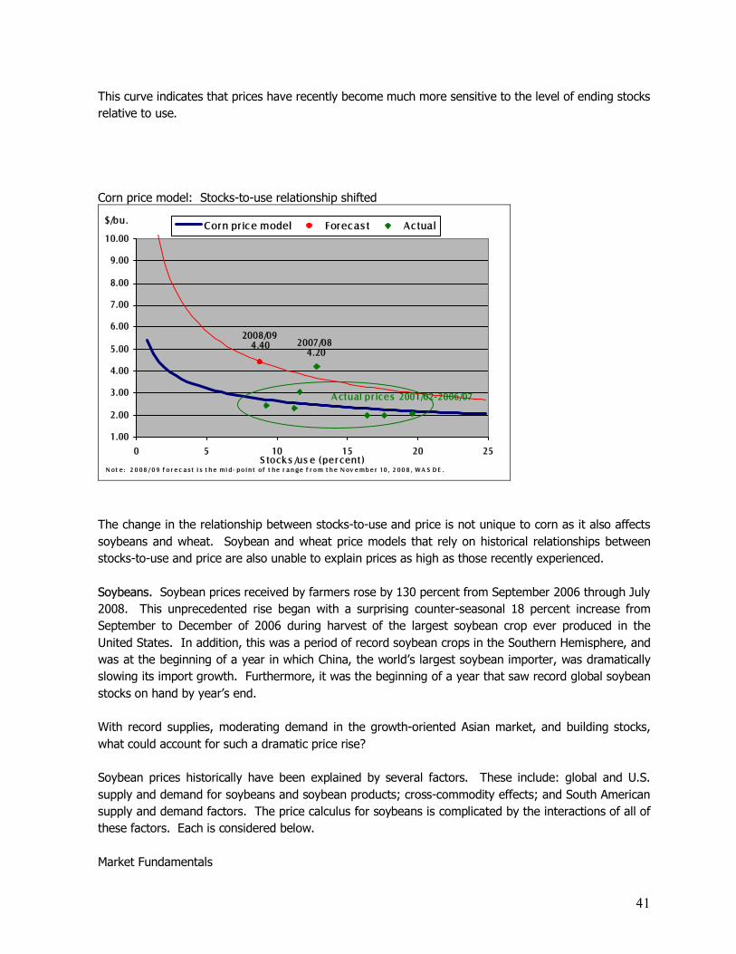
41

This curve indicates that prices have recently become much more sensitive to the level of ending stocks relative to use. Corn price model: Stocks-to-use relationship shifted

4.404.20

1.00

2.00

3.00

4.00

5.00

6.00

7.00

8.00

9.00

10.00

0 5 10 15 20 25S tock s /us e (per cent)

$/bu. Corn pr ic e model Forec as t Actual

2008/092007/08

N ot e : 2 0 0 8 / 0 9 f o r e c a s t i s t h e m i d - p o i n t o f t he r a n g e f r o m t h e N ov e mb e r 10 , 2 0 0 8 , W A S D E .

A ctual pr ices 2001/02-2006/07

The change in the relationship between stocks-to-use and price is not unique to corn as it also affects soybeans and wheat. Soybean and wheat price models that rely on historical relationships between stocks-to-use and price are also unable to explain prices as high as those recently experienced. Soybeans. Soybean prices received by farmers rose by 130 percent from September 2006 through July 2008. This unprecedented rise began with a surprising counter-seasonal 18 percent increase from September to December of 2006 during harvest of the largest soybean crop ever produced in the United States. In addition, this was a period of record soybean crops in the Southern Hemisphere, and was at the beginning of a year in which China, the world�s largest soybean importer, was dramatically slowing its import growth. Furthermore, it was the beginning of a year that saw record global soybean stocks on hand by year�s end. With record supplies, moderating demand in the growth-oriented Asian market, and building stocks, what could account for such a dramatic price rise? Soybean prices historically have been explained by several factors. These include: global and U.S. supply and demand for soybeans and soybean products; cross-commodity effects; and South American supply and demand factors. The price calculus for soybeans is complicated by the interactions of all of these factors. Each is considered below. Market Fundamentals

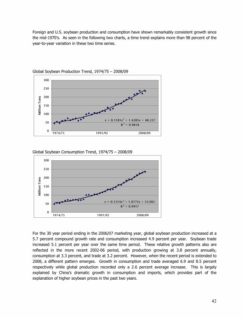
42

Foreign and U.S. soybean production and consumption have shown remarkably consistent growth since the mid-1970�s. As seen in the following two charts, a time trend explains more than 98 percent of the year-to-year variation in these two time series. Global Soybean Production Trend, 1974/75 � 2008/09

y = 0.1181x2 + 1.4285x + 48.237

R 2 = 0.9818

0

50

100

150

200

250

300

Mil

lio

n T

on

s

1974/75 2008/091991/92

Global Soybean Consumption Trend, 1974/75 � 2008/09

y = 0.1214x 2 + 1.0775x + 53.061

R 2 = 0.9917

0

50

100

150

200

250

300

Mil

lio

n T

on

s

1974/75 2008/091991/92 For the 30 year period ending in the 2006/07 marketing year, global soybean production increased at a 5.7 percent compound growth rate and consumption increased 4.9 percent per year. Soybean trade increased 5.1 percent per year over the same time period. These relative growth patterns also are reflected in the more recent 2002-06 period, with production growing at 3.8 percent annually, consumption at 3.3 percent, and trade at 3.2 percent. However, when the recent period is extended to 2008, a different pattern emerges. Growth in consumption and trade averaged 6.9 and 8.5 percent respectively while global production recorded only a 2.6 percent average increase. This is largely explained by China�s dramatic growth in consumption and imports, which provides part of the explanation of higher soybean prices in the past two years.

43

Despite the recent shift to higher consumption growth rates relative to production, global soybean stocks relative to use remain near long-run historical average levels. The following chart shows global stocks relative to use.

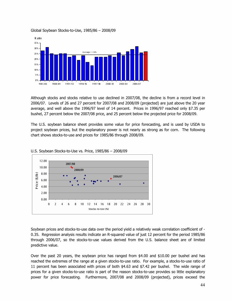
44

Global Soybean Stocks-to-Use, 1985/86 � 2008/09

0%

5%

10%

15%

20%

25%

30%

35%

1985-86 1988-89 1991-92 1994- 95 1997- 98 2000- 01 2003-04 2006-07

R atio

Ave rage = 2 4%

Although stocks and stocks relative to use declined in 2007/08, the decline is from a record level in 2006/07. Levels of 26 and 27 percent for 2007/08 and 2008/09 (projected) are just above the 20 year average, and well above the 1996/97 level of 14 percent. Prices in 1996/97 reached only $7.35 per bushel, 27 percent below the 2007/08 price, and 25 percent below the projected price for 2008/09. The U.S. soybean balance sheet provides some value for price forecasting, and is used by USDA to project soybean prices, but the explanatory power is not nearly as strong as for corn. The following chart shows stocks-to-use and prices for 1985/86 through 2008/09. U.S. Soybean Stocks-to-Use vs. Price, 1985/86 � 2008/09

0.00

2.00

4.00

6.00

8.00

10.00

12.00

0 2 4 6 8 10 12 14 16 18 20 22 24 26 28 30

S tocks - to-Us e (%)

Pri

ce (

$/lb

)

2008/09

2006/07

2007/08

Soybean prices and stocks-to-use data over the period yield a relatively weak correlation coefficient of -0.35. Regression analysis results indicate an R-squared value of just 12 percent for the period 1985/86 through 2006/07, so the stocks-to-use values derived from the U.S. balance sheet are of limited predictive value. Over the past 20 years, the soybean price has ranged from $4.00 and $10.00 per bushel and has reached the extremes of the range at a given stocks-to-use ratio. For example, a stocks-to-use ratio of 11 percent has been associated with prices of both $4.63 and $7.42 per bushel. The wide range of prices for a given stocks-to-use ratio is part of the reason stocks-to-use provides so little explanatory power for price forecasting. Furthermore, 2007/08 and 2008/09 (projected), prices exceed the

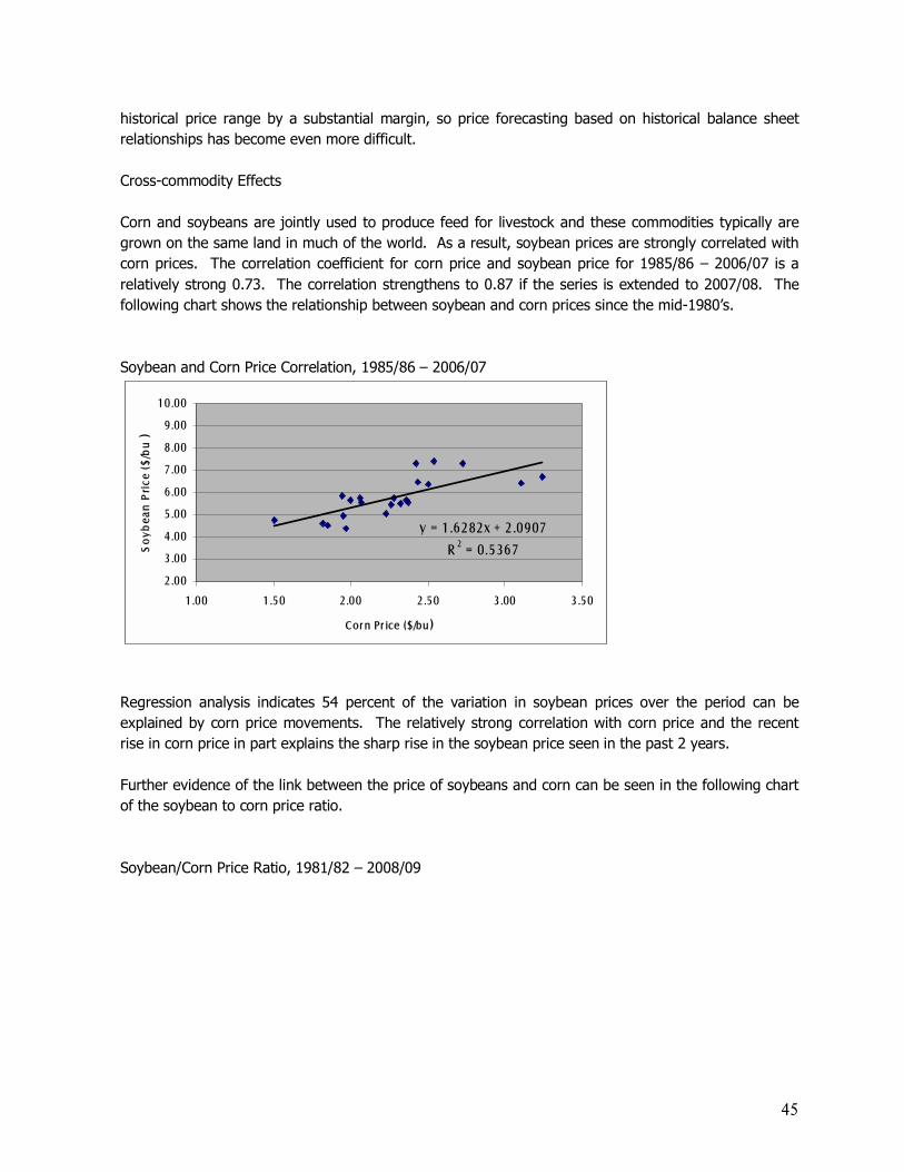
45

historical price range by a substantial margin, so price forecasting based on historical balance sheet relationships has become even more difficult. Cross-commodity Effects Corn and soybeans are jointly used to produce feed for livestock and these commodities typically are grown on the same land in much of the world. As a result, soybean prices are strongly correlated with corn prices. The correlation coefficient for corn price and soybean price for 1985/86 � 2006/07 is a relatively strong 0.73. The correlation strengthens to 0.87 if the series is extended to 2007/08. The following chart shows the relationship between soybean and corn prices since the mid-1980�s. Soybean and Corn Price Correlation, 1985/86 � 2006/07

y = 1.6282x + 2.0907

R 2 = 0.5367

2.00

3.00

4.00

5.00

6.00

7.00

8.00

9.00

10.00

1.00 1.50 2.00 2.50 3.00 3.50

C or n Pr ice ($/bu)

So

ybea

n P

rice

($/

bu

)

Regression analysis indicates 54 percent of the variation in soybean prices over the period can be explained by corn price movements. The relatively strong correlation with corn price and the recent rise in corn price in part explains the sharp rise in the soybean price seen in the past 2 years. Further evidence of the link between the price of soybeans and corn can be seen in the following chart of the soybean to corn price ratio. Soybean/Corn Price Ratio, 1981/82 � 2008/09

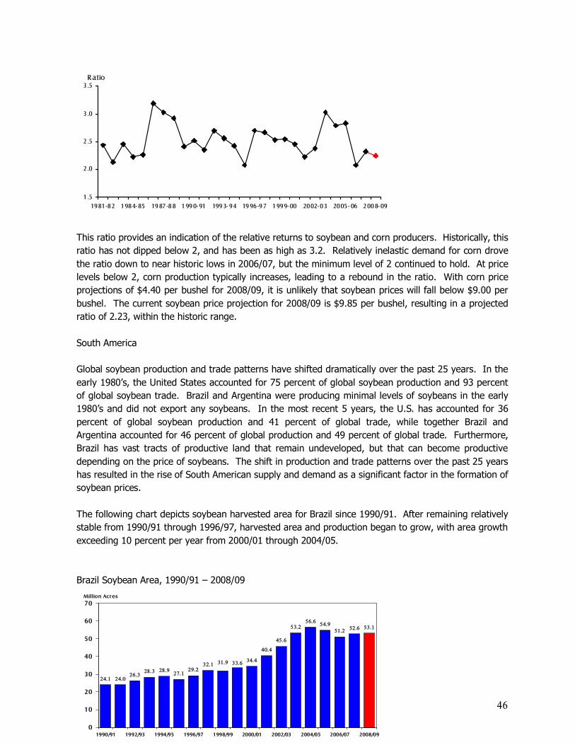
46

1.5

2.0

2.5

3.0

3.5

1981-82 1984- 85 1987 -88 1990- 91 1993- 94 1996-97 1999- 00 2002- 03 2005- 06 2008- 09

Ratio

This ratio provides an indication of the relative returns to soybean and corn producers. Historically, this ratio has not dipped below 2, and has been as high as 3.2. Relatively inelastic demand for corn drove the ratio down to near historic lows in 2006/07, but the minimum level of 2 continued to hold. At price levels below 2, corn production typically increases, leading to a rebound in the ratio. With corn price projections of $4.40 per bushel for 2008/09, it is unlikely that soybean prices will fall below $9.00 per bushel. The current soybean price projection for 2008/09 is $9.85 per bushel, resulting in a projected ratio of 2.23, within the historic range. South America Global soybean production and trade patterns have shifted dramatically over the past 25 years. In the early 1980�s, the United States accounted for 75 percent of global soybean production and 93 percent of global soybean trade. Brazil and Argentina were producing minimal levels of soybeans in the early 1980�s and did not export any soybeans. In the most recent 5 years, the U.S. has accounted for 36 percent of global soybean production and 41 percent of global trade, while together Brazil and Argentina accounted for 46 percent of global production and 49 percent of global trade. Furthermore, Brazil has vast tracts of productive land that remain undeveloped, but that can become productive depending on the price of soybeans. The shift in production and trade patterns over the past 25 years has resulted in the rise of South American supply and demand as a significant factor in the formation of soybean prices. The following chart depicts soybean harvested area for Brazil since 1990/91. After remaining relatively stable from 1990/91 through 1996/97, harvested area and production began to grow, with area growth exceeding 10 percent per year from 2000/01 through 2004/05. Brazil Soybean Area, 1990/91 � 2008/09

24.1 24.026.3

28.3 28.927.1

29.232.1

34.4

40.4

53.256.6

54.951.2 52.6 53.1

33.631.9

45.6

0

10

20

30

40

50

60

70

1990/91 1992/93 1994/95 1996/97 1998/99 2000/01 2002/03 2004/05 2006/07 2008/09

Million Acres

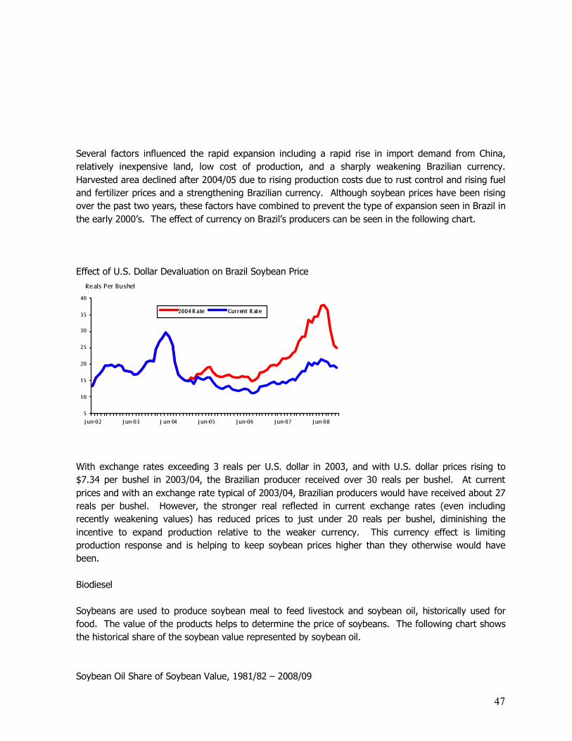
47

Several factors influenced the rapid expansion including a rapid rise in import demand from China, relatively inexpensive land, low cost of production, and a sharply weakening Brazilian currency. Harvested area declined after 2004/05 due to rising production costs due to rust control and rising fuel and fertilizer prices and a strengthening Brazilian currency. Although soybean prices have been rising over the past two years, these factors have combined to prevent the type of expansion seen in Brazil in the early 2000�s. The effect of currency on Brazil�s producers can be seen in the following chart. Effect of U.S. Dollar Devaluation on Brazil Soybean Price

5

10

15

20

25

30

35

40

J un-02 J un-03 J un- 04 J un-05 J un-06 J un-07 J un-08

Reals Per Bushel

2004 R ate Current R ate

With exchange rates exceeding 3 reals per U.S. dollar in 2003, and with U.S. dollar prices rising to $7.34 per bushel in 2003/04, the Brazilian producer received over 30 reals per bushel. At current prices and with an exchange rate typical of 2003/04, Brazilian producers would have received about 27 reals per bushel. However, the stronger real reflected in current exchange rates (even including recently weakening values) has reduced prices to just under 20 reals per bushel, diminishing the incentive to expand production relative to the weaker currency. This currency effect is limiting production response and is helping to keep soybean prices higher than they otherwise would have been. Biodiesel Soybeans are used to produce soybean meal to feed livestock and soybean oil, historically used for food. The value of the products helps to determine the price of soybeans. The following chart shows the historical share of the soybean value represented by soybean oil. Soybean Oil Share of Soybean Value, 1981/82 � 2008/09

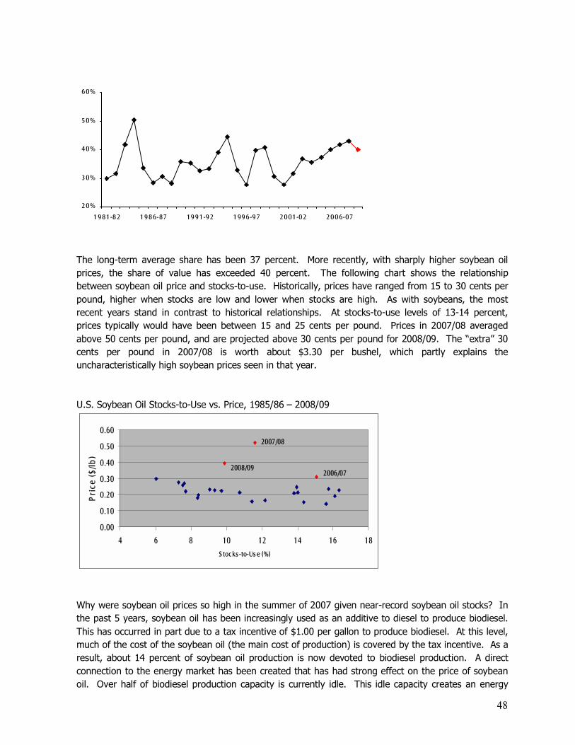
48

The long-term average share has been 37 percent. More recently, with sharply higher soybean oil prices, the share of value has exceeded 40 percent. The following chart shows the relationship between soybean oil price and stocks-to-use. Historically, prices have ranged from 15 to 30 cents per pound, higher when stocks are low and lower when stocks are high. As with soybeans, the most recent years stand in contrast to historical relationships. At stocks-to-use levels of 13-14 percent, prices typically would have been between 15 and 25 cents per pound. Prices in 2007/08 averaged above 50 cents per pound, and are projected above 30 cents per pound for 2008/09. The �extra� 30 cents per pound in 2007/08 is worth about $3.30 per bushel, which partly explains the uncharacteristically high soybean prices seen in that year. U.S. Soybean Oil Stocks-to-Use vs. Price, 1985/86 � 2008/09

0.00

0.10

0.20

0.30

0.40

0.50

0.60

4 6 8 10 12 14 16 18

S toc ks - to-Us e (%)

Pri

ce (

$/lb

)

2007/08

2006/072008/09

Why were soybean oil prices so high in the summer of 2007 given near-record soybean oil stocks? In the past 5 years, soybean oil has been increasingly used as an additive to diesel to produce biodiesel. This has occurred in part due to a tax incentive of $1.00 per gallon to produce biodiesel. At this level, much of the cost of the soybean oil (the main cost of production) is covered by the tax incentive. As a result, about 14 percent of soybean oil production is now devoted to biodiesel production. A direct connection to the energy market has been created that has had strong effect on the price of soybean oil. Over half of biodiesel production capacity is currently idle. This idle capacity creates an energy

20%

30%

40%

50%

60%

1981-82 1986-87 1991-92 1996-97 2001-02 2006-07

49

price-related floor for soybean oil prices as the traditional user, the food processing sector, bids soybean oil prices just high enough to keep the excess capacity idle. The effect of higher soybean oil prices on biodiesel production margins is shown in the following chart. U.S. Domestic Biodiesel Production Margin, 2006 � 2008 As long as margins remain near breakeven levels, the food processing sector can be assured of adequate supplies. As a result, soybean oil and soybean prices are both higher than they otherwise would have been without the connection to the energy market. Thus, several factors are contributing to current high soybean prices. Most significant of these include the influence of energy prices and related policies in formation of both corn and soybean oil price, and the value of the dollar relative to the Brazilian Real, which limited the transmission of the high U.S. dollar price signal to the Brazilian producer, in turn limiting soybean supply response. To the degree U.S. ethanol program expansion causes price signals favoring corn production in the U.S., global protein prices will likely adjust to the level to stimulate increased soybean production in South America. Wheat. Wheat prices have risen, in part as a result of higher corn prices as lower quality wheat competes directly with corn in feeding. Wheat prices have also risen on their own fundamentals as back-to-back reductions in output by the major producing and exporting countries in 2006/07 and 2007/08 reduced supplies even as world consumption remained strong. The relationship between stocks-to-use and prices for wheat is similar to that for corn with the same tendency for prices to rise as use increases relative to supplies as shown below. The sharp rise in wheat prices during 2008, however, is not completely explained by balance sheet changes, even when the effects of reduced supplies in foreign competitor countries and higher corn prices are considered. Wheat farm prices and stocks-to-use, 1975/76-2005/06

-200

-150

-100

-50

0

50

100

150

7/1/2006

9/1/2006

11/1/2006

1/1/2007

3/1/2007

5/1/2007

7/1/2007

9/1/2007

11/1/2007

1/1/2008

3/1/2008

5/1/2008

7/1/2008

9/1/2008

11/1/2008

C ents per G allon

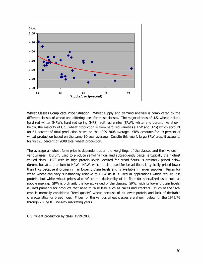
50

2.00

2.50

3.00

3.50

4.00

4.50

5.00

15 35 55 75 95S tocks/use (percent)

$/bu.

Wheat Classes Complicate Price Situation. Wheat supply and demand analysis is complicated by the different classes of wheat and differing uses for these classes. The major classes of U.S. wheat include hard red winter (HRW), hard red spring (HRS), soft red winter (SRW), white, and durum. As shown below, the majority of U.S. wheat production is from hard red varieties (HRW and HRS) which account for 64 percent of total production based on the 1999-2008 average. SRW accounts for 19 percent of wheat production based on the same 10-year average. Despite this year�s large SRW crop, it accounts for just 25 percent of 2008 total wheat production. The average all-wheat farm price is dependent upon the weightings of the classes and their values in various uses. Durum, used to produce semolina flour and subsequently pasta, is typically the highest valued class. HRS with its high protein levels, desired for bread flours, is ordinarily priced below durum, but at a premium to HRW. HRW, which is also used for bread flour, is typically priced lower than HRS because it ordinarily has lower protein levels and is available in larger supplies. Prices for white wheat can vary substantially relative to HRW as it is used in applications which require less protein, but white wheat prices also reflect the desirability of its flour for specialized uses such as noodle making. SRW is ordinarily the lowest valued of the classes. SRW, with its lower protein levels, is used primarily for products that need to raise less, such as cakes and crackers. Much of the SRW crop is normally considered �feed quality� wheat because of its lower protein and lack of desirable characteristics for bread flour. Prices for the various wheat classes are shown below for the 1975/76 through 2007/08 June-May marketing years. U.S. wheat production by class, 1999-2008

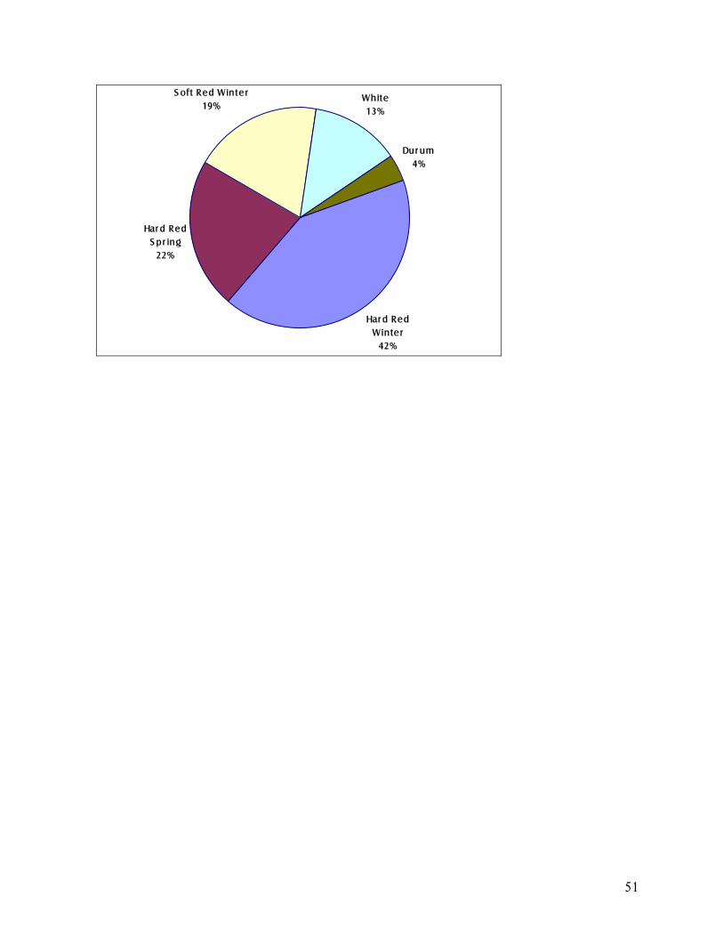
51

Har d Red S pr ing

22%

S oft Red Winter19%

White13%

Dur um4%

Har d Red Winter

42%

52

Wheat farm prices by class

2.00

3.00

4.00

5.00

6.00

7.00

8.00

9.00

10.00

2000/01 2001/02 2002/03 2003/04 2004/05 2005/06 2006/07 2007/08

$/bu.

Hard Red W inter S oft Red Winter

Durum Hard Red S pring

White

Wheat Stocks-to-use Price Models. The relationship between stocks-to-use and wheat prices has been analyzed and modeled by USDA. Westcott and Hoffman estimated a model for wheat farm prices that includes stocks-to-use using 1975/76 through 1996/97 data. As with the corn price model, the wheat model accounts for farm policy impacts from supply control and price support programs during the late 1970s and 1980s. With the United States a less dominant wheat producer and exporter as compared with corn, the model also accounts for supplies and use in the major export competitor countries of Argentina, Australia, Canada, and the European Union. Because wheat competes with corn in some feed markets, particularly during the summer months, the model also includes the summer (June-August) price of corn as a variable to explain wheat prices. Westcott and Hoffman showed that the wheat price model tracked actual prices during the 1975-76 through 1996/97 period very well as shown below. The mean absolute error for the model over the sample period was 13 cents per bushel and the mean absolute error percentage was 3.9 percent. As the 2007/08 farm price and the November WASDE 2008/09 projection indicate, current prices are well above levels explained by this model.

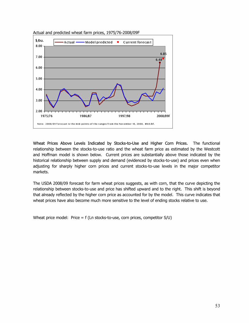
53

Actual and predicted wheat farm prices, 1975/76-2008/09F

6.48

6.85

2.00

3.00

4.00

5.00

6.00

7.00

8.00

1975/76 1986/87 1997/98 2008/09F

$/bu. A ctual Model pr edicted C ur rent for ecas t

N o t e : 2 0 0 8 / 0 9 f o r e c a s t i s t he m i d - p o i n t s o f t he r a n g e s f r o m t h e N o v e m b e r 10 , 2 0 0 8 , W A S D E .

Wheat Prices Above Levels Indicated by Stocks-to-Use and Higher Corn Prices. The functional relationship between the stocks-to-use ratio and the wheat farm price as estimated by the Westcott and Hoffman model is shown below. Current prices are substantially above those indicated by the historical relationship between supply and demand (evidenced by stocks-to-use) and prices even when adjusting for sharply higher corn prices and current stocks-to-use levels in the major competitor markets. The USDA 2008/09 forecast for farm wheat prices suggests, as with corn, that the curve depicting the relationship between stocks-to-use and price has shifted upward and to the right. This shift is beyond that already reflected by the higher corn price as accounted for by the model. This curve indicates that wheat prices have also become much more sensitive to the level of ending stocks relative to use. Wheat price model: Price = f (Ln stocks-to-use, corn prices, competitor S/U)

54

2.00

3.00

4.00

5.00

6.00

7.00

8.00

9.00

0 10 20 30 40 50 60S tocks /us e (percent)

$/bu. W heat pr ic e model Forec as t Actual

2008/092007/08

N ot e : 2 0 0 8 / 0 9 f o r e c a s t i s t h e m i d - p o i n t o f t he r a n g e f r o m t h e N ov e mb e r 10 , 2 0 0 8 , W A S D E .

Farm prices for wheat during 2002/03 through 2006/07 were relatively consistent with those predicted by the price model when the function is adjusted for lower corn prices during that period. Summer quarter corn prices for 2002 through 2006 ranged from $2.03 to $2.55 per bushel. The wheat price function is adjusted below and shown reflecting the average $2.22-per-bushel corn price for those years. Conversely, using the 2008 summer (June-August) corn price of $5.33 per bushel boosts the wheat price function, but it still falls well below the level indicated by the November WASDE 2008/09 price forecast. Wheat price model: Stocks-to-use relationship shifted

6.856.48

2.00

4.00

6.00

8.00

10.00

12.00

14.00

16.00

18.00

20.00

0 10 20 30 40 50 60S tock s /us e (per cent)

$/bu. Wheat pr ice m odel ($5.33 cor n)Wheat pr ice m odel ($2.22 cor n)For ecas tA ctual

2008/09

2007/08

N ot e : 2 0 0 7 / 0 8 a n d 2 0 0 8 / 0 9 f o r e c a s t s a r e t h e m i d - p o i n t s o f t h e r a ng e s f r o m t h e N ov e m b e r 10 , 2 0 0 8 ,

A ctual pr ices 2002/03- 2007/08

55

Wheat Cash and Futures Prices Diverge. Futures prices for soft red winter (SRW) wheat have remained high relative to those for hard red winter (HRW) wheat and corn even as cash prices show a much different situation in the market for the physical commodity.

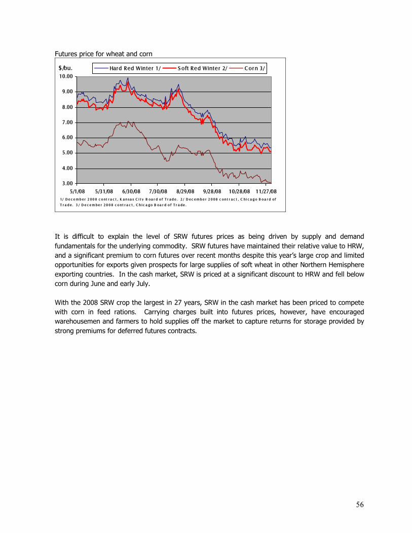
56

Futures price for wheat and corn

3.00

4.00

5.00

6.00

7.00

8.00

9.00

10.00

5/1/08 5/31/08 6/30/08 7/30/08 8/29/08 9/28/08 10/28/08 11/27/08

$/bu. Hard Red Winter 1/ S oft Red Winter 2/ C or n 3/

1/ D e c e m b e r 2 0 0 8 c o n t r a c t , K a n sa s C i t y B oa r d o f T r a d e . 2 / D e c e m b e r 2 0 0 8 c on t r a c t , C h i c a g o B o a r d o f

T r a d e . 3 / D e c e m b e r 2 0 0 8 c o n t r a c t , C h i c a g o B oa r d o f T r a d e .

It is difficult to explain the level of SRW futures prices as being driven by supply and demand fundamentals for the underlying commodity. SRW futures have maintained their relative value to HRW, and a significant premium to corn futures over recent months despite this year�s large crop and limited opportunities for exports given prospects for large supplies of soft wheat in other Northern Hemisphere exporting countries. In the cash market, SRW is priced at a significant discount to HRW and fell below corn during June and early July. With the 2008 SRW crop the largest in 27 years, SRW in the cash market has been priced to compete with corn in feed rations. Carrying charges built into futures prices, however, have encouraged warehousemen and farmers to hold supplies off the market to capture returns for storage provided by strong premiums for deferred futures contracts.

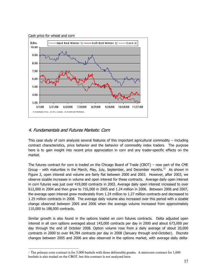
57

Cash price for wheat and corn

3.00

4.00

5.00

6.00

7.00

8.00

9.00

10.00

5/1/08 5/31/08 6/30/08 7/30/08 8/29/08 9/28/08 10/28/08 11/27/08

$/bu. Hard Red Winter 1/ S oft Red Winter 2/ C or n 3/

1/ K a ns a s C i t y . 2 / S t . L o u i s . 3 / C e n t r a l I l l i n o i s .

4. Fundamentals and Futures Markets: Corn This case study of corn analyzes several features of this important agricultural commodity � including contract characteristics, price behavior and the behavior of commodity index traders. The purpose here is to gain insight into recent price appreciation in corn and any trader-specific effects on the market. The futures contract for corn is traded on the Chicago Board of Trade (CBOT) � now part of the CME Group - with maturities in the March, May, July, September, and December months.12 As shown in Figure 2, open interest and volume are fairly flat between 2000 and 2003. However, after 2003, we observe sizable increases in volume and open interest for these contracts. Average daily open interest in corn futures was just over 419,000 contracts in 2003. Average daily open interest increased to over 612,000 in 2004 and then grew to 716,000 in 2005 and 1.24 million in 2006. Between 2006 and 2007, the average open interest grew moderately from 1.24 million to 1.27 million contracts and decreased to 1.25 million contracts in 2008. The average daily volume also increased over this period with a sizable change observed between 2005 and 2006 when the average volume increased from approximately 110,000 to 188,000 contracts. Similar growth is also found in the options traded on corn futures contracts. Delta adjusted open interest in all corn options averaged about 143,000 contracts per day in 2000 and about 673,000 per day through the end of October 2008. Option volume rose from a daily average of about 20,000 contracts in 2000 to over 84,784 contracts per day in 2008 (January through end-October). Discrete changes between 2005 and 2006 are also observed in the options market, with average daily delta-

12 The primary corn contract is for 5,000 bushels with three deliverable grades. A mini-corn contract for 1,000 bushels is also traded on the CBOT, but this contract is not analyzed here.

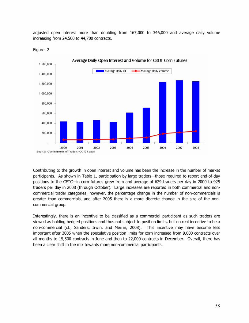
58

adjusted open interest more than doubling from 167,000 to 346,000 and average daily volume increasing from 24,500 to 44,700 contracts. Figure 2

Average Daily Open Interest and Volume for CBOT Corn Futures

-

200,000

400,000

600,000

800,000

1,000,000

1,200,000

1,400,000

1,600,000

2000 2001 2002 2003 2004 2005 2006 2007 2008

Average Daily OI Average Daily Volume

S ource: C ommitments of T raders (C OT ) R eport

Contributing to the growth in open interest and volume has been the increase in the number of market participants. As shown in Table 1, participation by large traders�those required to report end-of-day positions to the CFTC�in corn futures grew from and average of 629 traders per day in 2000 to 925 traders per day in 2008 (through October). Large increases are reported in both commercial and non-commercial trader categories; however, the percentage change in the number of non-commercials is greater than commercials, and after 2005 there is a more discrete change in the size of the non-commercial group. Interestingly, there is an incentive to be classified as a commercial participant as such traders are viewed as holding hedged positions and thus not subject to position limits, but no real incentive to be a non-commercial (cf., Sanders, Irwin, and Merrin, 2008). This incentive may have become less important after 2005 when the speculative position limits for corn increased from 9,000 contracts over all months to 15,500 contracts in June and then to 22,000 contracts in December. Overall, there has been a clear shift in the mix towards more non-commercial participants.

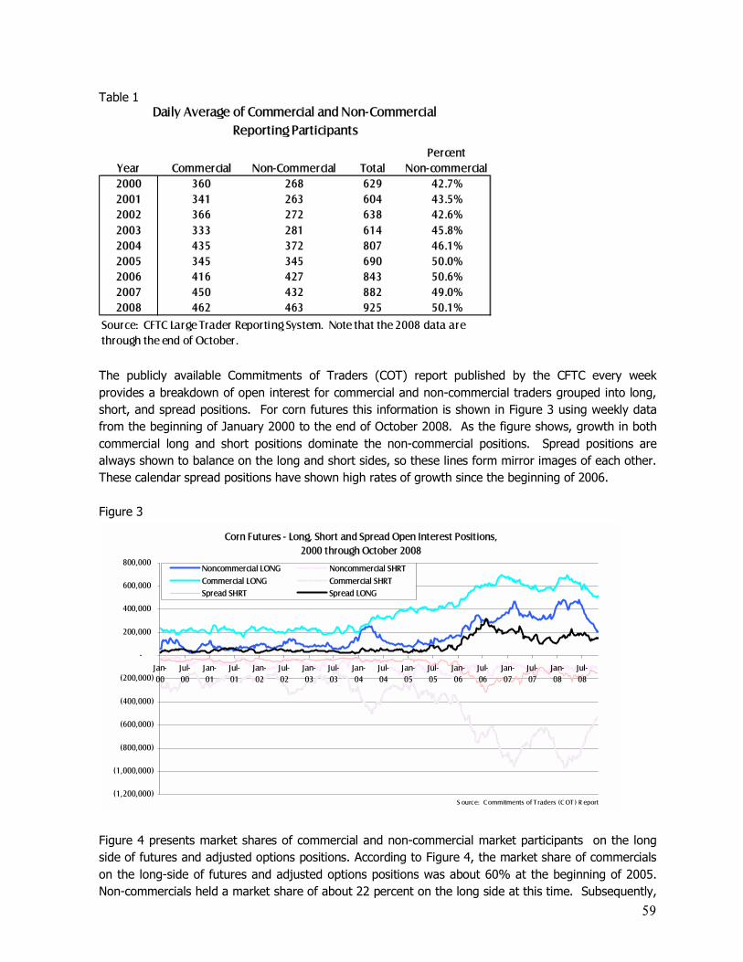
59

Table 1

Year Commercial Non-Commercial TotalPercent

Non-commercial2000 360 268 629 42.7%2001 341 263 604 43.5%2002 366 272 638 42.6%2003 333 281 614 45.8%2004 435 372 807 46.1%2005 345 345 690 50.0%2006 416 427 843 50.6%2007 450 432 882 49.0%2008 462 463 925 50.1%

Source: CFTC Large Trader Reporting System. Note that the 2008 data are through the end of October.

Daily Average of Commercial and Non-CommercialReporting Participants

The publicly available Commitments of Traders (COT) report published by the CFTC every week provides a breakdown of open interest for commercial and non-commercial traders grouped into long, short, and spread positions. For corn futures this information is shown in Figure 3 using weekly data from the beginning of January 2000 to the end of October 2008. As the figure shows, growth in both commercial long and short positions dominate the non-commercial positions. Spread positions are always shown to balance on the long and short sides, so these lines form mirror images of each other. These calendar spread positions have shown high rates of growth since the beginning of 2006. Figure 3

Corn Futures - Long, Short and Spread Open Interest Positions, 2000 through October 2008

(1,200,000)

(1,000,000)

(800,000)

(600,000)

(400,000)

(200,000)

-

200,000

400,000

600,000

800,000

Jan-00

Jul-00

Jan-01

Jul-01

Jan-02

Jul-02

Jan-03

Jul-03

Jan-04

Jul-04

Jan-05

Jul-05

Jan-06

Jul-06

Jan-07

Jul-07

Jan-08

Jul-08

Noncommercial LONG Noncommercial SHRT

Commercial LONG Commercial SHRT

Spread SHRT Spread LONG

S ource: C ommitments of T raders (C OT ) R eport

Figure 4 presents market shares of commercial and non-commercial market participants on the long side of futures and adjusted options positions. According to Figure 4, the market share of commercials on the long-side of futures and adjusted options positions was about 60% at the beginning of 2005. Non-commercials held a market share of about 22 percent on the long side at this time. Subsequently,

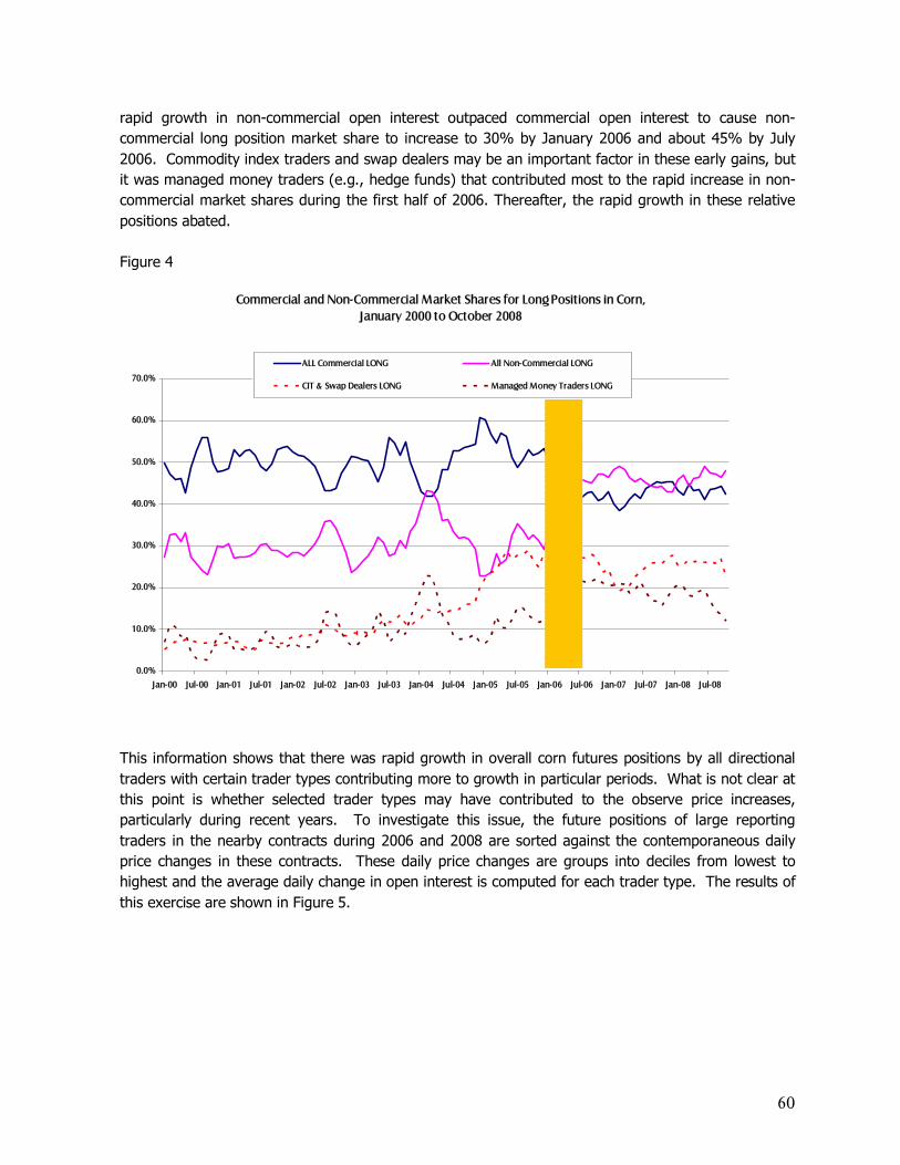
60

rapid growth in non-commercial open interest outpaced commercial open interest to cause non-commercial long position market share to increase to 30% by January 2006 and about 45% by July 2006. Commodity index traders and swap dealers may be an important factor in these early gains, but it was managed money traders (e.g., hedge funds) that contributed most to the rapid increase in non-commercial market shares during the first half of 2006. Thereafter, the rapid growth in these relative positions abated. Figure 4

Commercial and Non-Commercial Market Shares for Long Positions in Corn, January 2000 to October 2008

0.0%

10.0%

20.0%

30.0%

40.0%

50.0%

60.0%

70.0%

Jan-00 Jul-00 Jan-01 Jul-01 Jan-02 Jul-02 Jan-03 Jul-03 Jan-04 Jul-04 Jan-05 Jul-05 Jan-06 Jul-06 Jan-07 Jul-07 Jan-08 Jul-08

ALL Commercial LONG All Non-Commercial LONG

CIT & Swap Dealers LONG Managed Money Traders LONG

This information shows that there was rapid growth in overall corn futures positions by all directional traders with certain trader types contributing more to growth in particular periods. What is not clear at this point is whether selected trader types may have contributed to the observe price increases, particularly during recent years. To investigate this issue, the future positions of large reporting traders in the nearby contracts during 2006 and 2008 are sorted against the contemporaneous daily price changes in these contracts. These daily price changes are groups into deciles from lowest to highest and the average daily change in open interest is computed for each trader type. The results of this exercise are shown in Figure 5.

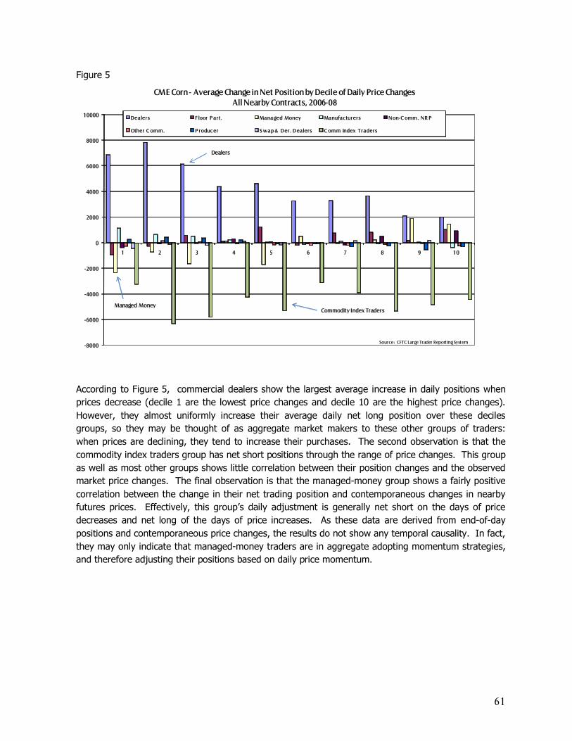
61

Figure 5

-8000

-6000

-4000

-2000

0

2000

4000

6000

8000

10000

1 2 3 4 5 6 7 8 9 10

CME Corn - Average Change in Net Position by Decile of Daily Price ChangesAll Nearby Contracts, 2006-08

Dealers F loor P art. Managed Money Manufacturers Non-C omm. NR P

Other C omm. P roduc er S wap & Der. Dealers C omm Index T raders

Source: CFTC Large Trader Reporting System

Commodity Index Traders

Dealers

Managed Money

According to Figure 5, commercial dealers show the largest average increase in daily positions when prices decrease (decile 1 are the lowest price changes and decile 10 are the highest price changes). However, they almost uniformly increase their average daily net long position over these deciles groups, so they may be thought of as aggregate market makers to these other groups of traders: when prices are declining, they tend to increase their purchases. The second observation is that the commodity index traders group has net short positions through the range of price changes. This group as well as most other groups shows little correlation between their position changes and the observed market price changes. The final observation is that the managed-money group shows a fairly positive correlation between the change in their net trading position and contemporaneous changes in nearby futures prices. Effectively, this group�s daily adjustment is generally net short on the days of price decreases and net long of the days of price increases. As these data are derived from end-of-day positions and contemporaneous price changes, the results do not show any temporal causality. In fact, they may only indicate that managed-money traders are in aggregate adopting momentum strategies, and therefore adjusting their positions based on daily price momentum.

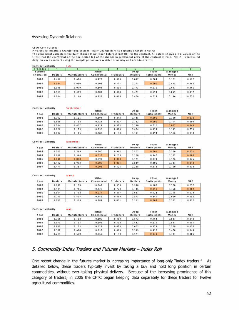
62

Assessing Dynamic Relations C B O T C or n F u t u r esP - V a lu es fo r B iv a r ia t e G r a n g e r R e g r es s ion s - D a i ly C h a ng e in P r ic e E x p la in s C h a ng e in N e t OI

C on t r a c t Ma t u r it y J u lyT r dc od es 1 2 3 4 5 6 7 8F ut u r e s

E x p i r a t ion D e a le r s Ma n u fa c t u r e r sOt h er

C om m e r c ia l P r od u c er sS w a p

D e a ler sF lo or

P a r t ic ipa n t sMa na g ed

Mon ey N R P

2 0 0 3 0 .436 0 .674 0 .477 0 .469 0 .097 0 .284 0 .121 0 .622

2 0 0 4 0 .044 0 .630 0 .908 0 .371 0 .273 0 .000 0 .835 0 .983

2 0 0 5 0 .095 0 .079 0 .891 0 .606 0 .173 0 .075 0 .947 0 .495

2 0 0 6 0 .911 0 .489 0 .203 0 .404 0 .471 0 .693 0 .855 0 .417

2 0 0 7 0 .064 0 .116 0 .959 0 .065 0 .406 0 .725 0 .186 0 .772

C on t r a c t Ma t u r it y S e p t em b er

Y e a r D e a le r s Ma n u fa c t u r e r sOt h er

C om m e r c ia l P r od u c er sS w a p

D e a ler sF lo or

P a r t ic ipa n t sMa na g ed

Mon ey N R P

2 0 0 3 0 .762 0 .525 0 .891 0 .243 0 .445 0 .005 0 .760 0 .070

2 0 0 4 0 .606 0 .158 0 .724 0 .837 0 .732 0 .000 0 .114 0 .609

2 0 0 5 0 .704 0 .407 0 .824 0 .572 0 .330 0 .710 0 .007 0 .046

2 0 0 6 0 .126 0 .175 0 .290 0 .085 0 .424 0 .559 0 .155 0 .756

2 0 0 7 0 .092 0 .115 0 .288 0 .140 0 .191 0 .394 0 .516 0 .918

C on t r a c t Ma t u r it y D e c em be r

Y e a r D e a le r s Ma n u fa c t u r e r sOt h er

C om m e r c ia l P r od u c er sS w a p

D e a ler sF lo or

P a r t ic ipa n t sMa na g ed

Mon ey N R P

2 0 0 3 0 .520 0 .519 0 .260 0 .912 0 .507 0 .001 0 .320 0 .031

2 0 0 4 0 .608 0 .548 0 .037 0 .258 0 .220 0 .547 0 .107 0 .000

2 0 0 5 0 .048 0 .000 0 .093 0 .000 0 .171 0 .073 0 .176 0 .825

2 0 0 6 0 .412 0 .992 0 .000 0 .001 0 .849 0 .205 0 .387 0 .013

2 0 0 7 0 .471 0 .387 0 .008 0 .325 0 .238 0 .318 0 .150 0 .438

C on t r a c t Ma t u r it y Ma r c h

Y e a r D e a le r s Ma n u fa c t u r e r sOt h er

C om m e r c ia l P r od u c er sS w a p

D e a ler sF lo or

P a r t ic ipa n t sMa na g ed

Mon ey N R P

2 0 0 3 0 .149 0 .139 0 .265 0 .359 0 .998 0 .100 0 .528 0 .252

2 0 0 4 0 .544 0 .716 0 .820 0 .728 0 .436 0 .050 0 .358 0 .002

2 0 0 5 0 .864 0 .758 0 .037 0 .497 0 .633 0 .124 0 .718 0 .678

2 0 0 6 0 .730 0 .495 0 .442 0 .469 0 .593 0 .841 0 .920 0 .153

2 0 0 7 0 .067 0 .369 0 .384 0 .051 0 .313 0 .009 0 .307 0 .852

C on t r a c t Ma t u r it y Ma y

Y e a r D e a le r s Ma n u fa c t u r e r sOt h er

C om m e r c ia l P r od u c er sS w a p

D e a ler sF lo or

P a r t ic ipa n t sMa na g ed

Mon ey N R P

2 0 0 3 0 .766 0 .138 0 .300 0 .389 0 .572 0 .164 0 .887 0 .243

2 0 0 4 0 .570 0 .133 0 .295 0 .534 0 .442 0 .275 0 .841 0 .051

2 0 0 5 0 .800 0 .123 0 .629 0 .476 0 .605 0 .373 0 .529 0 .150

2 0 0 6 0 .508 0 .690 0 .237 0 .485 0 .559 0 .450 0 .478 0 .349

2 0 0 7 0 .211 0 .670 0 .065 0 .144 0 .574 0 .039 0 .491 0 .386

T h e de pe n de n t v a r ia b le is t h e d a i ly c h a n ge in n e t O pe n I n t e r e s t ( n et O I ) fo r t h e c on t r a c t . A l l v a lu e s s h ow n a r e p - v a lu es of t h et - t e s t t ha t t h e co ef f ic ie n t o f t h e o ne - p er io d la g of t h e ch a n ge in s e t t le m en t p r ic e of t he c on t r a ct i s zer o . N e t O I is m ea s u r e dd a i ly fo r ea c h c on t r a c t us in g t h e s a m p le p e r iod ov e r w h ic h i t is n e a r by a n d n ex t - t o - n ea r b y .

5. Commodity Index Traders and Futures Markets � Index Roll One recent change in the futures market is increasing importance of long-only �index traders.� As detailed below, these traders typically invest by taking a buy and hold long position in certain commodities, without ever taking physical delivery. Because of the increasing prominence of this category of traders, in 2006 the CFTC began keeping data separately for these traders for twelve agricultural commodities.

63

Based on these data, several aspects of the extent of index fund activity for the three most widely-traded agricultural commodities (soy beans, corn and wheat) are apparent. First, index traders on average represent about than 30% of total futures open interest in soy beans and corn, and between 40 and 50% for wheat. Figure 1 portrays the percentage of total futures open interest in these commodities accounted for by index funds over the past 32 months.13 For all three commodities, the percentage has remained fairly stable over this period.14 For example, for soy beans, CIT represent between 28 and 34% of the open interest during the sample period. Second, index funds are disproportionately invested in a single-maturity contract, often the nearest-to-maturity (the nearby). For example, as of February 1, 2008, roughly half of index fund future positions in soy beans were invested in the March, 2008 contract, so that index traders represented nearly 43% of all futures open interest in that contract.

C IT S har es of Futur es Open Inter es t

0

0.1

0.2

0.3

0.4

0.5

0.6

12/14/2005

3/24/2006

7/2/2006 10/10/2006

1/18/2007

4/28/2007

8/6/2007 11/14/2007

2/22/2008

6/1/2008 9/9/2008

w heat

corn

s oy

The fact that index traders are primarily invested in the nearby means that as that contract nears maturity, an index trader needs to move his investment into a contract with a later maturity. The movement of a trader�s investment into a contract with a later maturity is often referred to as rolling the position forward. Figure 2 illustrates a typical pattern of rolling for index traders as a whole. As shown there, as of July 15, 2006, index traders held a long position of about 150,000 futures contracts in the nearby wheat contract (the September, 2006 contract). Over the next twenty trading days, index traders reduced their holdings in that contract to less than 30,000 thousand contracts, while simultaneously increasing their positions in the December, 2006 contract by a similar amount. Five trading days are characterized by particularly large rolling; August 7 � 11, during which index traders reduced their positions by about 15,000 contracts per day. These are the five trading days during which the largest index fund, the Goldman Sachs Commodity Index (GSCI), rolls its position. These 5 days are often referred to as the Goldman Roll period.

13 The percentage shown there is the share of total futures open interest accounted for by CITs, as of 49 days prior to contract expiration (i.e., before the CIT positions are unwound). 14 Because index funds primarily trade in futures, not options, index funds shares of all futures and options in these products is smaller, and has trended downward over the sample period.

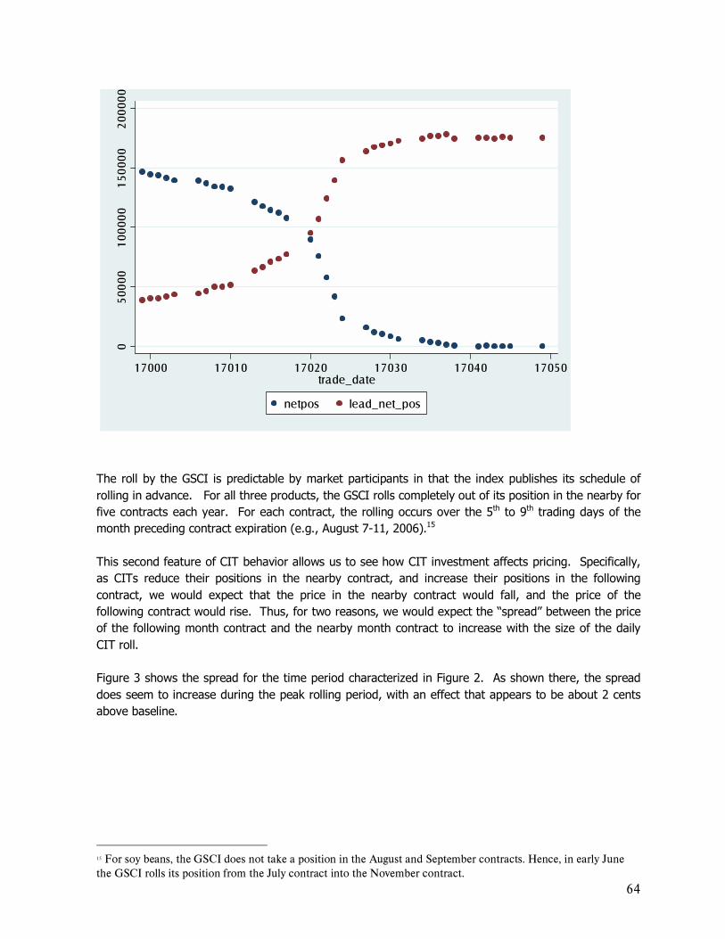
64

05

0000

100

000

150

000

200

000

17000 17010 17020 17030 17040 17050trade_date

netpos lead_net_pos

The roll by the GSCI is predictable by market participants in that the index publishes its schedule of rolling in advance. For all three products, the GSCI rolls completely out of its position in the nearby for five contracts each year. For each contract, the rolling occurs over the 5th to 9th trading days of the month preceding contract expiration (e.g., August 7-11, 2006).15 This second feature of CIT behavior allows us to see how CIT investment affects pricing. Specifically, as CITs reduce their positions in the nearby contract, and increase their positions in the following contract, we would expect that the price in the nearby contract would fall, and the price of the following contract would rise. Thus, for two reasons, we would expect the �spread� between the price of the following month contract and the nearby month contract to increase with the size of the daily CIT roll. Figure 3 shows the spread for the time period characterized in Figure 2. As shown there, the spread does seem to increase during the peak rolling period, with an effect that appears to be about 2 cents above baseline.

15 For soy beans, the GSCI does not take a position in the August and September contracts. Hence, in early June the GSCI rolls its position from the July contract into the November contract.

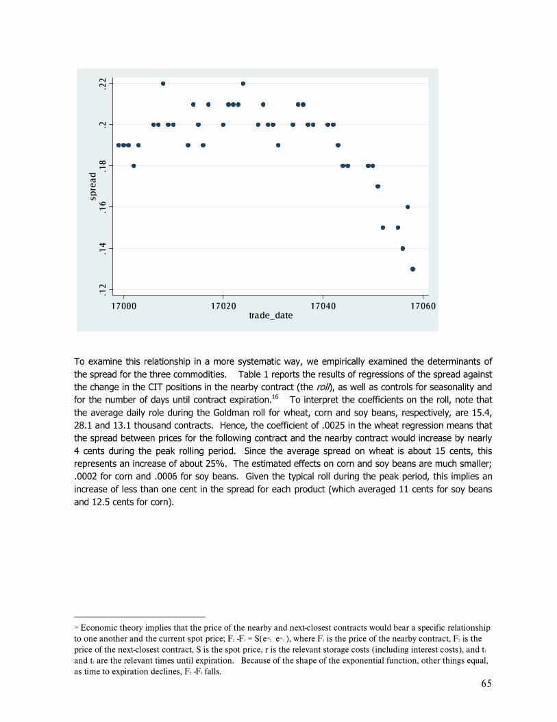
65

.12

.14

.16

.18

.2.2

2sp

rea

d

17000 17020 17040 17060trade_date

To examine this relationship in a more systematic way, we empirically examined the determinants of the spread for the three commodities. Table 1 reports the results of regressions of the spread against the change in the CIT positions in the nearby contract (the roll), as well as controls for seasonality and for the number of days until contract expiration.16 To interpret the coefficients on the roll, note that the average daily role during the Goldman roll for wheat, corn and soy beans, respectively, are 15.4, 28.1 and 13.1 thousand contracts. Hence, the coefficient of .0025 in the wheat regression means that the spread between prices for the following contract and the nearby contract would increase by nearly 4 cents during the peak rolling period. Since the average spread on wheat is about 15 cents, this represents an increase of about 25%. The estimated effects on corn and soy beans are much smaller; .0002 for corn and .0006 for soy beans. Given the typical roll during the peak period, this implies an increase of less than one cent in the spread for each product (which averaged 11 cents for soy beans and 12.5 cents for corn).

16 Economic theory implies that the price of the nearby and next-closest contracts would bear a specific relationship to one another and the current spot price; F2 -F1 = S(e-rt

2 - e-rt

1 ), where F1 is the price of the nearby contract, F2 is the price of the next-closest contract, S is the spot price, r is the relevant storage costs (including interest costs), and t1 and t2 are the relevant times until expiration. Because of the shape of the exponential function, other things equal, as time to expiration declines, F2 -F1 falls.

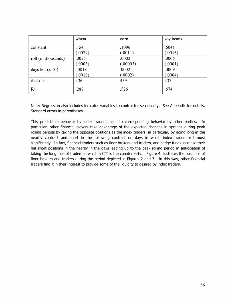
66

wheat corn soy beans

constant .154 (.0079)

.1096 (.0011)

.6041 (.0016)

roll (in thousands) .0025 (.0003)

.0002 (.00003)

.0006 (.0001)

days left (x 10) -.0018 (.0018)

-0002 (.0002)

.0009 (.0004)

# of obs. 436 439 437

R2 .288 .526 .674

Note: Regression also includes indicator variables to control for seasonality. See Appendix for details. Standard errors in parentheses This predictable behavior by index traders leads to corresponding behavior by other parties. In particular, other financial players take advantage of the expected changes in spreads during peak rolling periods by taking the opposite positions as the index traders; in particular, by going long in the nearby contract and short in the following contract on days in which index traders roll most significantly. In fact, financial traders such as floor brokers and traders, and hedge funds increase their net short positions in the nearby in the days leading up to the peak rolling period in anticipation of taking the long side of traders in which a CIT is the counterparty. Figure 4 illustrates the positions of floor brokers and traders during the period depicted in Figures 2 and 3. In this way, other financial traders find it in their interest to provide some of the liquidity to desired by index traders.

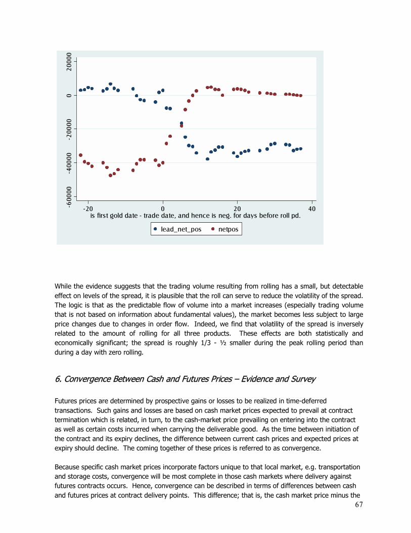
67

-600

00-4

0000

-200

000

200

00

- 20 0 20 40is first gold date - trade date, and hence is neg. for days before roll pd.

lead_net_pos netpos

While the evidence suggests that the trading volume resulting from rolling has a small, but detectable effect on levels of the spread, it is plausible that the roll can serve to reduce the volatility of the spread. The logic is that as the predictable flow of volume into a market increases (especially trading volume that is not based on information about fundamental values), the market becomes less subject to large price changes due to changes in order flow. Indeed, we find that volatility of the spread is inversely related to the amount of rolling for all three products. These effects are both statistically and economically significant; the spread is roughly 1/3 - ½ smaller during the peak rolling period than during a day with zero rolling.

6. Convergence Between Cash and Futures Prices � Evidence and Survey Futures prices are determined by prospective gains or losses to be realized in time-deferred transactions. Such gains and losses are based on cash market prices expected to prevail at contract termination which is related, in turn, to the cash-market price prevailing on entering into the contract as well as certain costs incurred when carrying the deliverable good. As the time between initiation of the contract and its expiry declines, the difference between current cash prices and expected prices at expiry should decline. The coming together of these prices is referred to as convergence. Because specific cash market prices incorporate factors unique to that local market, e.g. transportation and storage costs, convergence will be most complete in those cash markets where delivery against futures contracts occurs. Hence, convergence can be described in terms of differences between cash and futures prices at contract delivery points. This difference; that is, the cash market price minus the

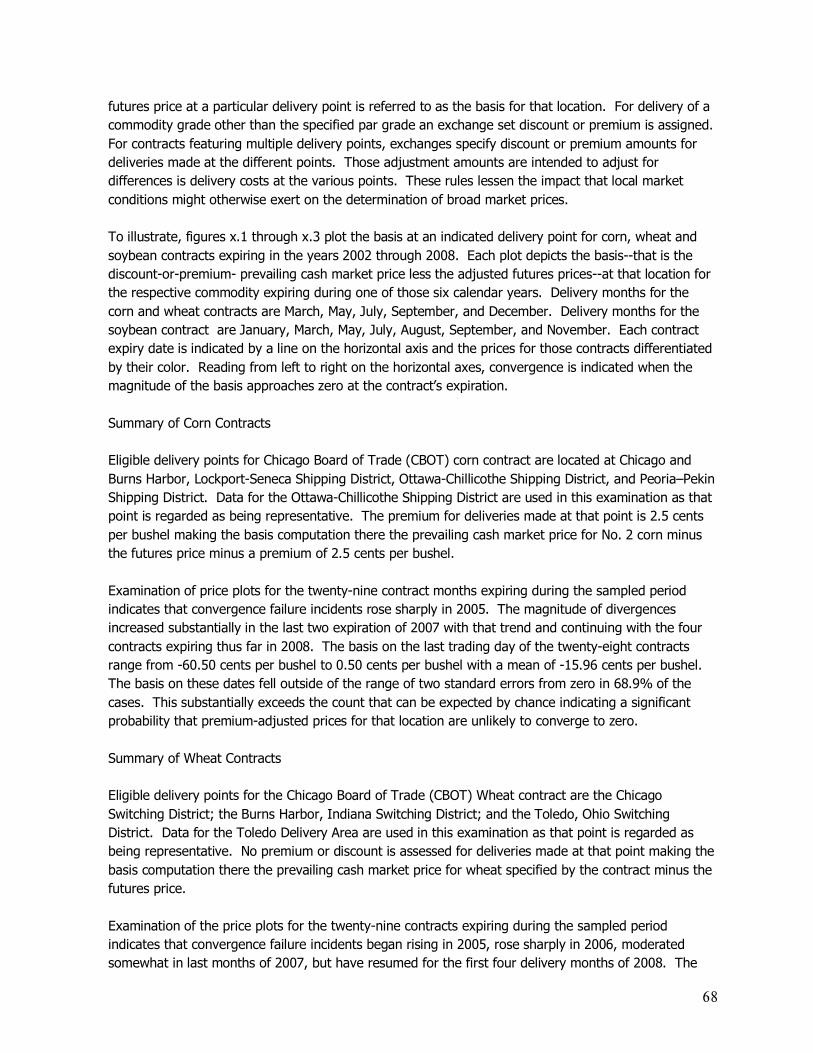
68

futures price at a particular delivery point is referred to as the basis for that location. For delivery of a commodity grade other than the specified par grade an exchange set discount or premium is assigned. For contracts featuring multiple delivery points, exchanges specify discount or premium amounts for deliveries made at the different points. Those adjustment amounts are intended to adjust for differences is delivery costs at the various points. These rules lessen the impact that local market conditions might otherwise exert on the determination of broad market prices. To illustrate, figures x.1 through x.3 plot the basis at an indicated delivery point for corn, wheat and soybean contracts expiring in the years 2002 through 2008. Each plot depicts the basis--that is the discount-or-premium- prevailing cash market price less the adjusted futures prices--at that location for the respective commodity expiring during one of those six calendar years. Delivery months for the corn and wheat contracts are March, May, July, September, and December. Delivery months for the soybean contract are January, March, May, July, August, September, and November. Each contract expiry date is indicated by a line on the horizontal axis and the prices for those contracts differentiated by their color. Reading from left to right on the horizontal axes, convergence is indicated when the magnitude of the basis approaches zero at the contract�s expiration. Summary of Corn Contracts Eligible delivery points for Chicago Board of Trade (CBOT) corn contract are located at Chicago and Burns Harbor, Lockport-Seneca Shipping District, Ottawa-Chillicothe Shipping District, and Peoria�Pekin Shipping District. Data for the Ottawa-Chillicothe Shipping District are used in this examination as that point is regarded as being representative. The premium for deliveries made at that point is 2.5 cents per bushel making the basis computation there the prevailing cash market price for No. 2 corn minus the futures price minus a premium of 2.5 cents per bushel. Examination of price plots for the twenty-nine contract months expiring during the sampled period indicates that convergence failure incidents rose sharply in 2005. The magnitude of divergences increased substantially in the last two expiration of 2007 with that trend and continuing with the four contracts expiring thus far in 2008. The basis on the last trading day of the twenty-eight contracts range from -60.50 cents per bushel to 0.50 cents per bushel with a mean of -15.96 cents per bushel. The basis on these dates fell outside of the range of two standard errors from zero in 68.9% of the cases. This substantially exceeds the count that can be expected by chance indicating a significant probability that premium-adjusted prices for that location are unlikely to converge to zero. Summary of Wheat Contracts Eligible delivery points for the Chicago Board of Trade (CBOT) Wheat contract are the Chicago Switching District; the Burns Harbor, Indiana Switching District; and the Toledo, Ohio Switching District. Data for the Toledo Delivery Area are used in this examination as that point is regarded as being representative. No premium or discount is assessed for deliveries made at that point making the basis computation there the prevailing cash market price for wheat specified by the contract minus the futures price. Examination of the price plots for the twenty-nine contracts expiring during the sampled period indicates that convergence failure incidents began rising in 2005, rose sharply in 2006, moderated somewhat in last months of 2007, but have resumed for the first four delivery months of 2008. The

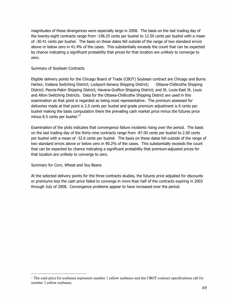
69

magnitudes of these divergences were especially large in 2008. The basis on the last trading day of the twenty-eight contracts range from -198.25 cents per bushel to 12.50 cents per bushel with a mean of -30.41 cents per bushel. The basis on these dates fell outside of the range of two standard errors above or below zero in 41.4% of the cases. This substantially exceeds the count that can be expected by chance indicating a significant probability that prices for that location are unlikely to converge to zero. Summary of Soybean Contracts Eligible delivery points for the Chicago Board of Trade (CBOT) Soybean contract are Chicago and Burns Harbor, Indiana Switching District; Lockport-Seneca Shipping District; Ottawa-Chillicothe Shipping District; Peoria-Pekin Shipping District; Havana-Grafton Shipping District; and St. Louis-East St. Louis and Alton Switching Districts. Data for the Ottawa-Chillicothe Shipping District are used in this examination as that point is regarded as being most representative. The premium assessed for deliveries made at that point is 2.5 cents per bushel and grade premium adjustment is 6 cents per bushel making the basis computation there the prevailing cash market price minus the futures price minus 8.5 cents per bushel.17 Examination of the plots indicates that convergence failure incidents rising over the period. The basis on the last trading day of the thirty-nine contracts range from -87.00 cents per bushel to 2.00 cents per bushel with a mean of -32.6 cents per bushel. The basis on these dates fell outside of the range of two standard errors above or below zero in 90.2% of the cases. This substantially exceeds the count that can be expected by chance indicating a significant probability that premium-adjusted prices for that location are unlikely to converge to zero. Summary for Corn, Wheat and Soy Beans At the selected delivery points for the three contracts studies, the futures price adjusted for discounts or premiums less the cash price failed to converge in more than half of the contracts expiring in 2003 through July of 2008. Convergence problems appear to have increased over the period.

17 The cash price for soybeans represents number 1 yellow soybeans and the CBOT contract specifications call for number 2 yellow soybeans.

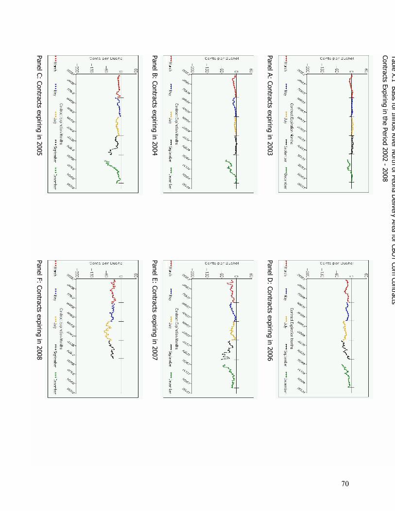
70

Panel C: Contracts expiring in 2005

Panel B: Contracts expiring in 2004

Panel A: Contracts expiring in 2003

Panel F: Contracts expiring in 2008

Panel E: Contracts expiring in 2007

Panel D

: Contracts expiring in 2006

Table X.1 Basis for Illinois River North of Peoria D

elivery Area for CBOT Corn Contracts

Contracts Expiring in the Period 2002 - 2008

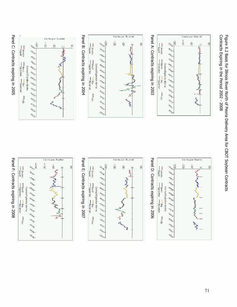
71

`

Panel C: Contracts expiring in 2005

Panel B: Contracts expiring in 2004

Panel A: Contracts expiring in 2003

Panel F: Contracts expiring in 2008

Panel E: Contracts expiring in 2007

Panel D

: Contracts expiring in 2006

Figure X.2 Basis for Illinois River North of Peoria D

elivery Area for CBOT Soybean Contracts

Contracts Expiring in the Period 2002 - 2008

72

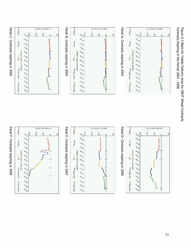
73

Panel C: Contracts expiring in 2005

Panel B: Contracts expiring in 2004

Panel A: Contracts expiring in 2003

Panel F: Contracts expiring in 2008

Panel E: Contracts expiring in 2007

Panel D

: Contracts expiring in 2006

Figure X.3 Basis for Toledo Delivery Area for CBO

T Wheat Contracts

Contracts Expiring in the Period 2002 - 2008

74

Literature Review for Research on Convergence An important aspect of a well-functioning futures contract is that contract terms reflect the realities of commercial trade. Peck and Williams (1991) find that deliveries against CBOT grain futures contracts despite their being a small proportion of contracts open interest, play an important role in that regard. That study, motivated by the deterioration of basis convergence during the 1960s through the 1980s finds increased deliveries on corn, wheat and soybean contracts as a percentage of delivery stocks. This is interpreted as evidence that deliverable stocks relative to contract outstanding at expiration were too low. They conclude that the cash trade was increasingly routed through ports located in the Gulf and the Northwest lessening the importance of the Chicago cash market. The study suggested the need to re-evaluate the delivery provisions for grain. Subsequently, the earlier delivery procedures were replaced with use of shipping certificates at locations along the Illinois Waterway system. Initially these changes, enacted starting in the 2000, dampened convergence concerns. Recently problems such as those depicted in the previous section have re-emerged. On May 11, 2005 the CFTC announced increased federal speculative position limits (CFTC Regulation 150.2) effective June 10 of that year for contracts on corn, wheat, soybean, soybean oil, soybean meal, and oats. Shortly thereafter, the CBOT announced that it would increase the levels for single-month and all-month speculative position limits. The increases came in two steps. On June 10, 2005 the levels were raised by 50% of the allowable increase in federally approved levels. Six months later, on December 10, 2005, CBOT brought its position limits fully up to the federally approved levels. Those increases prompted complaints that the added speculative activity led to increased futures prices, greater volatility, and were contributing to weak and erratic basis levels. In response, the CBOT commissioned a study of convergence for corn, soybeans, and wheat. The principal researchers in that project, Scott Irwin, Phillip Garcia, and Darrell Good focus on performance before and after the 2005 revisions to CBOT Regulation 425.01. Irwin et al adopt the �zone of convergence approach� suggested by Hiranaiova and Tomek (2002), to judge convergence performance. This approach accepts that certain contract features and costs that appropriately affect prices will preclude basis convergence to zero. This implies that convergence to zero is not a realistic performance standard. Setting aside problems related to hurricane Katrina in September 2005, convergence for the corn market failed to be within an appropriate zone starting in March, May, and July 2006 at Illinois River Locations and March, July, and September 2006 in Chicago.18 The corn basis has shown weakness since 2006 but not overall failure of convergence. Convergence problems in the soybean market began in January 2006 and continue until March 2006 except for the St. Louis market. Lack of convergence at the Illinois River existed in May, July, August and to some degree in September 2006. Similar to corn, the soybean basis is weak but a failure of convergence is not absolute. Wheat is the much more serious, with convergence failure beginning in July 2005 and persisting through September 2006. The degree of non-convergence is well outside an acceptable zone, reaching 90 cents in September 2006 contract at the Toledo location. The factors outlined by Irwin et al (2007) that relate to basis problems since 2005 include (i) sharply higher barge rates, (ii) high futures valuations, and (iii) a large carry in futures markets that influence

18 Illinois River Locations are exchange recognized delivery locations spanning from Chicago to Pekin.

75

load out decisions. Wheat is found to be a problem but basis problems with the CBOT wheat contract are not new, Gray and Peck (1981) reviewed concerns about delivery that stretch all the way back to 1920s. The fundamental problems with wheat are argued to be cash market changes in production patterns, transportation, and trade flows that have increasingly narrowed deliverable stocks. CBOT is supposed to be a soft red wheat contract but it has come to reflect world conditions for a generic wheat making that contract�s price less likely to converge with the cash price at a specific locale. Wheat continued to have convergence problems in March, May, and July 2007 with improvement in September and November 2007. Basis performance in wheat was again poor in March 2008. Soybeans problems worsened in 2007 with poor performance in March and May; worsening performance in July, August, and September; followed by improvement in November. January and March 2008 continued the poor convergence for soybeans. In general corn has show better convergence than soybeans and wheat but has still had some problems of its own in September 2007 and March 2008.

The most recent update by Irwin et al (2008b) analyzes the convergence of cash and futures. through the May 2008 contract. Wheat convergence was dismal in May 2008 along with corn, and the best convergence was seen in the soybean May 2008 contract although it was still weak. The most widely touted proposed solutions for wheat, corn, and soybean convergence weakness include (i) Make ownership of delivery instruments less attractive. The assumption is that forcing longs out before delivery will drive down the contract price and promote convergence. Two approaches have been mentioned: specifying expirations for the shipping certificates used in deliveries on futures contracts thereby forcing load out of deliverable supplies or increase storage charges applied to deliverable supplies (ii) Require that contracts cash settle, thereby forcing convergence to the cash index. (iii) Limiting hedge exemptions to manage the influence of long-only index funds. This approach assumes that speculators have induced an artificial prices increase and by limiting their positions, prices will fall toward their fundamental values. (iv) Expanding delivery capacity in order to facilitate arbitrage of cash and futures markets, which in turn theoretically promotes convergence.

C. Select Other Commodities There is a number of important commodities that do not trade in futures markets. A comparison of the behavior of spot prices between commodities that do have futures markets and those that do not offers a way to help analyze the impact of commodity index traders on commodity prices. Specifically, there are two conjectures about the relationship between index funds and commodity prices. The first conjecture is that index trading influences spot prices. The second conjecture is that the appreciation of commodity spot prices is a wide-spread phenomenon of the recent years, which is observed even in commodity markets with no futures markets. A study presented in the Appendix finds evidence in support of the second conjecture - the appreciation of commodity spot prices is a wide-spread phenomenon. The study is based on the analysis of growth rates of commodities that do and do not have futures markets.

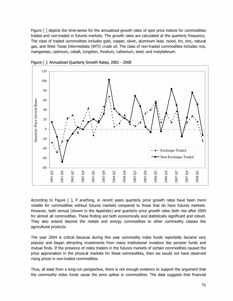
76

Figure [ ] depicts the time-series for the annualized growth rates of spot price indices for commodities traded and non-traded in futures markets. The growth rates are calculated at the quarterly frequency. The class of traded commodities includes gold, copper, silver, aluminum lead, nickel, tin, zinc, natural gas, and West Texas Intermediate (WTI) crude oil. The class of non-traded commodities includes rice, manganese, cadmium, cobalt, tungsten, rhodium, ruthenium, steel, and molybdenum. Figure [ ]: Annualized Quarterly Growth Rates, 2001 - 2008

- 80

- 60

- 40

- 20

0

20

40

60

80

100

120

200

1 Q

2

200

1 Q

4

200

2 Q

2

200

2 Q

4

200

3 Q

2

200

3 Q

4

200

4 Q

2

200

4 Q

4

200

5 Q

2

200

5 Q

4

200

6 Q

2

200

6 Q

4

200

7 Q

2

200

7 Q

4

200

8 Q

2

Exchange Traded

Non-Exchange Traded

Qua

rter

ly P

rice

Gro

wth

Rat

es

According to Figure [ ], if anything, in recent years quarterly price growth rates have been more volatile for commodities without futures markets compared to those that do have futures markets. However, both annual (shown in the Appendix) and quarterly price growth rates both rise after 2004 for almost all commodities. These finding are both economically and statistically significant and robust. They also extend beyond the metals and energy commodities to other commodity classes like agricultural products. The year 2004 is critical because during this year commodity index funds reportedly became very popular and began attracting investments from many institutional investors like pension funds and mutual finds. If the presence of index traders in the futures markets of certain commodities caused the price appreciation in the physical markets for these commodities, then we would not have observed rising prices in non-traded commodities. Thus, at least from a long-run perspective, there is not enough evidence to support the argument that the commodity index funds cause the price spikes in commodities. The data suggests that financial

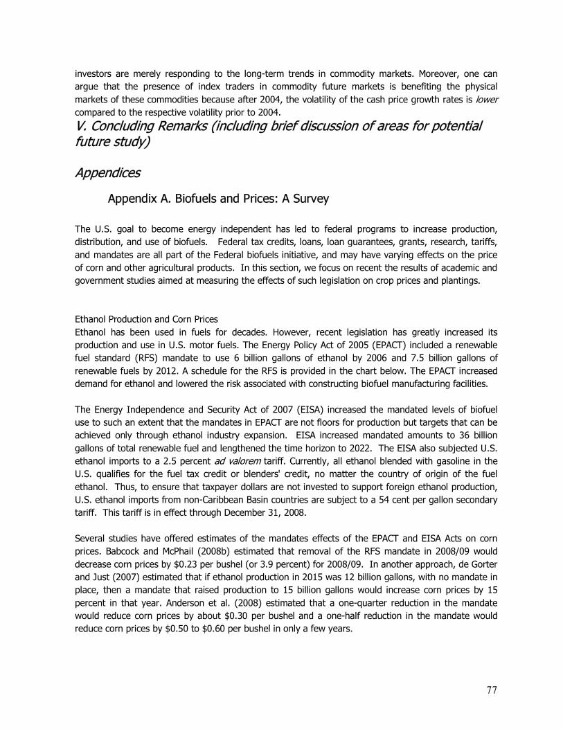
77

investors are merely responding to the long-term trends in commodity markets. Moreover, one can argue that the presence of index traders in commodity future markets is benefiting the physical markets of these commodities because after 2004, the volatility of the cash price growth rates is lower compared to the respective volatility prior to 2004.

V. Concluding Remarks (including brief discussion of areas for potential future study) Appendices

Appendix A. Biofuels and Prices: A Survey The U.S. goal to become energy independent has led to federal programs to increase production, distribution, and use of biofuels. Federal tax credits, loans, loan guarantees, grants, research, tariffs, and mandates are all part of the Federal biofuels initiative, and may have varying effects on the price of corn and other agricultural products. In this section, we focus on recent the results of academic and government studies aimed at measuring the effects of such legislation on crop prices and plantings. Ethanol Production and Corn Prices Ethanol has been used in fuels for decades. However, recent legislation has greatly increased its production and use in U.S. motor fuels. The Energy Policy Act of 2005 (EPACT) included a renewable fuel standard (RFS) mandate to use 6 billion gallons of ethanol by 2006 and 7.5 billion gallons of renewable fuels by 2012. A schedule for the RFS is provided in the chart below. The EPACT increased demand for ethanol and lowered the risk associated with constructing biofuel manufacturing facilities. The Energy Independence and Security Act of 2007 (EISA) increased the mandated levels of biofuel use to such an extent that the mandates in EPACT are not floors for production but targets that can be achieved only through ethanol industry expansion. EISA increased mandated amounts to 36 billion gallons of total renewable fuel and lengthened the time horizon to 2022. The EISA also subjected U.S. ethanol imports to a 2.5 percent ad valorem tariff. Currently, all ethanol blended with gasoline in the U.S. qualifies for the fuel tax credit or blenders' credit, no matter the country of origin of the fuel ethanol. Thus, to ensure that taxpayer dollars are not invested to support foreign ethanol production, U.S. ethanol imports from non-Caribbean Basin countries are subject to a 54 cent per gallon secondary tariff. This tariff is in effect through December 31, 2008. Several studies have offered estimates of the mandates effects of the EPACT and EISA Acts on corn prices. Babcock and McPhail (2008b) estimated that removal of the RFS mandate in 2008/09 would decrease corn prices by $0.23 per bushel (or 3.9 percent) for 2008/09. In another approach, de Gorter and Just (2007) estimated that if ethanol production in 2015 was 12 billion gallons, with no mandate in place, then a mandate that raised production to 15 billion gallons would increase corn prices by 15 percent in that year. Anderson et al. (2008) estimated that a one-quarter reduction in the mandate would reduce corn prices by about $0.30 per bushel and a one-half reduction in the mandate would reduce corn prices by $0.50 to $0.60 per bushel in only a few years.

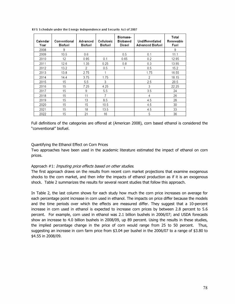
78

R F S S chedule under the E nergy Independence and S ecurity Act of 2007

Full definitions of the categories are offered at (American 2008), corn based ethanol is considered the �conventional� biofuel. Quantifying the Ethanol Effect on Corn Prices Two approaches have been used in the academic literature estimated the impact of ethanol on corn prices. Approach #1: Imputing price effects based on other studies. The first approach draws on the results from recent corn market projections that examine exogenous shocks to the corn market, and then infer the impacts of ethanol production as if it is an exogenous shock. Table 2 summarizes the results for several recent studies that follow this approach. In Table 2, the last column shows for each study how much the corn price increases on average for each percentage point increase in corn used in ethanol. The impacts on price differ because the models and the time periods over which the effects are measured differ. They suggest that a 10-percent increase in corn used in ethanol is expected to increase corn prices by between 2.8 percent to 5.6 percent. For example, corn used in ethanol was 2.1 billion bushels in 2006/07; and USDA forecasts show an increase to 4.0 billion bushels in 2008/09, up 89 percent. Using the results in these studies, the implied percentage change in the price of corn would range from 25 to 50 percent. Thus, suggesting an increase in corn farm price from $3.04 per bushel in the 2006/07 to a range of $3.80 to $4.55 in 2008/09.

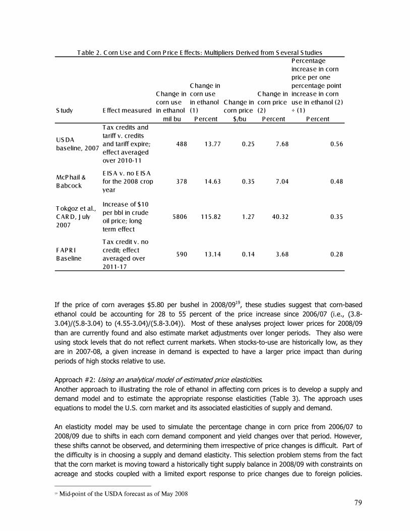
79

S tudy E ffect measured

C hange in corn use in ethanol

C hange in corn use in ethanol (1)

C hange in corn price

C hange in corn price (2)

P ercentage increase in corn price per one percentage point increase in corn use in ethanol (2) ÷ (1)

mil bu P ercent $/bu P ercent P ercent

US DA baseline, 2007

T ax credits and tariff v. credits and tariff expire; effect averaged over 2010-11

488 13.77 0.25 7.68 0.56

McP hail & Babcock

E IS A v. no E IS A for the 2008 crop year

378 14.63 0.35 7.04 0.48

T okgoz et al., C AR D, J uly 2007

Increase of $10 per bbl in crude oil price; long term effect

5806 115.82 1.27 40.32 0.35

F AP R I Baseline

T ax credit v. no credit; effect averaged over 2011-17

590 13.14 0.14 3.68 0.28

T able 2. C orn Use and C orn P rice E ffects: Multipliers Derived from S everal S tudies

If the price of corn averages $5.80 per bushel in 2008/0919, these studies suggest that corn-based ethanol could be accounting for 28 to 55 percent of the price increase since 2006/07 (i.e., (3.8-3.04)/(5.8-3.04) to (4.55-3.04)/(5.8-3.04)). Most of these analyses project lower prices for 2008/09 than are currently found and also estimate market adjustments over longer periods. They also were using stock levels that do not reflect current markets. When stocks-to-use are historically low, as they are in 2007-08, a given increase in demand is expected to have a larger price impact than during periods of high stocks relative to use. Approach #2: Using an analytical model of estimated price elasticities. Another approach to illustrating the role of ethanol in affecting corn prices is to develop a supply and demand model and to estimate the appropriate response elasticities (Table 3). The approach uses equations to model the U.S. corn market and its associated elasticities of supply and demand. An elasticity model may be used to simulate the percentage change in corn price from 2006/07 to 2008/09 due to shifts in each corn demand component and yield changes over that period. However, these shifts cannot be observed, and determining them irrespective of price changes is difficult. Part of the difficulty is in choosing a supply and demand elasticity. This selection problem stems from the fact that the corn market is moving toward a historically tight supply balance in 2008/09 with constraints on acreage and stocks coupled with a limited export response to price changes due to foreign policies.

19 Mid-point of the USDA forecast as of May 2008

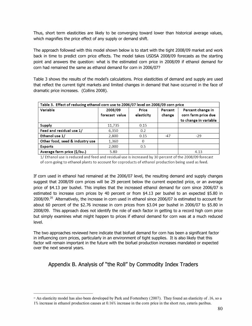
80

Thus, short term elasticities are likely to be converging toward lower than historical average values, which magnifies the price effect of any supply or demand shift. The approach followed with this model shown below is to start with the tight 2008/09 market and work back in time to predict corn price effects. The model takes USDSA 2008/09 forecasts as the starting point and answers the question: what is the estimated corn price in 2008/09 if ethanol demand for corn had remained the same as ethanol demand for corn in 2006/07? Table 3 shows the results of the model�s calculations. Price elasticities of demand and supply are used that reflect the current tight markets and limited changes in demand that have occurred in the face of dramatic price increases. (Collins 2008).

If corn used in ethanol had remained at the 2006/07 level, the resulting demand and supply changes suggest that 2008/09 corn prices will be 29 percent below the current expected price, or an average price of $4.13 per bushel. This implies that the increased ethanol demand for corn since 2006/07 is estimated to increase corn prices by 40 percent or from $4.13 per bushel to an expected $5.80 in 2008/09.20 Alternatively, the increase in corn used in ethanol since 2006/07 is estimated to account for about 60 percent of the $2.76 increase in corn prices from $3.04 per bushel in 2006/07 to $5.80 in 2008/09. This approach does not identify the role of each factor in getting to a record high corn price but simply examines what might happen to prices if ethanol demand for corn was at a much reduced level. The two approaches reviewed here indicate that biofuel demand for corn has been a significant factor in influencing corn prices, particularly in an environment of tight supplies. It is also likely that this factor will remain important in the future with the biofuel production increases mandated or expected over the next several years.

Appendix B. Analysis of �the Roll� by Commodity Index Traders

20 An elasticity model has also been developed by Park and Fortenbery (2007). They found an elasticity of .16, so a 1% increase in ethanol production causes at 0.16% increase in the corn price in the short run, ceteris paribus.

81

The objective of this analysis is to study the effects of Commodity Index Traders� (CITs) rolling strategies on the spread between the nearby and next-to-nearby contract, and on the volatility of this spread. Standard time series analysis reveals that the spread is characterized by two types of seasonality. The first one is the contract month-effect, and we modeled it with simple dummy variables which are equal to one for that contract and zero otherwise. Within each contract, there is also a marked chronological pattern in the spread, which is consistent with the cost-of-carry relationship. We, therefore, introduced a variable that counts the number of trading days left in each contract before expiration. To measure rolling activity by CITs we constructed a variable equal to negative one times the change in the net position of CITs in the nearby contract from the previous day.21 Net positions are calculated as long futures + long adjusted options � (short futures + short adjusted options). We analyze three markets: wheat, corn and soy beans. We filtered out days for which price limits affected the markets. To avoid delivery distortion, we also eliminated the last week of transactions in each contract. For soy beans, we only report the contract months for which CITs held significant positions.22 Standards diagnostic tests indicate that the residuals exhibit time varying conditional volatility and serial correlation. We therefore employ standard GARCH model to best captures the dynamic of the spread in both the conditional mean and the conditional variance

ttiittt

t

ttttiit

RollXhLLh

hRollXs

θλβεαωε

εδγµ

++++=

Φ+++=

,2

2/1,

)()(

)1,0(~

where Xi,t contains the variables used to deseasonalize the conditional mean and variance, while Rollt refers to the rolling variable.23 As estimation method we adopt a quasi-maximum likelihood which allows to compute robust standard errors. Therefore, the distribution of the error term is assumed to be normal with zero mean and unit variance. The main findings are as follows. Table A.1 reports the effects of the Roll and the variables in Xi,t on the spread. In all three markets we find that the CIT�s rolling strategies increase the spread. This is to be expected. During the rolling period CITs sell the nearby contract, causing the price to fall, and buy the next-to-nearby contract, which cause the price of this contract to increase. The magnitude of this effect is different for the three markets analyzed. The effect in the wheat market is considerably larger than in the other two markets. The coefficient of .0025

21 We multiply by -1 to make the roll a positive number on most dates, which in turn simplifies interpretation of the coefficients in Tables A.1 and A.2. 22 There is some small amount of rolling into, and out of, the August and September soy contracts. The coefficient on the roll is very similar (it differs by only 5%) when all months are included 23 To test for endogeneity, we run the standard Granger non-causality test between the spread and the rolling variable and found that there is not feedback effect from the spread to the rolling variable. In fact, principal rolling strategies and timing is known well in advanced by market participants.

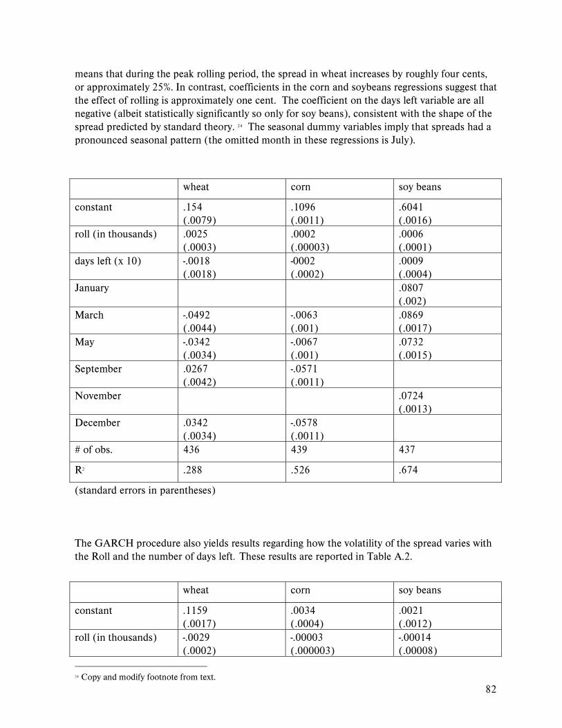
82

means that during the peak rolling period, the spread in wheat increases by roughly four cents, or approximately 25%. In contrast, coefficients in the corn and soybeans regressions suggest that the effect of rolling is approximately one cent. The coefficient on the days left variable are all negative (albeit statistically significantly so only for soy beans), consistent with the shape of the spread predicted by standard theory. 24 The seasonal dummy variables imply that spreads had a pronounced seasonal pattern (the omitted month in these regressions is July).

wheat corn soy beans

constant .154 (.0079)

.1096 (.0011)

.6041 (.0016)

roll (in thousands) .0025 (.0003)

.0002 (.00003)

.0006 (.0001)

days left (x 10) -.0018 (.0018)

-0002 (.0002)

.0009 (.0004)

January .0807 (.002)

March -.0492 (.0044)

-.0063 (.001)

.0869 (.0017)

May -.0342 (.0034)

-.0067 (.001)

.0732 (.0015)

September .0267 (.0042)

-.0571 (.0011)

November .0724 (.0013)

December .0342 (.0034)

-.0578 (.0011)

# of obs. 436 439 437

R2 .288 .526 .674

(standard errors in parentheses)

The GARCH procedure also yields results regarding how the volatility of the spread varies with the Roll and the number of days left. These results are reported in Table A.2.

wheat corn soy beans

constant .1159 (.0017)

.0034 (.0004)

.0021 (.0012)

roll (in thousands) -.0029 (.0002)

-.00003 (.000003)

-.00014 (.00008)

24 Copy and modify footnote from text.

83

days left (x 10) -.0209 (.0001)

-00005 (.000003)

.00003 (.0003)

GARCH (-1) 77.28 (1.98)

40.12 (6.98)

44.63 (11.41)

Residuals(-1)2 17.25 (5.53)

53.671 (9.7)

50.75 (12.96)

# of obs. 436 439 437

(standard errors in parentheses. all coefficients are multiplied by 100 for ease of presentation)

The coefficients in Table A.2 imply that the CITs� rolling strategies reduce volatility. For example, in the wheat regression, the coefficient of .000029 means that during the peak rolling period, volatility falls by roughly .0004, which is approximately 30% of average volatility. We conjecture that when rolling is high, total volume in the market is high, and this greater liquidity induces less volatility.

Appendix C. Analysis of commodities with and without futures markets This note offers a comparison of the behavior of cash (spot) prices across metals and energy commodities with and without futures markets. To compare the two commodity classes, I construct two indices that reflect the average cash price growth rates of the two classes. I consider monthly, quarterly, and annual spot price growth rates. I focus on lower frequency growth rates, as opposed to daily ones, to capture the long-run movements in these commodity markets. Over the period 1998 to 2008, I find that on average the non-traded commodities have experienced a higher cash price appreciation than the traded commodities but this price appreciation differential is not statistically significant. More importantly, comparing the price growth rates over the 1998 to 2003 period to the period from 2004 to 2008, I find that on average the price growth rates of both commodity classes are substantially higher in the latter period. This structural change in the growth rate levels is economically and statistically significant. It is present in the growth rate of price indices for traded and non-traded commodities at the quarterly and annual frequency. It is also present in the annual and quarterly spot price growth rates of most individual commodities within the metals and energy commodity class. Finally, the structural break finding is very robust because it extends to other commodity classes like agricultural products. Overall, the current results indicate that the pattern in price behavior in commodities with and without futures markets has been very similar over the past 10 years. Specifically, the large boom in commodity prices that we have seen since 2004 has been experienced by both traded and non-traded commodities. The year 2004 is important because it is believed that this is the year when commodity index funds became extremely popular.25 The fact that index traders became an important trader 25 Information available to the CFTC and in the financial press suggests that there may have been a change in commodity index investing in this year.

84

category in futures market raises the question of whether they are causing the recent spike in commodity spot prices. However, the finding that both traded and non-traded commodities experienced a structural break at 2004 casts doubts on the conjecture that index trading is having a long-term impact on the physical commodity market. The rest of the note is organized as follows. In Section 2, I describe the commodity data I use and how I construct various growth rates of spot price indices. In Section 3 to 5, I present graphical evidence for the behavior of the spot price growth rate indices for traded and non-traded commodities. In Section 6, I discuss a series of robustness tests of the reported findings, while in Section 7, I measure their statistical significance. Finally, in Section 8, I discuss how the findings of the study can be used to shed light on the possible impact of financial investors on the physical commodity markets. 2. Data and Methodology The daily spot price data are collected from Bloomberg. In most of this study, I focus on metals and energy commodities. These commodities have been used in a recent report by Deutsche Bank.26 In particular, the class of traded commodities (i.e. commodities with established futures markets) includes gold, copper, silver, aluminum lead, nickel, tin, zinc, natural gas, and west Texas intermediate oil (WTI). Table 1: Descriptive Statistics for Growth Rate of Price Indices

26 Commodities Special, �Commodities and the Role of Speculators,� May 9, 2008, Deutsche Bank, Global Markets Research, Commodities Research.

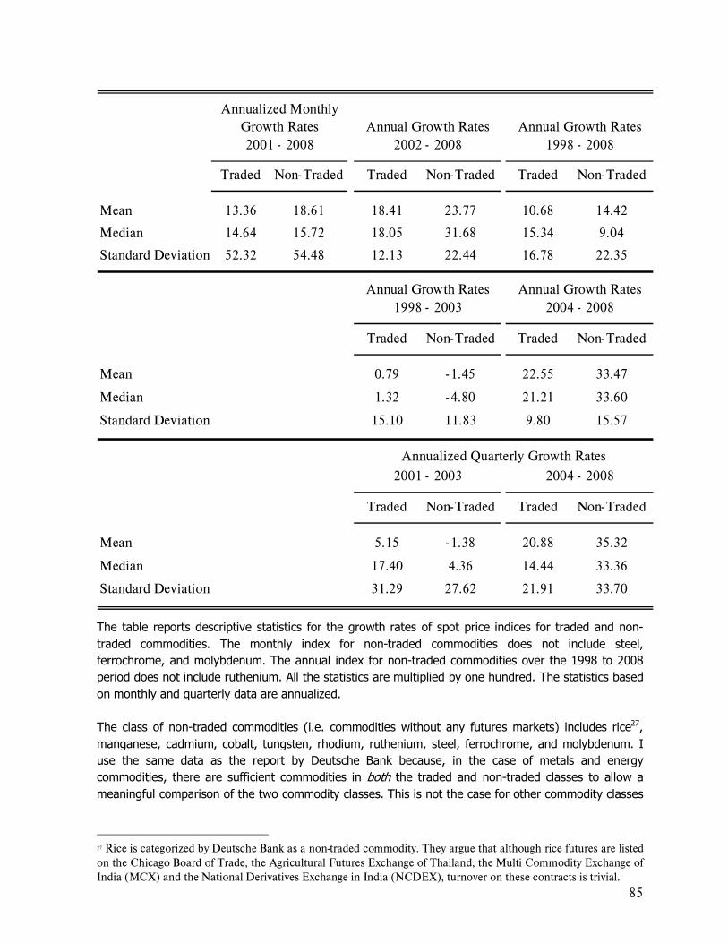
85

Traded Non- Traded Traded Non-Traded Traded Non- Traded

Mean 13.36 18.61 18.41 23.77 10.68 14.42

Median 14.64 15.72 18.05 31.68 15.34 9.04

Standard Deviation 52.32 54.48 12.13 22.44 16.78 22.35

Traded Non-Traded Traded Non- Traded

Mean 0.79 -1.45 22.55 33.47

Median 1.32 -4.80 21.21 33.60

Standard Deviation 15.10 11.83 9.80 15.57

Traded Non-Traded Traded Non- Traded

Mean 5.15 -1.38 20.88 35.32

Median 17.40 4.36 14.44 33.36

Standard Deviation 31.29 27.62 21.91 33.70

Annualized Quarterly Growth Rates

Annual Growth Rates1998 - 20082001 - 2008

1998 - 2003

Annualized Monthly Growth Rates Annual Growth Rates

2002 - 2008

2001 - 2003 2004 - 2008

Annual Growth Rates2004 - 2008

Annual Growth Rates

The table reports descriptive statistics for the growth rates of spot price indices for traded and non-traded commodities. The monthly index for non-traded commodities does not include steel, ferrochrome, and molybdenum. The annual index for non-traded commodities over the 1998 to 2008 period does not include ruthenium. All the statistics are multiplied by one hundred. The statistics based on monthly and quarterly data are annualized. The class of non-traded commodities (i.e. commodities without any futures markets) includes rice27, manganese, cadmium, cobalt, tungsten, rhodium, ruthenium, steel, ferrochrome, and molybdenum. I use the same data as the report by Deutsche Bank because, in the case of metals and energy commodities, there are sufficient commodities in both the traded and non-traded classes to allow a meaningful comparison of the two commodity classes. This is not the case for other commodity classes

27 Rice is categorized by Deutsche Bank as a non-traded commodity. They argue that although rice futures are listed on the Chicago Board of Trade, the Agricultural Futures Exchange of Thailand, the Multi Commodity Exchange of India (MCX) and the National Derivatives Exchange in India (NCDEX), turnover on these contracts is trivial.

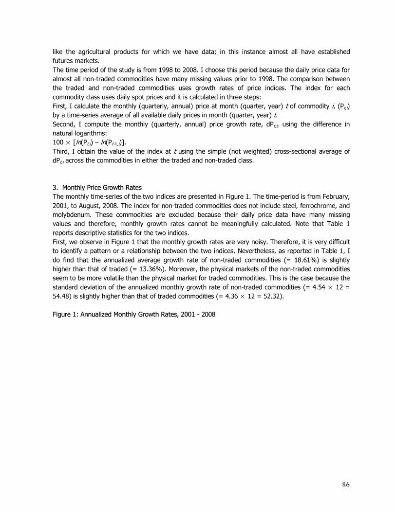
86

like the agricultural products for which we have data; in this instance almost all have established futures markets. The time period of the study is from 1998 to 2008. I choose this period because the daily price data for almost all non-traded commodities have many missing values prior to 1998. The comparison between the traded and non-traded commodities uses growth rates of price indices. The index for each commodity class uses daily spot prices and it is calculated in three steps: First, I calculate the monthly (quarterly, annual) price at month (quarter, year) t of commodity i, (Pt,i) by a time-series average of all available daily prices in month (quarter, year) t. Second, I compute the monthly (quarterly, annual) price growth rate, dPt,i, using the difference in natural logarithms: 100 × [ln(Pt,i) � ln(Pt-1,i)]. Third, I obtain the value of the index at t using the simple (not weighted) cross-sectional average of dPt,i across the commodities in either the traded and non-traded class. 3. Monthly Price Growth Rates The monthly time-series of the two indices are presented in Figure 1. The time-period is from February, 2001, to August, 2008. The index for non-traded commodities does not include steel, ferrochrome, and molybdenum. These commodities are excluded because their daily price data have many missing values and therefore, monthly growth rates cannot be meaningfully calculated. Note that Table 1 reports descriptive statistics for the two indices. First, we observe in Figure 1 that the monthly growth rates are very noisy. Therefore, it is very difficult to identify a pattern or a relationship between the two indices. Nevertheless, as reported in Table 1, I do find that the annualized average growth rate of non-traded commodities (= 18.61%) is slightly higher than that of traded (= 13.36%). Moreover, the physical markets of the non-traded commodities seem to be more volatile than the physical market for traded commodities. This is the case because the standard deviation of the annualized monthly growth rate of non-traded commodities (= 4.54 × 12 = 54.48) is slightly higher than that of traded commodities (= 4.36 × 12 = 52.32). Figure 1: Annualized Monthly Growth Rates, 2001 - 2008

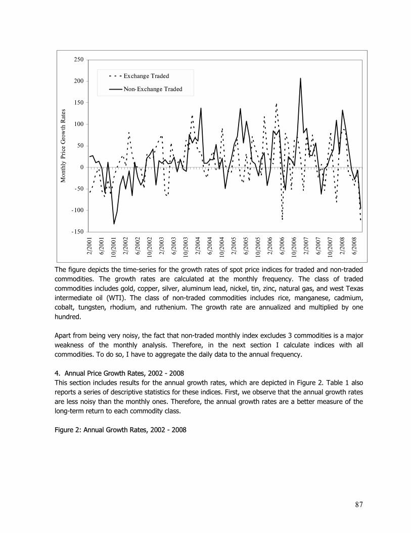
87

- 150

- 100

- 50

0

50

100

150

200

250

2/20

01

6/20

01

10/2

001

2/20

02

6/20

02

10/2

002

2/20

03

6/20

03

10/2

003

2/20

04

6/20

04

10/2

004

2/20

05

6/20

05

10/2

005

2/20

06

6/20

06

10/2

006

2/20

07

6/20

07

10/2

007

2/20

08

6/20

08

Mon

thly

Pri

ce G

row

th R

ates

Exchange Traded

Non- Exchange Traded

The figure depicts the time-series for the growth rates of spot price indices for traded and non-traded commodities. The growth rates are calculated at the monthly frequency. The class of traded commodities includes gold, copper, silver, aluminum lead, nickel, tin, zinc, natural gas, and west Texas intermediate oil (WTI). The class of non-traded commodities includes rice, manganese, cadmium, cobalt, tungsten, rhodium, and ruthenium. The growth rate are annualized and multiplied by one hundred. Apart from being very noisy, the fact that non-traded monthly index excludes 3 commodities is a major weakness of the monthly analysis. Therefore, in the next section I calculate indices with all commodities. To do so, I have to aggregate the daily data to the annual frequency. 4. Annual Price Growth Rates, 2002 - 2008 This section includes results for the annual growth rates, which are depicted in Figure 2. Table 1 also reports a series of descriptive statistics for these indices. First, we observe that the annual growth rates are less noisy than the monthly ones. Therefore, the annual growth rates are a better measure of the long-term return to each commodity class. Figure 2: Annual Growth Rates, 2002 - 2008

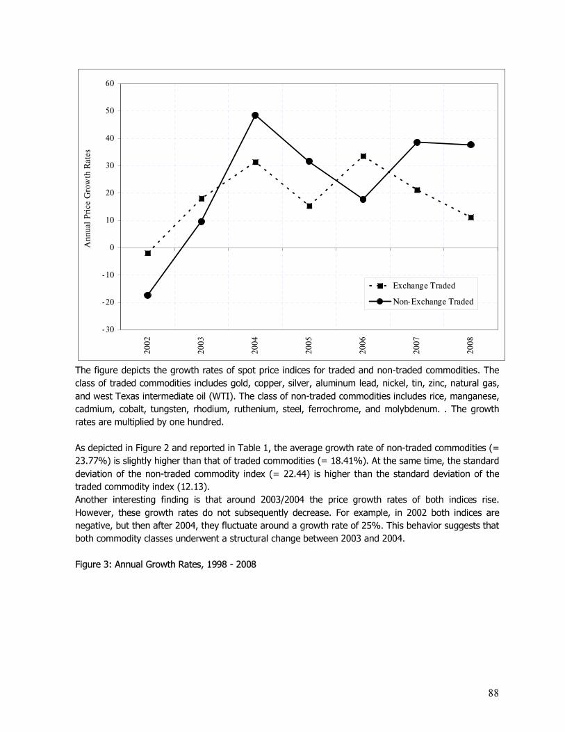
88

- 30

- 20

- 10

0

10

20

30

40

50

60

2002

2003

2004

2005

2006

2007

2008

Exchange Traded

Non-Exchange Traded

Ann

ual

Pri

ce G

row

th R

ates

The figure depicts the growth rates of spot price indices for traded and non-traded commodities. The class of traded commodities includes gold, copper, silver, aluminum lead, nickel, tin, zinc, natural gas, and west Texas intermediate oil (WTI). The class of non-traded commodities includes rice, manganese, cadmium, cobalt, tungsten, rhodium, ruthenium, steel, ferrochrome, and molybdenum. . The growth rates are multiplied by one hundred. As depicted in Figure 2 and reported in Table 1, the average growth rate of non-traded commodities (= 23.77%) is slightly higher than that of traded commodities (= 18.41%). At the same time, the standard deviation of the non-traded commodity index (= 22.44) is higher than the standard deviation of the traded commodity index (12.13). Another interesting finding is that around 2003/2004 the price growth rates of both indices rise. However, these growth rates do not subsequently decrease. For example, in 2002 both indices are negative, but then after 2004, they fluctuate around a growth rate of 25%. This behavior suggests that both commodity classes underwent a structural change between 2003 and 2004. Figure 3: Annual Growth Rates, 1998 - 2008

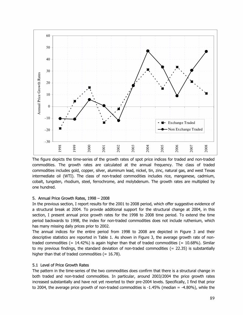
89

- 30

- 20

- 10

0

10

20

30

40

50

60

199

8

199

9

200

0

200

1

200

2

200

3

200

4

200

5

200

6

200

7

200

8

Exchange Traded

Non Exchange Traded

An

nual

Pri

ce G

row

th R

ates

The figure depicts the time-series of the growth rates of spot price indices for traded and non-traded commodities. The growth rates are calculated at the annual frequency. The class of traded commodities includes gold, copper, silver, aluminum lead, nickel, tin, zinc, natural gas, and west Texas intermediate oil (WTI). The class of non-traded commodities includes rice, manganese, cadmium, cobalt, tungsten, rhodium, steel, ferrochrome, and molybdenum. The growth rates are multiplied by one hundred. 5. Annual Price Growth Rates, 1998 � 2008 In the previous section, I report results for the 2001 to 2008 period, which offer suggestive evidence of a structural break at 2004. To provide additional support for the structural change at 2004, in this section, I present annual price growth rates for the 1998 to 2008 time period. To extend the time period backwards to 1998, the index for non-traded commodities does not include ruthenium, which has many missing daily prices prior to 2002. The annual indices for the entire period from 1998 to 2008 are depicted in Figure 3 and their descriptive statistics are reported in Table 1. As shown in Figure 3, the average growth rate of non-traded commodities (= 14.42%) is again higher than that of traded commodities (= 10.68%). Similar to my previous findings, the standard deviation of non-traded commodities (= 22.35) is substantially higher than that of traded commodities (= 16.78). 5.1 Level of Price Growth Rates The pattern in the time-series of the two commodities does confirm that there is a structural change in both traded and non-traded commodities. In particular, around 2003/2004 the price growth rates increased substantially and have not yet reverted to their pre-2004 levels. Specifically, I find that prior to 2004, the average price growth of non-traded commodities is -1.45% (median = -4.80%), while the

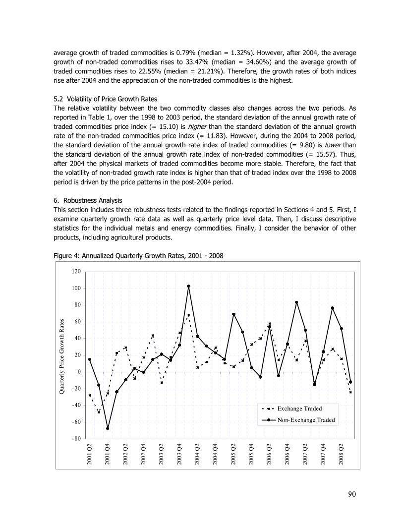
90

average growth of traded commodities is 0.79% (median = 1.32%). However, after 2004, the average growth of non-traded commodities rises to 33.47% (median = 34.60%) and the average growth of traded commodities rises to 22.55% (median = 21.21%). Therefore, the growth rates of both indices rise after 2004 and the appreciation of the non-traded commodities is the highest. 5.2 Volatility of Price Growth Rates The relative volatility between the two commodity classes also changes across the two periods. As reported in Table 1, over the 1998 to 2003 period, the standard deviation of the annual growth rate of traded commodities price index (= 15.10) is higher than the standard deviation of the annual growth rate of the non-traded commodities price index (= 11.83). However, during the 2004 to 2008 period, the standard deviation of the annual growth rate index of traded commodities (= 9.80) is lower than the standard deviation of the annual growth rate index of non-traded commodities (= 15.57). Thus, after 2004 the physical markets of traded commodities become more stable. Therefore, the fact that the volatility of non-traded growth rate index is higher than that of traded index over the 1998 to 2008 period is driven by the price patterns in the post-2004 period. 6. Robustness Analysis This section includes three robustness tests related to the findings reported in Sections 4 and 5. First, I examine quarterly growth rate data as well as quarterly price level data. Then, I discuss descriptive statistics for the individual metals and energy commodities. Finally, I consider the behavior of other products, including agricultural products. Figure 4: Annualized Quarterly Growth Rates, 2001 - 2008

- 80

- 60

- 40

- 20

0

20

40

60

80

100

120

200

1 Q

2

200

1 Q

4

200

2 Q

2

200

2 Q

4

200

3 Q

2

200

3 Q

4

200

4 Q

2

200

4 Q

4

200

5 Q

2

200

5 Q

4

200

6 Q

2

200

6 Q

4

200

7 Q

2

200

7 Q

4

200

8 Q

2

Exchange Traded

Non-Exchange Traded

Qua

rter

ly P

rice

Gro

wth

Rat

es

91

The figure depicts the growth rates of indices for traded and non-traded commodities. The growth rates are calculated at the quarterly frequency. The class of traded commodities includes gold, copper, silver, aluminum lead, nickel, tin, zinc, natural gas, and west Texas intermediate oil (WTI). The class of non-traded commodities includes rice, manganese, cadmium, cobalt, tungsten, rhodium, ruthenium, steel, and molybdenum. The growth rates are annualized and multiplied by a hundred. 6.1 Quarterly Data To begin with, I further examine the timing of the structural break in the levels of the spot price growth rates. In Figure 4, I plot the time-series of the annualized quarterly growth rates of my two indices. The figure shows that the prices of both non-traded and traded commodities grew steadily from 2003(Q3) to 2004(Q1). In particular, the annualized quarterly growth rates for both indices is below 20% at 2003(Q3), and by the first quarter of 2004, they both rise above 60%. Figure 5: Quarterly Price Indices, 2001 - 2008

0

100

200

300

400

500

600

200

1 Q

2

200

1 Q

4

200

2 Q

2

200

2 Q

4

200

3 Q

2

200

3 Q

4

200

4 Q

2

200

4 Q

4

200

5 Q

2

200

5 Q

4

200

6 Q

2

200

6 Q

4

200

7 Q

2

200

7 Q

4

200

8 Q

2

Exchange Traded

Non-Exchange Traded

Qu

arte

rly

Pri

ce L

evel

s

The figure depicts spot price indices for traded and non-traded commodities. The indices are calculated at the quarterly frequency. The class of traded commodities includes gold, copper, silver, aluminum lead, nickel, tin, zinc, natural gas, and west Texas intermediate oil (WTI). The class of non-traded commodities includes rice, manganese, cadmium, cobalt, tungsten, rhodium, ruthenium, steel, and molybdenum. The price level index is calculated as follows. First, I calculate the quarterly price at quarter t of commodity i, (Pt,i) by a time-series average of all available daily prices in quarter t. Second, I compute the price level index for quarter t with a simple (not weighted) average of Pt,i across the commodities in either the traded and non-traded class. Finally, I normalize the index using its value at 2001(Q2). Table 2: Mean and Median Price Growth Rates for Metals and Energy Commodities

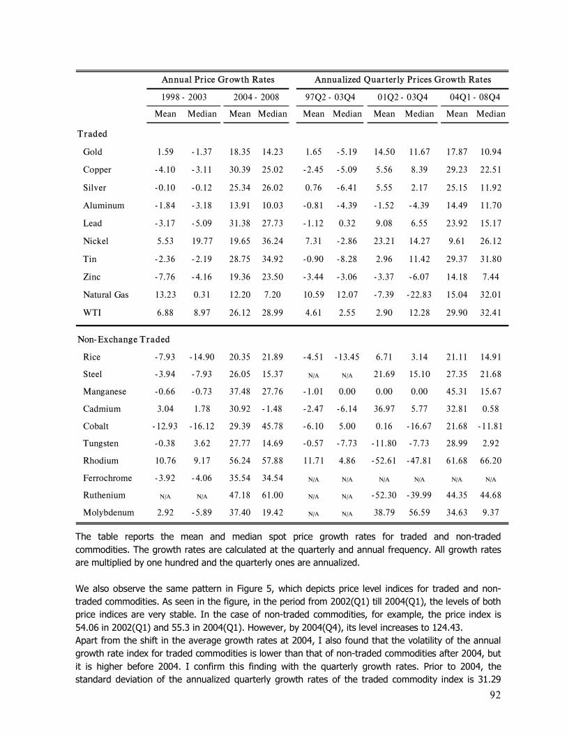
92

Mean Median Mean Median Mean Median Mean Median Mean Median

Traded

Gold 1.59 - 1.37 18.35 14.23 1.65 - 5.19 14.50 11.67 17.87 10.94

Copper - 4.10 - 3.11 30.39 25.02 - 2.45 - 5.09 5.56 8.39 29.23 22.51

Silver - 0.10 - 0.12 25.34 26.02 0.76 - 6.41 5.55 2.17 25.15 11.92

Aluminum - 1.84 - 3.18 13.91 10.03 - 0.81 - 4.39 - 1.52 - 4.39 14.49 11.70

Lead - 3.17 - 5.09 31.38 27.73 - 1.12 0.32 9.08 6.55 23.92 15.17

Nickel 5.53 19.77 19.65 36.24 7.31 - 2.86 23.21 14.27 9.61 26.12

Tin - 2.36 - 2.19 28.75 34.92 - 0.90 - 8.28 2.96 11.42 29.37 31.80

Zinc - 7.76 - 4.16 19.36 23.50 - 3.44 - 3.06 - 3.37 - 6.07 14.18 7.44

Natural Gas 13.23 0.31 12.20 7.20 10.59 12.07 - 7.39 - 22.83 15.04 32.01

WTI 6.88 8.97 26.12 28.99 4.61 2.55 2.90 12.28 29.90 32.41

Non- Exchange Traded

Rice - 7.93 - 14.90 20.35 21.89 - 4.51 - 13.45 6.71 3.14 21.11 14.91

Steel - 3.94 - 7.93 26.05 15.37 N/A N/A 21.69 15.10 27.35 21.68

Manganese - 0.66 - 0.73 37.48 27.76 - 1.01 0.00 0.00 0.00 45.31 15.67

Cadmium 3.04 1.78 30.92 - 1.48 - 2.47 - 6.14 36.97 5.77 32.81 0.58

Cobalt - 12.93 - 16.12 29.39 45.78 - 6.10 5.00 0.16 - 16.67 21.68 - 11.81

Tungsten - 0.38 3.62 27.77 14.69 - 0.57 - 7.73 - 11.80 - 7.73 28.99 2.92

Rhodium 10.76 9.17 56.24 57.88 11.71 4.86 - 52.61 - 47.81 61.68 66.20

Ferrochrome - 3.92 - 4.06 35.54 34.54 N/A N/A N/A N/A N/A N/A

Ruthenium N/A N/A 47.18 61.00 N/A N/A - 52.30 - 39.99 44.35 44.68

Molybdenum 2.92 - 5.89 37.40 19.42 N/A N/A 38.79 56.59 34.63 9.37

97Q2 - 03Q4 04Q1 - 08Q4

Annual Price Growth Rates Annualized Quarter ly Pr ices Growth Rates

1998 - 2003 2004 - 2008 01Q2 - 03Q4

The table reports the mean and median spot price growth rates for traded and non-traded commodities. The growth rates are calculated at the quarterly and annual frequency. All growth rates are multiplied by one hundred and the quarterly ones are annualized. We also observe the same pattern in Figure 5, which depicts price level indices for traded and non-traded commodities. As seen in the figure, in the period from 2002(Q1) till 2004(Q1), the levels of both price indices are very stable. In the case of non-traded commodities, for example, the price index is 54.06 in 2002(Q1) and 55.3 in 2004(Q1). However, by 2004(Q4), its level increases to 124.43. Apart from the shift in the average growth rates at 2004, I also found that the volatility of the annual growth rate index for traded commodities is lower than that of non-traded commodities after 2004, but it is higher before 2004. I confirm this finding with the quarterly growth rates. Prior to 2004, the standard deviation of the annualized quarterly growth rates of the traded commodity index is 31.29

93

and it is higher than that of the non-traded commodities (= 27.62). After 2004, the standard deviation of the quarterly index for traded commodities is 21.91 and it is lower than that of the non-traded (= 33.70). These statistics are reported in the last row of Table 1. 6.2 Spot Price Growth Rates of Individual Metals and Energy Commodities In most of the analysis I use the growth rates of indices. To ensure that the documented shift in the levels of these indices is not driven by one or a couple of commodities, I also examine spot price growth rates for individual commodities. Specifically, in Table 2, I report the mean and median of annual and quarterly spot price growth rates for individual commodities. The annual growth rates are computed for two periods: 1998 to 2003, and 2004 to 2008. The quarterly growth rates are annualized and computed for three periods: 1997Q2 to 2003Q4, 2001Q2 to 2003Q4, and 2004Q1 to 2008Q3. The mean and median growth rates in Table 2 show that the structural break in 2004 is a widespread phenomenon across most commodities. For example, the mean annual price growth rate of WTI before 2004 is 6.88%, while after 2004 it rises to 26.12%. Natural gas, cadmium, and molybdenum, are the only commodities for which the mean and median do not both rise after 2004. 6.3 Other Commodities A final robustness test is to examine whether commodities, other than energy and metals, have also experienced a structural change in 2004. Therefore, in Table 3, I report annual and quarterly growth rates for forest products (lumber, plywood, oriented strand board), livestock (steers, hogs, broilers), agricultural products (corn, wheat, soybeans, coffee), and textiles (cotton, burlap). I also consider platinum and additional energy products (Brent crude oil, gasoline, heating oil). I find that the price growth rates of forest products are negative in the post-2004 period and in most cases they are lower compared to the pre-2004 period. For example, the mean annual price growth rate of plywood before 2004 is 3.16, while after 2004 it decreases to -2.67. This finding is not surprising due to the slow down in the real estate market, which absorbs most of the forest products. Table 3: Mean and Median Price Growth Rates for Additional Commodities

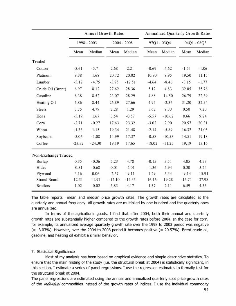
94

Mean Median Mean Median Mean Median Mean Median

Traded

Cotton - 3.61 - 5.71 2.68 2.21 -0.69 4.62 -1.51 - 1.06

Platinum 9.38 1.68 20.72 20.02 10.90 8.95 19.50 11.15

Lumber - 5.12 - 4.75 - 3.75 - 12.51 -4.64 -8.46 -3.15 - 1.77

Crude Oil (Brent) 6.97 8.12 27.62 28.36 5.12 4.83 32.05 35.76

Gasoline 6.38 8.52 23.07 28.29 4.88 14.50 26.79 22.39

Heating Oil 6.86 8.44 26.89 27.66 4.95 -2.36 31.20 32.54

Steers 3.75 4.79 2.28 1.29 5.62 8.33 0.50 7.20

Hogs - 5.19 1.67 3.54 - 0.57 -5.57 - 10.62 8.66 9.84

Corn - 2.71 - 0.27 17.63 23.32 -3.03 2.90 20.57 20.31

Wheat - 1.33 1.15 19.34 21.48 -2.14 -5.89 16.32 21.05

Soybeans - 3.06 - 1.08 14.99 17.37 -0.58 - 10.53 14.51 19.18

Coffee -23.32 - 24.30 19.19 17.65 - 18.02 - 11.25 19.19 13.16

Non-Exchange Traded

Burlap 0.35 - 0.36 5.23 4.78 -0.15 3.51 4.05 4.53

Hides - 0.81 - 0.68 0.01 - 2.01 -1.36 5.94 0.30 3.24

Plywood 3.16 0.06 - 2.67 - 9.11 7.29 5.34 -9.14 - 15.91

Strand Board 12.31 11.97 - 12.10 - 14.35 16.16 19.28 - 15.71 - 37.98

Broilers 1.02 - 0.02 5.83 4.17 1.37 2.11 6.59 4.53

Annual Growth Rates Annualized Quarter ly Growth Rates

1998 - 2003 2004 - 2008 97Q1 - 03Q4 04Q1 - 08Q3

The table reports mean and median price growth rates. The growth rates are calculated at the quarterly and annual frequency. All growth rates are multiplied by one hundred and the quarterly ones are annualized. In terms of the agricultural goods, I find that after 2004, both their annual and quarterly growth rates are substantially higher compared to the growth rates before 2004. In the case for corn, for example, its annualized average quarterly growth rate over the 1998 to 2003 period was negative (= -3.03%). However, over the 2004 to 2008 period it becomes positive (= 20.57%). Brent crude oil, gasoline, and heating oil exhibit a similar behavior. 7. Statistical Significance Most of my analysis has been based on graphical evidence and simple descriptive statistics. To ensure that the main finding of the study (i.e. the structural break at 2004) is statistically significant, in this section, I estimate a series of panel regressions. I use the regression estimates to formally test for the structural break at 2004. The panel regressions are estimated using the annual and annualized quarterly spot price growth rates of the individual commodities instead of the growth rates of indices. I use the individual commodity

95

data to exploit all their time-series and cross-sectional variation. This approach is more efficient than estimating the panel regressions with the growth rates of the indices because the indices smooth out cross-sectional differences within the traded and non-traded commodity classes. In the case of the annual growth rates, dPt,i, I estimate three panel regressions. The regression include a series of dummy variables, which are designed to test whether there are differences between traded and non-traded commodities, and differences in the levels of price growth rates before and after 2004. The regressions models are: dPt,i = α1DTR + α2DNTR + β1dPt-1,i dPt,i = α3D03 + α4D04 + β2dPt-1,i dPt,i = α5(DTR × D03) + α6(DTR× D04) + α7(DNTR× D03) + α8(DNTR × D04) + β3dPt-1,i In the above regressions, DTR is a dummy variable that takes the value of one if commodity i is traded, and zero otherwise. Similarly, DNTR is a dummy variable that takes the value of one if commodity i is not traded, and zero otherwise. D03 (D04) is a dummy variable that takes the value of one if year t is prior (after) to 2004, and zero otherwise. Table 4: Panel OLS Regressions

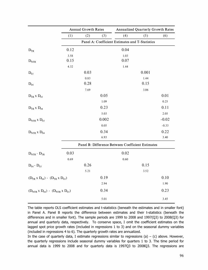
96

(1) (2) (3) (4) (5) (6)

DTR 0.12 0.04

3.58 1.03

DNTR 0.15 0.07

4.32 1.44

D03 0.03 0.001

0.83 1.44

D04 0.28 0.15

7.69 3.06

DTR x D03 0.05 0.01

1.09 0.25

DTR x D04 0.23 0.11

5.03 2.05

DNTR x D03 0.002 - 0.02

0.05 - 0.33

DNTR x D04 0.34 0.226.93 3.40

DNTR - DTR 0.03 0.02

0.69 0.60

D04 - D03 0.26 0.15

5.21 3.52

(DTR x D04) - (DTR x D03) 0.19 0.10

2.94 1.90

(DNTR x D04) - (DNTR x D03) 0.34 0.23

5.01 3.45

Panel A: Coefficient Estimates and T- Statistics

Panel B: Difference Between Coefficient Estimates

Annualized Quarter ly Growth RatesAnnual Growth Rates

The table reports OLS coefficient estimates and t-statistics (beneath the estimates and in smaller font) in Panel A. Panel B reports the difference between estimates and their t-statistics (beneath the differences and in smaller font). The sample periods are 1999 to 2008 and 1997(Q3) to 2008(Q3) for annual and quarterly data, respectively. To conserve space, I omit the coefficient estimates on the lagged spot price growth rates (included in regressions 1 to 3) and on the seasonal dummy variables (included in regressions 4 to 6). The quarterly growth rates are annualized. In the case of quarterly data, I estimate regressions similar to regressions (a) � (c) above. However, the quarterly regressions include seasonal dummy variables for quarters 1 to 3. The time period for annual data is 1999 to 2008 and for quarterly data is 1997Q3 to 2008Q3. The regressions are

97

estimated with OLS and the estimation results are reported in Table 4. The results with annual growth rates are in columns 1 to 3, while the results with quarterly data are in columns 4 to 6. 7.1 Traded versus Non-Traded In columns 1 and 4 of Table 4, I report the estimation results of the type (a) regression presented above. In both the annual and quarterly regressions, I find that the coefficient estimates on the DTR and DNTR dummy variables are very similar and not statistically different. For example, in the case of the annual data, the estimates on DTR and DNTR, reported in Panel A, are 0.12 and 0.13, respectively. Moreover, their difference, 0.03, is not statistically different from zero; its t-statistics is only 0.69. See Table 4, Panel B. Therefore, there is no evidence that the mean growth rate between traded and non-traded commodities is different. 7.2 Prior and Post 2004 In the next set of regressions, columns 2 and 5, I examine whether the mean spot price growth rates rise after 2004. Much like the graphical evidence reported earlier, I find that after 2004 the growth rates across all commodities increase and the difference between the post- and pre-2004 periods are statistically significant. In particular, the difference between the coefficient estimates on the D03 and D04 dummy variables (D04 - D03) is 0.26 (t-statistic = 5.21) and 0.15 (t-statistic = 3.52) for annual and quarterly data, respectively. Thus, both traded and non-traded commodities underwent a structural change in 2004. 7.3 Interaction Effects As we saw in Table 1, the growth rate increase in 2004 is higher for non-traded than for traded commodities. To further examine this observation, in regression 3 and 6, I include interaction terms of the DTR and DNTR dummy variables with the structural break D03 and D04 dummy variables. The specifications of regressions 3 and 6 are based on the type (c) regressions reported above. The results from regressions 3 and 6 offer various interesting findings. Because these findings are very similar across the quarterly and annual regressions, in the discussion that follows, I focus on the estimates from the annual regression. First, the coefficient estimate on the interaction between DTR and D03 is statistically insignificant (estimate = 0.05, t-statistic = 1.09) while the interaction with D04 is positive and statistically significant (estimate = 0.23, t-statistic = 5.03). Similarly, the estimate on the interaction between DNTR and D03 is statistically insignificant (estimate = 0.002, t-statistic = 0.05). But, the interaction between DNTR and D04 is positive and statistically significant (estimate = 0.34, t-statistic = 6.93). Moreover, the difference between the interaction terms (DTR× D04) and (DTR × D03) is statistically significant (difference = 0.19, t-statistic = 2.94) and it is smaller in magnitude than the difference between (DNTR × D04) and (DNTR × D03) (difference = 0.34, t-statistic = 5.01). Overall, the results with the type (c) regressions confirms that there is a break at 2004 and that the rise in the spot price growth rates is higher for the non-traded than the traded commodities. Figure 6: Annual World GDP Growth, 1997 - 2008

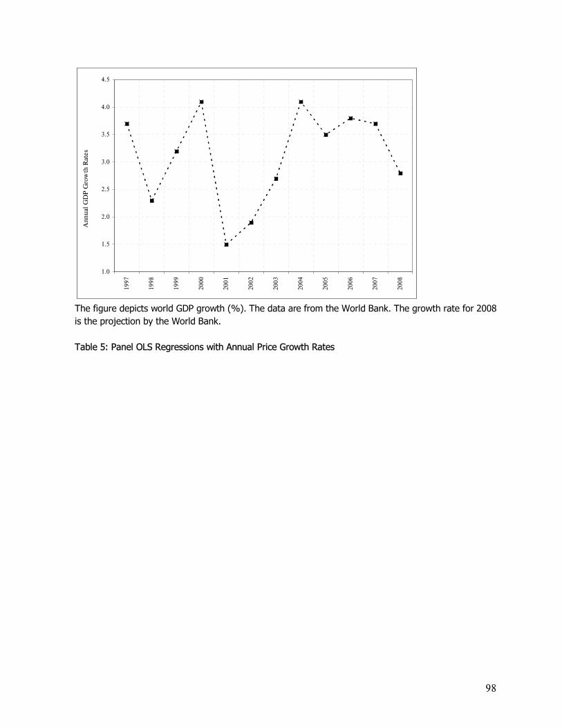
98

1.0

1.5

2.0

2.5

3.0

3.5

4.0

4.5

1997

1998

1999

2000

2001

2002

2003

2004

2005

2006

2007

2008

Ann

ual

GD

P G

row

th R

ates

The figure depicts world GDP growth (%). The data are from the World Bank. The growth rate for 2008 is the projection by the World Bank. Table 5: Panel OLS Regressions with Annual Price Growth Rates

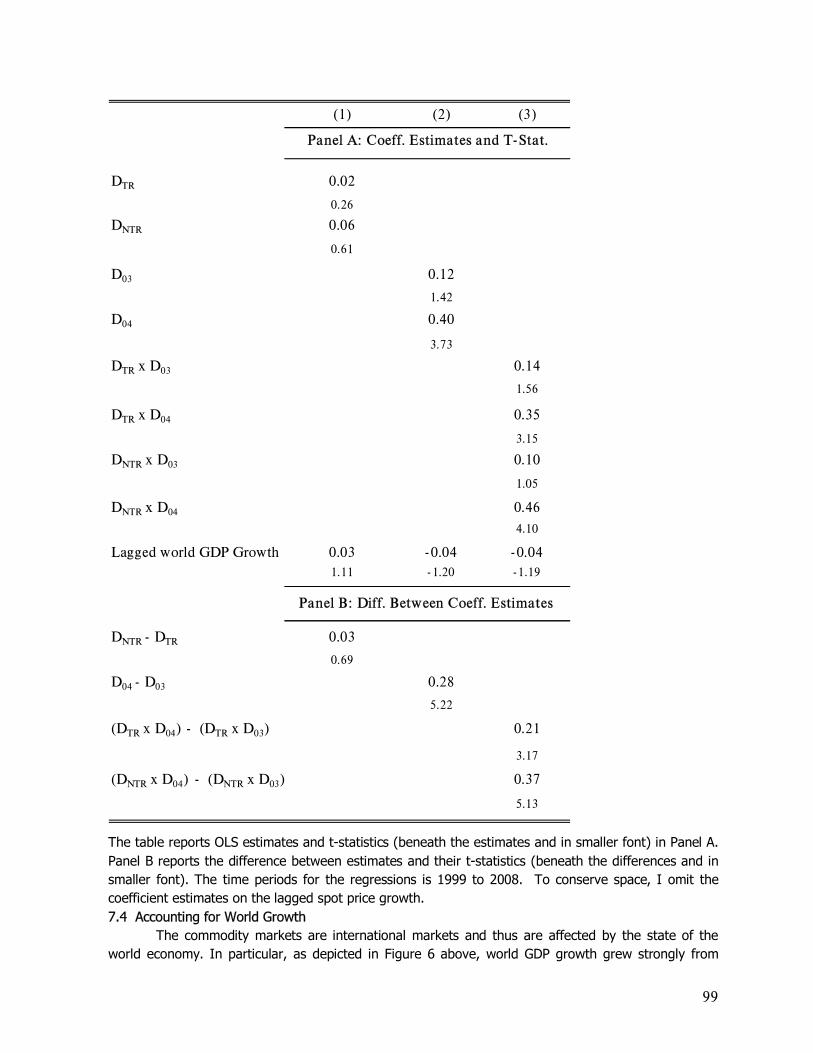
99

(1) (2) (3)

DTR 0.02

0.26

DNTR 0.06

0.61

D03 0.12

1.42

D04 0.40

3.73

DTR x D03 0.14

1.56

DTR x D04 0.35

3.15

DNTR x D03 0.10

1.05

DNTR x D04 0.46

4.10

Lagged world GDP Growth 0.03 - 0.04 - 0.041.11 - 1.20 -1.19

DNTR - DTR 0.03

0.69

D04 - D03 0.28

5.22

(DTR x D04) - (DTR x D03) 0.21

3.17

(DNTR x D04) - (DNTR x D03) 0.37

5.13

Panel A: Coeff. Estimates and T- Stat.

Panel B: Diff. Between Coeff. Estimates

The table reports OLS estimates and t-statistics (beneath the estimates and in smaller font) in Panel A. Panel B reports the difference between estimates and their t-statistics (beneath the differences and in smaller font). The time periods for the regressions is 1999 to 2008. To conserve space, I omit the coefficient estimates on the lagged spot price growth. 7.4 Accounting for World Growth The commodity markets are international markets and thus are affected by the state of the world economy. In particular, as depicted in Figure 6 above, world GDP growth grew strongly from

100

2001 to 2004. The timing of this steady growth in the world economy might explain the increase in the commodity spot price growth rates at 2004. To examine this conjecture, I re-estimate the annual regressions reported in Table 4 (regressions 1 to 3) by including the lag of world GDP growth as an additional control variable. The new regression results are reported in Table 5 and show that accounting for the behavior of world GDP growth cannot explain the structural change at 2004. For example, in the type (c) regression (reported in column 3 of Table 5), the difference between the interaction terms (DTR × D04) and (DTR × D03) is statistically significant (difference = 0.21, t-statistic = 3.17) and it is smaller in magnitude than the difference between (DNTR × D04) and (DNTR × D03) (difference = 0.37, t-statistic = 5.13).

Appendix D. Analysis of exchange-traded commodities We identify 63 commodity ETPs that are invested in commodities or commodity futures. However, institutional holding data is available for only 34 of these ETPs.28 Total 13F institutional holdings are calculated from SEC form 13F by summing all shares held in a given firm across all managers in the quarter. We also calculate the total institutional shares held as a percentage of the firm�s outstanding shares. Institutional holding data is obtained through Thomson Financial based on Form 13F filings submitted to the SEC. The database provides the shares held in a firm for each institution holding shares in a given quarter. Institutions with a portfolio of at least $100 million in U.S. equities are required to report their quarterly positions in those equities to the SEC via Form 13F. Institutions who meet the reporting threshold must report individual holdings of more than 10,000 shares or $200,000 each quarter.29 The analysis here uses June 2008 quarterly filing information. In addition to institutional holdings data, we collect data on the fund�s net assets. Total net assets for the 34 ETPs with available data are $37,663 million. Total net assets for the 29 ETPs without available data are $409 million. Our sample contains four agricultural funds, eleven energy funds, twelve metal funds, and seven mixed commodity funds. In Figure 1, we provide information on total commodity ETP assets over the last year by commodity fund sector and for the SPDR gold shares and iShares silver trust separately. The graph demonstrates that the bulk of investment dollars are allocated to the SPDR Gold Shares and the iShares Silver Trust. In Table 1, we provide basic information on the total assets, level and percentage of institutional holdings by fund. The data show that the number of institutional holders and the percent of shares they own can vary widely across the funds.

28 Many of the ETFs and ETNs with no data have an inception date more recent than December 31, 2007. 29 Our total institutional holdings values for each fund may be downwardly biased due to the lack of reporting for small positions. It is also possible that some individual positions may be over-reported which would upwardly bias our results. There are two possible reasons for this. First, managers who co-manage a portfolio may both report holdings in the single co-managed fund. Second, buyers who transact with short-sellers will report their ownership of the shares, as will as the original owner from which the shares were borrowed.

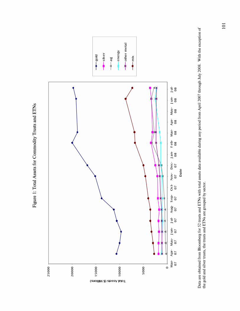
10

1

F

igur

e 1:

Tot

al A

sset

s fo

r C

omm

odit

y T

rust

s an

d E

TN

s

0

50

00

10

000

15

000

20

000

25

000 M

ar-

07

Apr-

07

Ma

y-0

7Ju

n-

07

Ju

l-0

7A

ug

-07

Se

p-

07

Oct-

07

No

v-

07

De

c-

07

Ja

n-

08

Fe

b-

08

Ma

r-0

8A

pr-

08

Ma

y-

08

Ju

n-

08

Ju

l-0

8

Da

te

Total Assets ($ Millions)

go

ld

silv

er

ag

en

erg

y

oth

er

me

tal

mix

D

ata

are

obta

ined

fro

m B

loom

berg

for

52

trus

ts a

nd E

TN

s w

ith t

otal

ass

ets

data

ava

ilabl

e du

ring

any

per

iod

from

Apr

il 20

07 t

hrou

gh J

uly

2008

. W

ith

the

exce

ptio

n of

th

e go

ld a

nd s

ilver

tru

sts,

the

tru

sts

and

ET

Ns

are

grou

ped

by s

ecto

r.

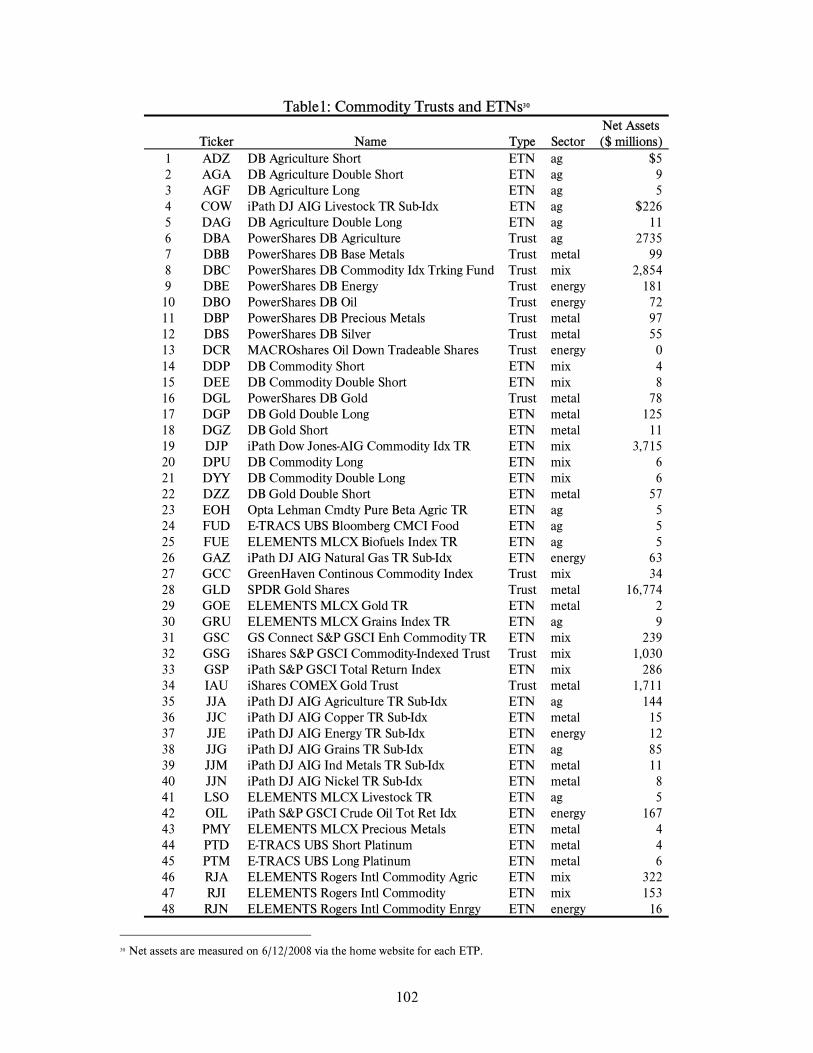
102

Table1: Commodity Trusts and ETNs30

Ticker

Name Type

Sector Net Assets ($ millions)

1 ADZ DB Agriculture Short ETN ag $5 2 AGA DB Agriculture Double Short ETN ag 93 AGF DB Agriculture Long ETN ag 54 COW iPath DJ AIG Livestock TR Sub-Idx ETN ag $226 5 DAG DB Agriculture Double Long ETN ag 116 DBA PowerShares DB Agriculture Trust ag 2735 7 DBB PowerShares DB Base Metals Trust metal 998 DBC PowerShares DB Commodity Idx Trking Fund Trust mix 2,854 9 DBE PowerShares DB Energy Trust energy 181 10 DBO PowerShares DB Oil Trust energy 7211 DBP PowerShares DB Precious Metals Trust metal 9712 DBS PowerShares DB Silver Trust metal 5513 DCR MACROshares Oil Down Tradeable Shares Trust energy 014 DDP DB Commodity Short ETN mix 415 DEE DB Commodity Double Short ETN mix 816 DGL PowerShares DB Gold Trust metal 7817 DGP DB Gold Double Long ETN metal 125 18 DGZ DB Gold Short ETN metal 1119 DJP iPath Dow Jones-AIG Commodity Idx TR ETN mix 3,715 20 DPU DB Commodity Long ETN mix 621 DYY DB Commodity Double Long ETN mix 622 DZZ DB Gold Double Short ETN metal 5723 EOH Opta Lehman Cmdty Pure Beta Agric TR ETN ag 524 FUD E-TRACS UBS Bloomberg CMCI Food ETN ag 525 FUE ELEMENTS MLCX Biofuels Index TR ETN ag 526 GAZ iPath DJ AIG Natural Gas TR Sub-Idx ETN energy 6327 GCC GreenHaven Continous Commodity Index Trust mix 3428 GLD SPDR Gold Shares Trust metal 16,774 29 GOE ELEMENTS MLCX Gold TR ETN metal 230 GRU ELEMENTS MLCX Grains Index TR ETN ag 931 GSC GS Connect S&P GSCI Enh Commodity TR ETN mix 239 32 GSG iShares S&P GSCI Commodity-Indexed Trust Trust mix 1,030 33 GSP iPath S&P GSCI Total Return Index ETN mix 286 34 IAU iShares COMEX Gold Trust Trust metal 1,711 35 JJA iPath DJ AIG Agriculture TR Sub-Idx ETN ag 144 36 JJC iPath DJ AIG Copper TR Sub-Idx ETN metal 1537 JJE iPath DJ AIG Energy TR Sub-Idx ETN energy 1238 JJG iPath DJ AIG Grains TR Sub-Idx ETN ag 8539 JJM iPath DJ AIG Ind Metals TR Sub-Idx ETN metal 1140 JJN iPath DJ AIG Nickel TR Sub-Idx ETN metal 841 LSO ELEMENTS MLCX Livestock TR ETN ag 542 OIL iPath S&P GSCI Crude Oil Tot Ret Idx ETN energy 167 43 PMY ELEMENTS MLCX Precious Metals ETN metal 444 PTD E-TRACS UBS Short Platinum ETN metal 445 PTM E-TRACS UBS Long Platinum ETN metal 646 RJA ELEMENTS Rogers Intl Commodity Agric ETN mix 322 47 RJI ELEMENTS Rogers Intl Commodity ETN mix 153 48 RJN ELEMENTS Rogers Intl Commodity Enrgy ETN energy 16

30 Net assets are measured on 6/12/2008 via the home website for each ETP.

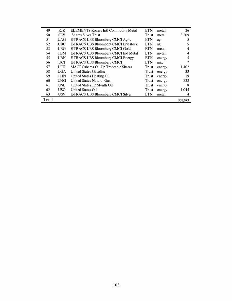
103

49 RJZ ELEMENTS Rogers Intl Commodity Metal ETN metal 2650 SLV iShares Silver Trust Trust metal 3,209 51 UAG E-TRACS UBS Bloomberg CMCI Agric ETN ag 552 UBC E-TRACS UBS Bloomberg CMCI Livestock ETN ag 553 UBG E-TRACS UBS Bloomberg CMCI Gold ETN metal 454 UBM E-TRACS UBS Bloomberg CMCI Ind Metal ETN metal 455 UBN E-TRACS UBS Bloomberg CMCI Energy ETN energy 556 UCI E-TRACS UBS Bloomberg CMCI ETN mix 757 UCR MACROshares Oil Up Tradeable Shares Trust energy 1,402 58 UGA United States Gasoline Trust energy 3359 UHN United States Heating Oil Trust energy 1960 UNG United States Natural Gas Trust energy 823 61 USL United States 12 Month Oil Trust energy 862 USO United States Oil Trust energy 1,045 63 USV E-TRACS UBS Bloomberg CMCI Silver ETN metal 4

Total $38,073

104

105

Glossary of Futures Markets Terms