INTERACTIVE SIMULATION OF AN ULTRASONIC TRANSDUCERAND LASER RANGE SCANNER

By

DAVID NOVICK

A THESIS PRESENTED TO THE GRADUATE SCHOOLOF THE UNIVERSITY OF FLORIDA IN PARTIAL FULFILLMENT

OF THE REQUIREMENTS FOR THE DEGREE OFMASTER OF ENGINEERING

UNIVERSITY OF FLORIDA1993

ii

ACKNOWLEDGEMENTS

The author would like to express his thanks to Dr. Crane.

Using his previous work on object primitives and the graphical

range simulation program allowed the author to concentrate on

improving the original simulation without dedicating time to

develop primitives needed in the simulation. Rob Murphy is to

be acknowledged for his excellent work animating the Kawasaki

Mule 500, used as the navigation test vehicle (NTV).

Thanks go to David Armstrong and Arturo Rankin. David

Armstrong developed the interface between the ultrasonic

sensors and the onboard VME computer. With his help, actual

sonar data, position, and errors were used to accurately

represent sonar in the simulation. Arturo Rankin implemented

the path planning and path execution on the NTV. He used and

tested the simulation of the sonar. From his input,

modifications were made to increase the simulation's

correspondence to the real sensors.

The support of the Department of Energy is acknowledged,

which made it possible to purchase the workstation used in

this thesis.

iii

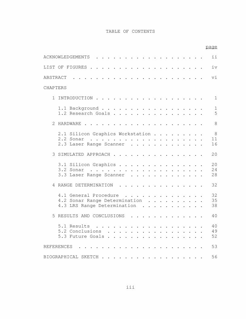
TABLE OF CONTENTS

page

ACKNOWLEDGEMENTS . . . . . . . . . . . . . . . . . . . ii

LIST OF FIGURES . . . . . . . . . . . . . . . . . . . . iv

ABSTRACT . . . . . . . . . . . . . . . . . . . . . . . vi

CHAPTERS

1 INTRODUCTION . . . . . . . . . . . . . . . . . . . 1

1.1 Background . . . . . . . . . . . . . . . . . . 11.2 Research Goals . . . . . . . . . . . . . . . . 5

2 HARDWARE . . . . . . . . . . . . . . . . . . . . . 8

2.1 Silicon Graphics Workstation . . . . . . . . . 82.2 Sonar . . . . . . . . . . . . . . . . . . . . 112.3 Laser Range Scanner . . . . . . . . . . . . . 16

3 SIMULATED APPROACH . . . . . . . . . . . . . . . . 20

3.1 Silicon Graphics . . . . . . . . . . . . . . . 203.2 Sonar . . . . . . . . . . . . . . . . . . . . 243.3 Laser Range Scanner . . . . . . . . . . . . . 28

4 RANGE DETERMINATION . . . . . . . . . . . . . . . 32

4.1 General Procedure . . . . . . . . . . . . . . 324.2 Sonar Range Determination . . . . . . . . . . 354.3 LRS Range Determination . . . . . . . . . . . 38

5 RESULTS AND CONCLUSIONS . . . . . . . . . . . . . 40

5.1 Results . . . . . . . . . . . . . . . . . . . 405.2 Conclusions . . . . . . . . . . . . . . . . . 495.3 Future Goals . . . . . . . . . . . . . . . . . 52

REFERENCES . . . . . . . . . . . . . . . . . . . . . . 53

BIOGRAPHICAL SKETCH . . . . . . . . . . . . . . . . . . 56

iv

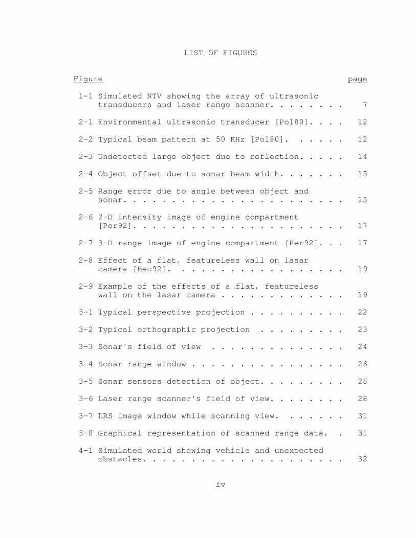
LIST OF FIGURES

Figure page

1-1 Simulated NTV showing the array of ultrasonic transducers and laser range scanner. . . . . . . . 7

2-1 Environmental ultrasonic transducer [Pol80]. . . . 12

2-2 Typical beam pattern at 50 KHz [Pol80]. . . . . . 12

2-3 Undetected large object due to reflection. . . . . 14

2-4 Object offset due to sonar beam width. . . . . . . 15

2-5 Range error due to angle between object and sonar. . . . . . . . . . . . . . . . . . . . . . . 15

2-6 2-D intensity image of engine compartment [Per92]. . . . . . . . . . . . . . . . . . . . . . 17

2-7 3-D range image of engine compartment [Per92]. . . 17

2-8 Effect of a flat, featureless wall on lasar camera [Bec92]. . . . . . . . . . . . . . . . . . 19

2-9 Example of the effects of a flat, featureless wall on the lasar camera . . . . . . . . . . . . . 19

3-1 Typical perspective projection . . . . . . . . . . 22

3-2 Typical orthographic projection . . . . . . . . . 23

3-3 Sonar's field of view . . . . . . . . . . . . . . 24

3-4 Sonar range window . . . . . . . . . . . . . . . . 26

3-5 Sonar sensors detection of object. . . . . . . . . 28

3-6 Laser range scanner's field of view. . . . . . . . 28

3-7 LRS image window while scanning view. . . . . . . 31

3-8 Graphical representation of scanned range data. . 31

4-1 Simulated world showing vehicle and unexpected obstacles. . . . . . . . . . . . . . . . . . . . . 32

v

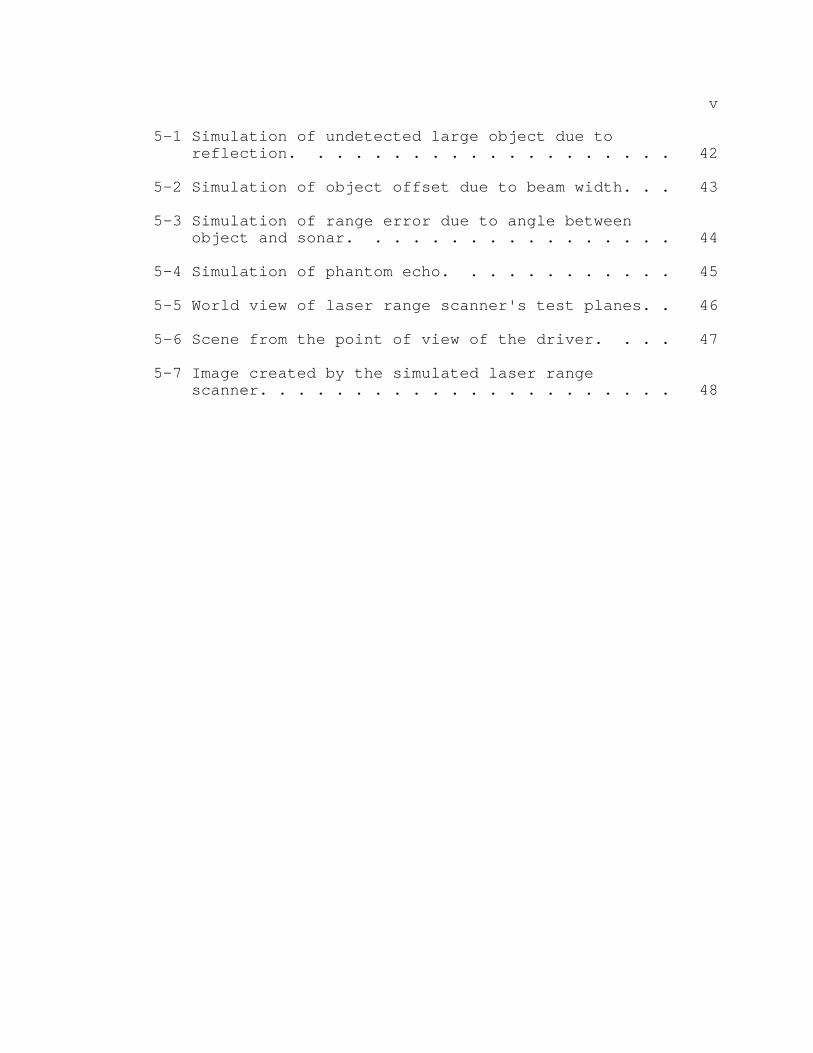
5-1 Simulation of undetected large object due to reflection. . . . . . . . . . . . . . . . . . . . 42

5-2 Simulation of object offset due to beam width. . . 43

5-3 Simulation of range error due to angle between object and sonar. . . . . . . . . . . . . . . . . 44

5-4 Simulation of phantom echo. . . . . . . . . . . . 45

5-5 World view of laser range scanner's test planes. . 46

5-6 Scene from the point of view of the driver. . . . 47

5-7 Image created by the simulated laser range scanner. . . . . . . . . . . . . . . . . . . . . . 48

vi

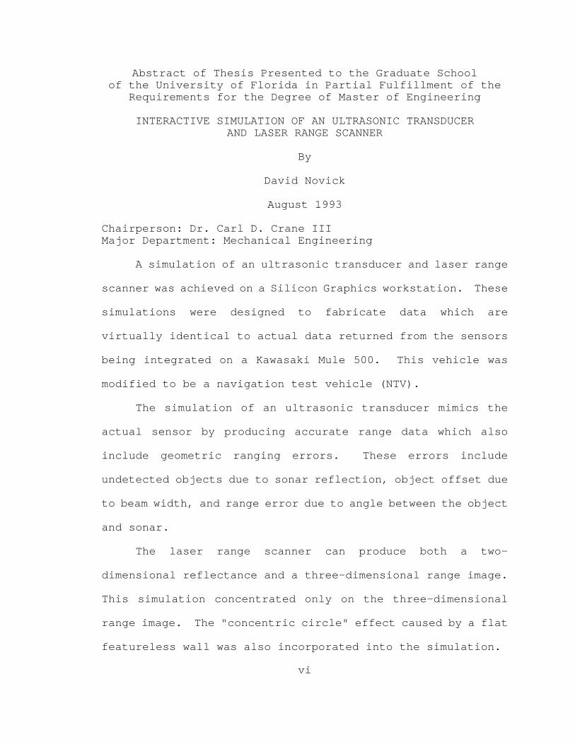
Abstract of Thesis Presented to the Graduate Schoolof the University of Florida in Partial Fulfillment of the

Requirements for the Degree of Master of Engineering

INTERACTIVE SIMULATION OF AN ULTRASONIC TRANSDUCERAND LASER RANGE SCANNER

By

David Novick

August 1993

Chairperson: Dr. Carl D. Crane IIIMajor Department: Mechanical Engineering

A simulation of an ultrasonic transducer and laser range

scanner was achieved on a Silicon Graphics workstation. These

simulations were designed to fabricate data which are

virtually identical to actual data returned from the sensors

being integrated on a Kawasaki Mule 500. This vehicle was

modified to be a navigation test vehicle (NTV).

The simulation of an ultrasonic transducer mimics the

actual sensor by producing accurate range data which also

include geometric ranging errors. These errors include

undetected objects due to sonar reflection, object offset due

to beam width, and range error due to angle between the object

and sonar.

The laser range scanner can produce both a two-

dimensional reflectance and a three-dimensional range image.

This simulation concentrated only on the three-dimensional

range image. The "concentric circle" effect caused by a flat

featureless wall was also incorporated into the simulation.

1

CHAPTER 1INTRODUCTION

1.1 BackgroundSimulation

The human brain has tremendous computational power

dedicated to the processing and integration of sensory input.

Since the early 1970s computer generated graphic displays have

made the job of interpreting a vast amount of data

considerably less difficult. Numbers can be overwhelming, it

is much easier to see changes in data if it is displayed in

graphical terms. Flight-test engineers for the U.S. Air Force

view graphical distributions of the collected data from the

prototype aircraft to evaluate the performance of the aircraft

[Bro89].

Visualization environments, or virtual reality, take

advantage of the brain's capability to process visual data.

NASA's virtual model provides computer-simulated environments

in which users can see, hear, and feel the virtual world.

Users can enter the "world" and move around in it, interacting

within it naturally [Gri91]. Researchers at the Biorobotics

Laboratory of McGill University are building a robot, known as

Micro Surgery Robot 1 (MSR1), that will perform delicate

operations under the control of a human surgeon. The computer

will also create a three-dimensional robot's eye view of the

inside of the eye that the surgeon can see by wearing a

2

virtual reality helmet that has a small screen in front of

each eye [San92].

Examining a simulation of an accident or a catastrophe

can be more beneficial than studying the real incident.

Parameters can be changed to view different outcomes.

Hypercube Simulation Laboratory at the Jet Propulsion

Laboratory has developed a program to simulate a nuclear

attack and a Strategic Defense Initiative. They can also

simulate neural networks, chemical reaction dynamics, and

seismic phenomena [Cul89]. Programming third-generation robot

systems is very difficult because of the need to program

sensor feedback data. A visualization of the sensor view of

a scene, especially the view of a camera, can help the human

planner to improve the programming and verification of an

action plan of a robot. J. Raczkowsky and K. H. Mittenbuehler

simulated a camera for use in robot applications. Their

approach shows the physical modeling, based on a geometric

model of the camera, the light sources, and the objects within

the scene [Rac89].

Improved graphical performance in computer hardware at

reduced costs is leading to the development of interactive

computer graphics and real-time simulations, allowing the

engineer to interact with the simulation. This substantially

boosts productivity for such tasks as visualizing aerodynamic

flow patterns, surface geometry, structural stress and

3

deformation, or other complex physical phenomena. By

observing the results of supercomputations in near real time,

analysts can react quickly to change parameters and make new

discoveries or interpretations [Tho88]. Behavioral animation

is a means for automatic motion control in which animated

objects are capable of sensing their environment and

determining their motion within it according to certain rules.

Jane Wilhelms and Robert Skinner used an interactive method of

behavioral animation in which the user controls motion by

designing a network mapping sensor information to effectors

[Wil90]. Robert E. Parkin developed a graphics package called

RoboSim. RoboSim is intended for the real-time simulation of

the kinematics of automated workcells containing one or more

robots with any configuration and up to six degrees of freedom

[Par91].

Sensors used on Mobile Robots

Robots require a wide range of sensors to obtain

information about the world around them. These sensors detect

position, velocity, acceleration, and range to objects in the

robots workspace. There are many different sensors used to

detect the range to an object. J. C. Whitehouse proposed a

method of rangefinding by measuring the profile of blurs in or

near the back focal plane of a lens or lens system resulting

from the capture of light from a point or line source situated

on an object in the scene [Whi89]. One of the most common

rangefinders is the ultrasonic transducer. Vision systems are

4

also used to greatly improve the robot's versatility, speed,

and accuracy for its complex tasks.

For many experimental automated guided vehicles (AGV),

ultrasonic transducers, or sonar, is frequently used as a

primary means of detecting the boundaries within which the

vehicle must operate. W. S. H. Munro, S. Pomeroy, M. Rafiq,

H. R. Williams, M. D. Wybrow and C. Wykes developed a vehicle

guidance system using ultrasonic sensing. The ultrasonic unit

is based on electrostatic transducers and comprises a separate

linear array and curved divergent transmitter which gives it

an effective field of view of 60N and a range of more than 5

meters [Mun89]. J. P. Huissoon and D. M. Moziar overcame the

limited field of view of a typical sonar sensor by creating a

cylindrical transducer which employs 32 elements distributed

over 120N [Hui89]. By using three speakers fixed in space,

Tatsuo Arai and Eiji Nakano were able to determine the

location of a mobile robot [Ara83]. Finally, Keinosuke Nagai

and James F. Greenleaf use the Doppler effect of a linearly

moving transducer to produce an ultrasonic image [Nag90].

Vision systems provide information that is difficult or

impossible to obtain in other ways. They are designed to

answer one or more basic questions: where is the object, what

is it's size, what is it, and does it pass inspection. Laser

range scanners provide both two-dimensional reflectance and

three-dimensional range images. Andersen et al. produce a

two-dimensional floor map by integrating knowledge obtained

5

from several range images acquired as the robot moves around

in its attempt to find a path to the goal position [And90].

Similar to Arai and Nakano [Ara83], Nishide, Hanawa and Kondo

use a laser scanning system and three corner cubes to

determine a vehicle's position and orientation [Nis86]. Using

a scanning laser rangefinder, Moring et al. were able to

construct a three-dimensional range image of the robot's

world.

1.2 Research Goals

The goal of this research was to implement an interactive

graphical simulation of an ultrasonic transducer and a laser

range scanner on a Silicon Graphics workstation. Simulations

allow a complete testing of algorithms before having to

download the programs into the robot. These sensors will be

used on the Navigational Test Vehicle (NTV) to detect

obstacles in its environment.

Ultrasonic transducers are used on the NTV to detect and

avoid unexpected obstacles. Using the simulation, the

algorithm can be fine tuned before testing begins on the

actual vehicle.

In the future, a vision system including a camera and

laser range scanner, will be used on the NTV to aid in object

identification. The data from this system will be used to

build a graphical world model.

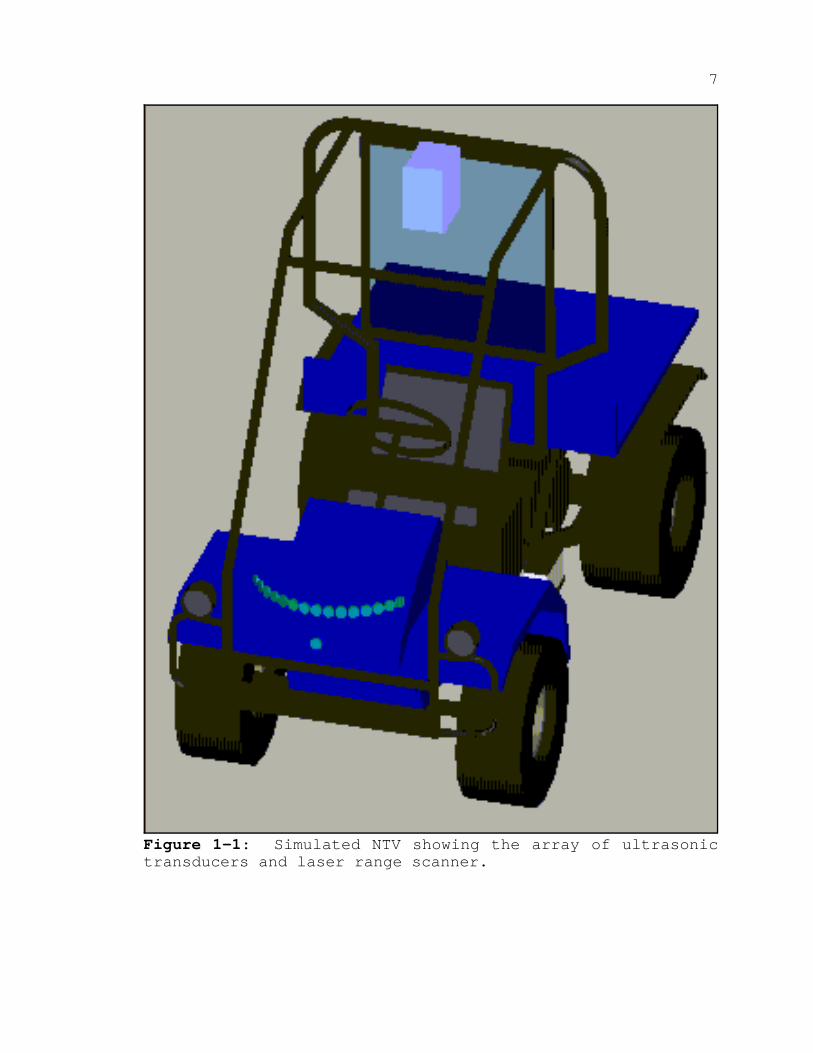
Figure 1-1 shows the NTV and its associated sensors. The

current configuration of the ultrasonic transducers are shown

6

as a small array of circles above the front bumper. The laser

range scanner is the box located directly above the "driver's"

head.

7

Figure 1-1: Simulated NTV showing the array of ultrasonictransducers and laser range scanner.

8

CHAPTER 2HARDWARE

2.1 Silicon Graphics Workstation

The simulation was implemented using a UNIX based Silicon

Graphics IRIS Crimson/VGX workstation. This highperformance

workstation uses a R4000SC superpipelined processor with a 50

MHz external clock (100 MHz internal clock). This R4000SC is

one of a new generation of single-chip RISC processors that

combines the central processing unit (CPU), the floating point

unit (FPU) and cache on one chip. Using this configuration

eliminates the delays that result from passing signals between

chips. The processor provides high resolution 2D and 3D

graphical representations of objects with flicker-free quality

on a 20 inch monitor with 1280 by 1024 resolution [Sil91].

The heart of the system is a pipeline of custom-made,

very large scale integration (VLSI) chips. This pipeline, or

Geometry Engine, performs in hardware such time consuming

operations as matrix multiplication, edge clipping, coordinate

transformation and rotation from a user-defined world

coordinate system to the screen coordinate system. A four by

four matrix multiplication,

an operation done repeatedly in 3D transformations, is

performed rapidly by the pipeline.

Included with the station is Silicon Graphics's Graphics

Library (GL). The GL is a library of subroutine primitives

9

that can be called from a C program (or other language). These

primitives include support for input devices such as the

mouse, keyboard, spaceball, trackball, and digitizing tablet.

From this library a programmer can define object, world, and

viewing coordinate systems and apply orthographic or

perspective projections to map these to any viewport on the

screen. Objects can then be translated, rotated, and scaled

in real time. The library contains two different methods of

displaying colors: color map and RGB mode. There are also two

different methods of displaying graphics: single and double

buffer mode.

The image memory consists of twenty-four 1024 by 2048

bitplanes. Each plane provides one bit of color information

for a maximum display of 224 (16,777,216) colors. In color map

mode, an integer representing a certain color is specified,

and the current color is set to this new color. For example,

GREEN is an index into the color table that sets the current

color to green.

The second method of displaying color is RGB mode. In

this mode, the intensities for the red, green, and blue

electron gun are specified in vector form with values ranging

from 0 to 1. The three vectors [1.0 0.0 0.0], [0.0 1.0 0.0],

and [0.0 0.0 1.0] correspond to a pure red, pure green, and

pure blue respectively.

10

A complicated illustration is composed of many smaller

graphical elements, such as cubes, cylinders, and cones. In

single buffer mode, these elements are displayed on the

screen, one by one, until the scene is completed. While this

method works well for static pictures, it is unsuitable for

animation. If the picture constantly changes, the viewer may

see the retrace of the image leading to a flicker between

frames.

When flicker-free animation is desired, double buffer

mode should be chosen. A scene needs to be displayed at least

12 frames/second (fps) to produce a flicker-free animation.

Movies are displayed at 24 fps. In double buffer mode, the 24

color bitplanes are split into two separate buffers, front and

back, each consisting of 12 color bitplanes. The drawing is

rendered in the back buffer, while the front buffer is

displayed on the screen. When the GL routine swapbuffers() is

called, the buffers are swapped during a video retrace.

Image depth sorting is accomplished using the Z-buffer

technique. An array of memory 1280 by 1024 is initialized

with the maximum depth. Each cell of the memory corresponds

to each pixel on the screen. The image is drawn on a pixel by

pixel basis, and the depth of the current pixel is compared to

the depth of the corresponding memory address. If the pixel

is "closer" to the viewer its color and depth are placed in

11

R 'ct2 Eqn 2-1

c ' ?RT ms Eqn 2-2

c ' 20 T ms Eqn 2-3

the Z-buffer memory. With this technique, complicated images,

such as intersecting polygons, can be drawn rapidly with

little effort to the programmer.

2.2 Sonar

In a sonar ranging system, a short acoustic pulse is

first emitted from a transducer. The transducer then switches

to the receive mode where it waits for a specified amount of

time before switching off (user defined). If a return echo is

detected, the range, R, can be found by multiplying the speed

of sound by one half the time measured. The time is halved

since the time measured includes the time taken to strike the

object, and then return to the receiver.

where c is the speed of sound and t is the time in seconds.

The speed of sound, c, can be found by treating air as an

ideal gas and using the equation

where ? = 1.4, R = 287 m2/(s2K), and the temperature, T, is in

Kelvins. Substituting in the values, the equation reduces to

12

Figure 2-1: Environmental ultrasonic transducer [Pol80].

Figure 2-2: Typical beam pattern at50 KHz [Pol80].

which is valid to within 1% for most conditions. The speed of

sound is thus proportional to the temperature. At room

temperature (20 NC, 68 NF) the values are:

cm = 343.3 m/s, cf = 1126.3 f/s

The sonar array consisted of 16 Polaroid environmental

ultrasonic transducers shown in figure 2-1. They are

instrument grade ultrasonic transducers intended for operation

in air. Figure 2-2

shows the typical beam

pattern at 50 KHz. From

the figure it can been

seen that at 15N from

the centerline of the

sonar, in both

directions, the response

drops off drastically, thus producing a 30N cone. The range

13

is accurate from 6 inches to 35 feet, with a resolution of ±

1%.

The Polaroid transducers are driven by a Transitions

Research Corporation (TRC) subsystem. The controller board

contains a Motorola 68HC11 CPU and serial communications

hardware. Each board can control up to eight ultrasonic

transducers and eight infrared sensors. Additionally, two

more controllers could be integrated for a total of 24

ultrasonic transducers and 24 infrared sensors.

Common to all sonar ranging systems is the problem of

sonar reflection. With light waves, our eye can see objects

because the incident light energy is scattered by most

objects, which means that some energy will reach our eye,

despite the angle of the object to us or to the light source.

This scattering occurs because the roughness of an object's

surface is large compared to the wavelength of light (.550

nm). Only with very smooth surfaces (such as a mirror) does

the reflectivity become highly directional for light rays.

Ultrasonic energy has wavelengths much larger (.0.25 in) in

comparison. Therefor, ultrasonic waves find almost all large

flat surfaces reflective in nature. The amount of energy

returned is strongly dependent on the incident angle of the

sound energy [Poo89]. Figure 2-3 shows a case where a large

object is not detected because the energy is reflected away

from the receiver.

14

Sonar

Reflected Energy

Reflected Energy

LargeObstacle

Figure 2-3: Undetected large objectdue to reflection.

X ' Rsinf

Although the basic range formula is accurate, there are

several factors when considering the accuracy of the result.

Since the speed of sound relies on the temperature, a 10N

temperature difference, may cause the range to be in error by

1%. Geometry also affects range in two major ways. The

range equation assumes that the sonar beam width is

negligible. An object may be off center, but normal to the

transmitted beam. The range computed will be correct, but the

X-component may be in error. Using the formula:

at a range of 9 meters and a beam width of 30N, the X-

component would be 2.33 meters off center. Figure 2-4

illustrates this.

15

BeamWidth

X-Offset

AssumedObject

Position

ActualObject

Position

Sonar

Figure 2-4: Object offset due tosonar beam width.

Actual RangeSonar

Figure 2-5: Range error due to anglebetween object and sonar.

Another geometric effect is shown in figure 2-5. When

the object is at an angle to the receiver, the range computed

will be to the closest point on the object, not the range from

the center line of the beam [Reu91].

16

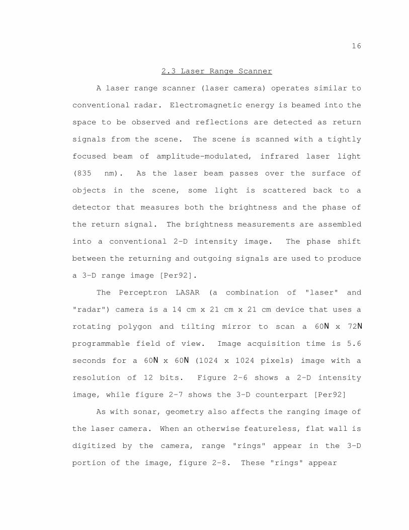
2.3 Laser Range Scanner

A laser range scanner (laser camera) operates similar to

conventional radar. Electromagnetic energy is beamed into the

space to be observed and reflections are detected as return

signals from the scene. The scene is scanned with a tightly

focused beam of amplitude-modulated, infrared laser light

(835 nm). As the laser beam passes over the surface of

objects in the scene, some light is scattered back to a

detector that measures both the brightness and the phase of

the return signal. The brightness measurements are assembled

into a conventional 2-D intensity image. The phase shift

between the returning and outgoing signals are used to produce

a 3-D range image [Per92].

The Perceptron LASAR (a combination of "laser" and

"radar") camera is a 14 cm x 21 cm x 21 cm device that uses a

rotating polygon and tilting mirror to scan a 60N x 72N

programmable field of view. Image acquisition time is 5.6

seconds for a 60N x 60N (1024 x 1024 pixels) image with a

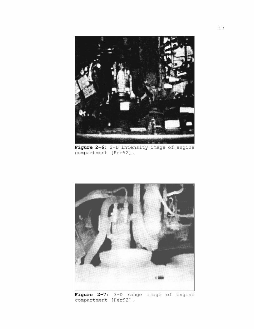
resolution of 12 bits. Figure 2-6 shows a 2-D intensity

image, while figure 2-7 shows the 3-D counterpart [Per92]

As with sonar, geometry also affects the ranging image of

the laser camera. When an otherwise featureless, flat wall is

digitized by the camera, range "rings" appear in the 3-D

portion of the image, figure 2-8. These "rings" appear

17

Figure 2-6: 2-D intensity image of enginecompartment [Per92].

Figure 2-7: 3-D range image of enginecompartment [Per92].

18

because of the rotating polygon and tilting mirror used to

generate the raster scan of the scene. Since the shortest

distance to the wall is perpendicular, as the laser beam that

is directed by the tilting mirror moves off from the

perpendicular the measured distance to the wall increases. At

30N the apparent distance has increased by 15.5%. The "rings"

or steps in range then emerge because of the resolution of the

camera (12 bits). When the measured range increases by one

step in resolution, the distance calculated for the pixel

corresponding to the associated range data is greater. The

pixel associated with that scan becomes a shade darker. For

example, see figure 2-9, at a maximum range of 40 meters, the

resolution is 1 cm. If a flat wall was 20 meters from the

scanner, at 17.7N from the normal, a perceived change in

distance would occur.

19

Figure 2-8: Effect of a flat,featureless wall on lasar camera[Bec92].

LRS

17.7°

Figure 2-9: Example of the effects of aflat, featureless wall on the lasar camera

20

CHAPTER 3SIMULATED APPROACH

3.1 Silicon Graphics

The three major routines of the GL used in the simulation

were z-buffer, feedback, and projection transformations. Z-

buffer provided the depth sorting, while feedback provided the

data needed to perform the necessary calculations of distance

and normal vectors of planes. The projection transformations

define which objects can be seen, and how they are portrayed

within the viewing volume.

When displaying graphics, the calls to the GL send a

series of commands and data down the Geometry Pipeline. The

pipeline transforms, clips, and scales the data. Lighting

calculations are done and colors computed. The points, lines,

and polygons are then scan-converted and the appropriate

pixels in the bitplanes are set to the proper values.

A call to feedback places the system into feedback mode.

Feedback is a system-dependent mechanism in the form:

count=feedback(array_name,size_of_array)

The GL commands send exactly the same information into the

front of the pipeline, but the pipeline is short-circuited.

The Geometry Engine is used in feedback to transform, clip,

and scale vertices to screen coordinates, and to do the basic

lighting calculations. This raw output is then returned to

the host process in the form of an array, array_name. The

21

number of elements stored in the array is returned by the

feedback routine, count.

The information returned in the array is in the following

format:

<data type> <count> <count words of data>

There are five data types: FB_POINT, FB_LINE, FB_POLYGON,

FB_CMOV, and FB_PASSTHROUGH. The actual values of these data

types are defined in gl/feed.h. The formats are as follows:

FB_POINT, count (9.0), x, y, z, r, g, b, a, s, t.

FB_LINE, count (18.0), x1, y1, z1, r1, g1, b1, a1, s1,

t1, x2, y2, z2, r2, g2, b2, a2, s2, t2.

FB_POLYGON, count (27.0), x1, y1, z1, r1, g1, b1, a1, s1,

t1, x2, y2, z2, r2, g2, b2, a2, s2, t2, x3, y3, z3, r3,

g3, b3, a3, s3, t3.

FB_PASSTHROUGH, count (1.0), passthrough.

FB_CMOV, count (3.0), x, y, z.

The x and y values are in floating point screen coordinates,

the z value is the floating point transformed z. Red (r),

green (g), blue (b), and alpha (a) are floating point values

ranging from 0.0 to 255.0, which specify the RGB values of the

point and its transparency. The s and t values are floating

point texture coordinates [Sil91].

To move from the world coordinate system, where all the

objects in the scene are defined, to the screen coordinate

system, the scene you see on the screen, a projection

22

Figure 3-1: Typical perspectiveprojection

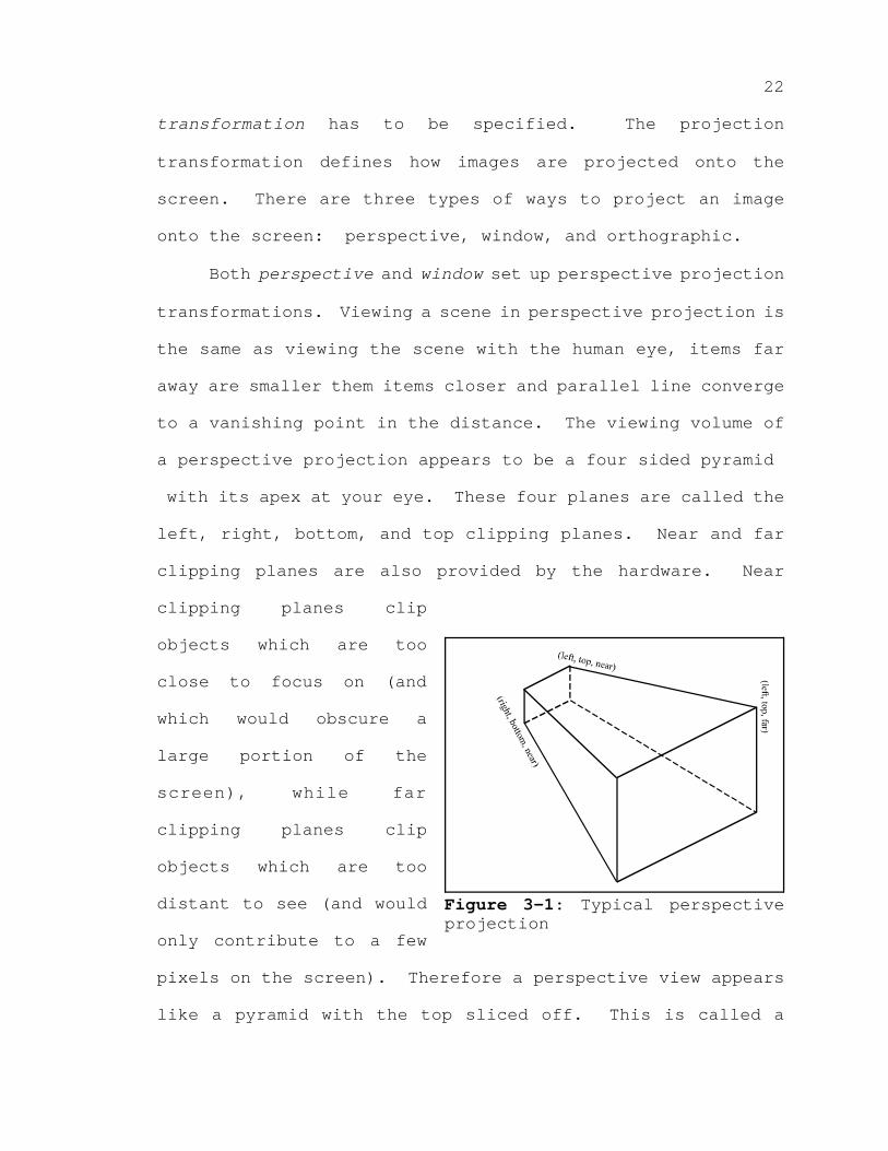
transformation has to be specified. The projection

transformation defines how images are projected onto the

screen. There are three types of ways to project an image

onto the screen: perspective, window, and orthographic.

Both perspective and window set up perspective projection

transformations. Viewing a scene in perspective projection is

the same as viewing the scene with the human eye, items far

away are smaller them items closer and parallel line converge

to a vanishing point in the distance. The viewing volume of

a perspective projection appears to be a four sided pyramid

with its apex at your eye. These four planes are called the

left, right, bottom, and top clipping planes. Near and far

clipping planes are also provided by the hardware. Near

clipping planes clip

objects which are too

close to focus on (and

which would obscure a

large portion of the

screen), while far

clipping planes clip

objects which are too

distant to see (and would

only contribute to a few

pixels on the screen). Therefore a perspective view appears

like a pyramid with the top sliced off. This is called a

23

(left, top, near)

(right, bottom, far)

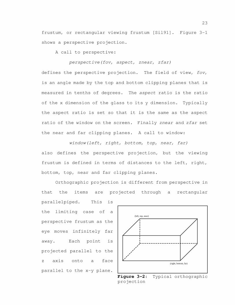
Figure 3-2: Typical orthographicprojection

frustum, or rectangular viewing frustum [Sil91]. Figure 3-1

shows a perspective projection.

A call to perspective:

perspective(fov, aspect, znear, zfar)

defines the perspective projection. The field of view, fov,

is an angle made by the top and bottom clipping planes that is

measured in tenths of degrees. The aspect ratio is the ratio

of the x dimension of the glass to its y dimension. Typically

the aspect ratio is set so that it is the same as the aspect

ratio of the window on the screen. Finally znear and zfar set

the near and far clipping planes. A call to window:

window(left, right, bottom, top, near, far)

also defines the perspective projection, but the viewing

frustum is defined in terms of distances to the left, right,

bottom, top, near and far clipping planes.

Orthographic projection is different from perspective in

that the items are projected through a rectangular

parallelpiped. This is

the limiting case of a

perspective frustum as the

eye moves infinitely far

away. Each point is

projected parallel to the

z axis onto a face

parallel to the x-y plane.

24

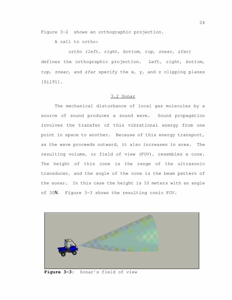
Figure 3-3: Sonar's field of view

Figure 3-2 shows an orthographic projection.

A call to ortho:

ortho (left, right, bottom, top, znear, zfar)

defines the orthographic projection. Left, right, bottom,

top, znear, and zfar specify the x, y, and z clipping planes

[Sil91].

3.2 Sonar

The mechanical disturbance of local gas molecules by a

source of sound produces a sound wave. Sound propagation

involves the transfer of this vibrational energy from one

point in space to another. Because of this energy transport,

as the wave proceeds outward, it also increases in area. The

resulting volume, or field of view (FOV), resembles a cone.

The height of this cone is the range of the ultrasonic

transducer, and the angle of the cone is the beam pattern of

the sonar. In this case the height is 10 meters with an angle

of 30N. Figure 3-3 shows the resulting conic FOV.

25

Since there is no conic viewing volume, a perspective

projection was used to simulate the sonar's conic FOV. Using

min=0.05(m), p_size=min*TAN15(m) and the call window (-p_size,

p_size, -p_size, p_size, min, MAX_SONAR_DIST) a perspective

volume with the minimum distance set to 0.05 meters and the

maximum distance set to MAX_SONAR_DIST was created.

There are certain options a user can utilize to

initialize the simulation, some of them are pre-processor

definitions, while others are global variables.

The pre-processor definitions include:

MAX_SONAR_DIST - Maximum range of the ultrasonic transducer.

NUM_SONAR - Number of operating sonar sensors on the vehicle.Each sonar is drawn such that the z-axis points outof the sonar.

The global variables include:

sonar_pos[] - Vector defining the x, y, and z position in thevehicle coordinate system of each ultrasonictransducer. Defined to be of size NUM_SONAR.

sonar_ang[] - Defines the angle of each sonar in the xy planeof the vehicle coordinate system. Defined to be ofsize NUM_SONAR.

sonar_dist[] - Range data calculated for each sonar. Defined to be of size NUM_SONAR.

There are three routines that were written as part of the

sonar simulation: sonar_window_open, Sonar, and draw_sonar.

These are used to initialize the small sonar window, calculate

the range values, and draw the ultrasonic transducers and

their respective FOV cones. Before any of these can be

called, a font and its corresponding size must be chosen.

26

Figure 3-4: Sonar rangewindow

Sonar_window_open needs only to be called once in the

beginning of the main program. It is in the form:

window_id=sonar_window_open(x1,x2,y1,y2,fnsize)

The first four of the five parameters are the coordinates of

the small sonar window starting from bottom left corner to

upper right corner. This routine returns the window

identification number of the window opened. Inside the

routine the sonar window is set up according to the user

specified parameters, the number of ultrasonic transducers and

the size of the font used. The non-varying text is drawn in

yellow. Finally a screenmask is created to mask off non-

varying text area, increasing

window refresh speed. Figure 3-4

show the widow created. Green

numbers represent sonar sensors

which received no return echoes,

and are set to 10 meters. Red

numbers represent the range to

the object returning an echo.

The routine called to

determine the range values of

each ultrasonic transducer is

Sonar in the form:

Sonar(veh_x, veh_y, veh_gam)

Veh_x and veh_y are the

coordinates of the mobile vehicle measured from the world

27

coordinate system. Veh_gam is the orientation of the vehicle

measured from the world X axis. The subroutine draws the

scene from the perspective of each of the ultrasonic

transducers and checks for any object within the viewing

volume. If an object is within the viewing volume the angle

between the object and the sensor is computed to determine if

a return echo is detected. Finally the range values for each

sonar are stored in the global array sonar_dist[].

The final routine which needs to be called after Sonar is

draw_sonar. It's parameters are in the same form as Sonar:

draw_sonar(veh_x, veh_y, veh_gam)

Using the global arrays sonar_pos[] and sonar_ang[], the sonar

hardware is drawn. The color of the sonar cone is determined

by the range reported by the global array sonar_dist[]. If

the range is equal to MAX_SONAR_DIST, a green cone is drawn,

otherwise a red cone is scaled to the range and drawn.

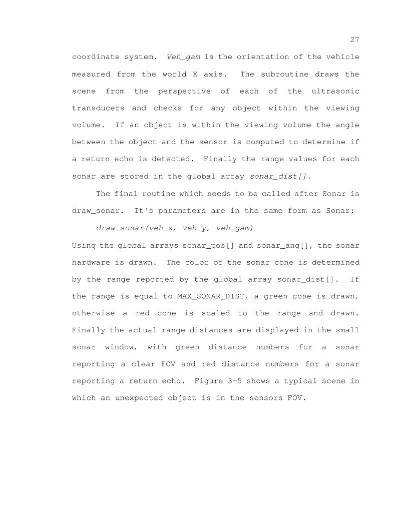
Finally the actual range distances are displayed in the small

sonar window, with green distance numbers for a sonar

reporting a clear FOV and red distance numbers for a sonar

reporting a return echo. Figure 3-5 shows a typical scene in

which an unexpected object is in the sensors FOV.

28

Figure 3-5: Sonar sensors detectionof object.

Figure 3-6: Laser range scanner'sfield of view.

3.3 Laser Range Scanner

The laser range scanner (LRS) uses a single, tightly

focused beam of coherent light to determine the 2D reflection

and 3D range information from a scanned scene. The resulting

FOV is a cylinder, whose height indicates the range of the

beam, and whose diameter indicates the width of the beam.

29

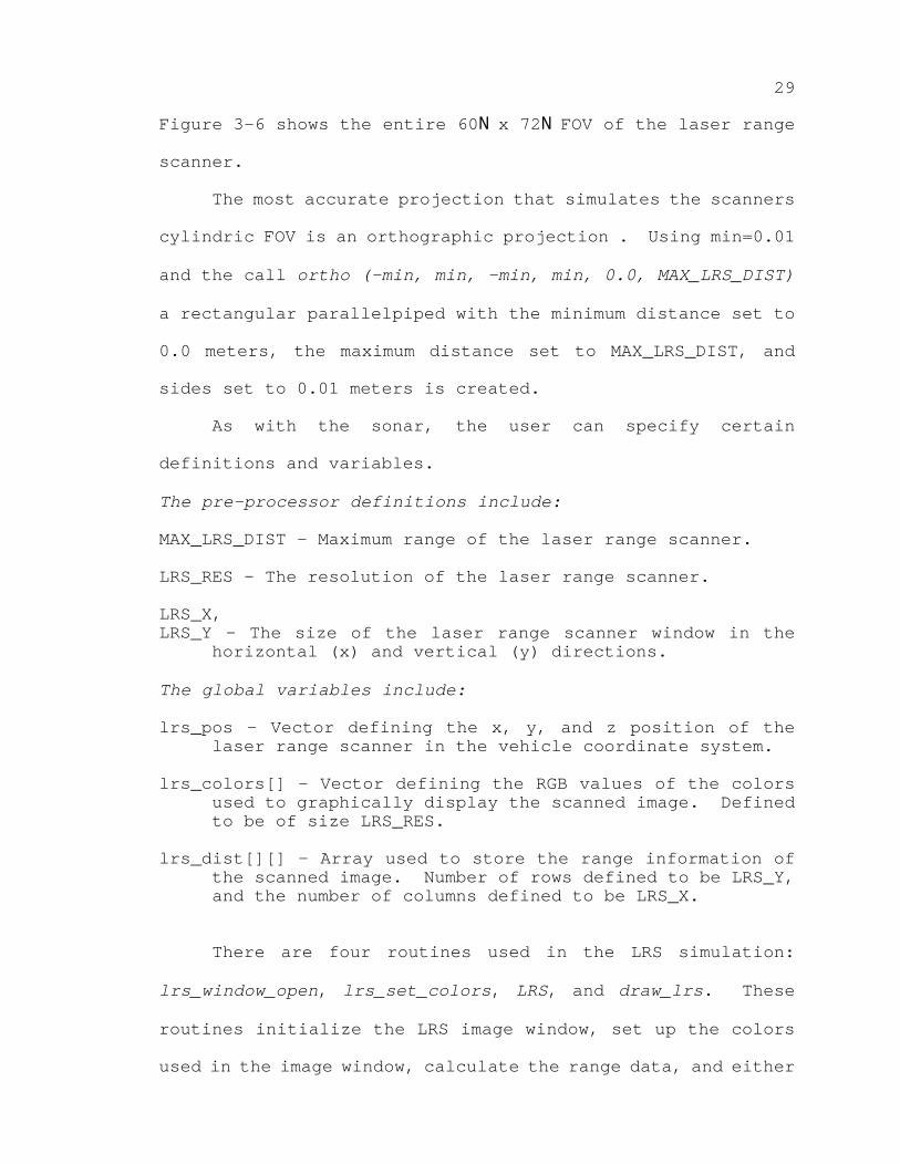
Figure 3-6 shows the entire 60N x 72N FOV of the laser range

scanner.

The most accurate projection that simulates the scanners

cylindric FOV is an orthographic projection . Using min=0.01

and the call ortho (-min, min, -min, min, 0.0, MAX_LRS_DIST)

a rectangular parallelpiped with the minimum distance set to

0.0 meters, the maximum distance set to MAX_LRS_DIST, and

sides set to 0.01 meters is created.

As with the sonar, the user can specify certain

definitions and variables.

The pre-processor definitions include:

MAX_LRS_DIST - Maximum range of the laser range scanner.

LRS_RES - The resolution of the laser range scanner.

LRS_X,LRS_Y - The size of the laser range scanner window in the

horizontal (x) and vertical (y) directions.

The global variables include:

lrs_pos - Vector defining the x, y, and z position of thelaser range scanner in the vehicle coordinate system.

lrs_colors[] - Vector defining the RGB values of the colorsused to graphically display the scanned image. Definedto be of size LRS_RES.

lrs_dist[][] - Array used to store the range information ofthe scanned image. Number of rows defined to be LRS_Y,and the number of columns defined to be LRS_X.

There are four routines used in the LRS simulation:

lrs_window_open, lrs_set_colors, LRS, and draw_lrs. These

routines initialize the LRS image window, set up the colors

used in the image window, calculate the range data, and either

30

draw the LRS FOV in the large window or the scanned image in

the LRS image window. As in the sonar simulation, a font and

its corresponding size must also be chosen.

Lrs_window_open only needs to be called once in the

beginning of the main program. It is in the form:

window_id=lrs_window_open(x1,x2,y1,y2,fnsize)

The first four parameters specify the size and location of the

LRS image window, while the last parameter specifies the font

size used. Upon conclusion, the routine returns the window

identification number. This routine creates the LRS image

window specified by the user and the user defined parameters.

Lrs_set_colors is called and a scale is placed along the right

hand side showing the minimum to maximum distance

(MAX_LRS_DIST) and the corresponding color scale. A

screenmask is used to mask off this scale.

Lrs_set_colors does not use any parameters. It is used

to set the global variable lrs_colors. The colors are in gray

scale and range from white at a distance of 0 meters to black

at a distance of MAX_LRS_DIST.

LRS is called when a scanned image of the scene is

desired. The parameters used are veh_x, veh_y, veh_gam in the

form:

LRS(veh_x, veh_y, veh_gam)

The scene is redrawn LRS_X * LRS_Y times in the perspective of

each point on the LRS image window. The scan starts in the

bottom left and moves across horizontally, then moves

31

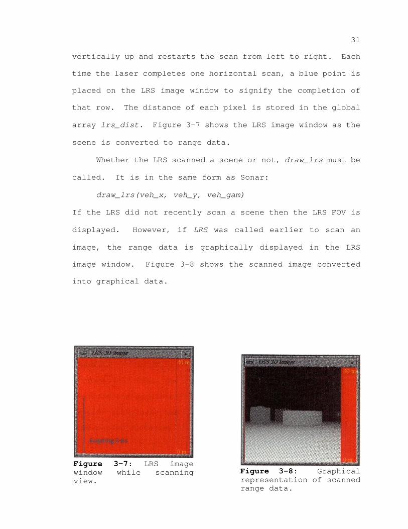
Figure 3-8: Graphicalrepresentation of scannedrange data.

Figure 3-7: LRS imagewindow while scanningview.

vertically up and restarts the scan from left to right. Each

time the laser completes one horizontal scan, a blue point is

placed on the LRS image window to signify the completion of

that row. The distance of each pixel is stored in the global

array lrs_dist. Figure 3-7 shows the LRS image window as the

scene is converted to range data.

Whether the LRS scanned a scene or not, draw_lrs must be

called. It is in the same form as Sonar:

draw_lrs(veh_x, veh_y, veh_gam)

If the LRS did not recently scan a scene then the LRS FOV is

displayed. However, if LRS was called earlier to scan an

image, the range data is graphically displayed in the LRS

image window. Figure 3-8 shows the scanned image converted

into graphical data.

32

Figure 4-1: Simulated world showingvehicle and unexpected obstacles.

CHAPTER 4RANGE DETERMINATION

4.1 General Procedure

In the simulation, the position and orientation of the

mobile vehicle as well as the location of all objects are

known in the world coordinate system. The locations of the

unexpected obstacles are known by the simulation programmer,

but not by the navigation algorithm which is being tested and

developed. The feedback ranging technique is then applied by

drawing the scene from the vantage point of the sensor. The

scene is drawn in feedback buffer mode and the feedback data

buffer is then parsed to determine the distance to the nearest

obstacle. Figure 4-1 shows the vehicle and simulated world

with all the unexpected obstacles.

To draw the

unexpected obstacles

from the point of view

of the sensor, the

coordinate system must

be modified through

translations and

rotations until it is

aligned with the world

coordinate system.

Once this is done, the

33

unexpected obstacles can be drawn since they are defined in

terms of the world coordinate system. Any object intersecting

the viewing volume will be placed into the feedback data

buffer, and its range from the sensor can then be calculated.

The first modification to the coordinate system involves

aligning it with the vehicle coordinate system. This is

accomplished via the following three rotations and one

translation:

rotate(-900, 'x') ;rotate( 900, 'z') ;rot (-sen_ang, 'z') ;

translate (-sen_x, -sen_y, -sen_z) ;

The first rotation is necessary since the original coordinate

system is aligned such that the x-axis lies horizontally, the

y-axis lies vertically, and the z-axis points out of the

screen. The second rotation aligns the x-axis with the

sensor's x-axis. The final rotation aligns the x and y axis

with the vehicle's coordinate system. The final step

translates the coordinate system from the sensor position to

the vehicle's axis. In the section of code shown above two

different rotations routines are listed, rotate and rot.

While they both accomplish the same objective, they use

different parameters. Rotate uses a integer value in tenths

of a degree to specify the rotation about the axis, whereas

rot uses a floating point value to indicate the degree of

rotation. For example, a 43.2N rotation about the y-axis,

rotate (432, 'y') would be used for the integer version, and

34

rot (43.2, 'y') would be used for the floating point version.

The final modification of the coordinate system aligns it with

the world coordinate system:

rot (-veh_ang, 'z') ;translate (-veh_x, -veh_y, -veh_z) ;

These four rotations and two translations define a 4x4

transformation matrix. This matrix will transform points in

the world coordinate system into points in the sensor

coordinate system.

To calculate the range to the obstacle, the Z-buffer is

turned on and the workstation is placed in feedback mode. The

unexpected obstacles are drawn and feedback mode is turned

off.

short feedbuf[1000] ;...

lsetdepth(0, getgdesc(GD_ZMAX)) ;zbuffer(TRUE) ;

feedback(feedbuf, 200); draw_unexpected_obstacles() ;count=endfeedback(feedbuf) ;

The lsetdepth command sets the Z-buffer bit planes to range

from 0 to getgdesc(GD_ZMAX), or on this hardware, from 0 to

8,388,607. If count is greater then zero, then objects from

the simulated world were drawn in the sensor's viewing volume.

Finally the array, feedbuf, is parsed to determine the closest

object. Since all the graphical primitives are drawn with

polygons, the only data type scrutinized is FB_POLYGON, all

other types are disregarded. To obtain the distance from the

35

sensor to the object, the three z values from the FB_POLYGON

data type are averaged, and converted to a "real world"

distance. Since the z values stored in feedbuf are floating

point transformed z values ranging from 0 to 8,388,607, it is

necessary to multiply the values with the ratio

(MAX_SENSOR_DIST/getgdesc(GD_ZMAX)). This converts the

transformed z values into ranges from 0 to MAX_SENSOR_DIST.

4.2 Sonar Range Determination

To determine if a sonar sensor receives a return echo,

and the resulting distance to the object, two passes are

required. From these two passes the range and angle between

the sensor and object are determined.

In the first pass, the unexpected obstacles are passed

through a 4x4 transformation which maps the points into a

perspective projection from the point of view of the sensor.

Since a perspective projection physically alters the objects,

the distance and angle can not be accurately determined. The

first pass is only used to detect the presence of any

unexpected obstacles within the viewing volume of the sensor.

Once it has been determined that there are unexpected

obstacles within the range of the sensor, a second pass is

used to calculate the range and angle of the closest one. An

orthographic projection is used so that the objects are not

altered by the viewing volume. Five different regions of the

sonar's FOV are used to accurately determine if the reflection

from the object is sensed by the sonar. The five different

36

projections correspond to the upper left, upper right, center,

lower left, and lower right portions of the sonar's FOV. Each

orthographic projection is stored in an Object data type,

ortho_p, using makeobj(object) and closeobj(). Makeobj

creates and names a new object by entering the identifier,

specified by object, into a symbol table and allocating memory

for its list of drawing routines. Drawing routines are then

added into the display list until closeobj is called. The

projection is then called using callobj(object).

Once feedbuf has been filled with data from the

unexpected objects, it is necessary to parse through the array

to find the nearest one. From the FB_POLYGON data type, three

points on the plane are stored. Using the z values, the

distance from the sensor to the objects is found, using

(MAX_SONAR_DIST/getgdesc(GD_ZMAX)), and stored in dist1,

dist2, dist3. The average of the three distances is used as

the range to the object. To find the angle between the object

and the sonar, the normal of the plane must be found. Then by

using the dot product, the angle between the normal of the

plane and the sonar vector can be found. To determine the

normal to the plane, the three sets of x and y points, which

are in screen coordinates, must be converted to points that

lie on the plane.

The first step in finding the normal of the plane uses

mapw. Mapw is in the form:

37

mapw(object, x, y, &wx1, &wy1, &wz1, &wx2, &wy2, &wz2)

Object is the object type used to draw the scene and in this

case is ortho_p. The next two parameters, x and y, are the x

and y screen coordinates provided by the feedback data type.

Normally, points in the world coordinate system are

transformed into screen coordinates. By using a backward

transformation, screen coordinates can be transformed into a

line in space. The routine returns two points on the line

designated by the x and y screen coordinates. These two

points are returned in the (wx1, wy1, wz1) and (wx2, wy2, wz2)

parameters respectively. The second step involves converting

the two points on the line into the equation of the line, and

from there into three points on the plane.

Knowing two points on a line it is an easy matter to

convert these into a 3 space paramatized line equation in the

form:

x = x0 + a*ty = y0 + b*tz = z0 + c*t

where a, b, c are the vector components in the form ai+bj+ck

and t is the parameter. By replacing x0, y0, and z0 with the

three sets of initial points wx1, wy1, and wz1, and using the

three different distances, dist1, dist2, and dist3, three

points which lie on the plane are found. The final step in

finding the normal is to create two vectors, one from the

first to the second point, and one from the second to the

third point. Since these two vectors lie in the plane,

38

crossing these two vectors yields the normal to the plane. It

is now a simple matter to take the dot product to find the

angle between the sonar sensor and the normal to the plane.

If that angle is less than the sonar's beam width, 30N, the

sensor receives a return echo from the object.

4.3 LRS Range Determination

Since the LRS FOV is simulated using an orthographic

projection, only one pass per pixel on the LRS image window is

needed. For this simulation, the LRS is programmed to scan a

60N by 72N field, therefore it is necessary to find the step

size corresponding to each pixel . In the x direction the

step value, step_x, is 60.0/LRS_X or 0.234N, and in the y

direction the step value, step_y, is 72.0/LRS_Y or 0.281N.

The scene is repeatedly drawn starting from the bottom left

corner of the FOV, and indexed across the scene by step_xN.

Once that row is completed, the perspective is increased by

step_yN and again drawn from the left to right by step_xN

increments.

As with the sonar range data, once feedbuf has been

filled with data from the unexpected obstacles it is necessary

to parse through the array to find the nearest one and the

corresponding z values. Using

(MAX_LRS_DIST/getgdesc(GD_ZMAX))

the average of the three z values can be found and is placed

in the lrs_dist[] array. Lrs_dist stores the range data for

each pixel in the image window.

39

When recreating the scene in the image window, it is

necessary to transform the range data stored in the lrs_dist

array into corresponding gray scale colors. By converting the

range data into an index in the array lrs_colors, using:

lrs_dist[i][j]*(LRS_RES/MAX_LRS_DIST)

the proper color for the matching pixel is chosen and drawn on

the screen.

40

CHAPTER 5RESULTS AND CONCLUSIONS

5.1 Results

Sonar

The most important parameter for the simulation of an

ultrasonic transducer is the correct calculation of the

distance to the object. If the calculated distance is

inaccurate, any decisions based on this erroneous value will

be incorrect. It is easily checked by placing the sensor in

front of an obstacle at a known location, calculating the

actual distance, and comparing the calculated distance with

the range returned by the sensor. Because of the accuracy of

the floating point transformed z returned by feedback, the

calculated distance and returned range are identical.

The second important parameter is the calculation of the

angle between the sonar vector and the normal of the plane.

An error in this angle may cause an object to go undetected,

or it may cause an object to be detected that should not have

been. This angle is checked five times using the five

different ortho perspectives. If any objects are within the

projection, the angle between the sonar and the normal is

calculated and checked. If the angle is within tolerance, the

variable reflect is set to true. This variable, in turn,

determines whether the range is set to the minimum distance to

41

an object, or set to the maximum sonar distance,

MAX_SONAR_DIST.

Real world objects have varying surfaces with different

textures. The bark on a tree, for example, has a very uneven

exterior. As a result, even if the tree is outside the FOV of

the real sonar, it may return an echo due to its rough

texture. In the simulation, the trunk of a tree is

approximated as an N-sided cylinder. Because this

significantly reduces the complexity of the object's exterior,

fewer of its sides reflect back to the simulated sensor.

Therefore, to increase the simulation's correspondence to the

actual hardware, the angle used to calculate if a reflection

is sensed is 33N instead of 30N. This greater angle increases

the likelihood of an object returning an echo to the sensor.

A true simulation should replicate the disadvantages

along with the advantages of the simulated hardware. In the

case of an ultrasonic transducer there are three major

disadvantages: undetected large objects due to reflection,

object offset due to sonar beam width, and ranging error due

to the angle between an object and sonar. A fourth source of

error occurs when the sonar "detects" an object due to

reflections from roadway irregularities.

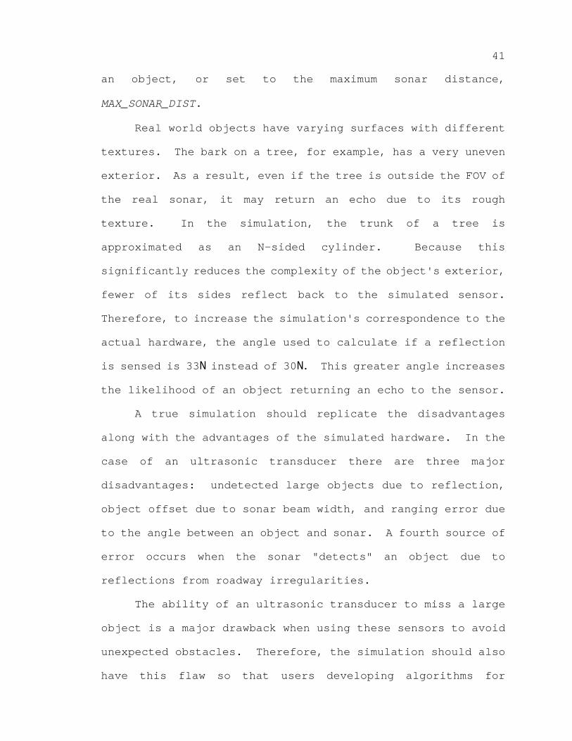
The ability of an ultrasonic transducer to miss a large

object is a major drawback when using these sensors to avoid

unexpected obstacles. Therefore, the simulation should also

have this flaw so that users developing algorithms for

42

Figure 5-1: Simulation ofundetected large object due toreflection.

obstacle avoidance can accurately fine tune these algorithms

in the simulated world before applying them to the "real"

world. Figure 5-1 show this flaw in an extreme case. From

the figure, it can be seen that all sixteen sensors completely

miss the large object. This was a special case, since two or

three sensors picked up the object when the vehicle was

rotated slightly to the left or right. Figure 5-2 shows an

example of object offset. The object is offset, but normal to

the transmitted beam, causing an error in the x component.

The sensor is detecting the plane whose normal is parallel

43

Figure 5-2: Simulation of objectoffset due to beam width.

with the sonar's vector, but from the figure it can be seen

the object is offset from the beam's center.

Range error due to the angle between an object and the

sonar is shown in figure 5-3. This error arises because the

range computed is the closest distance to the object within

the FOV of the sonar, and not the range from the center line

of the beam. This is shown graphically because the sonar cone

representing the range is extends only to the distance where

the cone first meets the plane, and not to the distance from

the center line.

The simulated version of the last disadvantage, "phantom"

echoes from roadway irregularities, occurs as a consequence of

round off errors. Since all primitives are drawn using flat

planes, if the user wished to incorporate "phantom" echoes,

44

Figure 5-3: Simulation of range error dueto angle between object and sonar.

he/she would have to create multi-faceted surfaces.

Fortunately, round off errors make this unnecessary. Since

mapw uses the low precision x and y screen coordinates

(variable type short) to determine the line in space, errors

develop in this backward transformation. These errors, in

turn, cause miscalculations when determining the angle between

the "detected" object and the sonar normal. Every so often

these angles fall within tolerance and cause a return echo to

be detected by the sensor. These phantom echoes can be

increased, slightly, by including the floor as one of the

unexpected obstacles. This ensures there is always at least

one object to cause a return echo. Figure 5-4 shows this

phenomenon, which only happens occasionally. The number of

45

Figure 5-4: Simulation of phantom echo.

phantom echoes can be increased by scattering small blocks

along the floor to reflect the sound back to the sensor.

Laser Range Scanner

The Perceptron LASAR camera converts a real world scene

into two and three dimensional information. Therefore, the

most important parameter is the accurate determination of

range. The range is correctly determined from the floating

point transformed z data returned by feedbuf. The only

difference between the simulated range data and the data

returned by the Perceptron LASAR is the amount of bits used to

store the data. The Perceptron stores the numbers with 12 bit

accuracy, while in the simulation the range is stored in a 32

bit floating point number. This 32 bit floating point number

is reduced to an 8 bit color scale, since there is only a 256

color gray scale. Figure 5-5 shows a world view of the planes

46

Figure 5-5: World view of laser range scanner'stest planes.

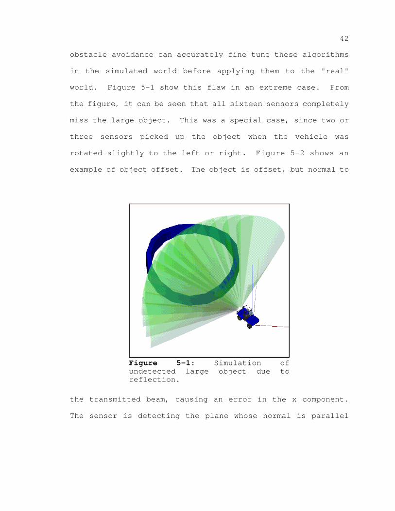
used to test the laser range scanner. The four planes are 10

meters high, and each successive one is 5 meters higher and

five meters farther away then the last one. This is

illustrated in figure 5-6 which is taken from the point of

view of the driver. The laser range scanner is located

directly overhead, and in front of the vehicle are the four

planes. The image created by the laser range scanner should

be have four distinct colors representing the four different

distances of the test planes.

47

Figure 5-6: Scene from the point of view of thedriver.

Figure 5-7 shows the actual graphical representation of

the range data from the laser range scanner. In the test, the

ground was included as an unexpected obstacle. This causes

the floor in the scanned image to appear increasingly dark as

it extends away from the scanner. The four planes can be seen

as four distinct color areas, each progressively darker. The

last plane is close to the MAX_LRS_DIST and is thus dark and

hard to see.

The one disadvantage of the laser range scanner is the

effect that a flat featureless wall has on range data. This

wall produces range "rings" due to geometry of the scanning

48

Figure 5-7: Image created by the simulatedlaser range scanner.

laser. Since the test objects were large flat planes, this

effect should also be visible. Figure 5-7 shows these rings

in the simulated laser range scanner. These concentric

circles can be seen on each of the four planes. The bottom

one-third of the image consists of the scanned floor, which

gradually decreases in tone the further away the floor is from

the scanner. The bottom of the first of the four planes

begins with the noticeable line running across the lower half

of the image. The tops of the four planes can be seen as the

color jumps to a darker tone. Since the last plane is close

to the maximum distance, 40 meters, it is a dark gray against

a black background, and therefore hard to see. By careful

49

comparison of the centers of each plane with their

corresponding edges, the concentric circles can be seen.

Since the resolution in the simulation is lower than the

actual hardware, the effect is not as pronounced

5.2 Conclusions

A computer simulation of hardware should accurately

emulate the hardware's function in real time. When a

simulation does this, the transition from the simulation to

the real world is slight and uncomplicated. The results

obtained from the simulation can accurately be transformed to

the hardware. "What-if" scenarios can be performed on the

simulation. Simulations also have many other advantages. In

a simulated world view, the point of view can be changed on-

the-fly to view the scene from any location and at any

altitude. In this simulation, a scene can be observed from

the point of view of the driver, or from any point in the

simulated environment.

Sonar

The current simulation of an ultrasonic transducer, or

sonar, accurately determines the range to the nearest

obstacle. It also mimics the problems associated with using

ultrasonic transducers to detect objects. Currently, real

time calculations of the range data for the sonar array are

slowed by two factors: the way in which range data are

50

calculated for each sonar, and the number of unexpected

obstacles.

Range data is calculated for each sonar by first drawing

the scene from the point of view of the sonar in a perspective

projection. If any obstacles are detected within the viewing

volume, the scene is then drawn five times with an

orthographic projection to determine the range and angle.

Consequently, with only one ultrasonic transducer, as the

vehicle approaches an unexpected object, the scene is redrawn

six times instead of one. For instance, if each transducer in

an array of three detects an object within its viewing volume,

the simulated world is redrawn 18 times. These repeated

redrawing noticeably decrease the number of frames which can

be drawn per second.

Since every unexpected obstacle must be drawn each time

range data is needed, the quantity of unexpected obstacles has

a direct effect on the speed of the simulation. Even in a

simple scene the number of objects can be large. For example,

a cylinder can be represented by a 12-sided polygon with two

ends. Thus 14 planes are drawn on the screen. The test world

in the simulation contains 16 objects resulting in a total of

128 planes. While the delay is not excessive, a noticeable

decrease in the speed of the vehicle can be observed.

Currently the sonar simulation is in use by Arturo

Rankin, who is working on path planning and path execution for

an autonomous nonholonomic robot vehicle. The simulation has

51

helped him fine tune the algorithms used to avoid unexpected

obstacles. He and David Armstrong, who worked on the

ultrasonic transducers, helped in correlating the simulation's

data with actual data.

Laser Range Scanner

The current LRS simulation can scan a scene and

accurately determine the range associated with each pixel in

the image window. The simulation also displays concentric

circles when scanning a flat featureless wall. Unfortunately,

real time scanning is currently not possible due to the amount

of time the scene needs to be redrawn. In the simulation, the

unexpected obstacles need to be redrawn 65,536 times, since

the window is 256 by 256. This results in a scan time of 5

minutes. The Perceptron LASAR can scan a 1024 by 1024 scene

in 5.6 seconds. As the number of unexpected obstacles

increases, the image scan time also increases.

52

5.3 Future Goals

There are certain areas in the simulation which can

improve the real time response and overall simulation of the

hardware:

1. At present, the real time response of the sonarsimulation is hindered as the number of sonar sensors isincreased. This occurs largely because once an object islocated within the FOV of the sensor, five orthographicprojections are drawn for each sensor detecting anunexpected obstacle. Currently work is being done toreduce the number of orthographic projections drawn foreach sensor to one. Thus the unexpected obstacles wouldonly be redraw twice, once for the perspective projectionand once for the orthographic projection.

2. Only a single echo from an object is analyzed becauseof the computing time required. The simulation would haveto calculate the angle of the object and the reflectedecho, then redraw the scene from the point of view of theecho from the next object, and so on, to determine if anyechoes will reach the sensor and give a false range.Initially this was not completed since each sonar timesout after the period required to reach the maximum rangeis reached.

3. The Perceptron LASAR camera also displays a 2Dintensity image of the scanned scene. Once the anglebetween the sensor and the surface normal is known, thisangle can be used to determine the magnitude for theintensity data.

4. The number of unexpected objects that must be redrawncan be decreased using the location of the vehicle. Bystoring the location and size of the bounding boxes ofthe unexpected objects, the location of the field of viewof the sensor can be used to determine which objectsmight be detected by the sensor. This technique wouldnot be practical for sonar, but would be useful for theLRS. Since sonar sensors could be located anywhere, theintersections would have to be computed for each sensor.LRS, on the other hand, scans a fixed area a large numberof times.

53

REFERENCES

And90 Andersen, Claus S., Madsen, Claus B., Sorensen, JanJ., Kirkeby, Neils O.S., Jones, Judson P., andChristensen, Henrik I., Navigation Using RangeImages on a Mobile Robot, U.S. Department ofEnergy, contract # DE-AC05-84OR21400 Oak Ridge, TN,(1990).

Ara83 Arai, Tatsuo, and Nakano, Eiji, "Development ofMeasuring Equipment for Location and DirectionUsing Ultrasonic Waves," Journal of DynamicSystems, Measurment, and Control, 105(1983):152-156.

Bec92 Beckerman, M., and Sweeney, F.J., Restoration andFusion of Laser Range Camera Images, EngineeringPhysics and Mathematics Division, U.S. Departmentof Energy Oak Ridge, TN, (1992).

Bro89 Brown, Mark, "US Air Force Relies on ComputerGraphics to Evaluate Combat Aircraft Performance,"IEEE Computer Graphics and Applicatons, 9(1988):10-11.

Cul89 Culviner, Tom, "Graphics Windows for ConcurrentSimulation," IEEE Computer Graphics andApplications, 9(1989):8-9.

Gri91 Grinstein, Geroges, "Notes on MultisensoryVisualization Systems," IEEE Computer Graphics andApplications, 11(1991):18-19.

Hui89 Huissoon, J.P. and Moziar, D.M., "Curved UltrasonicArray Transducer for AGV Applications,"Ultrasonics, 27(1989):221-225.

Kat81 Kattan, Shalom, A Microcomputer Controlled AcousticProximity Detector, Master's Thesis, University ofFlorida, Gainesville, FL, (1981).

Kwe91 Kweon, In So, Hoffman, Regis, and Kortkov, Eric,Experimental Characterization of the PerceptronLaser Rangefinder, technical report CMU-RI-TR-91-1Carnegie Mellon University, Pittsburg (1991).

Mor89 Moring, I., Heikkinen, T., Myllyla, R.,"Acquisition of Three-Dimensional Image Data by aScanning Laser Range Finder," Optical Engineering,8, 28(1989):897-902.

54

Mun89 Munro, W.S.H., Pomeroy, S., Rafiq, M., Williams,H.R., Wybrow, M.D., and Wykes, C., "UltrasonicVehicle Guidance Transducer," Ultrasonics,28(1990):350-354.

Nar90 Nagai, Keiosuke and Greenleaf, James F.,"Ultrasonic Imaging Using the Doppler Effect Causedby a Moving Transducer," Optical Engineering, 10,29(1990):1249-1254.

Nis86 Nishide, Kenichi, Hanawa, Moritomo, and Kondo,Toshio, Automatic Position Findings of Vehicle byMeans of Laser, Research and DevelopmentDepartment, Tokyo Aircraft Instrument Co., Ltd,Tokyo, Japan, (1986)

Par91 Parkin, Robert E., "An Interactive RoboticSimulation Package," Simulation, 56(1991):337-345.

Per92 Perceptron, High Resolution 2-D and 3-D Images froma single Camera, Perceptron, Farmington Hills, MI,(1992).

Pol80 Polaroid Corporation, Environmental UltrasonicTransducer, Polariod Corporation, Cambridge, MA(1980).

Poo89 Poole, Harry H., Fundamentals of RoboticsEngineering, Van Nostrand Reinhold, New York,(1989).

Rac89 Raczkowsky, J., and Mittenbuebuehler, K.H.,"Simulation of Cameras in Robot Applications," IEEEComputer Graphics and Applications, 9(1989):16-25.

Reu91 Reuter, Guido P. An Expandable Mobile Robot Systemwith Sonar-Based Map-Building and NavigationCapabilities, Master Thesis, University of Florida,Gainesville, (1991).

Rio91 Rioux, Marc, Beraldin, J. Angelo, O'Sullivan, M.,and Cournoyer, L., "Eye-safe Laser Scanner forRange Imaging," Applied Optics, 16, 30(1991):2219-2223.

San92 Sangalli, Arturo, "Computer gives Robot's Eye Viewof Optical Surgery," Technology 134(1992):22.

Sil91 Silicon Graphics Inc., Graphics Library ProgrammingGuide, Silicon Graphics, Mountain View, CA, (1991).

55

Swe91 Sweeny, F.J., Random and Systematic Errors in LaserRange Camera Data, Center for Engineering SystemsAdvanced Research, Oak Ridge National LaboratoryOak Ridge, TN, (1991).

Tho88 Thompson, Gerald A., "Interactive ComputerGraphics," Aerospace America, 26(1988):29

Wal87 Walter, Scott A., The Sonar Ring: ObstacleDetection for a Mobile Robot, Computer ScienceDepartment, General Motors Research Laboratories,Warren, MI (1987).

Whi89 Whitehouse, J.C., "New Principle of RangefindingUsing Blurred Images," Journal of Physics. D,Applied Physics, 22(1989):11-22.

Whi90 Whitehose, J.C., "Range Information Using BlurredImages," Journal of Physics. D, Applied Physics,23(1990):1342-9.

Wil90 Wilhelms, Jane and Skinner, Robert, "A 'Notion' forInteractive Behavioral Animation Contorl," IEEEComputer Graphics and Applications, 10(1990):14-22.

56

BIOGRAPHICAL SKETCH

David Keith Novick was born on January 4, 1968, in

Hollywood, Florida. He received the Bachelor of Science in

Mechanical Engineering with honors in May 1991 at the

University of Florida (UF). In August 1991, he entered the

master's program in mechanical engineering at UF. Upon

completion of the Master of Engineering, he intends to pursue

a doctoral degree in mechanical engineering at UF.

I certify that I have read this study and that in myopinion it conforms to acceptable standards of scholarlypresentation and is fully adequate, in scope and quality, asa thesis for the degree of Master of Engineering.

Carl D. Crane III, ChairAssociate Professor of Mechanical Engineering

I certify that I have read this study and that in myopinion it conforms to acceptable standards of scholarlypresentation and is fully adequate, in scope and quality, asa thesis for the degree of Master of Engineering.

Joseph DuffyGraduate Research Professor of Mechanical Engineering

I certify that I have read this study and that in myopinion it conforms to acceptable standards of scholarlypresentation and is fully adequate, in scope and quality, asa thesis for the degree of Master of Engineering.

Kevin Scott SmithAssociate Professor of Mechanical Engineering

This thesis was submitted to the Graduate Faculty of theCollege of Engineering and to the Graduate School and wasaccepted as partial fulfillment of the requirements for thedegree of Master of Engineering.

August 1993 Winfred M. PhillipsDean, College of Engineering

Dean, Graduate School

58