INTERACTION DOMAIN OF SHALLOW FOUNDATIONS ON THE TOP OF A SLOPE

Academic Year 2013-2014

POLITECNICO DI MILANO Department of Civil, Environmental and Land Management Engineering

Master of Science in Civil Engineering

Supervisor: Prof. Andrea Galli

Master Dissertation of:

Mehdi Nouri / 770776

To my beloved family.

i

Acknowledgments Foremost, I would like to express my sincere gratitude and deepest appreciation to my advisor Professor Andrea Galli for the continuous support of my Master dissertation, for his patience, motivation, enthusiasm, and immense knowledge. His guidance helped me in all the time of research and writing of this thesis. I could not have imagined having a better advisor and mentor for my Master study. Many friends have helped me stay sane through these difficult years. Their support and care helped me overcome setbacks and stay focused on my graduate study. I greatly value their friendship and I deeply appreciate their belief in me. Last but by no means least, a special heart-felt gratitude to my family. Words cannot express how grateful I am to my father, my mother and my brothers for all of the sacrifices that they’ve made on my behalf. Their unequivocal love and support throughout, as always, for which my mere expression of thanks does not suffice.

ii

Abstract The bearing capacity of the foundation is a primary concern in the field of

foundation engineering. Structures may be built on or near slopes due to either land limitation issues, such as in retaining walls and bridges abutments, or architectural purposes. The ultimate bearing capacity of the foundation for these buildings is significantly affected by the presence of the slope. Design of foundation under these conditions is complex and the information available in the literature is limited.

A numerical model has been developed to simulate the case of strip foundation near slope, using the explicit finite difference software “FLAC”, considering the constitutive law of soil as elastic-perfectly plastic. The parameters which govern this behavior were examined individually in order to determine their effects on the ultimate bearing capacity and the interaction locus of vertical and horizontal loads of a strip footing. Totally 328 models are simulated in the program for different granular soils. Initially, some calibrations have been done in order to find the optimum case of simulating model. Soil domain size, number of meshes in soil volume, and velocity of loading were calibrated. Subsequently, various parameters in simulation related to geometry and soil properties are changed, such as load inclination angle with vertical, different slope angles, different distance of foundation to the slope edge, different angles of frictions, and different dilation angles. Afterwards, the results produced by the program are compared and validated with available theoretical solutions in order to verify the quality of the results obtained from the program.

An analytical solution considering the effects of slope is proposed for the problem stated to predict the interaction domain of a strip footing resting near a slope. Along with, a design chart is developed to predict the ultimate bearing capacity of a shallow foundation taking into account dilation angle which was not considered in the previous works. Design theory, design procedure, and design charts are provided for practical use. Key Words: Interaction Locus, Shallow Foundation, FLAC, Slope Stability, Foundation on top of a Slope, Soil-structure Interaction, Numerical Analysis, Bearing Capacity

iii

Sommario Il calcolo della capacità portante delle fondazioni superficiali è un tema

centrale in Ingegneria Geotecnica. A causa di vari fattori limitanti, o di scelte urbanistiche o architettoniche, le strutture possono essere costruite in prossimità di pendii, come nel caso di muri di sostegno o pile da ponte. La capacità portante ultima della fondazione di queste strutture è significativamente influenzata dalla presenza del pendio. La progettazione delle opere di fondazione in queste condizioni è complessa e le informazioni disponibili in letteratura è limitata.

Un modello numerico è stato sviluppato per simulare il caso della fondazione nastriforme vicino ad un pendio, utilizzando il software esplicito alle differenze finite "FLAC", considerando la legge costitutiva del terreno elastico perfettamente plastico. I parametri che governano il problema sono stati esaminati singolarmente per determinare i loro effetti sulla capacità portante ultima e sul dominio di interazione tra carichi verticali e orizzontali agenti sulla fondazione. In totale 328 modelli sono stati simulate nel programma per diversi terreni granulari. Inizialmente, alcune calibrazioni sono state fatte al fine di ottimizzare la simulazione in termini di dimensione e discretizzazione del dominio, di velocità di carico, ecc.

Successivamente, i vari parametri di simulazione relativi alla geometria e del terreno sono stati fatti variare, come angolo di inclinazione dei carichi sulla verticale, pendenza del pendio, distanza della fondazione dal ciglio, diversi angoli di attrito del materiale e di dilatanza. Successivamente, i risultati prodotti dal programma sono stati confrontati e con soluzioni teoriche disponibili in letteratura. Parole chiave: Dominio di Interazione, Fondazioni Superficiali, Analisi Numeriche, Interazione terreno-fondazione in Prossimità di un Pendio

iv

Table of Contents Acknowledgments ........................................................................................................... i

Abstract .......................................................................................................................... ii

Sommario ..................................................................................................................... iii

List of Figures ....................................................................................................... vii

List of Tables ........................................................................................................ xiii

List of Notations ................................................................................................... xv

1. Introduction ................................................................................................. 1

1.1 Outline of the Study ......................................................................................... 1

1.2 Background Information .................................................................................. 1

1.2.1 Foundations ............................................................................................... 2

1.2.2 Shallow Foundation .................................................................................. 2

1.2.3 Bearing Capacity ....................................................................................... 3

1.2.4 Allowable Bearing Capacity ...................................................................... 4

1.2.5 Ultimate Bearing Capacity ....................................................................... 5

1.2.5.1 General Failure ........................................................................................... 6

1.2.5.2 Local Failure ............................................................................................... 6

1.2.5.3 Punching Failure ........................................................................................ 7

1.2.6 Inclined Loading ........................................................................................ 8

1.3 Research Objectives .......................................................................................... 9

1.4 The Procedure ................................................................................................... 9

1.5 Chapters Overview ......................................................................................... 10

1.5.1 Chapter 1 – Introduction ........................................................................ 10

1.5.2 Chapter 2 - Literature Review ............................................................... 10

1.5.3 Chapter 3 – Introduction to FLAC and Numerical Modeling .............. 10

1.5.4 Chapter 4 – The Results and Analysis ................................................... 10

1.5.5 Chapter 5 – Conclusion ........................................................................... 10

1.6 Summary ......................................................................................................... 11

2. Literature Review ..................................................................................... 12

2.1 General ............................................................................................................ 12

2.2 Previous Theories ........................................................................................... 12

2.2.1 Bearing Capacity for Purely Vertical Loading ...................................... 12

2.2.1.1 Terzaghi’s Bearing Capacity Theorem .................................................... 12

2.2.1.2 Meyerhof’s Bearing Capacity Theorem ................................................... 15

2.2.1.3 Hansen’s and Vesic’s Bearing Capacity Theorems ................................ 17

v

2.2.1.4 Other Theories for Finding Bearing Capacity ........................................ 18

2.2.2 Bearing Capacity for Inclined Loading .................................................. 20

2.2.2.1 Meyerhof’s Theory .................................................................................... 20

2.2.2.2 Hansen’s Theory ....................................................................................... 21

2.2.2.3 Vesic’s Solution ......................................................................................... 21

2.2.3 Bearing Capacity for Foundation on Top of a Slope ............................. 21

2.2.3.1 Meyerhof’s Solution .................................................................................. 21

2.2.3.2 Solution of Vesic and Hansen .................................................................. 22

2.2.3.3 Limit Equilibrium and Limit Analysis Solution .................................... 22

2.2.3.4 Stress Characteristics Solution................................................................ 24

2.2.3.5 Other Solutions ......................................................................................... 26

2.2.4 Horizontal Bearing Capacity .................................................................. 28

2.3 Interaction Locus of Bearing Capacities ....................................................... 29

2.3.1 Interaction Locus of Horizontal Ground ............................................... 29

2.3.2 Interaction Locus of Sloped Ground ...................................................... 33

2.4 Summary ......................................................................................................... 35

3. Introduction to FLAC and Numerical Modeling ................................. 36

3.1 Introduction .................................................................................................... 36

3.2 Fast Lagrangian Analysis of Continua .......................................................... 36

3.2.1 Key Features of FLAC ............................................................................ 37

3.3 Problem Definition ......................................................................................... 37

3.4 Producing Numerical Models within FLAC ................................................. 37

3.4.1 Making Geometry .................................................................................... 38

3.4.2 Applying Loads ........................................................................................ 41

3.4.3 Modeling the Slopes ................................................................................ 43

3.5 Running the Model ......................................................................................... 47

3.6 Summary ......................................................................................................... 47

4. Results and Analysis ................................................................................. 48

4.1 Introduction .................................................................................................... 48

4.2 Theoretical Results ......................................................................................... 48

4.2.1 Foundation on Horizontal Ground ........................................................ 48

4.2.2 Foundation on the Top of a Slope .......................................................... 51

4.3 Calibrations ..................................................................................................... 55

4.2.1 Meshing Alignment ................................................................................. 56

4.2.2 Velocity Calibration ................................................................................ 57

4.2.3 Width and Depth Calibration ................................................................. 57

vi

4.3 Loose Sand ...................................................................................................... 59

4.3.1 Horizontal Ground .................................................................................. 59

4.3.2 “b=0 m” ................................................................................................... 60

4.3.3 “b=1 m” ................................................................................................... 61

4.3.4 “b=2 m” ................................................................................................... 62

4.3.5 “b=4 m” ................................................................................................... 63

4.3.6 “b=8 m” ................................................................................................... 64

4.3.7 Comparison of Performed Tests............................................................. 65

4.3.7.1 Different Values of b ................................................................................. 65

4.3.7.2 Different Values of Slope Angle (β) ......................................................... 67

4.4 Dense Sand ...................................................................................................... 69

4.4.1 Horizontal Ground .................................................................................. 69

4.4.2 “b=0 m” ................................................................................................... 70

4.4.3 “b=1 m” ................................................................................................... 71

4.4.4 “b=2 m” ................................................................................................... 72

4.4.5 “b=4 m” ................................................................................................... 73

4.4.6 “b=8 m” ................................................................................................... 74

4.4.7 Comparison of Performed Tests............................................................. 75

4.4.7.1 Different Values of b ................................................................................. 75

4.4.7.2 Different Values of Slope Angle (β) ......................................................... 77

4.5 Validations with Theoretical Solutions ......................................................... 79

4.6 Developing an Analytical Solution ................................................................ 92

4.7 Proposing a Design Chart ............................................................................ 103

5. Conclusion ................................................................................................ 105

References ....................................................................................................... 107

vii

List of Figures Figure 1-1 - A scheme of shallow foundation .............................................................. 3 Figure 1-2 - Different types of shallow foundations, (a) Spread Footing, (b) Strip Footing (c) Grade Beams (d) Mat Footing .................................................... 3 Figure 1-3 - Idealized axial load-displacement-capacity response of shallow foundations. ................................................................................................................... 4 Figure 1-4 - Definition sketch of dimensions for a footing ......................................... 4 Figure 1-5 - Methods for determining the bearing capacity of shallow foundations .................................................................................................................... 5 Figure 1-6 - Boundaries of zone of plastic equilibrium after failure of Soil Beneath Continuous Footing. ....................................................................................... 6 Figure 1-7 – Modes of bearing capacity failure (After Vesic, 1975) ........................... 7 Figure 1-8 - Nature of failure in soil with relative density of sand Dr and Df/R. ................................................................................................................................ 8 Figure 1-9 - A general scheme of shallow foundations with (a) Vertical loading (b) Inclined loading (both vertical and horizontal loading) .......................... 8 Figure 1-10 - Problem notation and potential failure mechanism. ........................... 9 Figure 2-1 - Modified failure surface in soil supporting a shallow foundation at ultimate load. ....................................................................................... 15 Figure 2-2 - Slip line fields for a rough continuous foundation. .............................. 15 Figure 2-3 - Comparison of Nγ Values for Shallow Foundation according to Terzaghi, Meyerhof, Vesic and Hansen ................................................................ 18 Figure 2-4 - Comparison of Nγ Values for Shallow Foundation according to Chen, Kumar, Michalowski, Hjiaj et al. and Martin. .......................................... 20 Figure 2-5 - Plastic zones in soil near a foundation with an inclined load. ............ 20 Figure 2-6 - Meyerhof’s bearing capacity factor, (a) Ncq for purely cohesive soil and (b) Nγq for granular soil [13]. ......................................................... 22 Figure 2-7 - Forces of Elastic Wedge ADE ................................................................. 23 Figure 2-8 - Rupture Surface Assumed in Limit Equilibrium and Limit Analysis Approaches. .................................................................................................. 23 Figure 2-9 - Typical results after Andrew's procedures. ........................................... 25 Figure 2-10 - Graham's asymmetric failure mechanism geometry [13] .................. 25 Figure 2-11 - A scheme of failure zones for embedment and setback: (a) Df/B > 0; (b) b/B > 0 [13] ............................................................................................ 25 Figure 2-12 - Graham, Andrews and Shields theoretical values of Nγq (Df/B=0) [22] ................................................................................................................ 26 Figure 2-13 - Reduction coefficient iβ for bearing capacity factor Nγq according to Garnier et al. researches. Note that the terms tanφ and tanβ represent the function of tan(φ) and tan(β) respectively. ........................................ 27 Figure 2-14- Comparison of Different Horizontal Bearing Capacities presented by Butterfield. ............................................................................................ 29 Figure 2-15 - Interaction Locus of (a) Horizontal Bearing Capacity vs Vertical Bearing Capacity, (b) Horizontal Bearing Capacity and Momentum vs Vertical Bearing Capacity , proposed by Ticof ................................. 30 Figure 2-16 - Interaction Locus of Horizontal Loading vs. Moment ....................... 31 Figure 2-17 - Interaction Locus for Simplified Vertical Load vs. Horizontal Load, or Moment. ........................................................................................................ 32

viii

Figure 2-18 - Best fit Ellipse for Normalized "n-m" Plot .......................................... 32 Figure 2-19 - Failure Locus of V-H plane for Pipeline-Soil Interaction on Horizontal Ground ...................................................................................................... 33 Figure 2-20 - Failure Locus of V-H Plane for Pipeline-Soil Interaction by Calvetti et al. ................................................................................................................ 34 Figure 2-21 - Failure Locus for V-H plane for Pipeline-Soil Interaction by di Prisco & Galli .......................................................................................................... 34 Figure 2-22 - Failure Locus for V-H Plane for Pipeline-Soil Interaction by Merifield et al. .............................................................................................................. 34 Figure 2-23 - Failure Locus for V-H Plane for Pipeline-Soil Interaction by di Prisco et al. .............................................................................................................. 35 Figure 3-1 - The first five steps before applying the loading to the model ............. 38 Figure 3-2 - Mohr-Coulomb Failure Criterion. ......................................................... 39 Figure 3-3 - The element is dilating during shear. This plastic behavior. (Referring to Salgado, the Engineering of Foundations) ......................................... 39 Figure 3-4 - The initial stress along Y direction. ...................................................... 41 Figure 3-5 - The scripts used for applying forces, part 1. ......................................... 42 Figure 3-6 - The scripts used for applying forces, part 2. ......................................... 43 Figure 3-7 - A model produced by using the indicated codes. .................................. 43 Figure 3-8 - The supplementary part of the scripts for modeling the slope. .......... 44 Figure 3-9 - A sloped model produced by using the supplementary codes. ............. 44 Figure 3-10 - A scheme of different geometries simulated in this thesis. ............... 45 Figure 3-11 - A scheme of different loading cases simulated in this thesis. ........... 47 Figure 4-1 - The scheme of a foundation near a slope with needed notations. ..................................................................................................................... 48 Figure 4-2 - Different bearing capacities for various soil volume sizes, Loose Sand. .................................................................................................................. 56 Figure 4-3 - Meshing Alignment for loose sand ........................................................ 56 Figure 4-4 – Velocity Alignment, Loose sand. ........................................................... 57 Figure 4-5 - Width Alignment, loose sand. ................................................................ 58 Figure 4-6 - Depth Alignment, loose sand. ................................................................ 58 Figure 4-7 - Direction of the positive side of graphs. ................................................ 59 Figure 4-8 - Interaction Locus for Horizontal Ground, Loose Sand ....................... 59 Figure 4-9 - Interaction Locus of 10° slope and b=0m, Loose Sand. ....................... 60 Figure 4-10 - Interaction Locus of 20° slope and b=0m, Loose Sand. ..................... 60 Figure 4-11 - Interaction Locus of 30° slope and b=0m, Loose Sand. ..................... 60 Figure 4-12 - Interaction Locus of 10° slope and b=1m, Loose Sand. ..................... 61 Figure 4-13 - Interaction Locus of 20° slope and b=1m, Loose Sand. ..................... 61 Figure 4-14 - Interaction Locus of 30° slope and b=1m, Loose Sand. ..................... 61 Figure 4-15 - Interaction Locus of 10° slope and b=2m, Loose Sand. ..................... 62 Figure 4-16 - Interaction Locus of 20° slope and b=2m, Loose Sand. ..................... 62 Figure 4-17 - Interaction Locus of 30° slope and b=2m, Loose Sand. ..................... 62 Figure 4-18 - Interaction Locus of 10° slope and b=4m, Loose Sand. ..................... 63 Figure 4-19 - Interaction Locus of 20° slope and b=4m, Loose Sand. ..................... 63 Figure 4-20 - Interaction Locus of 30° slope and b=4m, Loose Sand. ..................... 63 Figure 4-21 - Interaction Locus of 10° slope and b=8m, Loose Sand. ..................... 64 Figure 4-22 - Interaction Locus of 20° slope and b=8m, Loose Sand. ..................... 64 Figure 4-23- Interaction Locus of 30° slope and b=8m, Loose Sand. ...................... 64

ix

Figure 4-24 - Comparison of Interaction Locus for b=0m with Different Angles, "Loose" Sand ................................................................................................... 65 Figure 4-25 - Comparison of Interaction Locus for “b=1m” with Different Angles, "Loose" Sand ................................................................................................... 65 Figure 4-26 - Comparison of Interaction Locus for “b=2m” with Different Angles, "Loose" Sand ................................................................................................... 66 Figure 4-27 - Comparison of Interaction Locus for “b=4m” with Different Angles, "Loose" Sand ................................................................................................... 66 Figure 4-28 - Comparison of Interaction Locus for “b=8m” with Different Angles, "Loose" Sand ................................................................................................... 66 Figure 4-29- Comparison of Interaction Locus for “β=10°” with Different b, "Loose" Sand............................................................................................................. 67 Figure 4-30- Comparison of Interaction Locus for “β=20°” with Different b, "Loose" Sand............................................................................................................. 67 Figure 4-31- Comparison of Interaction Locus for “β=30°” with Different b, "Loose" Sand............................................................................................................. 67 Figure 4-32 - Comparison of different b and β vs. Vm ............................................. 68 Figure 4-33 - Interaction Locus for Horizontal Ground, Dense Sand. .................... 69 Figure 4-34 - Interaction Locus of 10° slope and b=0m, Dense Sand. .................... 70 Figure 4-35 - Interaction Locus of 20° slope and b=0m, Dense Sand. .................... 70 Figure 4-36 - Interaction Locus of 30° slope and b=0m, Dense Sand. .................... 70 Figure 4-37 - Interaction Locus of 10° slope and b=1m, Dense Sand. .................... 71 Figure 4-38 - Interaction Locus of 20° slope and b=1m, Dense Sand. .................... 71 Figure 4-39 - Interaction Locus of 30° slope and b=1m, Dense Sand. .................... 71 Figure 4-40 - Interaction Locus of 10° slope and b=2m, Dense Sand. .................... 72 Figure 4-41 - Interaction Locus of 20° slope and b=2m, Dense Sand. .................... 72 Figure 4-42 - Interaction Locus of 30° slope and b=2m, Dense Sand. .................... 72 Figure 4-43 - Interaction Locus of 10° slope and b=4m, Dense Sand. .................... 73 Figure 4-44 - Interaction Locus of 20° slope and b=4m, Dense Sand. .................... 73 Figure 4-45 - Interaction Locus of 30° slope and b=4m, Dense Sand. .................... 73 Figure 4-46 - Interaction Locus of 10° slope and b=8m, Dense Sand. .................... 74 Figure 4-47 - Interaction Locus of 20° slope and b=8m, Dense Sand. .................... 74 Figure 4-48 - Interaction Locus of 30° slope and b=8m, Dense Sand. .................... 74 Figure 4-49 - Comparison of Interaction Locus for “b=0m” with Different Angles, "Dense" Sand ................................................................................................... 75 Figure 4-50 - Comparison of Interaction Locus for “b=1m” with Different Angles, "Dense" Sand ................................................................................................... 75 Figure 4-51 - Comparison of Interaction Locus for “b=2m” with Different Angles, "Dense" Sand ................................................................................................... 76 Figure 4-52 - Comparison of Interaction Locus for “b=4m” with Different Angles, "Dense" Sand ................................................................................................... 76 Figure 4-53 - Comparison of Interaction Locus for “b=8m” with Different Angles, "Dense" Sand ................................................................................................... 76 Figure 4-54 - Comparison of Interaction Locus for “β=10°” with Different b, "Dense" Sand ............................................................................................................ 77 Figure 4-55 - Comparison of Interaction Locus for “β=20°” with Different b, "Dense" Sand ............................................................................................................ 77

x

Figure 4-56 - Comparison of Interaction Locus for “β=30°” with Different b, "Dense" Sand ............................................................................................................ 77 Figure 4-57 - Comparison of different b and β vs. Vm ............................................. 78 Figure 4-58 - Comparison of Interaction Locus for “Loose” Sand and “Dense” Sand ............................................................................................................... 78 Figure 4-59 - Different Bearing Capacities on Horizontal Ground Proposed by Different Authors, “Loose” Sand ......................................................... 79 Figure 4-60 - Different Bearing Capacities on Horizontal Ground Proposed by Different Authors, “Dense” Sand ........................................................ 79 Figure 4-61 - Comparison of Numerical Results with Theoretical Values, "Loose" Sand. ................................................................................................................ 80 Figure 4-62 - Comparison of Numerical Results with Theoretical Values, "Dense" Sand. ............................................................................................................... 80 Figure 4-63 - Comparison of Numerical Results with Theoretical Values, b=0m and β=10°, "Loose" Sand. ................................................................................ 81 Figure 4-64 - Comparison of Numerical Results with Theoretical Values, b=0m and β=20°, "Loose" Sand. ................................................................................ 81 Figure 4-65 - Comparison of Numerical Results with Theoretical Values, b=0m and β=30°, "Loose" Sand. ................................................................................ 81 Figure 4-66 - Comparison of Numerical Results with Theoretical Values, b=1m and β=10°, "Loose" Sand. ................................................................................ 82 Figure 4-67 - Comparison of Numerical Results with Theoretical Values, b=1m and β=20°, "Loose" Sand. ................................................................................ 82 Figure 4-68 - Comparison of Numerical Results with Theoretical Values, b=1m and β=30°, "Loose" Sand. ................................................................................ 82 Figure 4-69 - Comparison of Numerical Results with Theoretical Values, b=2m and β=10°, "Loose" Sand. ................................................................................ 83 Figure 4-70 - Comparison of Numerical Results with Theoretical Values, b=2m and β=20°, "Loose" Sand. ................................................................................ 83 Figure 4-71 - Comparison of Numerical Results with Theoretical Values, b=2m and β=30°, "Loose" Sand. ................................................................................ 83 Figure 4-72 - Comparison of Numerical Results with Theoretical Values, b=4m and β=10°, "Loose" Sand. ................................................................................ 84 Figure 4-73 - Comparison of Numerical Results with Theoretical Values, b=4m and β=20°, "Loose" Sand. ................................................................................ 84 Figure 4-74 - Comparison of Numerical Results with Theoretical Values, b=4m and β=30°, "Loose" Sand. ................................................................................ 84 Figure 4-75 - Comparison of Numerical Results with Theoretical Values, b=8m and β=10°, "Loose" Sand. ................................................................................ 85 Figure 4-76 - Comparison of Numerical Results with Theoretical Values, b=8m and β=20°, "Loose" Sand. ................................................................................ 85 Figure 4-77 - Comparison of Numerical Results with Theoretical Values, b=8m and β=30°, "Loose" Sand. ................................................................................ 85 Figure 4-78 - Comparison of Numerical Results with Theoretical Values, b=0m and β=10°, "Dense" Sand. ................................................................................ 86 Figure 4-79 - Comparison of Numerical Results with Theoretical Values, b=0m and β=20°, "Dense" Sand. ................................................................................ 86

xi

Figure 4-80 - Comparison of Numerical Results with Theoretical Values, b=0m and β=30°, "Dense" Sand. ................................................................................ 86 Figure 4-81 - Comparison of Numerical Results with Theoretical Values, b=1m and β=10°, "Dense" Sand. ................................................................................ 87 Figure 4-82 - Comparison of Numerical Results with Theoretical Values, b=1m and β=20°, "Dense" Sand. ................................................................................ 87 Figure 4-83 - Comparison of Numerical Results with Theoretical Values, b=1m and β=30°, "Dense" Sand. ................................................................................ 87 Figure 4-84 - Comparison of Numerical Results with Theoretical Values, b=2m and β=10°, "Dense" Sand. ................................................................................ 88 Figure 4-85 - Comparison of Numerical Results with Theoretical Values, b=2m and β=20°, "Dense" Sand. ................................................................................ 88 Figure 4-86 - Comparison of Numerical Results with Theoretical Values, b=2m and β=30°, "Dense" Sand. ................................................................................ 88 Figure 4-87 - Comparison of Numerical Results with Theoretical Values, b=4m and β=10°, "Dense" Sand. ................................................................................ 89 Figure 4-88 - Comparison of Numerical Results with Theoretical Values, b=4m and β=20°, "Dense" Sand. ................................................................................ 89 Figure 4-89 - Comparison of Numerical Results with Theoretical Values, b=4m and β=30°, "Dense" Sand. ................................................................................ 89 Figure 4-90 - Comparison of Numerical Results with Theoretical Values, b=8m and β=10°, "Dense" Sand. ................................................................................ 90 Figure 4-91 - Comparison of Numerical Results with Theoretical Values, b=8m and β=20°, "Dense" Sand. ................................................................................ 90 Figure 4-92 - Comparison of Numerical Results with Theoretical Values, b=8m and β=30°, "Dense" Sand. ................................................................................ 90 Figure 4-93 - Comparison of Numerical Interaction Locus with Nova Solution, Loose Sand. .................................................................................................. 91 Figure 4-94 - Comparison of Numerical Interaction Locus with Nova Solution, Dense Sand. ................................................................................................. 91 Figure 4-95 - Comparison of Numerical and Analytical Results, b=0m and β=10°, “Loose” Sand. .................................................................................................. 93 Figure 4-96 - Comparison of Numerical and Analytical Results, b=0m and β=20°, “Loose” Sand. .................................................................................................. 93 Figure 4-97 - Comparison of Numerical and Analytical Results, b=0m and β=30°, “Loose” Sand. .................................................................................................. 93 Figure 4-98 - Comparison of Numerical and Analytical Results, b=1m and β=10°, “Loose” Sand. .................................................................................................. 94 Figure 4-99 - Comparison of Numerical and Analytical Results, b=1m and β=20°, “Loose” Sand. .................................................................................................. 94 Figure 4-100 - Comparison of Numerical and Analytical Results, b=1m and β=30°, “Loose” Sand. ........................................................................................... 94 Figure 4-101 - Comparison of Numerical and Analytical Results, b=2m and β=10°, “Loose” Sand. ........................................................................................... 95 Figure 4-102- Comparison of Numerical and Analytical Results, b=2m and β=20°, “Loose” Sand. ........................................................................................... 95 Figure 4-103 - Comparison of Numerical and Analytical Results, b=2m and β=30°, “Loose” Sand. ........................................................................................... 95

xii

Figure 4-104 - Comparison of Numerical and Analytical Results, b=4m and β=10°, “Loose” Sand. ........................................................................................... 96 Figure 4-105 - Comparison of Numerical and Analytical Results, b=4m and β=20°, “Loose” Sand. ........................................................................................... 96 Figure 4-106 - Comparison of Numerical and Analytical Results, b=4m and β=30°, “Loose” Sand. ........................................................................................... 96 Figure 4-107 - Comparison of Numerical and Analytical Results, b=8m and β=10°, “Loose” Sand. ........................................................................................... 97 Figure 4-108 - Comparison of Numerical and Analytical Results, b=8m and β=20°, “Loose” Sand. ........................................................................................... 97 Figure 4-109 - Comparison of Numerical and Analytical Results, b=8m and β=30°, “Loose” Sand. ........................................................................................... 97 Figure 4-110 - Comparison of Numerical and Analytical Results, b=0m and β=10°, “Dense” Sand. .......................................................................................... 98 Figure 4-111 - Comparison of Numerical and Analytical Results, b=0m and β=20°, “Dense” Sand. .......................................................................................... 98 Figure 4-112 - Comparison of Numerical and Analytical Results, b=0m and β=30°, “Dense” Sand. .......................................................................................... 98 Figure 4-113 - Comparison of Numerical and Analytical Results, b=1m and β=10°, “Dense” Sand. .......................................................................................... 99 Figure 4-114 - Comparison of Numerical and Analytical Results, b=1m and β=20°, “Dense” Sand. .......................................................................................... 99 Figure 4-115 - Comparison of Numerical and Analytical Results, b=1m and β=30°, “Dense” Sand. .......................................................................................... 99 Figure 4-116 - Comparison of Numerical and Analytical Results, b=2m and β=10°, “Dense” Sand. ........................................................................................ 100 Figure 4-117 - Comparison of Numerical and Analytical Results, b=2m and β=20°, “Dense” Sand. ........................................................................................ 100 Figure 4-118 - Comparison of Numerical and Analytical Results, b=2m and β=30°, “Dense” Sand. ........................................................................................ 100 Figure 4-119 - Comparison of Numerical and Analytical Results, b=4m and β=10°, “Dense” Sand. ........................................................................................ 101 Figure 4-120 - Comparison of Numerical and Analytical Results, b=4m and β=20°, “Dense” Sand. ........................................................................................ 101 Figure 4-121 - Comparison of Numerical and Analytical Results, b=4m and β=30°, “Dense” Sand. ........................................................................................ 101 Figure 4-122 - Comparison of Numerical and Analytical Results, b=8m and β=10°, “Dense” Sand. ........................................................................................ 102 Figure 4-123 - Comparison of Numerical and Analytical Results, b=8m and β=20°, “Dense” Sand. ........................................................................................ 102 Figure 4-124 - Comparison of Numerical and Analytical Results, b=8m and β=30°, “Dense” Sand. ........................................................................................ 102 Figure 4-125 - Comparison of different "b" and "β" for different dilation angles, Loose Sand. ................................................................................................... 103 Figure 4-126 - Comparison of different "b" and "β" for different dilation angles, Dense Sand. ................................................................................................... 103 Figure 4-127 - Proposed design chart for finding the ultimate bearing capacity of foundation on top of a slope. .................................................................. 104

xiii

List of Tables Table 2-1. Terzaghi's Bearing Capacity factors - Equations 2-2, 2-3 and 2-4. ................................................................................................................................ 14 Table 2-2. Meyerhof’s Bearing capacity factors – Equations 2-11, to 2-13. ......... 16 Table 2-3. Comparison of Nγ Values for Shallow Foundation .............................. 17 Table 2-4. Comparison of Nγ Values for Shallow Foundation According to Chen, Kumar, Michalowski, Hjiaj et al. and Martin. ........................................... 19 Table 2-5. Saran, Sud and Handa’s Bearing Capacity Factors. ............................ 23 Table 3-1. Soil properties used in this dissertation. ............................................... 39 Table 3-2. Computing the theoretical initial Stress. .............................................. 41 Table 4-1. Calculation of Bearing Capacity with Different Nγ, Loose Sand. ............................................................................................................................. 49 Table 4-2. Calculation of Bearing Capacity with Different Nγ, Dense Sand. ............................................................................................................................. 49 Table 4-3. Meyerhof’s Solution; Calculation of Bearing Capacity for Inclined Loading, Loose Sand. .................................................................................... 49 Table 4-4. Meyerhof’s Solution; Calculation of Bearing Capacity for Inclined Loading, Dense Sand. ................................................................................... 49 Table 4-5. Hansen’s Solution; Calculation of Bearing Capacity for Inclined Loading, Loose Sand. .................................................................................... 50 Table 4-6. Hansen’s Solution; Calculation of Bearing Capacity for Inclined Loading, Dense Sand. ................................................................................... 50 Table 4-7. Vesic’s Solution; Calculation of Bearing Capacity for Inclined Loading, Loose Sand. .................................................................................................. 50 Table 4-8. Vesic’s Solution; Calculation of Bearing Capacity for Inclined Loading, Dense Sand. .................................................................................................. 50 Table 4-9. Meyerhof’s Solution; Calculation of Bearing Capacity Affected by Slope, “Loose” Sand. .............................................................................................. 51 Table 4-10. Meyerhof’s Solution; Calculation of Bearing Capacity Affected by Slope, “Dense” Sand. ............................................................................... 51 Table 4-11. Hansen’s Solution; Calculation of Bearing Capacity Affected by Slope, “Loose” Sand. .............................................................................................. 52 Table 4-12. Hansen’s Solution; Calculation of Bearing Capacity Affected by Slope, “Dense” Sand. .............................................................................................. 52 Table 4-13. Vesic’s Solution; Calculation of Bearing Capacity Affected by Slope, “Loose” Sand. ................................................................................................... 52 Table 4-14. Vesic’s Solution; Calculation of Bearing Capacity Affected by Slope, “Dense” Sand. ................................................................................................... 52 Table 4-15. Stress Characteristic Solution; Calculation of Bearing Capacity Affected by Slope, “Loose” Sand. ................................................................ 53 Table 4-16. Stress Characteristic Solution; Calculation of Bearing Capacity Affected by Slope, “Dense” Sand. ............................................................... 53 Table 4-17. Limit Equilibrium and Limit Analysis Solution; Calculation of Bearing Capacity Affected by Slope, “Loose” Sand. ............................................. 53 Table 4-18. Limit Equilibrium and Limit Analysis Solution; Calculation of Bearing Capacity Affected by Slope, “Dense” Sand. ............................................. 54

xiv

Table 4-19. Gemperline’s Solution; Calculation of Bearing Capacity Affected by Slope, “Loose” Sand................................................................................. 54 Table 4-20. Gemperline’s Solution; Calculation of Bearing Capacity Affected by Slope, “Dense” Sand. ............................................................................... 55

xv

List of Notations B b c Df

Fcs

Fqs

Fγs

Fcd

Fqd

Fγd

Fci

Fqi

Fγi

H Nc

Nq

Nγ

qu

V VL, VM

α β γ φ ψ ρ λcβ λqβ λγβ

Foundation width Distance from edge of slope Cohesion of soil Depth of foundation below ground surface Shape factor due to cohesion of soil Shape factor due to overburden pressure Shape factor due to weight of soil below the footing Depth factor due to cohesion of soil Depth factor due to overburden pressure Depth factor due to weight of soil below the footing Inclination factor due to cohesion of soil Inclination factor due to overburden pressure Inclination factor to weight of soil below the footing Horizontal load Bearing capacity factor due to cohesion of soil Bearing capacity factor due to overburden pressure Bearing capacity factor due to weight of soil below the footing Ultimate Bearing Capacity per unit length Vertical load Maximum Vertical Load Angle of load inclination Angle of slope Unit weight of soil Friction angle of soil Angle of dilation Mass density Slope factor due to cohesion of soil Slope factor due to overburden pressure Slope factor due to weight of soil below the footing

(m) (m)

(kg/m2) (m)

- - - - - - - - - - - - -

(kPa) -

(kN/m) (°) (°)

(N/m3) (°) (°)

(kg/m3) - - -

1

1. Introduction

1.1 Outline of the Study

The aim of this dissertation is to show the behavior of the soil underlying a shallow foundation in different situations, highlighted a shallow foundation resting on a cohesionless soil near a slope. An explicit finite difference program, Fast Lagrangian Analysis of Continua “FLAC”, is used within this project. This program is employed to simulate different circumstances of foundation, soil, slope and finally establish results for the models. All the results obtained from the explicit finite difference program, will be validated against theoretical solutions on the same description.

The models produced, validated and analyzed in this thesis in order to see: Behavior of soil under a vertical loading Behavior of soil under an inclined loading Behavior of soil under a foundation close to a slope with different slope angles

and foundation distance to slope edge

For these purposes, the vertical loading versus vertical displacement and horizontal loading versus vertical loading curves (horizontal and vertical interaction locus) are drawn. Afterwards, by illustrating the curves, the ultimate bearing capacity could be compared to the theoretical values. At the final stage, by using all the results extracted from the program and employing previous works, different analytical solutions are developed to consider the neglected parameters that could affect the bearing capacity and interaction domain. 1.2 Background Information

With the rapid growth of urban areas and world population now exceeding 8 billion, there is an ever greater need to build more civil structures including buildings, bridges, walls, dams, ports, towers, and other facilities. One of the most essential components of any structure is the foundation that has the primary role of transferring the loads produced by the weight of structure to the underlying foundation soil. For designing and constructing a foundation near a slope, some additional design parameters should be considered. These parameters introduced are often hard to evaluate and they make some complexities in evaluations. In order to solve these difficulties and also considering matters of time, the design charts from past studies very helpful to evaluate the bearing capacity of a soil underlying a structure foundation loading. In this thesis, the commercial finite difference program, FLAC (Itasca Consulting Group Inc., 2001c), is used to explore characteristics of a shallow foundation on top of slopes. After modeling, the ultimate bearing capacity which could be applied to the soil to cause the failure is produced.

2

After that, the ultimate bearing capacity in all three parts is compared to the theoretical design charts and tables, to observe the validity, and also to authorize the using ability of charts and tables within an initial design process for a foundation close to a slope. Totally, the projects aim is to find the ultimate bearing capacity and interaction locus of soil and compare them to previously proposed methods.

1.2.1 Foundations

A foundation is a structural component that is situated below ground level that transfers the load from the structure above ground level into the underlying soil mass. The soil being a relatively weak material the load is required to be transferred at an increased volume and area in order to prevent over settlement within the soil structure or gross failure. There are two main types of foundations; shallow foundations and deep foundations.

Shallow foundations represent the simplest form of load transfer from a structure to the ground beneath. They are typically constructed with generally small excavations into the ground, do not require specialized construction equipment or tools, and are relatively inexpensive. In most cases, shallow foundations are the most cost-effective choice for support of a structure.

There are four main types of shallow foundations; isolated spread footings, combined footings, strip footings and mat footings, but the most common for a building structure is spread footing. Overall the design of a footing is based on the allowable bearing capacity which is the maximum pressure that a soil structure can be subjected to by a foundation before overstressing and failure occurs. Due to the scope of this project, only shallow foundations will be discussed. 1.2.2 Shallow Foundation

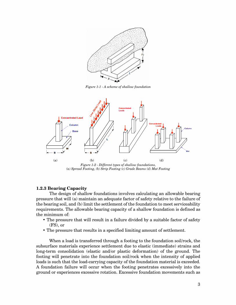
The definition of “shallow foundation” varies from author to author but generally is thought of as a foundation that bears at a depth less than about two times the foundation width (figure 1-1). Shallow foundations principally distribute structural loads over large areas of near-surface soil or rock to reduce the intensity of the applied loads to levels tolerable for the foundation soils. The definition is less important than understanding the theoretical assumptions behind the various design procedures. Stated another way, it is important to recognize the theoretical limitations of a design procedure that may vary as a function of depth, such as a bearing capacity equation.

Shallow foundations are used in many applications in highway projects when the subsurface conditions are appropriate. Such applications include bridge abutments on soil slopes or embankments, bridge intermediate piers, retaining walls, culverts, sign posts, noise barriers, and rest stop or maintenance building foundations. Footings or mats may support column loads under buildings. Bridge piers are often supported on shallow foundations using various structural configurations. Figure 1-2 presents an overall overview of different types of shallow foundations.

3

Figure 1-1 - A scheme of shallow foundation

Figure 1-2 - Different types of shallow foundations, (a) Spread Footing, (b) Strip Footing (c) Grade Beams (d) Mat Footing

1.2.3 Bearing Capacity

The design of shallow foundations involves calculating an allowable bearing pressure that will (a) maintain an adequate factor of safety relative to the failure of the bearing soil, and (b) limit the settlement of the foundation to meet serviceability requirements. The allowable bearing capacity of a shallow foundation is defined as the minimum of:

• The pressure that will result in a failure divided by a suitable factor of safety (FS), or

• The pressure that results in a specified limiting amount of settlement.

When a load is transferred through a footing to the foundation soil/rock, the subsurface materials experience settlement due to elastic (immediate) strains and long-term consolidation (elastic and/or plastic deformation) of the ground. The footing will penetrate into the foundation soil/rock when the intensity of applied loads is such that the load-carrying capacity of the foundation material is exceeded. A foundation failure will occur when the footing penetrates excessively into the ground or experiences excessive rotation. Excessive foundation movements such as

(a) (b) (c) (d)

4

penetration and rotation of the foundation may cause structural damage or collapse. A failure caused by the vertical and lateral displacement of foundation soils due to lack of sufficient strength is called a “bearing capacity failure” (figure 1-3). The load that develops this type of subsurface collapse is called the “ultimate bearing capacity” of the soil. Figure 1-5 presents a general scheme of finding bearing capacity methods according to the reliability, cost and range of use.

Figure 1-3 - Idealized axial load-displacement-capacity response of shallow foundations.

1.2.4 Allowable Bearing Capacity

The allowable bearing capacity of a spread footing historically has combined the design considerations of minimizing the potential for shear failure of the soil and limiting vertical deflection (settlement). Both of these design considerations are a function of the least footing dimension, typically called the “footing width,” and designated as the variable, B (figure 1-4). Generally, for a footing which is bearing on an isotropic, homogenous material, with no embedment (i.e., founded at the surface), the factor of safety against a failure developing beneath the footing will increase as the footing width, B, increases. However, as a footing’s dimension increases, the depth of influence also increases. Stated on another way, as the footing dimension, B, increases, the stress increase “felt” by the soil extends more deeply below the bearing elevation.

Figure 1-4 - Definition sketch of dimensions for a footing

5

Figure 1-5 - Methods for determining the bearing capacity of shallow foundations

1.2.5 Ultimate Bearing Capacity Ultimate bearing capacity, symbolized as qu, is the limiting load that a

foundation cannot exceed without causing failure within a soil mass. Evaluation of this ultimate bearing capacity is a difficult process as it is difficult to evaluate the shear strength parameters within the underlying soil structure.

After designing a foundation three types of failure mechanisms could occur when the ultimate bearing capacity is exceeded. The three failure mechanisms for a pad footing include; general shear failures, local shear failures and punching shear failures. Each of the three failure types has been discussed below in more details.

Experimental: - Full-load tests - Plate-load tests - Calibration chamber tests - Centrifuge tests

Numerical - Finite element programs (E.g. ABAQUS) - Finite difference programs (E.g. ANSYS, FLAC)

Analytical - Limit Equilibrium (e.g. Craig & Pariti, 1978; Atkinson, 1981) - Limit plasticity (e.g. Meyerhof, 1951, Terzaghi, 1943) - Cavity expansion (e.g. Skempton et al. 1951, Vesic, 1975)

Empirical - Schmertmann (1978) - Briaud (1995) - Clarke (1995)

Increasing use in practice

Bearing Capacity

Increasing reliability and cost

6

1.2.5.1 General Failure

The kinematic conditions (strain states) that develop when a uniform, rigid-plastic, weightless soil (possessing cohesion c' and friction φ') reaches the ultimate bearing capacity were determined theoretically by Prandtl (1920) and Reissner (1924). When a footing is loaded to the ultimate bearing capacity, the condition of plastic flow of foundation soils develops.

Terzaghi and Peck (1948) further defined the zones of plastic equilibrium after failure of soil beneath continuous footing (Figure 1-6). As shown in figure below, a triangular wedge beneath the footing, designated as Zone I, remains in an elastic state and moves down into the soil with the footing. Radial shear develops in Zone II such that radial lines extending from the footing change length based on a logarithmic spiral until the failure plane reaches Zone III. A passive state develops in Zone III at an angle of 45°

– (φ′/2) from the horizontal. This configuration of the

ultimate bearing capacity failure, with well-defined shear planes developing and extending to the surface, with bulging of the soil on both sides of the footing, is called “general failure”. General failure-type ultimate bearing capacity failures (Figure 1-7a) are believed to be the prevailing mode of failure for soils that are relatively incompressible and reasonably strong, or saturated, normally consolidated clays that are loaded rapidly so that undrained conditions and therefore undrained soil strength governs (Coduto, 1994).

Figure 1-6 - Boundaries of zone of plastic equilibrium after failure of

Soil Beneath Continuous Footing.

1.2.5.2 Local Failure

In some cases, the bearing capacity shear planes are not well developed, and the failure planes do not extend all the way to the ground surface. This mode of ultimate bearing capacity failure (Figure 1-7b) is called “local failure”. The deformation patterns in local shear involve vertical compression (Vesic, 1975) beneath the footing, swelling of the soil at the ground surface and essentially no rotation or tilting of the footing. Local failures may occur in soils that are relatively loose or soft when compared to soils susceptible to general failure.

7

1.2.5.3 Punching Failure

Another type of failure observed under ultimate bearing-capacity conditions involves vertical compression of the soils beneath the footing without bulging of the soil. As shown in figure 1-7c, the bearing load continuously increases when the footing is loaded under strain-controlled conditions (‘test at greater depth’). This kinematic mode of ultimate bearing capacity failure is called “punching failure”. Punching is considered as a potential failure mode for shallow foundations when loose or compressible soils are loaded slowly under drained conditions. For instance, footings placed at great depth on dense sand or on dense sand underlain by soft, compressible soil can fail under punching-shear modes. A footing on soft clay can also fail under punching shear if it is loaded slowly.

Figure 1-7 – Modes of bearing capacity failure (After Vesic, 1975)

The nature of failure in soil at ultimate load is a function of several factors such as the strength and the relative compressibility of the soil, the depth of the foundation (Df) in relation to the foundation width B, and the width-to-length ratio (B/L) of the foundation. This was clearly explained by Vesic, who conducted extensive laboratory model tests in sand. The summary of Vesic’s findings is shown in a slightly different form in figure 1-8. In this figure Dr is the relative density of sand, and the hydraulic radius R of the foundation is defined as: = Eq. 1-1

Where, A = area of the foundation = BL P = perimeter of the foundation = 2(B+L)

(a) General Failure

(b) Local Failure

(c) Punching Failure

Q

Q

Q

8

Thus, = ( ) Eq. 1-2

Figure 1-8 - Nature of failure in soil with relative density of sand Dr and Df/R.

From figure above it can be seen that when Df /R ≥ about 18, punching shear failure occurs in all cases irrespective of the relative density of compaction of sand. 1.2.6 Inclined Loading

The inclined load case is the resultant formed by both vertical and horizontal load components applied to the footing (figure 1-9). If the components of this resultant (i.e., axial and shear forces) are checked against the available resistance in the respective direction (i.e., bearing capacity and sliding, respectively). The bearing capacity should, however, be evaluated using effective footing dimensions, since large moments can frequently be transmitted to foundations by the columns or pier walls.

Unusual column geometry or loading configurations should be evaluated on a case-by-case basis relative to the foregoing recommendation to omit the load inclination factors. An example might be a support column that is not aligned normal to the footing bearing surface. In this case, it may be practical to consider an inclined footing base for improved bearing efficiency.

Figure 1-9 - A general scheme of shallow foundations with (a) Vertical loading (b) Inclined loading (both vertical and horizontal loading)

B B

V V

H

(a) (b)

α°

9

1.3 Research Objectives The modeling and analyzing of a shallow foundation close to a slope has some

difficulties and complexities. Since there are some terms and situations which need to be taken into consideration to evaluate completely the ultimate bearing capacity of a foundation. This project aims to make a model for shallow foundation adjacent to a slope to determine and analyze the behavior of soil, find the ultimate bearing capacity, make a comparison of numerical and theoretical values, and finally develop analytical solutions to find the bearing capacity and interaction locus. An overall scheme for this project can be observed within figure 1-10.

Figure 1-10 - Problem notation and potential failure mechanism.

The main objective of this project is simulating the conditions of figure 1-10

by taking advantages of the FLAC, in order to make a qualitative set of ultimate bearing capacity results for the soil structure underlying a shallow foundation. Before making this model, the simple situations for a shallow foundation, consisting of a shallow foundation with merely vertical loading and therefore a shallow foundation with both vertical and horizontal loading are modeled in order to make a logical comparison between the numerical results and theoretical values.

In modeling of these advanced models, an actual shallow foundation will be modeled in FLAC, in order to assess the foundation features. All results from these models will be validated and compared to existing solutions with the same properties and descriptions. 1.4 The Procedure

The project has been divided into many components to make it clear that it is successfully completed. These parts are as follows:

1. Research background information for the project. 2. Developing FLAC programming skills. 3. Producing the FLAC models for vertical and inclined loading with

different domain dimensions. 4. Producing the FLAC models for foundation near a slope under different

circumstances. 5. Validating the FLAC model results with previous solutions. 6. Developing the relevant solutions, charts and tables. 7. Concluding the thesis.

10

1.5 Chapters Overview This thesis provides a series of models for analysis of the foundation close to

a slope problem. The topics which are in this dissertation are; an introduction and background information into the project, a literature review of previous works, an introduction to FLAC, the development, validation and an advance study into the role of the interface between the base of the foundation and the underlying soil structure plays on the ultimate bearing capacity of the soil, with a series of equations, design charts and tables produced. Outlined below is a brief description of each chapter.

1.5.1 Chapter 1 – Introduction

This chapter presents the outline of the study, an introduction into the problem along with the essential background information for the problem and a discussion of the project's objectives and methodology. 1.5.2 Chapter 2 - Literature Review

This chapter will present a literature review of all previous studies on bearing capacity problems to introduce the project and give a background into why this study is required. Included within second chapter will be findings of past researchers, results from past dissertational FLAC modelling of the problem and finally an overview of the current available texts on the subject matter of shallow rigid foundations located on or near slopes. 1.5.3 Chapter 3 – Introduction to FLAC and Numerical Modeling

This chapter will present a brief introduction into the software that was used throughout this project. It will provide the abilities of the program together with, the methods used to simulate the project in the program. 1.5.4 Chapter 4 – The Results and Analysis

This chapter will present the results of advanced modellings of the interface between the soil structure and the base of the foundation. Within this chapter a validation of the numerical models will be conducted, along with the use of the model in the analysis of the interaction locus for a foundation overlying on different soils, for a range of different ratios of footing distance with slope edge and also slope angle. At the end, an analytical solution will be proposed to find the interaction domain of soil structure near the slope together with a proposed bearing capacity for stated problem. 1.5.5 Chapter 5 – Conclusion

This chapter will present the overall deductions from modelling studies presented within previous chapters. In addition this chapter will make a final conclusion on the status of previous studies that proposed to have constructed design charts and tables that conservatively calculated the ultimate bearing capacity for a rigid shallow foundation located near a slope, which can easily be used within preliminary foundation designs.

11

1.6 Summary

The objective of this chapter was to give the dissertation reader an introduction and a basic understanding of the content of the studies that are presented within this dissertation. From this chapter it is evident that there are many aspects that require consideration throughout the duration of this project. The following chapter presents the literature review of past studies that have been conducted within this project topic.

12

2. Literature Review

2.1 General In this chapter, a summary of previous researches that have been done and

published within geotechnical textbooks and journals, on the subject of “Ultimate bearing capacity” for a footing on flat ground condition and also sloped situation is presented. The extent of researches performed in this field with majority of the footings on a flat ground is not very wide.

During the past years, a number of researchers have done large amount of studies on shallow foundations and their ultimate bearing capacity. In this chapter, it is tried to present different theories of finding ultimate bearing capacity for foundations on flat ground and then sloped one that have been developed throughout the past years.

2.2 Previous Theories Finding a reliable value for bearing capacity of shallow footings was the aim

of lots of studies during the last century and has led to the development of various solutions. Full-scale load test are the most definitive means for determining the bearing capacity. After that, numerical analysis comes second to experimental processes in reliability and flexibility. It enables the user to properly model the site conditions (such as anisotropy, heterogeneity, variation of properties with depth boundaries). Also it makes it possible to observe the effects of changing the different parameters (e.g. groundwater table, footing dimensions, loading direction, boundary conditions). Nevertheless, numerical methods require specialized software skills. On the other side, empirical methods are characterized by simplicity but are usually limited in their applicability to specific test types. Conversely, analytical methods (e.g. limit equilibrium: Craig and Pariti, 1978; limit plasticity: Meyerhof, 1951; cavity expansion: Vesic, 1975) are more useful, thus making them more widely used in combination with a number of laboratory and in-situ tests. The classic analytical solutions for the bearing capacity are discussed below: 2.2.1 Bearing Capacity for Purely Vertical Loading

2.2.1.1 Terzaghi’s Bearing Capacity Theorem Karl von Terzaghi (1943) was the first to present a comprehensive theory for

the evaluation of the ultimate bearing capacity of rough shallow foundations under vertical loading. This theory states that a foundation is shallow if its depth is less than or equal to its width. Later investigations, however, have suggested that foundations with a depth, measured from the ground surface, equal to 3 to 4 times

13

their width may be defined as shallow foundations. Terzaghi developed a method for determining bearing capacity for the general failure case in 1943. Terzaghi’s equation utilized non-dimensional bearing capacity factors. Terzaghi’s theory was based on the theory of plasticity, which was a slight modification of a previous theory presented by Prandtl (1920), to analyze the punching effect of a rigid base into a softer soil material. The equations are given below. The original equation: = + + Eq. 2-1 Where, = ( ) Eq. 2-2 = ( − 1) Eq. 2-3 = tan − Eq. 2-4

Nc, Nq and Nγ = bearing capacity factors φ = soil friction angle c = soil cohesion Df = foundation depth B = foundation width γ = unit weight of soil Kpγ is obtained graphically. Simplifications have been made to eliminate the need for Kpγ. One such was done by Coduto [11], given below, and it is accurate to within 10%. = . Eq. 2-5

Table 2-1 shows different values of bearing capacity factors according to the

friction angle φ of soil. Kumbhojkar obtained the different values of Nγ.

Krizek suggested simple relations for bearing capacity factors of Terzaghi’s relation with a maximum deviation of 15% as follows: = . Eq. 2-6 = Eq. 2-7 = Eq. 2-8

Equations 2-2 to 2-4 are valid for frictions 0 to 35°. Terzaghi also proposed

two different equations for square and circular foundation: = 1.3 + + 0.4 (Square foundation, B×B) Eq. 2-9

And = 1.3 + + 0.3 (Circular foundation, B×B) Eq. 2-10

Based on numerous experimental studies, it deduced that Terzaghi’s

formulation and assumption for failure surface in soil at ultimate load is basically correct. However, the angle φ in figure 1-3 is closer to 45°+ (φ/2) and not φ, as

14

assumed by Terzaghi. In that case, the behavior of soil failure surface is shown in Figure 2-1.

Table 2-1. Terzaghi's Bearing Capacity factors - Equations 2-2, 2-3 and 2-4. φ Nc Nq Nγ 0 1 2 3 4 5 6 7 8 9

10 11 12 13 14 15 16 17 18 19 20 21 22 23 24 25 26 27 28 29 30 31 32 33 34 35 36 37 38 39 40 41 42 43 44 45 46 47 48 49 50

5.70 6.00 6.30 6.62 6.97 7.34 7.73 8.15 8.60 9.09 9.61 10.16 10.76 11.41 12.11 12.86 13.68 14.60 15.12 16.57 17.69 18.92 20.27 21.75 23.36 25.13 27.09 29.24 31.61 34.24 37.16 40.41 44.04 48.09 52.64 57.75 63.53 70.01 77.50 85.97 95.66 106.81 119.67 134.58 151.95 172.28 196.22 224.55 258.28 298.71 347.50

1.00 1.10 1.22 1.35 1.49 1.64 1.81 2.00 2.21 2.44 2.69 2.98 3.29 3.63 4.02 4.45 4.92 5.45 6.04 6.70 7.44 8.26 9.19

10.23 11.40 12.72 14.21 15.90 17.81 19.98 22.46 25.28 28.52 32.23 36.50 41.44 47.16 53.80 61.55 70.61 81.27 93.85 108.75 126.50 147.74 173.28 204.19 241.80 287.85 344.63 415.14

0.00 0.01 0.04 0.06 0.10 0.14 0.20 0.27 0.35 0.44 0.56 0.69 0.85 1.04 1.26 1.52 1.82 2.18 2.59 3.07 3.64 4.31 5.09 6.00 7.08 8.34 9.84

11.60 13.70 16.18 19.13 22.65 26.87 31.94 38.04 45.41 54.36 65.27 78.61 95.03

115.31 140.51 171.99 211.56 261.60 325.34 407.11 512.84 650.87 831.99 1072.80

15

Figure 2-1 - Modified failure surface in soil supporting a shallow foundation at ultimate load.

2.2.1.2 Meyerhof’s Bearing Capacity Theorem Meyerhof also published an additional theory in 1951 that could be applied

to rough, shallow and deep foundation. He considered a shape factor sq with the depth term Nq. He also considered the effect of shear resistance along the failure surface in the soil situated above the foundation (depth factors) and inclination factors during inclined loading that Terzaghi neglected to take into consideration. Figure 2-2 shows the failure surface at ultimate load under a continuous shallow foundation supposed by Meyerhof.

Figure 2-2 - Slip line fields for a rough continuous foundation.

In Figure 2-2, “abc” region represents the rigid wedge that was also shown in Figure 1-6, “bcd” is the radial shear zone with cd being an arc of log spiral, and “bde” is a mixed shear zone in which the shear varies between the limits of radial and plane shear depending on the depth and roughness of foundation. The “be” plane is called an equivalent free surface. The normal and shear stresses on plane be respectively are p0 and s0.

The produced equation by Meyerhof presented below: = + + Eq. 2-11 Where: qult = Soil bearing pressure (kPa).

c = cohesion of soil below foundation (kPa). B = width of footing Df = depth of footing

Nc, Nq, Nγ = bearing capacity factors.

16

2.2.1.2.1 Finding the Bearing Capacity Factors To find the bearing capacity factors, Meyerhof proposed the equations below. = ( ) Eq. 2-12 = − 1 Eq. 2-13

= − tan 45 + Eq. 2-14

Table 2-2 presents Meyerhof’s bearing capacity factors.

Table 2-2. Meyerhof’s Bearing capacity factors – Equations 2-11, to 2-13. φ Nc Nq Nγ 0 1 2 3 4 5 6 7 8 9 10 11 12 13 14 15 16 17 18 19 20 21 22 23 24 25 26 27 28 29 30 31 32 33 34 35 36 37

5.14 5.38 5.63 5.90 6.19 6.49 6.81 7.16 7.53 7.92 8.35 8.80 9.28 9.81

10.37 10.98 11.63 12.34 13.10 13.93 14.83 15.82 16.88 18.05 19.32 20.72 22.25 23.94 25.80 27.86 30.14 32.67 35.49 38.64 42.16 46.12 50.59 55.63

1.00 1.09 1.20 1.31 1.43 1.57 1.72 1.88 2.06 2.25 2.47 2.71 2.97 3.26 3.59 3.94 4.34 4.77 5.26 5.80 6.40 7.07 7.82 8.66 9.60 10.66 11.85 13.20 14.72 16.44 18.40 20.63 23.18 26.09 29.44 33.30 37.75 42.92

0.00 0.002 0.01 0.02 0.04 0.07 0.11 0.15 0.21 0.28 0.37 0.47 0.60 0.74 0.92 1.13 1.38 1.66 2.00 2.40 2.87 3.42 4.07 4.82 5.72 6.77 8.00 9.46 11.19 13.24 15.67 18.56 22.02 26.17 31.15 37.15 44.43 53.27

17

38 39 40 41 42 43 44 45 46 47 48 49 50

61.35 67.87 75.31 83.86 93.71 105.11 118.37 133.88 152.10 173.64 199.26 229.93 266.86

48.93 55.96 64.20 73.90 85.38 99.02

115.31 134.88 158.51 187.21 222.31 265.51 319.07

64.07 77.33 93.69

113.99 139.32 171.14 211.41 262.74 328.73 414.32 526.44 674.91 873.84

2.2.1.3 Hansen’s and Vesic’s Bearing Capacity Theorems After Meyerhof, Hansen (1970) developed his equation by considering base

factors for situations where we have tilted footing from horizontal. Although, Vesic (1973) established his own equation and bearing capacity by

conducting load tests on model circular foundations in sand, but it was based on Hansen’s equation. The different between the calculation of bearing capacity factors and inclination, base and ground factors are the different of these two theories. Table 2-3 and figure 2-3 give a comparison of Nγ values proposed by Terzaghi, Meyerhof, Vesic and Hansen.

Table 2-3. Comparison of Nγ Values for Shallow Foundation Nγ Soil Friction Angle φ (deg)

Terzaghi Meyerhof Vesic Hansen

0 1 2 3 4 5 6 7 8 9

10 11 12 13 14 15 16 17 18 19 20 21 22 23 24

0.00 0.01 0.04 0.06 0.10 0.14 0.20 0.27 0.35 0.44 0.56 0.69 0.85 1.04 1.26 1.52 1.82 2.18 2.59 3.07 3.64 4.31 5.09 6.00 7.08

0.00 0.002 0.01 0.02 0.04 0.07 0.11 0.15 0.21 0.28 0.37 0.47 0.60 0.74 0.92 1.13 1.38 1.66 2.00 2.40 2.87 3.42 4.07 4.82 5.72

0 0.07 0.15 0.24 0.34 0.45 0.57 0.71 0.86 1.03 1.22 1.44 1.69 1.97 2.29 2.65 3.06 3.53 4.07 4.68 5.39 6.2

7.13 8.2

9.44

0 0

0.01 0.02 0.05 0.07 0.11 0.16 0.22 0.3

0.39 0.5

0.63 0.78 0.97 1.18 1.43 1.73 2.08 2.48 2.95 3.5

4.13 4.88 5.75

18

25 26 27 28 29 30 31 32 33 34 35 36 37 38 39 40 41 42 43 44 45

8.34 9.84 11.60 13.70 16.18 19.13 22.65 26.87 31.94 38.04 45.41 54.36 65.27 78.61 95.03

115.31 140.51 171.99 211.56 261.60 325.34

6.77 8.00 9.46 11.19 13.24 15.67 18.56 22.02 26.17 31.15 37.15 44.43 53.27 64.07 77.33 93.69

113.99 139.32 171.14 211.41 262.74

10.88 12.54 14.47 16.72 19.34 22.4 25.99 30.22 35.19 41.06 48.03 56.31 66.19 78.03 92.25

109.41 130.22 155.55 186.54 224.64 271.76

6.76 7.94 9.32

10.94 12.84 15.07 17.69 20.79 24.44 28.77 33.92 40.05 47.38 56.17 66.75 79.54 95.05 113.95 137.1 165.58 200.81

Figure 2-3 - Comparison of Nγ Values for Shallow Foundation according to

Terzaghi, Meyerhof, Vesic and Hansen

2.2.1.4 Other Theories for Finding Bearing Capacity Lundgren and Mortensen [28] established numerical methods (using the

theory of plasticity) for the precise rupture lines determination as well as the bearing capacity factor for specific cases. Chen [9] also found a solution for Nγ by using the upper bound limit analysis theorem proposed by Drucker and Prager [14]. Biarez [6] also suggested the equation 2-15: = 1.8 − Eq. 2-15

Recently Kumar [33] suggested another slip line solution based on Lundgren

and Mortensen’s failure mechanism. Michalowski [37] also used the upper bound

0

5

10

15

20

25

30

35

40

45

50

0 50 100 150 200 250 300 350

Fric

tion

Angl

e (d

eg)

Nγ

TerzaghiMeyerhofVesicHansen

19

limit analysis theorem to obtain the variation of Nγ. His solution can be approximated as: = ( . . ) Eq. 2-16

Hjiaj et al. [34] obtained a numerical analysis solution for Nγ. This solution

can be approximated as: = ( )( ) Eq. 2-17 Martin [30] used the method of characteristics to achieve the variations of

Nγ. Salgado estimated these variations in the form: = − 1 tan(1.32 ) Eq. 2-18

Table 2-4 and Figure 2-4 provide and compare different values of Nγ obtained

by Chen, Booker, Kumar, Michalowski, Hjiaj et al., and Martin. The main reason that various values for Nγ were developed, is in the

difficulty of selecting a representative value of the soil friction angle φ for calculating bearing capacity. The parameter φdepends on many factors, such as intermediate principal stress condition, friction angle anisotropy, and curvature of the Mohr-Coulomb failure envelope.

Table 2-4. Comparison of Nγ Values for Shallow Foundation According to Chen, Kumar, Michalowski, Hjiaj et al. and Martin. Nγ Soil Friction Angle φ (deg)

Chen Kumar Michalowski Hjiaj et al. Martin

5 10 15 20 25 30 35 40 45

0.38 1.16 2.3 5.2 11.4 25 57

141 374

0.23 0.69 1.6

3.43 7.18

15.57 35.16 85.73

232.84

0.18 0.71 1.94 4.47 9.77

21.39 48.68

118.83 322.84

0.18 0.45 1.21 2.89 6.59 14.9 34.8 85.86

232.91

0.113 0.433 1.18 2.84 6.49

14.75 34.48 85.47

234.21

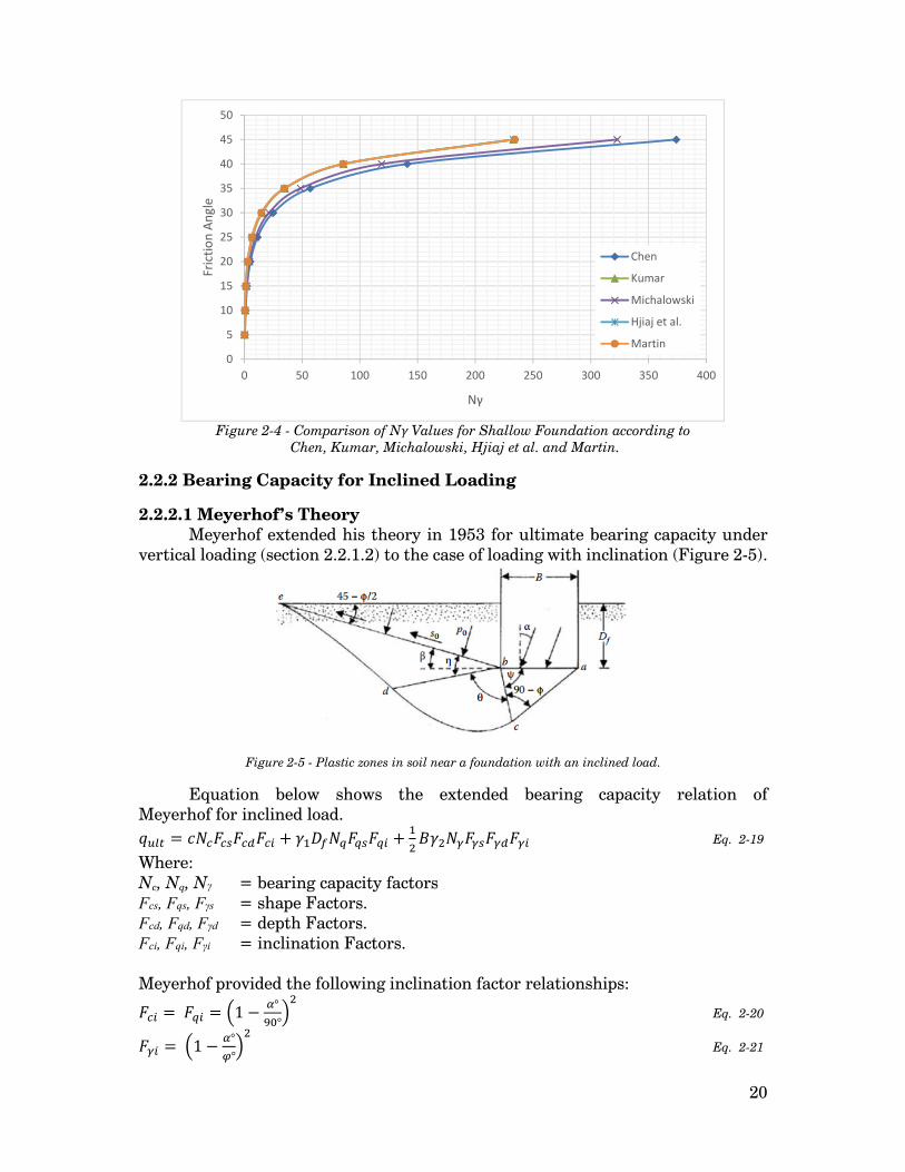
20

Figure 2-4 - Comparison of Nγ Values for Shallow Foundation according to

Chen, Kumar, Michalowski, Hjiaj et al. and Martin.

2.2.2 Bearing Capacity for Inclined Loading

2.2.2.1 Meyerhof’s Theory Meyerhof extended his theory in 1953 for ultimate bearing capacity under

vertical loading (section 2.2.1.2) to the case of loading with inclination (Figure 2-5).

Figure 2-5 - Plastic zones in soil near a foundation with an inclined load.

Equation below shows the extended bearing capacity relation of Meyerhof for inclined load. = + + Eq. 2-19

Where: Nc, Nq, Nγ = bearing capacity factors Fcs, Fqs, Fγs = shape Factors. Fcd, Fqd, Fγd = depth Factors. Fci, Fqi, Fγi = inclination Factors. Meyerhof provided the following inclination factor relationships: = = 1 − °° Eq. 2-20 = 1 − °° Eq. 2-21

0

5

10

15

20

25

30

35

40

45

50

0 50 100 150 200 250 300 350 400

Fric

tion

Angl

e

Nγ

Chen

Kumar

Michalowski

Hjiaj et al.

Martin

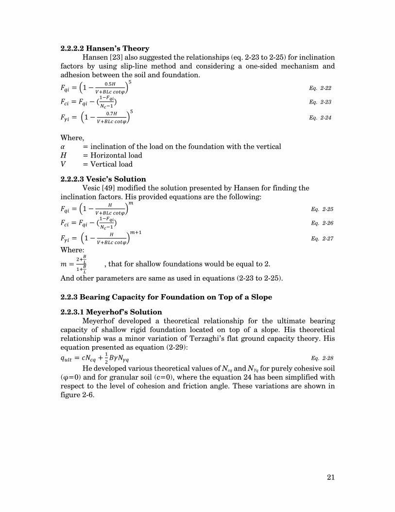
21

2.2.2.2 Hansen’s Theory Hansen [23] also suggested the relationships (eq. 2-23 to 2-25) for inclination

factors by using slip-line method and considering a one-sided mechanism and adhesion between the soil and foundation. = 1 − . Eq. 2-22 = − ( ) Eq. 2-23 = 1 − . Eq. 2-24

Where, α = inclination of the load on the foundation with the vertical H = Horizontal load V = Vertical load

2.2.2.3 Vesic’s Solution Vesic [49] modified the solution presented by Hansen for finding the

inclination factors. His provided equations are the following: = 1 − Eq. 2-25 = − ( ) Eq. 2-26 = 1 − Eq. 2-27

Where: = , that for shallow foundations would be equal to 2.

And other parameters are same as used in equations (2-23 to 2-25). 2.2.3 Bearing Capacity for Foundation on Top of a Slope

2.2.3.1 Meyerhof’s Solution Meyerhof developed a theoretical relationship for the ultimate bearing

capacity of shallow rigid foundation located on top of a slope. His theoretical relationship was a minor variation of Terzaghi’s flat ground capacity theory. His equation presented as equation (2-29): = + Eq. 2-28

He developed various theoretical values of Ncq and Nγq for purely cohesive soil (φ=0) and for granular soil (c=0), where the equation 24 has been simplified with respect to the level of cohesion and friction angle. These variations are shown in figure 2-6.

22

Figure 2-6 - Meyerhof’s bearing capacity factor,

(a) Ncq for purely cohesive soil and (b) Nγq for granular soil [13].

Where, Df is depth of footing, B is width of footing and β is slope angle.

2.2.3.2 Solution of Vesic and Hansen Whenever the foundation is located at the edge of the slope (b=0), the

solutions of Vesic and Hansen could be used. Hansen proposed a relationship for ultimate bearing capacity which shown in equation in (2-30): = + + Eq. 2-29

Where Nc, Nq, Nγ = bearing capacity factors (According to Table 2-3) λcβ, λqβ, λγβ = slope factors

q = γDf Referring to Hansen [23], = = (1 − ) Eq. 2-30 = ( > 0) Eq. 2-31 = 1 − ( = 0) Eq. 2-32

2.2.3.3 Limit Equilibrium and Limit Analysis Solution Based on Saran, Sud and Handa’s [41] examination which used the limit

equilibrium and limit analysis approach, we would have for a strip foundation, = + + Eq. 2-33

In the limit equilibrium approach, it is assumed that the footing is a shallow

strip footing having rough base and the soil above the base was replaced by an

(a) (b)

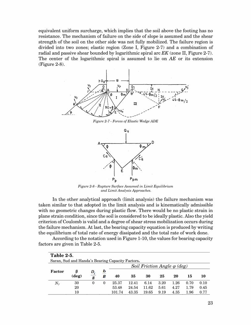
23

equivalent uniform surcharge, which implies that the soil above the footing has no resistance. The mechanism of failure on the side of slope is assumed and the shear strength of the soil on the other side was not fully mobilized. The failure region is divided into two zones; elastic region (Zone I, Figure 2-7) and a combination of radial and passive shear bounded by logarithmic spiral arc EK (zone II, Figure 2-7). The center of the logarithmic spiral is assumed to lie on AE or its extension (Figure 2-8).

Figure 2-7 - Forces of Elastic Wedge ADE

Figure 2-8 - Rupture Surface Assumed in Limit Equilibrium

and Limit Analysis Approaches.

In the other analytical approach (limit analysis) the failure mechanism was taken similar to that adopted in the limit analysis and is kinematically admissible with no geometric changes during plastic flow. There would be no plastic strain in plane strain condition, since the soil is considered to be ideally plastic. Also the yield criterion of Coulomb is valid and a degree of shear stress mobilization occurs during the failure mechanism. At last, the bearing capacity equation is produced by writing the equilibrium of total rate of energy dissipated and the total rate of work done.

According to the notation used in Figure 1-10, the values for bearing capacity factors are given in Table 2-5.

Table 2-5. Saran, Sud and Handa’s Bearing Capacity Factors. Soil Friction Angle φ (deg) Factor β

(deg)

40

35

30

25

20

15

10

Nγ 30 20 10

0

0

25.37 53.48

101.74

12.41 24.54 43.35

6.14 11.62 19.65

3.20 5.61 9.19

1.26 4.27 4.35

0.70 1.79 1.96

0.10 0.45 0.77

24

0 30 20 10 0 30 25 20

<15 30 25

<20

0 1 1

1

0

1

165.39 60.06 85.98

125.32 165.39 91.87

115.65 143.77 165.39 131.34 151.37 166.39

66.59 34.03 42.49 55.15 66.59 49.43 59.12 66.00 66.59 64.37 66.59 66.59

28.98 18.95 21.93 25.86 28.89 26.39 28.80 28.80 28.80 28.80 28.80 28.80

13.12 10.33 11.42 12.26 13.12

— — — — — — —

6.05 5.47 5.89 6.05 6.05 — — — — — — —

2.74 0.00 1.35 2.74 2.74 — — — — — — —

1.14 — — — — — — — — — — —

Nq 30 20

<10 30 20

<10

1 1

0

1

12.13 12.67 81.30 28.31 42.25 81.30

16.42 19.48 41.40 24.14 41.40 41.40

8.98 16.80 22.50 22.50 22.50 22.50

7.04 12.70 12.70

— — —

5.00 7.40 7.40 — — —

3.60 4.40 4.40 — — —

— — — — — —

Nc 50 40 30 20

<10 50 40 30 20

<10 50 40 30 20

<10 50 40 30

<20

0 0 0 1

0

1

0

1

21.68 31.80 44.80 63.20 88.96 38.80 48.00 59.64 75.12 95.20 35.97 51.16 70.59 93.79 95.20 53.65 67.98 85.38 95.20

16.52 22.44 28.72 41.20 55.36 30.40 35.40 41.07 50.00 57.25 28.11 37.95 50.37 57.20 57.20 42.47 51.61 57.25 57.25

12.60 16.64 22.00 28.32 36.50 24.20 27.42 30.92 35.16 36.69 22.38 29.42 36.20 36.20 36.20 35.00 36.69 36.69 36.69

10.00 12.80 16.20 20.60 24.72 19.70 21.52 23.60 27.72 24.72 18.38 22.75 24.72 24.72 24.72 24.72 24.72 24.72 24.72

8.60 10.04 12.20 15.00 17.36 16.42 17.28 17.36 17.36 17.36 15.66 17.32 17.36 17.36 17.36

— — — —

7.10 8.00 8.60 11.30 12.61

— — — — —

10.00 12.16 12.16 12.16 12.16

— — — —

5.50 6.25 6.70 8.76 9.44 — — — — — — — — — — — — — —

2.2.3.4 Stress Characteristics Solution As shown in Meyerhof’s equation (eq. 2-29), when the cohesion is equal to 0

(granular soils), the relationship would be: = Eq. 2-34

In this method, Graham, Andrews and Shields [22] presented a solution for finding the bearing capacity factor of shallow foundation adjacent to a slope edge, taking into account the stress condition immediately beneath the soil. In this method there is more accuracy in modeling the boundary and field condition for the failure mechanism in the soil. Also there would be a combination of different equation for stress transmission in plane-stress with Mohr-Coulomb relationship. Graham et al. considered the effect of progressive failure on the bearing capacity is negligible. Andrew suggested an adaptation of failure wedge of soil below the foundation. The shape and stress distribution of failure plane extended from the failure wedge were developed as the analysis proceeds and therefore, assuming the critical surface was not necessary. The strength is mobilized at the same time along

25

the potential failure plane at the ultimate load. The material considered isotropic. Works done by Andrew and Graham et al are shown in Figure 2-9 and Figure 2-10.

Figure 2-9 - Typical results after Andrew's procedures.

Figure 2-10 - Graham's asymmetric failure mechanism geometry [13]

A scheme of failure zone in the soil for embedment (Df/B) and setback (b/B) assumed for this approach is shown in Figure 2-11.

Figure 2-11 - A scheme of failure zones for embedment and setback: (a) Df/B > 0; (b) b/B > 0 [13]

Different values for Nγq gained from this procedure is given in following graphs (Figure 2-12).

26

Figure 2-12 - Graham, Andrews and Shields theoretical values of Nγq (Df/B=0) [22]

2.2.3.5 Other Solutions In 1981, Kusakabe et al. [27], developed an upper bound plasticity solution

to the vertical loading of footing on slopes. This method was the first to introduce the concept of the soil strength ratio and produced an empathetic of the soil strength relationship inside the slope.

Gemperline (1988) [17] developed an empirical solution for finding the bearing capacity factors. For this purpose, he used the results obtained from 215 centrifuge tests on a prototype slope model. According to 215 tests, he recommended a relationship for determining the bearing capacity factor Nγq, which used in Meyerhof’s equation for slopes. The Nγq could be found by equation below: = × × / × / × / , / × , / × , / , / × , / , / Eq. 2-35 Where, φ = angle of friction β = angle of slope B = foundation width b = distance from the top of slope D = embedded depth = 10( . . ) = 10( ) / = 1 + 0.65( / ) / = 1 − 0.27( / ) / , / = 1 + 0.39( / ) , / = 1 − 0.8[1 − (1 − ) ] 22 +

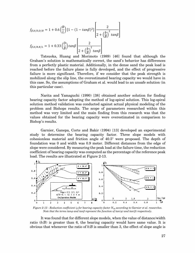
27

, / , / = 1 + 0.6 [1 − (1 − ) ] 22 +

, / , / = 1 + 0.33 22 +

Tatsuoka, Huang and Morimoto (1989) [46] found that although the Graham’s solution is mathematically correct, the sand’s behavior has differences from a perfectly plastic material. Additionally, in the dense sand the peak load is reached before the failure plane is fully developed, and the effect of progressive failure is more significant. Therefore, if we consider that the peak strength is mobilized along the slip line, the overestimated bearing capacity we would have in this case. So, the assumptions of Graham et al. would lead to an unsafe solution (in this particular case).

Narita and Yamaguchi (1990) [38] obtained another solution for finding bearing capacity factor adopting the method of log-spiral solution. This log-spiral solution method validation was conducted against actual physical modeling of the problem and Bishops results. The scope of parameters researched within this method was very limited and the main finding from this research was that the values obtained for the bearing capacity were overestimated in comparison to Bishop’s results.

Garnier, Ganepa, Corte and Bakir (1994) [13] developed an experimental

study to determine the bearing capacity factor. Three slope models with cohesionless material and friction angle of 40.5° were proposed. The depth of foundation was 0 and width was 0.9 meter. Different distances from the edge of slope were considered. By measuring the peak load at the failure time, the reduction coefficient of bearing capacity was computed as the percentage of the reference peak load. The results are illustrated at Figure 2-13.

Figure 2-13 - Reduction coefficient iβ for bearing capacity factor Nγq according to Garnier et al. researches.

Note that the terms tanφ and tanβ represent the function of tan(φ) and tan(β) respectively.

It was found that for different slope models, when the value of distance/width ratio (b/B) is greater than 6, the bearing capacity would have same value. It is obvious that whenever the ratio of b/B is smaller than 3, the effect of slope angle is

28

very significant and by considering the footing at the edge of slope, the reduction varies nearly linearly with respect to tan(β).

The equations below propose the reduction coefficient for bearing capacity of foundations near a slope: = 1 − [1.8 ° − 0.9 tan °](1 − ) for b/B<6 Eq. 2-36 = 1 for b/B>6

Georgiadis et al. (2008) proposed a finite element analysis for a footing close to a slope or on undrained soil slopes. This approach was able to consider the undrained bearing capacity factor, footing distance ratios, footing height ratios, the slope height and the soil properties and behaves as many of the available methods of evaluation the bearing capacity.

Catherine Smith [45], Joshua Watson [50] and Nathan Lyle [29] conducted different studies using the numerical modelling program called Fast Lagrangian Analysis of Continua or FLAC. These studies focused on numerous geotechnical problems including the problem of a foundation on top of a slope for a number of different problems. Catherine Smith considered a cohesionless soil and parameters considered were the slope angle, footing distance ratio and the dimensionless strength ratio. The primary outputs of this research were that the numerical modeling program, FLAC, was producing acceptable results according to theoretical bearing capacity values, when the number of elements and mesh size used to model the problem was reduced. Joshua Watson developed a research to find out the effects of several of non-dimensional parameters and different modeling methods for bearing capacity on top of a slope. The effect of the footing distance ratio, the footing height ratio, footing length ratio, the effect of the interface between foundation and foundation material were conducted within this research. Also an analysis of large deformation with respect to small deformation were done in this project. Nathan Lyle further worked on the researches of Joshua Watson and developed it by conducting more comprehensive studies into the shallow foundation located near a purely cohesive slope. Nathan conducted a wider range of parametric studies for analyzing the ultimate bearing capacity. It was determined that the results obtained in this research were approximately 10 percent higher than the upper bound solution produced by Shiau et al., therefor, the accuracy was in an acceptable range. 2.2.4 Horizontal Bearing Capacity

The mentioned solutions in the last part were for the case that only the vertical loading is present. Nevertheless, in the case of inclination of loading, the failure might occurs by sliding of the foundation along its base or by general shear of the soil. Many methods are produced for finding the horizontal bearing capacity and in almost all of them, horizontal bearing capacity has a relationship with the vertical bearing capacity. The following equation is proposed for finding the horizontal bearing capacity by lots of authors: = + Eq. 2-37

29

Where, c = cohesion of the soil φ = friction angle

Butterfield (1988) used the experimental results of Meyerhof (1963) [33], Hansen (1970) [23], Muhs and Weiss (1973) [13] and Vesic (1975) [13] on sand beds with different densities and on Brass-rod models with footings covering a wide range of sizes and proposed that the maximum horizontal load is equal to about 0.12 of maximum vertical load. His researches are presented in the Figure 2-14:

Figure 2-14- Comparison of Different Horizontal Bearing Capacities presented by Butterfield.

Figure 2-14 shows that almost in all of the cases, the maximum horizontal load occurs near the Vmax/2. The initial slope of the diagram is equal to tan(φ) and it depends on the surface sliding of the foundation.

2.3 Interaction Locus of Bearing Capacities 2.3.1 Interaction Locus of Horizontal Ground

At the previous part, the methods for finding and estimating the vertical and horizontal bearing capacity were presented. Despite the fact that all the mentioned solutions are popular due to their simplicity, but it can be observed that they are not very accurate to find the bearing capacities for vertical, inclined or eccentric loading. Since linear elasticity implies that the effect of each loading component is considered independently and therefore, the total displacement pattern can be obtained by superposition. Nevertheless, the experimental tests show that the displacement components are dependent to each other. Hence, it is evident that a combination of Vertical, Horizontal and Moment loading in the shape of failure envelope is needed. These envelopes have been produced by numerous authors through physical experiments, finite element analysis and limit state theorems.

Ticof [48] was the first one presenting an idea of combination of vertical and horizontal loads causing failure of a foundation overlying on sand, on a simple parabolic curve. He also proposed a similar parabolic curve for vertical load and moment. He introduced a three-dimensional surface with (V, H, M/B) axes which have geometrically similar elliptic cross sections in all planes where V

30

is constant (0<V<Vmax) and their major and minor axes lying the V-H and V-M/B planes respectively and intersecting all planes passing through the V axis in parabolic curves. The formula proposed by Ticof for these curves is shown below: = ( ) Eq. 2-38

Where, Vmax = central vertical load capacity of foundation th = soil friction coefficient

Figure 2-15 shows the two and three dimensional interaction locus between horizontal loading and momentum vs vertical loading.

Figure 2-15 - Interaction Locus of (a) Horizontal Bearing Capacity vs Vertical Bearing Capacity, (b) Horizontal

Bearing Capacity and Momentum vs Vertical Bearing Capacity , proposed by Ticof

Montrasio and Nova [39] presented a mathematical model with two hypothesis of: (a) the foundation is rigid and can be considered as a macro-element with the soil (loads of V, H and M as generalized stress and displacements and rotations as strain variables). (b) The constitutive law of macro-element, the relationship between generalized stress and strain, is considered rigid-plastic strain-hardening with non-associated flow rule. This model was built by using experimental results.

Nova presented the following equation for V-H parabola: ( , , ) ≡ − 1 − = 0 β=0.95 Eq. 2-39

Where: β = shape factor μ = friction coefficient

According to the equations above when V is much smaller than Vmax the first equation becomes H=μV. Butterfield [3] found out that the maximum H load capacity is developed, as predicted, when V=Vmax/2 and its value is Hmax ≅ Vmax/8 that is corresponding to μ=0.5.

31

Gottardi [3] have established the shape of the failure envelope in the (M/B-H) plane to be an ellipse (axis ratio R = 1.64) rotated through an angle ρ=13° from the H axis towards the + M/B axis. Figure 2-16 shows their best fit elliptical cross-section through failure points obtained from loading tests lying in the V=constant=Vmax/2 plane.

Figure 2-16 - Interaction Locus of Horizontal Loading vs. Moment

The data of the Figure 2-16 came from high-quality model tests on rough, rigid, dense-sand supported, surface foundations reported by Ticof [48], Butterfield and Gottardi [3]. In Butterfields’ tests the application of the load on the foundation base was done by applying constant velocity; all the other tests were load-controlled. Gottardi and Butterfield [3] performed a wide range of load paths to failure and proved that the failure envelope was essentially load-path independent. This inclined ellipses three-dimensional failure envelope was defined by: + − = ( )

Eq. 2-40

Where: th = 0.52 tm = 0.35 C = 0.22 Also a normalized version of the equation above was introduced: + − = ( (1 − )) Eq. 2-41

Where: r = V/Vmax m’ = M/BVmax n’ = H/Vmax

For designing foundations, this equation is probably the most convenient way to explore the safety of specific combinations of (n’, m’, r) and the consequences of changing any of them (Butterfield, 1993).

32

By defining n”=n’/th and m”=m’/tm the equation 2-42 becomes to following

relationship: ( ") + ( ") − 2 " " = ( (1 − )) Eq. 2-42 In equation above, when m”=0 (i.e. only vertical and horizontal loading), we

have n”=r (1-r), and when n”=0 (i.e. only vertical and moment loading), we have m”=r (1-r). The results from all the tests of this kind place on a single parabola which intersects the V axis at 45° and has a maximum central ordinate of 0.25. Figure 2-17 shows the data for all H = 0 and M = 0 loading tests:

Figure 2-17 - Interaction Locus for Simplified Vertical Load vs. Horizontal Load, or Moment.

By dividing the equation 2-42 to (r (1-r)) 2, it becomes to: + − 2 = 1 Eq. 2-43

The results from simple V-H for m=0, and V-(M/B) for n=0 loading now

reduce to n=m=1. Figure 2-18 is demonstrating the n-m plot for experimental points, for the least-squares best-fit ellipse which has an axis ratio 2 of 1.22 (corresponding to C = 0.20) and ρ = 44°.

Figure 2-18 - Best fit Ellipse for Normalized "n-m" Plot

All of the presented formulas demonstrate that for achieving a safe design for the shallow foundation under load increments, the design vertical load should be about Vmax/2; since these foundations are vulnerable to horizontal load and moment increments, and they can be brought to failure when H reaches Vmax/8 or

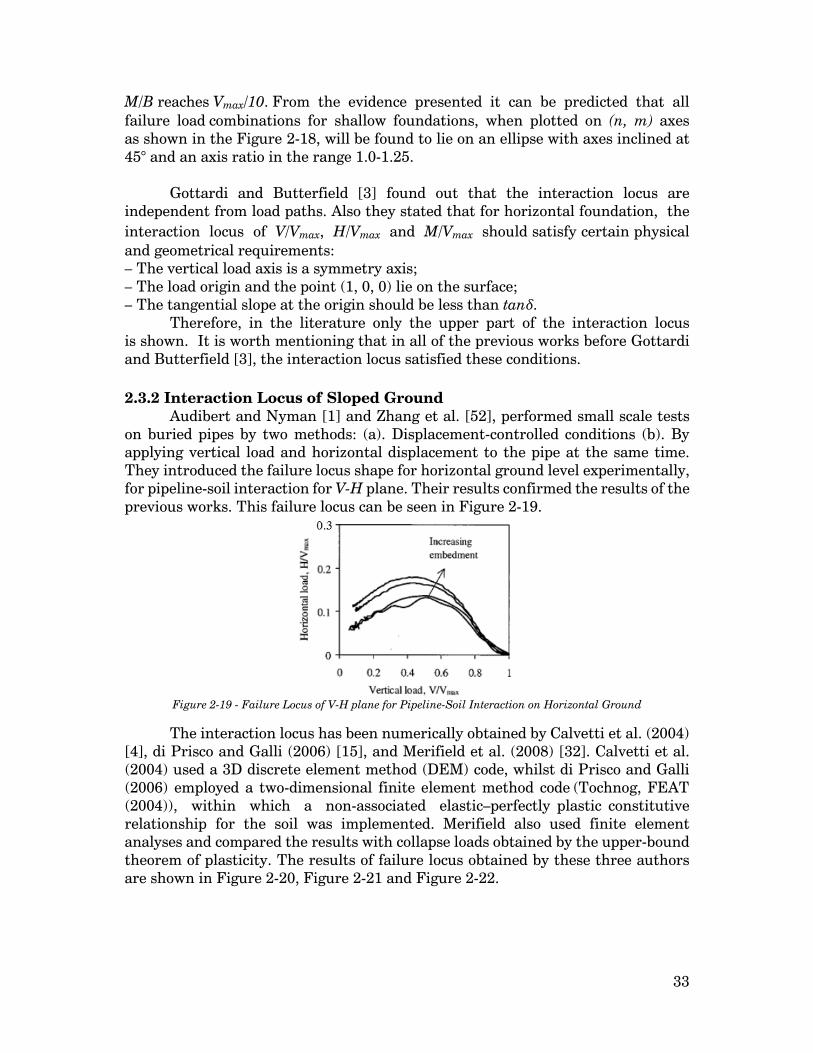
33

M/B reaches Vmax/10. From the evidence presented it can be predicted that all failure load combinations for shallow foundations, when plotted on (n, m) axes as shown in the Figure 2-18, will be found to lie on an ellipse with axes inclined at 45° and an axis ratio in the range 1.0-1.25.

Gottardi and Butterfield [3] found out that the interaction locus are independent from load paths. Also they stated that for horizontal foundation, the interaction locus of V/Vmax, H/Vmax and M/Vmax should satisfy certain physical and geometrical requirements: – The vertical load axis is a symmetry axis; – The load origin and the point (1, 0, 0) lie on the surface; – The tangential slope at the origin should be less than tanδ.

Therefore, in the literature only the upper part of the interaction locus is shown. It is worth mentioning that in all of the previous works before Gottardi and Butterfield [3], the interaction locus satisfied these conditions. 2.3.2 Interaction Locus of Sloped Ground

Audibert and Nyman [1] and Zhang et al. [52], performed small scale tests on buried pipes by two methods: (a). Displacement-controlled conditions (b). By applying vertical load and horizontal displacement to the pipe at the same time. They introduced the failure locus shape for horizontal ground level experimentally, for pipeline-soil interaction for V-H plane. Their results confirmed the results of the previous works. This failure locus can be seen in Figure 2-19.

Figure 2-19 - Failure Locus of V-H plane for Pipeline-Soil Interaction on Horizontal Ground

The interaction locus has been numerically obtained by Calvetti et al. (2004) [4], di Prisco and Galli (2006) [15], and Merifield et al. (2008) [32]. Calvetti et al. (2004) used a 3D discrete element method (DEM) code, whilst di Prisco and Galli (2006) employed a two-dimensional finite element method code (Tochnog, FEAT (2004)), within which a non-associated elastic–perfectly plastic constitutive relationship for the soil was implemented. Merifield also used finite element analyses and compared the results with collapse loads obtained by the upper-bound theorem of plasticity. The results of failure locus obtained by these three authors are shown in Figure 2-20, Figure 2-21 and Figure 2-22.

34

Figure 2-20 - Failure Locus of V-H Plane for Pipeline-Soil Interaction by Calvetti et al.

Figure 2-21 - Failure Locus for V-H plane for Pipeline-Soil Interaction by di Prisco & Galli

Figure 2-22 - Failure Locus for V-H Plane for Pipeline-Soil Interaction by Merifield et al.

The shape of interaction locus is dependent on geometrical boundary conditions such as embedment, slope inclination, and pipe-axis orientation with respect to the slope. Di Prisco et al. (2004) showed that for a pipe positioned in a homogeneous purely cohesive soil stratum characterized by a constant value of the undrained strength Su, by employing a simplified approach based on limit analysis, the interaction locus in the V–H plane progressively gets a circular shape, i.e., at increasing relative depths z/D, failure mechanisms become progressively similar in all directions, and the system response tends to become isotropic. This is shown in Figure 2-23.

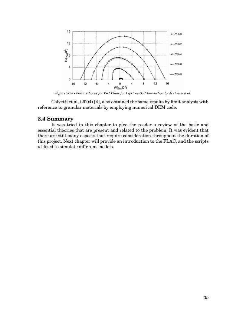
35

Figure 2-23 - Failure Locus for V-H Plane for Pipeline-Soil Interaction by di Prisco et al.

Calvetti et al, (2004) [4], also obtained the same results by limit analysis with reference to granular materials by employing numerical DEM code. 2.4 Summary

It was tried in this chapter to give the reader a review of the basic and essential theories that are present and related to the problem. It was evident that there are still many aspects that require consideration throughout the duration of this project. Next chapter will provide an introduction to the FLAC, and the scripts utilized to simulate different models.

36

3. Introduction to FLAC

and Numerical Modeling

3.1 Introduction

Within this chapter, an overview of the code FLAC (Fast Lagrangian Analysis of Continua) is presented. The program was used throughout this thesis to model and analyze the problem of shallow foundation on top of a slope. The following chapter is an explanation of the program and its features, the methods and scripts used to model and analyze the problem, along with numerical modeling procedures to assess the bearing capacity. 3.2 Fast Lagrangian Analysis of Continua

“FLAC is a two-dimensional explicit finite difference program for engineering mechanics computation”, referring to Itasca [24]. This program is able to model engineering structures on various geotechnical soil materials, such as soil, rock or similar materials, to investigate the behavioral effects of plastic flow within the material after a yield limit has been reached. FLAC uses a time stepping procedure rather than forming a stiffness matrix like finite element solutions, since it is an explicit finite difference program.

FLAC offers large strain simulation of continua, using interfaces that simulate faults, joints or boundaries, driven by an explicit solution scheme that can model unstable physical processes. It offers fourteen built-in material models, groundwater flow, coupled mechanical-flow calculation, inclusion of structural elements, plotting statistical distribution of any property, optional automatic remeshing during solution and a built-in scripting language (FISH) to customize or automate virtually all aspects of program operation, including user-defined properties and other variables.

Various number of FLAC versions are available now, with the most current version being 7.00. Nevertheless, throughout this dissertation the version 5.00 is used, due to its availability. According to Nathan Lyle [29], the difference between the two versions was only the marginal, and the newer version contained a number of different speed improvements. Therefore, the use of version 5.00 over version 7.00 would not compromise the accuracy of all advanced modeling solutions presented within this dissertation.

37

3.2.1 Key Features of FLAC According to Itasca’s program explanation, the program had a number of

major features that were utilized within this project. These features listed as: 1. Large-Strain simulation of continua, with the optional interface option that

simulated distinct planes along which slip and/or separation can occur. 2. Explicit solution scheme, giving stable solutions to unstable physical processes. 3. Groundwater flow, with full coupling to mechanical calculations (including

negative pore pressure, unsaturated flow and phreatic surface calculations). 4. Convenient specifications of general boundary conditions. 5. Library of material models (e.g. Mohr-Coulomb plasticity, ubiquitous joint,

double-yield, strain-softening, modified Cam-Clay and Hoek-Brown). 6. Automatic re-meshing during the solution process in large strain simulations. 7. Pre-defined database of material properties; users may add and save their own

material properties specifications to the database. 8. Statistical distribution of any property with extensive facility for generating

plots of virtually any problem variable. Despite the fact that FLAC has the mentioned features, in order to simulate the numerical models, features number 1, 4, 6, 7 and 8 are used. 3.3 Problem Definition

In the entire history of foundation designing, the difficulty of finding the bearing capacity of a shallow foundation near a slope has been an issue for lots of engineers, and therefore initiated numerous researches on influence of different parameters (such as soil properties, foundation size, soil volume dimensions, slope angle, distance ratio and etc.) on the bearing capacity and interaction domain. The most part of works done recently was about finding the ultimate bearing capacity of a foundation on horizontal ground, along with interaction domain of horizontal and vertical bearing capacity. Nevertheless, there is still lots of free spaces about the interaction domain of foundation near the slope. The main objective of this dissertation is to fulfill some of these free spaces by modeling and testing different situation for two kinds of soils; loose and dense sand, together with comparing to theoretical solutions. For this purpose, a two meter wide strip foundation has been modeled in FLAC and by trial and error using, the optimum cases for soil volume dimensions, applying force velocity and meshing size is found. 3.4 Producing Numerical Models within FLAC

Presented in this dissertation are the modeling and analysis of different situations that affect the interaction locus of horizontal and vertical bearing capacity. The parameters α°, β°, γ, φ°, ψ°, c and b/B (referring to Figure 1-9) are the input data of finite element model. Nine load inclination with the vertical (α°) equal to 0°, 6°,11°, 18° and 30° were considered. Correspondingly three slope models with β° equal to 10°, 20° and 30° have been modeled. The case of 0° was taken as the case of foundation on surfaced ground. For each slope model, the footing was placed in different locations in horizontal direction. This location was based on the b/B ratio, which was assigned to be equal to 0, 0.5, 1, 2 and 4. The variation of the ultimate

38

bearing capacity with respect to the location of footing in horizontal direction and also angle of slope can be observed. All the mentioned variations are used for both loose and dense sand with different γ, φ° and ψ°. In this investigation a total of 328 tests were performed (also considering the trial and error tests done for calibrations).

But before that, some preliminary studies and trial and error would be performed in order to find the optimum set of parameters of model. Each model was based on the adaptations of a simplified code produced by previous studies conducted within this area of study. Presented below are the basic steps that have been undertaken within the FLAC model, to analyze the shallow foundation located near a slope: 3.4.1 Making Geometry

1. The first step is to define various input variables for the model. 2. The subsequent step is to specify the magnitude of the gravity. 3. Forwarding step is to define the properties of soil mesh and the foundation

structure meshing. 4. The fourth step is to set up the extents and boundaries of the model. 5. The next step in to apply the initial stresses. For this purpose, the command

“solve” is used at the end of fourth step. The mentioned steps are shown in Figure 3-1:

Figure 3-1 - The first five steps before applying the loading to the model

To set up the initial finite difference grid, the “grid” command is used. The commands used in Figure 3-1 will produce an initial grid that is 40 by 24 zones for width and depth respectively. Therefore, by using “gen”, the coordinates and the size of domain will be produced. Afterward, the gravity by typing “set gravity=9.81” has been set, where 9.81 m/s2 is the acceleration due to gravity. Then, properties of material were defined in the model. Constitutive laws in FLAC are defined utilizing command “model”. The Mohr-Coulomb failure criterion (Figure 3-2) of elasto-plastic constitutive law is used in this project.

39

Figure 3-2 - Mohr-Coulomb Failure Criterion.

As mentioned before, two types of soil are modeled in this dissertation, whose their mechanical parameters are presented below in table 3-1.

Table 3-1. Soil properties used in this dissertation. Properties

Type Mass Density (kg/m3)

Friction φ

(°)

Cohesion c

(kPa)

Bulk Modulus

(kPa)

Shear Modulus

(kPa)

Dilation ψ (°)

Loose Sand

Dense Sand

1600

2000

35

40

0

0

1.67E7

5.56E7

1E7

4.17E7

0

10

The angle of dilation (Figure 3-3) controls the amount of volumetric strain developed during plastic shearing and is assumed constant during plastic yielding. The value of ψ=0 corresponds to the plastic volume preserving deformation while in shear. Clays (regardless of over consolidated layers) are characterized by a very low amount of dilation (ψ≈0).

Soils dilate (expand) or contract upon shearing and the degree of this dilatancy can be explained by the dilatancy angle, ψ.

Figure 3-3 - The element is dilating during shear. This plastic behavior.

(Referring to Salgado, the Engineering of Foundations)

40

Subsequently the boundary conditions for the problem are set. The boundary points of sides and bottom of domain should be fixed, hence by using “fix” command, the boundaries mentioned are fixed then.

The unbalanced force indicates when a mechanical equilibrium state (or the onset of plastic flow) is reached for a static analysis. A model is in exact equilibrium if the net nodal force vector at each grid point is zero. The maximum nodal force vector is monitored in FLAC and printed to the screen when the “solve” or “cycle” command is invoked. The maximum nodal force vector is also called the unbalanced or out-of-balance force. The maximum unbalanced force will never exactly reach zero for a numerical analysis. The model is considered to be in equilibrium when the maximum unbalanced force is small compared to the total applied forces in the problem. If the unbalanced force approaches a constant nonzero value, this probably indicates that failure is occurring within the model.

The “solve” function is used to apply the initial stresses along Y and X direction. In order to compare the initial stresses with the theoretical solution, the equation below is performed: = Eq. 3-1 = Eq. 3-2 = Eq. 3-3

Where, γ = mass density of soil (kg/m3) Z = depth of soil domain g = ground acceleration (9.81 m/s2) K0 = horizontal stress coefficient = Poisson’s ratio

The Figure 3-4 shows a scheme of initial stresses applied to the model after

the preliminary steps (Making Geometry part):

41

Figure 3-4 - The initial stress along Y direction.

It can be observed from figure 3-4 that the initial stress at the bottom of soil volume is about 90.00 kPa. Table 3-2 presents an example of the value of theoretical solution for scripts shown in Figure 3-1 with the dimensions that modeled:

Table 3-2. Computing the theoretical initial Stress. Properties Results

Equation Mass Density (kg/m3)

Depth

(m)

Ground Acceleration

(m/s2)

Effective Stress (kPa)

Error

(%) = 1600 6 9.81 94.2 4.43

It must be mentioned that this project and its values in the program are

based on “Metric System (SI)”. Hence, the dimensions are defined in “meter (m)” and stresses are defined in “Pascal (Pa)”. 3.4.2 Applying Loads

After performing preliminary parts and modeling the first part of problem, the next step is applying the initial velocities at the base of foundation to signify the presence of the foundation. Afterwards, the effects they have on the soil structure can be investigated. The final step is to save the graphical and numerical output data that is produced during the solution phase of the FLAC model.

A summation of maximum vertical and horizontal loads are necessary to compute the vertical and horizontal bearing capacity. Therefore the parameters “vload” (referring to vertical loads) and “hload” (referring to horizontal loads) are defined to sum up all the vertical and horizontal loads. (Figure 3-6 part (a) and (b)).

Z

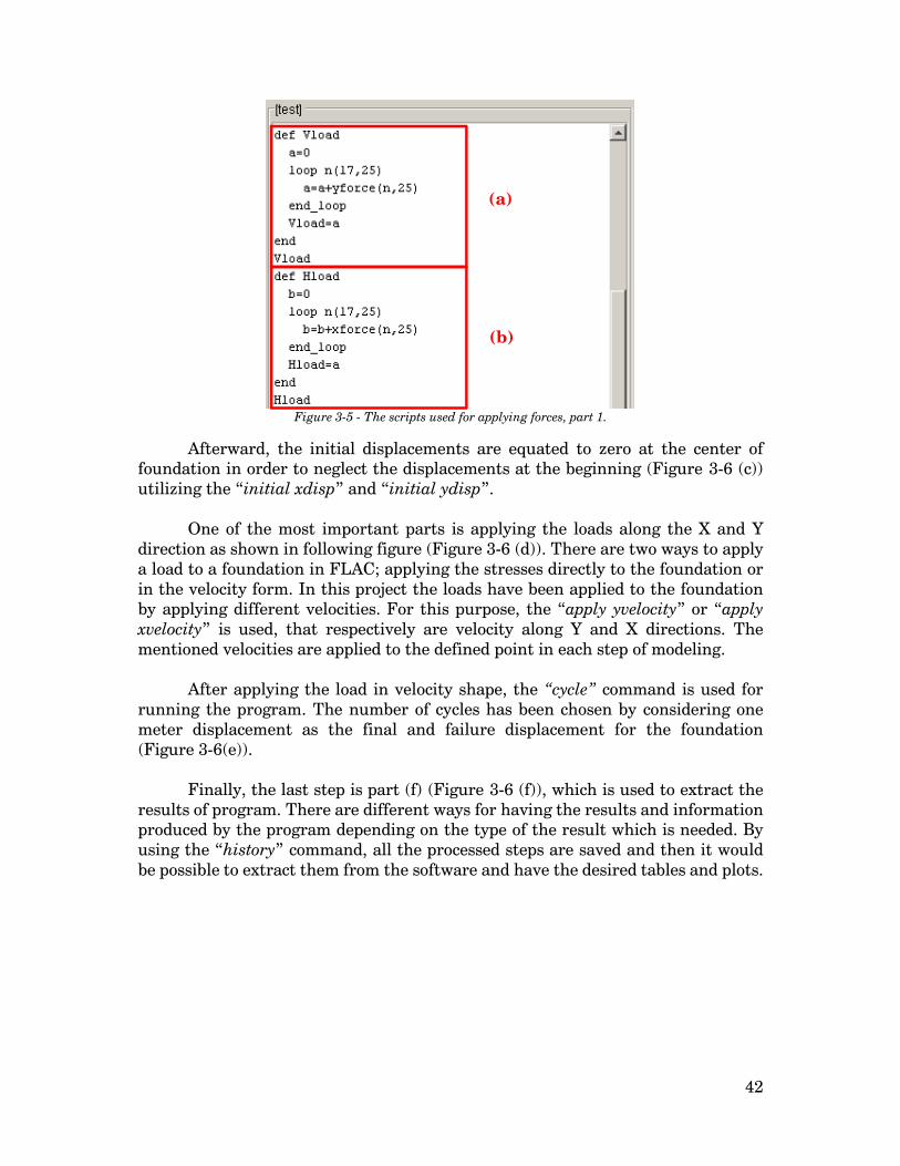
42

Figure 3-5 - The scripts used for applying forces, part 1.

Afterward, the initial displacements are equated to zero at the center of foundation in order to neglect the displacements at the beginning (Figure 3-6 (c)) utilizing the “initial xdisp” and “initial ydisp”.

One of the most important parts is applying the loads along the X and Y

direction as shown in following figure (Figure 3-6 (d)). There are two ways to apply a load to a foundation in FLAC; applying the stresses directly to the foundation or in the velocity form. In this project the loads have been applied to the foundation by applying different velocities. For this purpose, the “apply yvelocity” or “apply xvelocity” is used, that respectively are velocity along Y and X directions. The mentioned velocities are applied to the defined point in each step of modeling.

After applying the load in velocity shape, the “cycle” command is used for

running the program. The number of cycles has been chosen by considering one meter displacement as the final and failure displacement for the foundation (Figure 3-6(e)).

Finally, the last step is part (f) (Figure 3-6 (f)), which is used to extract the

results of program. There are different ways for having the results and information produced by the program depending on the type of the result which is needed. By using the “history” command, all the processed steps are saved and then it would be possible to extract them from the software and have the desired tables and plots.

(a)

(b)

43

Figure 3-6 - The scripts used for applying forces, part 2.

The Figure 3-7 shows an example of the simulated model that is produced by the mentioned commands and scripts.

Figure 3-7 - A model produced by using the indicated codes.

3.4.3 Modeling the Slopes

Processing the slope models are similar to horizontal ground situation described in previous part, nevertheless the following codes is added to the main script (Figure 3-8):

(d)

D=

6m

(f)

(c)

(e)

B=2m

W=10m

44

Figure 3-8 - The supplementary part of the scripts for modeling the slope.

Presented script in figure above (Figure 3-8) is the part that make the possibility of changing the slope angle and footing distance from the edge of slope. Figure 3-9 presents the output model of the slope coded in figure 3-8:

Figure 3-9 - A sloped model produced by using the supplementary codes.

In the following, a scheme of simulated models is presented to show the geometry of various models with various variables of b and β and also different situation of load applying by different load inclinations(α):

D=

15m

W=25m

D=

11.5

4m

β=20° B=2m b=2m

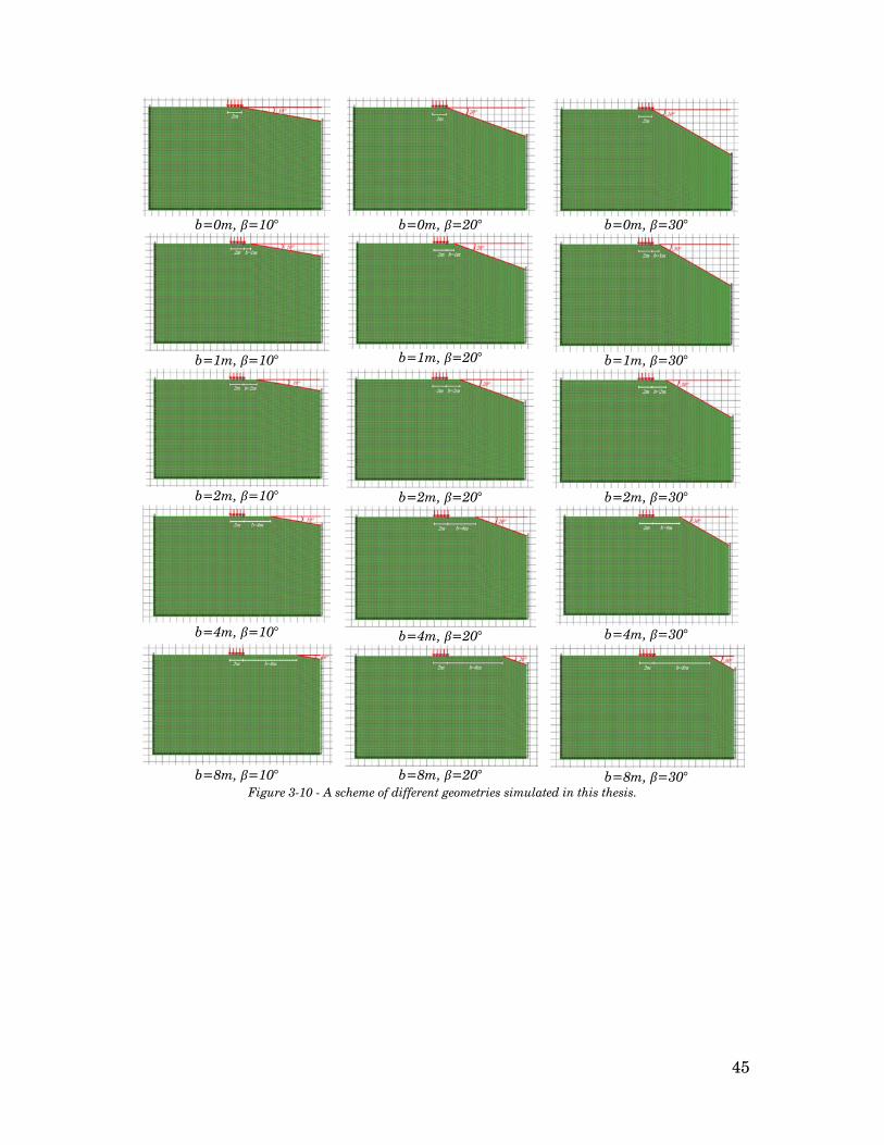
45

b=0m, β=10°

b=0m, β=20°

b=0m, β=30°

b=1m, β=10°

b=1m, β=20°

b=1m, β=30°

b=2m, β=10°

b=2m, β=20°

b=2m, β=30°

b=4m, β=10°

b=4m, β=20°

b=4m, β=30°

b=8m, β=10°

b=8m, β=20°

b=8m, β=30°

Figure 3-10 - A scheme of different geometries simulated in this thesis.

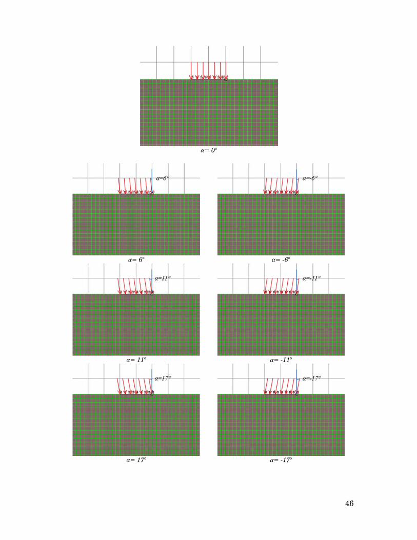
46

α= 0°

α= 6°

α= -6°

α= 11°

α= -11°

α= 17°

α= -17°

47

α= 30°

α= 30°

Figure 3-11 - A scheme of different loading cases simulated in this thesis.

3.5 Running the Model In order to find the final domain dimensions, velocity of loading and optimum size of elements, different tests are modeled and by using trial and errors, the final case is chosen. 3.6 Summary The objective of this chapter was to present an introduction to FLAC, and methods used to simulate the different situations of problem. A basic understanding of the scripts used is provided too. In chapter 4, the results will be presented, comparisons and analysis will be performed and the exclusive solutions will be provided.

48

4. Results and Analysis

4.1 Introduction

In this chapter, the results of simulations will be presented and all the comparisons and validations will be performed. At first, theoretical values is calculated and therefore a calibration will be performed in order to find the optimum situations of meshing sizes, velocity of loading and dimensions of the soil volume. Therefore, considering the obtained alignments the tests will be simulated for shallow foundation on horizontal ground and afterwards a foundation near a slope with different “b” and “β” (Figure 4-1) will be modeled. All the simulations will be performed for both loose and dense sands. The obtained results will be compared and validated to the theoretical values and at the final step, the analytical solution for finding the interaction locus, and the bearing capacity factor will be developed.

Figure 4-1 - The scheme of a foundation near a slope with needed notations.

4.2 Theoretical Results The most important factor in every numerical modeling is validation of the

model with theoretical solutions to be sure about the software outputs. In this part, the theoretical results of bearing capacity in different cases of loading and ground situation is presented. At first, the vertical bearing capacity for horizontal ground in case of merely vertical loading according to different solutions and theories is calculated and presented in Table 4-1 and Table 4-2: 4.2.1 Foundation on Horizontal Ground

Referring to the second chapter, Terzaghi’s equation is the base of all the equations of calculating the bearing capacity. Meyerhof, Hansen and Vesic are the next popular solutions for finding the bearing capacity and in this part, computations are performed in order to find the bearing capacity according the mentioned solutions.

49

Table 4-1. Calculation of Bearing Capacity with Different Nγ, Loose Sand.

Solution

Nγ qu (kPa)

Vm (kN/m)

Terzaghi Meyerhof Hansen

Vesic

45.23 37.15 33.92 48.03

723.68 594.4

542.72 768.48

1447.36 1188.8

1085.44 1536.96

Ave. 657.32 1314.64

Table 4-2. Calculation of Bearing Capacity with Different Nγ, Dense Sand.

Solution

Nγ qu (kPa)

Vm (kN/m)

Terzaghi Meyerhof Hansen

Vesic

115.31 93.69 79.54

109.41

2306.2 1873.8 1590.8 2188.2

4612.4 3747.6 3181.6 4376.4

Ave. 1989.75 3979.5

As it is mentioned before, having an inclination in loading reduces the bearing capacity. The effect of inclined loading on the bearing capacity of shallow foundations in commonly applied by including inclination factors in the bearing capacity. In following, the calculation of bearing capacity due to inclined loading is presented:

Table 4-3. Meyerhof’s Solution; Calculation of Bearing Capacity for Inclined Loading, Loose Sand.

Angle

(°)

Nγ = 37.15 iγ qu

(kPa) Vm

(kN/m) 0 6 11 17 30

- 0.7 0.46 0.27 0.02

594.4 416.28 272.32 162.50 12.13

1188.8 832.55 544.63 324.99 24.26

Table 4-4. Meyerhof’s Solution; Calculation of Bearing Capacity for Inclined Loading, Dense Sand.

Angle

(°)

Nγ = 93.69 iγ qu

(kPa) Vm

(kN/m) 0 6 11 17 30

- 0.735 0.514 0.340 0.062

2306.20 1377.01 963.97 635.79 117.11

3747.6 2754.03 1927.94 1271.58 234.22

50

Table 4-5. Hansen’s Solution; Calculation of Bearing Capacity for Inclined Loading, Loose Sand.

Angle

(°)

Nγ = 33.92 iγ qu

(kPa) Vm

(kN/m) 0 6

11 17 30

- 0.69 0.47 0.31 0.07

377.56 255.31 166.99 40.76

755.16 510.62 333.97 81.53

Table 4-6. Hansen’s Solution; Calculation of Bearing Capacity for Inclined Loading, Dense Sand.

Angle

(°)

Nγ = 79.54 iγ qu

(kPa) Vm

(kN/m) 0 6 11 17 30

- 0.69 0.47 0.31 0.07

1106.74 748.35 489.47 119.49

2213.49 1496.70 978.93 238.97

Table 4-7. Vesic’s Solution; Calculation of Bearing Capacity for Inclined Loading, Loose Sand.

Angle

(°)

Nγ = 48.03 iγ qu

(kPa) Vm

(kN/m) 0 6 11 17 30

- 0.81 0.64 0.49 0.17

622.48 491.83 376.54 137.28

1244.97 983.65 753.08 274.55

Table 4-8. Vesic’s Solution; Calculation of Bearing Capacity for Inclined Loading, Dense Sand.

Angle

(°)

Nγ = 109.41 iγ qu

(kPa) Vm

(kN/m) 0 6 11 17 30

- 0.81 0.64 0.49 0.17

1772.48 1400.44 1072.17 2144.35

3544.97 2800.89 2144.35 781.77

51

4.2.2 Foundation on the Top of a Slope Most of the problems investigated in the literatures are about the

foundations which are based on top horizontal ground. Since the problem discussed in this project is about foundations on top of the slope in this part only the related methods will be discussed. Referring to Meyerhof’s theoretical relationship (eq. 2-29) and design charts (Figure 2-6) for the bearing capacity of shallow rigid foundation near a slope, the results of bearing capacity is presented in table 4-9 and 4-10 for loose and dense sand.

Table 4-9. Meyerhof’s Solution; Calculation of Bearing Capacity Affected by Slope, “Loose” Sand.

b (m)

β (deg)

Nγ qu (kPa)

Vm (kN/m)

Horizontal Ground

0 37.15 594.4 1188.8

0

10 20 30

25 16 9

400 256 144

800 512 288

1

10 20 30

34 27 20

544 432 320

1088 864 640

2

10 20 30

35 30 27

560 480 432

1120 960 864

4

10 20 30

37.15 37.15 37.15

594.4 594.4 594.4

1188.8 1188.8 1188.8

8 10 20 30

37.15 37.15 37.15

594.4 594.4 594.4

1188.8 1188.8 1188.8

Table 4-10. Meyerhof’s Solution; Calculation of Bearing Capacity Affected by Slope, “Dense” Sand.

b (m)

β (deg)

Nγ qu (kPa)

Vm (kN/m)

Horizontal Ground

0 93.69 1873.8 3747.6

0

10 20 30

60 30 17

1200 600 340

2400 1200 680

1

10 20 30

70 52 37

1400 1040 740

2800 2080 1480

2

10 20 30

81 67 61

1620 1340 1220

3240 2680 2440

4

10 20 30

92 90 86

1840 1800 1720

3680 3600 3440

8 10 20 30

93.69 93.69 93.69

1873.8 1873.8 1873.8

3747.6 3747.6 3747.6

52

Hansen’s and Vesic’s solution are used for finding the bearing capacity using relationship eq. 2-29 to 2-32. The results are shown in Table 4-11 to Table 4-14.

Table 4-11. Hansen’s Solution; Calculation of Bearing Capacity Affected by Slope, “Loose” Sand.

b (m)

β (deg)

λγβ Nγ qu (kPa)

Vm (kN/m)

Horizontal Ground

0 - 33.92 542.72 1085.44

0

10 20 30

0.678437 0.404534 0.178633

33.92 33.92 33.92

368.20 219.55 96.95

736.40 439.10 193.90

Table 4-12. Hansen’s Solution; Calculation of Bearing Capacity Affected by Slope, “Dense” Sand.

b (m)

β (deg)

λγβ Nγ qu (kPa)

Vm (kN/m)

Horizontal Ground

0 - 79.54 1590.8 3181.6

0

10 20 30

0.678437 0.404534 0.178633

79.54 79.54 79.54

1079.26 643.53 284.17

2158.52 1287.07 568.34

Table 4-13. Vesic’s Solution; Calculation of Bearing Capacity Affected by Slope, “Loose” Sand.

b (m)

β (deg)

λγβ Nγ qu (kPa)

Vm (kN/m)

Horizontal Ground

0 - 48.03 768.48 1536.96

0

10 20 30

0.678437 0.404534 0.178633

48.03 48.03 48.03

521.40 310.88 137.27

1042.73 621.75 274.55

Table 4-14. Vesic’s Solution; Calculation of Bearing Capacity Affected by Slope, “Dense” Sand.

b (m)

β (deg)

λγβ Nγ qu (kPa)

Vm (kN/m)

Horizontal Ground

- - 109.41 2188.2 4376.4

0

10 20 30

0.678437 0.404534 0.178633

109.41 109.41 109.41

1484.56 885.20 390.88

2969.11 1770.40 781.77

Design charts in Figure 2-12 are utilized for finding the bearing capacity in

stress characteristic solution. Tables below present the results of this approach:

53

Table 4-15. Stress Characteristic Solution; Calculation of Bearing Capacity Affected by Slope, “Loose” Sand.

b (m)

β (deg)

Nγ qu (kPa)

Vm (kN/m)

Horizontal Ground

0 64 1024 2048

0

10 20 30

40 28 17

640 448 272

1280 894 544

1

10 20 30

50 37 20

800 592 320

1600 1184 640

2

10 20 30

55 40 26

880 640 416

1760 1280 832

4

10 20 30

60 50 37

960 800 592

1920 1600 1184

Table 4-16. Stress Characteristic Solution; Calculation of Bearing Capacity Affected by Slope, “Dense” Sand.

b (m)

β (deg)

Nγ qu (kPa)

Vm (kN/m)

Horizontal Ground

0 110 2200 4400

0

10 20 30

104 68 35

2080 1360 700

4160 2720 1400

1

10 20 30

105 73 40

2100 1460 800

4200 2920 1600

2

10 20 30

106 91 62

2120 1820 1240

4240 3640 2480

4

10 20 30

107 104 90

2140 2080 1800

4280 4160 3600

Saran, Sud and Handa’s solution for limit equilibrium and limit analysis approach employing Table 2-5 used for finding the bearing capacity of soil close to the slope. The results are presented in Table 4-17 and Table 4-18.

Table 4-17. Limit Equilibrium and Limit Analysis Solution; Calculation of Bearing Capacity Affected by Slope, “Loose” Sand.

b (m)

β (deg)

Nγ qu (kPa)

Vm (kN/m)

Horizontal Ground

0 66.59 1065.44

2130.88

0

10 20 30

43.35 25.54 12.41

693.60 392.64 198.56

1387.20 785.28 397.12

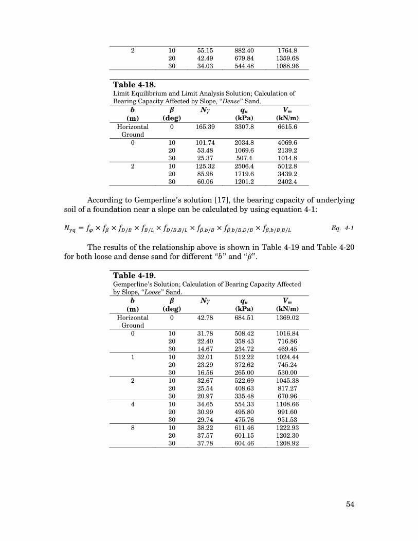
54

2

10 20 30

55.15 42.49 34.03

882.40 679.84 544.48

1764.8 1359.68 1088.96

Table 4-18. Limit Equilibrium and Limit Analysis Solution; Calculation of Bearing Capacity Affected by Slope, “Dense” Sand.

b (m)

β (deg)

Nγ qu (kPa)

Vm (kN/m)

Horizontal Ground

0 165.39 3307.8 6615.6

0

10 20 30

101.74 53.48 25.37

2034.8 1069.6 507.4

4069.6 2139.2 1014.8

2

10 20 30

125.32 85.98 60.06

2506.4 1719.6 1201.2

5012.8 3439.2 2402.4

According to Gemperline’s solution [17], the bearing capacity of underlying

soil of a foundation near a slope can be calculated by using equation 4-1: = × × / × / × / , / × , / × , / , / × , / , / Eq. 4-1

The results of the relationship above is shown in Table 4-19 and Table 4-20

for both loose and dense sand for different “b” and “β”.

Table 4-19. Gemperline’s Solution; Calculation of Bearing Capacity Affected by Slope, “Loose” Sand.

b (m)

β (deg)

Nγ qu (kPa)

Vm (kN/m)

Horizontal Ground

0 42.78 684.51 1369.02

0

10 20 30

31.78 22.40 14.67

508.42 358.43 234.72

1016.84 716.86 469.45

1

10 20 30

32.01 23.29 16.56

512.22 372.62 265.00

1024.44 745.24 530.00

2

10 20 30

32.67 25.54 20.97

522.69 408.63 335.48

1045.38 817.27 670.96

4

10 20 30

34.65 30.99 29.74

554.33 495.80 475.76

1108.66 991.60 951.53

8

10 20 30

38.22 37.57 37.78

611.46 601.15 604.46

1222.93 1202.30 1208.92

55

Table 4-20. Gemperline’s Solution; Calculation of Bearing Capacity Affected by Slope, “Dense” Sand.

b (m)

β (deg)

Nγ qu (kPa)

Vm (kN/m)

Horizontal Ground

0 162.47 2599.45 5198.89

0

10 20 30

120.67 85.07 55.71

1930.74 1361.14 891.37

3861.48 2722.28 1782.73

1

10 20 30

121.57 88.44 62.90

1945.16 1415.03 1006.34

3890.32 2830.05 2012.68

2

10 20 30

124.06 96.99 79.62

1984.92 1551.80 1273.99

3969.83 3103.59 2547.98

4

10 20 30

131.57 117.68 112.92

2105.08 1882.81 1806.72

4210.16 3765.62 3613.45

8 10 20 30

145.13 142.68 143.47

2322.04 2282.89 2295.45

4644.09 4565.77 4590.90

It is worthy to mention that in none of the solutions above, the effect of

dilation angle has been considered. Hence, the FLAC results for dense sand have a little difference with the theoretical solutions. 4.3 Calibrations

There are numerous effects due to alignment of the meshing, velocity and domain size in FLAC. In this part these parameters will be calibrated. But at the beginning, a general overview of soil behavior for different volume sizes are presented in Figure 4-2. The following figure provides different ultimate bearing capacities produced by the program for different widths (W, in meter) and different depths (D, in meter). It can be observed that by increasing the domain size, the final capacity reduces to a certain value. After that, only the failure displacement is changing.

56

Figure 4-2 - Different bearing capacities for various soil volume sizes, Loose Sand.

4.2.1 Meshing Alignment

At first, for a hypothesized domain of soil, the number and size of meshes are applied to be variant. Different sizes of meshing were tried and the following graph is produced:

Figure 4-3 - Meshing Alignment for loose sand

As it can be seen from Figure 4-3, it is obvious that the software is completely sensitive to number of cells and by increasing the number of cells, the bearing capacity decreases and reaches to theoretical value asymptotically. Due to the importance of the analysis time, the 4x4 meshing system is chosen that is very close to the theoretical value. 4x4 means that each 1 meter of the soil volume, is divided

0

500

1000

1500

2000

2500

0 0.1 0.2 0.3 0.4 0.5 0.6 0.7 0.8

V (k

N/m

)

Y Displacement (m)

(V-v)

TheoreticalW=4/D=3W=5/D=3W=6/D=3W=8/D=4W=10/D=6W=14/D=8W=18/D=10W=25/D=15W=30/D=18W=40/D=22

0

500

1000

1500

2000

2500

3000

0 0.2 0.4 0.6 0.8 1 1.2 1.4

V (k

N/m

)

Y Displacement (m)

(V-v)1x12x23x34x45x56x6Theoretical

57

to 4 elements in both vertical and horizontal direction that would be 25cm length in both directions. 4.2.2 Velocity Calibration

After finding the optimum case of meshing system, different values of velocity rate from -2×10-6 m/step to -200×10-6 m/step are applied to the foundation. Following graph shows the vertical bearing capacity vs. vertical displacement.

Figure 4-4 – Velocity Alignment, Loose sand.

As mentioned before, the time and speed of analysis is very important part of numerical modeling. However, this fact shouldn’t affect the accuracy of results. Considering this fact, and also as it can be observed from Figure 4-4, the velocity of -20×10-6 m/step is the highest one that approximately fitted to the theoretical value. Therefore, it is chosen as the base velocity of the project. 4.2.3 Width and Depth Calibration

In order to find the optimum size of the soil domain, different trial and error analysis have been performed. This calibration means to find the minimum depth and width of the soil domain in which the boundary effects are completely prevented. For this purpose, different widths from 5 to 40 meter and different depths from 5 to 30 meter by using the calibrated meshing size (4x4) and velocity rate (-20×10-6 m/step) are simulated. Therefore, according to the V-v diagram, the domain size is chosen. The results are presented in Figure 4-5 and Figure 4-6.

0

200

400

600

800

1000

1200

1400

1600

0 0.2 0.4 0.6 0.8 1 1.2 1.4 1.6

V (k

N/m

)

Y Displacement (m)

(V-v)

Y Velocity = -2E-6Y Velocity = -4E-6Y Velocity = -6E-6Y Velocity = -8E-6Y Velocity = -10E-6Y Velocity = -20E-6Y Velocity = -40E-6Y Velocity = -80E-6Y Velocity = -100E-6Y Velocity = -200E-6

58

Figure 4-5 - Width Alignment, loose sand.

As it can be seen from Figure 4-5, after 25 meter width the difference between initial stiffness is negligible. Hence, the 25 meter width is chosen as the final width of the domain.

Figure 4-6 - Depth Alignment, loose sand.

Also, it is illustrated from Figure 4-6 that after 15 meter depth the changes in initial stiffness can be neglected. Therefore, the 15 depth is chosen as the final depth of soil domain.

0

200

400

600

800

1000

1200

1400

1600

1800

0 0.1 0.2 0.3 0.4 0.5 0.6 0.7 0.8 0.9 1 1.1

V (k

N/m

)

Y Displacement (m)

(V-v)

W=5W=10W=15W=20W=25W=30W=35W=40Theoretical

0

200

400

600

800

1000

1200

1400

1600

0 0.1 0.2 0.3 0.4 0.5 0.6 0.7 0.8 0.9 1 1.1

V (k

N/m

)

Y Displacement (m)

(V-v)

D=5mD=10mD=15mD=20mD=25mD=30mTheoretical

59

4.3 Loose Sand By calibrating the meshing system, velocity rate and domain size, various

models have been simulated in order to find the interaction loci. In the beginning, the tests are performed to the foundation on horizontal ground overlying on described loose sand with vertical loading and also inclined loading (with inclination of α=+6°, +11°, +17° and +30°). Consequently, the simulations will be performed to sloped ground with different slope angles (β=10°, 20° and 30°) and also with different foundation distance to the slope edge (b=0, 1, 2, 4 and 8m). Direction of arrows in Figure 4-7 shows the positive side of all the graphs presented in this thesis.

Figure 4-7 - Direction of the positive side of graphs.

The results are presented in the following (Figure 4-8 to Figure 4-23): 4.3.1 Horizontal Ground

Figure 4-8 - Interaction Locus for Horizontal Ground, Loose Sand

-150

-100

-50

0

50

100

150

0 200 400 600 800 1000 1200 1400 1600H (k

N/m

)

V (kN/m)

V-H α = -30°α = -17°α = -11°α = -6°α = 0°α = 6°α = 11°α = 17°α = 30°

V

H

60

4.3.2 “b=0 m”

Figure 4-9 - Interaction Locus of 10° slope and b=0m, Loose Sand.

Figure 4-10 - Interaction Locus of 20° slope and b=0m, Loose Sand.

Figure 4-11 - Interaction Locus of 30° slope and b=0m, Loose Sand.

-150

-100

-50

0

50

100

150

0 200 400 600 800 1000 1200 1400 1600H(kN

/m)

V (kN/m)

V-H α = -30°α = -17°α = -11°α = -6°α = 0°α = 6°α = 11°α = 17°α = 30°

-150

-100

-50

0

50

100

150

0 200 400 600 800 1000 1200 1400 1600H (k

N/m

)

V (kN/m)

V-H α = -30°α = -17°α = -11°α = -6°α = 0°α = 6°α = 11°α = 17°α = 30°

-150

-100

-50

0

50

100

150

0 200 400 600 800 1000 1200 1400 1600H (k

N/m

)

V (kN/m)

V-H α = -30°α = -17°α = -11°α = -6°α = 0°α = 6°α = 11°α = 17°α = 30°

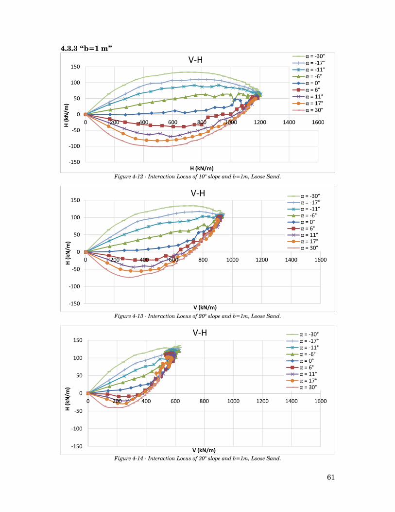
61

4.3.3 “b=1 m”

Figure 4-12 - Interaction Locus of 10° slope and b=1m, Loose Sand.

Figure 4-13 - Interaction Locus of 20° slope and b=1m, Loose Sand.

Figure 4-14 - Interaction Locus of 30° slope and b=1m, Loose Sand.

-150

-100

-50

0

50

100

150

0 200 400 600 800 1000 1200 1400 1600H (k

N/m

)

H (kN/m)

V-H α = -30°α = -17°α = -11°α = -6°α = 0°α = 6°α = 11°α = 17°α = 30°

-150

-100

-50

0

50

100

150

0 200 400 600 800 1000 1200 1400 1600H (k

N/m

)

V (kN/m)

V-H α = -30°α = -17°α = -11°α = -6°α = 0°α = 6°α = 11°α = 17°α = 30°

-150

-100

-50

0

50

100

150

0 200 400 600 800 1000 1200 1400 1600

H (k

N/m

)

V (kN/m)

V-H α = -30°α = -17°α = -11°α = -6°α = 0°α = 6°α = 11°α = 17°α = 30°

62

4.3.4 “b=2 m”

Figure 4-15 - Interaction Locus of 10° slope and b=2m, Loose Sand.

Figure 4-16 - Interaction Locus of 20° slope and b=2m, Loose Sand.

Figure 4-17 - Interaction Locus of 30° slope and b=2m, Loose Sand.

-150

-100

-50

0

50

100

150

0 200 400 600 800 1000 1200 1400 1600

H (k

N/m

)

V (kN/m)

V-H α = -30°α = -17°α = -11°α = -6°α = 0°α = 6°α = 11°α = 17°α = 30°

-150

-100

-50

0

50

100

150

0 200 400 600 800 1000 1200 1400 1600H (k

N/m

)

V (kN/m)

V-H α = -30°α = -17°α = -11°α = -6°α = 0°α = 6°α = 11°α = 17°α = 30°

-150

-100

-50

0

50

100

150

0 200 400 600 800 1000 1200 1400 1600H (k

N/m

)

V (kN/m)

V-H α = -30°α = -17°α = -11°α = -6°α = 0°α = 6°α = 11°α = 17°α = 30°

63

4.3.5 “b=4 m”

Figure 4-18 - Interaction Locus of 10° slope and b=4m, Loose Sand.

Figure 4-19 - Interaction Locus of 20° slope and b=4m, Loose Sand.

Figure 4-20 - Interaction Locus of 30° slope and b=4m, Loose Sand.

-150

-100

-50

0

50

100

150

0 200 400 600 800 1000 1200 1400 1600H (k

N/m

)

V (kN/m)

V-H α = -30°α = -17°α = -11°α = -6°α = 0°α = 6°α = 11°α = 17°α = 30°

-150

-100

-50

0

50

100

150

0 200 400 600 800 1000 1200 1400 1600

H (k

N/m

)

V (kN/m)

V-H α = -30°α = -17°α = -11°α = -6°α = 0°α = 6°α = 11°α = 17°α = 30°

-150

-100

-50

0

50

100

150

0 200 400 600 800 1000 1200 1400 1600H (k

N/m

)

V (kN/m)

V-H α = -30°α = -17°α = -11°α = -6°α = 0°α = 6°α = 11°α = 17°α = 30°

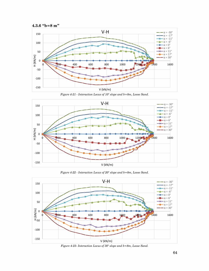
64

4.3.6 “b=8 m”

Figure 4-21 - Interaction Locus of 10° slope and b=8m, Loose Sand.

Figure 4-22 - Interaction Locus of 20° slope and b=8m, Loose Sand.

Figure 4-23- Interaction Locus of 30° slope and b=8m, Loose Sand.

-150

-100

-50

0

50

100

150

0 200 400 600 800 1000 1200 1400 1600H (k

N/m

)

V (kN/m)

V-H α = -30°α = -17°α = -11°α = -6°α = 0°α = 6°α = 11°α = 17°α = 30°

-150

-100

-50

0

50

100

150

0 200 400 600 800 1000 1200 1400 1600H (k

N/m

)

V (kN/m)

V-H α = -30°α = -17°α = -11°α = -6°α = 0°α = 6°α = 11°α = 17°α = 30°

-150

-100

-50

0

50

100

150

0 200 400 600 800 1000 1200 1400 1600

H (k

N/m

)

V (kN/m)

V-H α = -30°α = -17°α = -11°α = -6°α = 0°α = 6°α = 11°α = 17°α = 30°

65

4.3.7 Comparison of Performed Tests In the following (Figure 4-24 to Figure 4-32) all the results and charts are

compared together with two different aspects: (a) different slope angles and same distance of foundation to slope edge, (b) different distance of foundation to slope edge with same slope angles.

4.3.7.1 Different Values of b

Figure 4-24 - Comparison of Interaction Locus for b=0m with Different Angles, "Loose" Sand

Figure 4-25 - Comparison of Interaction Locus for “b=1m” with Different Angles, "Loose" Sand

-150

-100

-50

0

50

100

150

0 200 400 600 800 1000 1200 1400 1600H (k

N/m

)

V (kN/m)

V-HHorizontal Ground10 deg20 deg30 deg

-150

-100

-50

0

50

100

150

0 200 400 600 800 1000 1200 1400 1600H (k

N/m

)

V (kN/m)

V-HHorizontal Ground10 deg20 deg30 deg

66

Figure 4-26 - Comparison of Interaction Locus for “b=2m” with Different Angles, "Loose" Sand

Figure 4-27 - Comparison of Interaction Locus for “b=4m” with Different Angles, "Loose" Sand

Figure 4-28 - Comparison of Interaction Locus for “b=8m” with Different Angles, "Loose" Sand

-150

-100

-50

0

50

100

150

0 200 400 600 800 1000 1200 1400 1600H (k

N/m

)

V (kN/m)

V-HHorizontal Ground10 deg20 deg30 deg

-150

-100

-50

0

50

100

150

0 200 400 600 800 1000 1200 1400 1600

H (k

N/m

)

V (kN/m)

V-HHorizontal Ground10 deg20 deg30 deg

-150

-100

-50

0

50

100

150

0 200 400 600 800 1000 1200 1400 1600H (k

N/m

)

V (kN/m)

V-HHorizontal Ground10 deg20 deg30 deg

67

4.3.7.2 Different Values of Slope Angle (β)

Figure 4-29- Comparison of Interaction Locus for “β=10°” with Different b, "Loose" Sand

Figure 4-30- Comparison of Interaction Locus for “β=20°” with Different b, "Loose" Sand

Figure 4-31- Comparison of Interaction Locus for “β=30°” with Different b, "Loose" Sand

-150

-100

-50

0

50

100

150

0 200 400 600 800 1000 1200 1400 1600H (k

N/m

)

V (kN/m)

V-HHorizontal Groundb=8b=4b=2b=1b=0

-150

-100

-50

0

50

100

150

0 200 400 600 800 1000 1200 1400 1600H (k

N/m

)

V (kN/m)

V-HHorizontal Groundb=8b=4b=2b=1b=0

-150

-100

-50

0

50

100

150

0 200 400 600 800 1000 1200 1400 1600H (k

N/m

)

V (kN/m)

V-HHorizontal Groundb=8b=4b=2b=1b=0

68

Figure 4-32 - Comparison of different b and β vs. Vm

As it can be seen in the Figure 4-32, the vertical bearing capacity decreases by increasing the slope inclination and decreasing the distance of foundation to the slope edge. Also the interaction locus loses its area due to the effect of slope and distance “b”. As far as the slope is steeper and the edge of slope is closer to the foundation, the interaction domain decreases.

0

200

400

600

800

1000

1200

1400

1600

0 1 2 3 4 5 6 7 8 9

V (k

N/m

)

b (m)

Different "b" and "β", Loose Sand

10 deg20 deg30 degHorizontal Ground

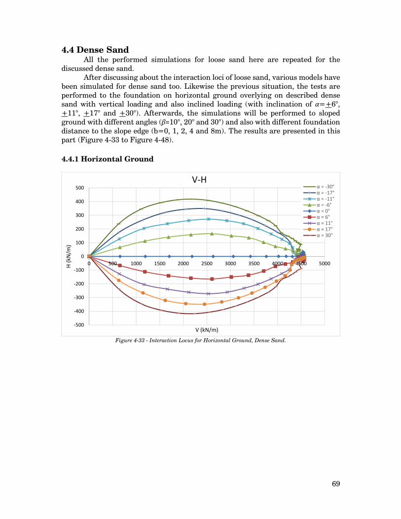
69

4.4 Dense Sand All the performed simulations for loose sand here are repeated for the

discussed dense sand. After discussing about the interaction loci of loose sand, various models have

been simulated for dense sand too. Likewise the previous situation, the tests are performed to the foundation on horizontal ground overlying on described dense sand with vertical loading and also inclined loading (with inclination of α=+6°, +11°, +17° and +30°). Afterwards, the simulations will be performed to sloped ground with different angles (β=10°, 20° and 30°) and also with different foundation distance to the slope edge (b=0, 1, 2, 4 and 8m). The results are presented in this part (Figure 4-33 to Figure 4-48). 4.4.1 Horizontal Ground

Figure 4-33 - Interaction Locus for Horizontal Ground, Dense Sand.

-500

-400

-300

-200

-100

0

100

200

300

400

500

0 500 1000 1500 2000 2500 3000 3500 4000 4500 5000H (k

N/m

)

V (kN/m)

V-Hα = -30°α = -17°α = -11°α = -6°α = 0°α = 6°α = 11°α = 17°α = 30°

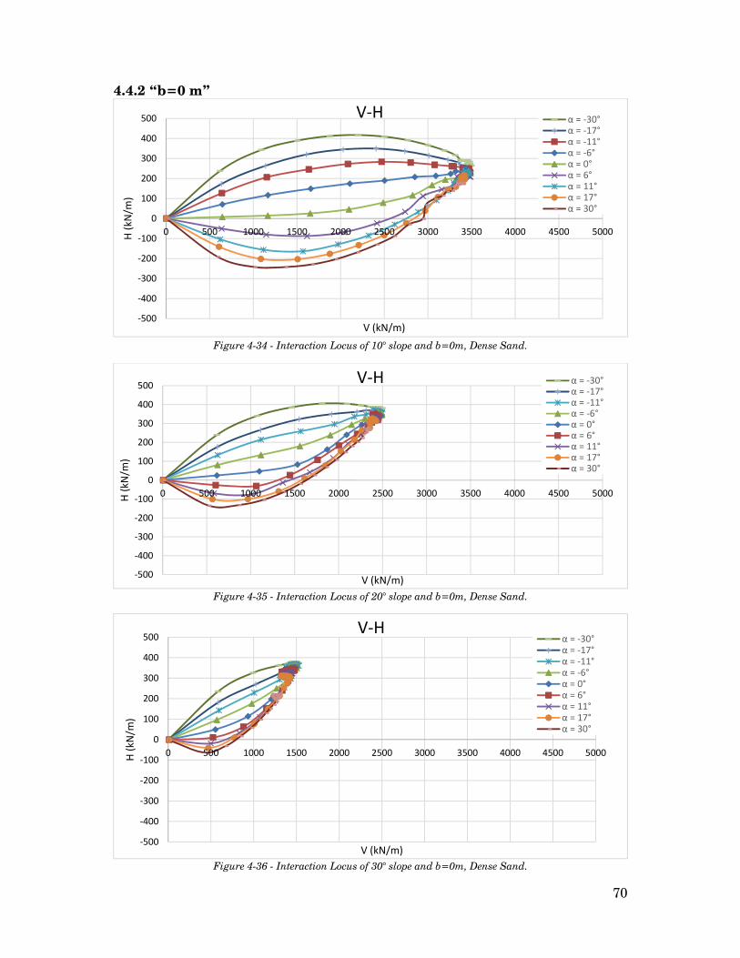
70

4.4.2 “b=0 m”

Figure 4-34 - Interaction Locus of 10° slope and b=0m, Dense Sand.

Figure 4-35 - Interaction Locus of 20° slope and b=0m, Dense Sand.

Figure 4-36 - Interaction Locus of 30° slope and b=0m, Dense Sand.

-500

-400

-300

-200

-100

0

100

200

300

400

500

0 500 1000 1500 2000 2500 3000 3500 4000 4500 5000H (k

N/m

)

V (kN/m)

V-H α = -30°α = -17°α = -11°α = -6°α = 0°α = 6°α = 11°α = 17°α = 30°

-500

-400

-300

-200

-100

0

100

200

300

400

500

0 500 1000 1500 2000 2500 3000 3500 4000 4500 5000H (k

N/m

)

V (kN/m)

V-H α = -30°α = -17°α = -11°α = -6°α = 0°α = 6°α = 11°α = 17°α = 30°

-500

-400

-300

-200

-100

0

100

200

300

400

500

0 500 1000 1500 2000 2500 3000 3500 4000 4500 5000H (k

N/m

)

V (kN/m)

V-Hα = -30°α = -17°α = -11°α = -6°α = 0°α = 6°α = 11°α = 17°α = 30°

71

4.4.3 “b=1 m”

Figure 4-37 - Interaction Locus of 10° slope and b=1m, Dense Sand.

Figure 4-38 - Interaction Locus of 20° slope and b=1m, Dense Sand.

Figure 4-39 - Interaction Locus of 30° slope and b=1m, Dense Sand.

-500

-400

-300

-200

-100

0

100

200

300

400

500

0 500 1000 1500 2000 2500 3000 3500 4000 4500 5000H (k

N/m

)

V (kN/m)

V-H α = -30°α = -17°α = -11°α = -6°α = 0°α = 6°α = 11°α = 17°α = 30°

-500

-400

-300

-200

-100

0

100

200

300

400

500

0 500 1000 1500 2000 2500 3000 3500 4000 4500 5000H (k

N/m

)

V (kN/m)

V-H α = -30°α = -17°α = -11°α = -6°α = 0°α = 6°α = 11°α = 17°α = 30°

-500

-400

-300

-200

-100

0

100

200

300

400

500

0 500 1000 1500 2000 2500 3000 3500 4000 4500 5000H (k

N/m

)

V (kN/m)

V-Hα = -30°α = -17°α = -11°α = -6°α = 0°α = 6°α = 11°α = 17°α = 30°

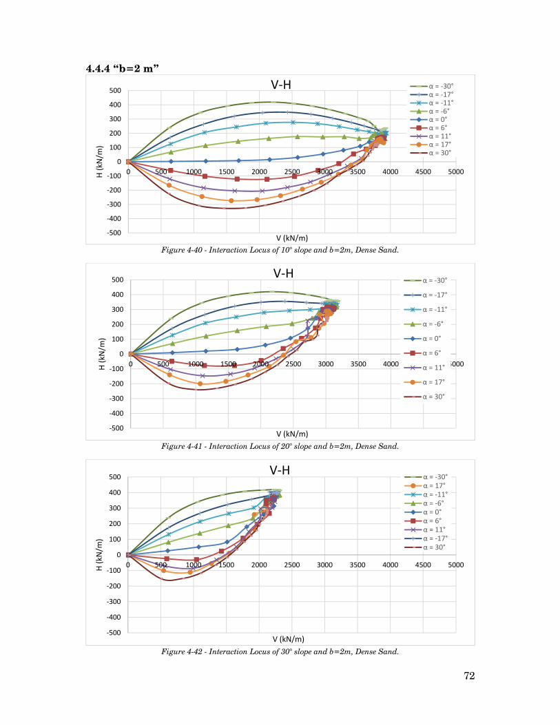
72

4.4.4 “b=2 m”

Figure 4-40 - Interaction Locus of 10° slope and b=2m, Dense Sand.

Figure 4-41 - Interaction Locus of 20° slope and b=2m, Dense Sand.

Figure 4-42 - Interaction Locus of 30° slope and b=2m, Dense Sand.

-500

-400

-300

-200

-100

0

100

200

300

400

500

0 500 1000 1500 2000 2500 3000 3500 4000 4500 5000H (k

N/m

)

V (kN/m)

V-H α = -30°α = -17°α = -11°α = -6°α = 0°α = 6°α = 11°α = 17°α = 30°

-500

-400

-300

-200

-100

0

100

200

300

400

500

0 500 1000 1500 2000 2500 3000 3500 4000 4500 5000H (k

N/m

)

V (kN/m)

V-Hα = -30°

α = -17°

α = -11°

α = -6°

α = 0°

α = 6°

α = 11°

α = 17°

α = 30°

-500

-400

-300

-200

-100

0

100

200

300

400

500

0 500 1000 1500 2000 2500 3000 3500 4000 4500 5000H (k

N/m

)

V (kN/m)

V-H α = -30°α = 17°α = -11°α = -6°α = 0°α = 6°α = 11°α = -17°α = 30°

73

4.4.5 “b=4 m”

Figure 4-43 - Interaction Locus of 10° slope and b=4m, Dense Sand.

Figure 4-44 - Interaction Locus of 20° slope and b=4m, Dense Sand.

Figure 4-45 - Interaction Locus of 30° slope and b=4m, Dense Sand.

-500

-400

-300

-200

-100

0

100

200

300

400

500

0 500 1000 1500 2000 2500 3000 3500 4000 4500 5000H (k

N/m

)

V (kN/m)

V-H α = -30°α = -17°α = -11°α = -6°α = 0°α = 6°α = 11°α = 17°α = 30°

-500

-400

-300

-200

-100

0

100

200

300

400

500

0 500 1000 1500 2000 2500 3000 3500 4000 4500 5000H (k

N/m

)

V (kN/m)

V-H α = -30°α = -17°α = -11°α = -6°α = 0°α = 6°α = 11°α = 17°α = 30°

-500

-400

-300

-200

-100

0

100

200

300

400

500

0 500 1000 1500 2000 2500 3000 3500 4000 4500 5000H (k

N/m

)

V (kN/m)

V-H α = -30°α = -17°α = -11°α = -6°α = 0°α = 6°α = 11°α = 17°α = 30°

74

4.4.6 “b=8 m”

Figure 4-46 - Interaction Locus of 10° slope and b=8m, Dense Sand.

Figure 4-47 - Interaction Locus of 20° slope and b=8m, Dense Sand.

Figure 4-48 - Interaction Locus of 30° slope and b=8m, Dense Sand.

-500

-400

-300

-200

-100

0

100

200

300

400

500

0 500 1000 1500 2000 2500 3000 3500 4000 4500 5000H (k

N/m

)

V (kN/m)

V-H α = -30°α = -17°α = -11°α = -6°α = 0°α = 6°α = 11°α = 17°α = 30°

-500

-400

-300

-200

-100

0

100

200

300

400

500

0 500 1000 1500 2000 2500 3000 3500 4000 4500 5000H (k

N/m

)

V (kN/m)

V-H α = -30°α = -17°α = -11°α = -6°α = 0°α = 6°α = 11°α = 17°α = 30°

-500

-400

-300

-200

-100

0

100

200

300

400

500

0 500 1000 1500 2000 2500 3000 3500 4000 4500 5000H (k

N/m

)

V (kN/m)

V-H α = -30°α = -17°α = -11°α = -6°α = 0°α = 6°α = 11°α = 17°α = 30°

75

4.4.7 Comparison of Performed Tests

Similar to the comparison performed in loose sand case, all the results and charts are compared together with two different aspects: (a) different slope angles and same distance of foundation to slope edge, (b) different distance of foundation to slope edge and same slope angles. These comparisons are shown in Figure 4-49 to Figure 4-57).

4.4.7.1 Different Values of b

Figure 4-49 - Comparison of Interaction Locus for “b=0m” with Different Angles, "Dense" Sand

Figure 4-50 - Comparison of Interaction Locus for “b=1m” with Different Angles, "Dense" Sand

-500

-400

-300

-200

-100

0

100

200

300

400

500

0 500 1000 1500 2000 2500 3000 3500 4000 4500 5000H (k

N/m

)

V (kN/m)

V-H Horizontal Ground10 deg20 deg30 deg

-500

-400

-300

-200

-100

0

100

200

300

400

500

0 1000 2000 3000 4000 5000H (k

N/m

)

V (kN/m)

V-HHorizontal Ground10 deg20 deg30 deg

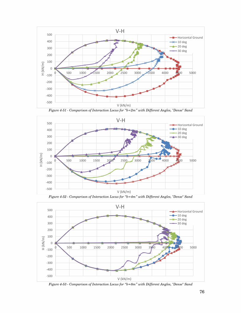
76

Figure 4-51 - Comparison of Interaction Locus for “b=2m” with Different Angles, "Dense" Sand

Figure 4-52 - Comparison of Interaction Locus for “b=4m” with Different Angles, "Dense" Sand

Figure 4-53 - Comparison of Interaction Locus for “b=8m” with Different Angles, "Dense" Sand

-500

-400

-300

-200

-100

0

100

200

300

400

500

0 500 1000 1500 2000 2500 3000 3500 4000 4500 5000H (k

N/m

)

V (kN/m)

V-HHorizontal Ground10 deg20 deg30 deg

-500

-400

-300

-200

-100

0

100

200

300

400

500

0 500 1000 1500 2000 2500 3000 3500 4000 4500 5000

H (k

N/m

)

V (kN/m)

V-HHorizontal Ground10 deg20 deg30 deg

-500

-400

-300

-200

-100

0

100

200

300

400

500

0 500 1000 1500 2000 2500 3000 3500 4000 4500 5000H (k

N/m

)

V (kN/m)

V-HHorizontal Ground10 deg20 deg30 deg

77

4.4.7.2 Different Values of Slope Angle (β)

Figure 4-54 - Comparison of Interaction Locus for “β=10°” with Different b, "Dense" Sand

Figure 4-55 - Comparison of Interaction Locus for “β=20°” with Different b, "Dense" Sand

Figure 4-56 - Comparison of Interaction Locus for “β=30°” with Different b, "Dense" Sand

-500

-400

-300

-200

-100

0

100

200

300

400

500

0 500 1000 1500 2000 2500 3000 3500 4000 4500 5000H (k

N/m

)

V (kN/m)

V-H Horizontal Groundb=8b=4b=2b=1b=0

-500

-400

-300

-200

-100

0

100

200

300

400

500

0 500 1000 1500 2000 2500 3000 3500 4000 4500 5000H (k

N/m

)

V (kN/m)

V-H Horizontal Groundb=8b=4b=2b=1b=0

-500

-400

-300

-200

-100

0

100

200

300

400

500

0 500 1000 1500 2000 2500 3000 3500 4000 4500 5000H (k

N/m

)

V (kN/m)

V-H Horizontal Groundb=8b=4b=2b=1b=0

78

Figure 4-57 - Comparison of different b and β vs. Vm

As it can be seen in the Figure 4-57, the behavior of the dense sand behavior is similar to loose sand. The vertical bearing capacity decreases by increasing the slope inclination and decreasing the distance of foundation to the slope edge. Also the interaction locus loses its area due to the effect of slope and distance “b”. As far as the slope is steeper and the edge of slope is closer to the foundation, the interaction domain decreases. It also should be mentioned that unlike the loose sand that the bearing capacities for different situations reached together almost in 8 meter distance, in dense sand they will reach at farther distance.

Figure 4-58 presents a comparison of interaction locus of loose sand and

dense sand. The graph shows clearly the effect of the friction angle and dilation angle on the bearing capacity and interaction domain of the soil.

Figure 4-58 - Comparison of Interaction Locus for “Loose” Sand and “Dense” Sand

0

500

1000

1500

2000

2500

3000

3500

4000

4500

5000

0 1 2 3 4 5 6 7 8 9

V (k

N/m

)

b (m)

Different "b" and "β", Dense Sand

10 deg20 deg30 degHorizontal Ground

-500

-400

-300

-200

-100

0

100

200

300

400

500

0 500 1000 1500 2000 2500 3000 3500 4000 4500 5000

H (k

N/m

)

V (kN/m)

V-HDense SandLoose Sand

79

4.5 Validations with Theoretical Solutions In this section the obtained results will be validated with theoretical

solutions. As discussed before in chapter 2 (part 2.2.2 and 2.2.3), some solutions have presented by different authors for inclination factors. For controlling the results which obtained from FLAC, the methods provided by Meyerhof, Hansen and Vesic are utilized. By using the load inclination angle, corresponding horizontal loads to vertical bearing capacity can be found, and afterwards, by employing these loads the interaction domain can be drawn. The following figures (Figure 4-59 and Figure 4-60) present comparisons of different results proposed by mentioned authors:

Figure 4-59 - Different Bearing Capacities on Horizontal Ground Proposed by Different Authors,

“Loose” Sand

Figure 4-60 - Different Bearing Capacities on Horizontal Ground Proposed by Different Authors,

“Dense” Sand

0

40

80

120

160

0 200 400 600 800 1000 1200 1400 1600

H (k

N/m

)

V (kN/m)

V-HVesicHansenMeyerhof

0

50

100

150

200

250

300

350

400

450

500

0 500 1000 1500 2000 2500 3000 3500 4000 4500

H (k

N/m

)

V (kN/m)

V-HVesicHansenMeyerhof

80

Figure 4-61 and Figure 4-62 provide comparisons between the theoretical results and numerical results for horizontal ground for loose sand dense sand.

Figure 4-61 - Comparison of Numerical Results with Theoretical Values, "Loose" Sand.

Figure 4-62 - Comparison of Numerical Results with Theoretical Values, "Dense" Sand.

It can be illustrated that for loose sand the results obtained from program approximately are fitted to theoretical results. Nevertheless, due to the effect of dilation angle, there is a difference between FLAC results and theoretical solutions for dense sand. The comparisons are developed for the sloped ground and are presented in Figure 4-63 to Figure 4-92.

-160

-120

-80

-40

0

40

80

120

160

0 200 400 600 800 1000 1200 1400 1600H (k

N/m

)

V (kN/m)

V-HVesic

Hansen

-500

-400

-300

-200

-100

0

100

200

300

400

500

0 500 1000 1500 2000 2500 3000 3500 4000 4500 5000

H (k

N/m

)

V (kN/m)

V-HVesicHansenMeyerhofNumerical Results

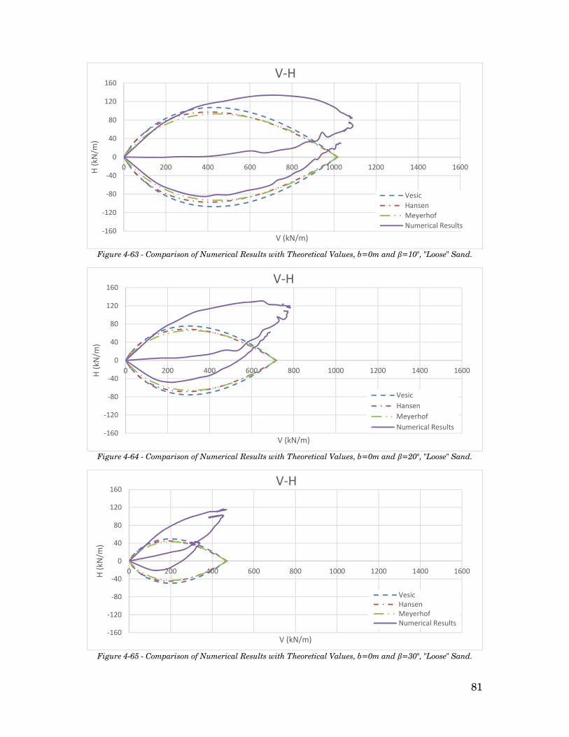
81

Figure 4-63 - Comparison of Numerical Results with Theoretical Values, b=0m and β=10°, "Loose" Sand.

Figure 4-64 - Comparison of Numerical Results with Theoretical Values, b=0m and β=20°, "Loose" Sand.

Figure 4-65 - Comparison of Numerical Results with Theoretical Values, b=0m and β=30°, "Loose" Sand.

-160

-120

-80

-40

0

40

80

120

160

0 200 400 600 800 1000 1200 1400 1600H (k

N/m

)

V (kN/m)

V-H

VesicHansenMeyerhofNumerical Results

-160

-120

-80

-40

0

40

80

120

160

0 200 400 600 800 1000 1200 1400 1600H (k

N/m

)

V (kN/m)

V-H

VesicHansenMeyerhofNumerical Results

-160

-120

-80

-40

0

40

80

120

160

0 200 400 600 800 1000 1200 1400 1600H (k

N/m

)

V (kN/m)

V-H

VesicHansenMeyerhofNumerical Results

82

Figure 4-66 - Comparison of Numerical Results with Theoretical Values, b=1m and β=10°, "Loose" Sand.

Figure 4-67 - Comparison of Numerical Results with Theoretical Values, b=1m and β=20°, "Loose" Sand.

Figure 4-68 - Comparison of Numerical Results with Theoretical Values, b=1m and β=30°, "Loose" Sand.

-160

-120

-80

-40

0

40

80

120

160

0 200 400 600 800 1000 1200 1400 1600H (k

N/m

)

V (kN/m)

V-H

VesicHansenMeyerhofNumerical Results

-160

-120

-80

-40

0

40

80

120

160

0 200 400 600 800 1000 1200 1400 1600H (k

N/m

)

V (kN/m)

V-H

VesicHansenMeyerhofNumerical Results

-160

-120

-80

-40

0

40

80

120

160

0 200 400 600 800 1000 1200 1400 1600H (k

N/m

)

V (kN/m)

V-H

VesicHansenMeyerhofNumerical Results

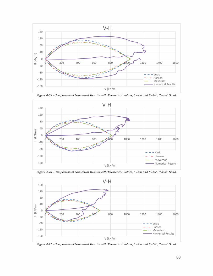
83

Figure 4-69 - Comparison of Numerical Results with Theoretical Values, b=2m and β=10°, "Loose" Sand.

Figure 4-70 - Comparison of Numerical Results with Theoretical Values, b=2m and β=20°, "Loose" Sand.

Figure 4-71 - Comparison of Numerical Results with Theoretical Values, b=2m and β=30°, "Loose" Sand.

-160

-120

-80

-40

0

40

80

120

160

0 200 400 600 800 1000 1200 1400 1600H (k

N/m

)

V (kN/m)

V-H

VesicHansenMeyerhofNumerical Results

-160

-120

-80

-40

0

40

80

120

160

0 200 400 600 800 1000 1200 1400 1600H (k

N/m

)

V (kN/m)

V-H

VesicHansenMeyerhofNumerical Results

-160

-120

-80

-40

0

40

80

120

160

0 200 400 600 800 1000 1200 1400 1600H (k

N/m

)

V (kN/m)

V-H

VesicHansenMeyerhofNumerical Results

84

Figure 4-72 - Comparison of Numerical Results with Theoretical Values, b=4m and β=10°, "Loose" Sand.

Figure 4-73 - Comparison of Numerical Results with Theoretical Values, b=4m and β=20°, "Loose" Sand.

Figure 4-74 - Comparison of Numerical Results with Theoretical Values, b=4m and β=30°, "Loose" Sand.

-160

-120

-80

-40

0

40

80

120

160

0 200 400 600 800 1000 1200 1400 1600H (k

N/m

)

V (kN/m)

V-H

VesicHansenMeyerhofNumerical Results

-160

-120

-80

-40

0

40

80

120

160

0 200 400 600 800 1000 1200 1400 1600H (k

N/m

)

V (kN/m)

V-H

VesicHansenMeyerhofNumerical Results

-160

-120

-80

-40

0

40

80

120

160

0 200 400 600 800 1000 1200 1400 1600H (k

N/m

)

V (kN/m)

V-H

VesicHansenMeyerhofNumerical Results

85

Figure 4-75 - Comparison of Numerical Results with Theoretical Values, b=8m and β=10°, "Loose" Sand.

Figure 4-76 - Comparison of Numerical Results with Theoretical Values, b=8m and β=20°, "Loose" Sand.

Figure 4-77 - Comparison of Numerical Results with Theoretical Values, b=8m and β=30°, "Loose" Sand.

-160

-120

-80

-40

0

40

80

120

160

0 200 400 600 800 1000 1200 1400 1600H (k

N/m

)

V (kN/m)

V-H

VesicHansenMeyerhofNumerical Results

-160

-120

-80

-40

0

40

80

120

160

0 200 400 600 800 1000 1200 1400 1600H (k

N/m

)

V (kN/m)

V-H

VesicHansenMeyerhofNumerical Results

-160

-120

-80

-40

0

40

80

120

160

0 200 400 600 800 1000 1200 1400 1600H (k

N/m

)

V (kN/m)

V-H

VesicHansenMeyerhofNumerical Results

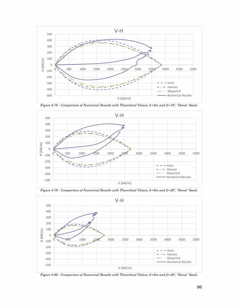
86

Figure 4-78 - Comparison of Numerical Results with Theoretical Values, b=0m and β=10°, "Dense" Sand.

Figure 4-79 - Comparison of Numerical Results with Theoretical Values, b=0m and β=20°, "Dense" Sand.

Figure 4-80 - Comparison of Numerical Results with Theoretical Values, b=0m and β=30°, "Dense" Sand.

-500

-400

-300

-200

-100

0

100

200

300

400

500

0 500 1000 1500 2000 2500 3000 3500 4000 4500 5000H (k

N/m

)

V (kN/m)

V-H

VesicHansenMeyerhofNumerical Results

-500

-400

-300

-200

-100

0

100

200

300

400

500

0 500 1000 1500 2000 2500 3000 3500 4000 4500 5000H (k

N/m

)

V (kN/m)

V-H

VesicHansenMeyerhofNumerical Results

-500

-400

-300

-200

-100

0

100

200

300

400

500

0 500 1000 1500 2000 2500 3000 3500 4000 4500 5000H (k

N/m

)

V (kN/m)

V-H

VesicHansenMeyerhofNumerical Results

87

Figure 4-81 - Comparison of Numerical Results with Theoretical Values, b=1m and β=10°, "Dense" Sand.

Figure 4-82 - Comparison of Numerical Results with Theoretical Values, b=1m and β=20°, "Dense" Sand.

Figure 4-83 - Comparison of Numerical Results with Theoretical Values, b=1m and β=30°, "Dense" Sand.

-500

-400

-300

-200

-100

0

100

200

300

400

500

0 500 1000 1500 2000 2500 3000 3500 4000 4500 5000H (k

N/m

)

V (kN/m)

V-H

VesicHansenMeyerhofNumerical Results

-500

-400

-300

-200

-100

0

100

200

300

400

500

0 500 1000 1500 2000 2500 3000 3500 4000 4500 5000H (k

N/m

)

V (kN/m)

V-H

VesicHansenMeyerhofNumerical Results

-500

-400

-300

-200

-100

0

100

200

300

400

500

0 500 1000 1500 2000 2500 3000 3500 4000 4500 5000H (k

N/m

)

V (kN/m)

V-H

VesicHansenMeyerhofNumerical Results

88

Figure 4-84 - Comparison of Numerical Results with Theoretical Values, b=2m and β=10°, "Dense" Sand.

Figure 4-85 - Comparison of Numerical Results with Theoretical Values, b=2m and β=20°, "Dense" Sand.

Figure 4-86 - Comparison of Numerical Results with Theoretical Values, b=2m and β=30°, "Dense" Sand.

-500

-400

-300

-200

-100

0

100

200

300

400

500

0 500 1000 1500 2000 2500 3000 3500 4000 4500 5000H (k

N/m

)

V (kN/m)

V-H

VesicHansenMeyerhofNumerical Results

-500

-400

-300

-200

-100

0

100

200

300

400

500

0 500 1000 1500 2000 2500 3000 3500 4000 4500 5000H (k

N/m

)

V (kN/m)

V-H

VesicHansenMeyerhofNumerical Results

-500

-400

-300

-200

-100

0

100

200

300

400

500

0 500 1000 1500 2000 2500 3000 3500 4000 4500 5000H (k

N/m

)

V (kN/m)

V-H

VesicHansenMeyerhofNumerical Results

89

Figure 4-87 - Comparison of Numerical Results with Theoretical Values, b=4m and β=10°, "Dense" Sand.

Figure 4-88 - Comparison of Numerical Results with Theoretical Values, b=4m and β=20°, "Dense" Sand.

Figure 4-89 - Comparison of Numerical Results with Theoretical Values, b=4m and β=30°, "Dense" Sand.

-500

-400

-300

-200

-100

0

100

200

300

400

500

0 500 1000 1500 2000 2500 3000 3500 4000 4500 5000H (k

N/m

)

V (kN/m)

V-H

VesicHansenMeyerhofNumerical Results

-500

-400

-300

-200

-100

0

100

200

300

400

500

0 500 1000 1500 2000 2500 3000 3500 4000 4500 5000H (k

N/m

)

V (kN/m)

V-H

VesicHansenMeyerhofNumerical Results

-500

-400

-300

-200

-100

0

100

200

300

400

500

0 500 1000 1500 2000 2500 3000 3500 4000 4500 5000H (k

N/m

)

V (kN/m)

V-H

VesicHansenMeyerhofNumerical Results

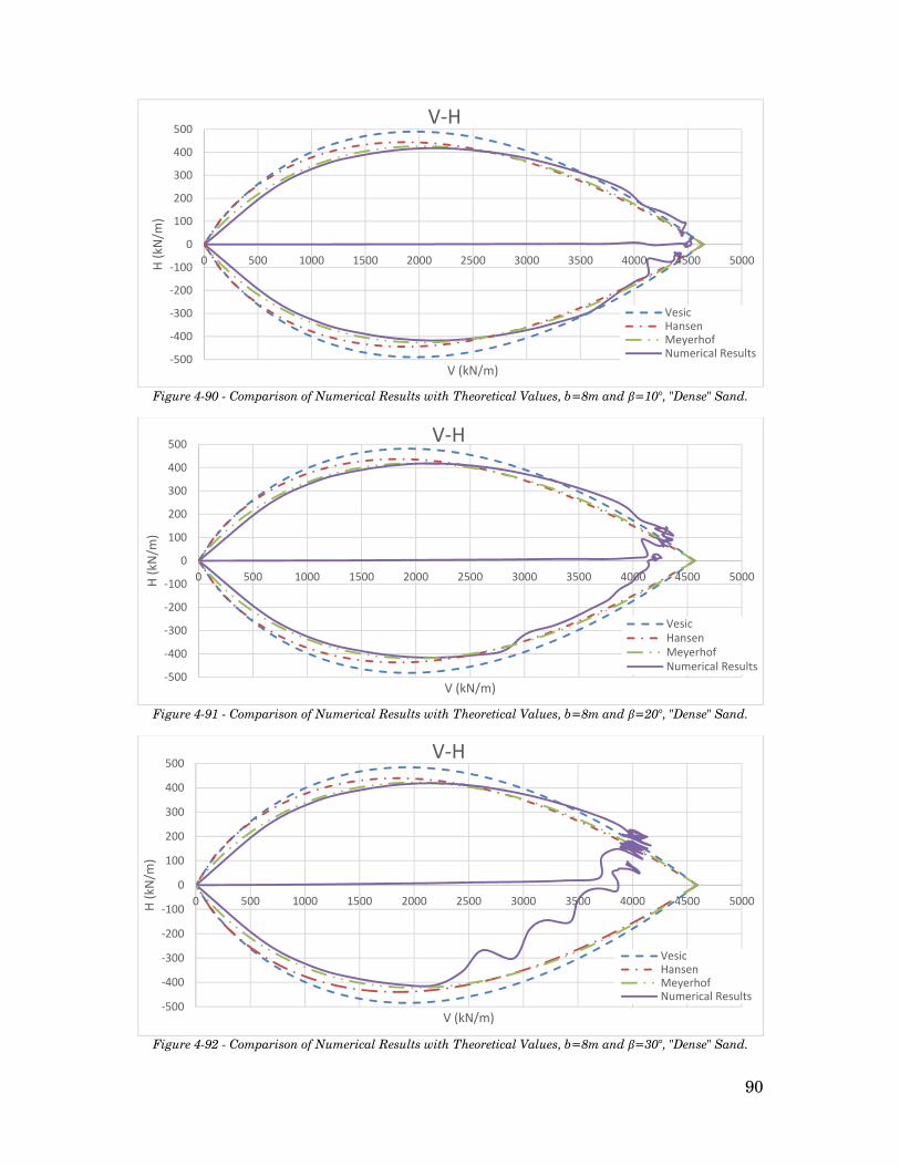
90

Figure 4-90 - Comparison of Numerical Results with Theoretical Values, b=8m and β=10°, "Dense" Sand.

Figure 4-91 - Comparison of Numerical Results with Theoretical Values, b=8m and β=20°, "Dense" Sand.

Figure 4-92 - Comparison of Numerical Results with Theoretical Values, b=8m and β=30°, "Dense" Sand.

-500

-400

-300

-200

-100

0

100

200

300

400

500

0 500 1000 1500 2000 2500 3000 3500 4000 4500 5000H (k

N/m

)

V (kN/m)

V-H

VesicHansenMeyerhofNumerical Results

-500

-400

-300

-200

-100

0

100

200

300

400

500

0 500 1000 1500 2000 2500 3000 3500 4000 4500 5000H (k

N/m

)

V (kN/m)

V-H

VesicHansenMeyerhofNumerical Results

-500

-400

-300

-200

-100

0

100

200

300

400

500

0 500 1000 1500 2000 2500 3000 3500 4000 4500 5000H (k

N/m

)

V (kN/m)

V-H

VesicHansenMeyerhofNumerical Results

91

Numerical results are also compared to the Nova’s solution for horizontal ground for both loose sand and dense sand: ( , , ) ≡ − 1 − = 0 β=0.95 Eq. 4-2

Where, Vmax is the central vertical load capacity of the foundation. Figure 4-93 and Figure 4-94 present the comparison of interaction domain produced from FLAC for different load inclinations and interaction domain obtained from Nova’s equation.

Figure 4-93 - Comparison of Numerical Interaction Locus with Nova Solution, Loose Sand.

Figure 4-94 - Comparison of Numerical Interaction Locus with Nova Solution, Dense Sand.

-200

-150

-100

-50

0

50

100

150

200

0 200 400 600 800 1000 1200 1400 1600

H (k

N/m

)

V (kN/m)

V-Hα = -30°α = -17°α = -11°α = -6°α = 0°α = 6°α = 11°α = 17°α = 30°Nova

-600

-400

-200

0

200

400

600

0 500 1000 1500 2000 2500 3000 3500 4000 4500 5000H (k

N/m

)

V (kN/m)

V-H α = -30°α = -17°α = -11°α = -6°α = 0°α = 6°α = 11°α = 17°α = 30°Nova

92

4.6 Developing an Analytical Solution

According to the performed simulations, using the interactions loci produced by the program and considering Nova’s equation as the basis equation, numerous trial and errors analysis have been done in order to find the best analytical solution of the interaction locus. In the proposed equation in this dissertation, different variables that affect the interaction domain have been considered (b, β, α, φ and ψ). The proposed solution is presented in equation 4-3: ∗ = ( ) 1 − . × × × × Eq. 4-3

Where: = ( ). ( )

= 2.2sin(1.5 ) = (1 − 1.2 ) = cos + 1 −

ψ = dilation angle (°) φ = friction angle (°) β = slope angle (°) b = distance of foundation to the slope edge (m) B = width of foundation (m) α = load inclination to the vertical (°)

The best fitted analytical interaction domain is obtained by rotating the value of “H*” using the rotation matrix (equation 4-4), with the angle of rotation “θ” which is presented in equation 4.5. This angle is developed after many trial and errors analysis and it is dependent to the slope angle “β” and ratio of “b/B”: = sin( ) + cos( ) ∗ Eq. 4-4 = . Eq. 4-5

Subsequently, by employing the proposed solution, the analytical interaction

loci are drawn and along with, a comparison is made between the numerical and analytical solution (Figure 4-95 to Figure 4-124).

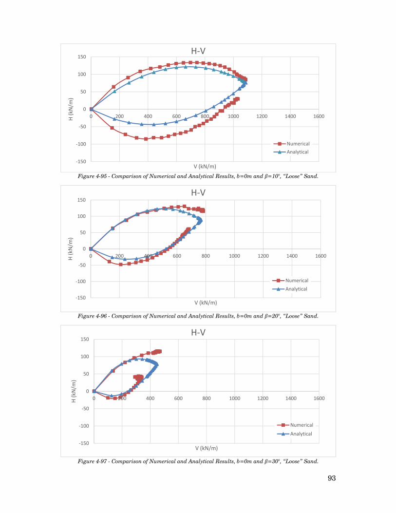
93

Figure 4-95 - Comparison of Numerical and Analytical Results, b=0m and β=10°, “Loose” Sand.

Figure 4-96 - Comparison of Numerical and Analytical Results, b=0m and β=20°, “Loose” Sand.

Figure 4-97 - Comparison of Numerical and Analytical Results, b=0m and β=30°, “Loose” Sand.

-150

-100

-50

0

50

100

150

0 200 400 600 800 1000 1200 1400 1600H (k

N/m

)

V (kN/m)

H-V

NumericalAnalytical

-150

-100

-50

0

50

100

150

0 200 400 600 800 1000 1200 1400 1600H (k

N/m

)

V (kN/m)

H-V

NumericalAnalytical

-150

-100

-50

0

50

100

150

0 200 400 600 800 1000 1200 1400 1600H (k

N/m

)

V (kN/m)

H-V

Numerical

Analytical

94

Figure 4-98 - Comparison of Numerical and Analytical Results, b=1m and β=10°, “Loose” Sand.

Figure 4-99 - Comparison of Numerical and Analytical Results, b=1m and β=20°, “Loose” Sand.

Figure 4-100 - Comparison of Numerical and Analytical Results, b=1m and β=30°, “Loose” Sand.

-150

-100

-50

0

50

100

150

0 200 400 600 800 1000 1200 1400 1600H (k

N/m

)

V (kN/m)

H-V

Numerical

Analytical

-150

-100

-50

0

50

100

150

0 200 400 600 800 1000 1200 1400 1600H (k

N/m

)

V (kN/m)

H-V

Numerical

Analytical

-150

-100

-50

0

50

100

150

0 200 400 600 800 1000 1200 1400 1600H (k

N/m

)

V (kN/m)

H-V

Numerical

Analytical

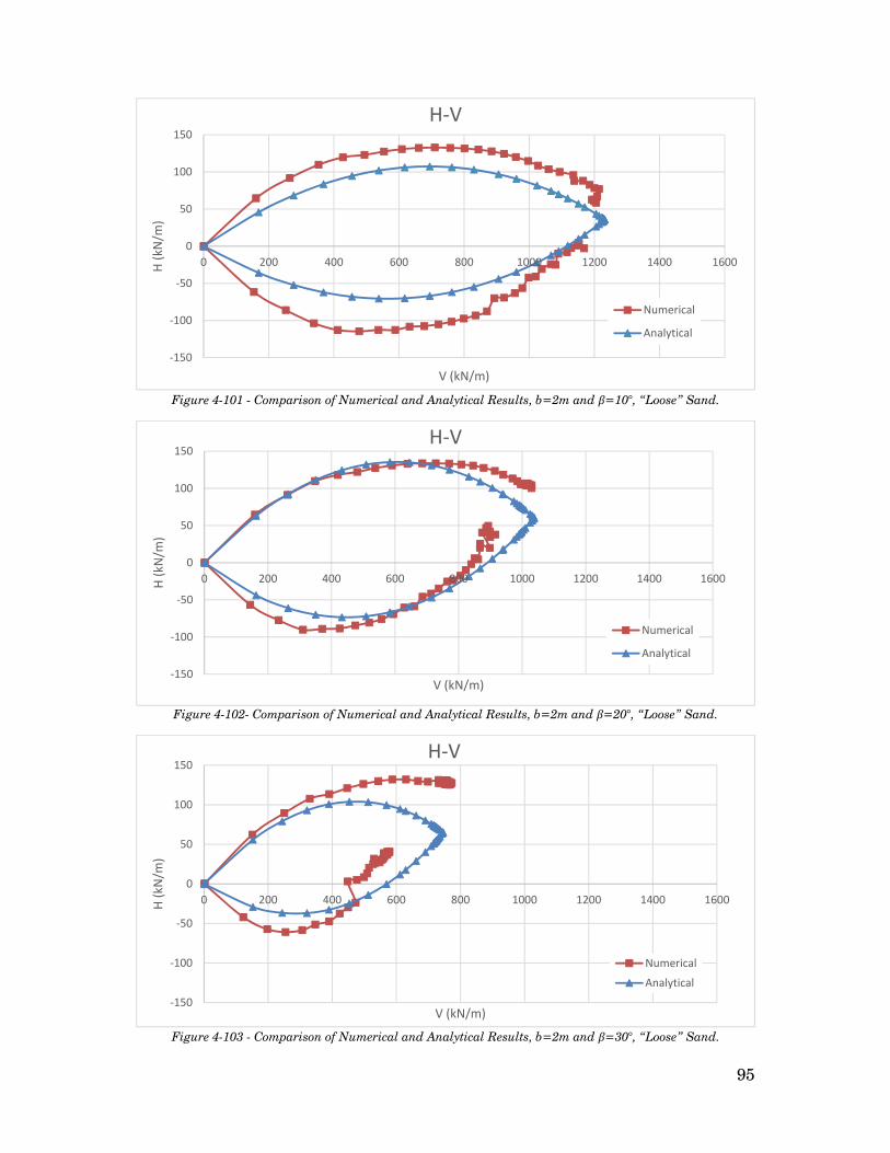
95

Figure 4-101 - Comparison of Numerical and Analytical Results, b=2m and β=10°, “Loose” Sand.

Figure 4-102- Comparison of Numerical and Analytical Results, b=2m and β=20°, “Loose” Sand.

Figure 4-103 - Comparison of Numerical and Analytical Results, b=2m and β=30°, “Loose” Sand.

-150

-100

-50

0

50

100

150

0 200 400 600 800 1000 1200 1400 1600H (k

N/m

)

V (kN/m)

H-V

Numerical

Analytical

-150

-100

-50

0

50

100

150

0 200 400 600 800 1000 1200 1400 1600H (k

N/m

)

V (kN/m)

H-V

Numerical

Analytical

-150

-100

-50

0

50

100

150

0 200 400 600 800 1000 1200 1400 1600H (k

N/m

)

V (kN/m)

H-V

Numerical

Analytical

96

Figure 4-104 - Comparison of Numerical and Analytical Results, b=4m and β=10°, “Loose” Sand.

Figure 4-105 - Comparison of Numerical and Analytical Results, b=4m and β=20°, “Loose” Sand.

Figure 4-106 - Comparison of Numerical and Analytical Results, b=4m and β=30°, “Loose” Sand.

-150

-100

-50

0

50

100

150

0 200 400 600 800 1000 1200 1400 1600H (k

N/m

)

V (kN/m)

H-V

Numerical

Analytical

-150

-100

-50

0

50

100

150

0 200 400 600 800 1000 1200 1400 1600H (k

N/m

)

V (kN/m)

H-V

NumericalAnalytical

-150

-100

-50

0

50

100

150

0 200 400 600 800 1000 1200 1400 1600H (k

N/m

)

V (kN/m)

H-V

NumericalAnalytical

97

Figure 4-107 - Comparison of Numerical and Analytical Results, b=8m and β=10°, “Loose” Sand.

Figure 4-108 - Comparison of Numerical and Analytical Results, b=8m and β=20°, “Loose” Sand.

Figure 4-109 - Comparison of Numerical and Analytical Results, b=8m and β=30°, “Loose” Sand.

-150

-100

-50

0

50

100

150

0 200 400 600 800 1000 1200 1400 1600H (k

N/m

)

V (kN/m)

H-V

NumericalAnalytical

-150

-100

-50

0

50

100

150

0 200 400 600 800 1000 1200 1400 1600H (k

N/m

)

V (kN/m)

H-V

NumericalAnalytical

-150

-100

-50

0

50

100

150

0 200 400 600 800 1000 1200 1400 1600H (k

N/m

)

V (kN/m)

H-V

NumericalAnalytical

98

Figure 4-110 - Comparison of Numerical and Analytical Results, b=0m and β=10°, “Dense” Sand.

Figure 4-111 - Comparison of Numerical and Analytical Results, b=0m and β=20°, “Dense” Sand.

Figure 4-112 - Comparison of Numerical and Analytical Results, b=0m and β=30°, “Dense” Sand.

-500

-400

-300

-200

-100

0

100

200

300

400

500

0 500 1000 1500 2000 2500 3000 3500 4000 4500 5000H (k

N/m

)

V (kN/m)

H-V

NumericalAnalytical

-500

-400

-300

-200

-100

0

100

200

300

400

500

0 500 1000 1500 2000 2500 3000 3500 4000 4500 5000H (k

N/m

)

V (kN/m)

H-V

NumericalAnalytical

-500

-400

-300

-200

-100

0

100

200

300

400

500

0 500 1000 1500 2000 2500 3000 3500 4000 4500 5000H (k

N/m

)

V (kN/m)

H-V

NumericalAnalytical

99

Figure 4-113 - Comparison of Numerical and Analytical Results, b=1m and β=10°, “Dense” Sand.

Figure 4-114 - Comparison of Numerical and Analytical Results, b=1m and β=20°, “Dense” Sand.

Figure 4-115 - Comparison of Numerical and Analytical Results, b=1m and β=30°, “Dense” Sand.

-500

-400

-300

-200

-100

0

100

200

300

400

500

0 500 1000 1500 2000 2500 3000 3500 4000 4500 5000H (k

N/m

)

V (kN/m)

H-V

NumericalAnalytical

-500

-400

-300

-200

-100

0

100

200

300

400

500

0 500 1000 1500 2000 2500 3000 3500 4000 4500 5000H (k

N/m

)

V (kN/m)

H-V

NumericalAnalytical

-500

-400

-300

-200

-100

0

100

200

300

400

500

0 500 1000 1500 2000 2500 3000 3500 4000 4500 5000H (k

N/m

)

V (kN/m)

H-V

NumericalAnalytical

100

Figure 4-116 - Comparison of Numerical and Analytical Results, b=2m and β=10°, “Dense” Sand.

Figure 4-117 - Comparison of Numerical and Analytical Results, b=2m and β=20°, “Dense” Sand.

Figure 4-118 - Comparison of Numerical and Analytical Results, b=2m and β=30°, “Dense” Sand.

-500

-400

-300

-200

-100

0

100

200

300

400

500

0 500 1000 1500 2000 2500 3000 3500 4000 4500 5000H (k

N/m

)

V (kN/m)

H-V

NumericalAnalytical

-500

-400

-300

-200

-100

0

100

200

300

400

500

0 500 1000 1500 2000 2500 3000 3500 4000 4500 5000H (k

N/m

)

V (kN/m)

H-V

NumericalAnalytical

-500

-400

-300

-200

-100

0

100

200

300

400

500

0 500 1000 1500 2000 2500 3000 3500 4000 4500 5000H (k

N/m

)

V (kN/m)

H-V

NumericalAnalytical

101

Figure 4-119 - Comparison of Numerical and Analytical Results, b=4m and β=10°, “Dense” Sand.

Figure 4-120 - Comparison of Numerical and Analytical Results, b=4m and β=20°, “Dense” Sand.

Figure 4-121 - Comparison of Numerical and Analytical Results, b=4m and β=30°, “Dense” Sand.

-500

-400

-300

-200

-100

0

100

200

300

400

500

0 500 1000 1500 2000 2500 3000 3500 4000 4500 5000H (k

N/m

)

V (kN/m)

H-V

NumericalAnalytical

-500

-400

-300

-200

-100

0

100

200

300

400

500

0 500 1000 1500 2000 2500 3000 3500 4000 4500 5000H (k

N/m

)

V (kN/m)

H-V

NumericalAnalytical

-500

-400

-300

-200

-100

0

100

200

300

400

500

0 500 1000 1500 2000 2500 3000 3500 4000 4500 5000H (k

N/m

)

V (kN/m)

H-V

NumericalAnalytical

102

Figure 4-122 - Comparison of Numerical and Analytical Results, b=8m and β=10°, “Dense” Sand.

Figure 4-123 - Comparison of Numerical and Analytical Results, b=8m and β=20°, “Dense” Sand.

Figure 4-124 - Comparison of Numerical and Analytical Results, b=8m and β=30°, “Dense” Sand.

-600-500-400-300-200-100

0100200300400500600

0 500 1000 1500 2000 2500 3000 3500 4000 4500 5000H (k

N/m

)

V (kN/m)

H-V

NumericalAnalytical

-500

-400

-300

-200

-100

0

100

200

300

400

500

0 500 1000 1500 2000 2500 3000 3500 4000 4500 5000H (k

N/m

)

V (kN/m)

H-V

NumericalAnalytical

-500

-400

-300

-200

-100

0

100

200

300

400

500

0 500 1000 1500 2000 2500 3000 3500 4000 4500 5000H (k

N/m

)

V (kN/m)

H-V

NumericalAnalytical

103

4.7 Proposing a Design Chart In this part, by using the results produced by FLAC, a numerical design chart

for granular soils is proposed. For assessing this design chart, 48 extra simulations have been done by considering the effect of dilation angle. The dilation angles of (0° and 5°) and (0°, 10° and 15°) were taken into account for loose sand and dense sand respectively. According to this fact, different ultimate loads are shown in Figure 4-125 and Figure 4-126.

Figure 4-125 - Comparison of different "b" and "β" for different dilation angles, Loose Sand.

Figure 4-126 - Comparison of different "b" and "β" for different dilation angles, Dense Sand.

As it can be observed from figures above, increasing the dilation angle increases the ultimate bearing capacity.

0

200

400

600

800

1000

1200

1400

1600

0 1 2 3 4 5 6 7 8 9

V (k

N/m

)

b (m)

Different "b" and "β", Loose Sand

10 deg20 deg30 degHorizontal Ground

Dilation = 0Dilation = 10

0

1000

2000

3000

4000

5000

6000

0 1 2 3 4 5 6 7 8 9

V (k

N/m

)

b (m)

Differetn "b" and "β", Dense Sand

10 deg20 deg30 degHorizontal Ground

Dilation = 0°Dilation = 10°Dilation = 15°

104

By using the numerical results and performing some trial and errors analysis, an analytical solution is proposed in order to take into account the effect of dilation angle in the bearing capacity. Along with, a design chart is developed to assess the bearing capacity factor, Nγ. Afterwards, by calculating the effect of dilation angle using equation (eq. 4-7) and taking the value of Nγ using Figure 4-127, the bearing capacity qu can be estimated (eq. 4-6).

= 0.5 Eq. 4-6

Where, = (1 + 1.3 sin( )) Eq. 4-7

Figure 4-127 presents the bearing capacity factors (Nγ) for different slope

inclinations and foundation distances to slope edge.

Figure 4-127 - Proposed design chart for finding the ultimate bearing capacity of foundation on top of a slope.

0

10

20

30

40

50

60

70

80

90

100

110

120

0 1 2 3 4 5 6 7 8 9

Nγ

Foundation distance to slope edge, b (m)

Design Chart

φ=40°

φ=35°

β=0°β=10° β=20° β=30°β=0°β=10°β=20°β=30°

105

5. Conclusion

This project has illustrated the use of explicit finite difference software (FLAC) to analyze the behavior exhibited by a slope due to a foundation loading. This chapter presents the overall findings of the project. The problem of a rigid foundation resting near a slope or cut is commonly experienced in engineering practice. Some of the major examples of this problem include mobile phone towers, bridge abutments and basement construction of high–rise buildings. This problem has been the major focus of this research project, which has looked into creating a comprehensive set of design charts for the footing on slope problem for clayey soils.

Elasto-Plastic analysis for analyzing the bearing capacity of a shallow foundation built near a slope was presented in this project paper. This analysis has been done by applying the explicit finite differencing method built within FLAC. Initially numerical results were compared with other available solutions. This comparison was done in order to verify the quality of the results obtained from this software program. After validation of these models had been completed satisfactorily, extensive parametric studies were conducted into the effect of the b/B, slope angle (β), as well as the loading inclination angle (α), friction angle (φ) and dilation angle (ψ).

1) The reduction of bearing capacity due to loading inclination was experienced.

2) It was seen that increasing the friction angle and dilation angle have a direct relation with the increasing of the bearing capacity.

3) Another finding was that increasing the steepness of the slope can have

significant effects on ultimate bearing capacity. The general trend shown was that for increasing slope angle the bearing capacity was reduced.

4) The positioning of a footing also has considerable effect on ultimate bearing capacity. Significant gains in ultimate bearing capacity can be achieved by moving a foundation small distances from the edge of a slope. This is due to the changes that occur in the failure mechanism by moving further from a slope edge. Increased soil heaving and less defined slip lines are both changes that occur due to moving further from a slope. Moving a foundation even half its width away from a slope may bring considerable bearing capacity gains.

5) It was also observed that the inclination of the ground causes asymmetry in the interaction locus. By increasing the slope angle, the more asymmetry induces.

106

After completing the parametric studies, a new solution has been proposed to determine the interaction locus of vertical and horizontal loading of a foundation on top of a slope. Along with, new design charts and solution considering the dilation angle of soil for calculating the ultimate bearing capacity of shallow foundations has been developed. These demonstrated the variation in bearing capacity due to footing distance ratio, slope angle, load inclination, friction angle and dilation angle. The base of the proposed solution for determining the interaction locus was the equation suggested by Nova in 1988. The proposed solution is validated and compatible with all the numerical results.

107

References 1. Audibert, J.M.E., & Nyman, K.J., (1977), Soil Restraint against Horizontal Motion of

Pipes, Journal of Geotechnical Engineering Division, ASCE, vol. 103, No GT10, pp 1119-1142.

2. Bartlett, S. F., 2010. Mohr-Coulomb Model. 3. Butterfield, R. & Gottardi, G., 1994. A complete three—dimensional failure envelope

for shallow footings on sand. 4. Calvetti, F., Di Prisco, C. & Nova, R., 2004. Experimental and numerical analysis of

soil-pipe interaction.

5. Caquot, A., & J. Kerisel. 1949. Tables for the calculation of passive pressure, active pressure, and bearing capacity of foundations. Paris: Gauthier-Villars.

6. Casagrande, A., & N. Carrillo. 1954. Shear failure in anisotropic materials, in

Contribution to soil mechanics 1941–53, Boston Society of Civil Engineers, 122. 7. Castelli, F. & Motta, E., 2006. Bearing Capacity of Strip Footings near Slopes. 8. Chao, J., 2000. Shallow Foundations, Bridge Engineering Handbook.

9. Chen, W. F., 1975. Limit analysis and soil plasticity. Elsevier Scientific Publishing

Company. 10. Cocchetti, G., Di Prisco, C., Galli, A. & Nova, R., 2009. Soil–pipeline interaction along

unstable slopes: a coupled three-dimensional approach. 11. Coduto, Donald (2001), Foundation Design, Prentice-Hall.

12. Das, B. M., 2006. Principles of Foundation Engineering, 7th edition.

13. Das, B. M., 2009. Bearing Capacity and Settlement of Shallow Foundations.

14. DeBeer, E. E. 1975. Analysis of shallow foundations, in Geotechnical modeling and

applications, ed. S. M. Sayed, 212. Gulf Publishing Co. Houston, USA.

15. Di Prisco, C. & Galli, A., 2006. Soil-pipe interaction under monotonic and cyclic loads: experimental and numerical modelling.

16. Di Prisco, C., Nova, R. & Corengia, A., 2004. A model for landslide-pipe interaction

analysis. Soils and Foundations.

17. Gemperline, M.C., 1988. Centrifugal Modeling of Shallow Foundations. Soil Properties Evaluation from Centrifugal Models and Field Performance.

18. Georgiadis, K., 2009. The influence of load inclination on the undrained bearing

capacity of strip footings on slopes

108

19. Georgiadis, M. & Butterfield, R., 1988. Displacements of footings on sand under

eccentric and inclined loads.

20. Gottardi, G. & Butterfield, R., 1993. Bearing capacity of surface footing on sand under general planar load.

21. Graham, J. & Stuart, J., 1971. Scale and boundary effects in foundation analysis.

22. Graham, J., Andrews, M. & Shields, D.H., 1988. Stress Characteristics for Shallow

Footings in Cohesionless Slopes, Canadian Geotechnical Journal, v. 25, p. 238—249.

23. Hansen, JB., 1970. A revised and extended formula for bearing capacity.

24. Itasca, Consulting Group Inc. (2001a). FLAC: Fast Lagrangian Analysis of Continua User’s Guide.

25. Keskin, M. et al., 2012. Model Studies of Bearing Capacity of Strip Footing on Sand

Slope.

26. Kimmerling, R. E., 2002. Geotechnical engineering circular no. 6, Shallow Foundations.

27. Kusakabe, O., Kimura, T. & Yamaguchi, H., 1981. Bearing Capacity of Slopes Under

Strip Loads on the Top Surfaces, Soils and Foundations, Japanese Society of Soil Mechanics and Foundation Engineering, v. 21, n. 4, p. 29—40.

28. Lundgren, H., & K. Mortensen. 1953. Determination by the theory of plasticity of the

bearing capacity of continuous footings on sand, in Proc., III Int. Conf. Soil Mech. Found. Eng., Zurich, Switzerland, 1: 409.

29. Lyle, N. R., 2009. Comprehensive Design Charts for the footing on Slope Problem.

30. Martin, C. M. 2005. Exact bearing capacity calculations using the method of

characteristics. Proc., 11thInt. Conf. IACMAG, Turin, 4: 441

31. McCarthy, D.F., 2007. Essentials of Soil Mechanics and Foundations, 7th edition, Pearson, New Jersey.

32. Merifield, R. S., A. V. Lyamin, S. W. Sloan, & H. S. Yu. 2003. Three-dimensional lower

bound solutions for stability of plate anchors in clay. J. Geotech. Geoenv. Eng., ASCE, 129(3): 243.

33. Meyerhof, G. G. & Hanna, A. M., 1978. Ultimate bearing capacity of foundations on

layered soils under inclined load.

34. Meyerhof, G. G. 1963. Some recent research on the bearing capacity of foundations. Canadian Geotech. J. 1(1): 16

35. Meyerhof, G.G., 1951. The Ultimate Bearing Capacity of Foundations.

36. Meyerhof, G.G., 1957. Ultimate Bearing Capacity of Foundations on Slopes.

109

37. Michalowski, R. L., 1997. An estimate of the influence of soil weight on bearing

capacity using limit analysis. Soils and Foundations. 37(4): 57

38. Narita, K. & Yamaguchi, H., 1990. Bearing Capacity Analysis of Foundations on Slopes by use of Log--Spiral Sliding Surfaces, Soils and Foundations, Japanese Society of Soil Mechanics and Foundation Engineering, v. 30, n. 3, p. 144—152.

39. Nova, R. & Montrasio, L., 1991. Settlements of shallow foundations on sand.

40. Prandtl, L., 1921. Uber die eindringungsfestigkeit plastisher baustoffe und die

festigkeit von schneiden. Z. Ang. Math. Mech. 1(1): 15.

41. Saran, S., Sud, V.K. & Handa, S.C., 1989. Bearing Capacity of Footings Adjacent to Slopes, Journal of Geotechnical Engineering, v. 115, no. 4, p. 553—573.

42. Shiau, J. & Smith, C., 2006. Numerical Analysis of Passive Earth Pressures with Interfaces

43. Shields, D., Chandler, N. & Garnier, J., 1990. ‘Bearing Capacity of Foundations in

Slopes’, Journal of Geotechnical Engineering, v. 116, n. 3, p. 528—537.

44. Shields, D.H., Scott, J.D., Bauer, G.E., Deschemes, J.H. & Barsvary, A.K., 1977. Bearing Capacity of Foundations near Slopes. Proceeding of the 9th International Conference on Soil Mechanics and Foundation Engineering, v. 1, p. 715—720.

45. Smith, C.A. & Shiau, J.S., 2007. Bearing Capacity of Footings near Slopes, Common

Ground, Proceedings of the 10th Australian and New Zealand Conference on Geomechanics, Brisbane Australia.

46. Tatsuoka, F., Huang, C. C., Morimoto, T. & Okahara, M., 1989. Stress Characteristics

for Shallow Footing in Cohesionless Slopes: Discussion

47. Terzaghi, K., 1943. Theoretical Soil Mechanics.

48. Ticof, J., (1977). Surface footings on sand under general planar loads. PhD Thesis, University of Southampton, UK.

49. Vesic, A.S., 1973. Analysis of ultimate load of shallow foundations. Journal of the Soil

Mechanics and Foundations Division.

50. Watson, J. F., 2008. Investigation of the Bearing Capacity of Shallow Footings Located near Slopes

51. Yamaguchi, H. & Kunitomo, N., 1992. Three—Dimensional Bearing Capacity Analysis

of Foundations by use of a Method of Slices, Soils and Foundations, Japanese Society of Soil Mechanics and Foundation Engineering, v. 32, n. 4, p. 143—155.

52. Zhang, J., Stewart, D. P., & Randolph, J. H.(2002). “Modeling of shallowly embedded

offshore pipelines in calcareous sand.” J. Geo-tech. Geoenviron. Eng., 128(5), 363–371.

110

POLITECNICO DI MILANO

Department of Civil, Environmental and Land Management Engineering Master of Science in Civil Engineering

INTERACTION DOMAIN OF SHALLOW FOUNDATIONS ON THE TOP OF A SLOPE

A Master thesis submitted to Department of Civil, Environmental and Land Management Engineering in partial fulfillment of the requirements for the degree of Master of Science in Civil Engineering for Risk Mitigation. Submitted by: Supervised by: _________________________ _________________________ Mehdi Nouri Prof. Andrea Galli Student ID: 770776 Department of Civil, Environmental

and Land Management Engineering, Politecnico di Milano

Piazza L. da Vinci, 32, I-20133, Milan