INTENSIVE AGRICULTURE AND POLITICAL ECONOMY OF THE YAGUACHI CHIEFDOM OF GUAYAS BASIN, COASTAL ECUADOR.

by

Florencio Delgado-Espinoza

BA University of Texas at San Antonio, 1993

Submitted to the Graduate Faculty of

Arts and Sciences in partial fulfillment

of the requirements for the degree of

Doctor of Philosophy

University of Pittsburgh

2002

ii

UNIVERSITY OF PITTSBURGH

FACULTY OF ARTS AND SCIENCES

This dissertation was presented

by

Florencio Delgado-Espinoza

It was defended on

September 14, 2001

and approved by

Marc Bermman

Olivier DeMontmollin

Billie DeWalt

Robert D. Drennan Dissertation Director

iii

Copyright by Florencio Delgado-Espinoza 2002

iv

Intensive Agriculture and Political Economy in the Yaguachi Chiefdom of the lower Guayas

Basin, Coastal Ecuador.

Florencio Delgado-Espinoza, PhD

University of Pittsburgh, 2002

This dissertation examines the relationship between intensive agriculture and the

development of chiefly societies in the Lower Guayas Basin, coastal Ecuador. The Yaguachi

chiefdom arose in the area at least during the Integration Period AD 700-Spanish contact. This

social formation built intensive agriculture technology (raised fields) and large earth mounds.

Two approaches, top-down and a bottom-up, are contrasted to identify where along a socio-

political continuum the organization of the Yaguachi chiefdom lay. The research aimed to

reconstruct regional settlement patterns using the spatial distribution of sites and their

relationships to raised field zones. Data gathering included methods such as aerial photogrametry

and subsurface testing. Excavation was conducted through shovel tests, auger probes and a

limited number of excavation units. The surveyed area consisted of 428. 29 km², and survey

results identified 622 mounds clustered into 16 settlements located along the borders of a large

zone of raised fields. These settlements form a three-tiered hierarchy with three main regional

centers, sub-centers, agricultural villages and isolated households. Raised fields were found in

large tracts. Sites show a strong tendency to cluster, and, for the most part, large centers had

large supporting populations. Those centers are located adjacent to raised field zones. Evidence

at the core of one of the sites indicates that considerable feasting activities took place.

Differences in access to resources among households correspond to their location within the

three-tiered hierarchy. Raised field construction required large labor inputs, and they provided

v

large outputs. Mound building activities, feasting and burial practices indicate strong sense of

community in the local population. This evidence leads to the conclusions that local chiefs were

engaged in the management of raised field production, and that public mound building and

feasting activities served to make this possible.

vi

FOREWORD

This written work is the conclusion of a process of graduate studies that I started few

years ago when I wandered to the US as a foreign student. Along this road many people helped

me in the transition from a rural Third World setting to US college life. The list is large and

acknowledging all would constitute a completely new written report in itself. I will try to name

the most important with the apologies to those that I am surely forgetting. In San Antonio, the

members of the faculty at the University of Texas at San Antonio and staff of the Center for

Archaeological research provided support during my first years in the US, especially R.E.W.

Adams, Rene Muñoz, Gerry Raymond and Robert Hard helped me to gain a better understanding

of American archaeology.

The faculty of the department of anthropology of the University of Pittsburgh has been

most helpful in shaping my knowledge of anthropology. I wish to thank the members of my

doctoral committee, Marc Berman, Olivier de Montmollin, Billie DeWalt and Robert Drennan,

for the input and suggestions that made this work more understandable. Robert Drennan has

provided support and has guided me through the entire process. This work would not have been

written without his help. Dick has shown interest and involvement in this project since its

inception, and he always made time for the painful task of reading various drafts and helping me

to make this paper readable. He gave me lots of support and has been always there whenever I

needed help. His dedication and commitment to his students and Latin American archaeology is

something I will always admire.

The Center for Latin American Studies has also been supportive and funded previous

fieldwork through its summer field grant. My studies at Pittsburgh were possible thanks to the

vii

Howard Heinz Fellowship for Latin American Archaeology. Funding for Field Research came

from National Science Foundation Dissertation Improvement Grant # 9724998.

I would not have been able to get to this stage without the help of Kimberlee Marshall,

Louis Prouet, James Young and Deborah Young. Many thanks also go out to Karen Stothert and

her family. In Ecuador, the Instituto Nacional de Patrimonio Cultural granted me permission to

conduct fieldwork, thanks to José Chancay who has been supportive of this research. Pedro

Silva at the Universidad de Milagro provided accommodations for the material. The Arreaga

family in Vuelta Larga provided invaluable help. Doña Rosa Saltos granted permission to work

at the site Jerusalén. Thanks also go out to the local finqueros who allowed us to wander on their

land strangely looking for sherds. Special mention deserves Peter Stahl who analyzed animal

bones from this project.

The personnel of the Proyecto Arqueológico Yaguachi (PAY) worked interminable

hours, frequently donating their time to the Project. Freddy Acuña, Hugo Gómez, Danilo

Delgado, Giovanni Delgado, Alejandro Delgado, Julio Espinoza, Verónica Arreaga, Carmen

Arreaga, Manuel Terán, Carlos González, Yolanda Merino, Robert Sweet and Josefina Vásquez

formed a group that made field experience very enjoyable. In Quito, I have received help from

Jose Vásquez, Cecilia Pazmiño, and Nicolás Vásquez

In Pittsburgh, my friends and colleagues made my experience a blast. Thanks to María

Auxiliadora Cordero, Claudia Rivera, Sonia Alconini, Vincent McElhinny, Ana María Boada,

John Vandenbosh, Alejandro Chu, Viviana Siveroni, Andrea Cuéllar and Rich Scaglion, who

have all been supportive. Thanks also to my friends Freddy Quinche, Fernando and Patricio

Morán. I always gained so much knowledge through discussions about Ecuadorian politics,

viii

economics and other issues with Armando Muyulema and Patrick Wilson. They have also been

supportive friends. Debbie Truhan gave me important comments and help editing early drafts.

This work would have not been possible without the dedication of Josefina Vásquez, field

and lab supervisor. Sharing field and laboratory experiences with her has been one of the best

rewards I have had in my life.

Deseo agradecer a mi familia, mi padre Cesar Delgado, con la esperanza de que algún

día pueda leer estas notas. Gracias a mis hermanos, quienes en forma desinteresada y

comedida me ayudaron en todo momento. Agradezco a mi madre quien me inculcó la

perseverancia; Madre gracias.

ix

TABLE OF CONTENTS

Chapter 1 __________________________________________________________________ 1 Chiefdoms and Intensive Agriculture _____________________________________________ 1 Chapter 2 _________________________________________________________________ 11 The Organization of Intensive Agriculture ________________________________________ 11

The Top-Down Approach to Intensive Agricultural Production ______________________ 11 The Bottom-Up Approach to the Organization of Intensification Technology ___________ 18

Settlement Patterning and Raised Field Production _________________________________ 22 Chapter 3 _________________________________________________________________ 29 Natural and Cultural Environments in the Guayas Basin _____________________________ 29

Natural Environment ______________________________________________________ 29 Fertility potential _______________________________________________________ 34 Local Hydrology________________________________________________________ 38 Climate _______________________________________________________________ 39 Fauna ________________________________________________________________ 43

Cultural Setting___________________________________________________________ 45 Archaic Period _________________________________________________________ 45 Formative Period (ca. 3200-300 BC) ________________________________________ 45 Regional Development Period (ca 300 BC-AD 800) ____________________________ 48 The Integration Period (ca. AD 800-1600) ____________________________________ 50 Ethnohistoric Considerations ______________________________________________ 51 Ethnographic Continuity__________________________________________________ 53

Chapter 4 _________________________________________________________________ 54 Survey and Excavations ______________________________________________________ 54

Aerial Photo, Digitally Enhanced Imagery and Large Scale Contour Map Analysis ______ 58 Field Survey ___________________________________________________________ 59

Field Procedures __________________________________________________________ 61 Survey Field Register ____________________________________________________ 62

a) Test Excavations __________________________________________________ 63 Laboratory Procedures _____________________________________________________ 64

Chapter 5 _________________________________________________________________ 66 Settlement Patterns: Temporal and Spatial Dimensions ______________________________ 66

Temporal Dimension: Pottery Classification ____________________________________ 66 Pottery from the Study area: Method of Classification ___________________________ 67 Previous Classifications of Milagro-Quevedo Pottery ___________________________ 68 The Yaguachi Pottery ____________________________________________________ 69

Vessel Categories _____________________________________________________ 70 Vessel Function ______________________________________________________ 75

Summary _______________________________________________________________ 75 Spatial Dimension_________________________________________________________ 76

Procedures for Finding Sites_______________________________________________ 76 Site Chronology ________________________________________________________ 77 Potential Missed Sites____________________________________________________ 77 Site Definition__________________________________________________________ 79

x

Settlement Hierarchy ______________________________________________________ 80 Site Ranking ___________________________________________________________ 84 Brief Site Description ____________________________________________________ 86

Primary Centers ______________________________________________________ 87 Secondary Centers ____________________________________________________ 88 Rural Villages________________________________________________________ 90 Isolated Households ___________________________________________________ 92

Regional Demography ___________________________________________________ 94 Previous Demographic figures ___________________________________________ 94 Population Estimates for Yaguachi________________________________________ 95

Local Settlement Dynamics _________________________________________________ 99 Distance Between and Among Sites _________________________________________ 99

Observed Mean Nearest _____________________________________________________ 103 Expected (Random) mean Nearest _____________________________________________ 103

Soil Fertility and Settlements _____________________________________________ 103 Exchange Routes and Settlements__________________________________________ 107

Summary ______________________________________________________________ 111 Chapter 6 ________________________________________________________________ 112 Raised Field Technology ____________________________________________________ 112

Introduction ____________________________________________________________ 112 Raised Field Taxonomy ___________________________________________________ 113 Raised Field Patterning and Distribution ______________________________________ 128

Distribution in Relation to Soils ___________________________________________ 128 Extent of Raised Field Zones _____________________________________________ 129

Labor Estimates _________________________________________________________ 135 Number of People Raised Field Production Can Support __________________________ 139 Complementary Resources: Fauna ___________________________________________ 139 Measuring Surplus _______________________________________________________ 140 Raised Field Spatial Organization____________________________________________ 141 Land Ownership _________________________________________________________ 142 Spatial Relationship Between Settlements and Raised Fields _______________________ 143 Summary ______________________________________________________________ 145

Chapter 7 ________________________________________________________________ 148 Communal Activities, Household economy and Social Status ________________________ 148

Public sphere ___________________________________________________________ 149 Public Mound Building__________________________________________________ 150 Labor Investments _____________________________________________________ 153 Social Aspects of Mound Construction______________________________________ 154 Feasting Activities _____________________________________________________ 155 Evidence of Feasting Activities ___________________________________________ 156

b) Evidence of food consumption_______________________________________ 159 Burial Activities and Burial Patterning ________________________________________ 162

The Burial assemblage from Vuelta Larga Mound 1 ___________________________ 165 c) Primary Burials _________________________________________________ 165 d) Sexing and Aging ________________________________________________ 166 e) Body Orientation_________________________________________________ 166

xi

f) Body Position ___________________________________________________ 167 g) Sex and Body Orientation __________________________________________ 167 h) Age and Body Orientation__________________________________________ 167 i) Sex and body position _____________________________________________ 167

Offerings_______________________________________________________________ 167 A Word on the Provenience of Local Wealth Goods ___________________________ 167

j) Copper-Gold Alloys ______________________________________________ 168 k) Copper-Arsenic Alloys ____________________________________________ 168 l) Shell Beads _____________________________________________________ 169 m) Obsidian Blades and Spindle Whorls _______________________________ 169

The Domestic Sphere _____________________________________________________ 169 Households House Structures and Housemounds ______________________________ 169 Household Wealth, Household Activities and Organization ______________________ 170 House Structures, Housemounds and Households _____________________________ 171 Proportions of Decorated Sherds per Housemound_____________________________ 172 Serving vs. Cooking Vessels______________________________________________ 176 Housefloor Space and Housemound Area____________________________________ 176 Relationship between Housemound Area, Weights of Sherds, Proportions of Decorated Sherds and Proportions of Serving Vessels. __________________________________ 180

Household Location ______________________________________________________ 182 Housemound Area and Raised Fields _______________________________________ 184 Household Activities____________________________________________________ 186 Household Variability___________________________________________________ 191

Summary ______________________________________________________________ 191 Chapter 8 ________________________________________________________________ 193 Conclusions ______________________________________________________________ 193 The Yaguachi Chiefdom Political Economy______________________________________ 193

Local Cultural Development______________________________________________ 193 The Yaguachi Use of Raised Fields ________________________________________ 195

Signatures of Local Organization ____________________________________________ 196 Settlement Organization _________________________________________________ 196 Intensive Systems ______________________________________________________ 199 Communities and Households ____________________________________________ 199

n) Households _____________________________________________________ 200 How Was the Local Raised Field Production Organized?________________________ 201 Future Research _______________________________________________________ 205

Appendix A: Drawings______________________________________________________ 209 Appendix B : Pottery: Vessel Forms____________________________________________ 217 Appendix C: Photographs____________________________________________________ 259 Appendix D: Jerusalén and Vuelta Larga Faunas _______________________________ 270 Appendix E: Tables _____________________________________________________ 286 Bibliography______________________________________________________________ 349

xii

LIST OF TABLES

Table 1 Distribution of Soil Types (Fertility Raking) in the Study Area..................................... 36 Table 2 Pottery Forms Found at VL-T1 (Divided by Stratigraphic Level).................................. 73 Table 3 Pottery Forms Found at Mound J9 of Jerusalén Site. ..................................................... 74 Table 4 Pottery Forms Found at Mound Vl-T2, Vuelta Larga Site ............................................. 74 Table 5 Frequency of Forms by Levels at Domestic Contexts (Various Housemounds) ............ 75 Table 6 Measurements of Local Sites ......................................................................................... 83 Table 7 Local Site Rankings....................................................................................................... 85 Table 8 Correspondence of Site Typologies of the Lower Guayas Basin and the Basin of Mexico

............................................................................................................................................ 97 Table 9 Estimates of Local Population Calculated Based on Sanders et al. (1979) ‘s Figures. . 98 Table 10 Distance Among Sites in the Study Area ................................................................... 100 Table 11 Nearest Neighbor Analysis ........................................................................................ 103 Table 12 Site Distribution with Relation to Soil Fertility......................................................... 105 Table 13 Distance (in km) From Sites to the Major Local Rivers............................................ 109 Table 14 Distribution of Individual Raised Field Types in the Guayas Basin.......................... 117 Table 15 Measurements of Circular Raised Fields Sampled.................................................... 124 Table 16 Measurements of Small Rectangular Raised Fields. .................................................. 125 Table 17 Measurements of Large Rectangular Raised Fields. ................................................. 126 Table 18 Area of Raised Fields Found Within Soil Types. ...................................................... 128 Table 19 Measurements of Small Rectangular Raised Fields .................................................. 130 Table 20 Measurements of Large Rectangular Fields. ............................................................. 131 Table 21 Measurements of Small Circular Fields. ................................................................... 132 Table 22 Measurements of Large Circular Raised Fields......................................................... 132 Table 23 Measurements of Raised Fields in the Study Area .................................................... 134 Table 24 Labor Investment Estimates for Raised Field Construction (Volumetric Figures) .... 136 Table 25 Measurements of Potential Population that could be Supported in the Guayas Basin138 Table 26 Comparison of Proportions of Decorated Vessels and Serving Vessels between the

Core and Periphery of Jerusalén (95% Confidence Level)................................................ 157 Table 27 Minimum Number of Individuals (MNI) and Proportions of Assemblage Found at

Jerusalén ........................................................................................................................... 161 Table 28 Proportions of Decorated Sherds at Local Housemounds Grouped by Tiers............ 174 Table 29 Proportions of Serving Vessels Associated to the Area’s Housemounds .................. 177 Table 30 Relation of Housemounds of First, Second and Third tier Sites with Soil Fertility. .. 183 Table 31 Frequency of Various Tools at Each Hierarchical Level........................................... 187 Table 32 Distribution of Obsidian Tools and Unfinished Fragments Associated with

Housemounds ................................................................................................................... 190

xiii

LIST OF FIGURES

Figure 1 General Map of the Guayas Basin, Ecuador ................................................................. 30 Figure 2 Map of the Surveyed Area in the Lower Guayas Basin ................................................ 32 Figure 3 Topography of the Guayas Basin.................................................................................. 33 Figure 4 Map of Soil Types of the Study Area ........................................................................... 37 Figure 5 Local River NetworkNatural Resources ...................................................................... 42 Figure 6 Chronology of the Guayas Basin Region...................................................................... 47 Figure 7 Settlement Size based on Site Area .............................................................................. 81 Figure 8 Site size based on Mound Area..................................................................................... 81 Figure 9 Site Sizes Based on Mound Volume............................................................................. 82 Figure 10 Site Size Based on Number of Mounds per Site ......................................................... 82 Figure 11 Final Local Site Rankings (Final Ranking)................................................................. 86 Figure 12 Settlements Registered at the Study Area ................................................................... 93 Figure 13 Bullet Graphs of the Distance between Sites and Main Local Rivers ....................... 101 Figure 14 Map of Distribution of Settlements in Relation to Local Soils.................................. 106 Figure 15 Distribution of Sites in Relation to the Local River Network ................................... 110 Figure 16 Raised Fields Registered in the Area (According to Denevan et al.1985)................. 118 Figure 17 Local Small Rectangular Raised Fields .................................................................... 119 Figure 18 Local Large Rectangular Raised Fields. ................................................................... 120 Figure 19 Local Large Circular Raised Fields. ......................................................................... 121 Figure 20 Local Small Rectangular Raised Fields. .................................................................. 122 Figure 21 Raised Field Clusters Found in the Study Area ........................................................ 123 Figure 22 Profiles of Local Raised Fields................................................................................. 127 Figure 23 Distribution of Local Sites in Relation to Raised Fields ........................................... 147 Figure 24 Ratio of Domestic and Public Mounds at First and Second Tier............................... 152 Figure 25 Proportions of Public Mounds per Site (I and II Tier Sites)..................................... 152 Figure 26 Bullet Graphs Showing Proportions of Decorated Sherds and Serving Vessels at

Jerusalén. .......................................................................................................................... 158 Figure 27 Bullet Graphs of the Proportions of Decorated Sherds Occurring at Local Sites,

Grouped by Site Hierarchy. .............................................................................................. 175 Figure 28 Bullet Graphs of the Proportions of Serving Vessels Found at Each Site and Grouped

by Tier. ............................................................................................................................. 178 Figure 29 Graph Showing the Range of Variation of Housemounds Area at Each Tier Level.. 179 Figure 30 Scatter Plot Measuring Sherd Weight and Housemound Area................................. 181 Figure 31 Scatter Plot Showing the Relationship Between Housemound Area and the Proportions

of Decorated Sherds.......................................................................................................... 181 Figure 32 Scatter Plot Showing the Relationship Between Housemound Area and Proportions of

Serving Vessels................................................................................................................. 182 Figure 33 Steam and Leaf Plots of Housemound Areas............................................................ 185 Figure 34 Bullet Graphs Showing the Proportions of Decorated Sherds at Sites Grouped by Tier

.......................................................................................................................................... 188 Figure 35 Bullet Graph Indicating the Proportions of Tools in the Material Recovered in the Area

.......................................................................................................................................... 189

1

C h a p t e r 1

CHIEFDOMS AND INTENSIVE AGRICULTURE

In the recent literature, a correlation between complex forms of chiefly organization and

intensive agricultural systems has been observed (Earle 1977, 1978, 1987, Kirch. 1984, 1990,

Spencer and Redmond 1992, Spencer et al. 1994, Spriggs 1986, Stemper 1993), but we still do not

fully understand how this relationship works. Researchers studying chiefly political economy have

focused strongly on analyzing sociopolitical organization and allocation of labor at the broad polity

level. Relatively few attempts have been made to study relations of production in the context of

agricultural intensification focusing on both households and local communities. It seems to be

worth pursuing studies addressing sociopolitical organization at various levels and, as indicated by

DeMontmollin (1987), analysis of various components of regional polities, households, household

clusters and local communities can be accomplished by regional analysis. Interest in gaining a

more specific understanding of the organization of agricultural intensification has prompted the

need to register the dynamic at work in a regionally organized polity. Here, the focus rests on the

organization of raised field agriculture of the Yaguachi Chiefdom of the lower Guayas Basin of

coastal Ecuador.

After early efforts to dismiss monocausal explanations of the emergence and development

of social complexity (Earle 1978), scholars have come to agree that there are multiple pathways to

political power (Feinman 1995). Earle (1991a) indicates four main aggrandizement strategies used

by emerging chiefs to gain power and also by established elites to maintain it: (a) control of staple

goods, known also as staple finance, (b) control of production and distribution of wealth goods,

2

also known as a wealth goods economy or wealth finance, (c) organizing warfare and (d) holding

control over ideology.

In the case of societies not engaged in agricultural intensification, the development of

centralized political power is linked to circumstances other than the control over staple surplus. In

Bronze Age Europe, for instance, chiefly power was associated with the development of exchange

networks (Renfrew 1974), and in the Caribbean and some northern Andean chiefly societies,

political power and the economic advantages of the elite were linked to the pan-regional exchange

of wealth goods and extra-regional alliances. Metals, spondylus shells, foreign pottery and obsidian

found very distant from their production loci support the claim that regional and long distance

exchange was a trademark of north Andean groups (Bray 1995, Cordero 1998, DeBoer 1996,

Lumbreras 1982, Marcos 1986, Salazar 1992, Salomon 1980, Vasquez 1999, 2000). Salomon

(1980), for instance states, that chiefly societies of the northern highlands of Ecuador based their

power during the late pre-contact Period on forming networks of wealth goods distribution that

fueled the formation of kin ties.

Further, during most of the southern coastal cultural history from Valdivia times to late

Manteño-Huancavilca, Milagro–Quevedo and Puná, local cultures were involved in long distance

trade. The rise and persistence of centralized political power most likely rested on control over the

organization and maintenance of the long distance networks.

Warfare has also been named as a probable path to leadership and has been very popular

for characterizing northern South American societies since Steward and Faron (1959) described

them as very warlike societies. Studies of modern communities have led some scholars to argue

that the development of some local chiefly formations is tied to warfare (Carneiro 1991, 1998;

3

Redmond 1994). According to this view, warfare is key for creating and maintaining chiefly

political power (Carneiro 1981), and leadership originates from individual and group success in

warfare activities. Successful war leaders most likely became the head chiefs, and looser groups

became the subjugated population. Based on ethnographic data, Redmond (1994) postulates that

leadership in tropical forest chiefly societies rests in balanced success in external warfare and

internal politicking.

Ideological control in the region has been linked to long distance trade inasmuch as trading

goods usually contain meanings associated with witchcraft and ideological constructions that

sanctify chiefly authority (Helms 1993). In the coastal region of Ecuador, ideological themes

appeared from the Archaic Vegas occupation, and fully developed by Early Valdivia society. Early

social differentiation was perhaps linked to shamanistic activities (Lathrap et al. 1978) whose

central themes linked to controlling natural events such as rain (Marcos 1992). Early in Valdivia a

charnel house appeared at Real Alto, and during late Valdivia shamanistic activity was linked with

early social differentiation (Marcos 1986, Zeidler and Stahl 1998).

Most likely, all these causes played a role in the origin and development of political power

and social inequality in the area. Multicausal explanations also agree that some variables are more

important than others, as some societies develop with strong elite involvement in craft production

and exchange networks, while others develop with elites strongly tied to using surplus gained

through intensive agricultural production. Here our main concern is with societies involved in the

use of intensive agriculture.

For the most part, studies dealing with societies utilizing intensive agricultural systems

such as raised fields have noted the correlation between their use and the rise and persistence of

4

political hierarchy (Ames 1996, Arnold 1995, Blanton et al. 1996, Gilman 1991, Hastorf 1993,

Kristiansen 1991, Spencer 1994, Stanish 1994, Steward 1959). Most of these conclude that chiefly

leaders gained access to surplus production that was used, in turn, to fund chiefly power. In fact,

most of the recent studies of “agricultural chiefdoms” indicate that products of intensified

agriculture were used to fund the chief’s office (Arnold 1994, Gilman 1981, 1991, Spencer 1992).

Such conclusions note the importance of surplus generation imbedded in the development

of complexity. Without claiming causality, it suffices to say that surplus seems to have been a key

factor in the development of social complexity (Earle 1997, Patterson 1991). Although current

information indicates that elites obtained surplus production generated by the development of

intensive agriculture, in some cases with the use of raised field technology (Earle 1978, 1987,

Kirch 1984, 1990, Spencer et al. 1994, Spriggs 1988, Stemper 1993), we do not understand the

mechanisms by which elites extracted surplus from their subject populations.

Regional perspectives, such as in the Barinas region of Venezuela (Spencer 1994a), have

come to the conclusion that surplus from raised field production was extracted by elites. That

surplus allowed them to engage in a regional trading network. Likewise, in the middle Guayas

Basin, Stemper (1993) concluded that surplus was extracted for use on behalf of the chief’s

activities. Hawaiian chiefdoms also developed around the same dynamic principle (Earle 1978,

Kirch 1990, Springs 1988).

While these research projects’ conclusions agree in essence with early ethnohistoric

accounts, the mechanism suggested is communal labor organization managed by a chiefly elite

through such means as feasting and ritual activities (Hayden 1995). Others see raised fields

organized within small household clusters and/or large household units, organizing production

5

outside the political hierarchy. (Netting, 1982, 1990, 1993; Wilk, 1988, 1996) On more

theoretical, or even epistemological, grounds a divide has appeared between those claiming that a

chiefly elite or any central authority must be linked to the organization of raised field production,

advocating a top-down approach, and those arguing for households and small communities’

productive autonomy, an approach that is bottom-up. It is in this context that this research

addresses the question of how raised field agricultural production was organized. It will deal with

the intriguing question of whether a managing elite or autonomous agriculturalists organized raised

field production at the Yaguachi polity of the lower Guayas Basin of Costal Ecuador.

The Yaguachi polity was one of the two largest regional polities that flourished in the area

prior to and during Spanish contact. It was one of a large number of regional polities

(parcialidades) that inhabited the entire Guayas Basin and is referred to by early chroniclers as the

Chono nation (Espinoza Soriano 1988, Moreno Yánez 1988, Muse 1989, Sánchez 1996).

Documents written during the early Spanish contact Period point out the existence of a well

organized sociopolitical system with a clearly established site hierarchy formed by villages

annexed and/or subjected to others (Espinoza Soriano 1988). A glimpse of the Chono’s

sociopolitical structure was recorded in chronicles and has been reported by Espinoza Soriano in

the following passage:

A paramount chief and his subjects inhabited the large area of the lower plain…his dependent chiefs provided him tribute required for his subsistence and for his practices of generosity and hospitality; [the tribute] consisted of relatively large quantities of the best quality agricultural goods [Espinoza Soriano 1988:132; my translation].

6

Missing from those accounts are the mechanisms by which such tribute extraction took

place. This quote is very relevant not just because it provides information (to be tested of course)

about chiefs’ gaining control over surplus, but also because it indicates that the system was

probably organized in a three-tier hierarchy.

It should also be noted that, according to these accounts, chiefs were involved in feasting

activities, but although there is a mention of large quantities of fine goods given as part of the

tribute, certainly the amount of tribute is imprecise at best.

Archaeologically, the Chono nation was named the Milagro-Quevedo culture by early

archaeologists (Estrada 1954, Holm 1981). This “culture” occupied, during the last pre-Hispanic

and probably early Hispanic Periods, the entire Guayas Basin (Estrada 1954, 1957b, Evans 1954,

Meggers 1966, Stemper 1993, Zevallos Menendez 1995). The small number of archaeological

studies conducted so far in the area seems to fit with some of the chronicles’ claims. For one thing,

many mounded sites known in the area cluster to form the “constellation of chiefly organized

polities” mentioned by Espinoza Soriano. Included in the information not discussed by chroniclers

are the use of raised field systems and the construction of large earthen-mounded sites, as well as

Chono participation in regional and extra regional trading networks (Marcos 1995).

Thus, far, studies in the area close to Guayaquil have identified the settlement pattern

formed by a three-tiered hierarchy (Buys and Muse1987). At the highest level, regional centers are

considered to be places engendering public and ritual activities. The second tier is formed by what

Buys and Muse (1987) calls small centers or sub-centers. These sub-centers would have been

central to the management of raised field production and perhaps trade and craft production (Muse

7

1991). At the bottom of the hierarchy, aldeas or small villages or communities are found along

with what appear to be isolated special purpose house structures.

Social hierarchy has also been recorded in the area; both early studies that focused on

excavated burial materials (Estrada 1954, 1957b, Meggers 1966) and recent ones reconstructing

sociopolitical organization in site-oriented research see clear social differences. Burial practices

show different treatments of individuals (Meggers 1966, Ubelaker 1981), and craft production

seem to be somehow specialized (Suarez 1992, Sutliff 1989).

On the nature of raised field organization Muse (1991: 290), using data gathered at the

Peñón del Río site, indicated that “chiefs held no political control over household production or

interzonal exchange,” instead he seems to be arguing that groups of households were engaged in

tasks such as constructing earthen mounds and building, maintaining and managing production on

raised field plots. This argument comes from the idea that “chiefs did not control the means of

production, but accumulated surplus by means of persuasion” (Muse 1991:289).

The first regional study conducted in the Guayas Basin allowed Stemper (1993) to

encounter conclusive evidence that the Daule elite was engaged in agricultural surplus extraction.

The surplus, he said, was generated by raised field production. Such surplus, at the same time,

allowed chiefs to get involved in craft production and regional exchange networks.

All the studies discussed here fell short in their conclusions because they extrapolated

inferences from only one site. Muse, for example, builds a regional model of political economy

based upon data from only Peñón del Río. In order to deal with regional political economy,

regional information is needed. A different type of investigation was carried out by Mathewson

8

(1987a) who was interested in understanding the mechanics of raised field technology and the

labor investments necessary for their construction.. Mathewson’s analysis was regional in scope,

but failed to link raised field labor requirements to the sociopolitical organization that such labor

requirements may have needed. Instead, he pointed out that no chiefs were needed to generate

such works.

Raised fields have been investigated in the area from a cultural ecological standpoint

(Denevan 1983). As a result, nine complexes of raised fields were identified in the Guayas Basin

area. Those complexes, instead of being culturally significant bounded entities, are in fact arbitrary

divisions. In the area pertaining to the Yaguachi chiefdom, Mathewson has identified two raised

field systems, Taura and Durán or Peñón del Río. They are separated by an inhabited area, and

here it is argued that they could have belonged to a large system bounded by the Babahoyo River.

A system of settlements hierarchically organized into three levels and a social organization

characterized by inequality are associated with the large Taura raised field complex. The present

study, in more specific terms, analyzes the organizational production of the larger Taura raised

field complex by the members of the Yaguachi polity that developed in the lower Guayas Basin

area prior to Spanish contact.

Two approaches, a bottom-up one and a top down one, will be the end points of the axis of

a political continuum along which the production organization of the Taura raised fields could be

located. Specifically, based on what is known thus far, the contention is that the management of

raised field agriculture of the Yaguachi polity was organized somewhere between the two opposite

extremes of a continuum between (1) a top-down strategy with elites managing production,

construction, and/or maintenance of raised fields, and (2) a bottom-up organization in which non-

9

elite households managed raised field construction, maintenance and production without elite

involvement.

The organization of production will be studied by reconstructing the regional settlement

patterns of the Yaguachi polity system encompassing both settlements (archaeological sites) and

ancient raised fields. The contention here is that the organization of the whole system reveals the

political and economic decisions of the Chono people. Field methodology used included the

analysis of aerial photographs by photogrametry, digital examination, and ground survey,

including site and raised field mapping, and subsurface survey using both augers and shovel tests.

In addition to this, various tests pits and limited excavations were also undertaken.

In addressing the issue of how raised field production was organized, this research hopes to

accomplish various general and specific objectives. It seeks to better understand how economic,

social and political organizational dynamics played out in complex agricultural chiefdoms such as

the Yaguachi. It does so by combining two related research enterprises. In the area under

investigation, those studying raised fields have provided large amounts of information regarding

the mechanics of raised fields and their technological characteristics, while other studies taking a

site-focus perspective were concerned with material culture, pottery, metalwork, etc.

Here, those approaches are combined since it is the contention that they are two interrelated parts

of the same system under study. This investigation also contributes to our understanding of the

specific history of the study area. And lastly, it combines a series of methodologies that deal with

the adverse conditions facing archaeological studies in the lowland tropics. It applies field methods

to deal with the lack of ground visibility and heavy post-depositional activity. Equally important

10

this project adds to those few regional studies thus far conducted in the Ecuadorian tropical

lowlands.

11

C h a p t e r 2

THE ORGANIZATION OF INTENSIVE AGRICULTURE

In recent theoretical discussions regarding the management of raised field production,

major focus has been placed on understanding what level of social complexity organized it.

Possible answers range along a sociopolitical continuum, from a household autonomy to very

centralized elite management (Erickson 1993). These views correspond to the opposite ends of

the sociopolitical continuum from bottom-up to top down.

The Top-Down Approach to Intensive Agricultural Production

The most extreme view of a top-down approach will see the strongest, more sophisticated

and centralized form of power exerting direct control of productive systems. As a result, top-

down explanations are strongly associated with state level societies, and it is in this framework

that intensive agriculture is most often discussed in the archaeological literature (Adams and

Jones 1981, Childe 1954, Puleston 1977, Price 1971). The most important assumption of this

approach is that elites obtained surplus production by means of managing the organization and

mobilization of large labor power devoted to the construction of hydraulic technology. In regard

to raised field production, the most conspicuous feature of a top-down approach is that state

bureaucracies managed the construction, maintenance and production of large raised field areas

(Kolata 1991b, Palerm 1955, Scarborough 1991, Wittfogel 1956).

The underlying principle put forward by Wittfogel (1956), based on his Marxist thinking,

was that irrigation systems in general are large, in other words cover large areas, and in most

cases are found in places and times where strong states developed. For this reason, he discounts

12

the possibility that acephalous communities were involved in managing these systems. He also

indicated that in arid lands where water constituted a scarce resource, its control by state elites,

which later became despotic in nature, triggered the complexity of social systems. These ideas

became the core of the hydraulic hypothesis that characterizes the oriental despotism also known

as the Asiatic Mode of Production, a view that tacitly undermines the capacity of individual

households, or small farmsteads and even local communities to manage intensive technology

(Giddens 1984).

Reactions to Wittfogel have produced various kinds of research as well as constant

revisions of the hydraulic theory. Most scholars nowadays do not agree with the hydraulic

hypothesis as originally proposed. Some disagreements originate from the alleged causal

connection between hydraulic technology and state organization (Stanish 1994). Large hydraulic

systems are nevertheless often associated with state organizations and thus, their relationship

merit scrutiny. Another group denies the hydraulic hypothesis altogether and argues instead that

organizational capabilities to manage hydraulic technology are found even within autonomous

households and local communities (Erickson 1993). Proponents of the latter idea call for analysis

at smaller scales (Netting 1993).

Those that see state organization strongly correlating with intensive agriculture perhaps

would not deny the potential that smaller uncentralized organizations have to manage raised field

production, but would argue that the correlation that Wittfogel and others advocated cannot be

dismissed without scrutiny. They see evidence for strong centralized apparatuses present for

raised field management. Kolata (1993), one of the strongest advocates of the top-down

approach, at least in regard to his interpretation of Tiwanaku political economy in the Lake

Titicaca basin, argued that the complexity and size of raised fields around Lake Titicaca must

13

have required the management of the Tiwanaku state bureaucracy. Further, his argument

contends that, although some raised fields were built during earlier Formative times, regional

settlements of the Titicaca Basin show that the Tiwanaku florescence strongly correlates with a

period of major raised field construction. He also sees a settlement pattern with managerial sites

locating in strategic positions to organize labor and distribute surplus.

A twist to this argument is presented by (Stanish 1994), who argues based on regional

settlement data from Pampa Koani in Tiwanaku’s hinterland, that although the hydraulic

hypothesis in its original version is no longer valid, it is a mistake to dismiss it altogether. He

instead argues that perhaps direct management as centralized as Kolata sees was not necessary,

but the chronological correlation is still highly visible, and state elites were engaged in their

production. Admittedly, Stanish is more interested in understanding how Tiwanaku’s

development placed ever larger demands on commoner populations causing pressure on them to

increase production and give state offices higher tribute, rather than focusing on elite

management only. Both Kolata (1991) and Stanish (1994) interpret the area’s settlement patterns

in which specialized sites for the control and or management of the large raised field production

are spread along the landscape, strategically spaced in nodal points linking the large Tiwanaku

center with smaller local communities.

Turning to Mesoamerica, in many parts of the lowland Maya region, raised fields have

been observed in conjunction with other forms of irrigation technology. Scarborough (1993)

placed them under the term “water management systems,” a group of various strategies lowland

inhabitants used to cope with “ecological” constraints, and he further argues that water managed

landscapes in the area should not be analyzed in pure economic terms, since even ideological

constructs might as well be present underneath their patterning. In Pulltrouser Swamp, Cobweb,

14

Albion Island, Caracol and various places in Petén and bordering Belize, raised fields have been

observed and studied, all associated with some sort of “feudal systems” (Adams y Jones 1981,

Scarborough 1993, Turner 1974, 1983, Turner and Harrison 1983).

There is a rich set of data for the lowland Maya area, but not much attention has been

paid to how centralized was the use of this technology. Some conclusions see household

management and others some sort of state management (Adams and Jones 1981, Pohl 1985).

Suffice it to say here that interest in the organization of agricultural intensification at a smaller

scale of analysis in the lowlands is rather recent (Fedick 1996, Ford and Fedick 1992), although

none of these works concern raised field production. Very recently for instance in the Palenque

core, a systematic regional analysis was conducted to understand the organization of raised field

production among settlements tied to the prime center (Liendo 1999). In that study, the author

argues that the system was very centralized around a managerial elite that exerted strong control

over the producing population.

Moving to the Basin of Mexico, the complexity of productive systems involving

irrigation canals and raised fields in the form of chinampas still used today has been addressed

only at a large regional scale. Earlier, Wittfogel, Palerm and Carrasco posited that the system

worked under the direction of the Basin of Mexico’s central authorities, and Price (1971)

indicates the existence of strong state involvement in these activities. Even in modern times one

view claims that the ejido system is highly centralized and perhaps is part of local continuity

(Price 1971). Although Wingate (1993) does not state clearly whether he sees strong state

managerial elites controlling raised field production in the Basin of Mexico, he implies that the

complex engineering of these irrigation systems was under the management of the state

apparatus. It is among scholars working in the Basin of Mexico that explanations along the lines

15

of Wittfogel’s Hydraulic Hypothesis are still strong (Armillas 1971, Palerm 1955), but analysis

of smaller scales have not yet been addressed. However the scale of analysis still remains larger

and analysis of local organization of labor for instance has not been carried out thus far.

This brief discussion indicates that for the most part the classic top-down view of raised

field production is associated with strong state control. This implies also that large hydraulic

systems should appear largely in areas where strongly centralized states arose.

In more theoretical terms, the fact that very large parts of the globe containing hydraulic

technology correspond to areas where societal complexity did not attain the level of the state (for

the New World see Denevan 2001,1987). Large systems found in the Llanos de Mojos of eastern

Bolivia, the Río San Jorge in the Depresión Mamposina of Colombia, the Venezuelan Llanos and

the Guayas Basin of coastal Ecuador, to name a few, are associated with complex but non-state

societies, contradicting the alleged association between centralized state societies and the use of

raised field technology.

Those looking at the systems associated with state societies may automatically ascribe a

bottom-up approach to these systems, but, this seems a very simplistic analysis. Furthermore, it

arises the same question scholars studying states have tried to deal with for a long time, which is

whether a top-down or a bottom-up approach characterizes the organization of raised field

production at these less complex societies.

While the traditional top down view is more used to understand state societies, its

application to lower levels of societal complexity in essence follows the same principle. The top-

down view applied to chiefly societies needs to be rearranged from its original formulation, since

what one can consider lack of centralization in a state society may well correspond to centralized

16

managerial authority in complex chiefdoms. The adjustments made to analyze societies placed at a

lower sociopolitical level of complexity requires us to get away from the general belief that chiefly

elites work only through persuasion rather than force and thus cannot control the means of

production. For instance, studies of the New World chiefdoms use the top-down approach to

explain the elite’s control over the means of distribution of wealth goods. Also chiefly elites have

been conceived to be good managers of craft production and the organization of long trade

networks (D' Altroy 1985, Earle 1987, 1991a, Feinman 1995, Hirth 1993a).

Studies of European chiefdoms often apply the top-down approach to explain chiefly

organization of agricultural production (Gilman 1981, 1991, 1995, Kristiansen 1991). In the study

of Hawaiian chiefdoms, Earle (1978) pointed in that direction as well.

No much information on how raised field production was organized within chiefly

economies has yet been presented, at least not in the same terms it has been analyzed at the state

level. Although some regionally focused analysis see elites and raised fields co-existing, with

the exception of Hawaiian chiefdoms, it is not clear yet by exactly what mechanisms the elite got

control over surplus obtained from raised field production (Earle 1997).

Almost all studies so far have concluded that indeed surplus extraction existed and that

surplus was key in funding elite power (Earle 1977, 1978, Gassón 1998, Spencer 1994a, Spencer

1994b), what remains to be understood is whether population aggregated around central places

and let elites take control over managing their labor, or whether it was instead a laisser faire

system and the non-elite population gave up their surplus to the elite for entirely politico-

ideological reasons.

17

A specific understanding of such organization has not been attained perhaps because of

the general contention that what separates chiefdoms from states is that the latter maintain

specialized bureaucratic offices that could manage and extract tribute, but the former lacks them

and depends more on the ability of the chiefs to persuade followers to give away surplus to fund

his or her office (Carneiro 1981).

This argument may be due for debate given present understanding of how at least

complex chiefdoms work (Steponaitis 1978). Regardless what one’s place is within this debate,

on one the hand it can be argued that a chiefdom’s lack of necessary mechanisms to collect

tribute can be precisely what makes direct management of raised fields in a top-down fashion

one of the only ways chiefs could extract surplus from the commoner population. If , on the other

hand, one sees elite power in complex regional agricultural chiefdoms on the threshold of

maintaining specialized agricultural managerial attitudes, it is admittedly logical to see large

raised field production managed from the top-down.

An argument for centralized chiefly activity is the acceptance that chiefly elites often

manage craft production, trade networks and ritual activities (Helms 1978). Since production

and ritual activity have proven to be intertwined in prehispanic societies to the point that

production and ideology overlap, it can be argued that those managing ritual and the ideological

domain could well have managed intensive agricultural production too.

Recent studies have focused on understanding chiefly political strategies to both gain and

maintain power (Clark and Blake 1994 , Feinman 1995, Hayden 1995). In a top-down approach

to raised field production, it seems perfectly feasible that chiefly elite organized labor power

through feasting activities (Gassón 1997, Hayden 1995), fitting Kristiansen (1991) ideas of the

18

working dynamic of “group-oriented chiefdoms.” In addition, local ethnohistoric evidence on the

Yaguachi polity implies a great importance of feasting activities “hosted” by chiefs.

The Bottom-Up Approach to the Organization of Intensification Technology

Some scholars dealing with the intensive agriculture deny all aspects of the "hydraulic

hypothesis" and have undertaken research from a different perspective, using a wide range of data.

Most of these studies see agricultural systems operating autonomously from any centralized

organization (McAnany 1992, Netting 1993, Wilk 1983, 1988b)

Ethnographic studies document hydraulic technology managed by autonomous entities,

such as simple small communities of loosely formed villages (Geertz 1972, 1980, Leach 1959,

Lansing 1991). Lansing (1991) introduces the religious domain into efforts to understand the

organization of hydraulic technology. Based on his analysis of the landscape, he says that the

organization of the Balinese irrigation system was based upon a well-organized network of water

temples, without centralized authority. Balinese territory is segmented into spaces belonging to

particular temples, based on religious beliefs shared by the local population, which gathers

several times a year to define the organization of irrigation technology.

Studies of modern peasants have focused on understanding the organization of raised field

technology, but since most such studies are performed in areas of clear state influence, this analysis

is related to state level societies. Studies of the organization of modern Mexican smallholders

(Enge and Witteford 1989) reveal that the management of hydraulic systems such as chinampas is

organized at the local community level. They indicate that “rural social organization is hierarchical

and based on differential access to resources such as water, land, fertilizers, credit, assistance and

marketing facilities”. Farmers get technical assistance and from the government loans and pay

19

taxes, but producers do not deal directly with the government, but through organizations such as

irrigation associations and cooperatives. Such institutions are very hierarchical, based on

differential access to water and land.

In the Guayas Basin, ethnographic research conducted around Peñón del Río indicated that

the local peasantry is organized into cooperatives, which include some individuals tied by kinship

(Alvarez et al.1984). These cooperatives are linked to the central government to obtain technical

assistance and land, but each family manages production locally. In the southern Peruvian

highlands, Guillet (1992) describes locally managed irrigation systems based on ayllu organization

through the minka system.

The north coast of Peru saw a sudden state expansion during Chimú and later Inca times.

This dry local environment imposed limitations on the amount of water resources, and thus

represented the perfect set of conditions for a state to develop in very Wittfogelian fashion.

Utilizing ethnohistoric records, (Netherly 1984) instead observed hydraulic technology organized

at the local level, with labor requirements and labor organization was in the hands of local

parcialidades; during both Chimú and Inca times In this area, communal labor parties during the

Inca Period, a well-organized system based on kin ties provided local control.

Archaeological studies seeking to demonstrate household autonomy in using hydraulic

technology have not provided satisfactory sets of data to support their claim. Instead advocates

of this view focus on minor details and problems with the empirical information used by the

opposite bottom-up advocates. Graffam (1990, 1992) stands out as providing information that

gives support to the bottom-up view of labor organization.

20

Championing a bottom-up approach to understanding raised fields construction and

production in the Titicaca Basin, Erickson (1993) has searched evidence against arguments that

see the Tiwanaku state as the managerial entity. He sees contradictions in Kolata’s arguments

(Kolata 1986, 1991a, 1996) and asserts that (a) raised fields were in place long before Tiwanaku

rose, (b) the construction did not end with the fall of Tiwanaku, and (c) the extent of raised fields

in the area resulted from the accumulation of construction over a long Period..

Erickson’s strongest contribution to the approach comes from his experimental studies in

the Huatta area of Peru (Erickson and Candler 1989). Based on this evidence, he proposes that

the organization of construction and production of the Titicaca Basin’s raised fields were

managed at the local level, even at the level of independent households. In his experimental

works Erickson found that small local communities such as the Andean ayllu, and even

independent families inhabiting large households, are able to construct, maintain and manage

production in raised field systems without state or “external” involvement, although it can be

argued that persuading people to do raised field cultivation, and providing them with seeds and

technical support, is no different from a chief “persuading” followers to increase production. His

claim that no “external” forces operated there seems far from accurate; when his team persuaded

people to use raised fields, they were exerting “external pressures” since becoming involved in

such production was most likely associated with access to wealth (more volumetric production to

sell), and social prestige. This of course, does not deny Erickson’s claims that the organization of

raised field production may well lie at the level of small local communities, or large independent

households (Erickson 1987)

At this point, though, it seems that one can see either centralization or local autonomy

working, depending on what perspective one wants to use. If one wants to understand where in

21

the political continuum the organization of raised field technology lies in a given area, the data

used must be clearer than those currently at hand.

Clearly the entire debate has been carried out in the context of state societies, while

within chiefdoms; it has been overlooked for the most part. A reason for that, as discussed

earlier, relates to the general wisdom that chiefly societies lack the means to engage in large

raised field construction. A bottom-up approach for chiefly societies conceives local

communities or small farmsteads managing their own production, and organizing and allocating

their labor.

Within regionally organized polities constituted into more than two hierarchical levels, a

bottom-up perspective argues that the bottom strata of such a hierarchical system organize raised

field production. It has been said that one of the most important arenas for leaders seeking to

expand political leadership lies in the immediate community organization (Hayden 1995). It has

also been argued that labor power used to produce surpluses beyond households becomes

controlled, negotiated and alienated in the communal sphere (Friedman and Rowlands 1977,

Sahlins 1972). Sahlins (1972) indicates that it is when communal labor is pooled for communal

activities that domestic decisions about production and household labor allocation are possible.

Organization of labor parties through communal feasting and communal ritual can transform

household labor into communal labor.

Advocates of the bottom-up perspective (Ashmore and Wilk 1988, McAnany 1995,

Netting 1993) strongly argue in favor of household autonomy. Most of these scholars see this

entity as the smallest social unit of production (Netting 1993), where most of decision-making

regarding the organization of production and consumption takes place. The main principle that

has dominated archaeological thinking dealing with sociopolitical complexity from a household

22

perspective is Chayanov’s idea that agricultural households mainly tend to produce to satisfy

only their subsistence needs (Chayanov 1966). Only when pressures “external” to the household

are exerted, will households produce more than what their members consume (Sahlins 1972).

“External” pressures households experience, include climatic changes that cause production

shortfalls, and according to some, the rise of political hierarchy.

Ideological constructs are said to play an important role in masking the burden of such

“external” pressures in cases such as the rise of political hierarchy with its need for surplus.

Within this framework, many archaeologists have pointed out that social hierarchy may have

originated through such pressures (Earle 1997, Kristiansen 1991). Along these lines successful

chiefs were individuals (perhaps heads of important lineages) that “persuaded” households to

increase production. They most likely extracted surplus using ideological constructs, often

involving ancestorship claims and the idea of communal welfare (Ames 1995, Gilman 1981,

1991, Hirth 1993b).

In regard to raised fields, a bottom-up perspective for chiefly societies is perfectly

comfortable in accepting that individual households, perhaps responding to external pressures,

intensified production by themselves. Intensification of production may have caused changes in

scheduling and allocation of labor, but production was managed within the household.

Settlement Patterning and Raised Field Production

Some time ago Christaller (1966) showed how the organization of the landscape shows

the economic and political relations between settlements. For the most part, archaeologists

focusing on the analysis of social phenomena at the regional level advocate such view. Both the

so-called processual and post processual archaeologists see human decisions, based on belief

systems, economic needs and political activity, shaping the landscape. It is within this framework

23

that this study contends that the patterning of the Yaguachi polity in the lower Guayas Basin

reflects decisions taken by its members responding to political reality. A large number of

settlement pattern studies have dealt with settlement organization with regard to both agricultural

intensification and regional and local sociopolitics (Blanton 1978, DeMontmollin 1988, Drennan

1988 , Hastorf 1993, Killion 1992, Steponaitis 1978, Sanders et al. 1979).

To understand sociopolitical structure, analysis of settlements has included reconstruction

of settlement size and structure, and settlement spacing. Studies of site size and structure have

examined the degree of centralization of large polities (Johnson 1977, 1978, Steponaitis 1981).

Site size and internal structure and overall settlement spatial distribution has allowed the

developing of the site hierarchy within regions in a Christaller fashion ( Johnson 1980, 1982).

More recent studies have dealt with site distribution in relation to practices of intensive

agriculture (Drennan 1988, Killion 1990). Drennan (1988) reviewed a list of factors that

promote nucleation and dispersal of households in Mesoamerica; among the various factors

reviewed, both political control and labor-intensive agriculture have strong influences on rural

settlements locations.

Labor-intensive agriculture demands large labor inputs for construction and maintenance,

in addition to planting and harvesting. In the Tuxtlas Mountains Killion (1992) observes that

traditional agricultural intensification involving simply reduction of fallow requires larger

amounts of labor than non-intensive systems do. Such high labor requirements would have made

it more efficient for producers to locate near their plots, thus producing a dispersed pattern.

Agricultural intensification among the Kofyar (Stone 1993, 1996), for instance, promotes

dispersal as it produces an increase in the time devoted to each individual plot. The Kofyar, a

group that live around the hills of the Jos plateau in Central Nigeria, change settlement patterns

24

from dispersed to nucleated in direct relation to agricultural tasks that require high labor

requirements (Stone 1991,1992,1996,1998). Stone (1993) argues that settlement spacing relates

closely to spatial disposition of labor. Thus considering only optimal use of labor by autonomous

households, intensification pulls people to their land and that coincides with the development of

ownership rights to the land (Netting, 1982, 1990) .

Nevertheless, the social arena, or as Stone calls it, social factors change this pattern as

settlement organization among the Kofyar changes from dispersed to nucleated. The main factor

pulling settlements together in this case is the social organization of labor (Stone 1996).

Household members produce for their own household needs, and also participate in communal

working parties to labor on other people’s plots. These labor parties also called mar muos

involve beer drinking and are hosted by the plot owner.

Through these festivities, local people cope with simultaneous labor demands and bring

household labor to a communal arena (Sahlins 1972). The Kofyar remain on their lands, but

change settlements for a configuration of dispersed settlements that provide better access to

neighboring plots.

From the political standpoint, the main argument is that all things being equal, in

politically complex systems, elites would promote nucleation (DeMontmollin 1987). Many

studies dealing with settlement patterns associated to politically complex systems conclude that a

centrifugal force is exerted by elites to nucleate population around centers (Drennan and Quattrin

1995). Studies dealing with chiefly societies indicate that settlement patterning is greatly

influenced by the chiefly elite’s interest in promoting settlement nucleation (Drennan 1987a,

Earle 1991b, Spencer 1992).

25

In a political landscape of chiefly competition, political success might have provoked

population nucleation. Thus, although regional populations may not show significant increases

during early developments of chiefly formations, very localized population may increase

dramatically as a product of settlement nucleation (Drennan 1988) Chiefs’ desires to concentrate

large populations around their domains seem to have promoted population nucleation and the

development and growth of communities and villages.

In summary, the patterning of any landscape would have resulted from the work of forces

such as the ones discussed above Agricultural intensification could produce a dispersed

settlement pattern, as rural households are forced to their land, but supra-household organization

might override this tendency. More intensive productive systems tend to produce household

clusters dispersed through the landscape, but existing or would be elites strive to concentrate

ever-larger populations around centers, producing nucleated villages and forming a well-

structured settlement hierarchy.

In the particular case of the Yaguachi chiefdom, both forces were probably operating.

Chiefs of the Yaguachi polity did gain surplus from raised fields, according to ethnohistoric

records, but the operating mechanisms are not documented. One potential mechanism is direct

elite management of raised field production in a top-down fashion. If this mechanism was

present, the archaeological settlement pattern would present the following characteristics:

(a) There would be a well-defined settlement hierarchy with specialized functions in different

settlements. There would be administrative sites with central place functions, characterized

by public architecture consisting of mounds, perhaps surrounding public spaces such as

plazas. These sites would most likely contain central storage facilities. Their material

culture would include items of public display, used for public activities such as feasting and

26

planting and harvesting ceremonies. These sites would have higher proportions of serving

vessels for chicha drinking. Elite households would contain more wealth in terms of

quantity and quality, especially wealth goods (Smith 1987) correlating to their location

within local settlement hierarchy. Variation is expected in secondary centers which, like the

one at Peñón del Río are expected to function as storage places and redistribution nodes.

Those expected to be located in strategic places, forming distribution nodes close to mayor

communication networks. Finally, a large number of non-elite agricultural settlements are

expected to be connected to either central places or second tier settlements. These non-elite

settlements would have a tendency to cluster and form agricultural communities.

(b) Non-elite households would show little or no variation in the quantity and quality of goods

for their own use. This lack of variation would result from the fact that under top down

control non-elite households would lack incentives to compete with the other non-elite

households to produce more. If surplus production was obtained from communal labor and

for apparent communal purposes, individual households would not be eager to engage in

competition for gaining wealth.

(c) Nucleated non-elite settlements would locate near large raised field plots, perhaps not far

from the specialized managerial elite. Such patterning would result from the elite’s need to

better manage the organization of labor employed in raised field production, and the need

to optimize labor output by reducing traveling distances (Drennan 1988 ). The chiefly

elite’s attempt to be more efficient in overseeing raised field construction, maintenance,

27

and production would have produced a tendency for agricultural households to cluster close

to raised fields.

(d) Raised field plots would be large, beyond the management capabilities of single

households, or even household clusters. Based on various experimental works, it is

assumed for the lower Guayas Basin, that individual households would manage an area no

larger than 1.2 km ² (Erickson 1993) .

(e) Burial practices for the common people would be communal, and thus burials are expected

to be found in groups. Individual ranking might be distinguished in commoner burial

assemblages, but since top-down management is a group-oriented task, individual

differentiation will tend to be small.

On the other hand, the ideal settlement patterning of the Yaguachi chiefly formation, if

autonomous households and small household clusters managed labor for raised field

production by themselves without elite involvement, would have the following configuration:

(f) Site hierarchy may or may not be present, and site functions and site location would be

related most with tribute mobilization rather than with labor mobilization. In this pattern

the presence of central places is not excluded, but their functions would consist more of

managing the distribution of wealth goods than of attracting labor. In this settlement

system, large regional centers perhaps would be located near trade routes and areas for

strategically maintaining control over regional and long distance trade, close to local river

networks. Non-elite agricultural households would be found in a dispersed pattern near or

within their raised field plots. This tendency would have been produced by the need to

claim property rights over land (Earle 1978, Kristiansen 1991, Gilman 1991), and to

optimize labor input, as well as to establish distance from demanding chiefs.

28

(g) Agricultural households would present high variability among themselves in terms of

accumulated wealth, resulting from variation in productive capabilities. If elites did not

manage production, but extracted surplus through other means, non-elites would be free to

engage in competition for wealth accumulation. As a result, perceivable variation would

appear, perhaps correlated with the size of the household’s labor pool, in other words, the

household’s size.

(h) Raised field plots would tend to be small in size and present visible divisions that, ideally

would let us recognize the pattern composed by a household and its surrounding raised

field plot no bigger than 1.2 km².

(i) Even among commoners, burial practices will be individualizing, with some burials having

larger quantities of offerings than others.

This research departs from the notion that these two descriptions do not constitute an either-

or choice, but rather the end points of a single continuum, somewhere along which the Yaguachi

polity can be located.

29

C h a p t e r 3

NATURAL AND CULTURAL ENVIRONMENTS IN THE GUAYAS BASIN

Natural Environment

The area of this study corresponds to a portion of the Lower Guayas Basin in coastal

Ecuador, which is a section of the larger Guayas Basin, found in the central and southwestern

Ecuador. This large Basin is formed by the large coastal plain located between the Guayaquil and

the Andean Mountain range (Figure 1); on the basis of geomorphology, climate and topography, it

has been divided into three minor zones corresponding to (a) the lower western side of the Andean

Cordillera from 300 to 600 m above sea level (masl), (b) a second zone in the northern section of

the basin from 20 to 300 masl, and (c) a third zone corresponding to the lower alluvial plain, along

the southeast of the Guayaquil Estuary, from 0.5 level to 14 masl. (Acosta and Winkell 1983,

Domínguez 1985)

The large portion of the lower Guayas Basin bounded by the modern towns of Milagro,

Taura, Durán and Yaguachi, corresponds to the area surveyed and reported here (Figure 2).

30

Figure 1 General Map of the Guayas Basin, Ecuador

31

It corresponds to two different biotopes, one is part of the coastal plain and the other is a

small mangrove strip between the coastal plain and the Guayaquil Estuary. (Acosta Solis 1961)

Large savannas and pockets of levee-based formations called “bancos” form the larger coastal

floodplain zone. The smaller strip corresponds largely to mangrove vegetation (Wolf, 1975

[1892]).

The coastal plain is formed by heavy loads of sediment brought down the Guayas River

system from the Andean Pie de Monte. Heavy deposition occurs in the lower zones, especially in

the areas close to the Guayaquil estuary. Nowadays, sediments carried down by the Babahoyo and

Daule tributaries produce an impressive sediment build-up in the Guayas River. In the last twenty

years local governmental agencies have built infrastructure to avoid flooding in most of the basin’s

rivers, so now, most sediments form islands in the Guayas River where it meets the Pacific Ocean

water at high tide. Geologically, this zone is a recent formation, dating to the end of the tertiary

and the beginning of the quaternary epochs. Heavy fluvial activity combined with tertiary uplifted

surfaces originated the alluvial plain. Near the Guayaquil Estuary, this uplift contributed to the

formation of the Churute-Taura-Durán mountain ranges (West 1977).

32

Figure 2 Map of the Surveyed Area in the Lower Guayas Basin

Figure 3 Topography of the Guayas Basin

33

34

Heavy depositional rates do not allow sufficient time for pedogenesis resulting

in very slow soil formation, but the sediments do bring rich nutrients from the Andean

Pie de Monte which helps to counter the slow soil development. Every year heavy rains

cause flooding of large areas forming of alluvial fans, many meanders and alluvial

patches, locally known as bancos. These levee areas are the most suited for agriculture

in the region since nutrient rich sediments are constantly building up.

Fertility potential

A soil fertility potential taxonomy based on characteristics of humidity, mineral

saturation, alkalinity, salinity and physical limitations (Mejia Vallejo 1997) indicates

that local soils are vertisols with some limited agricultural potential (Figure 4). In the

area there are five soil types: Cg, Cgdv, Cg-L, L-Cdv and LC’dv-Cdv.

All C soil types are limited by low oxygen content, which imposes constraints

on photosynthesis p and causes low production. Their high capacity to retain water

makes them difficult to drain. At the same time, their porosity causes water close to the

surface to evaporate rapidly and form strong structures make the soil difficult to work

and accelerate erosion. When flooded, these soils expel O2 wiping out most aerobic

organisms, and, as a result all the anaerobic organisms they host deplete the important

chemical components.

L soil types originate from volcanic ash transported from the highlands by the

river network. LC soils loamy clay is highly developed. They contain many notable

nutrients for plants and abundant clay minerals. Soils of these groups are very favorable

for cultivation.

Soils designated with the modifier d have low levels of organic material. High

evapo-transpiration prevents water infiltration precluding the formation of clay

horizons. These soils if exposed to large amounts of water need drainage; otherwise the

35

water table becomes very high, and water ascends to the ground surface, evaporating

very fast. The modifier v (vertisols) includes dark heavy soils with substantial clay

content; they expand on contact with water and contract when dry. As a consequence,

these soils are very unstable, very plastic when humid and very hard and breakable

when dry. Soils with g modifiers lack good drainage and this limits their fertility.

The first of the composite soil types, Cg, corresponds to an area of 74.23 km²

that represents 17% of the total surveyed area. It consists of very water-saturated clay

with few inclusions of sand. Cgc corresponds to an area of 30.26 km², or 7% of the

total study area; it is also poorly drained clay, and contains sulfuric acid inclusions.

Cgdv soils cover 85.57 km² and represents 20% of the total study area. It consists also

of very humid clay soils. Cg-L soil type corresponds to an area of 171.6 km², the

largest area covered any soil type, at 40% of the study zone. These soils have drainage

deficiencies. LC’dv soils are found only over 2.3 km², representing less than 1% of the

total area. They consist of dry vertic and calcareous clay. LC’dv-Cdv soils cover an

area of 64.7 km² representing 15% of the total area. They are composed of dry clayish

and vertic soils (Figure 4).

Types Cg, Cgc and Cgdv soils, then, corresponding to 44% of the study area, are

heavily saturated with water, which, as previously indicated, reduces their fertility, and

potential for agriculture. These soils are very plastic when exposed to water and become

very hard and compact when dry. Mejía (1997) recommends that these soils be

mechanically drained prior to their use in agriculture. Cg-L soils are a combination of

water-saturated soil mixed with component L, which has a relatively good fertility

potential. This combination gives them high fertility potential. Although their need for

drainage is not as great as in the case of Cg, Cgc, or Cgdv soils, some drainage is

necessary nonetheless, to enable the development of this soil’s potential fertility. LCdv

36

and LC’dv-Cdv soils do not suffer from water saturation; they are soils with a good

agricultural fertility index, and are suitable for agriculture without much artificial

drainage.

Table 1 Distribution of Soil Types (Fertility Raking) in the Study Area

Soil Types Area ( km²) Percentage Fertility*

Ranking L-Cdv 2.94 1 1 LC'dvCdv 64.37 15 2 Cg-L 171.35 40 3 Cgc 30.25 7 4 Cgdv 85.55 20 5 Cg 74.35 17 6 Total 428.82 100

• 1= Most Fertile, 6=least fertile

In summary, the fertility potential for local soils is very limited; only 16% of the

area is naturally suited for agriculture without need of soil treatment. Another 40 % of the

area corresponds to soils suited for agriculture but not without some sort of soil treatment.

The remaining 44%, which corresponds to areas with fertility ranking from 4 to 6 is not

suited for agriculture without artificial drainage. It is clear from the data that local

agricultural producers had to transform unsuited soils into agricultural lands. The main

drainage technique applied was the implementation of raised field technology.

37

Figure 4 Map of Soil Types of the Study Area

38

Local Hydrology

The Guayas River system is one of the most important of modern Ecuador. It

irrigates the large Guayas Basin, which in turn is considered the most productive region of

Ecuador. At the same time, it serves as a fluvial transportation system that connects the

Andes Mountains with the Guayaquil Estuary and ultimately with the Pacific Coast. The

general consensus in Ecuadorian archaeology is that the Guayas River system connected

coastal societies with upper basin, piedmont and highland groups throughout much of pre-

Columbian times. Accordingly, this system allowed the formation of a well-organized

regional and extra regional trade network (Feldman and Moseley 1983, Jijón y Caamaño

1997, Marcos 1987, Volland 1995).

Rivers and esteros found in the study area (Figure 5), include parts of the Chimbo

River that runs northeast to southwest. It originates in the central Ecuadorian Andes,

meets the Milagro River around the modern town of Yaguachi, and becomes the

Yaguachi River that runs north until it reaches the Babahoyo River. The Babahoyo meets

the Daule and forms the Guayas River, which in turn becomes the Guayaquil Estuary.

During rainy seasons most of these flood and modify the landscape very rapidly. The

Boliche River runs also in a southwesterly direction in the southern Basin, meets the

Culebra and Bulu-Bulu rivers to form the Taura, a river that ultimately runs into the Río

Guayas close to the Jambelí Channel (Wolf 1975 [1892]). The Taura River is usually

small during the dry season, but overflows during most of the rainy season and drains the

southern part of the basin.

There are many esteros as well connected to the rivers, forming communication

network. In the northeast of the study area section the Estero Los Chirijos, Estero Bellín

and Estero Los Monos are present; they contain water all year round. In addition there

39

other smaller esteros such as the Estero Tímalo and Estero Chobo connected to the larger

esteros, and subsequently to the Milagro River. In the center, the Estero Mojahuevos runs

east to west reaching the Guayas River a few kilometers from the modern town of Durán.

At the south of the study area there are small esteros like the Estero el Guayavo, La

Ensenada and La Mona. In the northeast there are the Estero Cantagallo and the Estero

Boliche. To the west, the Estero Cantagallo, the Estero Cumbencita and the Estero

Boliche transport water from the swampy western plain to the Guayas River. In addition

to the hydrological systems already mentioned, there is a swampy area called “tembladera

which is under water most of the year” (Wolf 1982). Boundaries of the Tembladera

correspond well to the boundaries of the area of the Taura raised field complex.

The hydrological system is very dynamic in the two periods, dry and wet, that

shape the area. During the rainy season, it floods large portions of the study area’s ground

surface. During the frequent El Niño event, most of the area remains under water the

entire year.

Climate

The climate of the Guayas Basin like in most parts of Ecuador is influenced by the

inter-tropical front or (FIT). This front causes changes in the temperatures of air masses,

which provokes heavy rainfall. These temperature changes are produced by the contact

near the equator of air masses moving from the two hemispheres (Pourrut 1983). As the

FIT moves back and forth from south to north and north to south, paralleling the

movement of the sun during April, May, and June, it crosses the equator reaching an

approximate location of 10º north latitude. It brings in humid and warm air masses from

the southeast, which at the end of May provoke lower temperatures and absence of rain.

From July to September, the FIT pulls back to the equator and air conditions remain

40

stable, from October to December, it crosses the equator southwards to about 5º south.

These movements provoke scattered rains, and humid warm air masses of maritime origin

provoke rain and a noticeable increase of temperature by mid November. From January

to March, the FIT pulls back again towards the equator and the area becomes under the

influence of warm air masses and high temperatures again, which produce rains. Toward

the end of March, temperature and rain have a tendency to decrease. As a result of all this,

the climatic regime of the area is characterized by a Period of heavy rains from December

to May and a dry and temperate climate from May to December.

In addition to location, climate is influenced by the presence of two Pacific

Ocean currents, the warm El Niño and the cold Humboldt. The Humboldt Current runs

from south to north carrying cold water that creates the winds on the Pacific Coast that

cause colder and drier conditions. Toward the end of the year, the El Niño current runs

along the coast of the Pacific Ocean paralleling the continental plain. El Niño’s warm

temperature causes heavy rain and high temperatures (Glantz 1996).

Temperatures in the area range from the low twenties during the dry season (May

to December) to the high twenties and lower thirties during the rainy season (December to

May). Readings for a 16-year Period in the Guayas Basin produced an average of 25.12

ºC.

In the climate classification based on vegetation cover, for the Schroeder scheme

the study area presents a transition between moist tropical climate and dry tropical water

of savanna type of vegetation (Schroeder 1959). In Thortwhite’s climate taxonomy, the

area corresponds to Dry Megathermic (A’C1a’w), and according to Koldridge’s

classification, the area’s climate corresponds to a Tropical Dry Forest (Cerón 1996).

41

Highest precipitation occurs from January to April, when 80% of the total yearly

rains falls, and lowest precipitation accordingly occurs from May to December. During

the rainy season precipitation ranges from 1000 to 2500 mm, and during the dry season it

ranges from 100 to 800 mm (Dominguez 1985, Gomez 1992).

On a longer scale, the area is marked by ENSO, the el Niño Southern Oscillation,

more than anything else. During El Niño events, the entire lower basin remains under

water, and the means of communication of local inhabitants are mostly canoes and balsas.

In the years of big el Niño most of crops are lost and animals die and the whole system

collapses, provoking the evacuation of local habitants and domestic animals. During such

events, the plain experiences massive geomorphological changes, resulting in the

reshaping of local landscapes. Most rivers change their courses, some esteros disappear,

and many others are formed.

In terms of topography, the lower Guayas basin is a uniform plain; elevation ranges

from 0.5 to about 12 masl, and as already mentioned, the small uplifted mountain ranges

of Taura and the Cerros de Durán are the only disruptions.(Cerón 1996 Veliz, 1998,

Villavicencio 1938)”. The highest peaks of the Durán mountain range are about 60 masl

and the Taura Mountains about 80 masl.meters above sea level.

42

Figure 5 Local River NetworkNatural Resources

43

Tropical savanna vegetation consisting of tropical bushes, shrubs, middle sized and large

trees, covers most of the coastal floodplain. Nowadays the area is the most productive of lowland

Ecuador and possesses one of the widest resource varieties of natural species, both native and

introduced. In addition, the small strip of mangrove along the Guayas River contains the species

Rizophora mangle (mangle colorado) and Guadua angustifolia (caña guadua or caña brava).

The floodplain contains various types of woods such as bamboo (Guadua maya), and a

large variety of tropical fruits including Annona sp (guanabana), Inga corincans (guaba), Herromi

baloensis (cacao), Eugenis ambos (pomarosa), and Heliocarpus papayensis (papaya). Among the

many large trees are Aviunna nitida (mangle), Bombax ruiz (beldaco), Bursera graveolene (palo

santo), Carampa guanensis (figueroa), Cariocur amigdalala (achiotillo), Cordia elliodera (laurel

de Puná), Cresentia cuyete (mate), Eriteherma smithana (porotillo), Ficus panamensis (matapalo),

Guaruma ultimafoila (guarumo), Loxoptery gerum (guasango), Prossopis herms (algarrobo), and

Terminalia cattoipa (almendro). Very important among trees native to the area are species like

Tryplaris guayaquilensis (fernan sanchez), Vitex gangateu (pechiche), Trichila floribunda

(nigüito), and Ochoroma sp (balsa). Since the late nineteenth century changes in the area’s land

use have taken place; nowadays most of the land is used for banana and sugar cane plantations in

addition to other cultigens such as rice and maize. Small portions are devoted growing lowland

vegetables such as tomatoes and peppers. In addition, the zone is rich in tropical fruits. Finally,

there are old haciendas where the land is used for livestock.

Fauna

The area contains a rich fauna as well. Among the important animals found are howler

(Alouatta palliata) and capuchin monkeys (Cebus albifrons), peccary (tayassu tajacu), cuzumbos

(potos flavus), small felines such as Felis pardalis and jacarrundy (Felis yaguaourandi). Other

44

smaller animals included the cuchucho (Nasua narica), raccoon (Procyon cancrivorus), squirrels

(Sciurus stramineus), raposas (Sciurus granatensis), rabbits, and many species of rats such as the

Proechymis decumanus. At the junction of the Guayas coastal plain with the Guayaquil Estuary,

there are maritime fauna such as many varieties of seashells, crabs, and fish typical of mangrove

environments.

A variety of waterfowl like canclón living at swampy areas such the lower zones of Laguna

de Canclón in Churute and the Taura area, are present. Large flocks of small parrots such as

Brotogeris pyrrhopterus and Cardelius siemiradskii are also found in the area. Other bird species

include tilingos (Trylopest sp), domesticated ducks (Cairina moschata), garzas, gallaretas, marias

and garrapateros. In addition there is a variety of hummingbirds, such as Latrhrotriccus

griseipectus and Synallaxis tithys (see Cerón 1996 for a lengthy description).

A considerable variety of large and small reptiles are also found in the area; they range

from small lizards, and iguanas (Iguana iguana and Ophryoessoides iridecens) to larger “lizards”

such as caymans. Local rivers and esteros are richly endowed with river fish, turtles, and snakes.

Among the snakes the most well known are the matacaballo (Boa sp), equis (Botrax sp), sallama,

and other smaller types.

In summary, the study area contains a very dynamic environment, with climatic conditions

severely affected by natural phenomena such as ENSO and the FIT. Those climatic conditions

cause very wet and dry seasons, imposing conditions for water saturation of soils during the rainy

season and severe drying of soils during the dry season. This dynamic natural setting, as well,

houses a very rich set of flora and a variety of terrestrial and aquatic faunal resources.

45

Cultural Setting

The prehispanic cultural development of coastal Ecuador has been ordered into four

chronological Periods: Preceramic, Formative, Regional Development and Integration (Meggers

1966, Moreno Yanez 1997, Porras 1987). Although alternative schemes have been proposed

(Ayala Mora 1988), the four period scheme is still the most recognized and utilized for scholars

studying Ecuadorian archaeology (Figure 6).

Archaic Period

The scanty archaeological research conducted in the area has not recorded evidence of

Archaic (Preceramic) Period occupations. As a result, it is not clear if archaic societies made their

way into the lower Guayas Basin. The nearby areas of the Santa Elena Peninsula and the southern

El Oro region of Talara contain evidence of archaic occupations (Stothert 1987). The neighboring

Puná Island in the Guayaquil Estuary, as well, contained a large Preceramic shell midden (Porras

1980). It can be argued that archaic sites might lie under various meters of levee deposits, and

under deciduous mangroves, or even under water in the Guayas River as a result of the last rise of t

sea level, but, as of now, there is no evidence of archaic presence in the area.

Formative Period (ca. 3200-300 BC)

The Formative Period in the coast begins around 3200 BC and is marked by the presence of

Valdivia society characterized by a sedentary way of life, early use of pottery, domesticates and

early village formation (Marcos 1986). Within the lower Guayas Basin, (Parsons 1969) found

Valdivia pottery in direct association with ancient raised fields, making him conclude that their use

might date to Formative times. González de Merino (1984) also indicates the existence of a

Valdivia site around the modern town of Milagro; unfortunately the report contains nothing more

than sherd descriptions. Further north Raymond et al. (1980) found in a river-cut profile in the

46

middle Guayas Basin, early and middle Period Valdivia components under 4 m of levee. In the

upper Guayas Basin, more recently Valdivia occupations have been reported in the base of multi-

occupational mounds in the la Maná location (Guillaume-Gentil 1996, Guillaume-Gentil 1998).

Finally, a scanty Late Valdivia occupation has been registered in the Peñón del Río site, although

information about it is not published. During Late Formative Period, the Chorrera culture, a

society that made high quality pottery, relied heavily on maize agriculture and seems to have

maintained a complex political system, developed in the area and in large parts of coastal Ecuador

(Estrada 1952, Evans 1957, Meggers 1966).

Chorrera Culture represents a pottery style that expanded through the entire coast.

Consequently many scholars see this as a horizon or tradition also known as Chorreroid (Sanchez

1990)). Chorrera culture was first defined in the lower Guayas Basin in the riverbanks of the

Babahoyo River near the modern city of Babahoyo, may be representing local development.

Evans and Meggers (1957) studied other sites along the Babahoyo River and on that basis defined

the ceramic sequence for the Late Formative Period of the Guayas Basin. Porras’ excavations in

Palenque also uncovered remains of Chorrera pottery (1970) that further documented it local

presence. The research in Peñón del Río uncovered domestic features of the Chorrera society

(Zedeño 1985). Zedeño’s study of domestic assemblages indicates noticeable differences between

the highly decorated Chorrera vessels found in museum collections and the domestic pottery found

in context. In Peñón del Río during Chorrera the zone is said to have reach its largest occupation

(Marcos 1986).

47

0 SILENCIO 2

PALENQUE A

LATE

EARLY

CHORRERA

MACHALILLA ?

VALDIVIA 7 - 8

P E R I O D S

SILENCIO 3

YUMES 2

SILENCIO 1

EARLY

REGIONAL

LATE

FIRST HIATUS

REGIONAL

?

DEVELOPMENT

?

YUMES 1

MILAGRO

MILAGRO

?

MIDDLE BASIN LOWER BASIN

F O R M A T I V E

REGIONAL

DEVELOPMENT

INTEGRATION

UPPER BASIN

500

1000

1500

20003200

500

1000

1600

?

COMPONENT

La Cadena-Quevedo

EARLY REGIONAL

Daule River Region Daule River Penon del R o

Chronological sequence for the Guayas Basin based on Estrada (1967), Stemper (1993: 31), Porras (1983: 96-97), Muse (1991: 279), and Guillaume-Gentil & Ramirez (1998: 8 and 16).

CHORRERA

QUEVEDO

MILAGRO

T E J A R

G U A Y A S B A S I N

LA CADENA

INTEGRATION

LATE REGIONAL

DEVELOPMENT

COMPONENT

DEVELOPMENT

DEVELOPMENT

Figure 6 Chronology of the Guayas Basin Region

48

Meggers (1966) relates high percentages of obsidian tools associated to Chorrera

occupations to contact with Mesoamerica, but this quantity of obsidian at this point in the cultural

development of Ecuador seems more likely to indicate close contact with the Andean piedmont

and highland groups. This might be considered evidence for the early interaction of multiple

elevation zones by North Andean societies in the vertical type of economy postulated for later

Periods (Murra 1975a, Salomon 1980, Vasquez 1999).

Regional Development Period (ca 300 BC-AD 800)

The Regional Development Period of the Ecuadorian coast, according to Meggers (1966) is

characterized by the shift from small formative societies to ones with regional character, engaged

in regional trading, and regional politics. In Meggers’ unilineal development system, Formative

populations develop into regional polities. Recent data, however, shows that there was nothing

more regionally oriented than Chorrera, and the Regional Development Period seems more a

fragmentation with various well differentiated pottery assemblages that are taken to indicate the

development of various regionally distinct societies.

In the larger Guayas Basin region four (pottery) groups have been found: Tejar-Daule (also

known as Silencio in the Daule area), Jambelí (found at the south and connected with the Machala

region), fase Guayaquil and Guangala (Acuña, 1995, Aleto 1988, Currie 1989, Evans 1957,

Meggers 1966, Parducci and Parducci, 1970, Stemper 1993). Tejar-Daule (Silencio) has been

found in the upper Guayas Basin, along the Daule River and Babahoyo River. Fase Guayaquil has

been located only north of modern Guayaquil City, while Jambelí is found in the south.

The societies of this period have not been systematically studied yet; for most of them we

only know how the pottery looks. Jambelí society is said to be oriented towards marine resources,

49

as most sites are shallow shell middens occurring mostly around the shorelines of the Guayaquil

Estuary and El Oro Province (Aleto 1988, Currie 1996, Meggers 1966). Its cultural toolkit includes

shell and stone tools and hollow pottery figurines. Negative painting technique was popular in the

Jambelí pottery, which resembles many aspects of Guangala style (Meggers 1966).

The Daule-Tejar assemblage contains many of the Chorrera stylistic characteristics in small

percentages, but adds other new features such as coarse temper, vessel supports and polypods, and

red-on-white painting (Evans 1957). A high frequency of spindle whorls has been observed in sites

of the Daule-Tejar phase found along the Babahoyo River. Further, Tejar groups utilized metal

objects in small quantities; there are many figurines and tubular flutes, some with anthropomorphic

designs (Funes 1970).

The fase Guayaquil has been defined based on the peculiarities of the pottery assemblage

excavated in the Sabana Grande; now under a Guayaquil suburb settled over a large plain close to a

fossil lagoon. Large constricted vessels characterize the assemblage with red-on-white and

negative decoration. The striking feature of the Guayaquil phase is the large proportion of musical

instruments and hollow figurines with anthropomorphic and zoomorphic decorations (Parducci and

Parducci 1970). The features of the Guayaquil phase resemble those of the Daule–Tejar, Chorrera

and Bahía in Manabí. It is puzzling, however that in the systematic survey conducted in Guayaquil

and neighboring zones, no sites with such assemblage have yet been reported (Sanchez 1995,

Sanchez et al. 1996).

The presence of the Guangala complex has also been reported for the area (Guillaume-

Gentil 1995, Ramirez 1996). Guangala pottery has high quality surface treatment, with polychrome

painting, expressing the high technological development of the coast. It remains unclear whether

50

Guangala settled permanently in the area or whether the evidence found is the result of trading

activity. Although this society’s center is found in the Chongón-Colonche and the Santa Elena

Peninsula region (Stothert 1993), its presence in the Guayas Basin is not yet well established.

The Integration Period (ca. AD 800-1600)

The Integration Period is believed to represent a climax of regional integration; at this time

regionally developed societies integrate into large confederacies or nations (Meggers 1966).

According to Meggers, increase in the development of agricultural systems allowed population

expansion that resulted in the formation of urban centers (Marcos 1988, Meggers 1966). In the

Guayas Basin, during there Integration Period, appeared the society named Milagro-Quevedo,

characterized by mound construction, metal jewelry, and chimney burials (Holm 1981, Meggers

1966, 1957; Marcos 1988, Ubelaker 1981, Zevallos Menéndez 1995). This society populated the

entire basin until sometime after Spanish contact. Lathrap (1970) believed that during early

Integration Period, Amazonian groups migrated to the lower Guayas Basin and continued with

their tradition of mound building and tropical forest subsistence. But recent work indicates that

mound construction starts earlier than Milagro-Quevedo (Acuña 1996, Guillaume-Gentil 1996,

Ramirez 1996). Stylistic continuity of pottery style between Regional Development, and Milagro-

Quevedo in the middle Basin negates Lathrap’s proposal, supporting instead the idea of local

development of Milagro-Quevedo.

Based on written records and early unsystematic excavations it has long been proposed

that Milagro-Quevedo expands in areas east of the Daule River and that Guayaquil and the

neighboring area were mostly Huancavilca territory. More sites recently found indicate that the

Milagro-Quevedo culture occupied the areas around Guayaquil (Sanchez et al. 1996, and Veliz

1990).

51

In terms of sociopolitical organization, it has been established that Milagro-Quevedo

society attained complex social and political organization. Archaeological evidence and

ethnohistoric records establish that Milagro-Quevedo was organized into many chiefly polities

(Espinoza Soriano 1987, Moreno Yanez 1988). Social hierarchy within Milagro-Quevedo is

manifested in the archaeological record in burial patterns and differential access to exotic

resources. Suarez’s (1990) study of obsidian production and consumption indicates that although

production was performed in the domestic sphere, obsidian was considered an exotic good and thus

restricted to use by the elite. Buys and Muse (1987) suggested that spatial organization of

settlements near Peñón de Río comprises by a three-tier system with an urban center at the top,

sub-centers and small villages and aldeas. Based on ethnohistoric information, Moreno (1988)

points out that during the Integration Period this zone experienced both regional cohesion and

supra-regional organization. He points out that every group would be interdependent with others

in a regional interaction system. Regional and long distance trading would have been according to

this author, the fuel to run the system. This is what Renfrew (1972) had in mind when he described

the peer polity interaction model.

Ethnohistoric Considerations

Early Spanish reports indicate the presence of Milagro-Quevedo society in the area named

the Chonos. Spanish Chronicler Fray de Reginaldo de Lisarraga (1560), says about people living

in areas near Guayaquil that:

Viven en esta ciudad y su distrito dos naciones de indios, unos llamados guancavelicas; gente bien dispuesta y blanca, limpios otros no tan politicos como los guancavelicas …tienen los chonos mala fama en el vicio nefando traen el cabello poco alto [Lisárraga 1560:123]

52

In this city and its district live two nations of Indians, one called Guancavelicas, good looking, white and clean people, and others not like the Guancavelicas… they, The Chonos, have a bad reputation, infamous customs and have short hair [my translation]

Pedro de Alvarado mentions in a brief 1535 description of the area that:

[esta] tierra algo mas llana en donde hallamos algunos pueblos pequeños de gente muy salvaje aunque al parecer algo rica donde los hombres y mujeres principales tryan xoyas de oro e de plata e algunas piedras de lo cual se tomo algunas [Lisarraga 1560:125]

[in this] flatter land we found small towns with very savage people, although apparently rich; men and women had golden and silver jewelry and some stones of which we took some [my translation]

Further, in regard to the resources of the area, Lisarraga mentions that:

En ellas hay unos pedazos de tierra alta que son como islas donde los indios tienen sus poblaciones con abundancia de comida y mantenimientos de los que son naturales de sus tierras [Lisarraga1560:132]

There are pieces of high land that are like islands where the Indians have their towns with abundant food to maintain their people [my translation].

Espinoza Soriano also mentions that during the times of contact the area was inhabited by

the Chono nation organized into thirteen “groups” that were later distributed into Spanish

parcialidades. Among the two most important and populated parcialidades were the Daule in the

middle Basin, along the Daule River and the Yaguachi in the lower Basin. Ethnohistoric

information refers to the Cayche, chiefly family of the Daule chiefdom who controlled large

territories, but in this regard no information for the Yaguachi group has been offered. The accounts

do describe seven towns making the Yaguachi territory, which were Alonche, Bellín, Chaday,

53

Ñausa Mopenitos, Payo, and Yaguachicono (Xomchuck 1996). Around the areas that still

maintain precolonial names, Milagro-Quevedo sites have been located; the ones recorded are

Yaguachecono, Bellín, Chaday, Ñausa, and Payo.

Ethnographic Continuity

Since a long time ago, many scholars have argued that the modern ethnic Tsachilla group

that nowadays mainly settles the upper Basin is the direct descendants of the ethnohistoric Chonos

or the archaeological Milagro-Quevedo (Estrada 1957a, Muse 1989, Zevallos Menéndez 1995).

Tsachillas locate at the higher tropical forest close to the pie de monte and near the modern town of

Santo Domingo where they partially secluded themselves, avoiding contact with western ways of

life (Ventura 1995). Politically, they are organized into seven comunas that form the Tsachilla

nation. Each comuna has its own local authorities, which seem to have corresponded to important

clans. Each comuna holds meetings and decides how local matters are to be handled. The local

leaders are part of a large organization that elects the Governor of the Tsachilla nation. Until quite

recently, this position was also passed on from generation to generation, from father to son

(Delgado 1997, Ventura 1996). For a long time, the governor belonged to the Calazacón clan, an

important kin group of the seven comunas. Nowadays the governorship belongs to the Aguavil

clan, although recently conflict has arisen between members who want elected governors and those

that support succession by direct decent. Even if the first model prevails, candidates usually are

from the powerful clans. It would be naïve to say that the Tsachilla government system has one to

one correspondence with the structure of ancestral Chono-Milagro-Quevedo, but parts of this

system could contain the remains of its prehispanic ancestors, and makes a useful analogy if taken

with caution.

54

C h a p t e r 4

SURVEY AND EXCAVATIONS

The South American neotropics impose severe problems for archaeological data recovery.

They involve factors such as the lack of preservation and low visibility. As standard strategies used

in many regional surveys carried out on surfaces that are more open do not work well in these

areas, local archaeologists combine various strategies to cope with low-visibility ground (Zeidler

1995). The entire lower Guayas Basin area is characterized by heavy ground cover due to

vegetation overgrowth and heavy fluvial deposition.

The archaeological literature dealing with regional approaches, at the most general level,

falls into two camps, those that record ‘sites’ and those that record aspects of anthropogenically

transformed landscapes. These approaches can study the same area and obtain totally different

results due to the way in which they record the landscape under study.

Site-based approaches focus their analysis on the concept of archaeological sites, which are

considered tangible spaces in which past inhabitants carried out their everyday activities. Many

archaeologists, especially those in the camp of landscape archaeology, have indicated that since

most of the modern landscape was humanly created and transformed, arbitrary definition of sites

does not approximate past realities (Knapp 1996). But even those viewing the landscape as the

result of past transformations use some units of analysis to study how past people interacted with

their surrounding landscape. A featureless landscape means nothing to any approach.

55

Indeed, the definition of a site in site-based approaches is troubling since it depends on the

presence of significant occupation. In other words, defined sites most likely correspond to

dwellings, workshops, temples, shrines, etc., but they will not likely include say, farmlands, as

spaces where many subsistence activities took place, but no large number of artifacts were present.

Thus, most defined archaeological sites correspond to places where relatively long-term activities

took place.

Fieldwork in this instance requires finding sites in the landscape, and thus, methodologies

of regional surveys for the most part have been developed to optimize finding sites. Large-scale

surveys have been very successful at locating settlements, especially in areas with good ground

visibility, where cultural remains are found scattered over modern surface (Adams and Niessen

1972, Blanton 1978, 1990, Sanders et al. 1979). In places like the Susiana Plain and the Basin of

Mexico and the Virú Valley, surface surveys have been successfully implemented and field

procedures have yield remarkable results for the understanding of early economics, social and

political structures.

It comes as no surprise that early studies were performed using surface collection

methodologies covering large areas, especially outside the US. Finding sites, however, in areas of

low ground visibility has not been that straightforward. Instead archaeologists have been forced to

develop sampling techniques involving subsurface testing, such as shovel testing, auger coring and

geomorphological, geophysical and chemical analysis to name few (MacManamon, 1981, Shott

1990, Ligthfoot 1986a, 1986b Fish 1990). Of those various methods, shovel testing and auger

coring are the most commonly used and are aimed to recover physical remains of human activity,

mainly artifacts, building remains, food remains, and so forth.

56

A successful sampling strategy using shovel testing and coring relies on locating cultural

remains like pottery sherds, lithics, bones, etc. The presence of such remains allows archaeologists

to find and define sites. There are often several biases associated with this procedure since, for

instance, areas such as clean living floors may not be recorded as a site only because no materials

are found in shovel or auger coring, while small trash middens most likely yield materials and this

makes it most likely that sites with such contexts are easily found. Clear attention to soil changes

that indicate the presence of anthropogenic surfaces, can overcome these sorts of biases, and of

course, prior knowledge of the general characteristics of local sites helps design methodologies to

increase the success of finding sites through this procedure. In places where little is known,

however, an array of methods that has proven successful in similar environmental conditions and

cultural settings is usually enforced.

Landscape archaeology (Tilley 1994) contrary to the site-based approach, contend that past

societies transformed the landscape through their multiple activities, and what we see now is the

overlaying of multiple cultural landscapes. Advocates of this approach espouse the concept of

built landscape, a culturally dynamic social and natural space (Crumley 1990). Avant guard

landscape archaeology approaches, produced mostly in Europe, have been successful at studying

features related to ancient cosmology and ritual, but so far, they have poorly addressed questions of

regional politics beyond purely theoretical and epistemological discussions. In most of these

works, however, data seem not to be important (Tilley 1994).

In the New World, landscape archaeology falls into two basic camps, materialistic and

nonmaterialistic in contrast to the European view. The materialistic view clearly developed from a

sort of intellectual marriage of cultural geography and archaeology (Crumley 1979, 1987, 1990).

57

Thus, it looks to tangible facts that allow the understanding of past regional political, economic and

social issues. Methodologically, this tradition has been largely influenced by cultural ecology

focused on regional resource distribution. Since very early in its development, this approach has

relied heavily on tools such as aerial photography analysis, modern satellite imagery, digital

photography analysis and GIS technology (Erickson 1995, Miller and Gleason 1994). Recently,

anthropological archaeology taking a site-based approach has focused on the study of cultural

systems from a regional perspective using spatial techniques largely implemented in geography,

and thus differences between the materialistic approach to landscape archaeology and a site-based

approach are no longer based on methods, but on the objects the analysis and the questions asked.

The study of ancient raised fields and the way in which they relate to many aspects of past

economics, politics and culture has been approached in somewhat different way by projects carried

out with site-based research versus landscape archaeology approaches. Site-based studies have

concentrated on closely examining archaeological sites, defined as described above. Here,

although agricultural systems were important components of the settlement system, they were

conceived as passive entities, and prime focus was given to sites. Studies utilizing the landscape

approach carried out detailed analysis of the technological aspects of raised fields such as shapes,

construction procedures, maintenance procedures, labor requirements, fallow periods, and

environmental aspects, but for the most part they failed to link them to their builders, as detailed

analyses of sites were for the most part absent.

The present research combines both approaches in an effort to gain a comprehensive

understanding of the area’s cultural environment. In that regard the area is conceived as a culturally

built landscape constituted by (a) arbitrarily defined archaeological settlements, representing those

58

places with cultural material on or under the surface and those with surface modifications such as

mounded areas, and (b) other features such as raised fields, reservoirs, etc., as products of human

activity not included in the classic definition of archaeological sites. A regional survey with such

an approach required a multi-phase field research program that involved (a) large-scale map study

and systematic aerial photography and digital imagery analysis, and (b) systematic subsurface

survey based on shovel and auger tests.

Aerial Photo, Digitally Enhanced Imagery and Large Scale Contour Map Analysis

Landscape archaeology has developed a series of tools to study ancient agricultural systems

(Gelson 1994). Aerial photography provides the most useful low-cost technique to register and

define raised fields (Adams et al. 1981, Erickson 1989, 1995, Mathewson 1987a, Denevan et al.

1985; Stanish 1994). Although more efficient technology has been developed in the last decade,

high costs and sophisticated methods of analysis prevented their use in small archaeological

projects. In this project we examined aerial photographs at a scale of 1:20,000 obtained from the

Instituto Geográfico Militar (IGM), and converted into digital form through scanning. These

images were enlarged and enhanced with Adobe Photoshop® and AutoCAD 2000® making it

possible to reconstruct sizes, and shapes of individual raised fields. A SPOT satellite image

obtained through CLIRSEN was also utilized and filtered to aide in the reconstruction of raised

field areas. In addition, topographic maps of 1:10,000 scale produced by a local development

agency (CEDEGE) were closely examined; these maps registered some of the higher raised fields,

as well as lower areas with high potential for ancient raised fields. Through this approach it was

possible to map the raised fields, providing evidence of their locations, sizes, and morphological

patterns. Further procedures also made it possible to identify some large mounds and mounded

settlements. Both raised fields and large mounds identified in this way were represented in an

59

AutoCAD Map multi-layered drawing. This base map was used as a field guide for survey crews

since roads, rivers and cities were also included.

Field Survey

Field survey methodology focused on finding sites, and for that, a conventional set of

techniques for a site-based approach were used (Drennan 1996, Orton 2000).

As many archaeologists would have to agree, full coverage surveys are ideal for

understanding the cultural processes of regions (Kowalewski 1992). Often, however, we are

obliged to sample since neither time nor resources allow full-scale survey. Sampling also offers the

option to study in detail small areas in the basis of which with statistical approaches; the population

can be characterized (Drennan 1996, Plog 1990). The first inclination of this project was to sample

the area dividing it into quadrats, given the extent of the region under study. It soon became clear

that it was very difficult to do that and instead a full area coverage survey was more suitable.

Perhaps this is one of the few cases when archeologists are imposed by local conditions to

renounce sampling the area. After the El Niño event of 1998, large part of the area was re-shaped

and some of the markers defined on our maps were no longer present, and sampling required re-

working the maps. At that point, instead of focusing on locating such markers we surveyed the

entire area bounded by main roads, and rivers. This resulted in a survey of about 429 km².

Site discovery, according to (Schiffer 1996) depends on intersection and the probability for

that to occur. Intersection refers to whether a given test intersects sites, and the probability refers

to the chances that the test contains cultural remains. Schiffer (1996) also states that the

abundance, clustering and obtrusiveness of cultural remains affect site discovery. Abundance

refers to the quantity of cultural material that occurs in a given area, while clustering refers to how

60

such material is grouped. Obtrusiveness refers to the degree of ground visibility. An area with

abundant material, very highly clustered, and high visibility offers the best conditions for surface

survey since the probability of finding sites is very high, on the contrary sparse, scattered material

in a low visibility area has a low probability of being recorded, thus the difficulty of surveying

increases (Zeidler 1995).

When we began fieldwork, the scanty information of Guayas Basin archaeology did not

allow us to define the abundance, or the degree of clustering of the cultural material. We did

know, however, that the area had a high degree of obtrusiveness. Ground visibility was very poor,

due mostly to heavy vegetation cover and the heavy sedimentation the area experiences during the

rainy season. It was clear that under such conditions the only field survey that could recover

evidence of past settlements was a subsurface program. The strategy of data recovery used in this

work combined shovel testing and auger probing, complemented by close inspection of river cuts,

road cuts and well walls.

All shovel tests and auger holes containing cultural remains were recorded on a map drawn

by the field crew. Each shovel test has a provenience number to identify material recovered. Thus,

each shovel test became a unit of analysis that later spatial studies could use. This procedure

differs from the usual regional survey. Since surface collection was not possible here the sample

consisted of shovel tests, rather than the squares which are generally the units for those working

with surface collections.

Schiffer (1996) also pointed out that in a subsurface survey; intensity is one of the main

factors affecting the success of site discovery. Survey intensity refers to the spacing of tests in a

given area. A survey carried out with high intensity places tests at very short distances from each

61

other, and thus smaller sites have a better chance to be found and overall site discovery

probabilities increase as well (Orton 2000). Determining the best spacing of tests that will recover

the largest number of sites requires making guesses about the areas of local sites. In more practical

terms, the size of the area under study also imposes limits on the distance between tests. Thus both

scale and level of resolution play an important role in the spacing of tests. There is a constant trade-

off between detail and the size of the region under study.

In this research some compromise of detail was inevitable, especially due to the lack of

information on local site sizes and the degree of their clustering. I assumed that that shovel tests

and auger probes spaced 100 m apart would recover an adequate sample of the population of sites

in the area. Hence the area was divided into a survey grid of 100 x 100m cells. This resulted in

surveying 428.89 km² through the excavation of 33,921 shovel tests and 940 auger holes. In

addition, shovel tests were excavated in the main plaza of one site (Jerusalén), in order to recover

artifacts that allowed defining the character and range of activities that took place there. Limited

test and open area excavation was also carried out to recover materials with clear stratigraphic

provenience so that temporal control could be attained.

Field Procedures

In the field, teams of two persons walked along each transect separated by 100 meters

placing shovel tests, and auger holes. This procedure located possible surface scatters, determined

the presence of mounds, and excavated shovel tests. At the beginning of each day, GPS readings

were taken at distinctive features on the landscape, such as road crossings or rivers, to use as

reference points. This allowed spatial control for locating cultural features and oriented field crews

in the local area. At the same time, this allowed us to link GPS readings to the maps. Each shovel

test was plotted in an x-y coordinate system based on the distance and angle from the features for

62

which GPS readings were taken. Those tests with evidence of occupation were plotted in a map

produced at the field.

Upon finding sites, looters’ holes were cleaned to define site stratigraphy and obtain

cultural material for chronological identification. In addition, sites were recorded on site forms

following the Instituto Nacional de Patrimonio Cultural guidelines. Isolated mounds or mound

clusters were drawn in the field and GPS readings were taken. We also recorded distances to key

features such as roads, towns and so forth that made it possible to locate them on the map.

Measurements of mounds including length width, height and shape, were recorded. Although

sketch maps were made of every site in the area, it is important to note that future topographic

mapping would provide a better picture of the features that might have escaped the eyes of the

survey crew. Shovel tests that were excavated next to specific mounds were associated with them

for analysis. In addition, limited excavations were carried out in mounds.

Survey Field Register

Each shovel test and auger hole, and all material collected through cleaning looters’ hole

and road cuts, etc., was recorded with a provenience number. This number makes it possible to

locate exactly where the material contained in each bag came from. On the survey map, positive

shovel tests were numbered with the corresponding provenience number. In the field log book, all

positive shovel tests were recorded for future cross-checking in the laboratory.

63

a) Test Excavations An effort to clean profiles in a partially looted mound (VL-T1), resulted in the excavation

of 182 burials. The primary goal was to record the construction history of the mound through a

clean profile, but after realizing that it was a burial mound we employed a different strategy. The

looted area was about 5.5 x 5.5 m and thus we planned to excavate an area of 6 x 6 m. At the

beginning it seemed that most of this area was fill and we would only cut about 50 cm of

undisturbed deposit at each side of the looted depression (Figure 40, Appendix A). To maintain

control over where the cultural was recovered, the 6 x 6 m was further divided into units of 2 x 2m.

After deciding where to excavate, we placed a datum for the mound to maintain vertical

control, and since it was impossible to define cultural stratigraphy, we excavated the mound by

arbitrary levels of 20 cm. Each level in each unit was assigned a separate provenience number.

At its center, the mound was entirely looted (Figure 48 , Appendix A). After removing a

few cm of fill, we realized that the fill was much less than we thought at first, and we made the

decision to keep excavating. Eventually, the burials of 182 individuals were recovered. Of course,

burials did cross over the 20 cm level that we had decided to use as a unit. This produced a

contradiction between registering material by 20 cm and by burials. A feature number was

assigned to each burial or partial burial for registering material. Since features crossed various

levels, two or more levels may contain the same feature. Cultural materials associated with the

burials were registered with feature number rather than the level. Each feature and level were

drawn and photographed and forms for levels and features were filled out. In addition, the process

of burial excavation was recorded with a video camera.

64

Limited excavations were also carried out at three housemounds: VL-T2, VL-T3 and J9

(Figures 38-39, Appendix A ). At VL-T2 we excavated two units, one 2 x 2 m and another of 1.5 x

1.5 m. The first one took advantage of an abandoned water well, while the second was located

close to a looters’ hole. At VL-T3, one unit of 2 x 2 m was excavated, again partially cleaning a

looters’ hole. Finally, at J9, 8 units of 2 x 2 m were excavated. At J9, the excavation was

performed in one of the smallest housemounds associated with the Jerusalén core so as to recover

material for identification of the range of activities that took place there.

Excavation in all cases was carried out using the decappage system in levels of 20 cm. As

in the case of VL-T1, each level corresponded to a provenience number for locating exactly where

the material came from. In the case of features such as postholes, ovens, and so forth, a feature

number was also given, and each of these features was excavated independently. This was done

with the aim of comparing features at different levels of the dwellings.

In addition, other test pits of 1 x 1 m were dug at various sites to obtain classifiable cultural

material to place these sites within local chronology. Further tests were excavated in wells,

looters’ holes, and other surface disruptions. In these cases, their sizes varied, based mostly on the

size of the looters’ holes and profiles cleaned. In the center of Jerusalén for instance, two looters’

holes (Mound 2, and Mound 3) and one latrine hole were cleaned. Material culture remains were

transported to the laboratory where they were cleaned, sorted and classified for further laboratory

analysis.

Laboratory Procedures

Materials were classified upon arrival at the laboratory; sherds and lithics were cleaned by either

washing them or brushing their surfaces. Careful attention was paid to these surfaces in case there

65

was decoration on pottery or attached microremains of textiles in both lithics and pottery. Pottery

was classified for chronology and function; lithics were also classified in terms of raw material.

Animal bones were cleaned and sent to Peter Stahl at the University of Binghamton for analysis.

Soil samples went through the process of flotation and microremains are ready for further analysis.

66

C h a p t e r 5

SETTLEMENT PATTERNS: TEMPORAL AND SPATIAL DIMENSIONS

Two important dimensions in any regionally focused study are time and space.

Reconstructions of regional politics, economics and other social phenomena are based on the

definition of vertical (temporal) and horizontal (spatial) units of analysis. Settlements spaced in a

region form a system whose patterning, or lack of it, are cultural choices (political, economic,

social) and influenced by natural factors. For any spatial analysis to provide useful information

requires placing occupations within a set of temporal units, and classifying them into periods of

time organized in sequences. This requires knowledge of local and regional chronologies, which,

for the most part, have been obtained by classifying pottery based on horizontal and vertical

distribution. Spatial patterning, on the other hand, requires determining the spatial location of

settlements.

Time and space combined provide archaeologists involved in regional analysis with a

series of layers representing different periods. Comparing these layers constitutes the basis of

diachronic analysis. For either diachronic or synchronic studies, units of time have to be defined,

so in this research pottery classification was carried out prior any further inquiries.

Temporal Dimension: Pottery Classification

Most of the literature on coastal Ecuador is heavily focused on the classification of

pottery. In fact, most of what is known of the coast deals with pottery classification. Thus it is

surprising that we are far from understanding the local chronologies. Meggers (1966) provided a

broad chronology for Ecuador. There has of course been some dissatisfaction with her scheme

67

(Lathrap et.al 1977, Lathrap 1970, Marcos 1986), but the chronology of the lower Guayas Basin

is in fact still a puzzle with very mixed up pieces.

The major problem this research faced was that previous classifications were based on a

few unsystematically recovered sherds and diagnostics whose chronological significance is in

doubt (Aleto 1988). Even though most agree that the markers used to divide pottery into phases

and periods are inadequate, little has been done to fix the problem. For the moment, we work

with this division until we can come up with a better one. At the finer level of local phases, there

is consensus. The problem is that most of these phases or archaeological cultures span such a

large time, that it is hard to study local trajectories in more detail.

Studies at nearby Peñón del Río produced cultural materials ascribed to Formative,

Regional Development and Integration period societies (Zedeño nd), and in the Middle Basin,

there are two distinct ceramic components, one belonging to the Regional Development and the

other to the Integration period. The late Yumes, the Integration period component, is the local

variant of the Milagro-Quevedo archaeological culture (Stemper 1993). In addition, to the south

and west Regional Development Jambelí pottery has been identified as well (Véliz 1998). This

evidence led us to think that our survey material and excavations would potentially yield

evidence from the Formative to the Integration period.

Pottery from the Study area: Method of Classification

Pottery classification was undertaken to:

a) Establish the local chronological sequence and then arrange sites within a time

framework;

b) Establish the range of pottery variability of each chronological component;

c) Define vessel functions and their distribution to explore the range of activities among

sites.

68

The first task was accomplished at the level of period and archaeological culture by

comparing diagnostic features of already published and comparative collections. The entire

sample of material excavated belongs to the Integration Period, and more specifically to the

Milagro-Quevedo phase, locally known as the Cultura Milagro-Quevedo, which is dated from

about AD700- to AD1600. All pottery forms compared to published material are Milagro–

Quevedo and thus all the settlements of this study belong to this 900-year period.

Having ascribed the pottery to the Milagro-Quevedo phase, we sought further divisions.

Prior discussing this task it is necessary to describe what is known about Milagro-Quevedo

pottery.

Previous Classifications of Milagro-Quevedo Pottery

The first attempt to classify a Milagro-Quevedo assemblage was made by Emilio Estrada

who classified the pottery from a mound at Chilintomo using paste and rim shape as diagnostics

(Estrada 1957b). His types were Guayas Ordinario (Guayas Plain), Guayas Grueso (Guayas

Coarse), Guayas Rojo Pintado (Guayas Red Painted) and Guayas Gris Pulído (Guayas Gray

Polished). Estrada was not able to present mutually exclusive types, and thus proved that these

characteristics did not vary through time so as to serve for chronological purposes. Although, it

can be suggested that Estrada’s proposition might not necessarily have to be thrown out just yet,

his results were no very useful. A graph of the type proportions in Estrada’s cut shows, however,

that Guayas Gris Pulido occurs early in the sequence, although, his results were affected by

small sample size (Figure 42, Appendix A).

Domínguez (1986, 1990) presented a study of Milagro-Quevedo pottery from a trash

midden context at Peñón del Río. Using the taxonomic system known as modal analysis,

Domínguez classified Milagro-Quevedo vessels into 34 vessel forms corresponding to 5 vessel

69

categories (ollas, bowls, plates, jars and urns). She defined three types of paste (fine, medium,

and coarse) and a wide range of surface designs. In addition, she identified two Milagro-

Quevedo components: an earlier one with higher quality vessels and better finishing techniques,

and a later component with simpler technology (Domínguez 1990), but there is no indication of

just which forms have chronological significance to allow dividing local occupations into smaller

time frames

The Yaguachi Pottery

Analysis of the Yaguachi pottery started with the idea that Estrada’s types might indicate

differences in time and that what prevented him from presenting a convincing case was his small

sample size. We first looked at a sample excavated from VL-T1 and divided into types Estrada

identified, but we found all types in all levels in similar frequencies. Moreover, proportions do

not change consistently so as to define chronological significance for the types. The material

selected was from secure unmixed contexts, so it seems very unlikely that either paste or

decoration indicate changes in time in the way Estrada thought. Of course, most of the paste

used is found in nearby clay deposits so it seems very unlikely that it would have temporal or

cultural significance. Surface decoration also varied without pattern in the stratigraphic

sequence. Perhaps variability in temper or specific inclusions of the paste could have

chronological significance, but at this point such research is beyond our reach.

Another way to classify the local pottery uses a modal approach based on vessel forms

(Raymond 1995). These classifications sought two things: first to classify vessels into units that

might have chronological meaning and second to understand technological and functional

variability in the pottery and link this with activities that represent differences in rank, status and

wealth. Rim sherds representing 10% or more of the circumference of the vessel mouth were

70

drawn to reconstruct vessel shape (Orton et al. 1993, Shepard 1968). Other diagnostics such as

sherds with points of inflection or angular points were also treated in this way to help the

reconstruction of vessel silhouettes. Vessels add-ons, such as handlers, supports, and other

decorative elements, were also included, as were decorated body sherds, since they show the

assemblage’s range of variability in decorative techniques. On basis of these silhouette

reconstructions, vessels were classified into morphological categories such as ollas, jars, urns,

miniature vessels, bowls and plates. Within each vessel category, vessels were further grouped

according to similarities of particular characteristics such as paste, color, decoration and form of

lips.

Vessel Categories Ollas are vessels that have a restricted mouth and round body. This is the largest part of the

sample. The main function of the ollas is cooking. Jars have a restricted mouth and oval body; the

main function assigned to this type of vessels is water storage, water transport and drinking.Urns

are large vessels with either restricted or open mouths. They are found generally in funerary

contexts. This form has been found associated with burials, but one urn rim was recovered at VL-

T2. Thus this form might also have been used for chicha drinking, most likely during ceremonies

(DeBoer 2001). Distinguishing these functions should ideally depend on the contexts where the

vessels were found, but the ones described here were all found in burial contexts. Bowls do not

have restricted openings; the vessel's width is greater than its height (Balfet et al. 1992, Rice

19987, Sinopoli 1991). Their body shapes vary from round to ellipsoidal. They mainly functioned

as serving and storing vessels. Plates also lack restricted openings; they are shallow and the wall-

base angle is larger than 120 degrees. They functioned mainly as serving vessels. Thus a total of

71

six vessel categories were defined: miniature vessels, ollas, jars, bowls, plates and urns (Tables 2

through 5).

Having established these basic morpho-functional categories, the next stage was to

organize them into formal groups, within the category. Ollas, for example, were divided into 19

forms, which means that there are 19 well-differentiated forms within the category olla. These 19

forms represent the range of variability of ollas. This simply means that any olla from the sample

corresponds to one or another of the 19 forms. These forms were based on shape, paste, and

decoration.

Miniature vessels were grouped into three forms, all found in the burial mound VL-T1 in

the Vuelta Larga site as burial offerings and thus associated with ritual functions. They are

mostly fine grained, made in either reducing or oxidizing firing atmosphere; most of them have

everted rims, rounded lips and ellipsoidal bodies (Appendix B).

Ollas were classified into 19 forms, of which more than 90% contain medium size

inclusions and only about 10% contain fine grain inclusions. Most were fired in an oxidizing

atmosphere and had smoothed surfaces; a few had smoothed and slipped surfaces. In regard to

decoration, they are red pained, and have four basic forms of incising; parallel zigzag, parallel

curving lines, hatch and parallel straight lines (Appendix B).

The six jars present have been classified into three forms. Their majority contain

medium grain inclusions, while only one contains fine grains. All were made in an oxidizing

atmosphere and are smoothed or smoothed and slipped or smoothed and painted (Appendix B).

The sample also contained seven forms of bowls, most of which were manufactured with

medium size inclusions; a few contained fine grains. The large majority was fired in a reducing

72

atmosphere, and all have smoothed surfaces, some in combination with slip, and others with

painting and a few with burnishing. Decoration ranges from appliqué to incision in concentric

circles (Appendix B).

In addition, eight forms of plates were defined: the large majority was made with medium

grain inclusions. The majority also was fired in a reducing atmosphere and all were smoothed,

combined with slip and black and red painting. A few show surface incision in lines and more

complex motifs (Appendix B).

Urns were divided into four forms, all of them made with coarse inclusions and most in

an oxidizing atmosphere. All have smoothed surface and red paint around vessel’s lips and

shoulders.

Table 2 shows the distribution of each form in the levels excavated at VL-T1, while

Table 3 shows their distribution at mound J9. Table 4 indicates the distribution of those forms at

the VL-T2 mound; while Table 5 indicates how they are distributed in various others test pits and

profile cleanings.

As can be observed in the tables, the vertical distribution of these forms is not at all

patterned as to define forms that were chronologically sensitive. Most of the forms are present in

various levels, and no clear pattern emerges from these stratigraphically controlled sites.

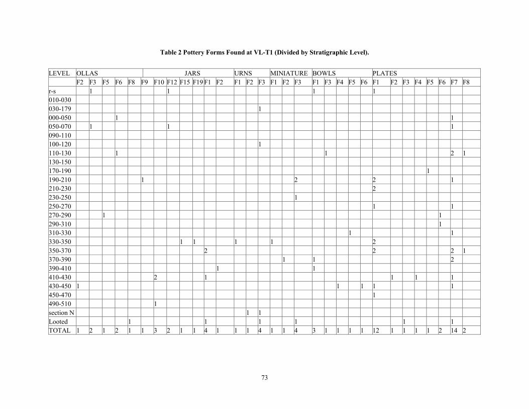
73

Table 2 Pottery Forms Found at VL-T1 (Divided by Stratigraphic Level).

LEVEL OLLAS JARS URNS MINIATURE BOWLS PLATES F2 F3 F5 F6 F8 F9 F10 F12 F15 F19 F1 F2 F1 F2 F3 F1 F2 F3 F1 F3 F4 F5 F6 F1 F2 F3 F4 F5 F6 F7 F8 r-s 1 1 1 1 010-030 030-179 1 000-050 1 1 050-070 1 1 1 090-110 100-120 1 110-130 1 1 2 1 130-150 170-190 1 190-210 1 2 2 1 210-230 2 230-250 1 250-270 1 1 270-290 1 1 290-310 1 310-330 1 1 330-350 1 1 1 1 2 350-370 2 2 2 1 370-390 1 1 2 390-410 1 1 410-430 2 1 1 1 1 430-450 1 1 1 1 1 450-470 1 490-510 1 section N 1 1 Looted 1 1 1 1 1 1 TOTAL 1 2 1 2 1 1 3 2 1 1 4 1 1 1 4 1 1 4 3 1 1 1 1 12 1 1 1 1 2 14 2

74

Table 3 Pottery Forms Found at Mound J9 of Jerusalén Site.

LEVEL OLLAS JARS URN BOWLS PLATES

F1 F2 F11 F13 F16 F17 F19 F3 F4 F1 F1 F7

r-s 2 1 1 1 1 1 1 1

100-120 1 3 1 3 1 1 1

120-140 1

TOTAL 2 1 4 1 4 1 1 1 1 2 1 2

Table 4 Pottery Forms Found at Mound Vl-T2, Vuelta Larga Site

LEVEL OLLAS BOWLS PLATES

F1 F4 F6 F7 F8 F10 F16 F18 F2 F3 F4 F1 F6 F7

r-s 1 2 1 1 1 1 2 2 3

4 1

5 3 1

6 1 1

8 1

TOTAL 1 1 3 2 1 1 1 2 1 3 1 2 3 22

75

Table 5 Frequency of Forms by Levels at Domestic Contexts (Various Housemounds)

LEVEL OLLAS BOWLS PLATES F1 F4 F6 F7 F8 F10 F16 F18 F2 F3 F4 F1 F6 F7 r-s 1 2 1 1 1 1 2 2 3 4 1 5 3 1 6 1 1 8 1 1 1 3 2 1 1 1 2 1 3 1 2 3

Vessel Function Analysis of each form category was pursued in order to define what function the vessels

would have had. We looked closely at factors such as wall thickness and overall shape. The three

main vessel functions we sought to identify were cooking or food processing, storing, and

serving (Balfet et al. 1992, Rice 1987). Hence, the sample was also divided into vessels that were

used for serving, cooking or storing, as well as urns that have funerary functions. Appendix B

indicates which forms correspond to these four functions. Both the proportions of serving and

cooking vessels as well as decorated and undecorated pottery will be discussed in later sections.

Summary

The study of ceramics in the area, although it has a long tradition, needs further refinement

to define more specific time divisions. The ceramic assemblage registered in the area corresponds

to what has been defined as Milagro-Quevedo pottery, belonging to the Late Integration Period.

At the moment all efforts to divide the 900 years of the Milagro-Quevedo phase have been

futile; as a result this study has become a synchronic analysis of the political dynamics of the

Milagro-Quevedo Yaguachi chiefdom of the Lower Guayas Basin.

76

Spatial Dimension

Procedures for Finding Sites

Any regional study, except perhaps those that are on islands or otherwise well bounded,

involves some subjectivity in defining the area to work in. Further analyses are sometimes biased

by factors like a boundary effect. Various factors are involved in the definition of an area to work

in. Archaeologists generally have tried to define a study area seeking some sort of unity,

sometimes in terms of environments, sometimes in terms of the extent of culture areas, and

sometimes in terms of the requirements of specific sampling strategies.

In this study, the area surveyed does not conform to any culturally bounded unit. The

survey focused on this area because it was clearly manageable and divided by both natural and

artificial features. The Guayas River to the west forms the natural barrier that was also present

during prehispanic times, and to the south and southeast the Boliche and Taura Rivers were used as

boundaries while at the northwest the expansion of the Durán suburbs marks the limits. Finally on

the northwest and northeast, the limits were set at the modern road connecting Milagro, Yaguachi

and Durán. Of course, in areas along the road we also tried to locate sites, but survey did not

extend farther than 100 m beyond the road. Clearly, this in no way constitutes a “culturally

bounded” unit, but it does represent part of the core of the late Yaguachi chiefly society. It

contains the still largest undestroyed sites in the region, such as Jerusalén, Cerrito Rico and La

Ensenada; in addition, it contains the largest area covered with raised fields, in the entire

Ecuadorian lowlands, as far as we know.

The study area corresponds to about 429 km² (Figure 2). A total of 32,921 shovel tests

and 940 auger holes were excavated in order to locate sites, obtain cultural material to place

those sites in time and space, and finally to understand patterns of local settlement organization.

As discussed in the methodology section, shovel tests and auger probes were placed in transects

77

100 m apart. Thus in each 1 km², 100 tests were made, but given that units contained rivers and

other features, in some units fewer than 100 tests were dug, while on others, this number

increased because site definition required using more shovel tests for defining site boundaries.

Auger coring was used in places of heavy deposition close to identified occupational

areas. Most auger holes reached 3 m deep; others stopped when waterbed table was found.

Auger testing did allow defining more accurate site boundaries, but by itself, it did not allow us

to find more sites than the ones found through shovel testing. Most times, auger coring gave the

chance to locate deeper deposits on sites already defined with shovel tests, but not a single new

site was found by auger methods only.

Site Chronology

My intention was to define a regional chronology based on excavated materials and with

that, order sites within the chronology. Then patterns for each phase would be compared to define

local settlement changes through time. Since occupation in the area belonged to only one

component, the Milagro-Quevedo phase, which, although long (900 years approximately), could

not be subdivided, there was no choice but to produce a synchronic study. Hereafter all analysis,

then, concerns the Milagro Quevedo phase, the only component present in the area.

Potential Missed Sites

In any regional survey there is the possibility that the sampling strategy failed to locate

some sites. In this case, early sites less than 100 x 100 m might fall entirely between shovel

tests. But in that case, sherds of early sites if they existed in the area should have appeared in the

many river cuts, road cuts, and deep channels dug in banana and sugar cane plantations, all of

which were examined. Taking just the 32,921 shovel tests as a sample of quadrats each the size

of a shovel test we can explore the level of statistical confidence we can have concerning the

78

presence of sites earlier than Milagro-Quevedo in the area. In effect, we ask how likely it is that

this survey missed sites earlier than Milagro-Quevedo. As Drennan (1996) indicates, a sample

size of 7,000 shovel tests that finds no material earlier than Milagro-Quevedo gives us 99%

confidence that the sample came from a population in which test with sherds of periods earlier

than Milagro-Quevedo are less than 0.1% of all the possible tests. This means that there is more

than 99% confidence that fewer than 0.1% of the total number of small quadrats the size of

shovel test that would fit into the study area have earlier sherds in them. In other words, less than

0.1% of the study area (0.1% of 429 km² =0.429 km²) has early sherds that could be found by

shovel and auger test (at the 99% confidence level). Since the sample is considerably larger than

7,000, we can extend Drennan’s approach to stronger statement. If only 0.01% of the study area

contained occupation earlier than Milagro-Quevedo, there is only a 3.7% chance that this sample

of 32,921 shovel tests would have failed to find it (0.9999 32,921). Thus we can be more than 96%

confident that there is less than 4.29 ha (0.01% of 429 km²) of occupation earlier than Milagro-

Quevedo in the study area. The chances, then, that any substantial early occupation was missed

by the shovel test sample are quite small.

It also might be that early Formative and Regional Development sites in the area are

underneath heavy levee deposition, to deeply buried to be found in shovel tests. However, it

should be noticed that Chorrera occupation at Peñón del Río started at the surface and many

deposits were only a few centimeters deep (Zedeño nd). Regional Development sites around

Guayaquil are often rather shallow and some have been found through surface survey, even the

Valdivia site reported by Gonzales de Merino (1984) cultural deposits were found at less than 50

cm below surface.

79

Site Definition

Regional analysis of settlement organization relies heavily on the notion of

archaeological site or archaeological settlement. As already mentioned the idea of exactly what

represents a site, or a meaningful unit of analysis, is much debated. Finally, the definition of site

depends on suitability to research project goals, rather than any kitchen sink list or rigid

principle. Important among factors influencing how a site is defined are the scale of analysis and

the nature of the questions asked. The question of scale is very relevant as resolution varies in

inverse proportion with the scale of analysis (DeMontmollin 1988). Focusing on household

studies one can define an archaeological site any structure, domestic or non-domestic, found

separated by considerable distance from other similar features, but, when focusing on, say,

agricultural farmsteads, the previously defined site becomes one element of a much larger site,

and this cluster of structures may be defined as part of a still larger site in a regional scale

analysis. Simply put, the notion of archaeological site is a methodological tool used by

archaeologists to organize data, an mostly the definition is arbitrary. In this research defining a

site proved to be a complicated matter; finally sites were defined by combining variables such as

clustering of mounds and cultural material evidence obtained from subsurface testing.

In surveys carried out in many parts of the world focusing on locating scatters of surface

debris, archaeologists have wondered whether surface scatters separated by a buffer area were

part of one or several sites. In such cases, determination of site size and number of sites is

difficult if separate scatters may be connected below the modern surface to form one site.

Regional surveys employing shovel tests and other probing face a similar problem in defining

what is a reliable distance between tests yielding cultural material to use in defining meaningful

site boundaries. Generally a site is defined as a cluster of tests that yield cultural remains. Areas

with high artifact density would be favored over others, such as occupational floors kept clean,

80

although checking negative tests for evidence of anthropogenic soils helps resolve this problem.

The main issue, nevertheless, is how large a buffer zone or area without signs of occupational

activity needs to be for confidently defining site boundaries.

This research, as it wrestled with this issue, used various lines of evidence; sites were

defined based on the clustering of mounds with additional information from subsurface testing.

Information on cultural activity from shovel tests and auger holes included not only the

presence/absence of artifacts, but also close examination of changes in soil color and structure.

First we tried defining sites based only on the clustering of mounds, which produced 21 sites in

the area. Adding presence of cultural material found in shovel and auger tests, road cuts and

agricultural canal cuts, reduced the number of settlements in the area to 16 as what had

previously been considered separated sites were combined (Figure 12).

Settlement Hierarchy

Exploring variables such as site area, number of mounds, mound area, total mound

volume at each site, tended to show three groups making a three-tiered settlement system

(Figures 7 through 10). One variable, mound area, forms only two groups which might be

showing differences between domestic and public mounds, or possibly differences between elite

and non elite dwellings.

81

0.00 0.25 0.50 0.75 1.00 Mounded Area

(Km²)

0

5

10

15

20

Cou

nt

0.0

0.2

0.4

0.6

0.8

1.0

1.2

Prop

ortio

n pe

r Bar

0 10 20 Site Area

(Km²)

0

3

6

9

12

Cou

nt

0.0

0.1

0.2

0.3

0.4

0.5

0.6

0.7

Prop

ortio

n pe

r Bar

Figure 7 Settlement Size based on Site Area

Figure 8 Site size based on Mound Area

82

0 50 100 150 200 250Number of Mounds per Site

0

4

8

12

16

Cou

nt

0.0

0.1

0.20.30.40.5

0.60.70.80.91.0

Prop

ortio

n pe

r Bar

Figure 9 Site Sizes Based on Mound Volume

Figure 10 Site Size Based on Number of Mounds per Site

0 50000 100000 150000 200000 Volume of Mounds (m³)

0

5

10

15

20

Cou

nt

0.0

0.2

0.4

0.6

0.8

1.0

1.2

Prop

ortio

n pe

r Bar

83

Table 6 Measurements of Local Sites

Sites Site Area m² Mound Area m2

Mound Volume m31

Number of Mounds

Cacique de Oro 1,814,473 934 1,216 4

Cerrito Rico 3,057,778 94,935 151,557 209

Druet 615,383 3,092 4,448 26

El Local 1,553,258 356 553 5

La Ensenada 856,118 14,945 51,573 59

Iguano Macho 65,960 80 160 1

Jerusalén 17,750,403 24,149 76,830 137

La Cepa 60,699 45 76 1

Quijíje 1,615,433 548 1,009 9

San José 352,733 1,308 2,028 2

San Mateo 2,497,209 1,051 6,453 3

Santa Rosa 1,111,386 1,714 2,231 5

Santay 221,398 3,776 3,764 26

Vera 178,674 622 1,790 2

Vuelta Larga 1,293,732 1,516 15,957 7

Yaguachi 12,187,997 4,098 4,352 148

1 Formulas used to calculate volume where

Irregular: 31×××= heightwidthlenghtV

Pyramidal: 31×××= heightwidthlenghtV

Circular: 312 ××= heightrV π

Elliptical: 31××××= heightwidthlenghtV π

Where π = 2.13149

84

The question now is which of the 16 sites correspond to these three groupings? Table 6

shows four variables measured for each site. This table indicates that sites can be classified in

four ways, which raises the suspicion that settlements can be classified in as many ways as there

are variables. For instance, taking the areal extent of each site, Jerusalén with 17,750,403 m²,

and Yaguachi with 12,187,997 m², are at the top of a settlement hierarchy. When using mound

area, Cerrito Rico and Jerusalén are at the top. We are faced with the problem of how to reach

an optimal classification of sites, minimizing the most important sources of bias. If we take only

the site area, settlements with dispersed dwellings are ranked higher than ones where occupation

is more closely spaced. For instance, Yaguachi, a village of many dispersed housemounds, ranks

higher than La Ensenada, which has many large mounds, but packed close together. Mound area

overcomes the bias imposed by the degree of clustering since this variable is not related to how

mounds are distributed within a site. However, by using mound area, we only have part of the

information that seems important. In this case, a site with large but low platforms will rank high,

while other sites containing high mounds will not. Mound volume provides a good measure of

site size. Another variable frequently used is number of mounds; but with this variable, a site

with many small mounds will rank higher than sites with fewer large mounds.

Site Ranking

The variables that seem least biased are mound area and mound volume. Both

measurements were used to obtain a combined ranking to form the settlement hierarchy. In

Table 6 columns 3 and 4 are site rankings for mound area and mound volume for each site

obtained from values of Table 5. Column 2 indicates the average ranking of the 16 sites.

Average rankings range from rank 16 for Cerrito Rico, to La Cepa, which ranks last. Table 7

shows three groupings, one formed by sites ranking 16 to 14 , other ranking from 11.5 to 11, and

another grouping sites ranking from 9.5 downwards.

85

Furthermore, Figure 5 shows three groups of settlements, one formed by Cerrito Rico,

Jerusalén and La Ensenada. A second group with somehow similar ranking forms sites like

Santay, Druet, Vuelta Larga, and San Mateo. These sites are almost identical in ranking, a third

group is formed by Yaguachi, San Jose, Santa Rosa, Vera, Cacique de Oro, Quijije, El Local,

Iguano Macho and La Cepa.

Table 7 Local Site Rankings

Sites Average Site Ranking

Rank Based on Mound Area

Rank Based on Mound Volume

Cerrito Rico 16 16 16 Jerusalén 15 15 15 La Ensenada 14 14 14 Santay 11.5 13 10 Druet 11.5 12 11 Vuelta Larga 11 9 13 San Mateo 11 10 12 Yaguachi 9.5 11 8 San José 8.5 8 9 Santa Rosa 7 8 6 Vera 6 5 7 Cacique de Oro 5.5 6 5 Quijije 4 4 4 El Local 3 3 3 Iguano Macho 2 2 2 La Cepa 1 1 1

86

Site Hierarchy

0

2

4

6

8

10

12

14

16

18

Cerrito Rico Jerusalen La

Ensenada Santay Druet Vuelta Larga San

Mateo Yaguachi San Jose Santa Rosa Vera Cacique Quijije El Local Iguano

Macho La Cepa Sites

Figure 11 Final Local Site Rankings (Final Ranking)

In summary, this exercise indicates, that the use of a single variable to organize

settlements in regional hierarchy is not recommended, at least for this region. Using more than

one variable makes it possible to avoid some biases. By identifying such biases we can search

for more reliable variables, especially when working with complex sites like the ones at the study

area composed of mounds of various sizes with different degrees of clustering.

Brief Site Description

The first tier in the hierarchy can be considered primary centers for political decision-

making. Second tier settlements are considered secondary centers, or sub-centers, places where

part of decision-making activities could have taken place and products could have been stored.

Third tier settlements are considered “villages” or archaeological communities inhabited by

87

mostly non-elite people, most likely functioning as agricultural villages. Here we provide a very

brief description of each site.

Primary Centers

1) Cerrito Rico

This site corresponds to a group of 209 mounds, of various forms and sizes. This complex

is found in the south of the survey area, at the southern border of the raised field area. Both public

mounds and domestic dwellings are grouped in the area. Overall, the area of the site is not very

large, but having the largest number of mounds indicates that it is a very densely packed site. The

number of mounds might actually even be larger as some classified as raised fields may well be

domestic mounds. This site lies close to the Guayas and the Taura rivers, connected by smaller

esteros. This site had not been reported until this research took place. As shown in site map

(Figure 36, Appendix A ) mounds are of various shapes and sizes.

2) Jerusalén

This site was first reported by (Meggers (1966) who described it as “Yaguachi Viejo.”

Later (Viteri Gamboa 1968) listed it along with many others in the area. The site is again

mentioned by (Buys and Muse, 1987). In that work, Jerusalén is reported as the area’s regional

center. Then, Véliz (1990) mentions it as the possible living quarters of Cacique Guayaquile.

Recently Muse considers it the primary center of the area (Muse 1991). And Stemper (1987) also

mentions Jerusalén as the largest site in the lower Basin.

Although this site has long been mentioned, no systematic work had been carried out until

this research took place. The site is the largest in the study area and has a total of 137 mounds. It

88

is formed by “barrios” with the main center at Jerusalén proper and other mounds dispersed in

different satellite clusters around the site’s main center (Figure 43, Appendix A). At the main

center, public mounds are found around rectangular “plazas.” Mound 1 at Jerusalén is the largest

and tallest in the entire region and, in conjunction with others, forms the site’s main plazas.

domestic dwellings are found towards the northeast and southwest of the main center.

3) La Ensenada

La Ensenada is close to Cerrito Rico, towards the southern border of the study area. It

consists of 59 very clustered mounds divided at the center by two local esteros (Figure 37,

Apendix A). If we consider the number of mounds and their sizes, this site has the most mounds

per unit of area. Mound 11 is unique in that it contains a ramp, which so far is the only one of that

shape found in the Lower Basin. Ramped mounds like this are more characteristic of Andean and

North Coast mounds. In general the site is very compacted; shovel tests around the site indicate

that occupation corresponds very much to the area with mounds.

Secondary Centers Second tier sites are considered secondary centers. These sites in general might have

functioned as the link between primary centers and rural settlements. Secondary centers, or sub-

centers, found in the study area are Santay, Druet, Vuelta Larga, and San Mateo.

4) Santay

Santay is located at the eastern border of Hacienda Santay, in an area close to the modern

village of Jaboncillo. It has 26 mounds packed in a small area. Mounds at this site are basically

small. The site is in the middle of a developed area where large scale modern canalization has

89

been carried out, redistributing the esteros. Local people indicate that the large modern

Jaboncillo canal corresponds to an old estero that passed approximately 30 m from the site.

5) Druet

This site is northwest of the prime center of Jerusalén and very close to it. It contains 26

mounds, all of them circular concentrated in a very small area. Most of the mounds correspond to

domestic dwellings (Figure 12).

6) Vuelta Larga

Seven mounds dispersed in a large area around the modern village of Vuelta Larga form

this site. Of those VL-T1 (Mound 1), VL-T2 (Mound 2) and VL-T3 were tested. These tests are

discussed in more length in Chapter 7, but at this point we can mention that VLT-1 corresponded

to a burial mound that has been constantly under looting attack. Here we uncovered 182 burials in

a cut carried out to clean up a profile of the mound.

7) San Mateo

This site is near the southeast of the study area, between Jerusalén and La Ensenada. It is

particularly important to note that San Mateo is the closest secondary site to the Boliche River.

Some mounds seem to have disappeared when the land was converted into a banana plantation.

This site contains the largest mound so far registered in a secondary center in the area, and Mound

2 continued to be looted as this research was carried out.

90

Rural Villages 8) Yaguachi

Yaguachi is a mounded area that encompasses an area of about 14 km² at the west side of

the Chimbo River. It is formed by a complex of 148 mounds clustered along a large riverbank. It

is located less than 400 m from the modern town of Yaguachi. In contrast to other sites in the area,

most of the 148 mounds are of small size and not very high. Judging by their morphology it is

believed that most of those mounds supported house structures.

9) San José

San José is the only site that is entirely inside the raised field zone. It is located in an area

that floods entirely during the rainy season. The site consists of two mounds and an area around

that yields material. This site is the most isolated of all and is connected to Santay, Quijíje,

Yaguachi, Cacique de Oro and Vera by the local small esteros that go into the swampy area of the

raised fields.

10) Santa Rosa

Santa Rosa is located toward the southeast of the study area, close to the Chimbo River; it

is connected to Jerusalén, la Cepa and El Local. Santa Rosa has one cluster of five mounds and a

surrounding area. Nowadays the area of the site is used for sugar cane cultivation.

91

11) Vera

Vera is located close to Quijíje, San Jose, Santay and Cacique de Oro. All these sites are

connected by a series of small esteros located around the sites. Most of the mounds at Vera are

currently in use by modern dwellers. The land around Vera is grassland used for livestock.

12) Cacique de Oro

Cacique de Oro is located in the north central zone of the study area along the estero

Jaboncillo, which connects it with Quijije and Santay. It consists of five mounds that most

probably correspond to housemounds. These housemounds are in use today, as modern

inhabitants have built their houses over the archaeological mounds. Most of the land around the

mounds has been obliterated due to the heavy use in agriculture.

13) Quijíje

Quijíje is a small cluster of four mounds and a large area around them that yields cultural

material. One of the mounds (Tola Meza) has been looted. All the mounds at this site seem to

correspond to habitations. Quijíje is connected through the Estero Jaboncillo with Cacique de Oro.

It is relatively close to Yaguachi, San José and Santay.

14) El Local

El Local is close to La Cepa and is connected to it by a small estero that during the rainy

season carries water to the Estero Mojahuevos at the south. El Local has four mounds, and the

area is now used for a banana plantation and sugar cane cultivation. The material found in and

around the mounds is located about 50 cm below surface.

92

Isolated Households

14) Iguano Macho

The Iguano Macho site has one single isolated mound surrounded by non-mounded areas.

The Iguano Macho mound is located near a small estero that connects the site with the Chimbo

River and with Santa Rosa and Vuelta Larga. The area surrounding Iguano Macho is under

cultivation by local smallholders.

15) La Cepa

La Cepa corresponds to a site classified as isolated housemounds that most likely belong to

isolated rural households. These sites correspond to Buys and Muse’s (1987) estancias. La

Cepa is close to an ancient meander of the Chimbo River. It has one single mound possibly

belonging to a domestic structure (Figure12)

The archaeological settlements in general are formed by both mounds and non-mounded

areas. Most of the mounded areas, (those that most likely supported domestic dwellings) are still

being used as platforms on which local people build their houses, protecting themselves from the

flooding during the rainy season. At the same time, local people have conveyed that building the

house on a platform protects them from serpents and in “tiempos antiguos” from crocodiles.

93

0 1 5

Kilometers

Cerrito Rico La Ensenada

San Mateo

Jerusalen

Druet

Santay

San Jose Cacique de Oro

Vera

Santa Rosa

El Local

La Cepa

Iguano MachoVuelta Larga

Quijije

Yaguachi

ArchaeologicalSites

Archaeological Sites Defined in the Lower Guayas Basin

Figure 12 Settlements Registered at the Study Area

94

Regional Demography

Previous Demographic figures Studies of demography in the Guayas basin are very sparse, and those that exist do not

use direct archaeological data. Mathewson has provided some general estimates of local

population relying on labor requirements and a unilineal evolutionary model of population

growth (Mathewson 1987a). He proposed population figures of 400,000 to 500,000 inhabiting

the larger Guayas Basin on the eve of Spanish arrival (Mathewson 1987a), basing his estimates

on measures of labor required to construct, maintain and produce the raised fields found in the

area. He assumed that 20% of the area with raised fields (20% of 500 km²) was under

cultivation, so the area supported 100,000 to 150,000 people given a population density in areas

of raised fields of 1,000 to 1,500 people per km². He then added a population of 325,000 people

for the rest of the region by assuming a density of 10 persons per km² living on non-raised field

areas. If for the sake of argument I use Mathewson’s figures, the study area would have

supported a population of 100,000 to 150,000 people.

Espinoza Soriano (1988) based on ethnohistoric data, estimates the population at 20,000

to 25,000, but it is not clear whether these figures represent the total population of the Guayas

Basin or only of the Daule chiefdom (Newson 1995).

Newson (1995) indicates that, although Oviedo describes the Guayas Basin as “bien

poblado,” Mathewson’s figures seem quite inflated. She combines the population densities

offered by Mathewson with information on the Spanish “encomiendas” to indicate that some

213,780 persons would have inhabited the interior of the Basin, using Mathewson’s 10 person

per km² density. In addition, she estimates that 25,980 inhabited the southern Basin for which

she uses a figure of 5 persons per km².

95

Population Estimates for Yaguachi The two lines of evidence just discussed provide different figures, and it is clear that they

are affected by problems of the reliability of data and of the way in which data was used. In the

case of Mathewson’s estimates, the numbers are inflated because he assumed that production

was only used for local subsistence. Such direct correspondence between population and

resources does not always work given the fact that resources can be used for trade and to

generate surplus, activities mentioned in ethnohistoric accounts. The data presented by Espinoza

Soriano and Newson might not be at all accurate, given that not every ecomendero would

provide credible information on their domains in the New World to the Spanish crown. The

archaeological evidence has biases of its own, which originate in most cases in the preservation

of the archaeological record, but there are statistical methods that can help the archaeologist to

wrestle with such issues. Here we use the archaeological evidence to obtain some rough

estimates of population at the regional level.

Naroll has observed a strong correlation between the area of occupied floors or area

under roof and population size, suggesting that population can be estimated from occupational

floors with the index of 1/10 person/m² (Naroll 1962). In our case, it is hard to estimate local

population with this method given that at this point it is impossible to determine the area that was

roofed, or the area of occupied living floors. In addition, it is likely that not everybody lived on

housemounds, and it is hard to estimate the number of housemounds that have been obliterated in

the area.

We attempted to use the burial sample excavated from VL-T1 (Mound 1) to estimate

population. In an excavated volume of 66 m³, 182 burials, including primary and secondary, were

found. Our excavation area was a small sample of the mound, some of which has been heavily

looted, but the 182 burials in 66m³ produce and average of 2.75 burials/m³. At this density, the

96

total of 1,400 m³ in the mound VL-T1 would have contained 3,850 burials, which is the total

number of people that VL-T1 must have contained. VL-T1 is, as far as we know the only burial

mound at Vuelta Larga, and we could take this number to represent all the people that lived in the

site. Given that the occupation corresponds to 900 years or some 30 generations of 30 years each,

we could estimate that about 128 persons lived in the site at any given time. The problem is that

we are not sure that all dead persons were buried in the mound or that all buried people were from

the site around it. Until this issue is resolved this demographic reconstruction is built on shaky

assumptions.

Schreiber and Kintingh (1996) observe very poor correspondence between site size and

population, but Kvamme (1997) indicates that this poor correspondence has to do with the way

data is transformed. When he uses the logarithm of site size, correspondence between site size

and population becomes quite high. In addition, Kvamme indicates that site function greatly

influences the relationship between site size and population.

A different approach to reconstructing demography from archaeological evidence was

proposed by Sanders et al. (1979) for the survey data from the Basin of Mexico. This

reconstruction came from discontent with estimates of population based on site size alone. They

suggest that: “The most direct way of estimating population of archaeological sites is to multiply

the number of house mounds (i.e. family residences) by some derived figure of mean family size”

(Sanders et al. 1979: 38). Clearly, for the Guayas Basin the same problems that prevent Narroll’s

approach apply. Sanders et al. (1979) however, provided an alternative, which is to estimate

population based on sherd density along with site size. Their method also utilizes information

from the early 16th century colonial population censuses.

97

In this research we have taken the residential density figures provided by Sanders et al., and

we have classified the sites in the lower Guayas Basin in terms of correspondence with the Basin

of Mexico numbers. These are of course, very different environments so, this approach can only

provide a rough estimate of the regional population. It is, nonetheless, important to undertake this

effort to estimate Guayas Basin populations on the basis of settlement remains rather than potential

productivity.

Table 8 Correspondence of Site Typologies of the Lower Guayas Basin and the Basin of Mexico

Lower Guayas Basin typology Sanders et al. (1979) typology

Primary Centers (core) Light-to-moderate occupation

1,000-2,500 persons/ km²

Secondary Centers and Primary Centers (periphery)

Light occupation 500-1,000 persons/ km²

Rural Villages Light-to-scanty or light occupation

500-1,000 persons/ km²

Isolated households Scanty to light occupation

200-500 persons/ km²

Having classified the sites in terms of the Basin of Mexico’s residential density typology,

the next step was to calculate each individual site’s population based on its area and then add them

up to obtain figures for the population of the region. Thus, the number of people in each individual

site was obtained by multiplying its area (in km²) by the corresponding density.

Cerrito Rico and La Ensenada are both very compact settlements so the correspondence is

straightforward. In the case of Jerusalén, it seems that the core corresponds to light-to-moderate

occupation, while the periphery corresponds to light density of occupation.

As shown in Table 9, estimates of the total local population range from a minimum of

about 26,000 persons to a maximum of about 57,000 persons. Certainly, the range is quite large but

98

with these numbers, the population of my study area in the lower Guayas Basin most likely was

about 30 to 40 thousand people.

Table 9 Estimates of Local Population Calculated Based on Sanders et al. (1979) ‘s Figures.

Site ID Area ( km²) Minimum

Population Maximum Population

Primary Centers Cerrito Rico 3.058 3,058 7,645 Jerusalén Core 2.900 2,900 7,250 Jerusalén Periphery La Ensenada

14.850 0.456

7,425 456

14,850 1,140

Secondary Centres Vuelta Larga 1.294 647 1,294 Druet 0.615 307 615 San Mateo 2.497 1,248 2,497 Santay 0.221 111 221 Yaguachi 14.187 7,094 14,187

Rural Villages Santa Rosa 1.111 556 1,111 San José 0.353 177 353 Vera 0.178 89 718 Cacique de Oro 1.814 907 1,814 Quijíje 1.615 808 1,615 El Local 1.553 777 1,533

Isolated Households Iguano Macho 0.065 13 32 La Cepa 0.060 12 30

26,585 56,905

In summary, these are not ideal estimates, but they make a starting point from which to

advance in the discussion of labor investments, the amount of production necessary to feed the

population and, the ways in which local authorities strategize about keeping people in their

domains.

99

Local Settlement Dynamics

Distance Between and Among Sites

Christaller (1966) indicates that central places will tend to be equidistant from each other,

but in our study area centers are not spatially patterned in this form. As indicated in Table 10,

Cerrito Rico and La Ensenada are found near the southern border, little more than 2 km away

from each other. Jerusalén is found to the west side, in the center of the study area, 16 km from

Cerrito Rico and 13 from La Ensenada. Second level sites are located close to primary centers:

Santay is 6 km from Jerusalén; Vuelta Larga, 6.5 km; and, Druet less than 1 km. San Mateo may

be connected to all three centers; it is 6.8 km from Jerusalén, 5.3 from La Ensenada, and 8.3

from Cerrito Rico. Third level sites are all near to secondary sites: Druet is connected with El

Local, Iguano Macho, La Cepa, and Santa Rosa; Santay is connected with Vera, San José,

Quijíje and perhaps Cacique de Oro. Vuelta Larga seems to have been connected with Vera and

Yaguachi.

100

Table 10 Distance Among Sites in the Study Area

Cac

ique

de

Oro

Cer

rito

Ric

o

Dru

et

El L

ocal

La E

nsen

ada

Igua

no M

acho

Jeru

salé

n

La C

epa

Qui

jíje

San

José

San

Mat

eo

Sant

a R

osa

Sant

ay

Vue

lta L

arga

Ver

a

Yag

uach

i

Cacique de Oro 18.01 6 6.5 16.6 2.28 7.6 6.6 1 5 13 4.8 2.4 1.3 1.7 3

Cerrito Rico 18.01 15.00 17.00 2.27 18.20 16.00 20.00 18.00 19.00 8.30 12.00 16.00 16.80 17.00 22.00

Druet 6.00 14.70 4.50 13.10 3.50 0.90 4.10 8.00 10.00 8.10 2.30 6.30 4.56 7.50 9.10

El Local 6.50 16.50 4.50 14.80 3.40 1.50 2.00 9.00 12.00 9.50 0.90 8.30 5.30 9.10 8.30

La Ensenada 16.60 2.27 13.00 15.00 15.90 13.00 18.00 17.00 18.00 5.30 16.00 14.00 15.50 16.00 20.00

Iguano Macho 2.28 18.20 3.50 3.40 15.90 5.80 3.60 5.00 8.00 12.00 1.80 5.20 1.20 5.50 6.30

Jerusalén 7.60 16.01 0.90 1.50 13.40 5.80 4.60 11.00 13.00 6.80 2.60 6.10 6.50 9.20 13.00

La Cepa 6.60 19.70 4.10 2.00 17.50 3.60 4.60 9.00 12.00 12.00 2.10 9.60 5.60 9.40 7.30

Quijije 1.30 17.90 7.80 9.00 17.00 4.80 11.00 9.00 2.00 13.00 6.90 2.30 3.60 0.80 1.20

San José 5.10 18.70 10.00 12.00 17.70 8.25 13.00 12.00 2.00 15.00 10.00 3.80 6.10 2.80 2.50

San Mateo 12.80 8.30 8.10 9.50 5.34 11.50 6.80 12.00 13.00 15.00 10.00 11.00 11.90 13.00 18.00

Santa Rosa 4.80 11.76 2.30 0.90 15.70 1.80 2.60 2.10 7.00 10.00 10.00 10.00 3.70 7.90 6.60

Santay 2.38 15.70 6.30 8.30 14.20 5.20 6.10 9.60 2.00 4.00 11.00 10.00 10.90 1.50 6.10

Vuelta Larga 1.30 16.80 4.60 5.30 15.50 1.20 6.50 5.60 4.00 6.00 12.00 3.70 11.00 3.00 5.10

Vera 1.66 17.10 7.50 9.10 16.10 5.50 9.20 9.40 1.00 3.00 13.00 7.90 1.50 2.99 5.10 Yaguachi 3.00 22.10 9.10 8.30 20.30 6.30 13.00 7.30 1.00 3.00 18.00 6.60 6.10 5.11 5.10

101

o

5

10

15

20

25

First TierSecond Tier Third Tier

Chi

mbo

Riv

er

Bol

iche

Riv

er

Gua

yas R

iver

Chi

mbo

Riv

er

Gua

yas R

iver

Bol

iche

Riv

er

Bol

iche

Riv

er

Gua

yas R

iver

Chi

mbo

Riv

er

Confidence Level

99%95%80%

Figure 13 Bullet Graphs of the Distance between Sites and Main Local Rivers

102

Political Centralization River networks and the raised field areas played key roles in determining the locations of

main centers. Cerrito Rico and La Ensenada are close to the Guayas and Boliche rivers

connecting, with the Guayas River as well. Their location on the southern border of the raised

field zone seems to indicate that their inhabitants located close to the raised fields so as to

maximize investment of labor and to protect and claim land property rights over those fields. It

is very strange that Cerrito Rico and La Ensenada are so close to each other. It is also odd that

the large Jerusalén center is located far away from raised fields, a fact that will be discussed

later. Secondary centers also do not comply with any principles of equidistant spacing; the only

patterning is that they are located close to raised fields and close to watercourses, suggesting that

they functioned as storage and distributional places. Site Druet, even though located far from

raised field zones, it is very close to the primary center Jerusalén.

Clearly, people settling zones within raised fields took part in the production and

maintenance of such agro-hydraulic features. There is no clear-cut patterning indicating the

extents of the raised field area that people at each site exploited. It can only be assured that

inhabitants of these sites exploited areas closer to their communities. Sites located within raised

field zones like Cerrito Rico and La Ensenada most likely exploited the adjacent area, but the

remaining question is how large the territory was exploited by each one of them, and more

importantly, how local people used these large areas.

Sites in the study area had a tendency to nucleate, as Table 10, shows, through nearest

neighbor analysis.

103

Table 11 Nearest Neighbor Analysis

Observed Mean Nearest Meters

Neighbor Distance 93.21

Standard Deviation 187.72

Expected (Random) mean Nearest Meters

Neighbor distance 401.07

Standard Error Expected 13.91

Nearest Neighbor Ratio 0 .23

A nearest neighbor ratio of 0.23 indicates very strong clustering and the result is highly

significant (t=22.128, p< 0.001).

Soil Fertility and Settlements

Current models of political economy indicate that in systems where chiefly power rests

on the control of agricultural resources, we expect centers of chiefly societies to be located on or

near good agricultural soils (Drennan and Quattrin 1995). If political power in the lower Guayas

Basin was tied to control of good agricultural areas, we would expect centers to locate around the

most fertile areas. Two of the three first tier sites, however, Cerrito Rico and La Ensenada are

found on Cg type soils, wet and water-saturated, and ranking lowest on the fertility scale.

Jerusalén, the other first tier site, is found on three soil types: 13.15 km² (74.5%) is on LC’dv-

Cdv soil type, which ranks highest in fertility conditions. The Cgdv soil type, which ranks high

in the fertility scale, comprises 2.96 km² (16%), while the Cg-L soil type, which ranks in the

middle, corresponds to 1.55 km² (8.7%) of the site. Second tier sites are found on two soil types:

104

San Mateo is on Cg soils which ranks second lowest in fertility, while Druet, Santay, and Vuelta

Larga are found entirely on Cg-L type soils, which rank in the middle of the scale. Third tier sites

are found on both Cg-L and Cgdv soils. Only 0.13 km² (0.09%), of Yaguachi is found on Cgdv

soils types; the remaining 13.8 km² (99.9%) is on Cg-L soils. Vuelta Larga, Quijíje, Cacique de

Oro and Iguano Macho all are on Cg-L type soils, while El Local, Santa Rosa and La Cepa are

on Cgdv soils.

Thus second tier sites are found on soils ranging from low to high fertility. Third tier

sites, those most likely corresponding to agricultural populations, are found largely associated

with soils ranking high in fertility potential. No settlements were found on the most fertile soils,

which might indicate no preference for the areas best suited for agriculture. Modern agriculture

however, is heavily practiced in these areas, and perhaps as a consequence, some sites have

disappeared.

In any event, this patterning conforms most to a political system where power did not rest

on the control of the most fertile lands. This is not to say that political power may not have

rested on the control over intensive agriculture systems which will be discussed later, but that

elites perhaps opted for using raised fields instead of taking over the lands suitable for

agriculture with less labor investment.

105

Table 12 Site Distribution with Relation to Soil Fertility

Arc

haeo

logi

cal

Site

s

LC' C

dv -C

dv

Cg-

L

Cgc

Cgd

v

Cg

Fertility Ranking* 2 3 4 5 6

Cerrito Rico x

La Ensenada x

Jerusalén X x x

Druet x

San Mateo x

Santay x

Vuelta Larga x

Yaguachi x x

Santa Rosa X

San José x

Vera x

Cacique x

Quijíje x

El Local X

Iguano Macho x

La Cepa X

1 = most fertile soil, 6 = least fertile soil

106

Cgc Soil

Cg Soil

Cgdv Soil

LC'dv Cdv Soil

Cg-L Soil

Figure 14 Map of Distribution of Settlements in Relation to Local Soils

107

Exchange Routes and Settlements

The local river system seems to have been a very important natural feature that allowed

transportation and communication, and the flow of local goods. A few decades ago, it was

possible to see large balsas (rafts) transporting goods from the pie de monte to the port of

Guayaquil. Early colonial accounts indicate the presence of major bulking places along the

Babahoyo and Chimbo rivers as well as their tributaries.

Patterning of Milagro-Quevedo settlements in the study area in relation to rivers indicates

that, although first tier sites located close to the major rivers, Chimbo and Boliche, they were

even closer to smaller esteros connecting with those rivers. Local esteros cross over all three

large settlements Cerrito Rico, Jerusalén and La Ensenada. These esteros, in the case of Cerrito

Rico and la Ensenada connect them to the Boliche River. In the case of Jerusalén, the large

Estero Mojahuevos connects this site with the Guayas River and a large raised field area. Cerrito

Rico is also located about 4 km from the Guayas River, and connected to it by local esteros as

well.

In general, second tier sites are located close to the main rivers and large esteros: San

Mateo is near the Boliche River; Vuelta Larga and Santay are found close to the Estero

Jaboncillo; while Druet is near the Estero Mojahuevos. Third tier sites are near esteros

communicating with second tier sites, and, in the case of Yaguachi, near the Chimbo River.

Vera, Quijíje, Cacique de Oro and Iguano Macho connect to Vuelta Larga thorough the estero

system. La Cepa, Santa Rosa and El Local connect with Jerusalén and Druet, while San José and

Quijíje connect with Santay and Vuelta Larga. In general all sites are connected to others

forming a real web (Figure 15).

When comparing distances to the three major rivers, the mean distance of first tier sites to

the Chimbo River is 14.43 km; to the Boliche River, 11.41 km; and to the Guayas River, 14.21

108

km. Mean distance from second tier sites to the Chimbo River is 7.34 km; to the Boliche River,

7.68 km; and to the Guayas River, 13.25 km. Mean distance from third tier sites to the Chimbo

River is 3.10 km; to the Boliche River, 11.41 km, and to the Guayas River, 14.21km. First tier

sites are located at 1.47 km from the nearest main river, while secondary sites are located 2.21

km and third tier sites locate at 3.70 km. First tier sites are more than twice as close to the main

rivers than secondary sites are. Third tier sites are the farthest away from the main rivers,

although they seem to be closer to smaller esteros through which they were connected to the

centers and subcenters.

This patterning seems to establish that site location was influenced by distance to the

local drainage system. It is also clear that the sites all connect to each through the web of esteros

and rivers in the area. Thus, we can argue that centers may have functioned as redistribution

centers, places from which trade took place. People inhabiting subcenters and rural communities

might have transported agricultural products to the centers to be redistributed and perhaps traded.

People living at the regional centers, by locating close to the main rivers might have been at an

advantage in controlling the flow of exotics in the area and thus involved in alliance building

(Muse 1991).

Subcenters are also close to the main rivers, but with the exception of San Mateo, they

are not as close as first tier sites. They are located in areas between centers and productive zones

and thus they seem to have been involved in agricultural production, perhaps through

organization of labor and in the distribution of harvest to the main centers. Third tier sites, with

the exception of Yaguachi, are placed inland, farther from the main rivers, and connected to first

and second tier sites by esteros. They are close to productive areas, and mostly on soils with

regular to high fertility. Their location seems not to have been influenced by distance to the main

109

rivers but instead by the presence of highly productive areas, or areas converted to high

productivity (this will be discussed at length in other sections). Their position farther away from

the main rivers indicates that they were less connected to the main exchange routes and thus rural

households seem not to have been directly involved in long distance exchange relations.

Table 13 Distance (in km) From Sites to the Major Local Rivers

Archaeological Sites Chimbo River Boliche River Guayas River

Cerrito Rico 20.11 1.10 3.95

La Ensenada 18.48 1.20 6.52

Jerusalén 4.71 2.11 17.50

Druet 5.50 5.30 14.91

San Mateo 14.22 0.20 14.00

Santay 6.31 14.63 10.39

Vuelta Larga 3.35 10.61 13.70

Yaguachi 0.40 15.64 12.23

Santa Rosa 2.97 6.70 17.30

San José 6.61 15.40 11.90

Vera 5.60 13.73 13.30

Cacique 2.39 14.11 12.97

Quijíje 3.90 13.40 11.20

El Local 1.60 7.10 16.79

Iguano Macho 2.70 9.20 16.06

La Cepa 1.74 7.49 19.18

110

Estero

Estero Mojahuevos

0 1 5

Kilometers

R I O

G U

A Y

A S

Rio Chimbo

Rio Milagro

Los Monos

R i o

B O L I C H E

Estero Cantagallo

R I O

G U

A Y

A S

Estero

Estero Belin

Chobo

Estero los Chirijos

Estero Timalo

Estero Guayavo

Estero P echiche

Bodeguita

Estero Boliche

E s t e r o C u m b e n c i a

Estero

Cerrito Rico La Ensenada

San Mateo

Jerusalen

Druet

Santay

San Jose Cacique de Oro

Vera

Santa Rosa

El Local

La Cepa

Iguano MachoVuelta Larga

Quijije

Yaguachi

ArchaeologicalSites

Relation of Local RiversWith ArchaoelogicalSites

0 1 5

Kilometers

Figure 15 Distribution of Sites in Relation to the Local River Network

111

Summary

In summary, site definition is not clear-cut in the region, but various lines of

complementary evidence suggest some patterns. Altogether 16 sites were defined in the area with

641 mounds of both public and domestic functions. There is an indication of a three-tier

settlement system formed by centers, subcenters and rural villages, with some isolated

households in addition. Reconstruction of local demography indicates that about 30,000 to

40,000 people occupied the area. Regional population density is low, but because sites are found

clustered, density increases at the settlements. Contrary to what was expected, large centers do

not occupy the most fertile lands, but are sometimes on the worst soils. Centers are located close

to the main rivers, supporting the assertion that people in the centers were most likely engaged in

exchange relations. Rural populations were found in the most fertile lands and farthest away

from the main rivers, supporting the idea that these people were detached from river-based

interregional exchange, and as expected were settling the most productive soils. Next we will

explore raised fields and see what were the relationships between settlements and this system.

112

C h a p t e r 6

RAISED FIELD TECHNOLOGY

Introduction

Raised field cultivation is a technological development widely used in the process of

agricultural intensification. The main characteristic of intensive agriculture is that it provides a

much larger output per unit of area than extensive systems. Intensive agriculture is tied to highly

sedentary societies since the use of this technology requires long-term activities and it often

involves water redistribution.

Raised field systems are composed of elevated surfaces and areas in between that serve as

channels where water either is drained or contained (Erickson and Candler 1989). They allow

water redistribution and consequently drain water-saturated areas, or in some cases, maintain soil

humidity. In highland areas of Ecuador raised fields are usually a water-redistributing system that

permits maintenance of soil humidity and at the same time protection from frost. In such

environments they function as means of water distribution. Conversely, in most lowland areas,

raised fields constitute part of drainage systems in areas subjected to frequent flooding. In the case

of the Guayas Basin, the use of raised field technology made possible to drain areas subject to

constant flooding. It also functioned to distribute water since maintaining water in channels for

some time holds it to fight adverse dry conditions during the dry season. In the area close to the

Guayas River, the system seems also to have combated the salinity from seawater in the Guayaquil

Gulf.

113

Raised Field Taxonomy

Geographers working with raised fields have proposed various taxonomies to identify these

features across the landscapes where they occur. Denevan ( 1982) and Denevan and Turner (1974)

offered a classification placing emphasis on overall field patterning: combed, checkerboard and

ladder patterns. Denevan and Turner (1974) also presented a three-way typology: caño,

checkerboard, and clustering of loosely parallel ridges.

Caño types were found associated with oxbow lakes in the Venezuelan Llanos (Gasson

1998), Zucchi 1979) and Colombia’s San Jorge area (Parsons and Shlemon1982, Plazas 1987).

Checkerboard patterns are found in high altitude regions, such as the Peruvian–Bolivian Altiplano

(Erickson 1989,1993) and the Sabana de Bogotá region (Broadbent 1987). Erickson (1989), found

three patterns in the Huata area of the Peruvian Altiplano: open checkerboard, riverine, and

irregular, embanked and linear. Clustering of loosely parallel ridges are found in lower areas such

as Llano de Mojos (Denevan 1966, Walker 1999) Pulltrouser Swamp (Turner 1983b), and the

Guayas Basin (Denevan et al. 1985). The list goes on and classification depending of patterning is

very diverse (Denevan 2001).

Mathewson (1983:841), in an effort to provide a more specific taxonomy, indicates that

raised field forms patterns both in aggregate and individual, and mentions that those aggregated

and individually forms seem to have a degree of association with distinct biotopes in different parts

of the New World. He places raised field taxonomy within a biotope classification formed by

riverine, swamp, marsh, savanna and lacustrine environs. Furthermore, he views riverine biotopes

as places where permanent house gardens cultivation first developed. He classified the Guayas

Basin’s raised fields in the swamp biotope.

114

Raised fields in the Guayas Basin went unnoticed for a long time. It was not until James

Parsons (1969), while landing at Guayaquil airport identified them in nearby Durán that they

become the focus of attention. After noticing them, Parsons cleaned channel cuts and collected a

sample of pottery corresponding to the early Formative Valdivia phase. On this basis, he

reported that raised fields in Durán might be the earliest found in the New World. Its association

with Valdivia pottery brought general attention, and although the accuracy of this early date has

been questioned on the grounds of unclear contextual association, his work prompted sudden

interest in the area which resulted on a number of important contributions dealing with local

raised field technology (Alvarez 1984, 1989, Buys 1987, , Martínez 1987, Mathewson 1987a,

1987b, Stemper 1993).

One of those contributions was the first systematic work conducted by Mathewson

(Mathewson 1987a, 1992) in the area of Samborondón, near Guayaquil. Although raised field

technology was the focus of that study, limited archaeological data was used to draw conclusions

about possible links (Mathewson 1987b). Perhaps Mathewson’s most important contribution is

that in addition to studying raised field technology around Samborondón, he mapped most of the

raised fields spread over the larger Guayas Basin (Mathewson 1987a) and in collaboration with

Denevan and Witthen classified them into nine zones or raised field complexes (Denevan et al.

1985). Of those nine complexes, four: the Bulu-Bulu, Chilintomo, Peñón del Río (Durán) and

Taura are located in the Lower Basin (Table 14). He claimed that the extent of the raised fields in

the Guayas Basin is about 500 km². The area of study of the present research corresponds to a

large part of the Taura and some small parts of the Peñón del Río (Durán) complex.

Two other important contributions to our understanding of raised fields in the Guayas

Basin are Stemper's study of the Colimes complex near Daule (Stemper 1987, 1993), and

115

research on the Peñón del Río (Durán) complex carried out by members of the Centro de

Estudios Arqueológicos y Antropológicos (CEAA) of Escuela Superior Politécnica del Litoral

(Alvarez 1984, 1989, Martínez 1987). Both of these studies specifically linked the use of raised

field technology to factors of sociopolitical complexity. Stemper concluded that the use of raised

field technology was essential to securing to the chiefly elite the surpluses that provided them

with resources to participate in supraregional trade networks (Stemper 1993). In Peñón del Río,

the major archaeological site has been identified as a node for distribution of staple goods from

nearby lands to main centers (Muse 1991).

In describing the specific characteristics of the overall Guayas Basin raised field

complexes (Table 14), Denevan et al. (1985: 181) stated that the Taura complex (Figure 17)

contains medium sized, circular to rectangular platform fields, with some bundles of sub-parallel,

linear ridges. Mathewson (1987b: 232) also indicated that Taura fields vary in both size and

shape with the majority being circular and nearly circular shape, with sub-parallel shapes also

evident. The adjacent Peñón del Río raised field complex, also known as Durán, contains long,

linear ridged fields, with general north-south orientations; these raised fields are long linear,

some fields are longer than 1 km (Mathewson 1987b: 231).

Since the buffer zone that separates the Taura and Peñón del Río or Durán complexes,

correspond to areas of modern habitation where ancient raised fields would be undetectable, we

will treat them as just one large complex, separated in modern times by demographic expansion.

Further mention of raised fields in this study refers to parts of the Taura and Peñón del Río

(Durán) complexes.

Departing from Denevan et al.’s (1985:181) characterization of the Taura and Peñón del

Río raised fields, a further classification was made based on the clustering of individual shapes

116

instead of an aggregate patterning. Contrary to what occurs in areas such as the Sabana de

Bogotá, Llanos de Mojos or the Lake Titicaca Basin, in the lower Guayas Basin, aggregate

patterning of raised fields is impossible to define; instead it is easier and more reliable to identify

clustering of individual shapes. Based on this classification, it was possible to define nine

clusters containing four raised field categories; these four categories corresponded to two raised

field shapes, further classified by size. The four types correspond to small rectangular raised

fields, small circular raised fields, large rectangular raised fields and large circular raised fields

(Figures 17-20). Definition of raised field zones was based on visual inspection of aerial

photographs at large scales. First, pairs of aerial photographs were observed with a stereoscope

that permitted three-dimensional views of the area’s surface. Larger raised field and large

mounds were located in this step. To identify smaller raised fields and mounds, these

photographs were scanned, and the images in digital format were enlarged to the maximum

extent possible.

117

Table 14 Distribution of Individual Raised Field Types in the Guayas Basin

Complex Location Types

Babahoyo North edge of the Lower Basin, and middle Basin

Irregular to rectangular platforms with some checkerboard patterns

Bulu-Bulu East Lower Basin Apparent ditched fields with little or no raised surface

Colimes Lower High Basin Tight checkerboard, parallel platforms within oxbows.

Chilintomo Northeast of Lower Basin and piedmont

Extremely irregular and regular rectangular platforms, possibly for specialized arboriculture.

Daule Middle Basin Irregular to rectangular platforms mostly in abandoned river channels.

Peñón del Río East Lower Basin Long linear raised fields with general north-south orientation.

Piedmont Southern Basin and Andean Piedmont

Irregular to rectangular platforms with some checkerboard patterns.

Samborondón Middle Basin Bundles of short, linear ridged fields interspaced with mounds of rectangular platforms.

Taura Southwest Lower Basin

Medium sized, circular to rectangular platform fields with some bundles of sub-parallel, linear ridges.

Taken from Denevan et al. (1985: 181)

118

Taura

Yaguachi

Milagro

Duran

Yaguachi

Jerusalen

Milagro

Taura

Rio Guayas

Yaguachi

Viejo

Rio Guayas

Km 26

Paralell

Small Parallel?

Taura Raised Field Complex

Map of Raised Fields in the Lower Guayas Basin Raised Field Area According to Mathewson (1987)

According to Denevan and Mathewson (1981)

Figure 16 Raised Fields Registered in the Area (According to Denevan et al.1985)

119

Figure 17 Local Small Rectangular Raised Fields

120

Figure 18 Local Large Rectangular Raised Fields.

121

Figure 19 Local Large Circular Raised Fields.

122

Figure 20 Local Small Rectangular Raised Fields.

123

72.39km

22.70

4.7025.180

13.11

13.680

10.134

1.58214.648

Small RectangularFiedls

Small Circular

Large Rectangular

Large Circuar

Fields

Fieds

Fields

0 1 5

Kilometers

Figure 21 Raised Field Clusters Found in the Study Area

Table 15 Measurements of Circular Raised Fields Sampled

Raised Fields Area (m²) Volume (m³)[1]

Small Circular Fields 15 2.50

Small Circular Fields 15 2.50 Small Circular Fields 16 2.67 Small Circular Fields 15 2.50 Small Circular Fields 14 2.33 Small Circular Fields 15 2.50 Small Circular Fields 133 22.17 Small Circular Fields 130 21.67 Small Circular Fields 171 28.50 Small Circular Fields 93 15.50 Small Circular Fields 55 9.17 Large Circular Fields 455 75.83 Large Circular Fields 539 89.83 Large Circular Fields 529 88.17 Large Circular Fields 432 72.00 Large Circular Fields 677 112.83 Large Circular Fields 498 83.00 Large Circular Fields 1124 187.33 Large Circular Fields 462 77.00 Large Circular Fields 404 67.33 Large Circular Fields 732 122.00 Large Circular Fields 730 121.67 Large Circular Fields 885 147.50 Large Circular Fields 488 81.33 Large Circular Fields 482 80.33 Large Circular Fields 1409 234.83 Large Circular Fields 696 116.00 Large Circular Fields 587 97.83

1[1] Volume calculations here are based on 50 cm height, which based on raised field profiles and field observations seem to represent the minimum height of local raised fields.

124

Table 16 Measurements of Small Rectangular Raised Fields.

Length (m)

Width (m)

Area (m²)

Volume (m³)

Area not cultivated (m²)[1]

5 2 10 1.67 8 4 3 13 2.17 10 4 6 24 4.00 13 5 5 26 4.33 26 5 2 11 1.83 13 6 3 17 2.83 12 7 6 44 7.33 16 4 3 14 2.33 12 4 4 15 2.50 12 4 4 18 3.00 12 4 2 8 1.33 15 5 3 16 2.67 22 4 4 15 2.50 18 3 3 10 1.67 6 3 1 4 0.67 5 2 2 3 0.50 14 2 2 4 0.67 9 7 4 28 4.67 7 6 3 18 3.00 22 4 5 24 4.00 19 5 5 27 4.50 20 4 2 7 1.17 12 6 3 16 2.67 4 7 3 18 3.00 13 9 2 18 3.00 8 7 2 13 2.17 18 8 2 16 2.67 10 6 3 19 3.17 12 4 3 12 2.00 13

1] Area not cultivated represents the area between raised fields, in other words it corresponds to channels

125

Table 17 Measurements of Large Rectangular Raised Fields.

Length (m) Width (m)

Area (m²)

Volume (m³)[1]

No cultivated area

52 3 156 26 88 86 5 387 65 89 92 4 357 60 48 26 4 112 19 52 33 6 201 34 69 31 6 177 30 58 29 8 239 40 63 46 4 201 34 89 38 10 384 64 99 22 4 92 15 49 33 4 128 21 71 18 6 113 19 32 44 6 282 47 88 86 8 714 119 120 19 7 141 24 57 25 8 188 31 72 28 4 98 16 95 33 6 210 35 71 39 7 268 45 78 42 8 344 57 88 66 5 350 58 182 72 4 295 49 99 65 2 137 23 126 54 4 211 35 123 58 3 151 25 72 36 2 83 14 88 28 3 81 14 32 73 5 358 60 88 76 4 301 50 98

126

127

1

2

34

56

7

8 910

11

1212 13

1415161718

19 1920

C. Raised Field Profile found in The Penon del Rio Vecinity.

Taken from Martinez (1987). 0 5 10 15 20 25

Centimeters

0

1.62

0

1.85

0

1.00m

Esteril

B. Cut Profile Showing Raised Field Construction Events

73.20 cm

5 m

A. Cut Profile Showing Raised Field Construction Events

Figure 22 Profiles of Local Raised Fields

128

For purposes of getting a more accurate picture of raised field distribution, the earliest

photographs that could be found were sought, since those give more accurate estimates of the

area covered by raised fields prior to late destruction.

Raised Field Patterning and Distribution

Distribution in Relation to Soils

In large parts of the study area, soils are not very well suited for agriculture in their

natural state, instead they need artificial drainage to be able to sustain agricultural production.

This makes it possible to argue that pre-Columbian inhabitants of the lower Guayas Basin

engaged in raised field construction seeking to “artificially treat” the vertic soils lacking drainage

to transform them into agriculturally productive fields. In confirmation of this notion, most

raised fields are located over soils affected by water saturation.

Table 18 Area of Raised Fields Found Within Soil Types.

Soil Fertility Type

Area containing Raised Field ( km²)

Percentage of Raised Field %

Cg 45.90 25.55Cgc 25.66 13.87Cgdv 54.57 29.19Cg-L 60.17 31.21LC-dv 0.24 0.13Total 186.54 100.00

129

Extent of Raised Field Zones

Production capabilities and labor investment are two important aspects of this research.

Reconstructing demography from the archaeological evidence and the amount of labor needed

for raised field production helps to define patterns of labor allocation. By defining the amount of

production needed to feed the regional population and comparing with production capacity

estimates, surplus production can be estimated.

The first task was to measure the area of each raised field in the entire study area, but this

proved to be too time consuming. The alternative approach was to sample some areas and

measure raised fields corresponding to the four types during the field survey and laboratory

processing phases. Length and width of rectangular raised fields and radius of circular raised

fields were measured in the field. This was done to determine area and volume of each field, and

calculating the area and volume for the samples, obtain projected figures for the total area of

raised fields.

Since determining the extent of the total area under cultivation (raised surface) required

knowing the ratio between raised surface area (cultivation area) and adjacent zones subject to

channeling, field measurements of the adjacent non-cultivated areas were also taken. Areas

surrounding rectangular shapes were easily measured in the field (Tables 15-17), but due to their

irregular shapes measuring the non-cultivated areas surrounding circular raised fields was

impossible. In this case, raised field outlines were drawn on a aerial photograph in digital format

and their areas calculated. This was done for areas with various degrees of clustering of circular

raised fields so as to get a less skewed group of figures. The ratio of cultivated/adjacent areas was

obtained by subtracting the total elevated area, or area under cultivation, from the total area of the

photograph where the fields were located. The cultivated area of small rectangular raised fields

130

represents 51.38% of the total area covered by complexes of small rectangular fields. For large

rectangular raised fields, this proportion reaches 56.86%. For small circular fields the proportion is

46.31%, while for large circular fields, it is 54.93%. The cultivated area of individual small

rectangular fields ranges from a minimum of 3 m² to a maximum of 44 m², with a mean of 16 m².

The adjacent area defined as not cultivated ranges from a minimum of 4 m² to a maximum of 26

m².

For calculating raised field volume, I have used 50 cm for the height. This represents a

volume most likely moved at every event, during construction and reconstruction activities.

Given that the flooding events in the region raise the water level about 50 cm in some areas, and

1 m in others, 50 cm is a conservative estimate the average height of construction.

Tables 19 to 22 show figures for volume of soil required to raise the cultivated surface by

50 cm. The volume of soil moved to construct the smallest raised fields to 50 cm height ranges

from a minimum of 2 m³ to a maximum of 22 m³, with a mean of 8 m³ and a standard deviation

of 4 m³.

Table 19 Measurements of Small Rectangular Raised Fields

Cultivated (m²) Not cultivated (m²) Volume (m³)

N of cases 29 29 29

Minimum 3 4 2

Maximum 44 26 22

Sum 467 383 232

Mean 16 13 8

Standard Dev 9 5 4

Variance 73 29 19

131

The cultivated area of large rectangular raised fields ranges from a minimum of 81 m² to

a maximum of 714 m² with a mean of 233 m². Non-cultivated area ranges from a minimum of

32 m² to a maximum of 182 m², with a mean of 233 m². The volume of soil needed to raise the

surface 50 cm in the large rectangular raised fields ranges from 40 m³ to 357 m³ and a mean of

116 m³, with a standard deviation of 67 m³.

Table 20 Measurements of Large Rectangular Fields.

Cultivated (m²) No cultivated (m²) Volume (m³)

N of cases 29 29 29

Minimum 81 32 40

Maximum 714 182 357

Sum 6756 2384 3378

Mean 233 82 116

Standard Dev 135 31 67

Variance 18189 953 4547

The area of cultivation of small circular raised fields ranges from a minimum of 14 m² to a

maximum of 171 m², with a mean of 61 m² and a standard deviation of 60 m². The smallest

circular raised field would have required a volume of 9 m³ and the largest took approximately 114

m³. The mean volume is 41 m³ with a standard deviation of 40 m³.

132

Table 21 Measurements of Small Circular Fields.

Area (m²) Volume (m³)

N of cases 11 11

Minimum 14 9

Maximum 171 114

Range 157 105

Sum 671 449

Mean 61 41

Standard Dev 60 40

The area of large circular raised fields ranges from a minimum of 404 m² to a maximum

of 1409 m² with a mean of 655 m², and standard deviation of 269 m². To produce a build up of

50 cm in the smallest of the large circular raised fields required about 269 m³, and the largest

required 940 m³. The mean volume required for these groups was 437 m³ a standard deviation of

180 m³.

Table 22 Measurements of Large Circular Raised Fields.

Area (m²) Volume (m³)

N of cases 17 17

Minimum 404 269

Maximum 1409 940

Range 1005 670

Sum 11129 7421

Mean 655 437

Standard Dev 629 180

133

Table 23 provides measurements of aggregate areas and volumes of local raised fields

corresponding to the total of each individual form. The first column indicates the four types of

individual raised field forms. The second column indicates the area in which each individual form

cluster is found. The third column indicates the proportion of cultivated area, which, as explained

before, was obtained from the difference between the area of the raised field elevated surface, and

the adjacent areas subject to channeling. The fourth column is the area of elevated surface

obtained from this proportion. Finally, the last column refers to the volume of earth involved in

elevating raised fields by 50 cm.

The results indicate that small rectangular raised fields represent by far the largest zone

with an area of 89.56 km², of which approximately 46.15 km² were elevated surface under

cultivation. Large rectangular raised fields cover 28.12 km², and a total cultivated surface for this

type was 16.04 km². Small circular raised fields cover an area of 40.04 km² and their elevated

surface is 18.54 km². Large circular raised fields are distributed in an area of 28.21 km of which

approximately 55 % corresponds to the area subject to cultivation. The total raised field area

corresponded to 186.5 km², while the cultivated area corresponds to 96.8 km². On average 52% of

the total raised field area corresponds to elevated surface under cultivation. These percentages are

higher than the 20% estimated by Denevan and Mathewson (1985). They are also higher than

figures presented by Knapp and Denevan (1985) for the northern Ecuadorian highlands. One

explanation is that this area appears to have the highest raised field density of the entire Guayas

Basin and higher than the northern highlands.

134

Table 23 Measurements of Raised Fields in the Study Area

Total Area (km²)

Cultivation %

Cultivated Surface (m²)

Volume (m³)

Large Circular Fields 28.73 55 15,780,000 7,890,000 Large Rectangular Fields 28.21 57 16,040,000 8,020,000 Small Circular Fields 40.04 46 18,540,000 9,270,000 Small Rectangular Fields 89.56 51 46,010,000 23,010,000 Total 186.54 52 96,300,008 48,190,000

135

Labor Estimates

Calculating labor requirements of raised field construction has become standard for

studies dealing with the use of raised fields and their relationship to societal complexity. But

most studies seek figures for raised field construction only, while raised field maintenance is

overlooked. In areas like the lower Guayas Basin, where every flooding event reforms the

landscape, initial construction of raised fields and periodic reconstruction events do not differ

much in labor requirements. After each flooding event, soils deposited into the channels have to

be added onto the raised surfaces, producing constant rebuilding. In almost no time, the labor

required for rebuilding surpasses the labor used in first construction.

Various scholars have proposed different indexes of person-days required to build given

areas of raised fields (Table 24). They mostly derive from experimental and ethnographical

research (Erasmus 1965, Erickson 1989, Mathewson 1987a, Turner 1983a). Measures of aerial

extent provide indexes of person-day/m² of labor required to construct a given area, while

volumetric indexes provide basis to calculate how many person-days are required to add a given

volume of soil to any surface. Both aerial indexes and volumetric figures are used here to

estimate broadly the amount of labor required to build the area’s raised fields; these estimates are

summarized in Table 24.

Mathewson’s (1987a: 326) experimental work conducted in the nearby Samborondón

region indicate that in a 6-hour working day, a person is able to move between 1 and 2 m³ of soil

to an average distance of 10 m . In Mesoamerica, Puleston (1977) indicates that 2.7 m³ is moved

per person per day. Measurements of soil moved by local shrimp farmers are estimated in 1.6 m³

in a 7-hour workday.2

2 This index is based on information from participant observation and interviews with local farmers.

136

In terms of aerial extension, Erickson (1993) indicates that 2,665 m² of raised field can be

constructed and maintained by a household of five persons in a year.

Table 24 Labor Investment Estimates for Raised Field Construction (Volumetric Figures)

Zone Amount of Raised Field construction per person per Day

References

Guayas Basin 1m³ dry, 2m³ wet Mathewson (1985), Denevan and Mathewson 1985)

Pulltrouser Swamp

2.7 m³ Puleston (1977)

Titicaca Basin

5 person household cultivated 2,665

m² per year

Erickson (1993)

Using Mathewson’s higher figure of 2 m³/person-day, raising the total cultivated surface

in the study area to a height of 50 cm would have taken approximately 24,095,000 (48,190,000

m³ / 2) person-days. If we consider the constraints imposed by the local climatic cycle

(Mathewson 1987: 326) the optimal time for construction would be about 100 days per year, a

time in which soils are neither totally wet nor completely dry. This means in other words that to

a working population of about 2,410 persons may have taken approximately 100 years to build

the area’s fields.

Here we face a new problem, which is that the first year’s effort went into building the

raised fields, the second year to building new fields and maintaining the ones already built the

last year, and during the third year, effort went into building new raised fields and maintaining

the ones built during the first and second years. Thus, as time passed the work put into raised

137

fields more than doubled and thus, the estimates need to be much higher than the ones just

reported.

Using the population figure of 40,000 for the area (see Chapter 5), we might estimate an

available labor force of 8,000. This labor force could construct the study area’s raised fields in

about 30 years. However, adding building and maintenance together makes labor requirements

grow in a geometric progression. These figures only confirm that the task of building and

maintaining the raised field required large inputs of labor. Looking at local population, labor is

the scarce resource that local authorities must secure in order to optimize production. Scholars

have argued that what is seen today is a aggregation of long term building episodes. Population

and length of occupation are key variables to consider. But it is also necessary to consider the

specific characteristics of particular raised field technology in the Lower Guayas Basin. The

estimated working population (see Chapter 6) for the area could have built and maintain only

1/30 of the total raised fields each year. This may well be indicating that not all raised fields

were in use at the same time. With the figures provided before, it can be estimated that about

1/30 of the raised fields were in use at the same time.

Erickson's (1993) data on long-term experiments in the Andean Altiplano, observes that

2,666 m² of raised fields were built and maintained by a household of 5 working people.

Following these estimates in the study area of 186.54 km², some 35,000 people would have been

required. These numbers fit well with the population estimates of 40,000 people for the area.

Thus we would conclude that perhaps not all raised fields were in use at the same time if

we take indexes of the labor force required to construct their volume, but if we take indexes

based on the aerial extent of raised fields all of them may have been under cultivation each year.

138

Table 25 Measurements of Potential Population that could be Supported in the Guayas Basin

Location Total Area of Raised Fields

Are Cultivated within Raised Fields

Persons that can be supported by production of 1 km² of cultivated area*

Total supported Population*

Guayas Basin 500,000 100 (20%) 1,600 (manioc) 160,000 Guayas Basin 500.000 100 (20%) 1,900 (maize) 190,000 Study Area 186.542 96.38 1,600 (manioc) 154,208 (Yaguachi) 186.542 96.38 1,900 (maize) 183,122 *Based on (Denevan 1982)

139

Number of People Raised Field Production Can Support

Table 24 provides figures of the potential population that raised field production could

support based on cultivation of maize and manioc. Denevan (1984) estimated the Guayas Basin

at 160,000 because the raised fields could support that many people with subsistence based on

manioc. There are problems with this estimate given that his calculations of total cultivated area

are only 10,000 hectares or 100 km2 for the entire Basin. But the estimate of cultivated area in

the Yaguachi study area alone is about 9,600 hectares (96.38 km²), very close to what Denevan

estimated for the entire Guayas Basin. Using the index of 16 persons per hectare or 0.01 km²

proposed by Denevan, the study area could support a total population of 153,600 persons on

manioc. The archaeological evidence, however, so far does not include the conspicuous pottery

items associated with manioc consumption (DeBoer 1996). Local vessel forms discussed in

Chapter 5 (see Appendix B) are most likely grain containers, and the adjacent Peñón del Río

fields contain maize phytoliths (Pearsall 1987), supporting the idea that the main crop was maize.

Using figures based on maize, the area could support a population of 182,400 persons.

Complementary Resources: Fauna

During the flooding season, the channels between raised fields support a large variety of

fish and other fresh water resources, which no doubt would have complemented the local diet,

resulting increments in the potential supporting population. This addition includes rich protein

sources. Results of faunal remains analysis performed by Peter Stahl (Appendix C) indicate the

presence of a relatively large proportions of Chelydrea or tortuga mordedora (snapping turtles),

as well as swamp turtles or tortuga de agua dulce (Kinosternon), and small numbers of Bufo

(toad), Lutra (water fox) and cairinia moschata (domestic duck). These species are mostly

found in local esteros and they surely inhabited channels surrounding raised fields. Swamp

140

turtles are now found along most channels in the abandoned raised field area. After the flooding

season today, most esteros and channels contain large amounts of fish, some of which can be

captured even by hand as flood waters dry up. Terrestrial fauna such as Didelphys, Cavia,

Tayassu, Manzama, Odocoileus, Lama and Sylvilagus, all found in the sample excavated, added

an important source of proteins.

Measuring Surplus

Sahlins (1972) notes that before calculating surplus, it is necessary to subtracts for costs of

production, which in the case of agricultural production correspond to material used for seeds, and

wealth used to obtain labor for the subsequent year. These costs, however, are not easily

recognizable as it is difficult to determine production used in consumption, and it is even more

difficult to quantify the volume of production exceeding consumption saved for the next

productive year. Exerting caution, I will discuss surplus in terms of percentages of the total

production.

The estimated population for the area of 40,000 people represents only between 22% to

26% of the population that the raised field system could potentially support either producing maize

or manioc. Phrasing this in different way, local population would have been able to consume about

1/4 of the total local potential production. That leaves in the worst of the cases about 70% of that

production that may well be used for activities other than subsistence of the local population. Now,

even if we assume that out of this 70% at least 40% was used in the production of the next

harvesting season, there is about 30% of potential surplus, about the same volume used for local

subsistence. This rather high volume would have produced enough incentives to the local chiefly

elite to engage in any strategy possible to gain access to such surpluses.

141

This figure may seem so large as to make it difficult to understand how this surplus could

be used without a lot going to waste. External trade might have been involved. Long distance trade

may be problematic because of the costs of transportation (Drennan 1986), but the Guayas Basin

river network provides efficient transportation and open access, for example, to groups such as the

Puná Chiefdom that inhabited the Guayaquil Gulf. Their area is rich in maritime resources, but

poor in agricultural production, providing natural “market” for lower Guayas Basin agricultural

production. But even considering this case, the production would have been to high for

consumption, tribute and trade. The logical explanation is that not all raised fields were cultivated

at the same time; perhaps they rested for a fallow period and thus the cultivated area is smaller, as

well as the volume produced.

Raised Field Spatial Organization

A wide range of arguments has been made about the social meanings of raised field spatial

patterning. Some have argued that raised fields with well-defined spatial patterning are well-

planned tasks that more likely were organized and planned by the managerial elites of centralized

ancient states (Erickson 1993). The underlying principle of this argument is that the degree of

planning indicates or reflects the level of complexity attained by their builders. Another argument

is that differences in individual shapes and aggregate patterns may indicate differences in time or

the work of different ethnic groups (Erickson 1993). In regard to craft production, top-down

administration is argued to result in some degree of standardization, usually reflected in the shapes

of produced work. Similarly, the more centralized the construction of raised fields is, the more

standardized raised field individual shapes and global patterning may become.

Within the study area, overall raised field patterning is rather chaotic; what we find is some

clustering of individual forms. Accepting for the sake of argument at this point that well planned

142

fields indicate central planning, on one hand clear absence of spatial aggregate patterning

undermines the argument that raised field construction was organized by strong central authorities,

on the other hand, the homogeneity of shapes and sizes of individual fields argues for a top-down

administration. We can go further and argue that the correspondence of central planning and top-

down administration is much clearly seen in state societies.

If again, for the sake of argument it is accepted that the presence of a variety of raised field

sizes and shapes indicates the presence of many distinct ethnic groups, the study area should

correspond to a rather homogeneous group. If differences in individual shapes indicate differences

in times of construction, then some organized spatial arrangements of aggregate raised fields

should emerge in the area. Instead, individual shapes are found clustered in areas that seem more

related to the surrounding geomorphological characteristics. In general, terms, the clustering of

large rectangular raised fields occurs in areas of major deposition, usually in the confluence of two

esteros and lower areas. Small rectangular raised fields usually are found in the relatively higher

zones. Meanwhile, circular shapes are found in areas that most of the year are under water, and

their construction seem to have followed most wetland systems where soil was piled, make islands

to win land over the swamp. In this case, the effect was not draining land, but producing buildup

to gain ground surface.

Land Ownership

One of the aims of this research was to determine whether productive units such as

agricultural communities or households maintained property rights over “defined areas of raised

fields,” which researchers call plots or pockets. Earle (1998:105) posits that in the case of Hawaii,

property rights were shown by individual stones marking boundaries or by lines of rocks dividing

raised field areas. As of now, it is impossible to argue for property division markers in the study

143

area. If there ever were physical markers other than natural features, they do not exist now. Raised

field clusters are broken into sections by rivers and esteros, using these as boundaries is very

problematic. The ever-changing watercourses would have made it impossible for people to locate

boundaries even from one year to another, not to mention over periods of 10 years or complete

generations.

The evidence does not support the idea that individual households were close to the plots

they exploited (see Drennan 1988), because the inhabitants lived in large relatively nucleated

communities. Neither is there a pattern of location like the one Stone (1996) observed in the Jos

plateau where plots become long strips in which people locate at one extreme to afford close

contact with neighbors. To the contrary most local agricultural households clustered along the

fringes of the raised field area and agricultural workers traveled to their cultivated plots.

The configuration of this pattern seems likely to correspond to a system of communal

property or perhaps chiefly elites’ domains. Further, the absence of settlements within the raised

fields and the large extent of the raised field zones do not support at this point the idea that

individual agricultural households independently and autonomously engaged in cultivating the

raised field plots. Even more strongly, the pattern fails to support the idea that individual

households constructed them independently from local chiefly authorities. Instead, the spatial

patterning supports two possible scenarios: one of communal land ownership or land ownership

by chiefly elites.

Spatial Relationship Between Settlements and Raised Fields

Up until now, I have presented and discussed the evidence of settlements and raised fields,

but the spatial relationship between the two has not been much discussed. This is an essential part

in searching for explanations of how labor invested in raised fields was organized. We know that

144

the raised field system required large working parties deployed with certain periodicity. We also

know that, as a whole the study area had a population density ranging from 63 to 133 persons per

km². We need to establish how this population was located in relation to the raised fields.

Of the 16 settlements defined, seven are located entirely in raised field zones. Two of the

five are first tier sites; one is a second tier site and 4 are third tier sites. These sites are Cerrito

Rico, La Ensenada, Santay, San José, Quijíje, Vera, and Yaguachi. While most of the sites are

found inside raised field zones, two, Santay and Yaguachi are found outside raised fields. Since

both Cerrito Rico and La Ensenada seem also to contain the largest proportion of elite dwellings

(see Chapter 7), then it seems that most elite households in the area are located in the raised field

zones, although that is not the case for households located at Jerusalén. In the northern part of the

study area, San José, Vera and Quijíje are located entirely in the raised field zone. About 2% of

Santay and approximately 71% of Yaguachi are found inside the area of raised fields. Most of

northern sites that locate near or within raised fields correspond to the third tier. This pattern is

contrary to that of the southwest region in that villages of agricultural producers do not locate

near large centers; they locate bordering the raised field zone giving support to the argument that

in this part of the study area, site location was tied more to the location of productive areas than

to the location of primary centers.

Another secondary site that is located near but not in raised fields is San Mateo, which is

found 700 m from the boundary. San Mateo is not only located close to the raised fields, but

also near the major Boliche River, allowing people living at the site to engage in distribution.

Vuelta Larga is located 1.8 km from raised fields, although there are apparently partially

destroyed fields closer. The other secondary center, Druet is located 3 km from the closest area

of raised fields. El Local, Iguano Macho, Santa Rosa, and La Cepa are third tier sites found at

145

considerable distances away. Jerusalén, the other primary center, is found far away from raised

fields; the distance between the easternmost boundary of raised field area and the westernmost

boundary of the site is 5.6 km, although there was easy access to raised fields provided by the

Estero Mojahuevos, which connects this site with the Guayas River. The Cerrito Rico mounds

are found mixed with raised fields, which leaves little doubt that the inhabitants of the site used

them. This is also the case of La Ensenada, found within the raised fields.

Summary

Overall, the information presented in this chapter indicates that there is no specific spatial

patterning dividing the area into individual raised field plots that might be the property of specific

households or small communities. This makes it hard to argue for a productive strategy of

smallholders providing surplus production to local chiefs by individually managing plots of raised

fields. Second, the area subjected to cultivation seems to have been larger than what previous

researchers have thought. A closer analysis indicated that the 20% cultivable land defined by

Denevan is much higher at least for the study area, even considering fallowing and disuse as

Denevan did. As a result, measurements of labor input and demographic calculations are higher

than the ones provided by previous researcher. Third, calculations of building, maintaining and

cultivating raised fields require close chronological control. Although we have not been able to

resolve the issue of exactly when these fields were constructed just yet, construction may well have

taken a rather long time. The complete absence of evidence of earlier settlements suggests that

their construction could have not started prior to AD 500 to 700.

At this point, the hypothesis derived from this work is that raised field construction started

in the Middle and Upper Basin around 1,000 years earlier and most likely expanded to the Lower

Guayas Basin during the late Integration Period. Chroniclers of the 16th century do not register

146

raised fields being used. If the occupation in the area is the result of the expansion of Middle Basin

groups into the Lower Basin, then we have to argue that raised field construction started at the

beginning of the Integration Period since the earliest occupation belongs to that time. In terms of

the time that it might have taken to build local raised fields, given the geomorphologic conditions,

it is very unlikely that their construction could take a long time. Nevertheless, the archaeological

evidence indicates the labor force required would have made this effort a long-term enterprise.

Local sites are located within the borders of the raised field zone and several that are not within the

border, are close to it, suggesting that the main factor accounting for site location is distance to the

raised field zone. Local raised fields generated large outputs that could potentially feed quite large

populations. These large outputs provided large food surpluses that could have been used by local

elites to engage in self-aggrandizing activities. Finally, these results undermine the idea that

individual households were in charge of local raised field production. Their spatial distribution

indicates that most households clustered in agricultural villages and around the three local centers

instead of living close by the actual plots that they farmed

147

0 1 5

Kilometers

Jerusale2

17,750,403 sq.m

Cerrito Rico La Ensenada

San Mateo

Jerusalen

Druet

Santay

San Jose Cacique de Oro

Vera

Santa Rosa

El Local

La Cepa

Iguano MachoVuelta Larga

Quijije

Yaguachi

ArchaeologicalSites

Location of Archaeological Sites

In relation to

Raised Field Areas

Raised Field Zones

Jerusale2

17,750,403 sq.m

Cerrito Rico La Ensenada

San Mateo

Jerusalen

Druet

Santay

San Jose Cacique de Oro

Vera

Santa Rosa

El Local

La Cepa

Iguano MachoVuelta Larga

Quijije

Yaguachi

ArchaeologicalSites

0 1 5

Kilometers

Figure 23 Distribution of Local Sites in Relation to Raised Fields

148

C h a p t e r 7

COMMUNAL ACTIVITIES, HOUSEHOLD ECONOMY AND SOCIAL

STATUS

Up to now we have discussed the evidence from the regional perspective, looking at how at

the regional level settlements place themselves in relation to other settlements and to key features

of the landscape. At this point there is a need to be more specific and study the same social

processes at lower scales, those of the communities and households, since it is in the interplay of

these components that social relations are produced and reproduced. A key feature in the current

research is the question of labor organization, which needs to be studied through the interplay

between the community and households. Studies of labor organization need to look at the

deployment of labor in both spheres (Deitler 2001).

For the most part studies of chiefly political economy make a clear distinction between a

public and domestic spheres. Sahlins (1972) makes the distinction between domestic modes of

production II and I, which represent the domestic and public spheres. In addition, scholars agree

that the dynamic of political economies is observed in the interaction of individuals and groups in

these two sociopolitical arenas. The key factor for the development of complex political systems is

the transformation of domestic labor into communal (Hirth 1993b). This simply means that part of

domestic labor (private) becomes alienated and used for communal (public) purposes (Kolb 1994,

Pauketat 2000, Sahlins 1972).

149

Thus, the interaction between public and private is also the interaction between the

communal based organization on the one hand and the organization at the level of the household

on the other. Consequently it is worth exploring how large or small was the labor allocation that

was deployed to activities beyond the household, since through those activities households become

engaged in a web of social relations that engages them into a communal arena. By engaging in

such relations households end up loosing some of their labor organization autonomy. In the next

section, I evaluate both public and domestic activities in order to explain how labor might have

been organized in the study area. I will try to show that most of the works were communally

oriented instead of focused on the household sphere.

Public sphere

The public sphere is the place where social prestige is acquired and negotiated, economic

entrepreneurial activities are developed and ideological systems are created, utilized and reinforced

(Blitz 1991, Kolb 1994, Milner 1998, Pauketat 1997b). The community is said to be the smallest

unit where the dynamics of the local political economy are manifested. It is at this level that

individual activities transcend their immediate household organization. This is also the arena where

the dynamics of chiefly economies seem to be manifested and contested.

Rather recently great emphasis has been placed on studying different aspects of social

organization at the level of the community (see Yaeger and Canuto 2000). This work is largely

focused on social relations of production and distribution, treating communities as the lowest

supra-household arena where social production and reproduction takes place. Some confusion

exists concerning how a community can be defined archaeologically (Pauketat 2000), since the

community can mean either ethnic ascription, or simply a geographically clustered group. A

community is a social institution to which people belong to create group identity that might not be

150

expressed at the level of the individual household. And thus, the community involves a series of

features that in combination provide a “uniqueness” that expresses group identity (Engels 1972).

Like household studies, community studies have the problem of how the social entity is

linked to physical manifestations that can be observed in the archaeological record. Since social

production beyond households can be expressed in communal ritual, communal work, and so forth,

it is hard to link a community with any particular space. Instead, communal production and

reproduction of society takes place in many spheres of interaction and situations. Discussions of

just what is the right definition of the community in archaeological perspective will probably keep

on developing. For our purposes here, instead of focusing what communities are, it is more

profitable to understand what communities do. Clearly there are activities that could have only be

carried out with a level of organization beyond the domestic sphere.

Clearly, it will indeed be hard to identify, quantify and qualify the entire range of public

activities that took place at a particular site or region. This holds true for the Yaguachi territory, but

we can identify some of the most important social activities that took place in the area and that

were developed clearly beyond the domestic sphere. Here we concentrate on activities of public

mound building, public burials, and feasting.

Public Mound Building

After close examination, public mounds were defined as those ≥ 2.5 m. These mounds

are generally large in size, but most important their top platform is rather small, which makes it

unlikely that they supported habitation structures. All of these public mounds are found at

primary and secondary centers, and they are absent from third level sites.

As shown in Figure 24, the average ratio of public mounds to domestic dwellings at sites

that contain both of those mounds is 20% to 80%. The two largest of the three main centers have a

151

proportion below average. Cerrito Rico has only approximately 8% public mounds, and Jerusalén

contains 12%. In La Ensenada, on the other hand, the proportion is about 1/3 of the mounds at the

site. At secondary centers, like Druet and Santay, ratios become 8% and 4% respectively, but in

Vuelta Larga the proportion increases to 17%. An unusual patterning is observed at San Mateo,

where actually the ratio is in favor of construction of public mounds which represent ¼ of those

present.

Some of the patterning observed in the proportions in question needs further exploration,

but at this point we see that something unusual is occurring at La Ensenada and San Mateo. First a

small sample size can provide unreliable proportions. Of all mounds registered in the study area,

however, the largest percentage (33%) is found at La Ensenada, followed by Jerusalén with 29%

and Cerrito Rico with 27%. As expected second tier settlements had smaller percentages of public

mounds, but overall San Mateo only provides 3% of the public mounds in the region, a proportion

similar to the other sites in the second tier.

152

0.00

25.00

50.00

75.00

100.00

DomesticPublic

Domestic 92.34 87.59 67.80 92.31 33.33 96.15 83.33 78.98

Public 7.66 12.41 32.20 7.69 66.67 3.85 16.67 21.02

Cerrito Rico Jerusalen La

Ensenada Druet San Mateo Santay Vuelta Larga Average

Figure 24 Ratio of Domestic and Public Mounds at First and Second Tier

What is observed at La Ensenada indicates that smaller numbers of domestic dwellings

were erected at this place, and thus, there is a larger proportion of public construction compared

to domestic, than at Cerrito Rico and Jerusalén. Such a situation and the fact that the site

contains the only ramped mound in the region could indicate that the site emphasized public

activities more than the other two local centers.

0.00

5.00

10.00

15.00

20.00

25.00

30.00

35.00

Public 27.59 29.31 32.76 3.45 3.45 1.72 1.72

Cerrito Rico

Jerusalen La Ensenada

Druet San Mateo Santay Vuelta Larga

Figure 25 Proportions of Public Mounds per Site (I and II Tier Sites).

153

In the case of San Mateo, it is the secondary site closest to the Boliche River and thus the

unusual proportion of public buildings might well be indicating some sort of site specialization on

redistribution.

Labor Investments

Turning to the amount of labor needed for moving soil to construct larger public mounds

(Erasmus 1965), the total volume of mounds 4 m or higher is 193,652 m³. Taking an average of

1.5 m³ of earthmoving per person per day means that 129,101 person-days were required for

construction. Erasmus indicates that in chiefdom societies, demands of corvee labor deployed to

communal activities are about 45 days a year (Erasmus 1965). Thus, about 2,869 individuals

could have built all the public mounds in the study area in one year. The earth moved for high

mound construction for public mounds still present in the area could have been done in about

three years by working parties of 1000 people. Working parties of 500 people could have built

the area’s public mounds in about five years. And 287 would have moved this amount of soil in

about 10 years.

These are only measurements of earth moving without the actual energy spent in the

construction of the mound, which needs to consider the fact that as the mound rises in height, so

does the effort to build it. Consequently, increases in mound height must have resulted in a

decrease of the index of earth moving in some direct proportion to the mound height. In

addition, the dynamic climatic processes with many flooding events must have eroded the

mounds' surfaces washing away large parts of the fill each year. Therefore, the amount of labor

required would have been larger as part of the fill was constantly washed away.

154

While with the current state of knowledge of the area and with current methods, it is

impossible to reconstruct the amount of labor that went into the construction of public buildings,

it is clear that amounts of labor for public construction would have been much higher than

calculations based in their volume. This labor requirement is very small compared with the one

calculated for constructing and maintaining raised fields. In any case, the construction of mound

building represented a large burden to local households. This task the local population

performed in addition to providing labor for working at local intensive agricultural systems.

Social Aspects of Mound Construction

Considerable amounts of labor were deployed to public mound building. Large mounds

like Mound 1 at Jerusalén and La Ensenada Mound 9 required very large volumes of soil.

Calculations of labor indicate that a large working force was used on such constructions. Mound

profiles obtained through cleaning of looters’ holes at mounds 2 and 3 at Jerusalén lack evidence to

indicate that complex activities were carried out at these places. These mound profiles do not

present evidence of living floors, or other activities. This fact undermines the idea that such large

investments resulted in important activities taking place at those mounds.

Pauketat (2000) indicates that in the case of Cahokia, the function of the mound itself

seems less important than the social functions of mound building. In this sense, mound building is

seen as providing the possibility to attain and enforce social and community cohesion (also see

Pauketat and Emerson 1997a, 1997b). Further, Kolb (1994) maintains that the investment of

energy in mound building reflects degrees of community bonding between commoner and elite

members through the creation and reinforcement of the dominant ideology.

Drawing on similar lines of thinking, the evidence indicates that large public mound

building was carried out at regional centers. Population concentrated around these centers and

155

participated in these public activities, very likely under the management of local elites. Here the

Yaguachi elite inhabiting the areas around the centers of Cerrito Rico, Jerusalén and La Ensenada

likely should have been able to command a large commoner population to work in mound

building. In doing so, chiefs provided “benefits” maintaining the population at work and making

them participants in his or her ritually based ceremonies. As in the American Bottom, it is not at

all hard to believe that community-based rituals were associated with mound building activities

(Pauketat 2000).

Mound building appears to have been the main corporate strategy (Blanton et al. 1996)

used by local chiefly elites to emphasize communal integration. This contradicts in part the

interpretation that network strategy was key in the political relations among local kin groups

(Muse 1991). No doubt, components of network strategies were at play as well, but the evidence

of massive public works is largely unmatched with evidence of surplus exchange so as to

consider the latter the main fuel for group solidarity and polity compactness.

Feasting Activities

The ethnographic chiefdom literature clearly shows that chiefs use many strategies to

obtain labor for public works. Important among these strategies is feasting (Hayden 1995).

Hayden (2001) indicates that through feasting, local leaders convey messages of group solidarity.

Chiefs’ prestige seems to provide the social capital that makes people want to belong to the group

close to them. In addition, this provides the context for the sanctification of authority, which goes

hand-in-hand with communal ritual activities (Dietler 20001, Kolb 1994).

Dietler (2001) and Hayden (1995, 1996, 1988) indicate the wide range of variability in

feasting activities and the multiplicity of functions that feasting has. Porter (2000) argues for the

156

existence of two main types of feasting in small-scale societies, one whose main purpose is to

integrate members and the other that is used to differentiating them. While most of what has been

discussed in the recent literature dealing with feasting has focused on feasting for differentiation,

Porter indicates that feasting is often for “integration”. According to Hayden (1995) we must

differentiate feasting activities that occur within groups and between groups, since according to

him within group feasting activities help in forming group identity and community cohesion.

It seems that as Drennan (1996) points out local chiefs strive to obtain labor and thus

most of their efforts would have been directed towards gathering people around the centers.

Consequently, the core of the feasting activities most probably sought to attract local populations

towards the centers. In addition, these feasting activities would have been most likely work

feasts, in which according to Dietler and Herbich (2001) communal hospitality is used to

orchestrate voluntary collective work. Dietler (1996) indicate that work feasting is part of a much

larger set of labor mobilization strategies. They indicate that feasting imposes obligations on

large groups of people, and through these obligations, hosts recruit labor through these feasting

activities, work parties that benefit elites are seen not as corvee labor, but instead as “collective

work events.” This provides large benefits to the chiefs, reducing tensions and discontent,

resulting in chiefly authority becoming stronger and more easily accepted.

Evidence of Feasting Activities

Communally ritualized activity through feasting most likely occurs in central places (Blitz

1993), where chiefly elites associate themselves with the larger community. Thus, the place to look

for feasting activities, public or communally based, would be central places most likely inhabited

by local leaders who were in charge of performing those celebrations (Hayden 1996, 2001). Since

the argument I am supporting is that feasting was probably the means by which local leaders

157

attracted people, and developed in them a strong sense of community, I would expect both public

places such as central plazas and perhaps leaders’ dwellings to show conspicuous evidence of

feasting.

Here we focus on the core of Jerusalén center formed by the main plaza and central

public mounds. Both in the main two plazas and adjacent areas we carried out limited testing.

The presence of such central plazas around the main “civic” center by itself may indicate the

existence of some kind of public activities, and perhaps communal feasts hosted by local chiefs.

Table 26 presents the proportions of decorated vessels occurring at the main plaza, housemound

5 at the core and housemounds at the periphery. The proportions of decorated sherds are highest

at Jerusalén’s main plaza, and much lower at the housemounds of the core and the periphery. The

main plaza also contains the highest proportion of serving vessels, with lower proportions in the

housemounds of the core area and still lower proportions in those of the periphery.

Table 26 Comparison of Proportions of Decorated Vessels and Serving Vessels between the Core and Periphery of Jerusalén (95% Confidence Level)

Jerusalén Site Decorated sherds Serving vessels

Main Plaza 42.0% ± 1.97% 56.0% ± 1.98

Core 29.0% ± 2.10% 44.0% ± 19.8

Periphery 28.0% ± 1.79% 20.0% ± 1.6

158

%

Confidence Level

99%95%80%

10

0

40

20

30

80

70

60

50

100

90

Decorated Sherds Serving Vessels

Mai

n Pl

aza

Core

Perip

hery

Perip

hery

Core

Mai

n Pl

aza

Figure 26 Bullet Graphs Showing Proportions of Decorated Sherds and Serving Vessels at Jerusalén.

159

b) Evidence of food consumption Feasting activities in general involve the consumption of large quantities of food and a

variety of exotic items, some of which are obtained from far way (Dietler 2001, Porter 2000).

Porter (2000) indicates that feasting that has the purpose of strengthening communal ties involves

the consumption of many ritualized foodstuffs. Food consumption patterns in the Jerusalén core

indicate a rather larger variety of animals consumed than those consumed at the periphery. Table

27 shows that all taxa present in either sample were among the remains at the core.

Of interest is the presence of a considerable proportion of canis in the overall sample; more

specifically these taxa have the largest proportion at the site’s core, although this may well be

related to sample size. This canis were found in direct association to public spaces like the main

plaza. We can only suggest at this point that they might have been consumed during ritual events,

and /or perhaps ritually sacrificed. Future taphonomic studies should address the issue. Guinea pig

(cavia) is found only at the core of Jerusalén, this rodent is native to the Andean region, and thus

must have been imported to the Lower Guayas Basin. Guinea pig has played an important role in

the Andean ritual and even today it is a status food item among modern Andean peasants. The

other species correspond to both terrestrial and riverine fauna mixed with some other marine items,

but overall the proportions are higher at the core of Jerusalén indicating that these sources of meat

seem to have played an important role in the feasting activities of the local Jerusalén chiefs.

For comparing differences in diversity between core and periphery, Simpson’s index was

used. This mathematical tool measures the richness and diversity of the faunal assemblage.

Richness refers in this case to the number of taxa present in the collection while diversity indicates

the proportions in which each category is present (Leonard and Jones 1989). Simpson’s index

160

provides a value from 1 to 0, the transformation 1- L provide a value of 1 for maximum diversity

and 0 for the minimum. This was obtained through the formula:

[ ])1(

)1(−

−−=∑

NNnjnj

L

Where nj = number of items in a category j and N= total number of individuals at all categories.

The diversity index of the core is 0.82 and the periphery 0.91. This shows that the faunal

assemblage from the periphery of Jerusalén is more diverse than the one at the core. But the in

the core taxa such as Canis, Chelydrea, Odocolileus and Kinosternon are present in larger

proportions. On the other hand, Cavia, Tayassu, and Didelphis are found only at the core. This

variety of foodstuffs at the center may well be showing that certain varieties of meat were

consumed only at the core of the site, and thus were probably used in feasting activities. Thus,

the periphery is more diverse. The core is dominated by three taxa , the periphery contains fewer

taxa, but the proportions of the taxa present are more even than the ones at the core and that

could be the result that for subsistence there was not much larger preferences for meat

consumption.

161

Table 27 Minimum Number of Individuals (MNI) and Proportions of Assemblage Found at Jerusalén

MNI

Canis Cavia Chelydra Odocoileus Tayassu Kinostern Mazama Didelphis Sylvilagus Bufo CairinaLutra Total Core 4 1 14 14 2 12 1 1 2 1 1 1 54 Periphery 1 0 2 2 0 4 1 0 1 1 1 1 14 Proportions Canis Cavia Chelydra Odocoileus Tayassu Kinostern Mazama Didelphis Sylvilagus Bufo CairinaLutra Core 7 2 26 26 4 22 2 2 4 2 2 2 100 Periphery 1 0 14 14 0 29 7 0 7 7 7 7 100

162

Burial Activities and Burial Patterning

O’Shea mentions six basic observations that can be made on excavated burial

assemblages. First are physical characteristics, of which sex and age are the most conspicuous.

Close examination of physical characteristics can help to define demographic patterns and

contribute to the identification of pathologies and trauma, and lead to the identification of

genetically linked groups. The second observation is preparation, which includes cremation,

inhumation posture for articulated burials and patterns of bone disposition. Detailed observation

of these features could indicate the presence of “complex” disposal programs, including ritual

mutilation, exposure, partial interment, exhumation and reburial. The third aspect is the mortuary

facility employed, involving grave shapes, dimensions, orientation and depth, which can be used

for measuring energy expenditure (Binford 1971). The fourth type of observation is of the

quantity and quality of furnishings, or the material goods associated with the dead. The fifth

observation is burial location, and the scale of archaeological analysis, be it regional, site-based,

household or individual. And finally, the sixth observation focuses on environmental factors,

which can indicate the conditions in which the burial took place.

O’Shea (1984) indicates the need for middle range theories to link certain “types of

variability to specific varieties of social behavior.” Two of the most important aspects of

mortuary variability are the amount of energy expend in burial and the pyramidal distribution of

treatments or symbols. The existence of discrete levels of energy expenditure will reflect the

existence of corresponding vertical differentiation in the living society (Binford 1971). The

pyramidal distribution reflects the fact that “positions of successfully higher social importance

are held by progressively smaller number of individuals” (Goldstein 1976)

These observations indicate two aspects or levels of analysis of burial assemblages; one

is to infer social structures involving the individuals interred and the other is to study the

163

contexts in which burials took place. Societies buried their dead, either in communal, kin-based

cemeteries or in locations near or under the dwelling the deceased lived in (Binford 1971,

Ubelaker 1981). Burial location is an important indicator of the social structure of past groups

since a public place like a cemetery, where the community by and large bury their dead most

likely corresponds to a society with strong sense of community (Gamble et al. 2001). In many

societies, burial in the communal sphere would have fostered community cohesion based perhaps

on ancestry claims.

With these principles laid out, I will turn the attention to the particular nature of the

Milagro-Quevedo burial practices and then concentrate on specific patterns of variation of an

assemblage excavated in the context of this research. This analysis will enable us to understand

better:

(a) The nature of local variability in Milagro-Quevedo burial practices in the Lower Guayas

Basin. Understanding the complexity of the burial program will reveal aspects of

both horizontal and vertical ranking3.

(b) Patterns of distribution wealth goods of local and foreign origins. This will define some

aspects of the structuring of local social ranking.

A brief assessment of what is known in regard to burial practices in the Lower Guayas

Basin societies indicates the pervasive presence of burial mounds filled with primary and

secondary burials. Most sites reported during the fifties and sixties corresponded to mounds

containing large numbers of burials (Estrada 1954, Evans 1954, Meggers 1966, Zevallos

Menendez 1995), which created the belief that all local mounds contained burials. Three types of

3 O´Shea uses horizontal ranking to differentiate with vertical ranking which refers to hierarchical positions individuals have within a

social group, horizontal ranking on the other hand refers the position social groups have among themselves, ie. kin groups, moeity,etc.

164

burials are found in these mounds. One corresponds to deep shaft “chimney” burials; a second

corresponds to burial in a single urn; and the third corresponds to grave burial without an urn

(Acuña, 1995, Evans 1954, Estrada 1954, Holm 1981, Stemper 1993, Viteri Gamboa 1968,

Zevallos Menendez 1995). Chimney burials are deposited inside an urn that is the bottom of a

stack of two to ten urns, placed upside down with their bottoms broken out, recalling a chimney

(Figures 52-53). Some interments included only a single individual, while others included

multiple individuals. Multiple burials have usually been found in urns and chimneys. Some

burials were primary, while others were secondary.

Near the Yaguachi study area, at La Elisita, Estrada (1954) reports more than forty burials,

of which more than half corresponded to single urn burials. The remaining corresponded to double

urn and multiple urn burials (Figure 41). Estrada also reported a square coffin at the center base of

the mound, thought to be the burial of a chief. Burial mounds in the vicinity indicate that perhaps

each community maintained its own burial mound, and that chimney and urn burial might indicate

differences in social status.

Burial practices seem to have occurred only in public areas. We have not found burials

associated with housemounds. Thus, we argued that burials were public activities that might have

involved complex rituals, which no doubt also contributed to maintaining communal cohesion.

The placing of bodies along with others or incorporating secondary burials with primary ones gives

some support to the idea that this task was communal rather than being performed by independent

households. In addition, the presence of primary and secondary burials and differences in the

treatment of the dead is consistent with the notions of ranking. This subject has only received

slight attention in the area thus far.

165

Based on the excavated assemblage of 182 individuals from Vuelta Larga, I will try to

provide some understanding of the patterns of burial variability, linking them to aspects of the

Yaguachi social structure. Specifically we address two main issues, one concerning with

hierarchy (Binford 1971) or ranking and the second dealing with other aspects of social

organization (Brown 1971, O’Shea 1984, Peebles and Kus 1977). The former refers to burial

variation that might indicate ethnic differences, political segments (moieties), and kin groups.

The latter refers to differences of wealth and social status, concurring with Goldstein (1976: 54)

that “ a person treated differently in death was probably also so treated in life.”

The Burial assemblage from Vuelta Larga Mound 1

As noted before, 182 individuals were identified in the VL-T1 excavated assemblage. Of

these, 104 (58%) were primary and 76 (42%) were secondary interments. Only 4 burials were

found in urns; the remaining 78 were found lying over silty fill from the adjacent area. These low

proportions of individuals in urns might be misleading because we suspect that the urns might

have contained larger number of individuals undetected because of advanced bone decay.

Secondary burials consisted of piles of dismembered individuals, or, in some cases, of a single

individual. These secondary burials contain offerings including metal ornaments, such as copper-

arsenic alloys, and copper-gold alloys, in large quantities, as well as shell beads and obsidian

artifacts.

c) Primary Burials Primary burials were not placed in urns. The total sample of primary burials consists of

104 individuals. This sample was subject to multivariate analysis searching for units of social

166

significance, including social ranking. Variables are body orientation, body position, individual age

and sex, and information on offerings (Appendix E).

d) Sexing and Aging For age determination, key diagnostic features of each skeleton were measured following

Buikstra and Ubelaker (1994). Close attention was devoted to teeth, cranium sutures and long

bone joints. The same guidelines were followed to determine individual sex where close attention

was paid to the pelvis, and within it, the sub-pubic region, the sciatic notch and skull morphology

(Buikstra and Ubelaker1994:16). For age, intervals were used: child 0-10 years, subadults (11-18),

and adults (18 and over).

The total primary burial sample contained 104 individuals: 10 are children, 10 are sub-

adults, 38 are adults and 46 are of unidentified age. These unidentified primary burials for the

most part lacked or had badly preserved diagnostic parts for accurate age determination. The

sample contains 25 males, 26 females and 53 of unidentified sex. As with age determination,

skeletons of unidentified sex usually lacked diagnostic parts, or if not, preservation was so poor

that accurate determination of sex was impossible.

e) Body Orientation Body orientation refers to the direction the upper body points to. Of the sample, 62 burials

(58%) were oriented towards the northwest; 6. representing 6% were oriented towards the

northeast; 7 (7%) were oriented toward the north; 4 (4%) toward the east; 3 (3%) towards the

southeast; and finally 1 (1%) toward the west. The remaining 28 burials, representing about 27%

are of undefined orientation.

167

f) Body Position Of the total sample of primary burials, 59 (57%) were found in an extended position with

their faces up, while 5 (5%) were found in extended position with the face down. Only one

primary burial was found with legs flexed, while 12 (12%) were found in a supine position.

Finally 3 (3%) were found in cubital position.

g) Sex and Body Orientation Of the 60 burials oriented towards the northwest, 18 (29%) are females, 10 (16%) are males

and 34 (55%) are undetermined. Of the ones whose sex was determined, the ratio is almost 1:2

meaning that in this sample, females have higher tendency to be oriented towards the northwest.

Only one male and two females are oriented toward the east, and only one male is oriented toward

the north. One male and one female are oriented towards to the northeast, and one female and one

male are oriented towards the southeast.

h) Age and Body Orientation Of the 10 children identified in the sample, 9 (90%) are oriented to the northwest and one

(10%) is oriented to the northeast. Sub-adults on the other hand seem to be randomly oriented.

i) Sex and body position Of the burials found in extended position, 7 are males, and 17 are females; one female is

found with the face down, while in the same position were found 4 males. In supine position there

were 5 males and 3 females.

Offerings

A Word on the Provenience of Local Wealth Goods

With the exception of the pottery, offerings are believed to be foreign goods. In regard to

metal, the closest production site is located in the center of the Sicán polity on the north coast of

168

Peru (Shimada 1985). Muse (1991) suggests that copper-arsenic alloy pre-forms may have been

brought from Sicán. In Peñón del Río metallographic analysis indicates that copper-arsenic

alloys were made at the site (Sutliff 1989). So far research in the Guayas Basin, and the

southwestern coast of Ecuador has not provided any evidence for local metal production. What

is certain is that the raw material is not present in the area. Shell beads are another type of

foreign material that had to be brought from the sea, where either the Manteño or the Puná

Chiefdoms maintained a monopoly on spondylus exploitation and trade (Jijón y Caamaño 1997,

Lenz-Volland 1986, Moreno Yánez 1988, Muse 1991, Volland 1995). Three quartz beads were

also found, and the only quartz workshop so far reported in Ecuador is located in the southern

highlands, in the Paute Valley (Bruhns 1987). Lastly, one obsidian blade was present and

associated with a burial, and as already mentioned, its closest source is located in the northern

Andean region of the country.

j) Copper-Gold Alloys One female adult and one male adult were found with two nose rings each of gold-copper

alloy. A third male of undefined age was also found with one earring of the same material. The

first two were oriented to the northwest, and both were adults (Burial Nos. 78 and 79), while the

third one is of undefined orientation (Burial 134).

k) Copper-Arsenic Alloys Copper-arsenic ornaments and tools are in larger number associated with males, although

some females are found with only closed rings. Tweezers, contrary to what was expected were not

found associated at all with females; instead, all 26 tweezers found with burials were associated to

males. This is also the case with rattles, of which 26 (96%) were found associated with males.

169

l) Shell Beads Shell beads were associated with both males and females, a larger number of female burials

contain shell beads. In terms of age, most burials associated with shell beads are adults; there is a

small percentage of subadults as well.

m) Obsidian Blades and Spindle Whorls One male adult was buried with an obsidian blade. One male adult and one female

subadult were found with one spindle whorl each; one female of undefined age, but within

subadult to adult range was found with three spindle whorls. Of these, the ones found associated to

females are not fired, but only sun dried.

In summary, burial practices, indicate that burying the dead was an activity that took place

in public space accompanied by ritual. Burial practices were complex, and involved the

construction of “chimneys” and the reburial and placement of cadavers in urns. Offerings

associated with the burials indicate that goods made of gold and cooper were found mostly with

males, and that both adults and subadults were associated with metal goods. This suggests a social

system based on hierarchical positions that individuals hold.

The Domestic Sphere

Households House Structures and Housemounds

The household has been said to be the smallest unit of social reproduction (Netting 1993,

1990, Sahlins 1972). It has also been defined as the social unit composed by a group of

individuals linked by kinship, co-residence and common activities (Goody 1972). In more

economic terms, a household is the minimal unit of labor pooling (Wilk and Rathje 1982).

Although a household does not equate to a family, in many cases it corresponds to an extended

or nuclear family (Bermman 1994, Wilk 1984, 1988a, 1996, 1997). In this section, I bring

170

households into the analysis to study whether they present variability in terms of wealth. Here I

want to explore whether there is evidence that indicates differential access to resources and if

that is so, I want to study the factors linked with those household access to wealth.

Household Wealth, Household Activities and Organization

The study of household wealth differences has boomed in recent years, but we still debate

what constitutes measurements of wealth in prehispanic times. While, acknowledging the many

complex dimensions that household wealth can represent in the archaeological record, most

studies agree that social differences among households are closely tied to their access to

resources (Sahlins 1972). As in modern times, precolumbian households are ranked based on

size, associated wealth, the range of activities and their location within the political system of the

larger society their members belong to. Socioeconomic differences among households have been

studied by measures of residential architecture, burial disposal, and the ubiquity and quality of

artifacts (Smith 1987). These three variables, either alone or grouped, have provided important

evidence for understanding social ranking from the household perspective (Hirth 1993b).

Scholars working in areas where house structures are still standing have noticed that one

of the clearest indicators of wealth in rural households is residential architecture (Smith 1987).

Architecture in some cases is highly displayable and durable and thus is very visible

archaeologically (Wilk 1984). It lends itself to measuring in terms of energy expenditure, to

identify larger and fancier houses (Hirth 1993b). In areas not endowed with rich and measurable

architectural remains, housefloors are important measure of social structure. Even where

housefloors are not easily recognizable or studies have not emphasized the exact definition of

house floors, the quality and quantity of goods such as decorated pottery or exotic goods have

been used to define wealth differences (Hayden and Cannon 1983, Killion 1990, Netting 1990,

Widmer and Storey 1993).

171

Data in households in the northern coast of South America are very poor; only recently

have ethnoarchaeological studies on the northern Ecuadorian coast brought attention to some of

the dynamics involving rural households (Allum 1997). Most of these studies from which

comparative evidence can be drawn indicate that local households consist of individual

structures, compared with rural compounds observed in other regions.

Since the material of which Guayas Basin houses were built did not preserve, there is no

way of exploring differences in architecture. Materials used in the area seem to have been

bamboo and perhaps wood for walls and floors, and large leaves for roofing. In consequence,

differences in material were probably not accentuated, and even so, there is no ways to pursue

this line of inquire archaeologically.

On the north coast of Ecuador (Medina 1997) indicates that the traditional form of

household composition was extended families, and their ideal location was along river banks and

near esteros. He further indicates that the typical dwelling consisted of a structure resting over

four poles with the living floors 4 m above the ground surface. A kitchen and additional rooms

can be joined to the main structure (Medina 1997). This form of construction is locally known as

barbacoas and is used by rural peasants and coastal ethnic groups like Tsachillas and Chachis.

For the most part kin-based groups cluster together in the region as with the Tsachillas (Delgado

1997b). Further, early Spanish accounts indicate that the Guayas Basin’s mounds accommodated

only one or at best a few barbacoas (Newson 1995).

House Structures, Housemounds and Households

A household is a “social unit;” materializing that social unit is not straightforward in the

sense that correspondence between household and house structure is not always warranted. Many

studies of households wrestle with this problem. Some have acknowledged it, but others have

simply not addressed the issue. Here I argue that most house structures were built on mounds.

172

Ethnohistoric information and ethnographic data indicate that for the most part one house

structure was built on each mound. Modern local peasants continue building house structures on

mounds, and they usually have one main structure with additional ones for kitchen, latrine, and

so forth.

Larger mounds can be argued to have supported a larger number of structures. This

possibility cannot be denied, but in this case, it is most likely that the extra structures were a

product of the expansion of the household, rather than a proliferation on number of households.

In the following section, I explore the distributions of (a) proportions of decorated sherds per

housemound, (b) proportions of serving vessels of housemounds at each hierarchical level, and

(c) housemound area in each tier of the settlement hierarchy. Further, I compare distributions of

items such as processing tools, obsidian, and spindle whorls. Finally, I evaluate whether total

sherd weight, the proportion of decorated sherds and the proportion of serving vessels correlate

with the area of the housemound. At the same time I explore whether households that are

located in areas of raised fields show larger variability in terms of housefloor area than the rest.

Proportions of Decorated Sherds per Housemound

In general, wealthier households would have larger proportions of decorated pottery in

their ceramic assemblages. This follows from the idea that larger labor investment goes into

producing decorated vessels which thus have higher value. Decorated vessels also correspond to

fancy ware that either is used on special occasions or shows the degree of which members to

these households were well off.

Table 28 presents data on the proportions of decorated sherds per housemound in the

area. Comparing these proportions at the tier level, we find that the first tier sites have an average

of 29 decorated sherds. It the second tier, the percentage of decorated sherds decreases to 23%, it

173

decreases even more in the third tier households, where the proportion becomes 19%. Thus the

proportion of decorated vessels decreases in direct relation to the site position in the settlement

hierarchy. As the error ranges illustrated in Figure 27 show, we can have considerable

confidence that these differences are not due simply to the vagaries of sampling.

174

Table 28 Proportions of Decorated Sherds at Local Housemounds Grouped by Tiers

I II IIISites %Sites %Sites %Cerrito Rico 21Druet 12Cacique de Oro 24Jerusalén 36San Mateo 26El Local 30La Ensenada 32Santay 31Iguano Macho 12Average 29Vuelta Larga 24La Cepa 25 Average 23Quijíje 18 San José 10 Santa Rosa 19 Vera 13 Yaguachi 21 Average 19

175

%

Confidence Level

99%95%80%

10

0

40

20

30

80

70

60

50

100

90

First Tier Second Tier Third Tier

Cerr

ito R

ico

Jeru

sale

n

La E

nsen

ada

Ave

rage

Dru

et

San

Mat

eo

Sant

ay

Vue

lta L

arga

Cac

ique

de

Oro

El L

ocal

Igua

no M

acho

La C

epa

Qui

jije

San

Jose

Sant

a Ro

sa

Ver

a

Ygu

achi

Ave

rage

Ave

rage

Figure 27 Bullet Graphs of the Proportions of Decorated Sherds Occurring at Local Sites, Grouped by Site Hierarchy.

176

Serving vs. Cooking Vessels

Among other factors that can indicate wealth, is the proportion of serving to cooking

vessels associated with local households. Larger proportions of serving vessels could indicate a

household’s involvement in feasting and thus wealth and status (Clark and Blake 1994, Hayden

1995). Usually scholars agree that wealthier households contain larger proportions of serving

vessels. With such principle in mind the sample of serving vessels associated with housemounds

was analyzed.

As Table 29 indicates, among the sites of the first tier, the proportion of serving vessels on

average is 28% vs. 72%, for cooking vessels. In the second tier, the average is only 23% serving

vessels, and at third tier sites the average is 18% serving vessels. This data supports the idea that at

centers serving activities were more frequent, supporting the assertion that wealthier people

inhabited regional centers.

Housefloor Space and Housemound Area

As explained previously, access to resources can also be marked by the size of the

household. Larger households would have better chances to engage in wider ranges of activities

and also accumulate more wealth than smaller households. One could instead, argue that larger

housemound areas could also have supported a larger number of structures and thus many

households and that size cannot be equated with household wealth. Even in modern times,

however, single structures that represent single households appear on separate mounds, regardless

of the mound size. When there is more than one structure it generally belongs to the same family

and thus members of the same household. Since here we are interested more in households than in

structures, it makes more sense to equate housemound size with household size.

177

Table 29 Proportions of Serving Vessels Associated to the Area’s Housemounds

I II III Sites % Sites % Sites % Cerrito Rico 35 Druet 22 Cacique de Oro 16 Jerusalén 26 San Mateo 37 El local 20 La Ensenada 24 Santay 29 Iguano Macho 8 Average 28 Vuelta Larga 19 La Cepa 12 Average 23 Quijíje 28 San José 18 Santa Rosa 18 Vera 18 Yaguachi 16 Average 18

178

%

Confidence Level

99%95%80%

10

0

40

20

30

80

70

60

50

100

90

First Tier Second Tier Third Tier

Cerr

ito R

ico

Jeru

sale

n

La E

nsen

ada

Ave

rage

Dru

et

San

Mat

eo

Sant

ay

Vue

lta L

arga

Cac

ique

de

Oro

El L

ocal

Igua

no M

acho

La C

epa

Qui

jije

San

Jose

Sant

a Ro

sa

Ver

a

Ygu

achi

Ave

rage

Ave

rage

Figure 28 Bullet Graphs of the Proportions of Serving Vessels Found at Each Site and Grouped by Tier.

179

Figure 29 shows that the range of variation of housemound areas at the first tier sites is

larger than the rest. These housemounds also have a large number of outliers. Housemounds

located at second tier sites have smaller areas than those found at the first tier sites, they present

fewer outliers. At the third tier sites, housemounds are still smaller in comparison with those

found at the first and second tier. Thus major variability occurs at the first tier sites, and the least

variability occurs at the third tier sites.

Figure 29 Graph Showing the Range of Variation of Housemounds Area at Each Tier Level

.

I II IIITIER

0

500

1000

1500

ARE

A (m

²)

180

Relationship between Housemound Area, Weights of Sherds, Proportions of Decorated Sherds and Proportions of Serving Vessels.

In previous sections, we found out that variation in housemound area is related to

housemound location within the tier system. Larger housemounds were found at first tier sites,

and the smallest at the third tier. Larger proportions of decorated sherds and serving vessels were

also found at first tier sites. Here we explore the relationship between those variables.

The scatter plot in Figure 30 shows that there is a correlation between housemound area

and the total weight of sherds associated to those housemounds. By the direction of the slope we

know that it is a positive correlation; as area increases so does the total sherd weight. This

correlation is moderately strong and of very high significance(r=0.592, p<0.001). This is not to

say that just that making sherd collections on larger areas will produce larger volume of sherds,

because we compared a sample of sherds from equal numbers of shovel tests associated with

each housemound.

A positive correlation of similarly moderate strength and very high significance is found

between housemound area and the proportion of decorated sherds (r = 0.62 p< 0.0001). As

Figure 31 indicates, as housemound area increases so does the proportion of decorated sherds.

181

0 500 1000 1500 2000 AREA

0

1000

2000

3000

4000

WEI

GH

T

Figure 30 Scatter Plot Measuring Sherd Weight and Housemound Area.

0 500 1000 1500 2000AREA

0

10

20

30

40

50

60

DEC

OPE

RC

ENT

Figure 31 Scatter Plot Showing the Relationship Between Housemound Area and the Proportions of

Decorated Sherds

182

0 500 1000 1500 2000AREA

0

10

20

30

40

50

60

SER

VIN

G

Figure 32 Scatter Plot Showing the Relationship Between Housemound Area and Proportions of Serving Vessels.

Household Location

Table 30 indicates the relationship between housemound and soil quality measured in terms

of fertility ranking. No housemounds were found on LCdv soil, which has the highest fertility

potential. Of those found on second rank soil, 100% correspond to housemounds at sites in the

first tier of the settlement hierarchy. Only 3.6% of the housemounds located on Cg-L soil which

ranks third are at first tier sites. On this soil, housemounds at second tier sites are 23.9%, while

those at third tier sites make up 72.5%. Of the housemounds located on Cgc soil, that ranks fourth,

100% belong to sites of the first tier. Of housemounds located on Cgdv soil, which ranks fifth,

61.8%, are in sites in the first tier, while 38.2% are at sites of the third tier. Finally, all

housemounds located on Cg soil, which ranks lowest on the fertility scale, are at second tier sites.

183

Table 30 Relation of Housemounds of First, Second and Third tier Sites with Soil Fertility.

a) Frequencies Soil Type Soil

Rank I Tier II Tier III Tier Total

LC'dvCdv 2 91.0 0.0 0.0 91.0 Cg-L 3 8.0 53.0 161.0 222.0 Cgc 4 233.0 0.0 0.0 233.0 Cgdv 5 21.0 0.0 13.0 34.0 Cg 6 0.0 1.0 0.0 1.0 Total 353.0 54.0 174.0 581.0 b) Row Proportions Soil Types I Tier II Tier III Tier Total LC'dvCdv 2 100.0 0.0 0.0 100.0 Cg-L 3 3.6 23.9 72.5 100.0 Cgc 4 100.0 0.0 0.0 100.0 Cgdv 5 61.8 0.0 38.2 100.0 Cg 6 0.0 100.0 0.0 100.0 Total c) Column Proportions Soil Types I Tier II Tier III Tier LC'dvCdv 2 25.8 0.0 0.0 Cg-L 3 2.3 98.1 92.5 Cgc 4 66.0 0.0 0.0 Cgdv 5 5.9 0.0 7.5 Cg 6 0.0 1.9 0.0 Total 100.0 100.0 100.0

* No housemounds were found over LCdv, which ranks number 1 in the fertility scale.

These patterns indicate that, while a considerable proportion of housemound, or households

of the first tier sites are located on good soils, the majority of them are found on Cgc soils, which

184

rank in the lower part of the soil fertility scale. Second tier housemounds, on the other hand, are

located on or close to soils that rank high. The same is the case for third tier housemounds which

are found primarily on Cgl soils, which rank third. First tier housemounds are larger in area, and

have higher frequencies of goods indicating wealth, but this concentration of wealth is not related

to location on high quality soils.

Housemound Area and Raised Fields

If households living in areas near raised fields were working their own plots independently

and their production was their own business, we expected that these housemounds would show

greater variability in terms of wealth indicators than those that are not near to raised fields.

Housemounds inside raised field zones are much smaller than those found outside While the

median housemound area in raised field zones is 78.6 m², the median area in the zones with no

raised fields is 162 m², more than twice the size of the area of the ones found inside raised field

zones.

As indicated by the spread of the steam and leaf (Figure 33), the range of variation of

housemound areas of those found inside raised field zones is considerably smaller than the ones

found outside raised field zones. This contradicts the idea that producers on raised fields had more

chances to become wealthier; instead it shows that local producers (those living near raised fields)

did not have larger houses. This could support the idea of a top down organization of production.

185

a) Housemounds In areas of raised fields Minimum: 12 Lower hinge: 30.1 Median: 78.6 Upper hinge: 169.1 Maximum: 936.5 0 000000111111111111111111111111111 0 H 2222222222222222222222233333333333333333 0 444444444444555555555555555 0 M 666666667777777777777 0 8888899999 1 000000000000011 1 2222222223333333333 1 44444455555 1 H 66667777777 1 88999999 2 00111 2 222223 2 44555 2 667777 2 99 3 001 3 2223 3 45 3 7 * * * Outside Values * * * 3 8 4 003345 5 145

Figure 33 Steam and Leaf Plots of Housemound Areas

b) Housemounds outside areas of raised fields Minimum: 5.2 Lower hinge: 50.8 Median: 162.1 Upper hinge: 370.3 Maximum: 1314.9 0 1111111111111111111111111111111111111111111222* 0 H 55555555566666666667777778888899999999 1 00000111111111222222233333333333333444444 1 M 5555556666677778999999 2 00111111122222223333444444 2 55556666677788899 3 0000000112222222224 3 H 556666667777788999 4 012222223333444 4 56677788899 5 112222444 5 5677799 6 00001112223 6 6799 7 011244 7 56 8 4 * * * Outside Values * * * 8 6 9 0123 11 0 12 37 13

186

Household Activities

Scholars working at the level of the household suggest that wealth differences can also

relate to the range of activities in which their members engage. To study activities, I compared the

proportions of tools, which can be assigned to particular types of activities. Table 31 shows the

frequency of tools found at sites of each level of the hierarchy. Out of all tools found at the first tier

sites, about 36% corresponds to food processing tools, while approximately 42% correspond to

obsidian tools. Spindle whorls correspond to about 22%. At second tier sites there is a big change;

food-processing tools become 87% of the assemblage while the obsidian tool proportion drops to

9%, and the proportion of spindle decreases to 4%. At third tier sites, food-processing tools are

almost the entire tool assemblage. Obsidian tools are a fraction of 1% and spindle whorls are

absent altogether. As the bullet graph in Figure 34 shows, these differences in proportions are

highly significant.

Obsidian tools were used for cutting, drilling, and other tasks involved in craft activities.

Perhaps woodworking or, shell and bone crafting were among these crafts. There was clearly

much more of such activities at first tier sites than at second and third tier settlements. In many

northern Andean societies cloth production was a very important activity and many argue that

textiles were items of wealth and important for alliance building (Langebak 1992). Here I take

spindle whorls to indicate the presence of cloth production. This activity was also heavily

concentrated at the first tier sites. At the other end of the hierarchy, food processing was the

overwhelmingly dominant activity at third tier sites.

187

Table 31 Frequency of Various Tools at Each Hierarchical Level

Tools I Tier II Tier II Tier Total Food Processing 54 179 400 633 Obsidian 62 18 1 81 Spindle whorls 33 8 0 41 149 205 401 755 Column Proportions Food Processing 36.24 87.32 99.75 Obsidian 41.61 8.78 0.25 Spindle whorls 22.15 3.90 0.00 Total 100.00 100.00 100.00

188

%

Confidence Level

99%95%80%

10

0

40

20

30

80

70

60

50

100

90

First Tier Second Tier Third Tier

Cer

rito

Ric

o

Jeru

sale

n

La E

nsen

ada

Ave

rage

Dru

et

San

Mat

eo

Sant

ay

Vue

lta L

arga

Cac

ique

de

Oro

El L

ocal

Igua

no M

acho

La C

epa

Qui

jije

San

Jose

Sant

Ros

a

Ver

as

Ygu

achi

Ave

rage

Ave

rage

Figure 34 Bullet Graphs Showing the Proportions of Decorated Sherds at Sites Grouped by Tier

189

%

Confidence Level

99%95%80%

10

0

40

20

30

80

70

60

50

100

90

Food Processing tools Obsidian Tools Weaving tools

Firs

t Tie

r Site

s

Seco

nd T

ier S

ites

Seco

nd T

ier S

ites

Seco

nd T

ier S

ites

Third

Tie

r Site

s

Third

Tie

r Site

s

Firs

t Tie

r Site

s

Firs

t-Tie

r Site

s

Figure 35 Bullet Graph Indicating the Proportions of Tools in the Material Recovered in the Area

190

Table 32 shows the distribution of utilized flakes, which represent tools, and non-utilized

flakes, in which I have included debitage and pre-forms, and finally nodules. These three

categories constitute stages in the production process and thus the presence of the three indicates

that at least the last stages of the productive process took place in the study area.

Table 32 Distribution of Obsidian Tools and Unfinished Fragments Associated with Housemounds

Obsidian Distribution

a. Frequencies (n) I II II Total Utilized flakes 62.1 18.0 1.0 81.0 Non Utilized 33.0 2.0 0.0 35.0 Nodules 3.0 3.0 0.0 6.0 Total 98.1 23.0 1.0 b. Column Proportions Utilized flakes 63.3 78.3 100.0 Non Utilized 33.7 8.7 0.0 Nodules 3.0 13.0 0.0 100 100 100

There is a larger proportion of tools than of non-utilized flakes and nodules everywhere.

That might indicate that only the last stages of production took place locally. It could also indicate

that due to the scarcity of raw material, not much was left unused. Comparing the proportions of

non-utilized flakes, the larger proportion in the first tier sites indicates that obsidian tool production

largely occurred at these sites, and at the other extreme of the site hierarchy (third tier sites), no

production seems to have taken place.

191

Household Variability

The evidence presented here indicates that housemounds found at the first tier sites are

the largest of the entire study area. They also contain larger proportions of decorated sherds and

serving vessels. As indicated before, I take larger housemounds to correspond to larger

households. Based on Netting’s claims I argue that the correspondence between larger

housemounds and a wider range of activities demonstrates that larger households carried out a

wider range of activities. These larger households most likely correspond to the wealthier ones

since as Netting (Netting 1993) argues, households become wealthier by expanding their labor

pool in order to perform wider range of activities.

Summary

This chapter has focused on sociopolitical organization and domestic economy, by studying

evidence related to communal activities and household variability. The evidence from public

activities, such as mound building, burial practices and feasting indicates that emphasis was placed

at the level of the community. Social organization was apparently characterized by strong

communal identity constantly reinforced by local chiefs through ritual activities involving large

feasting events. These ritual activities would have worked to the benefit of an elite, but not in as

direct a way as Hayden (2001), and Dietler (2001) conceive. Public mound building would also

have worked to integrate the community through participation in communal activities that provided

direct benefit to the community at large, since local chiefs seem not to have resided on these

mounds. Public burial mounds would also have contributed by connecting people with particular

places and thus reinforcing the sense of community. The sophisticated local burial program

indicates a complex array of structure that needs further analysis, but burial mounds are high

enough to be seen by most people, and their presence in everyday life would also have contributed

192

to a strong sense of community. In this way, as Porter (2000) argues, local people might have

willingly devoted their labor power to the community. The chief might, of course, have used this

willingness of the people to further his/her own interests.

The first tier settlements seem to have been the places where most non-agricultural

activities took place. Households close to the main plazas were most likely inhabited by the chiefly

elite. This is the case of mound J9, where there is clear evidence of obsidian tool making and cloth

production. The small range of variability that materials associated with rural households suggest

that agricultural production was organized at the level of the community. The small differences

between housemounds located in raised field areas and those far from them indicate that that raised

field production had little to do with competition for wealth among commoners. Given the

potentially large return that these raised fields have, we expected that households close to the

raised field zones might show substantial wealth differences and turned out not to be the case.

193

C h a p t e r 8

CONCLUSIONS

THE YAGUACHI CHIEFDOM POLITICAL ECONOMY

As stated at the beginning of the text, this research was conducted seeking to understand

the characteristics of the local political economy involving agricultural production using raised

field technology. The main emphasis was on finding evidence to reconstruct the way in which

local labor was organized. This has allowed us to present a model of sociopolitical organization

during the late Integration Period in the territory of the ethnohistoric Yaguachi chiefdom. To do

this, I explored three main lines of evidence which resulted from analysis at three different

scales: the region, the community and the household.

The underlying structure of this research was the contrast between two models of the

roles that elites and non-elites have in any complex political system. The top down view assume

that levels above that of the household are in charge of managing works such as raised fields,

while a bottom up view is the opposite. Such dichotomy provides a heuristic tool for assessing

how far in either of the two extremes the organization of raised field production in the Yaguachi

chiefdom really was.

Local Cultural Development

Before turning to how the system was organized, it is necessary to consider the local

cultural history. This work has not provided evidence for the kind of diachronic study that could

help us to understand how complexity arises in the area and what relations raised field

production had to it at earlier stages. Results of the survey included no sites earlier than the Late

194

Integration Period (AD 750-1450), even tough; the methodology applied various strategies to

look for earlier sites. While it is impossible to be 100% sure that there are not earlier sites in the

surveyed region, we have a high level of confidence that the amount of occupation, if it existed

at all, was very small. In nearby Peñón del Río, there is evidence of early Formative occupations

(Muse 1991, Zedeño nd). As mentioned in Chapter 3, Gonzáles de Merino (1986) indicates the

presence of a Valdivia occupation few kilometers from the eastern boundary of the study area

close to the modern town of Milagro. In the study area, however, no such sites have been

located.

It seems then, that this area was inhabited only fairly late by expanding populations at the

beginning of the Integration Period. In the case of Peñón del Río, the Chorrera occupation might

be related to a tradition of sites located along the Babahoyo riverbank. (Evans 1954 1957). This

occupation is not seen across the larger area. In nearby Peñón del Río as well, Martínez ( 1987)

claims to have found an association between Regional Development pottery and raised fields.

She thus claims that raised fields might have been constructed and used during that Period. The

evidence to support that claim seems very small. It seems most likely that Formative Chorrera

and Regional Development groups inhabited the shoreline of the Babahoyo River and

occasionally wandered into nearby inland regions. Then in the Integration Period, a new cultural

tradition expands from the Middle Basin.

To support this claim we can look at the variation in local Integration Period settlements.

For instance in the Upper Basin (Guillaume-Gentil 1994, 1996, 1998) the Integration period

mounds are the accumulation of construction that started in Late Valdivia times. In the region

close to Daule, Stemper, (1993) suggests that raised field use and perhaps mound building started

during the Regional Development Period. In the middle Basin, Acuña (1995) showed that

195

Integration Period burial mounds were the result of a process that started in the Regional

Development Period. Further, the ceramic assemblages from the middle and upper basin at least

in the late Periods show a wide range of differences such that Estrada (1957b) divided the period

into Milagro and Quevedo. All this evidence provides support for the assertion that the cultural

tradition studied in the Lower Guayas Basin was formed elsewhere, and that understanding the

early stages of the relationship between raised field technology and chiefly formation should be

studied in the Middle or Upper Basin.

The Yaguachi Use of Raised Fields

In Chapter 6 I indicated the existence of controversy over when raised field agriculture

appears in the area. Since raised fields cannot exist without a population to build and maintain

them, we have argued that their construction and use was a late phenomenon. Nevertheless, lets

explore once again contrary positions. Marcos (1986) has argued that this technology might have

been in use since the Formative based on the Chorrera occupation at Peñón del Río. If that were

the case, then we should find many Chorrera communities such as the one at Peñón de Río

associated with the large Taura system. As discussed previously, while it is impossible to be

absolutely certain that there is no Chorrera occupation at all, our sample allows us to be

extremely confident that Chorrera occupation, if existed was tiny. Stemper (1993) suggests the

use of raised fields in Daule region starts during the Regional Development period. We are also

highly confident that no substantial Regional Development Period occupation occurs in the

Yaguachi study area. This evidence allows us to suggest that the Yaguachi chiefdom in the area

was the result of the expansion of Milagro-Quevedo groups from the Daule region or elsewhere

in the Middle Basin towards the lower, more inundated and less hospitable terrain. These groups

succeeded in “conquering the swamp” and as a result this chiefdom became one of the most

196

important in the area. Further analysis of stylistic relationship between Middle and Lower Basin

ceramics could help us to define the viability of this hypothesis.

Signatures of Local Organization

In Chapter 2, I presented a series of archaeological expectations derived from the

centralized or top-down model and from the household autonomy or bottom-up view. These had

to do with the way in which settlements organize themselves on the landscape, and this aspect of

the expectations was assessed through a regional analysis. In addition activities at the centers

were examined through the analysis of labor allocation in the local community, based on a

comparison between core and periphery at the Jerusalén site. At the level of the household I

looked for the degree of nucleation, variability in activities at different settlement tiers. In

addition, I explored the range of public activities and variability in the burial assemblage.

Settlement Organization

The area contains a site hierarchy composed of three levels with (a) centers, (b)

subcenters or secondary sites and (c) third level sites consisting of agricultural villages and

isolated households. Three centers occur in the area, and as far as presently available

information indicates, they are contemporaneous. They seem linked to each other. Distances

between them are within a day’s walk, and if we consider traveling by rivers this distance

becomes shorter. While Cerrito Rico and La Ensenada are located on the border of the raised

field zone, Jerusalén is about 4 km away from them.

The centers are close to the main river systems and thus their location seems to be

influenced by accessibility to networks of external exchange. The placement of Cerrito Rico and

La Ensenada close to the Guayas River, which is the main connection to the open Pacific

shoreline seems to have been key in that it allowed chiefs inhabiting those sites to directly

197

oversee exchange activities with nearby societies like the Puná and Túmbez to the west and

south and the Manteño-Huancavilca to the north. In addition, Jerusalén´s placement close to the

Chimbo and Boliche rivers seem to have been key in managing trade activities with eastern

regions such as the Cañari in the Cuenca region and other Milagro–Quevedo groups closer to the

pie de monte.

At all three centers there is conspicuous evidence of public buildings. In Jerusalén the

site core is formed by large mounds surrounding plazas. These large mounds, according to the

tests carried out, seem unlikely to have been residential. Moreover, there is lack of evidence of

much ritual and public activities on the top of the mounds. The larger proportions of serving

vessels and decorated sherds at the primary centers indicate that at those centers public activities

took the form of ceremonies. In addition, evidence from Jerusalén indicates that in the core

zone, the proportion of serving to cooking vessels was the largest. Evidence of consumption of

meat from long distances and the fact that such meat had high status in the area from which it

came support the idea of feasting. On the other hand, the frequency of dog remains, perhaps

eaten, supports the idea of ritualized feasting.

Feasting activities that took place at the centers would take the form of work parties that

Dietler (2001) recognizes as part of strategies for obtaining labor. These activities, which I

argued involved a large part of the local population, served to cement the idea that mound

building and perhaps raised field construction and maintenance were for the well being of the

community. Such activities more like the modern Minga and Faena are indeed constructed

under the idea that it is communal and thus it is for everyone’s benefit. This sense of

communality would have been the perfect political opportunity for the chiefs, in that

198

communality could further their aggrandizement activities. Non-elites discontent would be

minimized and chiefly persuasion greatly simplified.

We concur with Drennan’s observation that the scare resource for surplus mobilization

seems not to have been land, but instead labor (Drennan 1987b, 1995a). Even if we accept the

most liberal estimates of population in the area, we must agree that it is not large and thus it

seems that ample resources were available.

The overall tendency to nucleation around centers and villages gives support to the idea

that chiefs attracted population towards the centers and towards clustering agricultural

households. At the same time, this nucleation that seems to have pulled people away from the

lands that they cultivated does take support away from the idea that the large raised field area

was the property of individual households ( see Drennan 1988, Stone 1991).

The second level of the hierarchy is formed by sites that do not contain such a large

volume of mound construction, and have no public mounds. These settlements seem to have

engaged in some feasting but on a much smaller scale than at the first level sites. Most of them

are located in areas between regional centers and between those regional centers and the third

level sites, which supports the idea that they represent nodes of distribution of both agricultural

production and perhaps wealth goods. Production could have been stored in the second tier sites

and then sent to the main centers with goods to finance production coming back in return. Third

level sites are of two types, nucleated rural villages and isolated farmsteads. Their placement on

the landscape shows that both agricultural villages and isolated farmsteads seem to be under the

rule of a center, either through the mediation of a secondary center or directly from the primary

center.

199

A hydrological web connects almost every single site to all others. Such rivers and

esteros provided the structure for well-established systems of communication, transportation and

redistribution in the area.

Intensive Systems

The evidence presented in Chapter 6 indicates that construction of the raised field

systems required large amounts of labor that seem to have been extracted from the household

pool. The dynamic nature of the system in the region creates the needs for large numbers of

people working for short but recurring events. These were probably much more frequent during

El Niño events.

The lack of early sites in the region allows us to conclude that these fields were built

rather rapidly and thus involved large amounts of labor power. The absence of clear boundaries

and “well defined patterning” argues that most likely the local communities that formed the

Yaguachi chiefdom used the entire raised field area. Clearly the production of these systems was

large and provided the opportunity for local chiefs to engage in wealth accumulation.

Communities and Households

In Chapter 7 I established that the community was the arena where household labor was

transformed and in this process households, lose their organizational autonomy. In the Yaguachi

area, public mound building and feasting seem to have been strategies utilized by local chiefs to

draw people to the center and thus maintain a larger population subjected to them.

In addition, communal burial practices that incorporated mound-building and re-burial

must have worked as an important factor in bonding together members of the community. Large

mounds with burials inside would have encouraged development of strong communal sentiment

and ties (Pauketat 2000, Pauketat 1997b). In times of turmoil, for instance, reburial and mound

building could have been used to challenge public discontent (Kolb 1994).

200

n) Households Among the archaeological signatures for top-down and bottom-up models were patterns

of wealth variation at the level of the household. In the bottom-up model, rural households will

tend to locate near their plots and show a large range of wealth variability. On the other hand a

top-down organization of labor in the area would have produced more household nucleation in

productive areas and would show little variability in wealth. Chapters 5 and 7, show that

settlements are basically nucleated, as indicated by nearest neighbor analysis. They locate on

soils with the highest fertility rank in the area and around and inside raised field zones. By

exploring housemound floor area, sherd weight, proportions of decorated sherds and percentages

of serving vessels, we found that wealthier households are identifiable by larger mound area,

larger percentages of decorated sherds, larger proportions of serving vessels and more diverse

tool assemblages. This larger diversity is taken to represent a wider range of activities that these

wealthier households engaged in. Comparing housemounds (which I argue are the physical

representation of households), it is found that rural households in the third level sites contain the

lowest variability in terms of size in the region. Their mean size is smaller than the mean size of

housemounds found at primary and secondary centers and they show very small size variability.

We expected that in a bottom-up system, households close to or residing in raised field

zones would be wealthier than others. Our analysis showed that this does not hold for the area;

to the contrary, households in the raised field areas are smaller in size, and have lower

proportions of everything that seems to be indicating household wealth. If we add households at

the centers to the comparison, the differences become even more pronounced. Further, the

conclusion that can be reached is that the association to raised fields does not produce richer

households.

201

How Was the Local Raised Field Production Organized?

Although the archaeologist cannot bring back exact scenes of the organization of raised

field production, we can reconstruct some of the characteristics of such organization through the

analysis of their physical signatures with the help of middle range theories. The following

summary of the archaeological evidence that top down organization would produce was

presented in Chapter 2, and is used here as an outline to summarize the archaeological evidence

actually found.

It was expected that there would be a well-defined settlement hierarchy with specialized functions

in different settlements. There would be administrative sites with central place functions,

characterized by public architecture consisting of mounds, and perhaps surrounding public spaces

such as plazas. These sites would most likely contain central storage facilities. Their material

culture would include items of public display, used for public activities such as feasting and

planting and harvesting ceremonies. These sites would have higher proportions of serving vessels

for chicha drinking. Elite households would contain more wealth in terms of quantity and quality,

especially wealth goods (Smith 1987) correlating to their location within local settlement

hierarchy. Variation is expected in secondary centers which, like the one at Peñón del Río are

expected to function as storage places and redistribution nodes. These are expected to be located

in strategic places, forming distribution nodes close to major communication networks. Finally, a

large number of non-elite agricultural settlements are expected to be connected to either central

places or second tier settlements. These non-elite settlements would have a tendency to cluster and

form agricultural communities.

We found a three tiered settlement hierarchy in the Yaguachi area. At the top, three sites

comprised the local regional centers. At the next step downward, subcenters form the second

202

tier, and at the bottom, agricultural villages, farmsteads and isolated households form the third

tier of the hierarchy. Centers contained higher proportions of serving vessels than sites of the

second and third tiers. Elite households are identifiable by the presence of larger quantities of

better made goods using a better quality of raw material. Wealth goods such as metals and

obsidian were found almost exclusively at housemounds located around centers. Contrary to our

expectation, regional centers were located close to the main rivers indicating that they were also

very much involved in regional exchange activities. At the moment, we don’t know whether

subcenters contain large storage facilities, but it is more likely that centers, which are located close

to the transportation system, are prime candidates to contain large storage facilities. Also contrary

to what was expected, regional centers were found near raised fields, along with a large producing

population. The Yaguachi settlement pattern shows a strong tendency to cluster around the

centers, especially those that are located near raised fields. From settlement location only, the

settlement pattern found indicates even stronger centralization than expected since it was the

centers where decisions on raised field production took place and it was through the centers that

such production organization was enforced, not coordinating with subcenters as our original model

expected.

We also expected that: non-elite households would show little or no variation in the quantity and

quality of goods for their own use. This lack of variation would result from the fact that, under top-

down control, non-elite households would lack incentives to compete with other non-elite

households to produce more. If surplus production were obtained from communal labor and for

apparent communal purposes, individual households would not be able to engage in competition

for gaining wealth.

203

The analysis presented in Chapter 7 indicates that non-elite households presented quite

small variation in terms of wealth, measured on the basis of household size, frequency of decorated

vessels and frequency of serving vessels. For instance, data from Jerusalén’s core (elite quarter

mostly) present high wealth variation. When the wealth variation among households found in

centers, is compared with the wealth variation among households in agricultural villages, the range

of variation differs greatly. At Jerusalén, for example housemound area has a large range of

variation, while in sites like Yaguachi this range is small. When the range of variation in wealth

among households within raised fields (producers), is compared to the range among those not in

raised field zones, these latter show a larger range of variation. All this evidence allows us to

conclude that non-elite households show a small range of variation.

We expected that nucleated non-elite settlements would be located near large raised field plots,

perhaps not far from the specialized managerial elite. Such patterning would result from the elite’s

need to better manage the organization of labor employed in raised field production, and the need

to optimize labor output by reducing traveling distances (Drennan 1988). The chiefly elite’s

attempt to be more efficient in overseeing raised field construction, maintenance, and production

would have produced a tendency for agricultural households to cluster close to raised fields.

The resulting settlement pattern, discussed in chapters 5 and 6 indicates a strong tendency

of settlements to cluster. Most settlements cluster around the centers. Centers are located close to

rivers which facilitates transportation, but they were also located (two of the three) near raised field

zones. In doing so, they controlled production and engaged in competition to attract labor and thus

increase the size of the area under production. The presence of these sites along raised field zones

indicates that elites living at the centers were directly engaged in managing raised field labor

204

organization. By locating in the area, they optimized resources by reducing traveling distance, and

maintained better control over the producing population.

Another expectation was that raised field plots would be large, beyond the management

capabilities of single households, or even household clusters. Based on various experimental

works, it is assumed for the Lower Guayas Basin that individual households would manage an area

no larger than 1.2 km ² (Erickson 1993).

As discussed in Chapter 6, it was impossible to define raised field plots. There were rather

large pockets of raised fields of two shapes, circular and rectangular, with two different sizes. Our

analysis did not register any sort of plot boundaries. Given the dynamics of the system in which the

raised fields are located, it seems more likely that large raised field pockets were cultivated at the

same time. This task, it is argued here was performed by communal working parties.

The last set of expectations was that burials practices for the common people would be

communal, and thus burials are expected to be found in groups. Individual ranking might be

distinguished in commoner burial assemblages, but since top-down management is a group-

oriented task, individual differentiation will tend to be small.

Data on 182 burials from Vuelta Larga presented in Chapter 7 indicates that the Yaguachi

chiefdom had a very complex burial program that involved reburial (secondary disposal), mass

burial, single burial, urn burial and chimney burial. All these activities were found at one burial

mound. Recalling what it was said earlier, burial was a very public activity that, in our opinion,

reinforced the idea of communality.

These lines of evidence point to the conclusion that in the area the organization of raised

field production was in the hands of the local community. It was in community organization that

205

local chiefs concealed their own personal agendas through an ideology that manifested high

communal ties. As Blanton et al. (1996) suggest, in a corporate strategy, local chiefs are “down

with the people” and their own personal aggrandizement has a low profile, although it is not less

important than what is seen with more individualizing chiefdoms. The attitude of “being down

with people” is manifested through burial practices that included in the same place to chiefly

elites, and the commoners. It was mentioned in Chapter 2 that continuity is claimed between the

Milagro-Quevedo culture and the Tsachilla ethnographic community. Tsachilla chiefs appear to

have positions equal to those of their people, but they are about to use their positions to obtain

advantages from the rest, and most of the time the others do not perceive these advantages.

The way in which settlements were organized, the way in which settlements related to

productive zones, and the overall wealth variability in the area, provide little doubt that local

groups organized raised field production and earth-mound construction in a top-down manner,

not exactly as our model originally expected, but a top-down manner nonetheless. Local raised

field construction and subsequent production moved considerable numbers of people, and local

chiefs engaged in activities for external alliance building to obtain exotic goods to finance those

public works. In this way, as has been established in the Venezuelan Llanos, the most successful

local chiefs established themselves as good managers of both local and external affairs (Spencer

et al.1994).

Future Research

I have sketched the local dynamics of labor organization concerning raised field

production in the Yaguachi area. This is by no means the only plausible interpretation and, of

course, new data could substantially change this construct. If that is the case, the whole purpose

206

of research will be served. The conclusions of this work are not the final word but the

beginnings of inquiring about the many social phenomena of the area.

Further inquiry requires a research program that among other things should include the

following:

A more detailed analysis of site organization in order to define the range of specific

activities that took place at each one of them. In doing that, we can be better prepared to

reconstruct specific events such as feasting, redistribution circuits, competition, etc.

We also need to collect samples for dating, and study the ones already collected in order

to achieve more precise chronological control that will allow us to answer questions such as

whether the regional centers were contemporaneous or not. By answering that, we can determine

whether the system corresponds to one regional polity as the ethnohistoric accounts indicate, or

is formed of competing groups.

To resolve questions of dating raised fields and to associate them with mound

construction in the area, analysis of local geomorphology needs to be carried out. Samples from

soil coring and profiles of both raised field and mound bases could help identify the matrix over

which raised fields were first constructed and then compare it to the one over which mound

construction took place in the area. It will be important to analyze soil samples from both the

production and consumption zones. Paleoethnobotanic analysis could first tell us the range of

taxa cultivated on raised fields, and through the analysis of remains from living floors we can

identify whether all items were for local consumption. If they were, we can study whether all

segments of the Yaguachi society had equal access to these products.

More specific analysis of the burial assemblage needs to be carried out. For instance, it

will be worth investigating whether there were diet differences among the various social

207

segments of the Yaguachi community (Powell 1991). There are no apparent signs of trauma of

the type that would indicate heavy warfare, but further analysis might reveal such evidence.

As this work is being written, some mound burials are being looted by people seeking

gold; given this situation, one of the main concerns is to investigate burial mounds to get a better

understanding of the social configuration of Milagro-Quevedo society. Of course, my own

interest is that local people would ultimately, by reading this work, among others, see the

importance of preserving those sites for future research.