Intelligent Control:

An Overview of Techniques ∗

Kevin M. Passino

Department of Electical EngineeringThe Ohio State University

2015 Neil AvenueColumbus, OH 43210-1272

k.passino@osu.edu

1 Introduction

Intelligent control achieves automation via the emulation of biological intelligence. It either seeks to

replace a human who performs a control task (e.g., a chemical process operator) or it borrows ideas

from how biological systems solve problems and applies them to the solution of control problems

(e.g., the use of neural networks for control). In this chapter we will provide an overview of several

techniques used for intelligent control and discuss challenging industrial application domains where

these methods may provide particularly useful solutions.

This chapter should be viewed as a resource for those in the early stages of considering the de-

velopment and implementation of intelligent controllers for industrial applications. It is impossible

to provide the full details of a field as large and diverse as intelligent control in a single chapter.

Hence, here the focus is on giving the main ideas that have been found most useful in industry.

Examples of how these methods have been used are given, and references for further study are

provided.

The chapter will begin with a brief overview of the main (popular) areas in intelligent control

which are fuzzy control, neural networks, expert and planning systems, and genetic algorithms. In

addition, complex intelligent control systems, where the goal is to achieve autonomous behavior,

will be summarized. In each case, applications will be used to motivate the need for the technique.

Moreover, we will explain in broad terms how to go about applying the methods to challenging

problems. We will summarize the advantages and disadvantages of the approaches and discuss

comparative analysis with conventional control methods.∗Chapter in: T. Samad, Ed., “Perspectives in Control: New Concepts and Applications,” IEEE Press, NJ, 2001.

1

Overall, this chapter should be viewed as a practitioner’s first introduction to intelligent control.

The focus is on challenging problems and their solutions. The reader should be able to gain novel

ideas about how to solve challenging problems, and will find resources to carry these ideas to

fruition.

2 Intelligent Control Techniques

In this section we provide brief overviews of the main areas of intelligent control. The objective

here is not to provide a comprehensive treatment. We only seek to present the basic ideas to give

a flavor of the approaches.

2.1 Fuzzy Control

Fuzzy control is a methodology to represent and implement a (smart) human’s knowledge about

how to control a system. A fuzzy controller is shown in Figure 1. The fuzzy controller has several

components:

• The rule-base is a set of rules about how to control.

• Fuzzification is the process of transforming the numeric inputs into a form that can be used

by the inference mechanism.

• The inference mechanism uses information about the current inputs (formed by fuzzification),decides which rules apply in the current situation, and forms conclusions about what the plant

input should be.

• Defuzzification converts the conclusions reached by the inference mechanism into a numeric

input for the plant.

Fuzz

ific

atio

n

Def

uzzi

fica

tion

FuzzyInferenceMechanis

m

Rule-Base

Fuzz

ific

atio

n

Def

uzzi

fica

tionInference

mechanism

Rule-base

Process

Inputs OutputsReference input

Fuzzy controller

r(t)u(t) y(t)

Figure 1: Fuzzy control system.

2

2.1.1 Fuzzy Control Design

As an example, consider the tanker ship steering application in Figure 2 where the ship is traveling

in the x direction at a heading ψ and is steered by the rudder input δ. Here, we seek to develop the

control system in Figure 3 by specifying a fuzzy controller that would emulate how a ship captain

would steer the ship. Here, if ψr is the desired heading, e = ψr − ψ and c = e.

δψ

xuV

vy

Figure 2: Tanker ship steering problem.

Tankershipd

dt

Σr e

δ ψFuzzy controller g

0

g1

ψ

g2

Figure 3: Control system for tanker.

The design of the fuzzy controller essentially amounts to choosing a set of rules (“rule base”),

where each rule represents knowledge that the captain has about how to steer. Consider the

following set of rules:

1. If e is neg and c is neg Then δ is poslarge

2. If e is neg and c is zero Then δ is possmall

3. If e is neg and c is pos Then δ is zero

4. If e is zero and c is neg Then δ is possmall

5. If e is zero and c is zero Then δ is zero

6. If e is zero and c is pos Then δ is negsmall

7. If e is pos and c is neg Then δ is zero

3

8. If e is pos and c is zero Then δ is negsmall

9. If e is pos and c is pos Then δ is neglarge

Here, “neg” means negative, “poslarge” means positive and large, and the others have analogous

meanings. What do these rules mean? Rule 5 says that the heading is good so let the rudder input

be zero. For Rule 1:

• “e is neg” means that ψ is greater than ψr.

• “c is neg” means that ψ is moving away from ψr (if ψr is fixed).

• In this case we need a large positive rudder angle to get the ship heading in the direction ofψr.

The other rules can be explained in a similar fashion.

What, precisely, do we (or the captain) mean by, for example, “e is pos,” or “c is zero,” or

“δ is poslarge”? We quantify the meanings with “fuzzy sets” (“membership functions”), as shown

in Figure 4. Here, the membership functions on the e axis (called the e “universe of discourse”)

quantify the meanings of the various terms (e.g., “e is pos”). We think of the membership function

having a value of 1 as meaning “true” while a value of 0 means “false.” Values of the membership

function in between 0 and 1 indicate “degrees of certainty.” For instance, for the e universe of

discourse the triangular membership function that peaks at e = 0 represents the (fuzzy) set of

values of e that can be referred to as “zero.” This membership function has a value of 1 for e = 0

(i.e., µzero(0) = 1) which indicates that we are absolutely certain that for this value of e we can

describe it as being “zero.” As e increases or decreases from 0 we become less certain that e can

be described as “zero” and when its magnitude is greater than π we are absolutely certain that

is it not zero, so the value of the membership function is zero. The meaning of the other two

membership functions on the e universe of discourse (and the membership functions on the change-

in-error universe of discourse) can be described in a similar way. The membership functions on the

δ universe of discourse are called “singletons.” They represent the case where we are only certain

that a value of δ is, for example, “possmall” if it takes on only one value, in this case 40π180 , and for

any other value of δ we are certain that it is not “possmall.” Finally, notice that Figure 4 shows

the relationship between the scaling gains in Figure 3 and the scaling of the universes of discourse

(notice that for the inputs there is an inverse relationship since an increase an input scaling gain

corresponds to making, for instance, the meaning of “zero” correspond to smaller values).

4

e(t) , (rad.)

“pos”“zero”“neg”1

δ(t), (rad)

“possmall”“zero”“negsmall”“neglarge” 1 “poslarge”

80

e(t), (rad/sec)dtd

“pos”“zero”“neg”1

1 1

π180

0

µpos (e)

g0=

g0g0g0-g0

12

12

-

g2 g2

g2 =100

1g1

1g1

g1 = 1π

Figure 4: Membership functions for inputs and output.

It is important to emphasize that other membership function types (shapes) are possible; it is

up to the designer to pick ones that accurately represent the best ideas about how to control the

plant. “Fuzzification” (in Figure 1) is simply the act of finding, e.g., µpos(e) for a specific value of

e.

Next, we discuss the components of the inference mechanism in Figure 1. First, we use “fuzzy

logic” to quantify the conjunctions in the premises of the rules. For instance, the premise of Rule

2 is

“e is neg and c is zero.”

Let µneg(e) and µzero(c) denote the respective membership functions of each of the two terms in

the premise of Rule 2. Then, the premise certainty for Rule 2 can be defined by

µpremise(2) = min {µneg(e), µzero(c)}

Why? Think about the conjunction of two uncertain statements. The certainty of the assertion of

two things is the certainty of the least certain statement.

In general, more than one µpremise(i) will be nonzero at a time so more than one rule is “on”

(applicable) at every time. Each rule that is “on” can contribute to making a recommendation

about how to control the plant and generally ones that are more on (i.e., have µpremise(i) closer

5

to one) should contribute more to the conclusion. This completes the description of the inference

mechanism.

Defuzzification involves combining the conclusions of all the rules. “Center-average” defuzzifi-

cation uses

δ =∑9

i=1 biµpremise(i)∑9i=1 µpremise(i)

where bi is the position of the center of the output membership function for the ith rule (i.e., the

position of the singleton). This is simply a weighted average of the conclusions. This completes

the description of a simple fuzzy controller (and notice that we did not use a mathematical model

in its construction).

There are many extensions to the fuzzy controller that we describe above. There are other ways

to quantify the “and” with fuzzy logic, other inference approaches, other defuzzification methods,

“Takagi-Sugeno” fuzzy systems, and multi-input multi-output fuzzy systems. See [25, 31, 7, 26] for

more details.

2.1.2 Ship Example

Using a nonlinear model for a tanker ship [3] we get the response in Figure 5 (tuned using ideas from

how you tune a proportional-derivative controller; notice that the values of g1 = 2/π, g2 = 250, and

g0 = 8π/18 are different than the first guess values shown in Figure 4) and the controller surface

in Figure 6. The control surface shows that there is nothing mystical about the fuzzy controller!

It is simply a static (i.e., memoryless) nonlinear map. For real-world applications most often the

surface will have been shaped by the rules to have interesting nonlinearities.

2.1.3 Design Concerns

There are several design concerns that one encounters when constructing a fuzzy controller. First,

it is generally important to have a very good understanding of the control problem, including

the plant dynamics and closed-loop specifications. Second, it is important to construct the rule-

base very carefully. If you do not tell the controller how to properly control the plant, it cannot

succeed! Third, for practical applications you can run into problems with controller complexity

since the number of rules used grows exponentially with the number of inputs to the controller, if

you use all possible combinations of rules (however, note that the number of rules on at any one

time grows much slower for the ship example). As with conventional controllers there are always

concerns about the effects of disturbances and noise on, for example, tracking error (just because

6

0 500 1000 1500 2000 2500 3000 3500 4000-10

0

10

20

30

40

50

Time (sec)

Ship heading (solid) and desired ship heading (dashed), deg.

0 500 1000 1500 2000 2500 3000 3500 4000-60

-40

-20

0

20

40

60

80

Time (sec)

Rudder angle (δ), deg.

Figure 5: Response of fuzzy control system for tanker heading regulation

(g1=2/pi;,g2=250;,g0=8*pi/18;).

-150-100

-500

50100

150

-0.4

-0.2

0

0.2

0.4

-80

-60

-40

-20

0

20

40

60

80

Heading error (e), deg.

Fuzzy controller mapping between inputs and output

Change in heading error (c), deg.

Fuz

zy c

ontr

olle

r ou

tput

(δ)

, deg

.

Figure 6: Fuzzy controller surface.

7

it is a fuzzy controller does not mean that it is automatically a “robust” controller). Indeed,

analysis of robustness properties, along with stablity, steady state tracking error, and limit cycles

can be quite important for some applications. As mentioned above, since the fuzzy controller is a

nonlinear controller, the current methods in nonlinear analysis apply to fuzzy control systems also

(see [25, 31, 24, 7] to find out how to perform stability analysis of fuzzy control systems).

In summary, the main advantage of fuzzy control is that it provides a heuristic (not necessarily

model-based) approach to nonlinear controller construction. We will discuss why this advantage

can be useful in the solution to challenging industrial applications in the next section.

2.2 Neural Networks

Artificial neural networks are circuits, computer algorithms, or mathematical representations loosely

inspired by the massively connected set of neurons that form biological neural networks. Artificial

neural networks are an alternative computing technology that have proven useful in a variety of

pattern recognition, signal processing, estimation, and control problems. In this chapter we will

focus on their use in estimation and control.

2.2.1 Multilayer Perceptrons

The feedforward multilayer perceptron is the most popular neural network in control system appli-

cations and so we limit our discussion to it. The second most popular one is probably the radial

basis function neural network (of which one form is identical to one type of fuzzy system).

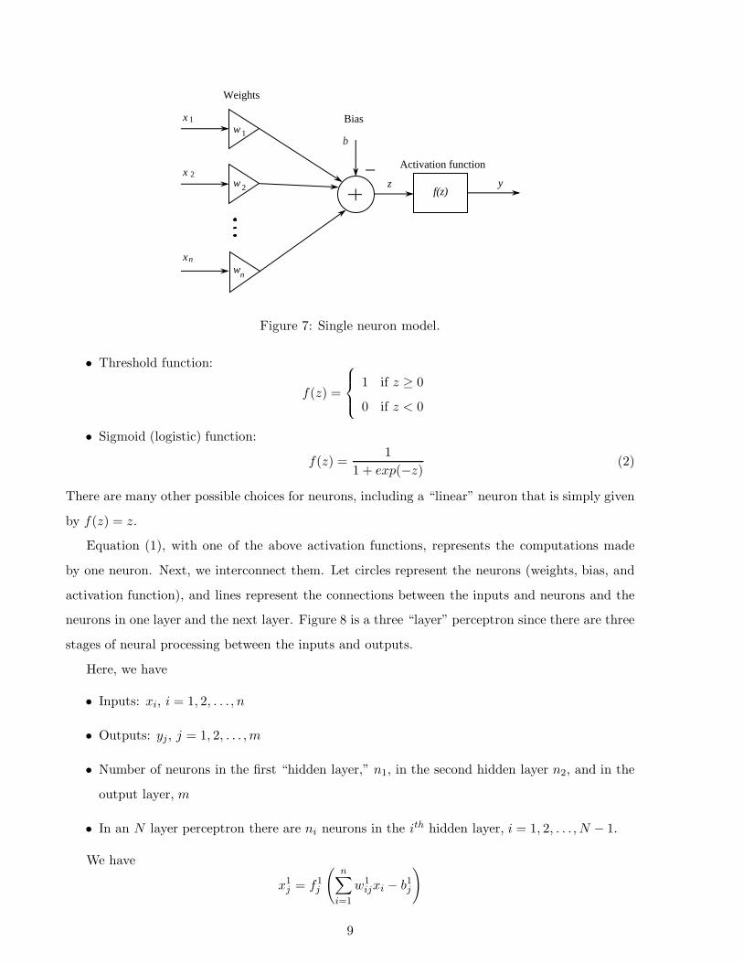
The multilayer perceptron is composed of an interconnected set of neurons, each of which has

the form shown in Figure 7. Here,

z =n∑

i=1

wixi − b

and the wi are the interconnection “weights” and b is the “bias” for the neuron (these parameters

model the interconnections between the cell bodies in the neurons of a biological neural network).

The signal z represents a signal in the biological neuron and the processing that the neuron performs

on this signal is represented with an “activation function” f where

y = f(z) = f

(n∑

i=1

wixi − b

). (1)

The neuron model represents the biological neuron that “fires” (turns on) when its inputs are

significantly excited (i.e., z is big enough). “Firing” is defined by an “activation function” f where

two (of many) possibilities for its definition are:

8

f(z)yz

x

x

x

Activation function

w

w

w

1

1

2

n

2

n

Weights

Bias

b

Figure 7: Single neuron model.

• Threshold function:

f(z) =

1 if z ≥ 00 if z < 0

• Sigmoid (logistic) function:f(z) =

11 + exp(−z)

(2)

There are many other possible choices for neurons, including a “linear” neuron that is simply given

by f(z) = z.

Equation (1), with one of the above activation functions, represents the computations made

by one neuron. Next, we interconnect them. Let circles represent the neurons (weights, bias, and

activation function), and lines represent the connections between the inputs and neurons and the

neurons in one layer and the next layer. Figure 8 is a three “layer” perceptron since there are three

stages of neural processing between the inputs and outputs.

Here, we have

• Inputs: xi, i = 1, 2, . . . , n

• Outputs: yj, j = 1, 2, . . . , m

• Number of neurons in the first “hidden layer,” n1, in the second hidden layer n2, and in the

output layer, m

• In an N layer perceptron there are ni neurons in the ith hidden layer, i = 1, 2, . . . , N − 1.

We have

x1j = f1

j

(n∑

i=1

w1ijxi − b1

j

)

9

(1)

x 1

x 2

xn

.

.

.

x 1

x 2

.

.

.

x 1

x 2

2xn

.

.

.

y

y

y

(1) (2)

m

1

2

(1)

(2)

xn 1(2)

First hiddenlayer

Secondhiddenlayer

Outputlayer

Figure 8: Multilayer perceptron model.

with j = 1, 2, . . . , n1. We have

x2j = f2

j

(n1∑i=1

w2ijx

1i − b2

j

)

with j = 1, 2, . . . , n2. We have

yj = fj

(n2∑i=1

wijx2i − bj

)

with j = 1, 2, . . . , m. Here, we have

• w1ij (w

2ij) are the weights of the first (second) hidden layer

• wij are the weights of the output layer

• b1j are the biases of the first hidden layer.

• b2j are the biases of the second hidden layer

• bj are the biases of the output layer

• fj (for the output layer), f2j (for the second hidden layer), and f1

j (for the first hidden layer)

are the activation functions (all can be different).

10

2.2.2 Training Neural Networks

How do we construct a neural network? We train it with examples. Regardless of the type of

network, we will refer to it as

y = F (x, θ)

where θ is the vector of parameters that we tune to shape the nonlinearity it implements (F could

be a fuzzy system too in the discussion below). For a neural network θ would be a vector of the

weights and biases. Sometimes we will call F an “approximator structure.” Suppose that we gather

input-output training data from a function y = g(x) that we do not have an analytical expression

for (e.g., it could be a physical process).

Suppose that y is a scalar but that x = [x1, . . . , xn]�. Suppose that xi = [xi1, . . . , x

in]

� is the ith

input vector to g and that yi = g(xi). Let the training data set be

G = {(xi, yi) : i = 1, . . . ,M}

The “function approximation problem” is how to tune θ using G so that F matches g(x) at a test

set Γ (Γ is generally a much bigger set than G). For system identification the xi are composed

of past system inputs and outputs (a regressor vector) and the yi are the resulting outputs. In

this case we tune θ so that F implements the system mapping (between regressor vectors and the

output). For parameter estimation the xi can be regressor vectors but the yi are parameters that

you want to estimate. In this way we see that by solving the above function approximation problem

we are able to solve several types of problems in estimation (and control, since estimators are used

in, for example, adaptive controllers).

Consider the simpler situation in which it is desired to cause a neural network F (x, θ) to match

the function g(x) at only a single point x where y = g(x). Given an input x we would like to adjust

θ so that the difference between the desired output and neural network output

e = y − F (x, θ) (3)

is reduced (where y may be either vector or scalar valued). In terms of an optimization problem,

we want to minimize the cost function

J(θ) = e�e. (4)

Taking infinitesimal steps along the gradient of J(θ) with respect to θ will ensure that J(θ) is

nonincreasing. That is, choose

θ = −η � J(θ), (5)

11

where η > 0 is a constant and if θ = [θ1, . . . , θp]�,

�J(θ) =∂J(θ)∂θ

=

∂J(θ)∂θ1

...∂J(θ)∂θp

(6)

Using the definition for J(θ) we get

θ = −η∂e�e∂θ

or

θ = −η∂

∂θ(y − F (x, θ))�(y − F (x, θ))

so that

θ = −η∂

∂θ(y�y − 2F (x, θ)�y + F (x, θ)�F (x, θ))

Now, taking the partial we get

θ = −η(−2∂F (x, θ)�

∂θy + 2

∂F (x, θ)�

∂θF (x, θ))

If we let η = 2η we get

θ = η∂F (x, z)

∂z

∣∣∣∣�

z=θ(y − F (x, θ))

so

θ = ηζ(x, θ)e (7)

where η > 0, and

ζ(x, θ) =∂F (x, z)

∂z

∣∣∣∣�

z=θ, (8)

Using this update method we seek to adjust θ to try to reduce J(θ) so that we achieve good function

approximation.

In discretized form and with non-singleton training sets updating is accomplished by selecting

the pair (xi, yi), where i ∈ {1, . . . ,M} is a random integer chosen at each iteration, and then using

Euler’s first order approximation the parameter update is defined by

θ(k + 1) = θ(k) + ηζi(k)e(k). (9)

where k is the iteration step, e(k) = yi − F (xi, θ(k)) and

ζi(k) =∂F (xi, z)

∂z

∣∣∣∣∣�

z=θ(k)

. (10)

12

When M input-output pairs, or patterns, (xi, yi) where yi = g(xi) are to be matched, “batch

updates” can also be done. In this case, let

ei = yi − F (xi, θ), (11)

and let the cost function be

J(θ) =M∑i=1

ei�ei. (12)

and the update formulas can be derived similarly. This is actually the “backpropagation method”

(except we have not noted the fact that due to the structure of the layered neural networks certain

computational savings are possible). In practical applications the backpropagation method, which

relies on the “steepest descent approach,” can be very slow since the cost J(θ) can have long

low slope regions. It is for this reason that in practice numerical methods are used to update

neural network parameters. Two of the methods that have proven to be particularly useful are the

Levenberg-Marquardt and conjugate-gradient methods. See [12, 13, 4, 16, 8, 5, 32, 17, 21, 14] for

more details.

2.2.3 Design Concerns

There are several design concerns that you encounter in solving the function approximation problem

using gradient methods (or others) to tune the approximator structure. First, it is difficult to

pick a training set G that you know will ensure good approximation (indeed, most often it is

impossible to choose the training set; often some other system chooses it). Second, the choice of

the approximator structure is difficult. While most neural networks (and fuzzy systems) satisfy

the “universal approximation property,” so that they can be tuned to approximate any continuous

function on a closed and bounded set to an arbitrary degree of accuracy, this generally requires

that you be willing to add an arbitrary amount of structure to the approximator (e.g., nodes to a

hidden layer of a multilayer perceptron). Due to finite computing resources we must then accept

an “approximation error.” How do we pick the structure to keep this error as low as possible? This

is an open research problem and algorithms that grow or shrink the structure automatically have

been developed. Third, it is generally impossible to guarantee convergence of the training methods

to a global minimum due to the presence of many local minima. Hence, it is often difficult to know

when to terminate the algorithm (often tests on the size of the gradient update or measures of the

approximation error are used to terminate). Finally, there is the important issue of “generalization,”

where the neural network is hopefully trained to nicely interpolate between similar inputs. It is

very difficult to guarantee that good interpolation is achieved. Normally, all we can do is use a rich

13

data set (large, with some type of uniform and dense spacing of data points) to test that we have

achieved good interpolation. If we have not, then you may not have used enough complexity in

your model structure, or you may have too much complexity that resulted in “over-training” where

you match very well at the training data but there are large excursions elsewhere.

In summary, the main advantage of neural networks is that they can achieve good approximation

accuracy with a reasonable number of parameters by training with data (hence, there is a lack of

dependence on models). We will show how this advantage can be exploited in the next section for

challenging industrial control problems.

2.3 Genetic Algorithms

A genetic algorithm (GA) is a computer program that simulates characteristics of evolution, natural

selection (Darwin), and genetics (Mendel). It is an optimization technique that performs a parallel

(i.e., candidate solutions are distributed over the search space) and stochastic but directed search

to evolve the most fit population. Sometimes when it “gets stuck” at a local optimum it is able to

use the multiple candidate solutions to try to simultaneously find other parts of the search space

that will allow it to “jump out” of the local optimum and find a global one (or at least a better

local one). GAs do not need analytical gradient information, but with modifications can exploit

such information if it is available.

2.3.1 The Population of Individuals

The “fitness function” of a GA measures the quality of the solution to the optimization problem

(in biological terms, the ability of an individual to survive). The GA seeks to maximize the fitness

function J(θ) by selecting the individuals that we represent with the parameters in θ. To represent

the GA in a computer we make θ a string (called a “chromosome”) as shown in Figure 9.

Gene = digit location

Values here = alleles

String of genes = chromosome

Figure 9: String for representing an individual.

In a base-2 representation “alleles” (values in the positions, “genes” on the chromosome) are

0 and 1. In base-10 the alleles take on integer values between 0 and 9. A sample binary chromo-

some is given by: 1011110001010 while a sample base-10 chromosome is: 8219345127066. These

14

chromosomes should not necessarily be interpretted as the corresponding positive integers. We can

add a gene for the sign of the number and fix a position for the decimal point to represent signed

reals. In fact, representation via chromosomes is generally quite abstract. Genes can code for

symbolic or structural characteristics, not just for numeric parameter values, and data structures

for chromosomes can be trees and lattices, not just vectors.

Chromosomes encode the parameters of a fuzzy system, neural network, or an estimator or

controller’s parameters. For example, to tune the fuzzy controller discussed earlier for the tanker

ship you could use the chromosome:

b1b2 · · · b9

(these are the output membership function centers). To tune a neural network you can use a

chromosome that is a concatenation of the weights and biases of the network. Aspects of the

structure of the neural network, such as the number of neurons in a layer, the number of hidden

layers, or the connectivity patterns can also be incorporated into the chromosome. To tune a

proportional-integral-derivative (PID) controller, the chromosome would be a concatenation of its

three gains.

How do we represent a set of individuals (i.e., a population)? Let θji (k) be a single parameter

at time k (a fixed length string with sign digit) and suppose that chromosome j is composed of N

of these parameters that are sometimes called “traits.” Let

θj(k) =[θj1(k), θ

j2(k), . . . , θ

jN(k)

]�.

be the jth chromosome.

The population at time (“generation”) k is

P (k) ={θj(k) : j = 1, 2, . . . , S

}(13)

Normally, you try to pick the population size S to be big enough so that broad exploration of the

search space is achieved, but not too big or you will need too many computational resources to

implement the genetic algorithm.

Evolution occurs as we go from a generation at time k to the next generation at time k+1 via

fitness evaluation, selection, and the use of genetic operators such as crossover and mutation.

15

2.3.2 Genetic Operators

Selection follows Darwin’s theory that the most qualified individuals survive to mate. We quantify

“most qualified” via an individual’s fitness J(θj(k)). We create a “mating pool” at time k:

M(k) ={mj(k) : j = 1, 2, . . . , S

}. (14)

Then, we select an individual for mating by letting each mj(k) be equal to θi(k) ∈ P (k) with

probability

pi =J(θi(k))∑S

j=1 J(θj(k)). (15)

With this approach, more fit individuals will tend to end up mating more often, thereby providing

more off-spring. Less fit individuals, on the other hand, will have contributed less of the genetic

material for the next generation.

Next, in the reproduction phase, that operates on the mating pool, there are two operations:

“crossover” and “mutation.” Crossover is mating in biological terms (the process of combining

chromosomes), for individuals in M(k). For crossover, you first specify the “crossover probability”

pc (usually chosen to be near unity). The procedure for crossover is: Randomly pair off the

individuals in the mating poolM(k). Consider chromosome pair θj , θi. Generate a random number

r ∈ [0, 1]. If r ≥ pc then do not crossover (just pass the individuals into the next generation). If

r < pc then crossover θj and θi. To crossover these chromosomes select at random a “cross site”

and exchange all the digits to the right of the cross site of one string with the other (see Figure 10).

Note that multi-point (multiple cross sites) crossover operators can also be used, with the offspring

chromosomes composed by alternating chromosome segments from the parents.

θ i 1 2 3 4 5 6 7 8 9 10 11 12 13

θ j 1 2 3 4 5 6 7 8 9 10 11 12 13

Cross site

Switch these two parts of the strings

Figure 10: Crossover operation example.

Crossover perturbs the parameters near good positions to try to find better solutions to the

optimization problem. It tends to perform a localized search around the more fit individuals (i.e.,

children are interpolations of their parents that may be more or less fit to survive).

16

Next, in the reproduction phase, after crossover, we have mutation. The biological analog of

our mutation operation is the random mutation of genetic material. To do this, with probability

pm change (mutate) each gene location on each chromosome (in the mating pool) randomly to a

member of the number system being used. Mutation tries to make sure that we do not get stuck

at a local maximum of the fitness function and that we seek to explore other areas of the search

space to help find a global maximum for J(θ). Since mutation is pure random search, pm is usually

near zero.

Finally, we produce the next generation by letting

P (k + 1) =M(k)

Evolution is the repetition of the above process. For more details on GAs see [22, 20, 28, 10].

2.3.3 Design Concerns

There are many design concerns that one can encounter when using GAs to solve optimization

problems. First, it is important to fully understand the optimization problem, know what you

want to optimize, and what you can change to achieve the optimization. You also must have an

idea of what you will accept as an optimal solution. Second, choice of representation (e.g., the

number of digits in a base-10 representation) is important. Too detailed of a representation causes

increases in computational complexity while if the representation is too coarse then you may not

be able to achieve enough accuracy in your solution. Third, there are a wide range of other genetic

operators (e.g., “elitism” where the most fit individual is passed to the next generation without

being perturbed by crossover or mutation) and choosing the appropriate ones is important since

they can affect convergence significantly. Fourth, just like for gradient optimization methods it is

important to pick a good termination method (even if it is simply a test on how much improvement

has been made on J over the last several generations). Finally, for practical problems it is difficult

to guarantee that you will achieve convergence due to the presence of local maxima. Moreover, it

can be difficult to select the best solution from the many candidate solutions that exist (most often

you pick the parameters that resulted in the highest value of the fitness function and these may

have been generated in a past generation, not at the final one).

In summary, the main advantage of genetic algorithms is that they offer an evolution-based

stochastic search that can be useful in finding good solutions to practical complex optimization

problems, especially when gradient information is not conveniently available.

17

2.4 Expert and Planning Systems

In this section we briefly overview the expert and planning systems [27] approaches to control. We

keep the discussion particularly brief since the use of expert systems for control (“expert control”)

is conceptually similar to fuzzy control and since general planning operations often fall outside the

area of traditional control problems (although they probably should not).

2.4.1 Expert Control

For the sake of our discussion, we will simply view the expert system that is used here as a controller

for a dynamic system, as is shown in Figure 11. Here, we have an expert system serving as feedback

controller with reference input r and feedback variable y. It uses the information in its knowledge-

base and its inference mechanism to decide what command input u to generate for the plant.

Conceptually, we see that the expert controller is closely related to the fuzzy controller. There are,

however, several differences. First, the knowledge-base in the expert controller could be a rule-base,

but is not necessarily so. It could be developed using other knowledge-representation structures,

such as frames, semantic nets, causal diagrams, and so on. Second, the inference mechanism in the

expert controller is more general than that of the fuzzy controller. It can use more sophisticated

matching strategies to determine which rules should be allowed to fire. It can use more elaborate

inference strategies such as “refraction,” “recency,” and various other priority schemes. Next, we

should note that Figure 11 shows a direct expert controller. It is also possible to use an expert

system as a supervisor for conventional or intelligent controllers.

Fuzz

ific

atio

n

Def

uzzi

fica

tion

FuzzyInferenceMechanis

m

Rule-BaseKnowledge-base

Process

Inputs OutputsReference input

Expert controller

r(t) u(t) y(t)

Inferencemechanism

Figure 11: Expert control system.

2.4.2 Planning Systems for Control

Artificially intelligent planning systems (computer programs that are often designed to emulate

the way experts plan) have been used for several problems, including path planning and high-level

18

decisions about control tasks for robots [6, 27]. A generic planning system can be configured in the

architecture of a standard control system, as shown in Figure 12. Here, the “problem domain” (the

plant) is the environment that the planner operates in. There are measured outputs yk at step k

(variables of the problem domain that can be sensed in real time), control actions uk (the ways in

which we can affect the problem domain), disturbances dk (which represent random events that can

affect the problem domain and hence the measured variable yk), and goals gk (what we would like

to achieve in the problem domain). There are closed-loop specifications that quantify performance

and stability requirements. It is the task of the planner in Figure 12 to monitor the measured

outputs and goals and generate control actions that will counteract the effects of the disturbances

and result in the goals and the closed-loop specifications being achieved. To do this, the planner

performs “plan generation,” where it projects into the future (usually a finite number of steps, and

often using a model of the problem domain) and tries to determine a set of candidate plans. Next,

this set of plans is pruned to one plan that is the best one to apply at the current time (where

“best” can be determined based on, e.g., consumption of resources). The plan is then executed,

and during execution the performance resulting from the plan is monitored and evaluated. Often,

due to disturbances, plans will fail, and hence the planner must generate a new set of candidate

plans, select one, then execute that one. While not pictured in Figure 12, some planning systems

use “situation assessment” to try to estimate the state of the problem domain (this can be useful in

execution monitoring and plan generation); others perform “world modeling,” where a model of the

problem domain is developed in an on-line fashion (similarly to on-line system identification), and

“planner design” uses information from the world modeler to tune the planner (so that it makes

the right plans for the current problem domain). The reader will, perhaps, think of such a planning

system as a general adaptive (model predictive) controller.

Planstep

Findproblem

Plan generation

Project(Re )Plan

Setof

plansOneplan

Planner

Plandecisions

Planexecution

Goals

Problemdomain

Controlactions

Measuredoutputs

Disturbances dk

uk

yk

gk

Execution monitoringPlanfailure

Figure 12: Closed-loop planning system.

19

2.5 Intelligent and Autonomous Control

Autonomous systems have the capability to independently (and successfully) perform complex

tasks. Consumer and governmental demands for such systems are frequently forcing engineers to

push many functions normally performed by humans into machines. For instance, in the emerg-

ing area of intelligent vehicle and highway systems (IVHS), engineers are designing vehicles and

highways that can fully automate vehicle route selection, steering, braking, and throttle control to

reduce congestion and improve safety. In avionic systems a “pilot’s associate” computer program

has been designed to emulate the functions of mission and tactical planning that in the past may

have been performed by the copilot. In manufacturing systems, efficiency optimization and flow

control are being automated, and robots are replacing humans in performing relatively complex

tasks. From a broad historical perspective, each of these applications began at a low level of au-

tomation, and through the years each has evolved into a more autonomous system. For example,

automotive cruise controllers are the ancestors of the (research prototype) controllers that achieve

coordinated control of steering, braking, and throttle for autonomous vehicle driving. And the

terrain following and terrain avoidance control systems for low-altitude flight are ancestors of an

artificial pilot’s associate that can integrate mission and tactical planning activities. The general

trend has been for engineers to incrementally “add more intelligence” in response to consumer,

industrial, and government demands and thereby create systems with increased levels of autonomy.

In this process of enhancing autonomy by adding intelligence, engineers often study how humans

solve problems, then try to directly automate their knowledge and techniques to achieve high levels

of automation. Other times, engineers study how intelligent biological systems perform complex

tasks, then seek to automate “nature’s approach” in a computer algorithm or circuit implementa-

tion to solve a practical technological problem (e.g., in certain vision systems). Such approaches

where we seek to emulate the functionality of an intelligent biological system (e.g., the human)

to solve a technological problem can be collectively named “intelligent systems and control tech-

niques.” It is by using such techniques that some engineers are trying to create highly autonomous

systems such as those listed above.

Figure 13 shows a functional architecture for an intelligent autonomous controller with an in-

terface to the process involving sensing (e.g., via conventional sensing technology, vision, touch,

smell, etc.), actuation (e.g., via hydraulics, robotics, motors, etc.), and an interface to humans

(e.g., a driver, pilot, crew, etc.) and other systems. The “execution level” has low-level numeric

signal processing and control algorithms (e.g., PID, optimal, adaptive, or intelligent control; param-

20

eter estimators, failure detection and identification (FDI) algorithms). The “coordination level”

provides for tuning, scheduling, supervision, and redesign of the execution-level algorithms, crisis

management, planning and learning capabilities for the coordination of execution-level tasks, and

higher-level symbolic decision making for FDI and control algorithm management. The “manage-

ment level” provides for the supervision of lower-level functions and for managing the interface to

the human(s) and other systems. In particular, the management level will interact with the users

in generating goals for the controller and in assessing the capabilities of the system. The man-

agement level also monitors performance of the lower-level systems, plans activities at the highest

level (and in cooperation with humans), and performs high-level learning about the user and the

lower-level algorithms. Conventional or intelligent systems methods can be used at each level. For

more information on these types of control systems see [2, 29, 1, 30, 11].

Humans and other subsystems

Process

Management level

Coordinationlevel

Executionlevel

Figure 13: Intelligent autonomous controller.

3 Applications

In this section some of the main characteristics of the intelligent system methods that have proven

useful in industrial applications are outlined. Then, examples are given for use of the methods.

3.1 Heuristic Construction of Nonlinear Controllers

The first area we discuss where intelligent control has had a clear impact in industry is the area

of heuristic construction of nonlinear controllers. Two areas in intelligent control have made most

21

of the contributions to this area: fuzzy control and expert systems for control (here we will focus

on fuzzy control, one type of rule-based controller, since the ideas extend directly to the expert

control case). The reason that the methods are “heuristic” is that they normally do not rely on

the development and use of a mathematical model of the process to be controlled.

3.1.1 Model-Free Control?

To begin with it is important to critically examine the claim that fuzzy control is “model-free”

control. So, is a model used in the fuzzy control design methodology? It is possible that a math-

ematical model is not used and that the entire process simply relies on the ad hoc specification

of rules about how to control a process (in an analogous manner to how PID controllers are often

designed and implemented in industry). However, often a model is used in simulation to redesign

a fuzzy controller (consider the earlier ship steering controller design problem). Others argue that

a model is always used: even if it is not written down, some type of model is used “in your head”

(even though it might not be a formal mathematical model).

Since most people claim that no formal model is used in the fuzzy control design methodology,

the following questions arise:

1. Is it not true that there are few, if any, assumptions to be violated by fuzzy control and that

the technique can be indiscriminately applied? Yes, and sometimes it is applied to systems

where it is clear that a PID controller or look-up table would be just as effective. So, if this is

the case, then why not use fuzzy control? Because it is more computationally complex than

a PID controller and the PID controller is much more widely understood.

2. Are heuristics all that are available to perform fuzzy controller design? No. Any good models

that can be used, probably should be.

3. By ignoring a formal model, if it is available, is it not the case that a significant amount

of information about how to control the plant is ignored? Yes. If, for example, you have a

model of a complex process, we often use simulations to gain an understanding of how best

to control the plant—and this knowledge can be used to design a fuzzy controller.

Regardless, there are times when it is either difficult or virtually impossible to develop a useful

mathematical model. In such instances, heuristic constructive methods for controllers can be very

useful (of course we often do the same thing with PID controllers).

In the next section we give an example where fuzzy controllers were developed and proved to

be very effective, and no mathematical model was used.

22

3.1.2 Example: Vibration Damping in a Flexible-Link Robot

For nearly a decade, control engineers and roboticists alike have been investigating the problem of

controlling robotic mechanisms that have very flexible links. Such mechanisms are important in

space structure applications, where large, lightweight robots are to be utilized in a variety of tasks,

including deployment, spacecraft servicing, space-station maintenance, and so on. Flexibility is not

designed into the mechanism; it is usually an undesirable characteristic that results from trading off

mass and length requirements in optimizing effectiveness and “deployability” of the robot. These

requirements and limitations of mass and rigidity give rise to many interesting issues from a control

perspective. Why turn to fuzzy control for this application?

The modeling complexity of multilink flexible robots is well documented, and numerous re-

searchers have investigated a variety of techniques for representing flexible and rigid dynamics of

such mechanisms. Equally numerous are the works addressing the control problem in simulation

studies based on mathematical models, under assumptions of perfect modeling. Even in simulation,

however, a challenging control problem exists; it is well known that vibration suppression in slew-

ing mechanical structures whose parameters depend on the configuration (i.e., are time varying)

can be extremely difficult to achieve. Compounding the problem, numerous experimental studies

have shown that when implementation issues are taken into consideration, modeling uncertainties

either render the simulation-based control designs useless, or demand extensive tuning of controller

parameters (often in an ad hoc manner).

Hence, even if a relatively accurate model of the flexible robot can be developed, it is often

too complex to use in controller development, especially for many control design procedures that

require restrictive assumptions for the plant (e.g., linearity). It is for this reason that conventional

controllers for flexible robots are developed either (1) via simple crude models of the plant behavior

that satisfy the necessary assumptions (e.g., either from first principles or using system identification

methods), or (2) via the ad hoc tuning of linear or nonlinear controllers. Regardless, heuristics enter

the design process when the conventional control design process is used.

It is important to emphasize, however, that such conventional control-engineering approaches

that use appropriate heuristics to tune the design have been relatively successful. For a process

such as a flexible robot, you are left with the following question: How much of the success can be

attributed to the use of the mathematical model and conventional control design approach, and

how much should be attributed to the clever heuristic tuning that the control engineer uses upon

implementation? Why not simply acknowledge that much of the problem must be solved with

23

heuristic ideas and avoid all the work that is needed to develop the mathematical models? Fuzzy

control provides such an opportunity and has in fact been shown to be quite successful for this

application [23] compared to conventional control approaches, especially if one takes into account

the efforts needed to develop a mathematical model that is needed for the conventional approaches.

3.2 Data-Based Nonlinear Estimation

The second major area where methods from intelligent control have had an impact in industry is in

the use of neural networks to construct mappings from data. In particular, neural network methods

have been found to be quite useful in pattern recognition and estimation. Below, we explain how

to construct neural network based estimators and give an example where such a method was used.

3.2.1 Estimator Construction Methodology

In conventional system identification you gather plant input-output data and construct a model

(mapping) between the inputs and outputs. In this case, model construction is often done by

tuning the parameters of a model (e.g., the parameters of a linear mapping can be tuned using

linear least squares methods or gradient methods). To validate this model you gather novel plant

input-output data and pass the inputs into your constructed model and compare its outputs to the

ones that were generated by the model. If some measure of the difference between the plant and

model outputs is small, then we accept that the model is a good representation of the system.

Neural networks or fuzzy systems are also tunable functions that could be used for this system

identification task. Fuzzy and neural systems are nonlinear and are parameterized by membership

function parameters or weights (and biases), respectively. Gradient methods can be used to tune

them to match mappings that are characterized with data. Validation of the models proceeds along

the same lines as with conventional system identification.

In certain situations you can also gather data that relates the inputs and outputs of the system

to parameters within the system. To do this, you must be able to vary system parameters and

gather data for each value of the system parameter (the gathered data should change each time

the parameter changes and it is either gathered via a sophisticated simulation model or via actual

experiments with the plant). Then, using a gradient method you can adjust the neural or fuzzy

system parameters to minimize the estimation error. The resulting system can serve as a parameter

estimator (i.e., after it is tuned–normally it cannot be tuned on-line because actual values of the

parameters are not known on-line, they are what you are trying to estimate).

24

3.2.2 Example: Automotive Engine Failure Estimation

In recent years significant attention has been given to reducing exhaust gas emissions produced

by internal combustion engines. In addition to overall engine and emission system design, correct

or fault-free engine operation is a major factor determining the amount of exhaust gas emissions

produced in internal combustion engines. Hence, there has been a recent focus on the development

of on-board diagnostic systems that monitor relative engine health. Although on-board vehicle

diagnostics can often detect and isolate some major engine faults, due to widely varying driving

environments they may be unable to detect minor faults, which may nonetheless affect engine

performance. Minor engine faults warrant special attention because they do not noticeably hinder

engine performance but may increase exhaust gas emissions for a long period of time without the

problem being corrected. The minor faults we consider in this case study include “calibration

faults” (here, the occurrence of a calibration fault means that a sensed or commanded signal is

multiplied by a gain factor not equal to one, while in the no-fault case the sensed or commanded

signal is multiplied by one) in the throttle and mass fuel actuators, and in the engine speed and

mass air sensors. The reliability of these actuators and sensors is particularly important to the

engine controller since their failure can affect the performance of the emissions control system.

Here, we simply discuss how to formulate the problem so that it can be solved with neural or fuzzy

estimation schemes. The key to this is to understand how data is generated for the training of

neural or fuzzy system estimators.

The experimental setup in the engine test cell consists of a Ford 3.0 L V-6 engine coupled to

an electric dynamometer through an automatic transmission. An air charge temperature sensor

(ACT), a throttle position sensor (TPS), and a mass airflow sensor (MAF) are installed in the engine

to measure the air charge temperature, throttle position, and air mass flow rate. Two heated

exhaust gas oxygen sensors (HEGO) are located in the exhaust pipes upstream of the catalytic

converter. The resultant airflow information and input from the various engine sensors are used

to compute the required fuel flow rate necessary to maintain a prescribed air-to-fuel ratio for the

given engine operation. The central processing unit (EEC-IV) determines the needed injector pulse

width and spark timing, and outputs a command to the injector to meter the exact quantity of fuel.

An ECM (electronic control module) breakout box is used to provide external connections to the

EEC-IV controller and the data acquisition system. The angular velocity sensor system consists of

a digital magnetic zero-speed sensor and a specially designed frequency-to-voltage converter, which

converts frequency signals proportional to the rotational speed into an analog voltage.

25

Data is sampled every engine revolution. A variable load is produced through the dynamome-

ter, which is controlled by a DYN-LOC IV speed/torque controller in conjunction with a DTC-1

throttle controller installed by DyneSystems Company. The load torque and dynamometer speed

are obtained through a load cell and a tachometer, respectively. The throttle and the dynamometer

load reference inputs are generated through a computer program and sent through an RS-232 serial

communication line to the controller. Physical quantities of interest are digitized and acquired uti-

lizing a National Instruments AT-MIO-16F-5 A/D timing board for a personal computer. Due to

government mandates, periodic inspections and maintenance for engines are becoming more com-

mon. One such test developed by the Environmental Protection Agency (EPA) is the Inspection

and Maintenance (IM) 240 cycle. The EPA IM240 cycle represents a driving scenario developed

for the purpose of testing compliance of vehicle emissions systems for contents of carbon monoxide

(CO), unburned hydrocarbons (HC), and nitrogen oxides (NOx). A modified version of this cycle

was used in all the tests.

Using the engine test cell, measurements are taken of engine inputs and outputs for various

calibration faults (i.e., we gather sequences of data for each fault). Then, we induce faults over the

whole range of possible values of calibration faults. Data from all these experiments becomes our

training data set (the set G described in the neural network section). This allows us to construct

neural or fuzzy estimators for calibration faults that can be tested in the actual experimental

testbed. Additional details on this application are given in [18].

3.3 Intelligent Adaptive Control Strategies

In this section we overview how intelligent systems methods can be used to achieve adaptive control.

Rather than providing a detailed overview of all the (many) strategies that have been investigated

and reported in the literature, an overview will be provided in the first subsection of this section

that will show how all the methods broadly relate to each other. The reader should keep in mind

that all of these methods bear very close relationships to the work in conventional adaptive control

[15].

3.3.1 Fuzzy, Neural, and Genetic Adaptive Control

There are two general approaches to adaptive control, and in the first one, which is depicted in

Figure 14, we use an on-line system identification method to estimate the parameters of the plant

(by estimating the parameters of an “identifier model”) and a “controller designer” module to

subsequently specify the parameters of the controller. If the plant parameters change, the identifier

26

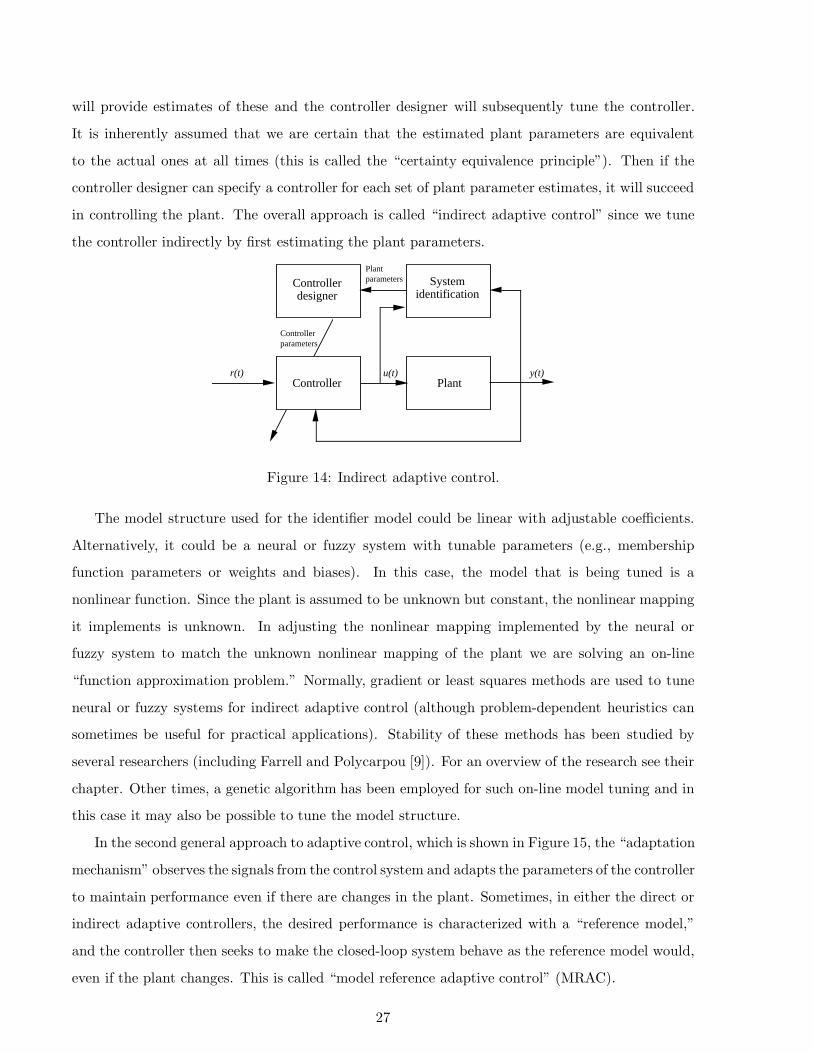
will provide estimates of these and the controller designer will subsequently tune the controller.

It is inherently assumed that we are certain that the estimated plant parameters are equivalent

to the actual ones at all times (this is called the “certainty equivalence principle”). Then if the

controller designer can specify a controller for each set of plant parameter estimates, it will succeed

in controlling the plant. The overall approach is called “indirect adaptive control” since we tune

the controller indirectly by first estimating the plant parameters.

PlantController

Systemidentification

Controllerdesigner

r(t) u(t) y(t)

Plantparameters

Controllerparameters

Figure 14: Indirect adaptive control.

The model structure used for the identifier model could be linear with adjustable coefficients.

Alternatively, it could be a neural or fuzzy system with tunable parameters (e.g., membership

function parameters or weights and biases). In this case, the model that is being tuned is a

nonlinear function. Since the plant is assumed to be unknown but constant, the nonlinear mapping

it implements is unknown. In adjusting the nonlinear mapping implemented by the neural or

fuzzy system to match the unknown nonlinear mapping of the plant we are solving an on-line

“function approximation problem.” Normally, gradient or least squares methods are used to tune

neural or fuzzy systems for indirect adaptive control (although problem-dependent heuristics can

sometimes be useful for practical applications). Stability of these methods has been studied by

several researchers (including Farrell and Polycarpou [9]). For an overview of the research see their

chapter. Other times, a genetic algorithm has been employed for such on-line model tuning and in

this case it may also be possible to tune the model structure.

In the second general approach to adaptive control, which is shown in Figure 15, the “adaptation

mechanism” observes the signals from the control system and adapts the parameters of the controller

to maintain performance even if there are changes in the plant. Sometimes, in either the direct or

indirect adaptive controllers, the desired performance is characterized with a “reference model,”

and the controller then seeks to make the closed-loop system behave as the reference model would,

even if the plant changes. This is called “model reference adaptive control” (MRAC).

27

PlantController

Adaptationmechanism

r(t) u(t) y(t)

Figure 15: Direct adaptive control.

In neural control or adaptive fuzzy control the controller is implemented with a neural or fuzzy

system, respectively. Normally, gradient or least squares methods are used to tune the controller

(although sometimes problem-dependent heuristics have been found to be quite useful for practical

applications, such as in the fuzzy model reference learning controller discussed below). Stability

of direct adaptive neural or fuzzy methods has been studied by several researchers (again, for an

overview of the research see the chapter by Farrell and Polycarpou [9]). Clearly, since the genetic

algorithm is also an optimization method, it can be used to tune neural or fuzzy system mappings

when they are used as controllers also. The key to making such a controller work is to provide a way

to define a fitness function for evaluating the quality of a population of controllers (in one approach

a model of the plant is used to predict into the future how each controller in the population will

perform). Then, the most fit controller in the population is used at each step to control the plant.

This is a type of adaptive model predictive control (MPC) method.

Finally, we would like to note that in practical applications it is sometimes found that a “su-

pervisory controller” can be very useful. Such a controller takes as inputs data from the plant and

the reference input (and any other information available, e.g., from the user) and tunes the under-

lying control strategy. For example, for the flexible-link robot application discussed earlier such

a strategy was found to be very useful in tuning a fuzzy controller and in an aircraft application

it was found useful in tuning an adaptive fuzzy controller to try to ensure that the controller was

maximally sensitive to plant failures in the sense that it would quickly respond to them, but still

maintained stable high performance operation.

3.3.2 Example: Adaptive Fuzzy Control for Ship Steering

How good is the fuzzy controller that we designed for the ship steering problem earlier in this

chapter? Between trips, let there be a change from “ballast” to “full” conditions on the ship (a

28

weight change). In this case, using the controller we had developed earlier, we get the response in

Figure 16.

0 500 1000 1500 2000 2500 3000 3500 4000-10

0

10

20

30

40

50

60

Time (sec)

Ship heading (solid) and desired ship heading (dashed), deg.

0 500 1000 1500 2000 2500 3000 3500 4000-60

-40

-20

0

20

40

60

80

Time (sec)

Rudder angle (δ), deg.

Figure 16: Response of fuzzy control system for tanker heading regulation, weight change.

Clearly there has been a significant degradation in performance. It is possible to tune the fuzzy

controller to reduce the effect of this disturbance, but there can then be other disturbances that

could also have adverse effects on performance. This presents a fundamental challenge to fuzzy

control and motivates the need for a method that can automatically tune the fuzzy controller if

there are changes in the plant.

Fuzzy model reference learning control (FMRLC) is one heuristic approach to adaptive fuzzy

control and the overall scheme is shown in Figure 17. Here, at the lower level in the figure there is a

plant that is controlled by a fuzzy controller (as an example, this one simply has inputs of the error

and change in error). The “reference model” is a user-specified dynamical system that is used to

quantify how we would like the system to behave between the reference input and the plant output.

For example, we may request a first order response with a specified time constant between the

reference input and plant output. The “learning mechanism” observes the performance of the low-

level fuzzy controller loop and decides when to update the fuzzy controller. For this example, when

the error between the reference model output and the plant output is large the learning mechanism

will make large changes to the fuzzy controller (by tuning its output membership function centers),

29

while if this error is small, then it will make small changes. For more details, see [19].

Planty(kT)

1-z -1

T

1-z-1

T

Knowledge-base

gc

ge

Inferencemechanism

Fuzzy sets Rule-base

Σ

Σ

Fuzzy controller

gue(kT)

u(kT)

r (kT)

ye(kT)

+

yc(kT)

+

gyc

gye

gp

Inferencemechanism

Knowledge-base

Referencemodel

p(kT)

Storage

Knowledge-basemodifier

Fuzzy inverse model

my (kT)

Learning mechanism

Figure 17: Fuzzy model reference learning controller.

How does the FMRLC work for the tanker ship? Assume that we initialize the controller with

the one that was developed via manual tuning earlier. To see that it can tune a rule-base see the

response in Figure 18 (we use a first order reference model). Here, at t = 9000 sec. the ship weight is

suddenly changed from ballast to full and we see that while initially the weight change causes poor

transient performance, it quickly recovers to provide good tracking. Compare this response to the

direct fuzzy controller results in Figure 16. You can see that it does very well at tuning the fuzzy

controller (although it may not be done tuning at the end of the simulation). The tuned controller

surface (at the end of the simulation) is shown in Figure 19 and we see that it produced some shape

changes relative to the manually constructed one in Figure 6 since it is trying to compensate for

the effects of the weight change.

4 Concluding Remarks: Outlook on Intelligent Control

In this section we briefly note some of the current and future research directions in intelligent

control. Current theoretical research in intelligent control is focusing on:

• Mathematical stability/convergence/robustness analysis for learning systems.

• Mathematical comparative analysis with nonlinear adaptive methods.

30

0 0.2 0.4 0.6 0.8 1 1.2 1.4 1.6 1.8 2

x 104

-20

0

20

40

60Ship heading (solid) and desired ship heading (dashed), deg.

0 0.2 0.4 0.6 0.8 1 1.2 1.4 1.6 1.8 2

x 104

-100

-50

0

50

100Rudder angle, output of fuzzy controller (input to the ship), deg.

0 0.2 0.4 0.6 0.8 1 1.2 1.4 1.6 1.8 2

x 104

-0.1

-0.05

0

0.05

0.1

Time (sec)

Fuzzy inverse model output (nonzero values indicate adaptation)

Figure 18: FMRLC response, rule-base tuning for tanker.

-150-100

-500

50100

150

-0.4

-0.2

0

0.2

0.4

-100

-50

0

50

100

Heading error (e), deg.

FMRLC-tuned fuzzy controller mapping between inputs and output

Change in heading error (c), deg.

Fuz

zy c

ontr

olle

r ou

tput

(δ)

, deg

.

Figure 19: FMRLC response, rule-base tuning for tanker, tuned controller surface.

However, as Albert Einstein once said: “So far as the laws of mathematics refer to reality, they

are not certain. And so far as they are certain, they do not refer to reality.” Or stated another

31

way, your approaches that are developed with mathematical analysis are only as good as the model

that you use to develop them.

Current research on the development of new techniques in intelligent control focuses on the

following:

• Complex heuristic learning strategies.

• Memory and computational savings.

• Coping with “hybrid” discrete event / differential equation models.

Current research in applications and implementations is focusing on a wide variety of problems.

It is important to note the following:

• There is a definite need for experimental research (especially in comparative analysis and newnon-traditional applications).

• There have been definite successes in industry (we are certainly not providing a completeoverview of these successess).

• For researchers in universities, working with industry is challenging and important.

In summary, intelligent control not only tries to borrow ideas from the sciences of physics and

mathematics to help develop control systems, but also biology, neuroscience, artificial intelligence,

and others. It has proven useful in some applications as we discussed in the previous section, and

may offer useful solutions to the challenging problems that you encounter.

Acknowledgements: The author would like to thank J. Spooner who had worked with the author

on writing an earlier version of Section 2.2.2. Also, the author would like to thank the editor T.

Samad for his helpful edits and for organizing the writing of this book.

References

[1] J. S. Albus. Outline for a theory of intelligence. IEEE Trans. on Systems, Man, and Cyber-

netics, 21(3):473–509, May/Jun. 1991.

[2] P. J. Antsaklis and K. M. Passino, editors. An Introduction to Intelligent and Autonomous

Control. Kluwer Academic Publishers, Norwell, MA, 1993.

32

[3] K. J. Astrom and B. Wittenmark. Adaptive Control. Addison-Wesley, Reading, MA, 1995.

[4] D. P. Bertsekas. Nonlinear Programming. Athena Scientific Press, Belmont, MA, 1995.

[5] M. Brown and C. Harris. Neurofuzzy Adaptive Modeling and Control. Prentice-Hall, Englewood

Cliffs, NJ, 1994.

[6] T. Dean and M. P. Wellman. Planning and Control. Morgan Kaufman, San Mateo, CA, 1991.

[7] D. Driankov, H. Hellendoorn, and M. Reinfrank. An Introduction to Fuzzy Control. Springer-

Verlag, New York, 1993.

[8] J. Farrell. Neural control. In W. Levine, editor, The Control Handbook, pages 1017–1030. CRC

Press, Boca Raton, FL, 1996.

[9] J. Farrell and M. Polycarpou. On-line approximation based control with neural networks and

fuzzy systems. In T. Samad, editor, Perspectives in Control: New Concepts and Applications,

page ?? IEEE Press, Piscataway, NJ, 1999.

[10] D. Goldberg. Genetic Algorithms in Search, Optimization and Machine Learning. Addison-

Wesley, Reading, MA, 1989.

[11] M. Gupta and N. Sinha, editors. Intelligent Control: Theory and Practice. IEEE Press,

Piscataway, NJ, 1995.

[12] M. Hagan, H. Demuth, and M. Beale. Neural Network Design. PWS Publishing, Boston, MA,

1996.

[13] J. Hertz, A. Krogh, and R. G. Palmer. Introduction to the Theory of Neural Computation.

Addison-Wesley, Reading, MA, 1991.

[14] K. J. Hunt, D. Sbarbaro, R. Zbikowski, and P. J. Gawthrop. Neural networks for control

systems: A survey. In M. M. Gupta and D. H. Rao, editors, Neuro-Control Systems: Theory

and Applications, pages 171–200. IEEE Press, Piscataway, NJ, 1994.

[15] P. A. Ioannou and J. Sun. Robust Adaptive Control. Prentice-Hall, Englewood Cliffs, NJ, 1996.

[16] J.-S. R. Jang, C.-T. Sun, and E. Mizutani. Neuro-Fuzzy and Soft Computing: A Computational

Approach to Learning and Machine Intelligence. Prentice Hall, NJ, 1997.

[17] B. Kosko. Neural Networks and Fuzzy Systems. Prentice-Hall, Englewood Cliffs, NJ, 1992.

33

[18] E. G. Laukonen, K. M. Passino, V. Krishnaswami, G.-C. Luh, and G. Rizzoni. Fault detection

and isolation for an experimental internal combustion engine via fuzzy identification. IEEE

Trans. on Control Systems Technology, 3(3):347–355, September 1995.

[19] J. R. Layne and K. M. Passino. Fuzzy model reference learning control for cargo ship steering.

IEEE Control Systems Magazine, 13(6):23–34, December 1993.

[20] Z. Michalewicz. Genetic Algorithms + Data Structure = Evolution Programs. Springer-Verlag,

Berlin, 1992.

[21] W. T. Miller, R. S. Sutton, and P. J. Werbos, editors. Neural Networks for Control. The MIT

Press, Cambridge, MA, 1991.

[22] M. Mitchell. An Introduction to Genetic Algorithms. MIT Press, Cambridge, MA, 1996.

[23] V. G. Moudgal, K. M. Passino, and S. Yurkovich. Rule-based control for a flexible-link robot.

IEEE Trans. on Control Systems Technology, 2(4):392–405, December 1994.

[24] R. Palm, D. Driankov, and H. Hellendoorn. Model Based Fuzzy Control. Springer-Verlag, New

York, 1997.

[25] Kevin M. Passino and Stephen Yurkovich. Fuzzy Control. Addison Wesley Longman, Menlo

Park, CA, 1998.

[26] T. Ross. Fuzzy Logic in Engineering Applications. McGraw-Hill, New York, 1995.

[27] S. Russell and P. Norvig. Artificial Intelligence: A Modern Approach. Prentice Hall, NJ, 1995.

[28] M. Srinivas and L. M. Patnaik. Genetic algorithms: A survey. IEEE Computer Magazine,

pages 17–26, June 1994.

[29] R. F. Stengel. Toward intelligent flight control. IEEE Trans. on Systems, Man, and Cyber-

netics, 23(6):1699–1717, Nov./Dec. 1993.

[30] K. Valavanis and G. Saridis. Intelligent Robotic Systems: Theory, Design, and Applications.

Kluwer Academic Publishers, Norwell, MA, 1992.

[31] L.-X. Wang. A Course in Fuzzy Systems and Control. Prentice-Hall, Englewood Cliffs, NJ,

1997.

[32] D. White and D. Sofge, editors. Handbook of Intelligent Control: Neural, Fuzzy and Adaptive

Approaches. Van Nostrand Reinhold, New York, 1992.

34