Integration of dynamic land use change into SWAT using the LUP.dat file

and an advanced setup tool

Introduction

Conclusions

& Prospects

LUPSA

Test Case &

LUPSA app.

SWAT & LUC

Input Type

Scale Geological Centuries Decades Years Days Hours

Terrain

Soil

Land UseSWAT Input

Climate

Static Dynamic

Dynamics of SWAT Input

SWAT Input

Introduction

Conclusions

& Prospects

LUPSA

Test Case &

LUPSA app.

SWAT & LUC

Actual

Cropland

in Eastern

Europe

Introduction

Conclusions

& Prospects

LUPSA

Test Case &

LUPSA app.

SWAT & LUC

Abandonment

of cropland

in Eastern

Europe

Introduction

Conclusions

& Prospects

LUPSA

Test Case &

LUPSA app.

SWAT & LUC

Input Type

Land Use

Scale Geological Centuries Decades Years Days Hours

Terrain

SoilSWAT Input

Climate

Static Dynamic

Dynamics of SWAT Input

• Impact on Calibration/Validation once a model is

calibrated for several years?

• Impact on projections? What if I want information on a

shifting process projected by a single future scenario

• What if I would like to use the model for scenario

optimization effected by land use dynamics? (e.g. using

a Pareto optimum)

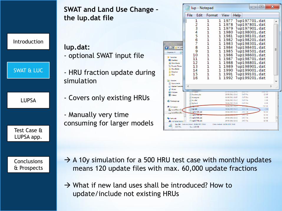
SWAT and Land Use Change –

the lup.dat file

lup.dat:

- optional SWAT input file

- HRU fraction update during

simulation

- Covers only existing HRUs

- Manually very time

consuming for larger models

A 10y simulation for a 500 HRU test case with monthly updates

means 120 update files with max. 60,000 update fractions

What if new land uses shall be introduced? How to

update/include not existing HRUs

Conclusions

& Prospects

LUPSA

Test Case &

LUPSA app.

SWAT & LUC

Introduction

LUPSA – Land Use Update and

Slope Adjustment

- Interpolates HRUs of different SWAT setups based on

different land use inputs

e.g.:

- Accounts also for HRUs unique in only one setup

- Additionally updates HRU slopes

Why Slope Change Implementation?

HRU:

Fraction: 0.13

Slope: 22%

HRU_1 =

Fraction: 0.06

Slope: 18%

HRU_2 =

Fraction: 0.07

Slope: 25%

Conclusions

& Prospects

SWAT & LUC

Test Case &

LUPSA app.

LUPSA

Introduction

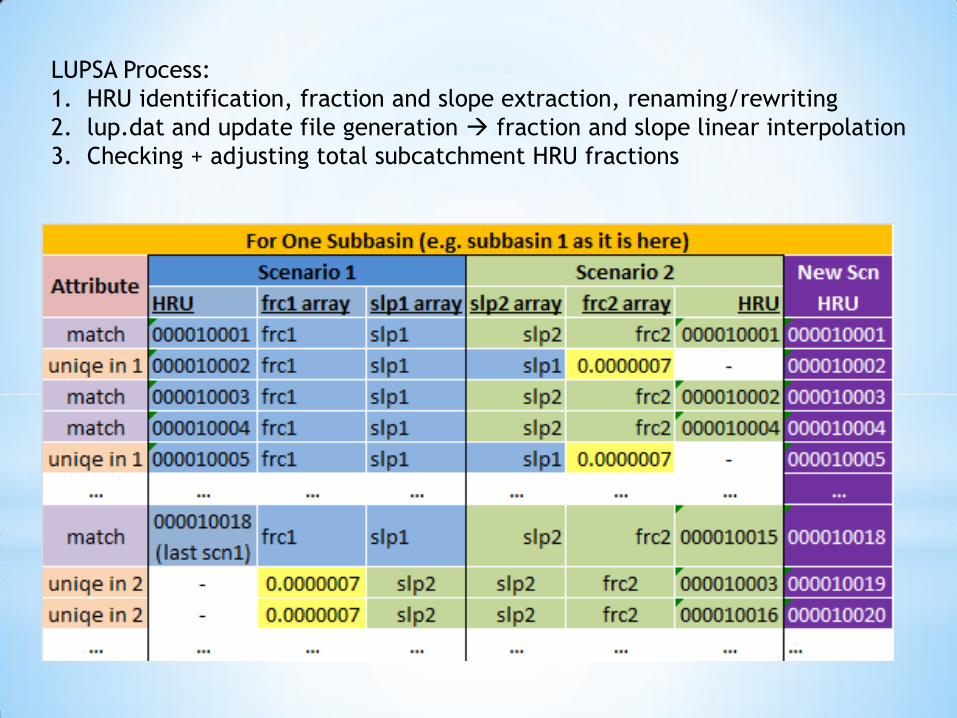
LUPSA Process:

1. HRU identification, fraction and slope extraction, renaming/rewriting

2. lup.dat and update file generation fraction and slope linear interpolation

3. Checking + adjusting total subcatchment HRU fractions

Example: 2 setups based on 2 LU inputs but one parameterisation

Common HRUs = 286

Unique HRUs 1 = 56

Unique HRUs 2 = 94

Unique HRUs: 34%

Program Language: Python

License: Open Source

OS: Windows (95+) and Linux

Running on: Command Line

GUI: .txt setup file

SWAT2009lu-slope.exe Fraction + slope update

SWAT2009lu-noslope.exe fraction update

SWAT2009lu-slope-slopelength.exe Fraction + slope + slope length update

Related modified SWAT Versions (by Ann van Griensven)

Conclusions

& Prospects

SWAT & LUC

Test Case &

LUPSA app.

LUPSA

Introduction

• Size: ~285 km²

• Elevation: 2176m-3986m

• Slope: up to 84%, ø = 16%

Data:

• Minor relation between

Rainfall Stations

• Poor Elevation – Rainfall

Relation

• Overrated discharge

measurements

• Fast Catchment response

Conclusions

& Prospects

SWAT & LUC

Test Case &

LUPSA app.

LUPSA

Introduction

Land use dynamics onwards artificial land use:

LUPSA application setup:

- Simulation period 1983-1993

- Annual land use updates from 1984 to 1993

- Land use inputs: remote sensing based shapes from

1972 and 2009 Conclusions

& Prospects

SWAT & LUC

Test Case &

LUPSA app.

LUPSA

Introduction

Results:

Simulation Calibration Validation

R2 NS R2 NS

Daily 89/90/92 0.39 0.39 0.26 0.24

Daily 84-87 0.53 0.52 0.43 0.41

Daily 73/74 0.49 0.36 0.25 0.22

Monthly 89/90/93 0.85 0.63 0.66 0.55

Monthly 84-87 0.8 0.8 0.79 0.77

Annual Average of Hydrological Components [mm]

LUPSA NoSlope LUPSA Slope Basic Model

Precipitation 1313.9 1313.9 1313.9

Surface Runoff 137.12 137.11 132.99

Lateral Flow 113.48 113.73 106.45

Groundwater Flow 442.86 442.65 438.05

REVAP 9.66 9.65 9.77

Deep Aquifer Recharge 24.06 24.05 23.57

Evapotranspiration 592.3 592.3 604.9

Annual Average

- Daily Flow Basic Model Fraction Change

Slope and Fraction

Change

Maximum 195.000 197.700 197.700

Arith. Mean 5.930 6.070 6.071

Median 3.111 3.246 3.246

Maximum Difference 8.170 8.170

Average Difference 0.331 0.332

Calibra

tion

Flo

w

Hydro

logy

Conclusions

& Prospects

SWAT & LUC

Test Case &

LUPSA app.

LUPSA

Introduction

Results:

Conclusions

& Prospects

SWAT & LUC

Test Case &

LUPSA app.

LUPSA

Introduction

Conclusions

Achievements:

1. An automated lup.dat generation helps the

implementation of LUC in SWAT

2. To fully address LUC in SWAT, arising HRUs (due to

LUC) should be addressed

3. Land use change might have a considerable impact

(case dependent) on the hydrology also within

decades

Prospective

1. Applying the tool in European Russia on agricultural

production

2. Checking the impact of dynamic LUC implementation

on the calibration of the new model

Test Case &

LUPSA app.

SWAT & LUC

Conclusions

& Prospects

LUPSA

Introduction

What else is going on

Alternative:

Another tool was developed by at the University of

Arkansas which uses another approach of setting up the

luc.dat file (SWAT2009_LUC)

Advantage: Setup directly based on land use input grid

Disadvantage:

- accounting only for matching HRUs

- no slope change implemented

- Abrupt updates on the dates of the input grids which

may causes problems with the amount of water an

nutrients in the HRU storages

Other works:

A on going research about the impact of land use change

on the model calibration at the UNESCO-IHE applying

both tools supervised by Ann van Griensven

Test Case &

LUPSA app.

SWAT & LUC

Conclusions

& Prospects

LUPSA

Introduction

Thank you for your attention!