integrating ms excel in engineering technology curriculum · university , and the educational...
TRANSCRIPT

Paper ID #11558
Integrating MS Excel in Engineering Technology Curriculum
Mr. Dustin Scott Birch, Weber State University
Dustin S. Birch possesses a Master of Science in Mechanical Engineering from the University of Utah, aBachelor of Science in Mechanical Engineering from the University of Utah, and an Associate of Sciencein Design and Drafting Engineering Technology from Ricks College. Birch is an Assistant Professor andProgram Coordinator in the Mechanical Engineering Technology Department at Weber State University.He also serves as the Chairman of the Board of the Utah Partnership for Education. He is a member ofthe American Institute of Aeronautics and Astronautics (AIAA) and American Society for EngineeringEducation (ASEE). Birch has over 20 years of experience in detail design, engineering, and engineeringmanagement in the aerospace and process equipment industries.
c©American Society for Engineering Education, 2015
Page 26.991.1

Integrating MS Excel into ET Curriculum
Page 26.991.2
Integrating MS Excel into ET Curriculum
Abstract: All STEM (Science, Technology, Engineering, and Mathematics) fields require
fundamental knowledge and application of problem simplification, model synthesis, calculations,
and results interpretation. As educators, it is our job to impart those skills to our students.
Classic education in Engineering Technology (ET) typically involves course work in the basic
sciences as well as mathematics. More advanced training is offered in specific disciplines
related to engineering such as solid mechanics, fluid mechanics, materials, machines and
mechanisms, etc.
Beginning in the last half of the twentieth century, computers and hand held calculators became
increasingly integrated in the technical problem solving process. What began as a means to
quickly and accurately perform mathematic calculations has evolved into very sophisticated
design, simulation, and analysis tools as computing power has increased exponentially over the
past few decades. Nearly all companies and educational institutions have adopted these
technological tools to solve engineering problems that only a few years ago would have been
impossible to solve with anything approaching the level of efficiency, sophistication, and
accuracy now possible.
Along with the power and flexibility of these modern software packages comes a high cost of
acquisition and maintenance, as well as demanding computer hardware requirements that
sometimes drive costs prohibitively high. Additionally, most of these high end software
packages come with a steep learning curve requiring specialized training to learn the intricacies
of the program. Many of these advanced software suites can require many months or even years
of continued use to master.
Contrary to the elaborate and often expensive software used in the design and analysis arena,
Microsoft (MS) Excel is bundled as part of the MS Office suite of software, typically available
on most computers used in educational and industry environments. In additional to being widely
available and comparatively inexpensive, MS Excel does not have strict hardware requirement to
operate correctly. MS Excel has been used in several courses taught in the Mechanical
Engineering Technology (MET) department to reinforce fundamental concepts, model problems
difficult to solve using more conventional means, reduce and interpret experimental data, and
provide a platform for students to formulate and apply engineering models and approaches to
solving various problems. To date, the effort to use MS Excel as an instructional tool has been
effective. Students are responding well to the instruction. Not only are they being exposed to
alternate approaches to problem solving, they are gaining a software skill that is very portable to
future jobs in the professional sector.
This paper will discuss the specific techniques used to integrate MS Excel into class curriculum.
It will also describe the various courses where MS Excel has been implemented at Weber State
Page 26.991.3

University, and the educational outcomes. Additionally, the paper includes step-by-step
examples explaining how to recreate two of the cited examples.
Background: In a traditional MET program, students will typically be required to successfully
complete courses in college algebra, trigonometry, and calculus. This foundation in mathematics
will become essential as they progress into engineering courses in solid mechanics, fluid
mechanics, materials, and machine design. Over the centuries that humans have been developing
the various branches of engineering science, equations have been derived with related systems of
units to describe the physical phenomena being modeled and described. Almost all technical
problems in science and engineering require quantified information to be manipulated into a
useful form, with potentially many calculations being performed to arrive at the final solution.
Almost without exception, in engineering coursework, students are instructed in the fundamental
science of a given subject, the governing equations, and techniques used to arrive at desired
solutions to problems. Typically this process involves evaluating the question being posed, and
deciding which equations are appropriate for formulating a solution. Once a strategy is
established, the students are taught how to interpret the known parameters, and set up the
appropriate mathematics to calculate an answer. Attention to such things as dimensional
consistency and units are also emphasized. Once a solution is arrived at, students are taught how
to evaluate the accuracy of the solution, as well as interpretation of the significance of the answer
as it relates to the question at hand. For the most part, conventional mathematics is employed to
perform the required calculations. If a closed form solution to the problem does not exist,
students are taught basic strategies to make assumptions to simplify the problem such that a
solution can be accomplished.
Alternately, if a problem has a level of uncertainty or sophistication beyond conventional
techniques, numerical or iterative schemes may be employed to achieve an approximate solution.
For these types of solutions, an electronic computer capable of billions of calculations per second
is an extremely useful tool. In fact, for most cases, solving problems of this nature without a
computer would be an impossible task. In select MET curriculum, using a computer to help
solve various engineering problems is implemented to achieve the following two educational
goals:
First, students develop a better understanding of the fundamental science and mathematics of a
particular problem, as they are required to construct a computational model.
Second, students gain a basic understanding of a specific software tool which is portable to
industry, thus making them more marketable and prepared to enter the work force.
For classes where computer software is employed, it is typical to use the customary commercial
codes that are available. Basic instruction into the operation of this software is presented as part
of the standard course curriculum. One required course (MET 3300 Computer Programming
Applications in MET) requires students to learn a high level programming language to formulate
Page 26.991.4
solutions to various engineering problems by coding a solution and running their software to
validate the approach. Hence, our students are given basic instruction in fundamental computer
programming as well as exposure to various specialized engineering software. The introduction
of MS Excel examples in select courses, is used to further expand students understanding of
possible analytical tools that can also be exploited to solve problems.
Discussion: With the rise of the electronic computer during the mid-twentieth century,
tremendous strides were made with regards to the speed, accuracy, and sophistication of
mathematic calculations. As computer technology continued to evolve, not only in lower costs
of acquisition and use, but in speed and the level of graphic display sophistication possible, very
advanced analysis and simulation software became increasingly available in engineering fields
both commercial and academic. At present, the market is full of useful software tools to assist in
performing engineering calculations.
In most modern engineering and engineering technology programs throughout institutions of
higher learning around the world, many of these commercial software codes have become staples
in degree curriculum. Software packages such as AutoCAD, SolidWorks, PTC Creo Elements
(formerly Pro/E), CATIA, NX (formerly Unigraphics), and many other are capable of not only
CAD modeling, but are useful tools for motion analysis and geometric simulation and
measurement. Many of these CAD tools have add on or bundled Finite Element Analysis (FEA)
or Computational Fluid Dynamics (CFD) software available. These advanced analytical tools
are capable of very complex simulations of structures, heat transfer, fluid mechanics, etc. In
addition to the CAD and analysis software, programs such as MathCAD, Mathmatica, Maple,
TK Solver, Matlab etc. offer advanced computational capabilities, calculation automation,
programing, and technical documentation functionality.
Detailed instruction in many of these various software packages is available in courses offered
throughout the curriculum provided in our program. Although, good foundational instruction is
provided in our various coursework, expert level mastery of most advanced engineering software
tools is beyond the scope of a typical undergraduate level class. Given the overall sophistication
of these software packages, learning to become proficient in their use requires a great deal of
experience. Most of these software packages take months or even years of use to become an
expert user. Many of these software suites also come with very high acquisition and
maintenance costs, and require very powerful computer hardware to operate correctly. As such,
they are not typically available in a wide fashion such as more common word processing or
spreadsheet software. Additionally, most of the mathematic and algorithm details occur behind
the scenes as the code executes, forcing the user to trust that programs are indeed functioning
correctly and providing an accurate solution. Hence, the user approaches the software as
somewhat of a “black box” by feeding in design parameters and trusting the corresponding
output to be correct. With the actual solution to the problem obscured as the software executes,
students get little or no exposure to the mechanics of the problem solving itself. They gain
valuable experience in setting up the appropriate simulation model with correct design
Page 26.991.5
assumptions and boundary conditions, and they are required to assess the accuracy and
correctness of the output solution, but have little or no visibility to the mechanics of the problem
solving.
As with all Mechanical Engineering and Mechanical Engineering Technology programs, a broad
and diverse curriculum in engineering science is required. As faculty, we are always
investigating better ways to introduce concepts, present correct approaches to problem solving,
and then assess student mastery and performance against learning outcomes. It is very valuable
in an educational setting, to not only present material and have students practice solutions, and
later be tested on those concepts, but to present information in alternate or unique ways so that
the students can have the best chance possible to comprehend the material and be able to utilize
it correctly. Using a simple, and commonly available software package, to present and practice
concepts in an ancillary way is just one way to assist in the learning process. Additionally, as
students transition out into industry, some of the high-level software tools used in school may not
always be available in the workplace, but MS Excel will most likely be available, and can
potentially be utilized as they have had former experience with it for solving technical problems.
It is the author’s experience, during multiple decades working in industry, for several different
companies, it was somewhat unlikely that a specific company may have, for example, a license
of MathCAD or a C++ compiler, but they were almost certain to have multiple licenses of MS
Excel that could be utilized for engineering analysis. Of course, the spreadsheet software is not
always capable of the level of sophistication required for certain problems or simulations, nor
should it be used that way, but in many cases it can be a very useful analysis tool with minimal
associated cost or complexity.
Application of MS Excel in Course Curriculum: As noted above, the use of high end
simulation tools can sometimes be overkill, and possibly counterproductive in a classroom
instruction environment. The goal in education is to not only teach a student how to achieve a
correct solution, but to thoroughly understand and appreciate the science and mathematics used
to formulate the problem. Using computers and software to quickly, and in a simple way,
communicate principles and problem solving techniques, is a useful bridge between high level
computing and traditional pencil and paper analysis.
MS Excel can be a low cost and relatively simple tool used to demonstrate and reinforce
concepts in the classroom, as well as encourage students to build simulations from scratch,
utilizing the basic equations to build higher level solutions to engineering problems. Although
the software is best known for its financial and budgetary uses, it actually has fairly sophisticated
computational capabilities as well. In addition to its mathematical function library, the software
is easy to use, and has reasonable graphing functionality. Beyond the core functionality, the
software also has basic logic and data analysis features. Also available to the more experienced
user is a programming interface using a Visual Basic shell to create more elaborate applications.
Most importantly, the software is readily available, as it ships bundled in the standard MS Office
Page 26.991.6
suite for a relatively low cost. The entire MS Office suite is available for a few hundred dollars,
as compared to thousand or tens of thousands of dollars for other engineering analysis suites.
According to data published by Microsoft on its website, it is estimated that MS Office is used
by more than one billion people worldwide.1 Therefore, it is probably one of the most
commonly available software packages in existence. For this reason, it was chosen as a good
candidate for the simple engineering model examples presented. Other low-cost or shareware
software does exist that is comparable in power and functionality to MS Excel. An example of
this would be Google Sheets, which is a free spreadsheet software developed by Google.
However, MS Excel does have the largest marketplace exposure and overall usage by
educational institutions as well as in industry. Hence, it was chosen as the software tool of
choice for various classroom examples.
MS Excel is implemented in various course curriculum to introduce students to its flexibility and
available functionality as it relates to various engineering problems. It is also used to reinforce
various concepts, by having students walk through the synthesis of a problem, and program the
spreadsheet to solve it, thus reinforcing their problem solving strategies. It is not intended to be
a replacement to some of the high end design and analysis tools. It is intended to be used as a
possible alternative, in some cases, to these software packages, and more often, a companion to
be used in conjunction with more sophisticated engineering software. Students in the MET
program are trained in other software, and are expected to develop knowledge and skills using
various CAD and FEA packages. MS Excel is used to illustrate various concepts, and improve
visibility to possible alternative solutions. Without elaborate custom programming, MS Excel
will only be able to handle simpler problem solving, and its core functionality would certainly
not replace any commercial codes that are highly specialized, and used for high-level
engineering design and analysis. However, in some cases, it can be used as a cost effective,
simple, and quite useful tool to perform analysis or automate tedious and error prone tasks and
calculations.
Over the past four years, several MS Excel examples and projects have been implemented into
the MET curriculum to illustrate concepts being taught in various courses. Additionally,
periodic student assignments using MS Excel have been used to further reinforce basic concepts
as well as give cursory instruction into the functionality and use of spreadsheet software in an
engineering environment.
The courses where MS Excel has been implemented were identified as candidates for this
approach due to the nature of the course material and its possible applicability in a spreadsheet
example. Criteria included such things as reasonable mathematic simplicity within the
capabilities of the spreadsheet core functionality, limited requirements for graphic output, and
fairly limited programming requirements to achieve a solution. Of interest also were potentially
tedious or error prone calculation processes, where a spreadsheet would be particularly helpful,
especially in the case of iterative design studies or high volume repetitive calculations. These
types of subjects within various courses were identified as possible good candidates for a
Page 26.991.7
spreadsheet example, and follow-on student projects to create their own functioning spreadsheet
models. It was also intended to use MS Excel in several different courses with diverse subject
matter to accomplish three goals:
First, illustration of the possible diverse applications of the software.
Second, continued reinforcement and practice in software skills.
Third, to reinforce the technical and mathematical background of various subjects, as well as
practice problem solving skills.
It is important to note, that where appropriate, high end analysis tools were demonstrated in
conjunction with MS Excel examples to illustrate their power and functionality, and to validate
possible simpler solutions to the exact same problem.
Prior to the introduction of the MS Excel projects in various Mechanical Engineering
Technology courses, it has been observed that most students have some basic knowledge of MS
Excel, but others are relative novices. It has also been noted that even students who have some
advance knowledge of the software, often have no idea of the flexibility and functionality
available to perform engineering analysis prior to exposure in the MET classroom environment.
Based on the course selection criteria noted above, presented below are examples of various
courses where the MS Excel teaching tool or projects have been used:
MET 3400 – Machine Design: Two specific MS Excel examples have been developed for use
in the upper division machine design course required of all Mechanical, Manufacturing, and
Design students.
The first spreadsheet example is used to illustrate combined stress fields, specifically
transformed stress, principal stresses, and maximum shear stress. Prior to the machine design
class, students are required to successfully complete a statics and strength of materials course. In
that course, basic strengths of materials concepts are taught. However, detailed instruction in
stress transformation and principal stress is not presented.
Following classroom introduction of transformed stress using a traditional lecture, and numerous
example problems, the stress element rotation spreadsheet is presented. The learning outcome
expected from demonstrating this spreadsheet is for the students to better understand the
fundamental concepts of transformed stress as well as its relationship to the principal stress
equations. A copy of the transformed stress spreadsheet is made available to the students after
its classroom introduction. They are then encouraged to interrogate the programming as well as
to use it as a means to check their homework problems.
The spreadsheet is designed to show a 2-D plane stress element incrementally rotated through
180 degrees with the representative transformed stress calculated and plotted on a graph. The
Page 26.991.8
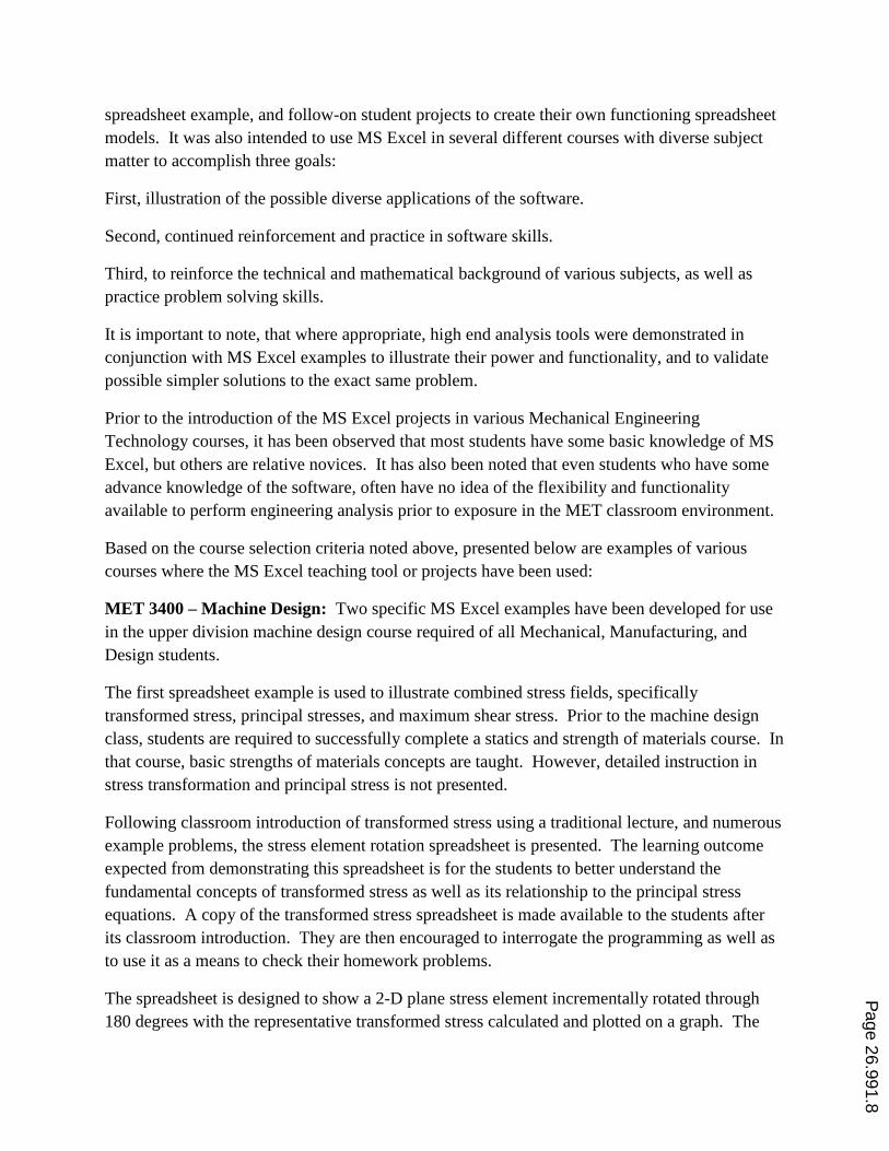
user inputs the multi-axial stress field (σx, σy, τxy) into the designated cells. Utilizing the user
supplied stress values, the spreadsheet then calculates the transformed stress based on the
rotation angle (θ) using the following equations: 2
)2cos()2sin(2
)2sin()2cos(22
)2sin()2cos(22
''
'
'
xy
yx
yx
xy
yxyx
y
xy
yxyx
x
The angle is incremented by one degree per step, and the corresponding transformed stress
values are tabulated. Note that the corresponding angle in radians, rather than degrees, is
calculated as well. This is due to the fact that MS Excel only performs trigonometric functions
using radians.
The tabulated values of transformed stresses are then used to create and x-y scatter plot
illustrating the transformed stress values as a function of rotation angle. The spreadsheet also
searches through the iterative results to determine the maximum and minimum normal stresses
(1st & 2nd Principal Stress) as well as the approximate maximum shear stress. Adjacent to the
approximate solution, the exact results are presented. The exact principal stress solution is
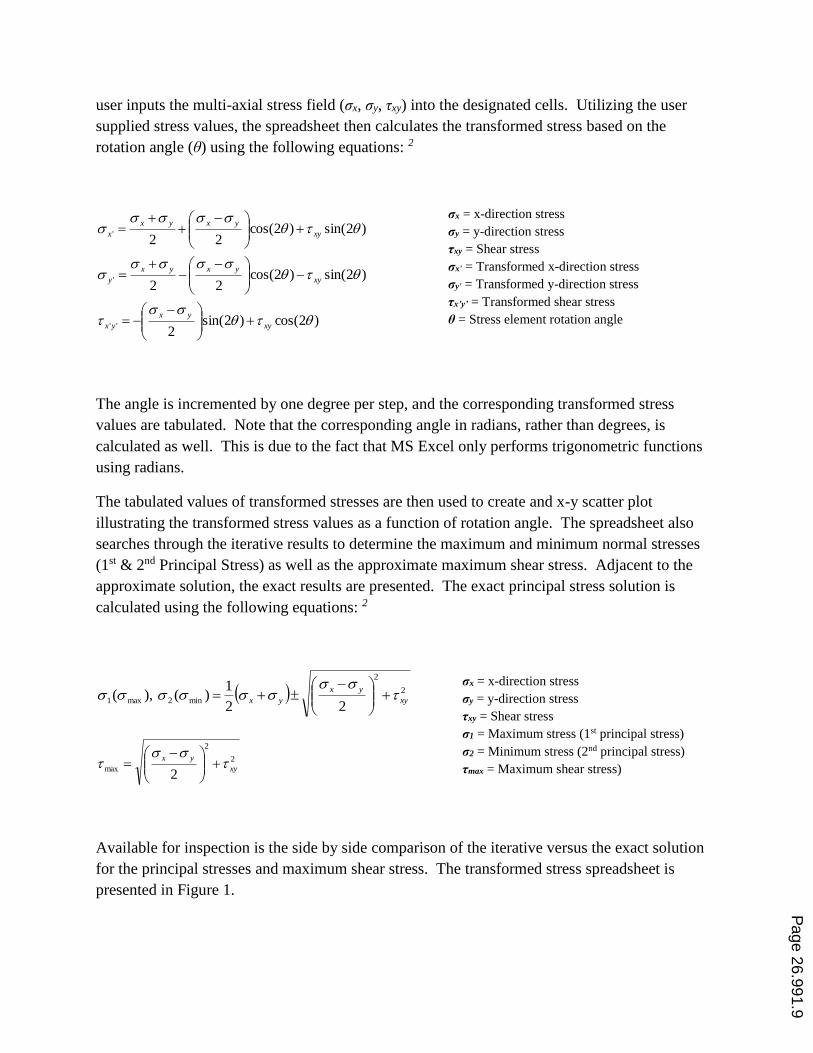
calculated using the following equations: 2
2
2
min2max122
1)(),( xy
yx
yx
2
2
max2
xy
yx
Available for inspection is the side by side comparison of the iterative versus the exact solution
for the principal stresses and maximum shear stress. The transformed stress spreadsheet is
presented in Figure 1.
σx = x-direction stress
σy = y-direction stress
τxy = Shear stress
σx' = Transformed x-direction stress
σy' = Transformed y-direction stress
τx’y’ = Transformed shear stress
θ = Stress element rotation angle
σx = x-direction stress
σy = y-direction stress
τxy = Shear stress
σ1 = Maximum stress (1st principal stress)
σ2 = Minimum stress (2nd principal stress)
τmax = Maximum shear stress)
Page 26.991.9
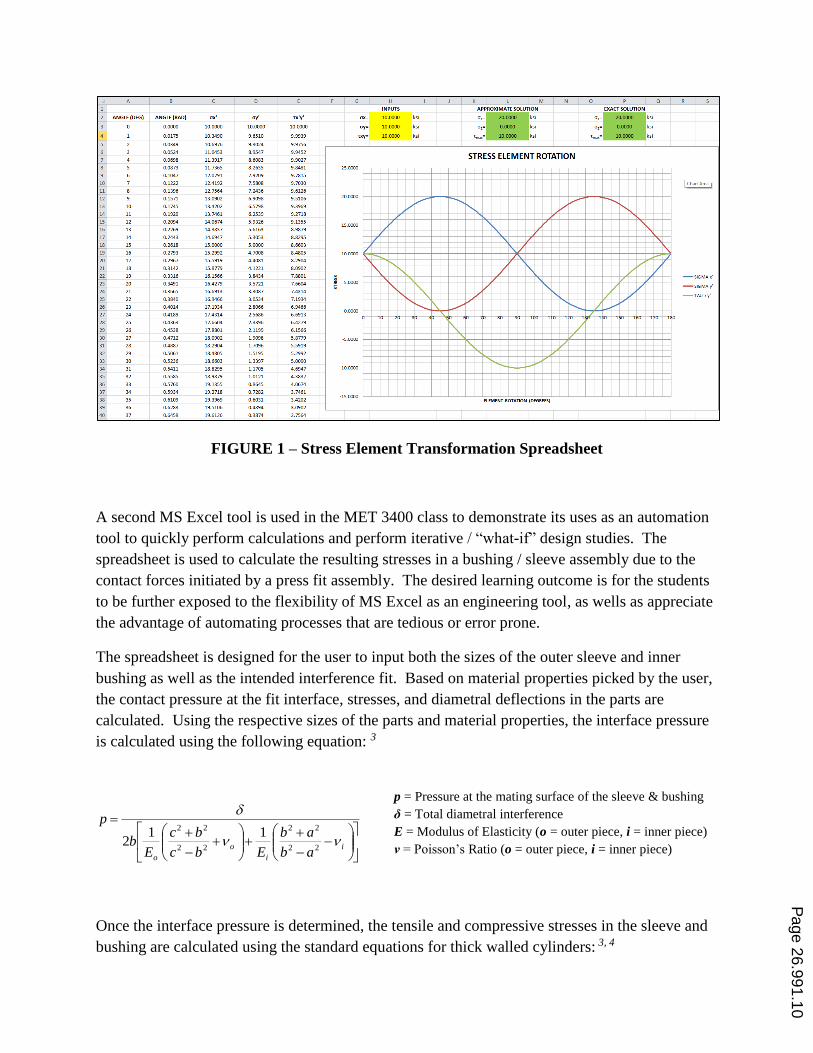
FIGURE 1 – Stress Element Transformation Spreadsheet
A second MS Excel tool is used in the MET 3400 class to demonstrate its uses as an automation
tool to quickly perform calculations and perform iterative / “what-if” design studies. The
spreadsheet is used to calculate the resulting stresses in a bushing / sleeve assembly due to the
contact forces initiated by a press fit assembly. The desired learning outcome is for the students
to be further exposed to the flexibility of MS Excel as an engineering tool, as wells as appreciate
the advantage of automating processes that are tedious or error prone.
The spreadsheet is designed for the user to input both the sizes of the outer sleeve and inner
bushing as well as the intended interference fit. Based on material properties picked by the user,
the contact pressure at the fit interface, stresses, and diametral deflections in the parts are
calculated. Using the respective sizes of the parts and material properties, the interface pressure
is calculated using the following equation: 3
i
i
o
o ab
ab
Ebc
bc
Eb
p
22
22
22
22 112
Once the interface pressure is determined, the tensile and compressive stresses in the sleeve and
bushing are calculated using the standard equations for thick walled cylinders: 3, 4
p = Pressure at the mating surface of the sleeve & bushing
δ = Total diametral interference
E = Modulus of Elasticity (o = outer piece, i = inner piece)
ν = Poisson’s Ratio (o = outer piece, i = inner piece)
Page 26.991.10
22
22
bc
bcpob
22
22
ab
abpib
22
22
bc
pboc
22
22
ab
pbia
The deflection of the inner and outer rings is calculated using the following equations: 3
o
o
obc
bc
E
bp
22
222
i
i
iab
ab
E
bp
22
222
Additionally, this spreadsheet project illustrates the use of imported graphics to display a
schematic of the assembly being analyzed, as well as the applicable equations used in the
spreadsheet simulation. The intent of these features is to illustrate steps that can be employed
during the set-up of the spreadsheet to make it more user friendly. Additionally, the spreadsheet
also includes simple instructions as to the use as well as standardization of colors (yellow for
user inputs and green for calculated values) to further aid the user as to the correct use of the
tool. The press-fit calculator spreadsheet is presented in Figure 2.
σob = Tensile stress in outer piece (at interface)
σib = Compressive stress in inner piece (at interface)
σoc = Tensile stress in outer piece (at OD)
σia = Compressive stress in inner piece (at ID)
a = Inner radius of inner piece
b = Interface radius
c = Outer radius of outer piece
p = Pressure at the mating surface of the sleeve & bushing
δo = Total diametral deflection (outer piece)
δi = Total diametral deflection (inner piece)
p = Pressure at the mating surface of the sleeve & bushing
a = Inner radius of inner piece
b = Interface radius
c = Outer radius of outer piece
E = Modulus of Elasticity (o = outer piece, i = inner piece)
ν = Poisson’s Ratio (o = outer piece, i = inner piece)
Page 26.991.11
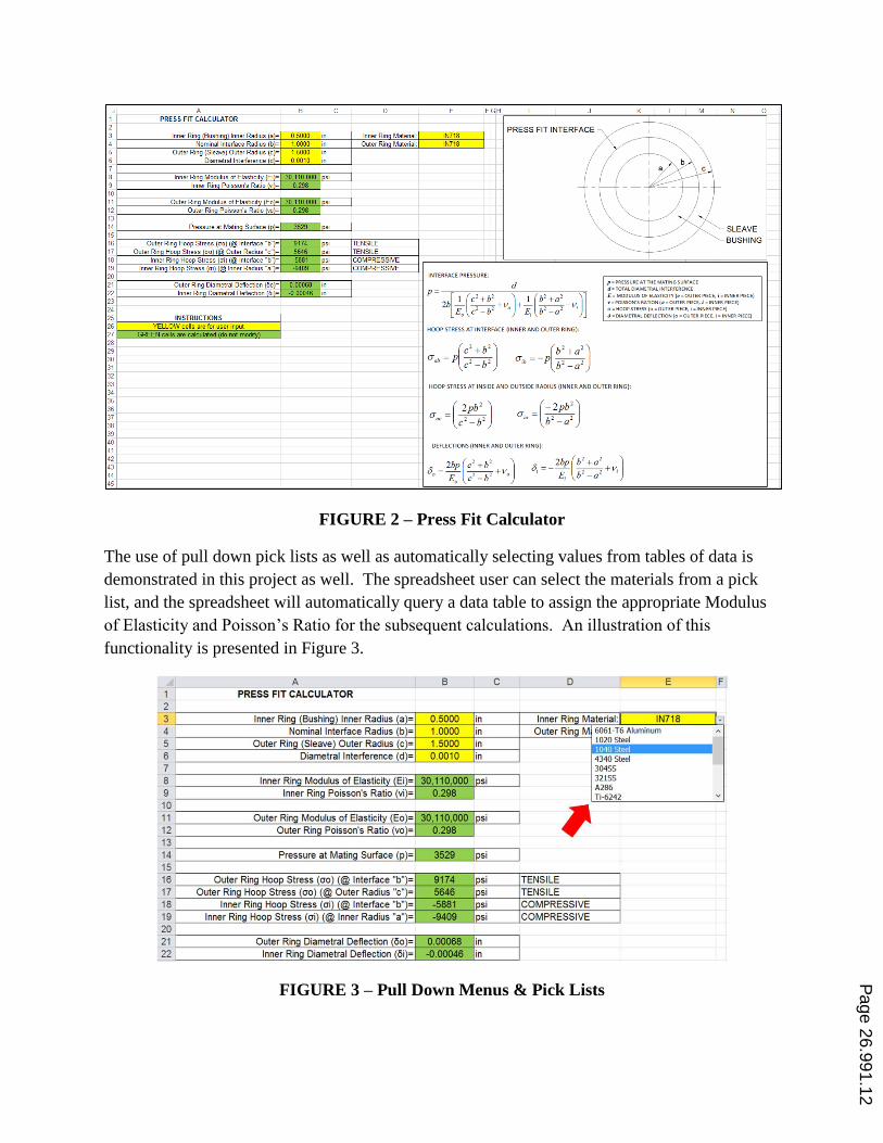
FIGURE 2 – Press Fit Calculator
The use of pull down pick lists as well as automatically selecting values from tables of data is
demonstrated in this project as well. The spreadsheet user can select the materials from a pick
list, and the spreadsheet will automatically query a data table to assign the appropriate Modulus
of Elasticity and Poisson’s Ratio for the subsequent calculations. An illustration of this
functionality is presented in Figure 3.
FIGURE 3 – Pull Down Menus & Pick Lists
Page 26.991.12
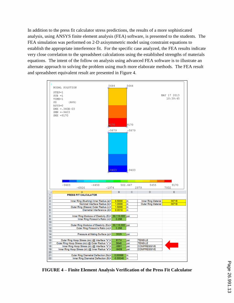
In addition to the press fit calculator stress predictions, the results of a more sophisticated
analysis, using ANSYS finite element analysis (FEA) software, is presented to the students. The
FEA simulation was performed on 2-D axisymmetric model using constraint equations to
establish the appropriate interference fit. For the specific case analyzed, the FEA results indicate
very close correlation to the spreadsheet calculations using the established strengths of materials
equations. The intent of the follow on analysis using advanced FEA software is to illustrate an
alternate approach to solving the problem using much more elaborate methods. The FEA result
and spreadsheet equivalent result are presented in Figure 4.
FIGURE 4 – Finite Element Analysis Verification of the Press Fit Calculator
Page 26.991.13
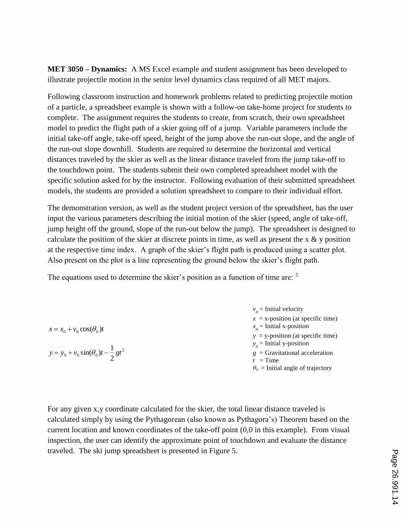
MET 3050 – Dynamics: A MS Excel example and student assignment has been developed to
illustrate projectile motion in the senior level dynamics class required of all MET majors.
Following classroom instruction and homework problems related to predicting projectile motion
of a particle, a spreadsheet example is shown with a follow-on take-home project for students to
complete. The assignment requires the students to create, from scratch, their own spreadsheet
model to predict the flight path of a skier going off of a jump. Variable parameters include the
initial take-off angle, take-off speed, height of the jump above the run-out slope, and the angle of
the run-out slope downhill. Students are required to determine the horizontal and vertical
distances traveled by the skier as well as the linear distance traveled from the jump take-off to
the touchdown point. The students submit their own completed spreadsheet model with the
specific solution asked for by the instructor. Following evaluation of their submitted spreadsheet
models, the students are provided a solution spreadsheet to compare to their individual effort.
The demonstration version, as well as the student project version of the spreadsheet, has the user
input the various parameters describing the initial motion of the skier (speed, angle of take-off,
jump height off the ground, slope of the run-out below the jump). The spreadsheet is designed to
calculate the position of the skier at discrete points in time, as well as present the x & y position
at the respective time index. A graph of the skier’s flight path is produced using a scatter plot.
Also present on the plot is a line representing the ground below the skier’s flight path.
The equations used to determine the skier’s position as a function of time are: 5
tvxx )cos( 000
2
0002
1)sin( gttvyy
For any given x,y coordinate calculated for the skier, the total linear distance traveled is
calculated simply by using the Pythagorean (also known as Pythagora’s) Theorem based on the
current location and known coordinates of the take-off point (0,0 in this example). From visual
inspection, the user can identify the approximate point of touchdown and evaluate the distance
traveled. The ski jump spreadsheet is presented in Figure 5.
v0 = Initial velocity
x = x-position (at specific time)
x0 = Initial x-position
y = y-position (at specific time)
y0 = Initial y-position
g = Gravitational acceleration
t = Time
θo = Initial angle of trajectory
Page 26.991.14
FIGURE 5 – The Ski Jump Problem
MET 2500 – Modern Engineering Technologies: An example of calculating the motion of a
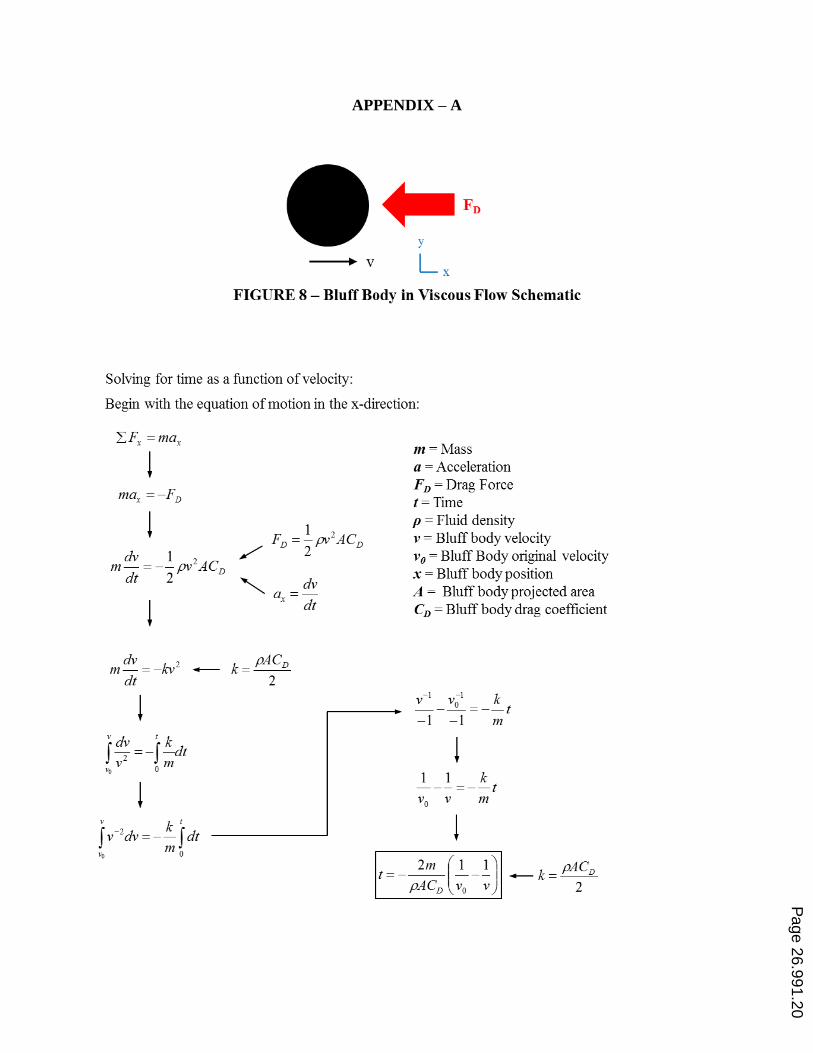
bluff body moving through a viscous fluid is used in a lower division engineering class to
illustrate the effects of drag force on a body moving in a fluid. The MET 2500 class is intended
to be a survey of modern technology and its applications in engineering. Modules are taught on
subjects such as power generation, transportation technologies, materials, advanced
manufacturing, and high technology engineering tools.
In the transportation technologies module, a lecture is taught regarding drag forces on aircraft,
trains, and automobiles. The theory and mathematics of calculating drag are derived and
presented. A spreadsheet example is used to further reinforce these concepts and principles.
Following review of the spreadsheet simulation, the students are assigned a special project to
create their own spreadsheet simulation of a particular problem.
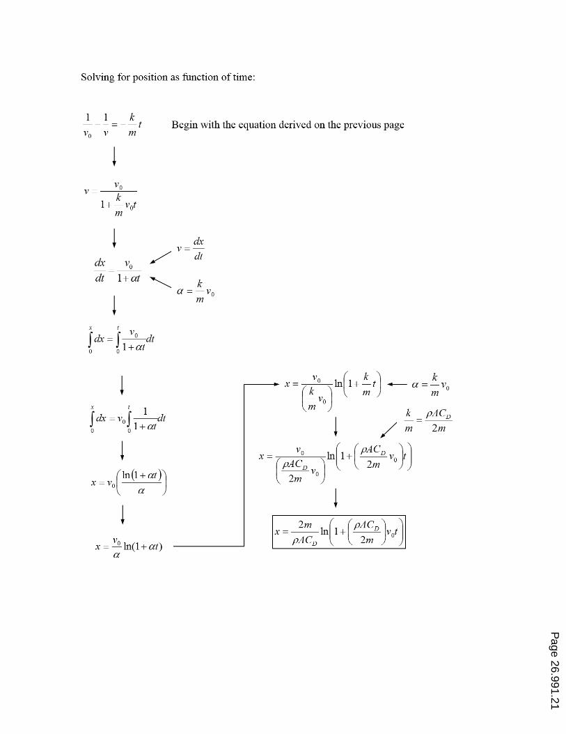
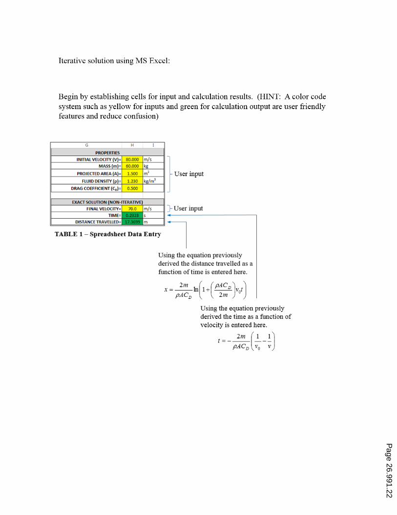
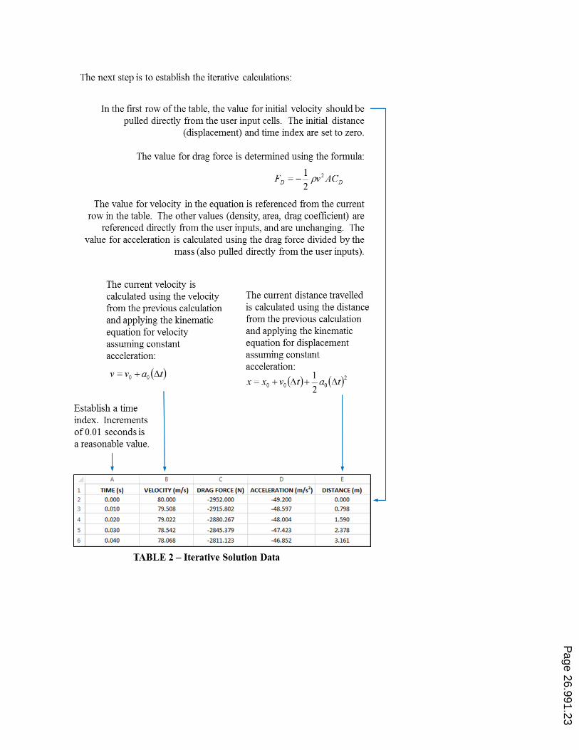
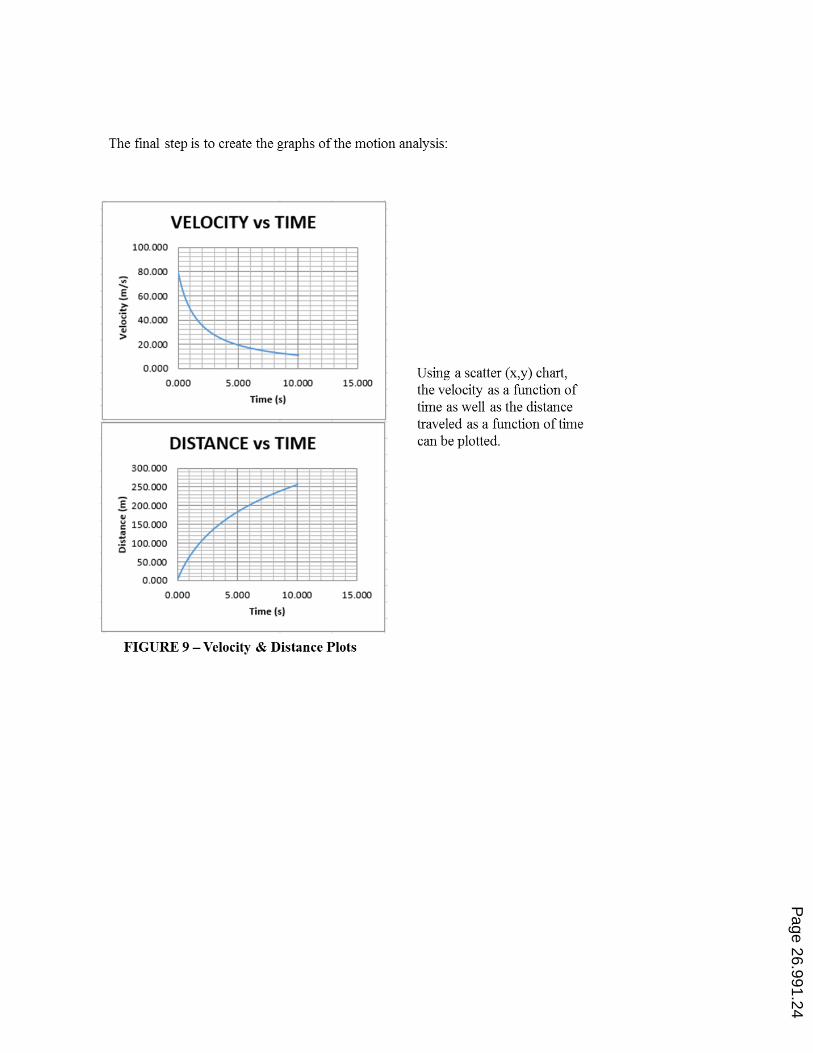
A closed form solution predicting the object motion requires solving differential equations, is
beyond the scope of the required prerequisites for the course. The derivation of the solution is
presented to the class to illustrate the mathematic complexity involved. Following the
presentation of the long solution, the spreadsheet is demonstrated. The spreadsheet basically
assumes constant acceleration for small time intervals. Assuming constant acceleration over
Page 26.991.15
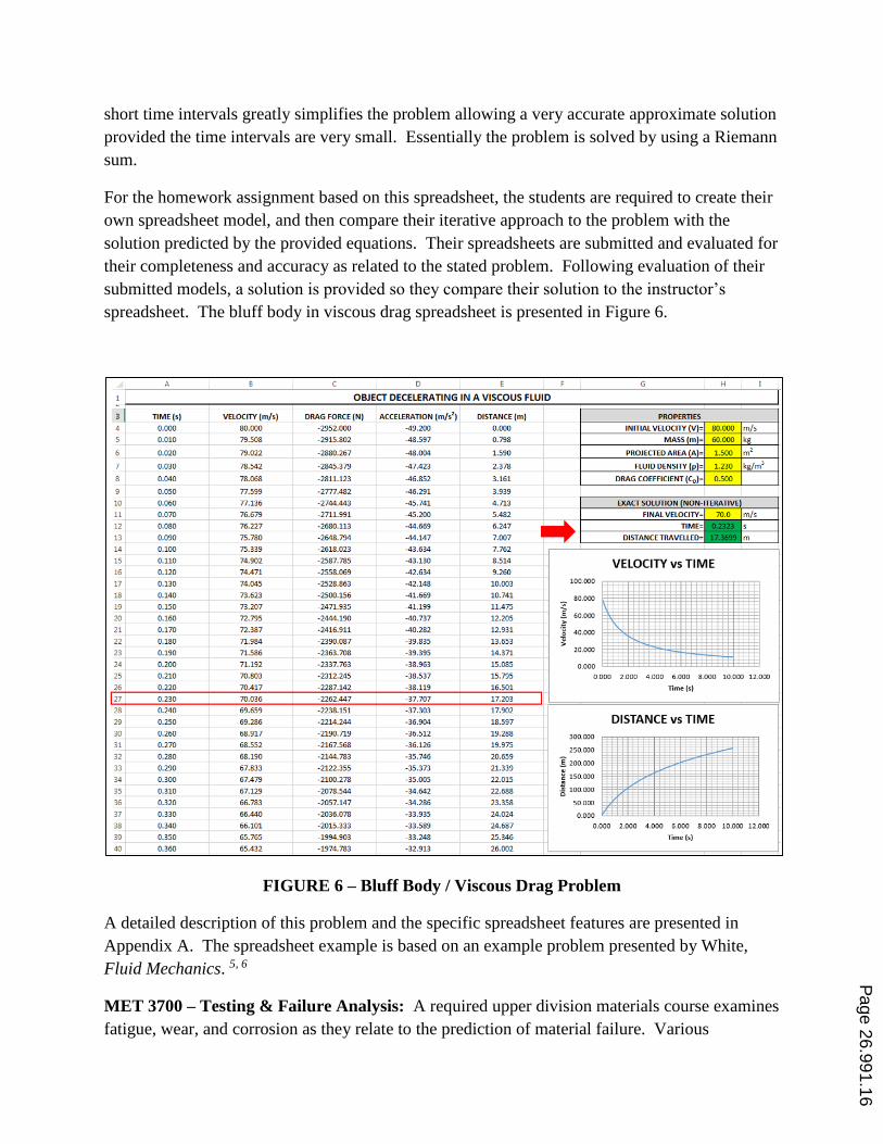
short time intervals greatly simplifies the problem allowing a very accurate approximate solution
provided the time intervals are very small. Essentially the problem is solved by using a Riemann
sum.
For the homework assignment based on this spreadsheet, the students are required to create their
own spreadsheet model, and then compare their iterative approach to the problem with the
solution predicted by the provided equations. Their spreadsheets are submitted and evaluated for
their completeness and accuracy as related to the stated problem. Following evaluation of their
submitted models, a solution is provided so they compare their solution to the instructor’s
spreadsheet. The bluff body in viscous drag spreadsheet is presented in Figure 6.
FIGURE 6 – Bluff Body / Viscous Drag Problem
A detailed description of this problem and the specific spreadsheet features are presented in
Appendix A. The spreadsheet example is based on an example problem presented by White,
Fluid Mechanics. 5, 6
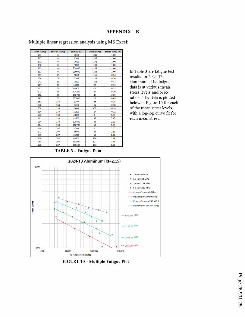
MET 3700 – Testing & Failure Analysis: A required upper division materials course examines
fatigue, wear, and corrosion as they relate to the prediction of material failure. Various
Page 26.991.16
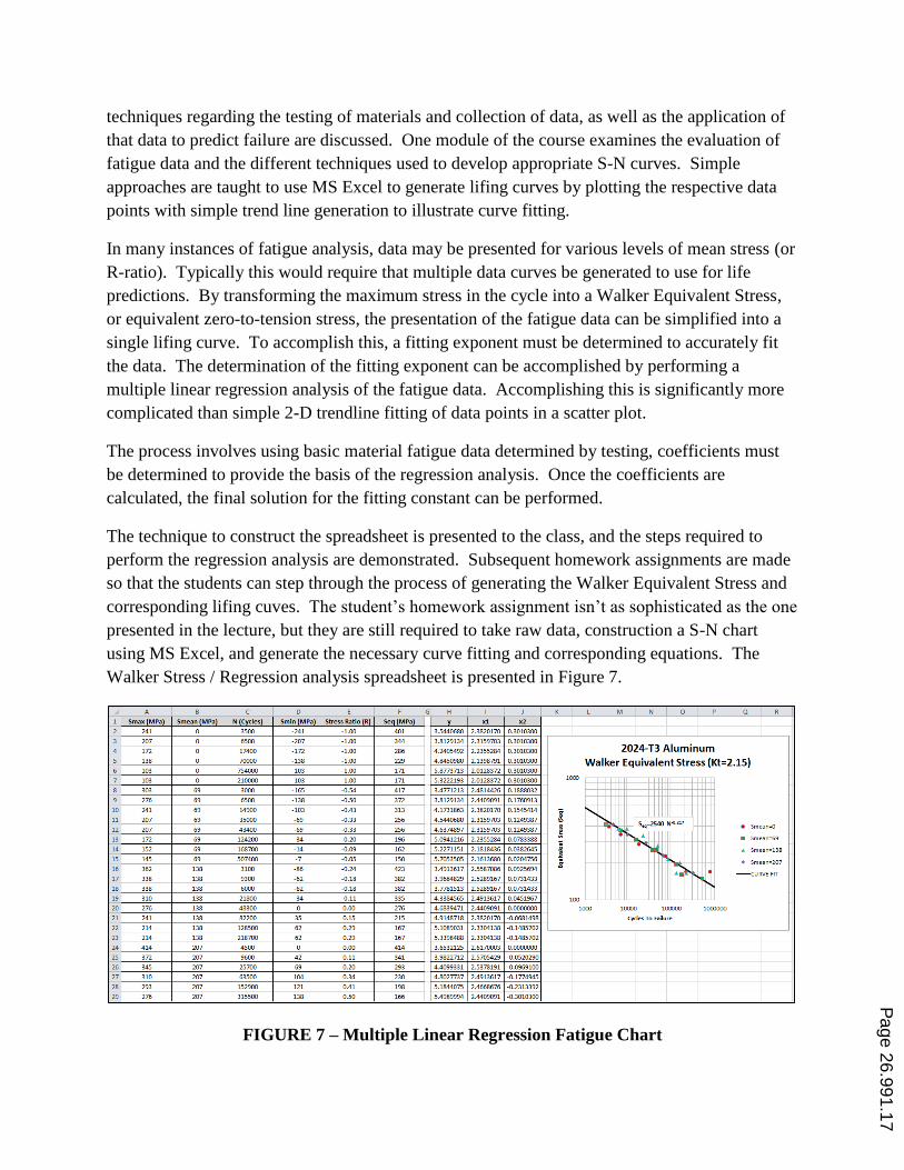
techniques regarding the testing of materials and collection of data, as well as the application of
that data to predict failure are discussed. One module of the course examines the evaluation of
fatigue data and the different techniques used to develop appropriate S-N curves. Simple
approaches are taught to use MS Excel to generate lifing curves by plotting the respective data
points with simple trend line generation to illustrate curve fitting.
In many instances of fatigue analysis, data may be presented for various levels of mean stress (or
R-ratio). Typically this would require that multiple data curves be generated to use for life
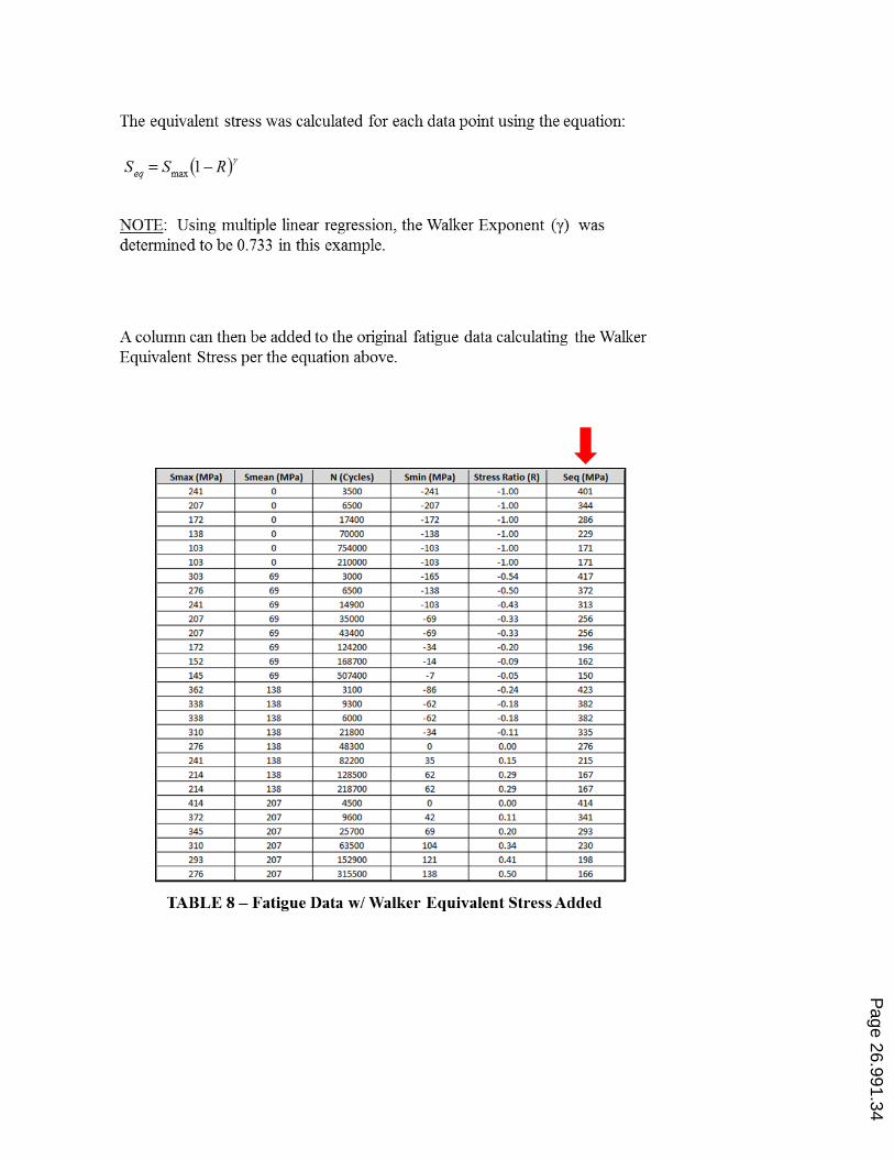
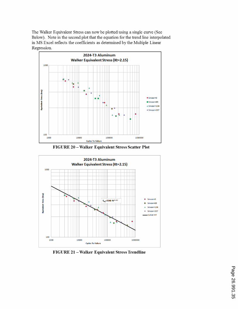
predictions. By transforming the maximum stress in the cycle into a Walker Equivalent Stress,
or equivalent zero-to-tension stress, the presentation of the fatigue data can be simplified into a
single lifing curve. To accomplish this, a fitting exponent must be determined to accurately fit
the data. The determination of the fitting exponent can be accomplished by performing a
multiple linear regression analysis of the fatigue data. Accomplishing this is significantly more
complicated than simple 2-D trendline fitting of data points in a scatter plot.
The process involves using basic material fatigue data determined by testing, coefficients must
be determined to provide the basis of the regression analysis. Once the coefficients are
calculated, the final solution for the fitting constant can be performed.
The technique to construct the spreadsheet is presented to the class, and the steps required to
perform the regression analysis are demonstrated. Subsequent homework assignments are made
so that the students can step through the process of generating the Walker Equivalent Stress and
corresponding lifing cuves. The student’s homework assignment isn’t as sophisticated as the one
presented in the lecture, but they are still required to take raw data, construction a S-N chart
using MS Excel, and generate the necessary curve fitting and corresponding equations. The
Walker Stress / Regression analysis spreadsheet is presented in Figure 7.
FIGURE 7 – Multiple Linear Regression Fatigue Chart
Page 26.991.17
A detailed description of this problem and the specific spreadsheet features are presented in
Appendix B. The spreadsheet example is based on an example problem presented by Dowling,
Mechanical Behavior of Materials. 7
Conclusions: The effort to implement MS Excel into to various MET course curriculum has
been successful. Many students have commented that the simulation spreadsheets have been
very helpful in reinforcing various concepts. They have also expressed appreciation in gaining
further instruction in how to leverage available technology for their specific skill sets in
engineering science. Some students who are currently employed in industry have reported that
they have used what they learned in working with MS Excel in our courses to improve their
efficiency on the job by implementing automated spreadsheet tools in the workplace. Some of
the projects developed for the various courses have been shared between faculty members, and
interest has been shown in how to further develop other examples and how to integrate them into
other course curriculum.
The addition of the MS Excel examples to various courses was done in the spirit of continuous
improvement advocated by ABET. It is the observation, based on student feedback and
instructor opinion, that this effort has improved understanding and retention of some key
engineering concepts as well as demonstrated alternate approaches to problem solving.
However, controlled studies that quantify the overall effect of the MS Excel integration have not
yet been conducted.
Although MS Excel is quite powerful, with a broad range of appliation in engineering science, it
is definitely not the only, or best solution, in many cases. In fact, its broad scope of functionality
applicable in many different unrelated disciplines does also create many limitations as it is not
specialized enough to be useful in many cases. For example, the graphing and output display
functionality is constrained to specific families of charts and graphs, with little built in
functionality to change these, especially in the 3-D presentation of data. Additionally, complex
itterative solutions can be difficult to perform without additional programming in Visual Basic.
The built-in logic features are adequate in many cases, but can also be somewhat limiting when
attempting to implement very complicated decision making into spreadsheet model.
As such, the MS Excel software does not have the inherit power and flexibility of high level
programming codes or other more specialized tools. Many of these limitations are pointed out,
and students are instructed to analyze what may be the best possible computing solution to the
problem at hand, understanding that MS Excel may not lend itself well to a particular problem.
Recommendations: Although feedback from students regarding the use of MS Excel in various
coursework has been overall positive, there is an opportunity to quantify and study the
measureable effect the instruction is having on learning outcomes. Future efforts would involve
the addition of new MS Excel simulations into coursework where it makes sense to do so.
Additionally, it would be beneficial to attempt to better quantify through a statistical study the
Page 26.991.18

specific benefits of the additional instruction afforded by the various spreadsheet examples and
student projects.
Future efforts would attempt to evaluate the mastery of a particular concept prior to initiating a
MS Excel programming example, and then measure any contribution to learning a specific
spreadsheet example and project has. Hard data would be collected relative to specific problems
given on exams, and then re-tested after students have been required to complete a specific
spreadsheet example to verify that the concept mastery has been improved. A specific example
would be to quiz the student’s mastery of a particular concept. Then create a control group using
traditional homework problems. A second study group would be assigned a spreadsheet
programming project. A follow-up exam will assess any learning advantage the spreadsheet
programming project may have over traditional homework problems alone.
As noted above, some of the classes that use MS Excel examples use them only as instructional
aids, where others actually have homework assignments for students to create their own working
spreadsheet models, where applicable, it would be best for all in-class examples to include a
representative student project as a hands-on learning exercise. This will also be a potential future
improvement.
Page 26.991.19
APPENDIX – A
Page 26.991.20
Page 26.991.21
Page 26.991.22
Page 26.991.23
Page 26.991.24
APPENDIX – B
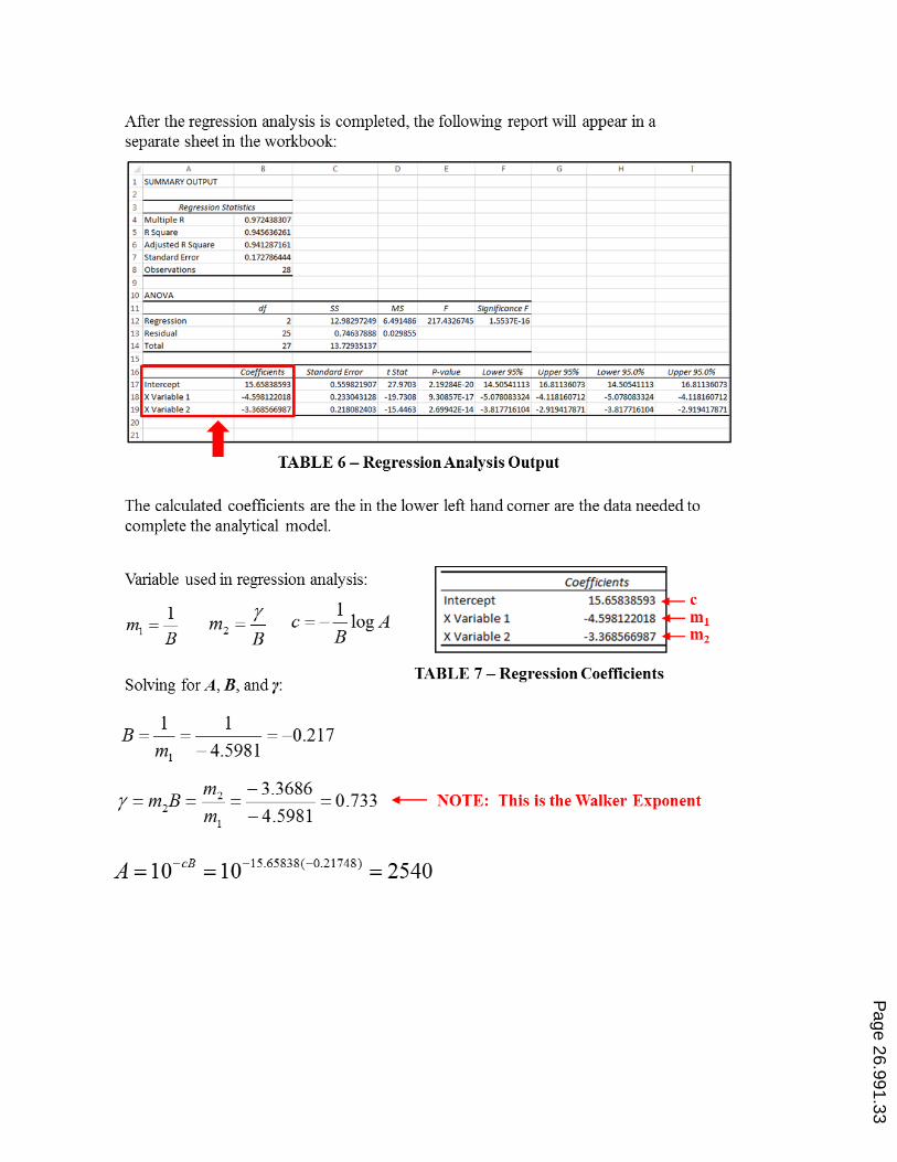
Multiple linear regression analysis using MS Excel:
Page 26.991.25
The walker equivalent stress can be used to transform fatigue data with any mean stress
/ stress ratio (r) into an equivalent zero to tension stress ratio (R=0).
The Walker equation is:
RSSeq 1max
Seq
= Walker Stress
Smax
= Maximum Stress
R = Stress Ratio (Smin
/Smax
)
γ = Fitting Exponent
The fitting exponent (γ) is determined by fitting the data to a single trend line using
multiple linear regression.
To solve for the Walker Exponent (γ), a multiple linear regression must be performed
to fit the data.
The basic form of the equation is:
RSAN B
f 1max
This expression can be reorganized into:
)1log(logloglog max RSNBA f
Rearranging the equation yields:
AB
RB
SB
N f log1
)1log(log1
log max
The unknowns we are curve
fitting are A, B, and γ.
The equation is of the form:
Where:
fNy logmax1 log Sx )1log(2 Rx
Bm
11
Bm
2
AB
c log1
cxmxmy 2211
Page 26.991.26
y is the dependent variable that is a function of the slope values, independent variables
(x) and the intercept
m values are slopes for each value of x
x values are the independent variables
c is the intercept
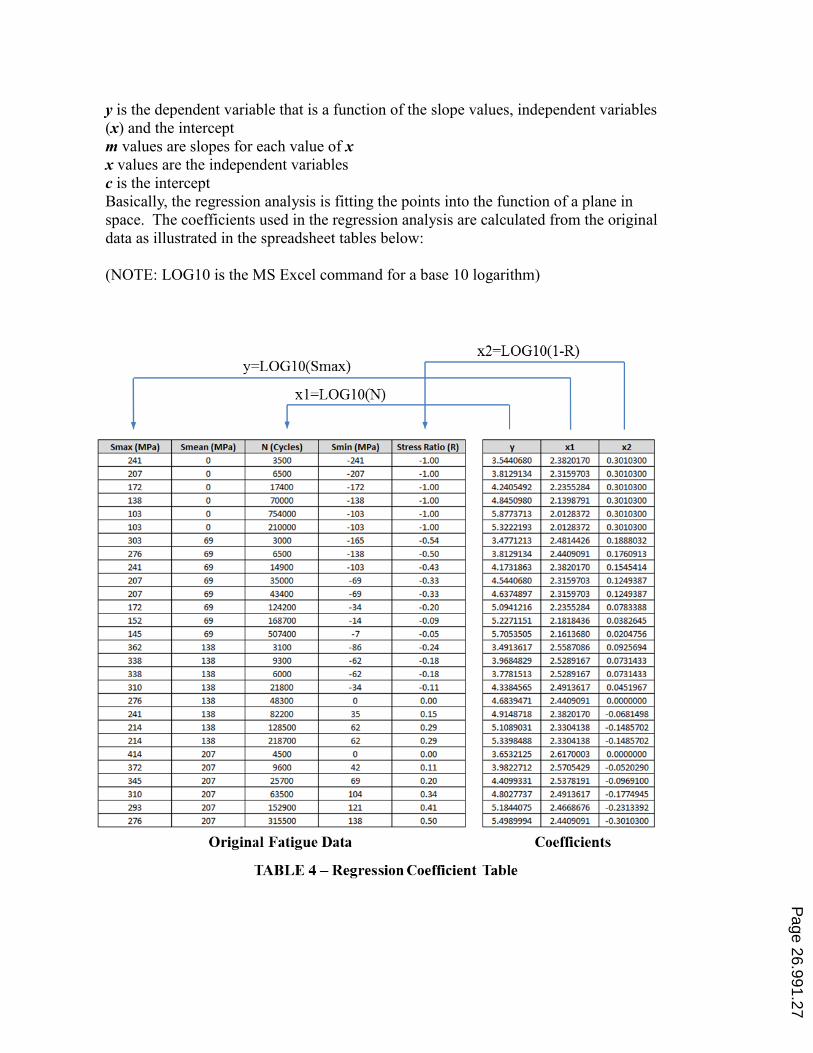
Basically, the regression analysis is fitting the points into the function of a plane in
space. The coefficients used in the regression analysis are calculated from the original
data as illustrated in the spreadsheet tables below:
(NOTE: LOG10 is the MS Excel command for a base 10 logarithm)
Page 26.991.27
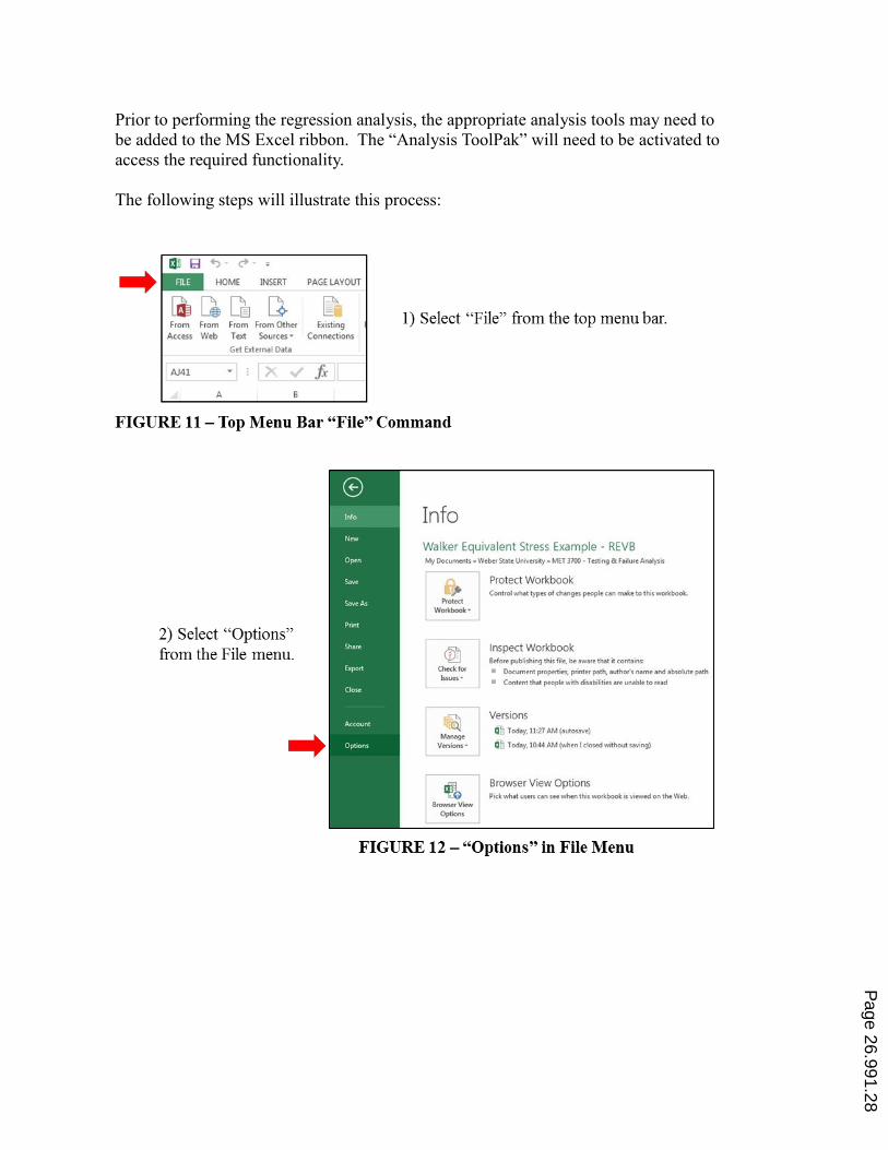
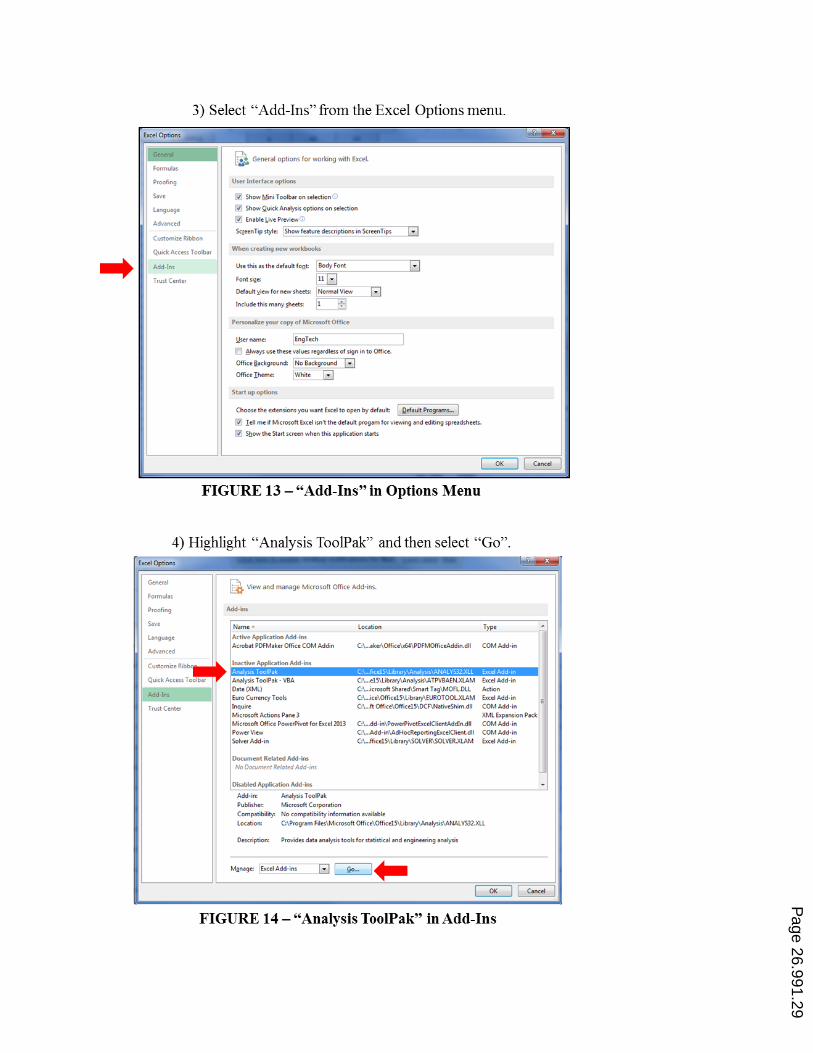
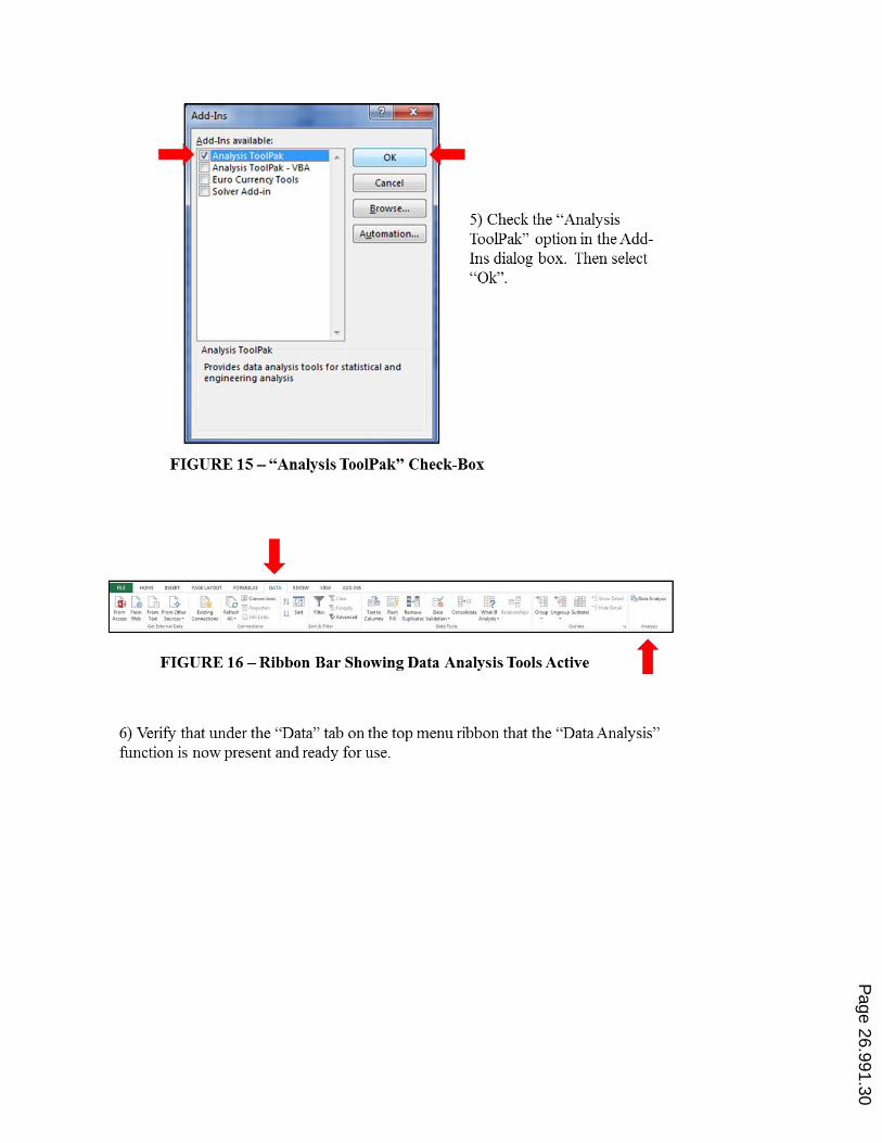
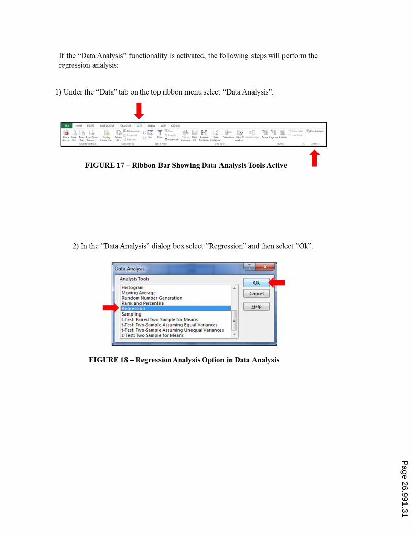
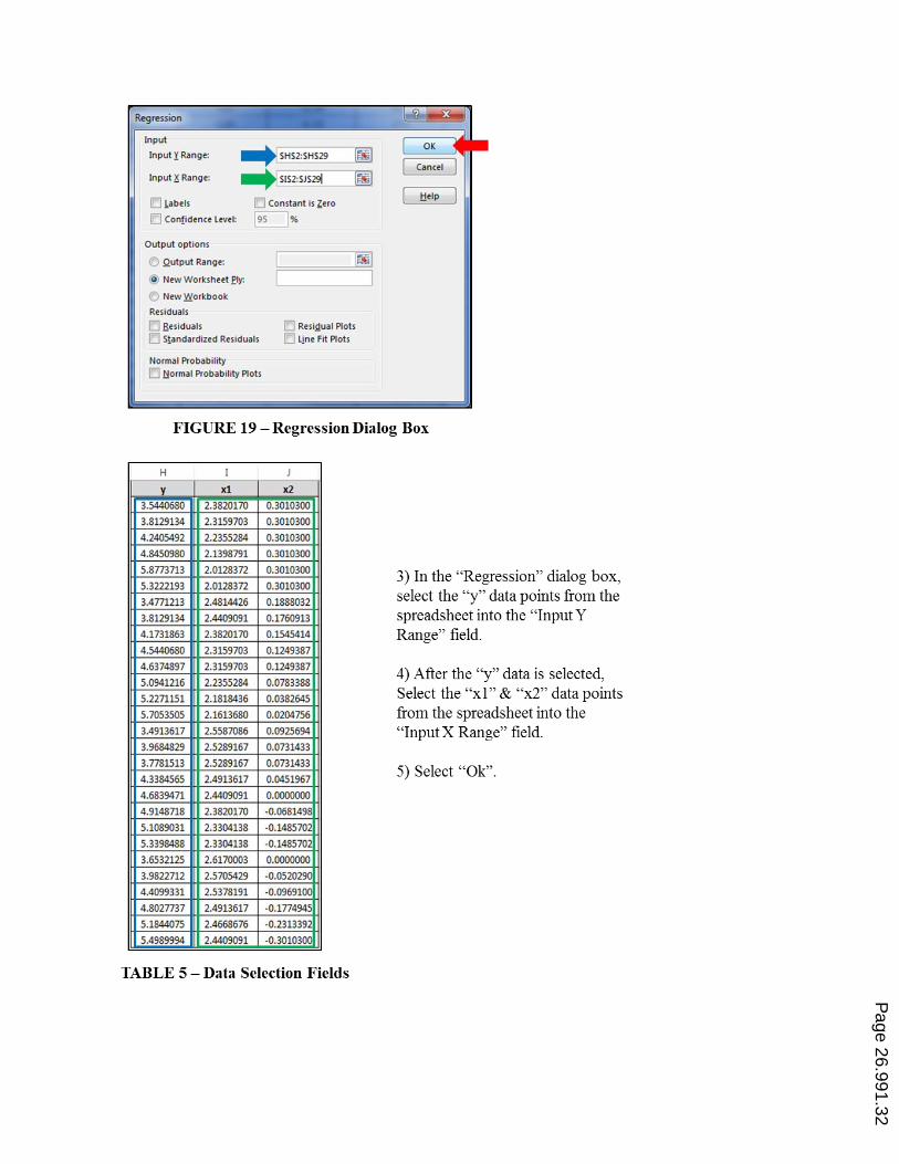
Prior to performing the regression analysis, the appropriate analysis tools may need to
be added to the MS Excel ribbon. The “Analysis ToolPak” will need to be activated to
access the required functionality.
The following steps will illustrate this process:
Page 26.991.28
Page 26.991.29
Page 26.991.30
Page 26.991.31
Page 26.991.32
Page 26.991.33
Page 26.991.34
Page 26.991.35

Bibliography:
1 Microsoft Website, http://news.microsoft.com/bythenumbers/index.html, Referenced January 17, 2015
2 Beer, Johnson, et al., Mechanics of Materials, 6th ed., McGraw-Hill, 2012, pp. 439-445
3 Mott, Robert, Machine Elements in Mechanical Design, 5th ed., Pearson, 2014, pp. 496-497
4 Cook, Young, Advanced Mechanics of Materials, 1st ed. Prentice-Hall, 1985, pp. 92-96
5 Hibbeler, R.C., Engineering Mechanics: Dynamics, 12th ed. Prentice-Hall, 2010, pp. 5-40
6 White, Frank, Fluid Mechanics, 7th ed. McGraw-Hill, 2008, 495-496
7 Dowling, Norman, Mechanical Behavior of Materials, 2nd ed. Prentice-Hall, 1999, pp. 452-458
Page 26.991.36