integrated scheduling and information support system for
TRANSCRIPT

University of South FloridaScholar Commons
Graduate Theses and Dissertations Graduate School
3-25-2005
Integrated Scheduling and Information SupportSystem for Transit Maintenance DepartmentsPaula Andrea Lopez AlvaradoUniversity of South Florida
Follow this and additional works at: https://scholarcommons.usf.edu/etd
Part of the American Studies Commons
This Thesis is brought to you for free and open access by the Graduate School at Scholar Commons. It has been accepted for inclusion in GraduateTheses and Dissertations by an authorized administrator of Scholar Commons. For more information, please contact [email protected].
Scholar Commons CitationLopez Alvarado, Paula Andrea, "Integrated Scheduling and Information Support System for Transit Maintenance Departments"(2005). Graduate Theses and Dissertations.https://scholarcommons.usf.edu/etd/746

Integrated Scheduling and Information Support System for Transit Maintenance
Departments
by
Paula Andrea Lopez-Alvarado
A thesis submitted in partial fulfillmentof the requirements for the degree of
Master of Science in Engineering ManagementDepartment of Industrial and Management Systems
College of EngineeringUniversity of South Florida
Major Professor: Grisselle Centeno, Ph.D.Paul McCright, Ph.D.
Jose Zayas-Castro, Ph.D.
Date of Approval:March 25, 2005
Keywords: allocation of resources; time standards, process standards, bus transit, forecasting.
Copyright 2005, Paula Andrea Lopez-Alvarado

ii
DEDICATION
To my family

iii
ACKNOWLEDGEMENTS
I would like to thank Dr. Grisselle Centeno for her guidance, support, dedication, and motivation throughout these years of study. Her commitment has been decisive to the success of this journey.
I would also like to thank Dr. Jose Luis Zayas-Castro and Dr. Paul McCright for their thoughtful reviews and advice during this thesis development.
Finally, I would like to express my gratitude and love to my family who has been always my support and has always given me confidence to accomplish my goals.

i
TABLE OF CONTENTS
LIST OF TABLES ........................................................................................................ iiiLIST OF FIGURES........................................................................................................ivABSTRACT....................................................................................................................vCHAPTER 1 INTRODUCTION......................................................................................1
1.1 Scheduling Situation in Transit Maintenance Facilities...................................51.2 Proposed Scheduling Situation in Transit Maintenance Facilities....................61.3 Thesis Organization........................................................................................8
CHAPTER 2 LITERATURE REVIEW...........................................................................92.1 Time / Work Standards...................................................................................92.2 Transportation Scheduling............................................................................112.3 Maintenance Forecasting..............................................................................132.4 Performance Measurements..........................................................................132.5 Information Systems ....................................................................................172.6 Other Transportation Applications................................................................192.7 Summary......................................................................................................20
CHAPTER 3 PROBLEM STATEMENT.......................................................................233.1 Motivation....................................................................................................243.2 Managerial Motivation .................................................................................253.3 Research Objectives .....................................................................................26
CHAPTER 4 TIME / WORK STANDARDS DEVELOPMENT ...................................274. 1 Task Identification.......................................................................................274.2 Pilot Readings ..............................................................................................294.3 Task Detailing..............................................................................................304.4 Observations ................................................................................................324.5 Preliminary Standards Development.............................................................334.6 Analysis .......................................................................................................344.7 Proposed Time Standard...............................................................................364.8 Implementation/Verification of Proposed Time Standards ............................37
CHAPTER 5 DEMAND FORECASTING MODEL DEVELOPMENT ........................405.1 Forecasting Model Applied to Failure Incidences .........................................49
CHAPTER 6 THE SCHEDULING MODEL.................................................................536.1 Basic Model .................................................................................................536.2 Extended Model ...........................................................................................556.3 Heuristic Approach ......................................................................................576.4 Model Testing and Results ...........................................................................596.5 Productivity Measurement............................................................................65
CHAPTER 7 THE INTEGRATED MAINTENANCE INFORMATION SYSTEM.......67

ii
7.1 Database Specifications................................................................................677.1.1 Database tables ..............................................................................697.1.2 Database input forms .....................................................................71
7.2 Application ..................................................................................................73CHAPTER 8 CONCLUSIONS AND FUTURE RESEARCH .......................................78
8.1 Conclusions..................................................................................................788.2 Future Research............................................................................................80
REFERENCES..............................................................................................................81APPENDICES...............................................................................................................84
Appendix 1: Algorithm – Heuristic Approach ...................................................85

iii
LIST OF TABLES
Table 1: Summary of Authors and Studies Related to IMIS Research ..........................22Table 2: Results for Brake Repair and Preventive Maintenance ...................................39Table 3: Characteristics of Forecasting Models ............................................................41Table 4: Forecasting Methods Applied to RCs of Brakes Repair System......................44Table 5: Test of Hypothesis for the Variances of MA and SES ....................................47Table 6: t-Test: Paired Two Sample for Means (A/C Jobs)...........................................48Table 7: t-Test: Paired Two Sample for Means (MA)...................................................49Table 8: Possible Monthly Outcomes of Engine Repairs for Year 2005........................50Table 9: Performance Rating for Technician i on Job k................................................60Table 10: Outcomes of the Objective Function for Scenario 1........................................60Table 11: Outcomes for Constraint 7 – Scenario 1 .........................................................61Table 12: Outcomes of the Objective Function for Scenario 2........................................61Table 13: Outcomes for Constraint 7 – Scenario 2 .........................................................62Table 14: Outcomes of the Objective Function for Scenario 3........................................63Table 15: Outcomes for Constraint 7 – Scenario 3 .........................................................63Table 16: Outcomes of the Objective Function for Scenario 4........................................64Table 17: Outcomes for Constraint 7 – Scenario 4 .........................................................64Table 18: Percentage of Utilization per Bay – Current Scheduling .................................66Table 19: Table System .................................................................................................70Table 20: Table Vehicle.................................................................................................70Table 21: Table Daily Schedule .....................................................................................71

iv
LIST OF FIGURES
Figure 1: Net Population Change for States from 1993 to 2020......................................1Figure 2: Model of the Integrated Maintenance Information System (IMIS)...................3Figure 3: Work Scheduling Model Interaction ...............................................................5Figure 4: Current Scheduling System.............................................................................6Figure 5: Proposed Scheduling System ..........................................................................7Figure 6: Relationship Between Maintenance, Reliability and System Performance Models ..........................................................................................................14Figure 7: Flowchart to Identify Key Issues Associated with MPM ...............................16Figure 8: Typical Transit System (Etschmaier and Anagnostopoulos, 1984) ................18Figure 9: Integrated Maintenance Information System (IMIS) .....................................24Figure 10: Repair Time Standard (RTS) Development Cycle .........................................28Figure 11: Time Study Worksheet .................................................................................31Figure 12: Processes for Preventive Maintenance ..........................................................35Figure 13: Forecasting Methods Evaluation ...................................................................42Figure 14: Actual Data vs. MA and SES for Brakes.......................................................45Figure 15: RCs vs. Forecasting Models for A/C System.................................................46Figure 16: RCs (02-04) vs. Forecast with MA for Engine System..................................51Figure 17: Productivity Improvement – Brake Jobs........................................................66Figure 18: Table Employee – Fields, Data Types and Description..................................68Figure 19: Table-Relationship Diagram .........................................................................69Figure 20: Information Stored in Table “Employee” ......................................................69Figure 21: Employee Data Form....................................................................................72Figure 22: Daily Scheduling Form.................................................................................72Figure 23: Work Order Form .........................................................................................73Figure 24: Graphical Report for Performance Level (Brake and PM Jobs) .....................75Figure 25: Scenarios of Scheduling Based on Standard Times .......................................76Figure 26: Database Input Form – Daily Scheduling......................................................77Figure 27: List of Technicians Available for a Morning Shift Scheduling ......................77

v
INTEGRATED SCHEDULING AND INFORMATION SUPPORT SYSTEM FOR
TRANSIT MAINTENANCE DEPARTMENTS
Paula Andrea Lopez-Alvarado
ABSTRACT
The projected increase of population in the United States and particularly in the
state of Florida shows a clear need of improvement in mass transportation systems. To
provide outstanding service to rides, well maintained fleet that ensures safety for riders
and other people on the streets is imperative.
This research presents an information support system that assists maintenance
managers to review and analyze data and evaluate alternatives in order to make better
decisions that maximize efficiency in operations at transportation organizations. A
system that consists of a mathematical scheduling model that interacts with a forecasting
model and repair time standards has been designed to allocate resources in maintenance
departments. The output from the mathematical models provides the data required for the
database to work.
Although the literature presents several studies in the field of maintenance
scheduling and time standards, it stops short in combining these approaches. In this
research, mathematical methods are used to forecast repair jobs occurrence to react to
increments in service demand. Furthermore, an integer programming scheduling model

vi
that uses the data from both, the developed time standards and the forecasting model is
presented. The information resulting from the models is entered to a database to create
the information support system for transit organizations. The database gives the
scenarios that facilitate optimizing the allocation of jobs in the facility and determines the
best workforce for each required task.
Information was obtained from observations at three transit facilities in the
Central Florida area; the model developed is tested in their scenario by using historical
data of the maintenance jobs currently performed. Outputs obtained from testing have
demonstrated reduction of operational costs, increased bus reliability, and efficiency in
the tasks executed. Therefore, the present study aggregates value to transit organizations.

1
CHAPTER 1
INTRODUCTION
According to the United States Census Bureau, the population is estimated to
increase in high proportions in the near future. California reports to be the most heavily
populated State and the one that expects to grow in the highest proportion. Texas and
Florida are expected to be the next biggest gainers. Florida is projected to add 2 million
immigrants and after California and Texas should see a net gain of nearly 4 million from
other States. www.census.gov/population/www/pop-profile/stproj.html Figure 1 presents
the net population change for States gaining at least 1 million persons from 1993 to 2020.
Figure 1: Net Population Change for States from 1993 to 2020

2
As it is seen in figure 1, there is a steady increase in population forecasted for the
upcoming years that makes necessary improvement in the public transportation service.
According to the Hillsborough County Metropolitan Planning Organization (MPO), by
the year 2025, the population in Hillsborough County is expected to increase by 41% and
the employment in the area is forecasted to increase by around 62%. Along with this, the
total Vehicle Miles Traveled (VMT) is expected to increase by 52%. However, the
planned roadway capacity is not expected to increase as much as the demand. These
increments of demand force transit companies to develop better services since public
transit in general represents an important factor of growing as a way to improve mobility
http://www.hillsboroughmpo.org/about/index.htm.
Excellence in service starts from the base of public transportation organizations
where maintenance departments play an important role. High demand of service results
in a need for providing efficient and effective maintenance to the fleet. The statistics
presented and their implications in efficient maintenance practices are motivators for the
development of better systems that help managers improving productivity.
In this research, maintenance information from public transit facilities is explored
using analytical tools to develop an integrated maintenance information system. The
system developed is intended to assist managers in the optimization of maintenance
operations, therefore efficient and effective service to the fleet.
Figure 2 illustrates how the study generates a coordinated system that processes
the relevant information and supports the maintenance facility decisions while giving
administrative alternatives to maintenance managers.

3
Figure 2: Model of the Integrated Maintenance Information System (IMIS)
The system inputs are grouped by factors associated with the transit environment
that affects maintenance departments. All the factors should be connected to give better
service to the customers and reduce potential damage to the environment.
Operational factors: represent the basic information that the system requires to
work including data about technicians, fleet, and maintenance processes.
Environment or external factors: correspond to the factors that drive the demand
of maintenance jobs.
Different tools can be used to develop the maintenance scheduling and
information system. The specific methods used for this research and complete
descriptions of them are presented in chapter 4:
Work analysis: tools such as time studies and work design can be used to
determine work efficiency in the facility. These tools play an important role in
IntegratedMaintenanceInformation
System
• People (Technicians)
• Fleet
• Maintenance processes
• People (population)
• Type of public transportation
• Demand
• Time standards
• Work design (facility layout)
• Forecasting methods (static methods, adaptive forecasting, moving average)
• Optimization methods (goal programming network flows, linear programming)
• Databases and Spreadsheets
Tools
Input(information about…)
Output
Technicians’ performance Fleet maintenance history Facility resource allocation Maintenance standard processes
Ope
rati
onal
Ext
erna
l

4
the standardization of repair fleet processes as well as in the measurement of
workforce performance.
Forecasting methods: depending upon the variability of the factors that influence
the maintenance demand different methods of forecasting maintenance
occurrences are used.
Optimization: a linear programming model is used to determine the best
allocation of resources in the shop.
Software tools: databases and spreadsheets are used to develop the interface
between the model and the end users of the information system.
Figure 3 presents how the proposed work scheduling model could impact the
allocation of transit maintenance resources to increase efficiency and effectiveness in the
facility. The inputs for this model are the forecasted demand of bus maintenance, the
workforce availability, the physical capacity of the facility and the repair time standards
developed. The work scheduling will assist managers in how to allocate their resources
and to better plan training sessions that will positively impact the functioning of the
facility.

5
Figure 3: Work Scheduling Model Interaction
1.1 Scheduling Situation in Transit Maintenance Facilities
The scheduling system currently in place at transit facilities is shown in Figure 4.
The flow shows that for the preventive maintenance (PM) case, the buses are sorted
according to their daily mileage, information that serves as the base for maintenance
scheduling. Additionally, if the buses need to be repaired they have to be assigned to an
empty bay. The main constraint for maintenance scheduling is bay availability in the
facility; a factor that prevents the prompt execution of more jobs due to the facilities’
physical space limitations. After the buses are pulled out from the route, technicians are
scheduled, based on the type of maintenance tasks to be performed on the particular bus.
If there are no technicians available the bus is parked idle.
Work Scheduling
Model
• Workforce availability
• Capacity of the facility
• Maintenance demand
Influence
Time standardization of maintenance jobs
Facilitates
• High quality of maintenance processes
• Increasing of customer satisfactionGenerates
Generates
Training programsFacilitates
Workforce efficiency & effectivenessManagement of technological changes
Facilitate
Tools Optimization Forecasting Work design Time studies Six sigma Human relations
Forecasting of maintenance demand

6
Figure 4: Current Scheduling System
1.2 Proposed Scheduling Situation in Transit Maintenance Facilities
The proposed scheduling model is similar to the current system but takes
advantage of the repair time standards study to allocate more buses for maintenance in a
shift, and to assign the best qualified technician to the job (see figure 5). Here, depending
upon the work load and the time available, either one or two jobs are assigned to a bay
during one single shift, which maximizes the resource utilization of the maintenance
facilities.
Bus needs maintenance
Technician is assigned to a bus maintenance job
Technician available?
Bay available?
Bus is assigned to a bayBus is parked
Yes
YesNo
No

7
Figure 5: Proposed Scheduling System
Repair standard time is a factor that could constrain the number of jobs to be
assigned to a particular bay as well as to a particular technician. If a job could be
completed in half a shift or less, another bus could be assigned to the bay for additional
repair or procedures. Likewise, if the job’s standard time is higher than the time
available in the bay, the bus is assigned to a new bay. A bus is parked only if there is no
technician available to perform the required job. Since the model attempts to improve
productivity, technicians could be assigned to more than one job during the day
depending upon the type of job to be performed.
Bus is scheduled for maintenance
Totaltime = Totaltime -Jobtime
Technician available?
Bay available?
Bus is assigned to a bay
Bus is parked
Yes
YesNo
No
Type of maintenance
Job time <= totaltime?
Assigns technician with highest performance level to the maintenance job
Yes
No

8
Efficiency is increased when the best allocation of maintenance jobs is made and
fewer buses are parked to wait for service. Similarly, quality is improved by using
standard repair processes and constantly following up with technicians’ performance.
Finally, training is better assessed for this process and it is facilitated by using the time
and process standardization which promotes better execution of the jobs.
1.3 Thesis Organization
This thesis have been organized as follows: Chapter 2 identifies the most
significant studies related to transit systems. Chapter 3 describes the problem statement
and the motivation for the research. Chapters 4, 5 and 6 present the time standards, the
forecasting model, and the scheduling model developments and evaluations. Chapter 7
includes the integrated maintenance information system and application. Finally, Chapter
8 presents the conclusions and recommendations of the study, including future research
opportunities.

9
CHAPTER 2
LITERATURE REVIEW
A vital issue for safely operating transit systems is the appropriate maintenance of
vehicles and equipment. According to the Federal Transit Administration (2001) safe
vehicles prevent accidents and reduce risks to the driver, passengers, or other vehicles on
the road. Maintenance practices must be regularly addressed to ensure that there is no
unsafe vehicle on the road.
To improve management of transit maintenance departments, tools such as work
standards, work scheduling, forecasting methods and management information systems
could be utilized. The following sections summarize the work conducted in these areas,
and discuss the impact in transit maintenance.
2.1 Time / Work Standards
Different studies have been developed to establish fleet maintenance time
standards. Most studies have been built based on historical data and time estimations.
Their main objective is to determine, and further control, the workforce performance in
transit maintenance facilities.
Inaba (1984) reviews the use of work standards for transit bus maintenance.
Different agencies from the U.S. and Canada were surveyed to determine if they used
work standards and to what extent. According to this study, most programs had standards
10
for inspection, PM, corrective maintenance and unit repair. The least attention was given
to troubleshooting. The study also showed that work standards were used to identify
problem areas, establish manual work schedules and to monitor personnel performance.
The work standards programs of the Chicago Transit Authority and of Metro Transit of
Seattle had the most extensive documentation. In this study, historical information and
the generic steps to develop work-motion studies were used to standardize maintenance
processes for transit fleet.
Purdy (1990) presents a methodology that uses historical data from an
information system to establish preliminary work standards for division performed
maintenance. The research objectives were centered on three aspects: to identify
components that account for significant consumption of maintenance labor; to develop
tools to increase workforce productivity; and to provide guidelines for daily and annual
maintenance planning. Once again, it was found that most of the standards used in transit
facilities are based on estimations from historical information.
Schiavone (1997) summarizes the work standard approaches employed by four
transit agencies and a private company. He also presents the different methods used to
monitor maintenance performance. The report reveals that many transit agencies expect
maintenance employees to adhere to written procedures when performing routine tasks.
Many agencies use original equipment manufacturers (OEM) service manuals as the base
to establish their own work procedures and time standards. Other agencies have based
standards on a combination of OEM and historical repairs rather than using on-site
analytical methods.

11
Venezia (2004) summarizes information from transit facilities that have
developed successful productivity improvement programs in order to gain insight into
those properties’ practices and procedures. The study presents data from transit
companies that vary in terms of size, union, affiliation, and operating conditions. The
results showed that many agencies use time standards as a guide to monitor employees
and some others use them as a goal. Once again it was shown that most agencies use
OEM, historical data and estimations to develop the standards.
As part of this study, a systematic method for determining repair time standards
for transit buses is developed. The methodology analyses the flow observed on-site in
three maintenance facilities to determine best maintenance practices. Furthermore, the
current practices are analyzed and compared with the written procedures used at each
participant facility. The analysis through various facilities and written procedures help in
the generation of feasible and adaptable standards for transit facilities across the state and
the nation.
2.2 Transportation Scheduling
Effective scheduling is necessary to optimize production lines and services.
Martin-Vega (1981) demonstrated that the principle behind shortest processing time
(SPT) sequencing could be applied to job shop bus maintenance. The use of SPT resulted
in more jobs completed in less time and reduced waiting average time, which translates to
a reduction in work-in-process inventory.

12
In public transit maintenance, the optimization of repair and inspection service
represents minimization in costs and maximization of fleet utilization. Scheduling
practices then serve as an efficient method to better utilize available resources.
Haghani and Shafahi (2001) developed a bus maintenance scheduling model to
design daily inspections and maintenance schedules. The model maximizes the
utilization of the maintenance resources while reducing the time that buses are idle when
pulled from daily activities. This approach was focused on preventive maintenance (PM)
scheduling, and presented both a mathematical formulation and a solution procedure.
The objective function has two components: The first is maximizing a weighted
total vehicle maintenance hours (maintenance utility) for the buses that are pulled for
maintenance when idle, and the second is minimizing the weighted total number of
maintenance hours for the buses that are pulled out of their scheduled service for
inspection.
Although the purpose of work maintenance scheduling is to ensure that the
maintenance scheduling system runs efficiently over a period of time, other factors
should be taken into account in order to implement an effective and efficient maintenance
service system. Minimization of the operational costs, maximization of resources
utilization, and need of high quality maintenance practices emerge as challenges for the
public transit maintenance managers.
The research approach maximizes the number of buses served during a shift while
optimizing the allocation of the resources according to the repair time standards
established in the transit maintenance facilities. It does not only consider preventive
maintenance (PM) jobs, but also repair jobs and road calls (RC). This model assumes

13
that there is always availability of parts; otherwise, the jobs need to be re-scheduled when
the parts are on hand.
2.3 Maintenance Forecasting
Transit facilities keep track of the occurrences of every job to generate statistics of
the jobs performed each year. However, forecasting jobs based on previous occurrence is
rarely done. Maintenance managers and supervisors are able to prognosticate and
perhaps, schedule inspections due dates. Jobs such as PMs, engine and/or transmission
repairs are planned based on mileage intervals, hours operated or fuel used.
No studies have been found related to transit maintenance jobs forecasting or
using any scientific formulation to predict repair jobs occurrence. The study presented
uses historical information as well as the traditional methods to develop mathematical
forecasting approaches for maintenance jobs in transit facilities. It assists with the
counting of coming inspections and also helps managers with the prognostication of
possible break down occurrences.
2.4 Performance Measurements
When developing organizational or departmental improvements, it is important to
conduct the post-implementation evaluation to assess the changes being done and to
evaluate improvements. Applying quality measurements is very important after
developing time standards for the various processes. They are necessary to keep track of
the transit fleet maintenance and the technician’s task accomplishment.

14
Guenthner and Sinha (1983) provided a method to link a maintenance model, a
reliability model, and a performance evaluation model to evaluate the relation between
the system operating performance and maintenance policy. The maintenance model
provides the level of dependability as a function of the number of spare buses and the
number of mechanics; the reliability model uses the dependability value to determine
average passenger waiting times, based on the theory that undependable service will
cause long waiting times, and the performance evaluation model quantifies the effect of
waiting times on ridership and examines the overall system performance. The
relationship between the three models presented in the study is shown in the Figure 6.
Figure 6: Relationship Between Maintenance, Reliability and System Performance
Models
According to Inaba (1984), one of the applications of work standardization is to
assure better maintenance scheduling based on individual judgments since it is easier to
determine how long it should take for a particular technician to accomplish a job. For
Vehicle Maintenance
Number of Spare Buses
Number of Mechanics
MaintenanceModel
ReliabilityModel
PerformanceEvaluation
Model
Route Length Headway
Passenger Waiting Time
Operating Data
Ridership and System Performance

15
some of the agencies where standards were implemented, a system was also developed to
compare the actual performance versus the standards.
List and Lowen (1987) report the results of a survey regarding bus maintenance
performance indicators. They observe that RCs are the most important performance
indicator followed by a turn inward to search for cause (i.e., drivetrain performance), and
to monitor labor and monetary productivity. They also state that differences in
managerial point of view appear to stand in the way of an agreement on a single list of
indicators and their ranking.
As List and Lowen noticed, not all of the maintenance jobs and technicians’
performance were always used to establish performance measurements. Computerized
information systems emerged as a powerful tool to record any variability in technicians
working and in the fleet operation. The integrated maintenance information system
intends to relate data from maintenance departments in order to develop accurate and
comprehensible performance indicators.
Schiavone (1997) summarizes the different methods that transit agencies use to
monitor maintenance performance and illustrates how performance measurements are
used to help shape maintenance programs. He identifies the key issues in elements of bus
maintenance performance. Figure 7 shows the flowchart used by Schiavone to identify
the key issues associated with maintenance performance monitoring (MPM) which
include management philosophy, employee productivity, equipment performance and
cost. The driven force of three factors on top is people. It is imperative for people to
perform properly. Management philosophy refers to the role that managers play when
motivating and training people to perform competitively. The employee productivity

16
bases its rating on the way in which technicians perform their jobs. For this, time
standards are cross-checked with their performance. Equipment performance will highly
depend on how people perform. Better maintenance practices and good scheduling
practices will result in better equipment performance and fewer RCs. Finally, these three
approaches are closely related with cost since their accomplishment is translated into cost
reductions.
Figure 7: Flowchart to Identify Key Issues Associated with MPM
According to Shiavone’s report, agencies usually develop their own maintenance
performance monitoring program based on OEM service manuals, work orders and the
Federal Transit Administration (FTA) National Transit Database (NTD). The study was
conducted on four transit agencies and one private truck company.
Performance indicators are intended to reach for excellence. Therefore, transit
maintenance departments should construct their own performance programs based on
actual data and by applying quality standards. In this thesis, the time and process
MANAGEMENTPHILOSOPHY
• Setting an example• Degree of oversight• Employees specialization• Incentives/Discipline• Communication
EQUIPMENTPERFORMANCE
• Pullouts• Road calls• PM intervals• Standardization• Driver involvement• Customer acceptance
COST• Cost reports based on monitoring• Change procedures based on report results• Determination of how costs reductions were achieved
EMPLOYEEPRODUCTIVITY
• Work procedures• Time monitoring• Faulty workmanship• Troubleshooting• Training

17
standards developed for three transit facilities is utilized to determine better flows that
facilitate superior maintenance practices. Furthermore, it develops an IMIS to track and
report technician’s performance compared with the time standards established.
According to Venezia (2004), the most significant performance indicators are
number of RCs, premature failures, pullouts, scheduled work compared with unscheduled
work, repeated failures, and inspections completed on schedule. Although these practices
are recognized by transit agencies, no systematic approach was found to accurately
monitor these performance indicators.
The research presented in this thesis develops a scheduling model based on time
standards. It can optimize resource allocation and assures reliable maintenance
processes. These measurements would help to demonstrate the impact of processes
standardization on RCs and the minimization of maintenance costs. After implementing
the scheduling model based on the forecasted maintenance demand and using repair time
standards as time constraints, the system needs to be evaluated. This approach intends to
improve the transit maintenance system practice by preparing departments with tools that
facilitate the fast response to unexpected situations that consume time from regular and
scheduled tasks. This will reduce the number of unexpected break downs that affect the
public transit service image and add operational costs to the companies.
2.5 Information Systems
Information Systems are widely used by management in areas such as allocation,
distribution, scheduling, decision/risk analysis, and process management and control.
Developers must use quantitative techniques such as mathematical programming,

18
optimization models, statistical patterns, and forecasting techniques in order to exploit the
IS and to facilitate the modeling of real environments.
In the public transportation field, diverse maintenance management models have
been developed in order to keep track of relevant information. Managers use this
information to manually schedule jobs and workforce. This system generates feasible
solutions that typically are not optimal.
Etschmaier and Anagnostopoulos (1984) presented a typical transit system where
three major functional elements support the entire system. However, maintenance
departments are commonly isolated from the system and wrongly seen as the department
that only increases costs to the company. Figure 8 shows how maintenance must be
considered along with marketing and operations as major elements in a transit system.
Figure 8: Typical Transit System (Etschmaier and Anagnostopoulos, 1984)
To change how people perceive transit maintenance departments, it is necessary to
develop tools that help managers in attaining high productivity and moving the
maintenance departments closer to the strategies of the company.
System
Marketing
Maintenance
Operations

19
Boldt (2000) documents the state of the practice in management information
systems (MIS) and compares communication technologies versus a contemporary
background of business practice. The synthesis is organized into the basic architectural
pieces that constitute an IT plan to provide the essential framework for the planning
process. Additionally, he documents organizational issues and policies as well as market
trends affecting the deployment of MIS technology.
The results have shown that the areas mainly evaluated by organizations are
administration, planning and operations. As it is presented, although maintenance
departments play an important role in organizations, they are not frequently considered as
a relevant part of the company. However, transit organizations rely on maintenance
departments to keep vehicles in safe conditions and to give outstanding service to the
riders. Maintenance information systems should also be taken as an important part for
companies to improve operations.
2.6 Other Transportation Applications
This section discusses maintenance scheduling application and optimization
models developed for aircraft and railcar.
Hall (1998) developed a set of models to evaluate and compare the efficiency of
alternative layouts for railcar maintenance. The model assesses two rules for assigning
jobs to shop stalls, one is based on utilizing stalls in tandem with inserted idle time, and
the other one without inserted idle time. In one of the cases modeled, jobs are selected
for maintenance on the basis of repair and car characteristics. The cars are divided into
maintenance classes represented by PM or repairs. It can be noted that when multiple
20
tracks are available for shop lay-up, tracks can be assigned different classes, further
reducing the expected number of moves. The models presented by Hall show the
importance of facility design combined with scheduling as driven factors of efficiency in
maintenance efficiency. Learning from the railcar scheduling and layout design
experience, different approaches can be used to model the scheduling approach for bus
maintenance, based on facility design. Shifts and bays can be arranged according to the
demand needs to accomplish effective maintenance schedules.
Sriram and Haghani (2001) presented a formulation and a heuristic approach for
aircraft maintenance scheduling and re-assignment. The model objective is to minimize
the maintenance cost and other costs incurred for the re-assignment of aircraft to the
flight segments. In this case, the aircraft is assigned to flights before maintenance is
scheduled. These factors play an important role to determine which aircraft should fly
which segment and when and where each aircraft should undergo the different levels of
maintenance inspection. Only two types of PM are considered and unexpected
requirements are not considered either.
As in the case of bus maintenance scheduling, the approach only considers PM
tasks to allocate resources. Moreover, the model takes into consideration a short horizon
of time to assign the aircraft to maintenance jobs.
2.7 Summary
In this chapter, the literature that is relevant to the presented research in the areas
of time standards, forecasting, maintenance scheduling, and management information
systems have been reviewed both from a methodological perspective and from a practical

21
perspective. Since most of the related work is outdated, the presented review has
concentrated on current practices and the fundaments required for solving the problem of
interest. Table 1 complements the written discussion by summarizing the models
encountered in the literature in the area of transportation maintenance systems. It is
manifested that different studies can be potentially functional for maintenance
departments but an integration of them is still needed.
The last item presented in the list corresponds to the proposed research and
reflects how this study combines and updates approaches from the areas reviewed.

22
Table 1: Summary of Authors and Studies Related to IMIS Research
Author Year Title
Tim
e/w
ork
Stan
dard
s
Tra
nspo
rtat
ion
Sche
duli
ng
Mai
nten
ance
Fo
reca
stin
g
Perf
orm
ance
M
easu
rem
ents
Info
rmat
ion
Syst
ems
Tra
nsit
App
licat
ions
Oth
er
Tra
nspo
rtat
ion
App
licat
ions
Martin-Vega, L.A. 1981SPT, Data Analysis, and a Bit of Common Sense in Bus Maintenance Operations: A Case Study
Guethner, R; Sinha, K 1983Maintenance, Schedule Reliability and Transit System Performance
Inaba, K 1984 Allocation of Time for Transit Bus Maintenance Functions
Etschmaier, M; Anagnostopoulos, G 1984 Systems Approach to Transit Bus Maintenance
List, G; Lowen, M 1987Bus Maintenance Performance Indicators: Historical Development and Current Practice
Purdy, J 1990 Work Standards: Their Use and Development Using a MIS
Schiavone, J. 1997TCRP Synthesis of Transit Practice 22: Monitoring Bus Maintenance Performance.
Hall, R.W. 1998Scheduling and Facility Design for Transit Railcar Maintenance
Boldt. R. 2000TCRP Synthesis of Transit Practice 35: Information Technology Update for Transit
Haghani, A; Shafahi, Y 2001Bus Maintenance Systems and Maintenance Scheduling: Model Formulations and solutions
Sriram, Ch., Haghani, A. 2001An Optimization Model for Aircraft Maintenance Scheduling and Re-assignment
Venezia, F. 2004TCRP Synthesis of Transit Practice 54: Maintenance Productivity Practices
21
Lopez, P., Centeno, G. 2004Integrated Maintenance Information System for Transit Organizations

23
CHAPTER 3
PROBLEM STATEMENT
Although the literature presents several studies in the field of maintenance
scheduling and time standards, it stops short in combining these approaches. Time
standards have been developed to increase efficiency in maintenance processes. On the
other hand, scheduling models have been developed also to improve efficiency based on
service waiting times. However, to the best of our knowledge no study that improves
efficiency in transit maintenance operations by scheduling jobs based on time standards
and estimations of demand was found.
This research integrates forecasting methods that model the behavior of the repair
demand in transit maintenance departments. The results are used as input to a
mathematical model that schedules resources such as technicians and bays in
maintenance shops. The assignment is based on the importance of the repair type.
Furthermore, the system uses repair time standards results to allocate as many jobs as
possible to a shift. The use of repair standard times is fundamental when allocating the
most experienced technicians. A database that integrates information from those systems
is developed. It contains feasible, comprehensible, and useful reports to maintenance
managers and supervisors. Figure 9 shows how the output from the models will interact
with the database.

24
Figure 9: Integrated Maintenance Information System (IMIS)
3.1 Motivation
As it was explained in Chapter 2, several studies have been conducted in the field
of maintenance in public transportation including scheduling, planning, process
optimization and policies. However, most studies have been done over 20 years ago and
they mostly show solutions that stand by themselves without considering the other
planning components for maintenance management.
According to the Transit 2020 developed by the Florida Department of
Transportation (FDOT) in collaboration with state and local government agencies, transit
providers, community leaders and the general public: “Transportation’s needs into the
21st Century cannot be met with highways alone. Improved public transportation is
crucial to expanding travel choices.”

25
(http://www.dot.state.fl.us/transit/Pages/transit2020plan.htm) This quotation emphasizes
the need for improvement in public transit organizations in order to conserve a reliable
fleet, and to meet the increases in demand.
The future of urban transportation represents a challenge to maintenance
managers due to the foreseen high utilization of the fleet. Currently, the low demand of
urban transportation denotes relatively low problems for scheduling and technicians’
productivity. However, when demand increases the service should remain the same in
quality and accomplishment. Since maintenance shops cannot increase capacity every
time demand increases, a need for optimization is evident to compensate for high
amounts of work.
Having reliable maintenance information systems that efficiently keep the
information under control and supports managers when making decisions is a challenging
task. It is necessary to count on reliable systems that can manipulate and organize the
information related to the internal and external factors that may affect the functioning of
the transit facility and result in a consistent accomplishment of maintenance tasks.
3.2 Managerial Motivation
A successful organization is the result of the combination of efforts from the
various departments. Aligned administrative strategies could enhance the management of
the transit fleet maintenance, and as a result, improve service to the riders. Maintenance
departments play a fundamental role inside public transit companies. However, an
assessment of transit operations has revealed that they are usually segregated from the
rest of the company (Etschmaier, 1985). Typically, the main objective of these

26
departments is to maintain the fleet working safely and reliably without breakdowns. For
that reason, they should not be seen as a support element of the organization but as
another core unit that aggregates value to the transit facility.
Maintenance managers receive information from many different sources in the
organization which make their job tedious and difficult. IMIS is an information system
that provides desirable and friendly support through interfaces with appropriate format.
Moreover, managers will be able to test how different scheduling strategies would work
under various conditions to consider alternative plans.
3.3 Research Objectives
The objective of this research is to develop a scheduling model that allocates
resources at transit maintenance facilities, applying repair time standards developed and
technicians’ performance rating resulted from the standards. The scheduling satisfies an
input demand that comes either from current needs or from the forecasting of previous
demands. The development of a forecasting model that provides scenarios of demand
represents another objective of this thesis. Also, this research aims to integrate the
models in a database that works as a maintenance information system in order to assist
maintenance managers and supervisors in the optimization of resources.
This study applies the model developed to the environments of three transit facilities
in the state of Florida. A practical application of the models is presented to demonstrate
the relevance of the models and how the environment of a transit facility might be
impacted with the application of the proposed system.

27
CHAPTER 4
TIME / WORK STANDARDS DEVELOPMENT
Standardization of time and processes of maintenance tasks minimizes the time to
perform a job while improving process development. Standards are useful to determine
labor efficiency, to improve maintenance process control, and to improve facility layout.
In this study, nine steps have been proposed to establish repair time standards. These
steps cover the methodology shown in figure 10. The squares represent the steps
followed during the development of the methodology and the rounded boxes represent
the relevance of feedback of the people from the participating facilities.
The following section describes in detail the steps followed in the development of
the standards at four transit agencies. The methodology and application shown in this
section are extracted from Centeno, Chaudhary, Lopez, 2005.
4. 1 Task Identification
The first step is to identify the critical task or system to be studied; brakes, PM, or
engine and/or transmission replacement are examples of the maintenance systems. The
task(s) could be identified based on the priority for repair given at a transit facility.
Factors that could be considered to choose the task include frequency of service, or tasks
with failure components resulting in high risks or great loses.

28
Task Identification
Pilot Readings
Task Detailing
Observations
Preliminary Standard Development
Analysis
Propose Time Standard
Implementation /Verification of Proposed Standard
Information System Development
Input from Technicians
Input from Managers and Supervisors
Figure 10: Repair Time Standard (RTS) Development Cycle
With the agreement of a steering committee and other officials from Florida
Department of Transportation (FDOT), this study was initiated by identifying brake
repairs as the first task to be studied. Brake repair is one of the most important systems
in transit buses since failures on any of its components represent high safety risks and
liabilities. The second job studied was PM since periodical inspections enhances the
service life of the buses and increases safety. Additionally, PM is the task most
frequently performed at transit facilities.

29
4.2 Pilot Readings
This step allows the analysts to become familiar with the process being studied. The
development of the pilot readings required considerable experience on work
measurement analysis as well as good knowledge of the transit industry and bus
components. Initially, to understand the process of the jobs studied, various visits to the
participating facilities were necessary to record the total time required to perform a task.
The total time and procedure to complete the task was recorded for all the observations.
A typical concern from supervisors and technicians is the number of cycles that
will be observed before establishing the standards. If only a few observations are taken,
the standards could be questionable and/or erroneous. On the other hand, a big number
of observations is very costly and time consuming. For that reason, the formula
presented next is important to statistically determine the number of observations to be
taken to have results in a 95% confidence level (Niebel, and Freivalds, 2003).
2
,2/
xk
stn
Where: s is the standard deviation (time in minutes) from the pilot readings taken; t is the statistic computed using an (error) – typically set as 5 or 10% with n-1
degrees of freedom (υ); k is the accuracy which measures the closeness of the observed value to the true
value of the population – typically set as ± 5%; is the average value in minutes from the pilot readings taken.
The total number of cycles required for brakes job was computed to be 10.6
observations. To ensure the required accuracy, it was rounded up to 11 (Centeno, 2002).

30
2
,2/
xk
stn
116048.103.14950*1.0
303.4*44.11312
Similarly, various visits were made to the participating facilities to observe the
processes for the PM jobs. At the same time, related existent procedures and checklists
were collected to gain a better understanding of the processes. Later, this information is
used to facilitate the development of the proposed flow in PM activities. The total
number of observations required for PM was 13.55. This number was rounded up to 14
observations.
2
,2/
xk
stn =
2
14600*05.0
303.4*5.624
= 13.55 ~ 14 observations.
4.3 Task Detailing
With the completion of the pilot readings, the major processes within a task along with
the elements should be identified. Processes are the major components in a task; an
element is the smallest unit contained in a process. Oil change is an example of a process
within the PM task, and removing the filter is one of the elements in the oil change
process.
Each element should be studied and further classified according to the ASME
standard set of process chart symbols as an operation, transportation, storage, inspection
or delay (Niebel, and Freivalds, 2003). The definition and symbol of each classification
is as follows:

31
Operation: Activity that involves performing work on a part Transport: Movement from one place to another to perform an operation, part procurement or storageInspection: Observation of components to check conformity to the safety requirements
D Delay: Interruptions during the working process due to unnecessary (avoidable) or necessary (unavoidable) events. An avoidable delay is a pause in the productive work due to the technician non-work related causes, e.g., the technician is often out of his workplace for smoking. An unavoidable delay is an interruption of a normal process that is outside of the technician’s control, e.g., the technician has to wait for the oil to drain.
Storage: Event of accommodating parts on a different location
Classification of elements will provide valuable information of the workflow and
facilitate the identification of redundant elements. Figure 11 shows the standard form
developed to record the time taken to perform each element and provides a space to
classify it according to the type of activity.
Figure 11: Time Study Worksheet

32
During the course of taking the pilot readings, all the processes and elements for
each task were identified and studied carefully. The time of each element was as small as
3 to 4 seconds. For brakes, 10 processes and 260 elements were identified. For PM, 17
processes were identified. Similarly, nearly 300 elements were identified and classified.
4.4 Observations
When recording the observation the following criteria should be considered:
The observations should be taken objectively to minimize bias while describing
the elements and recording the times.
The technicians chosen should perform at a normal working pace. Some of the
observations may be repeated with the same technicians to check for consistency.
If possible, observations should be taken during different shifts during the day to
evaluate the impact of external factors such as surrounding light and weather.
Observations should be taken with no special arrangements and the emphasis
should be to develop standards for a typical environment. Moreover, special tools
or equipment infrequently available should not be employed when conducting the
study.
During the observations, the working pace of the technicians should be examined by the
analyst and categorized as normal, below normal (slow) or above normal (fast speed).
This practice is typically based on the experience and judgment of the analyst. Therefore,
the analyst should be adequately train to assign fair and impartial performance ratings
throughout the study. The time study worksheet previously illustrated (see Figure 11)

33
contains three columns to evaluate performance on each element. When the operator
performs at normal pace a 100% rate is assigned; below normal is accounted as 90% and
above normal as 110%. Note that a given operator may perform at different paces during
the completion of the tasks, thus, different percentages for the various elements could be
assigned. For the elements rated as above or below normal the normal time could be
obtained by multiplying the observed time to the rate.
4.5 Preliminary Standards Development
After completing taking the required observations, the workflow should be analyzed and
the best practices among facilities should be combined to develop a standardized flow.
The processes should be sequenced in such a way that redundant elements and elements
that cause delays are removed. The preliminary standards are determined by combining
all the valid observations and by taking the averages of the normal times for each
element.
The following factors should be considered when developing the preliminary standards:
Normal pace: Observed technicians should be encouraged and are expected to
work at a normal pace.
Worker habits: Habits that cause delays such as speaking to colleagues or
conferring with others while borrowing tools should be evaluated and restricted
without altering the actual processes. This will allow the construction of
standards that are feasible, realistic, and easily adopted by technicians.
Facility layout: To make the standards more robust and reusable, they should be
developed independently from the facility layout.

34
Actual readings: The preliminary standards should be based only on collected
data from the pilot readings and not on theoretical studies.
Developing preliminary standards for PM was relatively more challenging than
for brakes as it had many more independent components including inspection and
diagnosis. Brake repair is more systematic which makes sequencing one process over
other relatively more feasible than in PM. A modular approach that provides the
technician with flexibility to perform the process in any order preferred without altering
the total estimated time was adopted. Figure 12 shows the flow with the processes
developed for a 12,000 type of PM.
4.6 Analysis
All the observations recorded should be compiled and compared to develop the best
procedures for the facilities. The recorded times are analyzed to understand variability
and to identify foreign elements. Foreign elements are unexpected occurrences during
the job process that are not part of the regular course. Recorded times that include them
should be removed and not be considered as part of the standards. An average will be
taken from the remaining observations to obtain the normal time that will be used later on
for the final proposed standard. A thorough evaluation of the observations must be
conducted and elements that cause delays should either be removed or adjusted to reduce
time and stress caused to the technicians. In addition, transportation/travel time can be
minimized by appropriately re-designing the flow.

35
Check Bus Interior Check Bus Exterior
Check Batteries Check Radiator
Check TiresInitial Adjustment for Engine
Compartment Check
Check Oil/Air Leak and Brake Lining Check
Fuel Filter Air Filter Spinner Filter Coolant FilterAir Drier Filter
Motor Oil/Filter Differential Oil /FilterTransmission Oil /Filter
Grease Components
Check Brake/Other Test
Change Filters
Change Oil and Filter
Figure 12: Processes for Preventive Maintenance
During the study, the observations taken were compiled and compared by
evaluating the times for each element in all the observations. The elements were further
classified and combined to improve workflow. It is recommended that before starting the
job the necessary parts and tools set up must occur. That helps to reduce the number of
trips to the warehouse or other bays while performing the repairs. Additionally, the
technicians can be more focused on their job and thus increase the efficiency with lesser
travel time. Foreign elements were separated from the regular elements. Many of them
occurred due to non-availability of tools or due the lack of new replacement parts. Times

36
indicating very high variation for a particular element were discarded. Finally, the
average normal time was calculated from the remaining observations.
4.7 Proposed Time Standard
After designing a logical workflow, the proposed time standards can be determined.
Factors such as personal interruptions and delays caused by going for a drink or to the
restroom must be considered before establishing the standard. Fatigue due to repetitive
activities or environmental conditions are other factors that can affect even the strongest
individual and cause delays. Interruptions from supervisors or tool breakages may also
impact the real time required to do the job. For these reasons, allowances must be added
to the normal time in order to develop a fair standard. The allowances will enable the
average technician to meet the established standards when performing at normal rate and
ensure smooth and efficient working (Niebel, and Freivalds, 2003). The allowances that
can be considered for the transit bus repair are:
Personal Allowance: This includes those cessations in work necessary for
maintaining the general well being of the employee.
Basic Fatigue Allowance: This allowance accounts for the energy required to
carry out the work and to reduce monotony.
Standing Allowance: This allowance generally accounts for the energy consumed
while standing.
Intermittent Loud Sound Allowance: This allowance generally accounts for the
sound made by the equipment and tools used.

37
Tediousness Allowance: This allowance is generally applied to elements that
involve repeated use of certain parts of the body.
Based on the percentage of allowances recommended by the Internal Labor Office
(ILO), the total allowance assigned for this study is 15%. The percentages are divided as
follows.
Personal (5%): This allowance is for the general interruptions including drinking
water, restroom, etc.
Basic Fatigue (4%): This is given to the technicians, as they have to lift some
heavy weight tools and equipment including the air guns.
Standing (2%): Both, brake repair and PM are performed by the technician while
standing.
Intermittent Loud Sound (2%): This allowance is for the noise produced when
using air guns and other tools that cause inconvenience to the technicians.
Tediousness (2%): Some of the elements during repair are very tedious including
cleaning S-cam or greasing assemblies. This allowance is meant to give some rest
for such tedious operations.
Note: The time for lunch or related breaks can be included depending upon the shift.
4.8 Implementation/Verification of Proposed Time Standards
After the standards are developed, they should be verified by taking several observations
from technicians working at normal pace. Beforehand, the technician should be provided

38
with the information regarding the proposed standards and become familiar with the new
workflow in order to smoothly follow the proposed sequence of elements. The set of
recorded times should be compared with the standards proposed for consistency. In case
of large differences, the observation and analysis phase should be repeated.
After proposing the standards, a technician, who consistently worked at a normal
pace, was selected for verification of the brake standards. The recommended initial setup
was practiced and the technician was provided with the proposed time standards and with
the description of the new workflow. Repeatedly, the technician was able to complete the
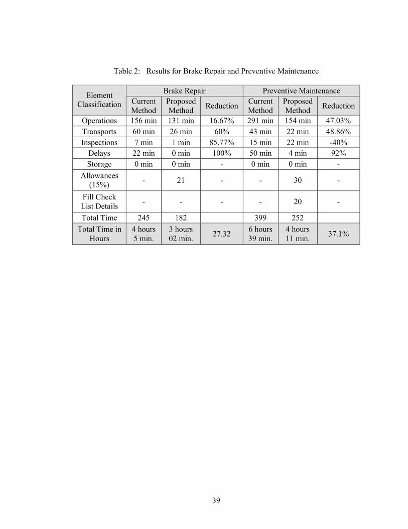
task in the specified time of the proposed standard (Centeno, 2002). Table 2 shows the
summary of results from the repair standard time developed for brakes (Centeno, 2002)
and PM jobs.
The time in the current method column reflects the time for one random
observation taken at a facility. The percentage reduction gives an estimate of the average
benefits from the standard developed. Most proposed standards take significant less time
than the current method observed. The average percentage of reduction is over 51%. As
seen in Table 2, all delays has been eliminated from the brakes job and reduced on 92%
of the cases for PM. There is however an increase in the time for inspections in PM.
This can be attributed to the fact that the technician working for that particular study may
be very experienced to handle the inspection sooner than the average or may have not
spent adequate time for the inspection.
39
Table 2: Results for Brake Repair and Preventive Maintenance
Brake Repair Preventive MaintenanceElement
Classification Current Method
Proposed Method
ReductionCurrent Method
Proposed Method
Reduction
Operations 156 min 131 min 16.67% 291 min 154 min 47.03%Transports 60 min 26 min 60% 43 min 22 min 48.86%Inspections 7 min 1 min 85.77% 15 min 22 min -40%
Delays 22 min 0 min 100% 50 min 4 min 92%Storage 0 min 0 min - 0 min 0 min -
Allowances (15%)
- 21 - - 30 -
Fill Check List Details
- - - - 20 -
Total Time 245 182 399 252
Total Time in Hours
4 hours 5 min.
3 hours 02 min.
27.326 hours 39 min.
4 hours 11 min.
37.1%

40
CHAPTER 5
DEMAND FORECASTING MODEL DEVELOPMENT
Transit facilities usually plan maintenance routines based on mileage or time
intervals depending on the process to be performed. Bus service manuals serve as guides
for the transit facilities to determine maintenance intervals and forecast inspection
requirements. The mileage interval recommended by the manufacturers assumes normal
driving and fair environmental conditions. However, the frequency to perform jobs may
vary according to the experience and judgment of the manager.
Major repairs can also be planned in advance by taking the manufacturer
recommendations as well as the maintenance historical information. For instance, air
conditioning (A/C) service is checked every time a PM is performed, but a deep
maintenance is recommended to take place every year before the summer season,
regardless of the mileage. Nevertheless, historical information shows that due to the
inefficient methods to plan and predict repairs there is a high incidence of road calls
(RC). For example, a high number of RCs on A/C jobs is typically seen during summer
season.
RCs are defined as the occurrences of an incident while the bus is providing
service. Accidents or break downs are examples for RCs. These types of calls are
41
difficult to predict and when they occur, the maintenance facility must be prepared to
take action immediately, and in an effective manner.
The objective of developing an effective forecasting approach is to accurately
represent the most probable occurrences of regular and unexpected repairs and to give
managers scenarios of possible incidences for opportune reactions. The forecasting
model presented does not specify which particular bus will fail but predicts occurrences
of breakdowns and anticipate fleet maintenance using historical information.
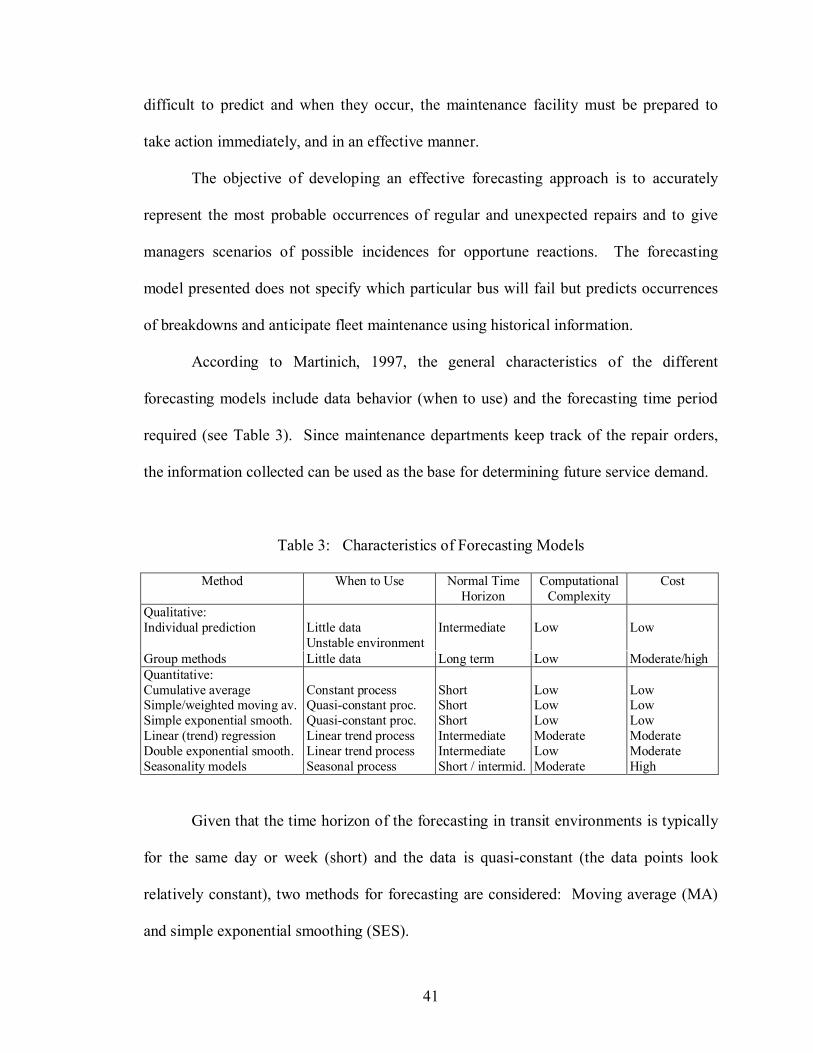
According to Martinich, 1997, the general characteristics of the different
forecasting models include data behavior (when to use) and the forecasting time period
required (see Table 3). Since maintenance departments keep track of the repair orders,
the information collected can be used as the base for determining future service demand.
Table 3: Characteristics of Forecasting Models
Method When to Use Normal Time Horizon
Computational Complexity
Cost
Qualitative:Individual prediction Little data
Unstable environmentIntermediate Low Low
Group methods Little data Long term Low Moderate/highQuantitative:Cumulative averageSimple/weighted moving av.Simple exponential smooth.Linear (trend) regressionDouble exponential smooth.Seasonality models
Constant processQuasi-constant proc.Quasi-constant proc.Linear trend processLinear trend processSeasonal process
ShortShortShortIntermediateIntermediateShort / intermid.
LowLowLowModerateLowModerate
LowLowLowModerateModerateHigh
Given that the time horizon of the forecasting in transit environments is typically
for the same day or week (short) and the data is quasi-constant (the data points look
relatively constant), two methods for forecasting are considered: Moving average (MA)
and simple exponential smoothing (SES).
42
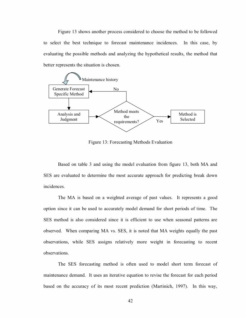
Figure 13 shows another process considered to choose the method to be followed
to select the best technique to forecast maintenance incidences. In this case, by
evaluating the possible methods and analyzing the hypothetical results, the method that
better represents the situation is chosen.
Figure 13: Forecasting Methods Evaluation
Based on table 3 and using the model evaluation from figure 13, both MA and
SES are evaluated to determine the most accurate approach for predicting break down
incidences.
The MA is based on a weighted average of past values. It represents a good
option since it can be used to accurately model demand for short periods of time. The
SES method is also considered since it is efficient to use when seasonal patterns are
observed. When comparing MA vs. SES, it is noted that MA weights equally the past
observations, while SES assigns relatively more weight in forecasting to recent
observations.
The SES forecasting method is often used to model short term forecast of
maintenance demand. It uses an iterative equation to revise the forecast for each period
based on the accuracy of its most recent prediction (Martinich, 1997). In this way,
Generate ForecastSpecific Method
Analysis andJudgment
Method meets the
requirements?
Method is Selected
No
Yes
Maintenance history

43
maintenance supervisors can forecast for the immediate future repair demand to
accurately estimate the scheduling needs ahead of time. This approach allows the
maintenance department to optimize the allocation of technicians for the jobs based on
their skills.
The following is the SES model formula:
Fd+1 = Fd + α (yd – Fd)
Fd+1 represents the forecasted number of maintenance jobs
Fd represents the number of maintenance jobs predicted for the day d
α is the smoothing constant
yd is the actual number of jobs performed and used as a data point.
The values of α can vary from 0 to 1 depending upon the rate of reaction required
for the maintenance department. A higher rate of reaction is represented by a value of α
close to 1. The α value is used to smooth out the inaccuracy, so that the maintenance
demand anticipations do not overreact when unexpected changes occur.
The MA approach represents the average of the N most recent data points (failure
incidences). The smaller value given to N represents a more responsive demand forecast.
The following is the MA formula:
Fd = (yd-n + yd-n+1 + … + yd- 1) / N
Fd represents the number of maintenance jobs predicted for the day d
N is the number of periods averaged
yd is the actual number of jobs performed and it used as a data point.

44
Table 4 shows the comparison of methods MA (N=2) and SES (α = 0.9) for a two
years demand of brakes system incidences. It also shows the accuracy of the methods by
computing the mean square error (MSE).
Table 4: Forecasting Methods Applied to RCs of Brakes Repair System
Brakes System Forecast
Month Years 02-04 Years 04-05 SES(α=0.9) MA(2 month)October 5 17 5November 5 19 5December 7 5 5 5January 10 7 6February 8 10 9March 3 9 9April 15 4 6May 8 14 9June 11 9 12July 7 11 10August 4 8 9September 6 5 6October 12 6 5November 6 12 9December 9 7 9January 6 9 8February 5 7 8March 14 6 6April 7 14 10May 6 8 11June 10 7 7July 10 10 8August 6 10 10September 14 7 8
Mean Square Error 21.958 18.545Standard deviation 2.771 1.918
Variance 7.679 3.680Average 8.125 8.182
Figure 14 shows both methods compared with the original data. As it is shown
SES model presents a similar path to the demand points; however, MA presents closer

45
demand points with respect to the actual demand. The method that reports less variance
is the MA.
Road Calls vs Forecasting Models
02
468
10
121416
1820
Octobe
r
November
Decem
ber
Janu
ary
Februa
ry
Marc
hApril
May
June Ju
ly
August
Septe
mber
October
November
Decem
ber
Janu
ary
Februa
ry
Marc
hApril
May
June Ju
ly
August
Septem
ber
Months
# of
Roa
d ca
lls
Years 02-04 Years 04-05 Simple E. Smoot. Moving Ave.
Figure 14: Actual Data vs. MA and SES for Brakes
RCs incidences due to brakes failure do not have consistency in terms of
seasonality; therefore, the MA method presents an advantage over the SES due to the
lower MSE. However, there are RCs incidences related to seasonal reasons which is the
case for A/C failures. This particular system presents peaks of repair demand during the
summer months. After applying the same analysis to the A/C demand, the two
forecasting methods reported 91.2 MSE and 98 MSE for SES and MA respectively.
However, the variance is very close showing 11.775 and 11.663 for SES and MA. Figure
15 shows the trend of demand for A/C failures from 2002 to 2004, as well as the two
forecasting models applied. The bars represent the actual demand and the two lines
represent the forecasting models.

46
Road Calls vs Forecasting Models
0
5
10
15
20
25
30
35
40
45
50
Octobe
r
Novem
ber
Decem
ber
Janu
ary
Febru
ary
Mar
chApr
ilM
ayJu
ne July
Augus
t
Septe
mbe
r
Octobe
r
Novem
ber
Decem
ber
Janu
ary
Febru
ary
Mar
chApr
ilM
ayJu
ne July
Augus
t
Septe
mbe
r
Months
# of
Roa
d ca
lls
Years 02-04 Years 04-05 Simple E. Smoot. Moving Ave.
Figure 15: RCs vs. Forecasting Models for A/C System
Peaks of demand make that the high variation between close data points be
smoothed resulting on giving the SES model as the most accurate estimator. However,
the MA also presents close estimations that can be valid to model future A/C failure
incidences. Due to the closest MSE and variances presented by the two methods, it is
necessary to analyze with detail the best method to be applied. A test of hypothesis for
the ratio of the two population variances is the used to evaluate the most accurate method.
The hypothesis testing is based on the F distribution presented as follow
(Mendenhall, Sincich, 1995). The null hypothesis H0 states that S1 (SES) and S2 (moving
average) corresponding to the brakes system demand forecast are equal. The alternative
hypothesis states that S1 > S2 and therefore S2 (moving average) is the most accurate method.
H0: S1 = S2 Null hypothesis
Where: S1 and S2 are the population variance for methods one and two
N1, N2 are the sample sizes for methods one and two

47
α is the level of confidence of T
Fo is the test statistic
The alternative hypothesis and the criteria for acceptance and rejection are:
Ha = S1 > S2 Reject if Fo > Fα
Degrees of freedom = 23 and 21 for populations N1 and N2
Level of confidence α = 0.05 06.205.0 F
Table 5: Test of Hypothesis for the Variances of MA and SES
Simple E. Smoothing Moving AverageMean 8.125 8.181818182Variance 7.679347826 3.67965368Observations 24 22Df 23 21F 2.086975703P(F<=f) one-tail 0.047439005F Critical one-tail 2.063280363
The results shown in table 5 demonstrate that Fo value equal to 2.087 exceeds the
tabulated value F0.05 (2.06). Moreover, the p value calculated (0.04) is less than the
maximum tolerated value that was stated for the test (0.05). As a result the null
hypothesis should be rejected. However, there is not enough evidence to state that the
MA method is more accurate than the SES method. To determine which method is more
effective or if the two models have the same effectiveness, a test of the difference
between the two population means is conducted.
μ1 and μ2 represent the mean of the SES and MA forecast respectively.
H0 : μ1 = μ2
Ha: μ1 > μ2

48
The t distribution based on n-1 degrees of freedom is based on a sample of 22
months. The null hypothesis will be rejected if t > t0.05 (1.721)
Table 6: t-Test: Paired Two Sample for Means (A/C Jobs)
SES MAMean 18.13636 17.68182Variance 151.5519 136.0368Observations 22 22t Stat 0.515319P(T<=t) one-tail 0.305856t Critical one-tail 1.720743
Since the value of the t statistic 0.515319 does not exceed the critical value t0.05
1.721, there is evidence at α = 0.05 to show that the null hypothesis cannot be rejected.
This conclusion can be also stated after analyzing the p-value of the test that shows a
greater value 0.305856 than the α =0.05 level selected. As a result, it can be stated that
the SES and MA forecasting methods are equal and therefore either of them can be used
to predict repair jobs at transit facilities.
After evaluating the two methods with SES (α=0.9) and MA (2 month average), it
is important to assess the optimal factor of smoothing in any of the methods to be
applied. In this case a comparison between MA (4 months average) and MA (2 months
average) is performed using a t-test on the difference between the two population means
for RCs in A/C system.
μ1 and μ2 represent the mean of the MA(2 month average) and MA(4 month average)
forecasts respectively.
The null hypothesis states that μ1 = μ2
The alternative hypothesis states that μ1 < μ2

49
The t distribution based on n-1 degrees of freedom is based on a sample of 20
months. The null hypothesis will be rejected if t < -t0.05,19 (1.729)
Table 7: t-Test: Paired Two Sample for Means (MA)
2 month ave. 4month ave.Mean 18 18.6Variance 107.0526316 138.4631579Observations 20 20Pearson Correlation 0.867184562Hypothesized Mean Difference 0df 19t Stat -0.45777595P(T<=t) one-tail 0.326152644t Critical one-tail 1.729132792
The value of the t statistic -0.4577 is not less than the negative value of t0.05,19
1.729, there is evidence at the 0.05 level of significance to show that the null hypothesis
cannot be rejected and the moving average forecasting methods with 2 and 4 months
average are equals for the type of demand studied. However, since the MSE1 (98) <
MSE2 (183.85), the method that applies 2 months of average is recommended.
5.1 Forecasting Model Applied to Failure Incidences
Data from the historical record of incidences is used to model the future possible
occurrences with MA (two months) method. The selected forecasting model is applied to
real data that comes from the historical information of failure incidences at a transit
facility. Table 8 presents a monthly forecasting model for engine failures on a period of
one year.

50
Table 8: Possible Monthly Outcomes of Engine Repairs for Year 2005
RCs - Engine System ForecastMonths Year 02-04 Year 04-05 MA (2-month)
October 23 21November 8 22December 18 15 16January 14 13February 15 16March 19 15April 18 17May 20 19June 19 19July 19 20August 12 19September 16 16October 17 14November 15 17December 13 16January 9 14February 26 11March 21 18April 15 24May 16 18June 7 16July 23 12August 19 15September 27 21
MSE 31.545S 2.211
After the data is analyzed, it can be noticed that for engine system, the months of
December reported 18, 13 and 15 cases for years 2002, 2003, and 2004 respectively and
the forecasted value was 16. If this method would have been used in December 2005, the
department could have reacted effectively to the demand. This is an interesting case for

51
this type of repairs since inventory related with engines is usually expensive and difficult
to maintain.
The data is then plotted to visualize the reaction of the estimated data to the actual
demand. Figure 16 presents the RCs for years 2002 to 2004 versus the forecasted
demand by using MA. The bars represent the past demand and the RCs for the months
10, 11, and 12 of 2004. The line shows the reaction to the demand using MA (2-months
averaged).
Road Calls Vrs Forecast with MA
0
5
10
15
20
25
30
Octobe
r
Novem
ber
Decem
ber
Janu
ary
Febru
ary
Mar
chApr
ilM
ayJu
ne July
Augus
t
Septe
mbe
r
Octobe
r
Novem
ber
Decem
ber
Janu
ary
Febru
ary
Mar
chApr
ilM
ayJu
ne July
Augus
t
Septe
mbe
r
Road Calls - Engine System Year 04-05 MA (2-month)
Figure 16: RCs (02-04) vs. Forecast with MA for Engine System
As it is shown in the graph, February 2003 presented an unusual peak of demand
that was not closely marked by the model. However, it can be also seen that there is a
rapid reaction to the demand presented for the majority of the year.
The forecasting developed would help managers to plan maintenance operations
on a monthly basis. In this way, the facility can have parts in inventory before a

52
breakdown occurs, thus buses will not stay idle for a long period of time. For example,
by knowing the typical occurrence of engine breakdowns, the facility could keep a
determine number of engines in stock or prepare providers on just in time delivery.
In the short time or daily basis, the modeling of repair occurrences could be useful
to plan shifts in terms of labor needs, shop capacity and bays allocation. Forecasting and
analyzing RCs is important for maintenance supervisors to get insights of how to improve
preventive maintenance jobs. By using the PM time standards model, more tasks could
be included in the process and some components could be replaced before they break and
damage other associated components. For example, including an exhaustive A/C
maintenance before summer time would reduce the high incidence of this type of
breakdowns.

53
CHAPTER 6
THE SCHEDULING MODEL
In this study a mathematical scheduling model that considers a finite number of
jobs, bays, and days is designed to allocate resources in transit maintenance facilities.
The model takes into consideration repair jobs demand forecasted, the repair time
standards and the technicians’ performance level. Two levels of scheduling are
suggested for the transit facilities: short time and long time horizon. In a short time
horizon, maintenance supervisors allocate resources for a single shift on a day. In a long
time horizon managers can use the scheduling to plan facility operations and make
decisions ahead of time for a month period or a quarter. The next section describes in
detail the model developed and its application for a short and long period of time.
6.1 Basic Model
The main objective of this scheduling model is to serve the maximum number of
vehicles that require any type of repair. This model allocates the most qualified
technicians (highest performance) to a required job. The performance level represents a
dependable input variable that comes as a result of the repair time standards. The model
also considers the repair time standards as a fundamental component when allocating
buses to bays during a working shift. The scheduling model is as follows:

54
MAX
b
i
t
k 11
Pik Xik (1)
Subject to:
b
i 1
Xik <= Dk k =1.. t (2)
t
i 1
STkXik <= Ti i = 1.. b (3)
Xik >= 0 and Integer (for all i and k) (4)
Where:
Xik =
Pik = performance level for technician i to do job k
STk = standard time for job k
Dk = total demand for job k during a shift
b= Total number of bays available in the facility
i = Bay index
t = Total number of jobs performed at the facility (PM, brakes, engine, RCs, etc.)
k = Job index
Ti = Total time available per bay (it is usually set to 480 minutes)
Equation (1) represents the scheduling objective which is to maximize the number
of jobs processed assigning the technicians with the highest performance level. Equation
(2) represents the first constraint which corresponds to the demand based on the
forecasting model or from the facility immediate needs. Constraint (3) accounts for the
total time on a shift. Constraint (4) is the nonnegative condition for variable X.
1, if the job k is assigned to bay i0, if the job k is not assigned to bay i

55
6.2 Extended Model
The following extended model includes factors such as shifts and time horizon.
The model is capable of scheduling different jobs for one-month period, considering
three shifts, eight hours a day, and a maximum of 10 bays. The following notation is
used:
b= Total number of bays available in the facility
i = Bay index
s= Total number of shifts
j = Shift index
t = Total number of jobs performed at the facility (PM, brakes, engine, RCs, etc.)
k = Job index
d= Total number of service days at the facility
l = Day index
we= Total number of weeks to be scheduled in the time horizon
m = Week index
Xijklm =
Pik = the performance level for technician i to a job k
STk = Standard time to perform a job “k”
wk = weight given to a job based on urgency of the repair completion (the higher
the need, the higher the weight). If there is no preference wk is equal to one.
Dk = Demand of job “k”
Ti = Total time available per bay (it is usually set to 480 minutes)
1, if the job is assigned to bay i, shift j, task k, day l, and week m0, if the job is not assigned in bay i, shift j, task k, day l, and week m

56
The formulation of the model is presented as follows:
MAX
we
m
d
l
t
k
s
j
b
i1 1 1 1 1
wk Pik Xijklm (5)
Subject to:
we
m
d
l
s
j
b
i1 1 1 1
Xijklm <= Dk k = 1..t (6)
t
k 1
STk Xijklm <= Ti j = 1..s l = 1..d
m = 1..w (7)
Xijklm >= 0 and Integer (8)
The objective function (5) maximizes the number of buses served daily. Pik
represents the factor that maximizes the equation since technicians with the major
performance level are assigned first before those who have low performance level.
Variable wk represents the weight given to a type of job that has priority on completion
over the others.
The constraints are represented by the repair and inspection jobs needed during
the time horizon should be accomplished in a daily basis. If the capacity is not enough to
cover a higher demand, the jobs must be scheduled for the following shift or day.
However, if the demand is low, the model still gives the maximum possible number of
jobs that can be performed in the bay thus managers can react rapidly to unexpected
repairs. This is reflected in constraint (6). Constraint (7) evaluates the total number of

57
jobs that can be allocated in each bay per shift depending upon the total hours worked per
shift, the model allocates as many jobs as possible by using the repair standard times.
Constraint (8) is nonnegative condition for variable X.
6.3 Heuristic Approach
The scheduling model takes advantage of the repair time standards to show the
possible combination of jobs that can be allocated in a single shift. Since it is assumed
that the transit facility has a shop for the repairs and a shop to perform the preventive
maintenance, it is recommended that a specific type of jobs be performed in every shift.
From the results of the repair time standards, up to two brake jobs can be now
served in one bay per shift. Moreover, one PM -12K job can be scheduled in bay per
shift. However, the remaining time after the PM is performed is recommended to be used
on process improvements or additional jobs.
For testing purposes, the time estimated for RC is set for 480 minutes since this
kind of job requires going through a process of diagnosis and then the repair is
performed. For the case of engine replacement, the time assigned is 480 minutes since
these jobs take approximately two days to be completed. The possible combinations of
service are found with a simple scheduling approach and put in the IMIS.
Computational complexities related with the high number of variables and the
optimal model requires the development of a heuristic approach. This section presents
the algorithm developed to solve the scheduling model. It is based on the selection of
jobs to be distributed as well as on the selection of bays available to allocate the buses.
The model flow and algorithm are presented as follows:

58
Initialize variables.Set b = 1…10; tb = 480; k = 1 = RCs, 2 = engine replacement, 3 = brakes; i = 1..10; pik denotes the performance level for technician i in job k; stk is the standard time for job k; dk is the demand for job k; and ti is the total time available in bay i.
If demand of job 3 is greater or equal than 16 and demand of job 1 is greater than1 then find the maximum performance level of technicians in job 1. If the time in bay where the technician is found is equal to the total bay time, then assign the job 1 to the bay and technician i. Subtract one job 1 from demand of job 1. If the time of bay i becomes zero then the bay is full and no more jobs can be assigned to it.
If demand of job 3 is greater or equal than 16 and demand of job 2 is greater than 1 then find the maximum performance level of technicians in job 2. If the time in bay where the technician is found is equal to the total bay time, then assign the job 2 to the bay and technician i. Subtract one job 2 from demand of job 2. If the time of bay i becomes zero then the bay is full and no more jobs can be assigned to it.
Start the cycle to assign brake jobs. Repeat it while there are still available baysor there is demand for job 3. Find the maximum performance level of technicians in job 3. Assign the job 3 to the bay and technician i. Subtract one job 2 from demand of job 2.Subtract the standard time for job 3 from the time available in bay i.If the number of job 3 assigned to bay i is equal to 2 or the demand of job 3 is 0, then no more jobs can be assigned to bay i.
Start the cycle to assign remaining jobs type 1 and 2.If demand of job 3 is equal to zero, and there is still demand for job 1, then find the maximum performance level of technicians in job 1.If the time in bay where the technician is found is equal to the total bay time, then assign the job 1 to the bay and technician i.Subtract one job 1 from demand of job 1.If the time of bay i becomes zero then the bay is full and no more jobs can be assigned to it.If demand of job 3 is equal to zero, and there is still demand for job 2, then find the maximum performance level of technicians in job 2.If the time in bay where the technician is found is equal to the total bay time, then assign the job 2 to the bay and technician i.Subtract one job 2 from demand of job 2.If the time of bay i becomes zero then the bay is full and no more jobs can be assigned to it.

59
6.4 Model Testing and Results
The model is tested using a scenario of scheduling for RCs, engine replacement,
and brakes. The standard time developed for brakes is 182 minutes, the engine
replacement time would be 480 minutes, and the stipulated time for RCs is 480 minutes.
Some other assumptions are necessary to test the model. For example: at least one
technician will correspond to a working bay and each of them will be assigned to the
same bay everyday. This assignment would facilitate the allocation of fixed working
places for technicians. The demand comes either from the forecasted data or from
demand received during the day.
The possible outputs can be applied to any required day or shift depending upon
the demand presented. The capacity of the shop is set for ten bays within a shift of 8
hours. The heuristic approach assigns at least one RC and one engine job if the brakes
demand exceeds 16 jobs. In this way, at least 8 bays are assigned to brakes and one bay
for a RC and one for an engine replacement. This assignment facilitates the allocation of
higher number of minor repairs to prevent major breakdowns.
The algorithm was coded in Matlab version 7.0 (See Appendix 1). The outputs
for a shift with the simulation of different demands are shown below.
General data Input:
Total time per shift = 480 minutes Standard time for brakes = 182 minutes Time for engine replacement= 480 minutes Time for RCs jobs = 480 minutes Number of bays = 10 Number of technicians = 10 Performance level = classification according to the technicians’ actual
performance. It is shown in table 6 and the number of significance is: 0.9: below the standard (actual performance <= 94%)

60
1.0: on the standard (95% <= actual performance <= 104%) 1.1: above the standard (actual performance >= 105%)
Table 9: Performance Rating for Technician i on Job k
Job 1 2 3 4 5 6 7 8 9 10RC 0.9 1.1 1.0 1.0 0.9 1.1 0.9 1.0 0.9 1.0ENG 1.0 1.1 0.9 1.1 1.0 0.9 1.0 1.1 1.0 0.9BRK 1.1 0.9 1.0 0.9 1.1 1.0 1.1 0.9 1.1 1.1
The scenarios of demand and distribution are shown in the following tables. They
reflect a distribution of jobs based on giving priority to the most frequent jobs and to
those with the lowest standard time. However, if the demand of jobs with the lowest
standard time exceeds the capacity, at least one less frequent job and with highest
standard time will be allocated if demand exists. For example, if the demand of brakes
jobs exceeds 16, this means that the shift resources would be covered only with brakes
jobs. However, if there is at least one job required for engine or RCs, the system will
assign the technicians with the highest performance level on RC and engine to each bus
and bay. After that assignment is done, the brakes repairs are allocated in the remaining
bays. Scenario 1 of assignment presented in table 10 shows the distribution resulted for a
demand of 4 RC, 2 engine replacement and 10 brakes.
Table 10: Outcomes of the Objective Function for Scenario 1
Number of jobs allocated per bay
Jobs 1 2 3 4 5 6 7 8 9 10
RC 0 1 1 0 0 1 0 0 0 0
ENG 0 0 0 1 0 0 0 1 0 0
BRK 2 0 0 0 2 0 2 0 2 2
Similarly the outcomes for constraint 6 (demand) are presented as follow:

61
Road calls demand and assigning X1 = 3 <= D1 = 4
Engine demand and assigning X2 = 2 <= D2 = 2
Brakes demand and assigning X3 = 10 <= D3 = 10
The outcomes for constraint 7 (time per shift) are shown in table 11.
Table 11: Outcomes for Constraint 7 – Scenario 1
Utilization time per bay (minutes)Jobs 1 2 3 4 5 6 7 8 9 10RC 451 480 455ENG 455 455BRK 342 348 348 348 348
Scenario 2 shows the distribution that will satisfy a demand that exceeds the 16
brakes and assign first one engine and one RC and then the maximum number of brakes
that could be allocated. This scenario responds to a demand of 4 RC, 5 engine
replacement and 17 brakes. The outcomes of the objective function are presented in table
12 as follows:
Table 12: Outcomes of the Objective Function for Scenario 2
Number of jobs allocated per bay
System 1 2 3 4 5 6 7 8 9 10
RC 0 1 0 0 0 0 0 0 0 0
ENG 0 0 0 1 0 0 0 0 0 0
BRK 2 0 2 0 2 2 2 2 2 2
The outcomes for constraint 6 (demand) are presented as follow:
Road calls demand and assigning X1 = 1 <= D1 = 4

62
Engine demand and assigning X2 = 1 <= D2 = 5
Brakes demand and assigning X3 = 16 <= D3 = 17
The technician’s performance level is not only the factor that permits the
maximization of the number of jobs to be performed but also improves productivity in
terms of completion time. The outcomes for constraint 7 (time per shift) are shown in
table 13 and demonstrate how the assignment of technicians with the highest performance
level enhances the time available in the bay to improve the processes or have the bay
clear to unexpected needs.
Table 13: Outcomes for Constraint 7 – Scenario 2
Utilization time per baySystems 1 2 3 4 5 6 7 8 9 10RC 455ENG 455BRK 348 364 348 364 348 384 348 348
The third scenario represents the case when the demand exceeds the capacity of a
shift. For this case 30 brakes repairs, 20 engines and 20 road calls need to be scheduled.
Given that brake repair takes much less time than engines or road calls, the maximum
number of brakes should be scheduled but without disregarding the other type of jobs.
For that reason, brakes are assigned to 16 bays (2 jobs to 8 bays) and to the other two
bays one engine and one road calls jobs are assigned. ) The unsatisfied demand would be
scheduled similarly in the following day by using the same distribution of jobs. Table 14
presents the allocation of jobs for every shift.

63
Table 14: Outcomes of the Objective Function for Scenario 3
Number of jobs allocated per bay
System 1 2 3 4 5 6 7 8 9 10
RC 0 1 0 0 0 0 0 0 0 0
ENG 0 0 0 1 0 0 0 0 0 0
BRK 2 0 2 0 2 2 2 2 2 2
The outcomes for constraint 6 (demand) in scenario 3 are presented as follow:
Road calls demand and assigning X1 = 1 <= D1 = 20
Engine demand and assigning X2 = 1 <= D2 = 20
Brakes demand and assigning X3 = 16 <= D3 = 30
The outcomes for constraint 7 (time per shift) are shown in table 15.
Table 15: Outcomes for Constraint 7 – Scenario 3
Utilization time per baySystems 1 2 3 4 5 6 7 8 9 10RC 455ENG 455BRK 348 364 348 364 348 384 348 348
Scenario 2 and 3 presented a similar distribution due to the existence of engine
and RC demand and brakes repair requirement greater than the number of bays. Scenario
4 presents no brakes demand and a high requirement of engine and RC jobs. In this case
the jobs are distributed on a 50%-50% basis. The demand for this scenario is 30 jobs for
engine and RC respectively.

64
Table 16: Outcomes of the Objective Function for Scenario 4
Number of jobs allocated per bay
System 1 2 3 4 5 6 7 8 9 10
RC 0 1 1 0 0 1 1 0 0 1
ENG 1 0 0 1 1 0 0 1 1 0
BRK 0 0 0 0 0 0 0 0 0 0
The outcomes for constraint 6 (demand) in scenario 3 are presented as follow:
Road calls demand and assigning X1 = 5 <= D1 = 30
Engine demand and assigning X2 = 5 <= D2 = 30
Brakes demand and assigning X3 = 0 <= D3 = 0
The outcomes for constraint 7 (time per shift) are shown in table 17.
Table 17: Outcomes for Constraint 7 – Scenario 4
Utilization time per baySystems 1 2 3 4 5 6 7 8 9 10RC 455 480 455 509 480ENG 480 455 480 455 480BRK
The system provides options of bus allocation that can be used to plan
maintenance schedules in a daily basis. The database is configured with the scenarios
generated that will assist supervisors in the decision making process.

65
6.5 Productivity Measurement
The scheduling performance is measured based on the productivity improvement
of the maintenance facility. The quantity of jobs that can be allocated with the integrated
scheduling model are compared and tested against the current method to demonstrate
improvement in utilization and productivity, and effectiveness when assigning
technicians according to their performance level to the required tasks.
The current method of scheduling is based on the average completion time
calculated in the repair time standards study. This time is rounded to 240 minutes and
although it seems like two jobs can be allocated, only one job is actually assigned per
shift due to the lack of consistency in completion time. Some technicians may take less
than the 240 minutes and some may take much more time to complete the job. On the
other hand, the time standard developed suggests 182 minutes per job, enough time to
complete two jobs per bay. Table 18 shows the comparison of the percentage of
utilization per bay when allocating brake jobs. The productivity improvement is noticed
when the demand of jobs exceeds the capacity of the facility.
Figure 17 shows the productivity improvement from a random distribution of
brake jobs to be scheduled shown in table 18. This figure shows the difference between
the number of jobs that can be accomplished by following the current method (with only
one job assigned per bay), versus the new method that permits the allocation of two brake
jobs per bay. Moreover, the assigning of two jobs still presents some time remaining that
could be used either to allocate a job with small completion time or to improve the
current repair process.

66
Table 18: Percentage of Utilization per Bay – Current Scheduling
Demand of buses per day
Current number of jobs scheduled
Maximum possible jobs with new model
# of jobs Productivity
# of jobs
Productivity PL 90
Productivity PL 100
Productivity PL110
15 10 38% 15 53% 57% 60%20 10 38% 20 71% 76% 80%8 8 30% 8 29% 30% 32%5 5 19% 5 18% 19% 20%
18 10 38% 18 64% 68% 72%22 10 38% 20 71% 76% 80%17 10 38% 17 61% 64% 68%30 10 38% 20 71% 76% 80%25 10 38% 20 71% 76% 80%2 2 8% 2 7% 8% 8%
10 10 38% 10 36% 38% 40%7 7 27% 7 25% 27% 28%
16 10 38% 16 57% 61% 64%28 10 38% 20 71% 76% 80%24 10 38% 20 71% 76% 80%
Media 8.8 33% 14.53 52% 55% 58%
Brakes Jobs Productivity Improvement
0%10%20%30%40%50%60%70%80%90%
15 20 8 5 18 22 17 30 25 2 10 7 16 28 24
# of Jobs
Productivity Productivity PL 100Productivity PL110 Productivity PL 90
Figure 17: Productivity Improvement – Brake Jobs

67
CHAPTER 7
THE INTEGRATED MAINTENANCE INFORMATION SYSTEM
In this chapter, the database development is presented and the models are applied
to a typical transit maintenance facility. The current situation related to repair time
standards, forecasting, and scheduling is discussed and then compared with the proposed
model.
7.1 Database Specifications
The database development was performed in parallel to the systems/models
development. The IMIS gathers the information from the models developed, and serves
as for a planning tool. It is designed and run in Microsoft Access® for the benefit of the
final users since it is a software easily available commercially. The database designed for
the repair time standards research is the base for the development of the IMIS.
The database has the information stored in tables represented by “employee”,
“vehicle”, “system”, “shift”, “daily schedule”, “work order”, among others. For each
table there are a number of entities that gives characteristics to the type of information
stored. Each entity has a name, data type and description. Figure 18 shows the table
“employee” with its entities represented by fields, type and description.

68
Figure 18: Table Employee – Fields, Data Types and Description
A relational database facilitates the interaction between any two tables.
Establishing connection among tables eliminates data redundancy and ensures confidence
when accessing data. The relationships can be classified into one-to-one, one-to-many,
many-to-many, or no relation depending upon the type of data shared by the tables and
the characteristics of the fields shared.
Figure 19 shows the architecture of the table relationship of the IMIS. As it is
seen in the figure, most of the tables have correlative relation with the employee table.
Tables that are linked to work orders have a relation with employee automatically.

69
Figure 19: Table-Relationship Diagram
7.1.1 Database tables: In this section the most relevant tables are discussed. This
includes information regarding employee, vehicle, system, process, daily schedule and
work order. All the information entered into the system through a form is stored in the
corresponding tables as it is shown in figure 20.
Figure 20: Information Stored in Table “Employee”

70
Other relevant tables in which data are manipulated include: vehicle, system,
daily schedule, and work order. Table 19 shows the fields and content of table system.
This table is important for the IMIS because it contains the standard time for each job.
The standard time for brake repairs and PM (12K) where developed following the
methodology presented in chapter 4.
Table 19: Table System
systemcode systemname stdtimemin stdtimehours
Brake Brake 182 3 Hours 2 Min
PM (12k) PM 251 4 Hours 11 Min
Table 20 corresponds to the data that identify the vehicles. This information
pertains to the buses observed during repair time standards study.
Table 20: Table Vehicle
busid make model length fueltype startMiles details
2001 Flexible 3454 40 Foot Diesel 0
2002 Flexible C1221 1994 40 Foot LPG 0
2003 Flexible 3454 40 Foot Diesel 0
9603 Gillig Phantom 40 Foot Diesel 0
9604 Gillig Phantom 40 Foot Diesel 0
9605 Gillig Phantom 40 Foot Diesel 0
9701 Gillig Phantom 40 Foot Diesel 0
9702 Gillig Phantom 40 Foot Diesel 0
9703 Gillig Phantom 40 Foot Diesel 0
9801 Gillig XT 1400 MAY 2000 40 Foot Diesel 0
Table 21 shows the daily schedule table and how the system stores information
about the current or forecasted demand as well as the shift and the person who developed
the scheduling.

71
Table 21: Table Daily Schedule
sche
dule
id
sche
dule
date
sche
dule
shif
t
sche
dule
dem
and
nam
e
brkd
em
engi
dem
rcal
ldem
brkd
em2
brkd
em1
engi
dem
2
engi
dem
1
Rca
llde
m2
Rca
llde
m1
14 3/3/2005 Morning 10 Gilbert Seward 5 2 315 3/3/2005 Night 17 Gilbert Seward 13 2 216 3/10/2005 Afternoon 46 Adam Sandler 10 32 4 10 10 55 10 3 4
17 3/10/2005 Afternoon 7 Charles Wolf 2 2 3 3 2 1 2 2 4
As it is seen in the table, jobs with schedule id 14 and 15 (shown in column 1)
represent an input of current demand. In other words, no previous demand was entered
therefore the demand is not forecasted. On the other hand, jobs with schedule id 16 and
17 (shown in column 1) have a total demand (see brkdem, engidem, and rcalldem fields
shown in columns 6, 7, and 8) forecasted by using previous data.
7.1.2 Database input forms: The interface system-user is one of the most important
components in a computerized system. Users should be able to enter the information in a
straightforward way. In this section, three of the most relevant forms in which the
information is managed are discussed, the “employee data input” form, the “daily
schedule” form, and the “work order” form.
The “employee data” form is used to input basic data into the system. It requires
basic information of the vehicle, system, and process. Figure 21 presents an example of
the interface of the IMIS.

72
Figure 21: Employee Data Form
Planning the scheduling is one of the most important applications of the IMIS.
The form “daily schedule” is intended to facilitate this process to the supervisors. This
form gives the users the option of entering current data or forecasting possible situations.
Users also are required to input the name of the person who prepares the schedule as well
as the shift for which the schedule is done. Figure 22 shows the screen for scheduling
input.
Figure 22: Daily Scheduling Form
The form “work order” is the interface to input information regarding jobs done.
Technicians or supervisors are required to input the starting and ending time for the job to

73
calculate the technician’s performance level and also to records the maintenance history.
Figure 23 shows the screen for work order input.
Figure 23: Work Order Form
7.2 Application
The example discussed represents a public transit organization that serves a
middle type of city and population in the state of Florida. This includes an average
population of 3,000,000 in the area and approximately 20% of this population is served
by the public transit service. The company operates with 200 diesel buses and
approximately another 120 vehicles that connect services with the buses.
Historical data regarding maintenance tasks incidence is analyzed to forecast a
feasible path of jobs demand. This is mostly applied to those jobs that are very difficult
to forecast due to the uncertain demand, e.g., RCs. Jobs such as PM, engine and
transmission repairs are basically scheduled based on mileage intervals, therefore are less
difficult to predict. To forecast demand of maintenance jobs is the main goal for
designing the scheduling model, considering availability of bays, technician’s skills and
the deadline for the repairs.
Most transit facilities have fixed routes and their vehicles operate on
predetermined timetables. This facilitates the forecasting of certain repair jobs and bus

74
maintenance. This research shows a scheduling model that combines PM and brake time
standards with forecasting information to allocate buses for repair in an eight-hour shift.
By integrating the scheduling model with time standardization, transit maintenance shops
can optimize resource utilization and improve the response capacity to unexpected
breakdowns.
The transit facility studied does not use time standards to schedule resources;
therefore, it is capable of allocating only one job per bay per shift no matter what the total
time of the job is. If the technician is not able to finish the job during the shift he has the
option of parking the bus aside to leave the bay empty for the next shift or he has the
option of transferring the work order to the technician of the following shift.
Our study shows that based on the repair time standards for brake jobs, up to two
brake jobs could be allocated to a bay and technician in a single shift. Also, one PM
(12K) can be allocated in a bay and the remaining time can be used to improve
maintenance processes or to allocate a shorter PM depending upon the service needs.
Road calls and engine replacement standards are under development, but 480 minutes
have been assumed and inputted into the database.
The modeling of forecasted demand is evaluated in Chapter 5 with data for a
month period. This information can be also used by supervisors to estimate the demand
for subsequent shifts.
The scheduling model is used as a tool to find the possible combinations of jobs
to be allocated per shift. All the scenarios that resulted from the combination of PM jobs,
RC, engine replacement, and brake repairs are included in the database.

75
The Integrated Maintenance Information System assists maintenance supervisors
when evaluating workforce productivity and identifying needs of training. Therefore,
some of the most important reports generated by the database are related to the
performance level rate. With these reports, users can opt to obtain information as a list or
as a graph. Figure 24 shows the graphical format report for a combined performance
level of brake repairs and PM jobs. It shows the performance level grouped in three
categories, below standard, standard, and above standard. The performance level report
gives the managers a general idea of how the technicians are performing in comparison to
the standards. The system also gives a listed report that specifies the actual performance
per job and technician which is summarized in the graphical report. The performance
level generated from the time standards is used to generate a report with the list of the
technicians with their respective performance level in every shift.
0
1
2
3
4
5
6
7
8
# of
Job
s
90 100 110
Performance Level
Combined Performance Level Report
Brakes
PM
Figure 24: Graphical Report for Performance Level (Brake and PM Jobs)

76
The possible combinations of job allocation is also included in the database to
facilitate the decision making process for supervisors at every shift. Figure 25 shows a
partial list of job combinations that are included in the system. The scenario is based on
the distribution of brake jobs, road calls, and engine replacement. These combinations
distributed by technician’s performance level were discussed in detail in Chapter 6.
Figure 25: Scenarios of Scheduling Based on Standard Times
With the system supervisors will be able to input information regarding jobs
demand. Reports that show the possible distribution of jobs and the list of technicians
available for the shift with their respective performance level are then generated. Figure
26 shows the system interface used by supervisors to input the demand per shift. A list of

77
technicians available for the shift and their respective skills type can be printed for
records.
Figure 26: Database Input Form – Daily Scheduling
The list of technicians available for a normal shift scheduling is shown in figure
27.
Figure 27: List of Technicians Available for a Morning Shift Scheduling

78
CHAPTER 8
CONCLUSIONS AND FUTURE RESEARCH
8.1 Conclusions
In this study a scheduling model that combines repair time standards with
forecasting methods has been developed. The contribution of this study is the
combination of approaches that gives managerial applicability to the administration of
transit maintenance departments. Better planning of repairs will result in cost savings,
timely maintenance and reduction of road calls which translates into better and more cost
effective transit service.
The model is useful to facilitate the process of resource planning on a monthly
basis and the resource allocation on a daily basis. It assumes that the facility has different
shops to perform repairs and PMs; each shop would have at least 10 bays and at least the
same number of technicians to work in every shift.
The repair time standards developed are the result of a methodological study
performed at three transit facilities and shows the process and time standardization for
brakes and PMs. The forecasting model uses the moving average mathematical approach
assigning a higher importance to the last two maintenance period demands for each
system. The scheduling is formulated as a mathematical method and it can be applied to
any maintenance system.

79
The results from the repair time standardization, as shown in section 4.1, reveal a
significant reduction for the required time for complete brake repairs and PMs. Both
systems present modular approaches that in practice represent a 27.20% and a 37.14%
time reduction, respectively. The time for the first system is decreased by 67 minutes and
for the second system is decreased by 148 minutes.
The forecasting method uses the maintenance historical data to model estimations
of demand. Road calls are modeled and possible occurrences for the next two years are
predicted. This information is useful to the managers as they can use it to schedule
preventive maintenance before the breakdowns occur. The model has been tested and
validated statistically.
The scheduling model is also capable of assigning the jobs to the most qualified
technicians. It has been demonstrated that productivity can increase from 33% to 58% on
average when technicians are assigned to perform brake jobs in a single shift. Moreover,
when the jobs are assigned to the technicians with the highest performance level,
additional time is gained to improve the maintenance processes.
The integrated maintenance information system is a user friendly application
developed to assist maintenance managers and supervisors in the planning process of
resource allocation. It presents various forms which are used to input or modify
information regarding employees, fleet, daily scheduling or work orders. A series of
relevant and useful reports have been designed and proven to be useful to managers.
These reports are easy to read and are designed to fulfill the maintenance users’ needs.

80
8.2 Future Research
Ongoing extensions of the current research toward the optimization of operations
in maintenance departments of transit companies include:
The standardization of all systems repaired in the facilities and for new fleet
technologies. Accurate standards represent an important issue to improve
maintenance processes. Furthermore, incorporating time standards of other repair
jobs will enrich the scheduling model.
The scheduling developed assumes that when a job is assigned to a bay, needed parts
for the repair are always available in the warehouse. Inventory policy for spare parts
is a constraint that can be added to the scheduling model to administrate the allocation
of resources. Engines and transmissions are examples of very expensive parts that
companies prefer to order when needed rather than having them in inventory. The
availability of parts can limit the effectiveness of the scheduling model.
A study to evaluate if the technicians should be scheduled based on the types of jobs
required is recommended. That is, after developing the repair time standards for all
the systems it might be better to do only brake jobs during a given shift. If that is the
case, only the technicians that have high performance level on that skill should called
in to work. This consideration could enhance the optimization of the resources.
Improvements on the IMIS are encouraged to make the system more complete and
manageable for users. The system could be moved to a version that allows easy
migration of data to common information systems used by the transit organizations.

81
REFERENCES
Boldt, R., 2000. TCRP Synthesis of Transit Practice 35: Information Technology Update for Transit. Transportation Research Board, National Research Council, Washington D.C.
Centeno, G., 2002. Repair Time Standards for Transit Vehicles-Final Report, Project BC137-RPW032, Florida Department of Transportation, Tallahassee.
Centeno, G., Chaudhary, R., Lopez, P., 2005. A Systematic Approach for Developing Standard Times for Repair Activities in Transit Vehicles. Paper in presssubmitted to Transportation Research Board, National Research Council, TRB annual conference. Washington D.C. 2005.
Etschmaier, M.M, 1985. Transit Bus Maintenance Management in the United States. Transportation Research Part A, 19, 1-14.
Etschmaier M.M., Anagnostopoulos, G., 1984. Systems Approach to Transit Bus Maintenance. Transportation Research Record, Transportation Research Board, National Research Council, Washington D.C.
Federal Transit Administration. 2001. Development of a Model Transit Bus Safety program. http://transit-safety.volpe.dot.gov/safety/bustasks/task3/pdf/task3.pdf.
Florida Department of Transportation. Transit 2020 Plan: A Strategic Plan for Public Transportation. http://www.dot.state.fl.us/transit/Pages/transit2020plan.htm.
Guenthner, R.P., Sinha, K.C., 1983. Maintenance, Schedule Reliability and Transit System Performance. Transportation Research Part A.
Haghani, A., Shafahi, Y, 2001. Bus Maintenance Systems and Maintenance Scheduling: Model Formulations and Solutions. Transportation Research Part A, 36, 453-482.
Hall, R.W, 2000. Scheduling Transit Railcar Maintenance and Facility Design, Transportation Research Part A, 34, 67-84.
Hillsborough Area Regional Transit Authority (HARTLINE). http://www.hartline.org/.

82
Hillsborough County Metropolitan Planning Organization (MPO). 2025 Long Range Transportation Plan. Adopted November 13, 2001; amended April 15, 2003 http://www.hillsboroughmpo.org/about/index.htm.
Inaba, K, 1984. Allocation of Time for Transit Bus Maintenance Functions. Transportation Research Record, Transportation Research Board, National Research Council, Washington D.C.
Krajewski, L., Ritzman, L., 1990. Operations Management: Strategy and Analisis. Addison-Wesley Publishing Company, Inc. Westerville, Ohio.
List, G., Lowen, M,1987. Bus Maintenance Performance Indicators: Historical Development and Current Practice. Transportation Research Record 1140,Transportation Research Board, National Research Council, Washington D.C.
Martinich, J.S., 1997. Production and Operations Management: An Applied Modern Approach. John Wiley & Sons, Inc. New York NY.
Martin-Vega, L.A., 1981. SPT, Data Analysis, and a Bit of Common Sense in Bus Maintenance Operations: A Case of Study. AIIE Transactions, 13. No 4.
Marwali, M.K.C. Shahidehpour, S.M., 1998. Coordination of short-term and long-term transmission maintenance scheduling in a deregulated system. Power Engineering Review, IEEE, 18, 46-48.
Mendenhall, W., Sincich, T. 1995. Statistics for Engineering and the Sciences. Prentice-Hall. Saddle River, New Jersey.
Niebel, B. and Freivalds, A., 2003. Methods Standards & Work Design. McGraw-Hill, New York.
Purdy, J., 1990. Work Standards: Their Use and Development Using a Maintenance Management Information System. Transportation Research Record 1266. Transportation Research Board, National Research Council, Washington D.C.
Ragsdale, C.T., 2001. Spreadsheet Modeling and Decision Analysis: a practical introduction to management science. South-Western College Publishing, Cincinnati, Ohio.
Schiavone, J., 1997. TCRP Synthesis of Transit Practice 22: Monitoring Bus Maintenance Performance. Transportation Research Board, National Research Council, Washington D.C.
Sriram, C., Haghani, A., 2003. An Optimization model for aircraft maintenance scheduling and re-assigment. Transportation Research part A (37): 29-48.

83
The Federal Transit Administration (FTA) 2004. National Transit Database. http://www.ntdprogram.com/NTD/ntdhome.nsf/Docs/NTDPublications?OpenDocument.
Venezia, F., 2004. TCRP Synthesis of Transit Practice 54: Maintenance Productivity Practices. Transportation Research Board, National Research Council, Washington D.C.
www.census.gov/population/www/pop-profile/stproj.html.

84
APPENDICES

85
Appendix 1: Algorithm – Heuristic Approach
%Main menu that asks user to decide the type of jobs to be scheduled
option = input('Enter type of scheduling (General=1 or PMs=2): ');if option == 1 schmenu1 else schmenu2end
%Menu that asks user to decide forescasting or current needs – General scheduling
decision = input('Forecast the demand = 1; Current demand = 2. ');if decision == 1 sch11 %script to run schedule from forecasted demandelse sch21 %script to run schedule from current demandend
%Menu that asks user to decide forescasting or current needs – PM scheduling
decision = input('Forecast demand? Enter 1. Current demand? Enter 2. ');if decision == 1 sch12 %script to run schedule from forecasted demandelse sch22 %script to run schedule from current demandend
%Start Scheduling Procedure - Repair jobs using forecasting rc2= input ('Enter next to last demand for road calls: ');rc1= input ('Enter the last demand for road calls: ');eng2= input ('Enter next to last demand demand for engine replacement: ');eng1= input ('Enter the last demand for engine replacement: ');brk2= input ('Enter next to last demand for brakes: ');brk1= input ('Enter the last demand for brakes: ');
rcf = (rc2+rc1)/2; %Forecast demand of road calls with moving average(2 month average)engf = (eng2+eng1)/2; %Forecast demand of engine with moving average(2 month average)brkf = (brk2+brk1)/2; %Forecast demand of brakes with moving average(2 month average)rc = round (rcf);

86
Appendix 1: (Continued)
eng = round (engf);brk = round (brkf);
i = 1; % bays counterk = 1; % jobs counterb = 10; % total number of bays
st = [480, 480, 182]; % matrix with time standards (brakes, rc, eng)bay = zeros (3,b); % 3 rows, 10 columnsdemand = [rc,eng,brk]; %demand to be entered to the system
p = [0.9, 1.1, 1.0, 1.0, 0.9, 1.1, 0.9, 1.0, 0.9, 1.0; 1.0, 1.1, 0.9, 1.1, 1.0, 0.9, 1.0, 1.1, 1.0, 0.9; 1.1, 0.9, 1.0, 0.9, 1.1, 1.0, 1.1, 0.9, 1.1, 1.1]; %technicians' performance matrix
t = [480, 480, 480, 480, 480, 480, 480, 480, 480, 480]; %total time per bay per shift
% Do While l <= d% Do While j <= s
if demand(3) > 16 & demand(1) > 1 [skill,I] = max(p(1,:)); if t(I) == 480 bay(1,I) = bay(1,I)+1; p(1,I) = 0; p(2,I) = 0; p(3,I) = 0; t(I) = t(I) - st(1); demand (1) = demand (1) - 1; i = i + 1; endend
if demand(3) > 16 & demand(2) > 1 [skill,I] = max(p(2,:)); if t(I) == 480 p(1,I) = 0; p(2,I) = 0; p(3,I) = 0; bay(2,I) = bay(2,I)+1; demand (2)= demand (2) - 1; t(I) = t(I) - st(1); i = i + 1; end

87
Appendix 1: (Continued)
end
while demand (3) > 0 & i <= b [skill,I] = max(p(3,:)); bay(3,I) = bay(3,I)+1; demand (3) = demand(3) - 1; if bay(3,I) == 2 | demand(3) == 0 p(1,I) = 0; p(2,I) = 0; p(3,I) = 0; i = i + 1; end t(I) = t(I) - st(3);end
while i <= b if demand(3) == 0 & demand(1) >= 1 [skill,I] = max(p(1,:)); if t(I) == 480 bay(1,I) = bay(1,I)+1; % assign one job to the bay Xikj = Xikj + 1 p(1,I) = 0; p(2,I) = 0; p(3,I) = 0; t(I) = t(I) - st(1); demand (1) = demand (1) - 1; end i = i + 1; end
if demand(3) == 0 & demand(2) >= 1 [skill,I] = max(p(2,:)); if t(I) == 480 bay(2,I) = bay(2,I)+1; % assign one job to the bay Xikj = Xikj + 1 p(1,I) = 0; p(2,I) = 0; p(3,I) = 0; t(I) = t(I) - st(1); demand (2) = demand (2) - 1; end i = i + 1; end
endbay

88
Appendix 1: (Continued)
%Start Scheduling Procedure - Repair jobs with current demand rc= input ('Enter demand for road calls: ')eng= input ('Enter demand for engine replacement: ')brk= input ('Enter demand for brakes: ')
i = 1; % bays counterk = 1; % jobs counterb = 10; % total number of bays
st = [480, 480, 182]; % matrix with time standards (brakes, rc, eng)bay = zeros (3,b); % 3 rows, 10 columnsdemand = [rc,eng,brk]; %demand to be entered to the system
p = [0.9, 1.1, 1.0, 1.0, 0.9, 1.1, 0.9, 1.0, 0.9, 1.0; 1.0, 1.1, 0.9, 1.1, 1.0, 0.9, 1.0, 1.1, 1.0, 0.9; 1.1, 0.9, 1.0, 0.9, 1.1, 1.0, 1.1, 0.9, 1.1, 1.1]; %technicians' performance matrix
t = [480, 480, 480, 480, 480, 480, 480, 480, 480, 480]; %total time per bay per shift
% Do While l <= d% Do While j <= s
if demand(3) > 16 & demand(1) > 1 [skill,I] = max(p(1,:)); if t(I) == 480 bay(1,I) = bay(1,I)+1; p(1,I) = 0; p(2,I) = 0; p(3,I) = 0; t(I) = t(I) - st(1); demand (1) = demand (1) - 1; i = i + 1; endend
if demand(3) > 16 & demand(2) > 1 [skill,I] = max(p(2,:)); if t(I) == 480 p(1,I) = 0; p(2,I) = 0; p(3,I) = 0; bay(2,I) = bay(2,I)+1;

89
Appendix 1: (Continued)
demand (2)= demand (2) - 1; t(I) = t(I) - st(1); i = i + 1; endend
while demand (3) > 0 & i <= b [skill,I] = max(p(3,:)); bay(3,I) = bay(3,I)+1; demand (3) = demand(3) - 1; if bay(3,I) == 2 | demand(3) == 0 p(1,I) = 0; p(2,I) = 0; p(3,I) = 0; i = i + 1; end t(I) = t(I) - st(3);end
while i <= b if demand(3) == 0 & demand(1) >= 1 [skill,I] = max(p(1,:)); if t(I) == 480; bay(1,I) = bay(1,I)+1; % assign one job to the bay Xikj = Xikj + 1 p(1,I) = 0; p(2,I) = 0; p(3,I) = 0; t(I) = t(I) - st(1); demand (1) = demand (1) - 1; end i = i + 1; end
if demand(3) == 0 & demand(2) >= 1 [skill,I] = max(p(2,:)); if t(I) == 480; bay(2,I) = bay(2,I)+1; % assign one job to the bay Xikj = Xikj + 1 p(1,I) = 0;
p(2,I) = 0; p(3,I) = 0; t(I) = t(I) - st(1); demand (2) = demand (2) - 1; end i = i + 1;

90
Appendix 1: (Continued)
endendbay
%Start Scheduling Procedure - PM shceduling with forecasting bpm2= input ('Enter next to last demand for PM (12k): ');bpm1= input ('Enter the last demand for PM (12k): ');apm2= input ('Enter next to last demand for PM (6k): ');apm1= input ('Enter the last demand for PM (6k): ');
apmf = (apm2+apm1)/2; %Forecast demand of PM (6k) with moving average(2 month average)bpmf = (bpm2+bpm1)/2; %Forecast demand of PM (12k) with moving average(2 month average)
apm = round (apmf);bpm = round (bpmf);
i = 1; % bays counterk = 1; % jobs counterb = 10; % total number of bays
st = [252, 200]; % matrix with time standards (brakes, rc, eng)bay = zeros (2,b); % 2 rows, 10 columnsdemand = [bpm,apm]; % demand to be entered to the system
p = [0.9, 1.1, 1.0, 1.0, 0.9, 1.1, 0.9, 1.0, 0.9, 1.0]; %technicians' performance matrix
t = [480, 480, 480, 480, 480, 480, 480, 480, 480, 480]; %total time per bay per shift
while i <= b if demand(1) >= 1 [skill,I] = max(p(1,:)); bay(1,I) = bay(1,I)+1; % assign one job to the bay Xikj = Xikj + 1 t(I) = t(I) - st(1);
demand (1) = demand (1) - 1; if demand(2) >= 1 bay(2,I) = bay(2,I)+1; % assign one job to the bay Xikj = Xikj + 1 t(I) = t(I) - st(1); demand (2) = demand (2) - 1; end

91
Appendix 1: (Continued)
p(1,I) = 0; end i = i + 1; end
bayp;demand(1);demand(2);
%Start Scheduling Procedure - PM scheduling with current demand bpm= input ('Enter demand for PM (12k): ');apm= input ('Enter demand for PM (6k): ');
i = 1; % bays counterk = 1; % jobs counterb = 10; % total number of bays
st = [252, 200]; % matrix with time standards (brakes, rc, eng)bay = zeros (2,b); % 2 rows, 10 columnsdemand = [bpm,apm]; % demand to be entered to the system
p = [0.9, 1.1, 1.0, 1.0, 0.9, 1.1, 0.9, 1.0, 0.9, 1.0]; %technicians' performance matrix
t = [480, 480, 480, 480, 480, 480, 480, 480, 480, 480]; %total time per bay per shift
while i <= b if demand(1) >= 1 [skill,I] = max(p(1,:)) bay(1,I) = bay(1,I)+1 % assign one job to the bay Xikj = Xikj + 1 t(I) = t(I) - st(1); demand (1) = demand (1) - 1; if demand(2) >= 1 bay(2,I) = bay(2,I)+1 % assign one job to the bay Xikj = Xikj + 1 t(I) = t(I) - st(1); demand (2) = demand (2) - 1 end
p(1,I) = 0; end if demand(1) == 0 & demand(2) >= 1 bay(2,I) = bay(2,I)+1 % assign one job to the bay Xikj = Xikj + 1 t(I) = t(I) - st(1);

92
Appendix 1: (Continued)
demand (2) = demand (2) - 1; i = i + 1 end endbaypdemand(1)demand(2)