integrated master in chemical engineering · integrated master in chemical engineering ... 2.3.2...
TRANSCRIPT

Integrated Master in Chemical Engineering
Membrane processes for carbon capture
Master Thesis
of
Catarina Marques
Developed in the context of the Dissertation course
carried out in
Process Systems Enterprise
FEUP supervisor: Prof. José Miguel Loureiro
PSE supervisor: Dr. Adekola Lawal
Department of Chemical Engineering
September 2014


“Albert grunted. ‘Do you know what happens to lads who ask too many questions?’
Mort thought for a moment.
‘No,’ he said eventually, ‘what?’
There was silence.
Then Albert straightened up and said,
‘Damned if I know. Probably they get answers, and serve ‘em right.’”
― Terry Pratchett, Mort


Membrane processes for carbon capture
Acknowledgements
First of all, I would like to express my deepest gratitude to my family for supporting me through life in its ups
and downs, particularly to my parents for standing by me even when I was not the best or wisest of children.
Even though we have not always been on the same page, I will never forget that you were the ones who
taught me to read in the first place. I would also like to thank Jasmeet Phander, my hand-picked next of kin,
for welcoming me into her home and for her efforts on making my stay in London the most memorable time
of my life. You are my conductor of light, and if my life is blindingly bright, I owe it all to you.
To my closest friends, Sofia Rodrigues, Mariana Matos and Carlos Vaz, I really appreciate that you have
always been there for me and that neither time nor distance have managed to keep us apart. It is also thanks
to you that I have made it this far in one piece and relatively sane. To Rubina Franco, thank you for pushing
me off the edge when this challenge seemed too daunting to take, and for keeping me right when self-doubt
got the best of me. To my old friends and fellow travellers of the path of the engineer, Débora Sá, Eva Neves
and Rómulo Oliveira, I have very much enjoyed your company on this journey, which has been nothing short
of an adventure, and if I did not give up along the way, it was thanks to you. To my fellow interns Mariana
Marques, Renato Wong and Artur Andrade, many thanks for proving me wrong about people from Lisbon
and for being the nicest and funniest lot I have ever had the pleasure of befriending. I am truly sad to part
with you and will miss you dearly.
To my supervisor and former professor José Miguel Loureiro, thank you for your teachings and continued
support. I will make sure your efforts were not wasted on me. I would also like to thank Prof. Luís Madeira for
his efforts in providing such great internship opportunities.
Many thanks to Prof. Costas Pantelides for the once-in-a-lifetime opportunity to intern at PSE and for the
continued financial aid, particularly for extending my internship so I could see this project to completion, and
to my former and current co-supervisors Dr. Diogo Narciso and Dr. Adekola Lawal, for mentoring me
throughout. I would also like to thank everyone at PSE for their warm welcome, particularly Maarten Nauta
and Charles Brand, whose training sessions taught me so much, and In Seon Kim, for helping me research
past the language barrier.
Lastly, I would like to show my appreciation for the following professors, who have taught me many a life
lessons: Alírio Rodrigues, for embodying the kind of engineer I can only hope to become; Adélio Mendes, for
showing me that tough love is a perfectly sound teaching method; José Melo Órfão, for making engineering
fun and memorable; and Joaquim Faria, for teaching me that (nano)size does matter.
Membrane processes for carbon capture
Resumo
O presente documento consiste num relatório sobre o trabalho realizado no âmbito da unidade curricular de
Dissertação ao longo de um estágio académico na empresa Process Systems Enterprise, no contexto de
processos de membranas para captura de carbono. Este projeto foi motivado pela forte dependência
mundial de combustíveis fósseis, que nas próximas décadas irá conduzir a emissões de CO2 incomportáveis a
não ser que sejam tomadas medidas no sentido da aplicação de processos de captura de carbono em grandes
fontes emissoras, particularmente em centrais elétricas alimentadas a petróleo e a carvão, que de momento
são demasiado dispendiosos e energéticos para serem viáveis quando usadas tecnologias tradicionais, tais
como a absorção por aminas.
Este trabalho compreende uma revisão da literatura sobre o processo geral de captura e armazenamento de
carbono, e ainda sobre estratégias típicas, com foco na pós-combustão, e sobre tecnologias disponíveis,
convergindo para processos de membranas, particularmente permeação gasosa. Contém ainda uma
descrição detalhada da etapa de modelling, bem como uma compilação de resultados obtidos tanto na fase
de modelling como na de flowsheeting.
Na fase de modelling, o modelo do módulo de membranas de fibras ocas da empresa é simulado e validado
com sucesso contra resultados experimentais, e em seguida melhorado por forma a incluir vários modelos de
permeação gasosa como modelos de sub-transporte para diferentes tipos de membranas, cuja validade
também é verificada por dados experimentais.
Já a fase de flowsheeting abarca a simulação e validação de uma cascata de membranas com 4 andares e
processos de reciclagem, concebida para o tratamento de gases de combustão de maneira a atingir uma
recuperação de 90% de CO2 com uma pureza de 99 vol.%. Sege-se a sua otimização através da introdução de
processos de membranas “a frio” por forma a diminuir a área total de membrana necessária e reduzir o custo
de captura de carbono até se encontrar abaixo do de absorção por aminas e da meta estabelecida pelo Clean
Coal Research Program.
Contém também uma análise de sensibilidade por forma a avaliar o impacto das condições operatórias no
desempenho do processo e produzir CO2 com uma pureza ≥ 95 vol.% e com requisitos mínimos de energia,
que atingem um mínimo para operação parcial a temperatura sub-ambiente. Compreende ainda o scale-up
do mesmo esquema para implementação numa central elétrica de 1.000 MW, com um custo inferior à meta
do Clean Coal Research Program, e com uma perda de eficiência bem menor que a alcançada através de
absorção por aminas. Tal é similarmente realizado aplicando uma purga no segundo estágio do processo e
assim reduzindo o custo de captura mas, inesperadamente, agravando a perda de eficiência.
Palavras-chave: captura de carbono, processos de membranas, permeação
gasosa, modelação, pós-combustão
Membrane processes for carbon capture
Abstract
This document consists of a report of the work developed within the Dissertation course throughout an
academic internship at Process Systems Enterprise, in the context of membrane processes for carbon
capture. The motivation for this project is the continued heavy reliance on fossil fuels, which will bring the
world energy-related CO2 emissions to prohibitive values in the next couple of decades unless action is taken
towards carbon capture implementation in large point sources, particularly existing coal- and oil-fired power
plants, which at this point is far too costly and energy-intensive using conventional technologies, such as
amine absorption, to be viable.
This work comprises a literature review of the general carbon capture and storage process; typical strategies,
with focus on post-combustion; and available technologies, converging towards membrane separation
processes, particularly gas permeation. This is followed by a comprehensive description of the modelling
stage of the original work carried out, as well as a compilation of results obtained from both modelling and
flowsheeting stages.
In the modelling stage, the company’s hollow fibre membrane module model is first simulated and
successfully validated against experimental results, and then improved to include several gas permeation
models as membrane sub-transport ones for different types membranes, which are also corroborated by
experimental data.
The flowsheeting stage contains the simulation and validation attempt of a 4-stage membrane cascade
comprising recycle processes as reported in the literature, designed to treat flue gas and attain a CO2
recovery of 90 % and a purity of 99 vol.%, followed by its design optimisation via introduction of cold
membrane processes to lessen membrane area requirements and reduce the specific cost of carbon capture
until well below that of amine absorption and inferior to the goal set by the Clean Coal Research Program. It
also contains the findings of a sensitivity analysis to assess the impact of operating conditions in process
performance, in an attempt to produce ≥ 95 vol.% CO2 with the least energy requirements, which occurs for
partly sub-ambient operation.
Last but not least, it encompasses the scale-up of the aforesaid design to post-combustion application in a
1,000 MW fuel-fired power plant with a specific cost that is inferior to the Clean Coal Research Program
target, and with an efficiency penalty much lower than that currently attained by amine absorption. This is
also conducted with sweep operation in the second stage, which brings cost down but unexpectedly
aggravates the efficiency penalty.
Keywords: carbon capture, membrane processes, gas permeation,
modelling, post-combustion

Membrane processes for carbon capture
Declaração
Declaro, sob compromisso de honra, que este trabalho é original e que todas as contribuições não
originais foram devidamente referenciadas com identificação da fonte.
Assinar e datar

Membrane processes for carbon capture
i
Table of contents
Table of contents ...................................................................................................................................................................... i
Table of figures ....................................................................................................................................................................... iii
Table of tables ........................................................................................................................................................................ vi
Notation and glossary ........................................................................................................................................................... viii
1 Introduction .................................................................................................................................................................. 1
1.1 Background and presentation of the project ........................................................................................................ 1
1.2 Presentation of the company ............................................................................................................................... 1
1.3 Contributions of the project ................................................................................................................................. 2
1.4 Scope of the thesis ............................................................................................................................................... 2
2 Context and state-of-the-art .......................................................................................................................................... 3
2.1 Carbon capture and storage process .................................................................................................................... 3
2.2 Carbon capture strategies .................................................................................................................................... 3
2.2.1 Post-combustion .....................................................................................................................................................3
2.2.2 Pre-combustion.......................................................................................................................................................4
2.2.3 Natural gas upgrading .............................................................................................................................................4
2.3 Carbon capture technologies ............................................................................................................................... 5
2.3.1 Absorption ..............................................................................................................................................................5
2.3.2 Adsorption ..............................................................................................................................................................6
2.3.3 Cryogenic separation ..............................................................................................................................................6
2.3.4 Membrane separation ............................................................................................................................................6
2.4 Membrane process modelling ............................................................................................................................ 11
2.4.1 Membrane module model ....................................................................................................................................11
2.4.2 Gas permeation models ........................................................................................................................................12
2.4.3 Process design .......................................................................................................................................................22
2.4.4 Membrane processes for post-combustion carbon capture .................................................................................25
3 Technical description ................................................................................................................................................... 27
3.1 gPROMS® modelling .......................................................................................................................................... 27
3.1.1 Polymeric membranes ..........................................................................................................................................27
3.1.2 Inorganic membranes ...........................................................................................................................................27
3.1.3 Heterogeneous membranes .................................................................................................................................28

Membrane processes for carbon capture
ii
3.2 gPROMS® model validation ............................................................................................................................... 28
3.2.1 Hollow fibre membrane module ...........................................................................................................................28
3.2.2 Permeability models .............................................................................................................................................34
3.3 gPROMS® flowsheeting...................................................................................................................................... 37
3.3.1 Simulation and validation .....................................................................................................................................37
3.3.2 Optimisation and sensitivity analysis ....................................................................................................................40
3.3.3 Industrial scale-up .................................................................................................................................................44
4 Conclusions.................................................................................................................................................................. 45
4.1 Goals achieved................................................................................................................................................... 45
4.2 Limitations and future work............................................................................................................................... 46
4.3 Final assessment ................................................................................................................................................ 46
References ............................................................................................................................................................................. 47
Appendix 1 gPROMS® model description ................................................................................................................... 50
A1.1 Hollow fibre membrane module model ............................................................................................................. 50
A1.2 Membrane sub-model ....................................................................................................................................... 51
A1.3 Fibre bundle sub-model ..................................................................................................................................... 52
A1.4 Shell sub-model ................................................................................................................................................. 54
A1.5 Permeability sub-models ................................................................................................................................... 56
Appendix 2 gPROMS® model validation ..................................................................................................................... 61
A2.1 Hollow fibre membrane module model ............................................................................................................. 61
A2.2 Permeability models .......................................................................................................................................... 63
Appendix 3 gPROMS® flowsheeting ........................................................................................................................... 74
A3.1 Simulation and validation .................................................................................................................................. 74
A3.2 Optimisation and sensitivity analysis ................................................................................................................. 79
A3.2 Industrial scale-up ............................................................................................................................................. 83
Appendix 4 Carbon capture cost estimation .............................................................................................................. 84

Membrane processes for carbon capture
iii
Table of figures
Fig. 2-1 - Schematics of a post-combustion implementation of carbon capture 3
Fig. 2-2 - Schematics of a pre-combustion implementation of carbon capture 4
Fig. 2-3 - Schematics of an implementation of carbon capture in NG upgrading 4
Fig. 2-4 - Schematics of a generic membrane separation process 7
Fig. 2-5 - Schematics of the gPROMS® HF membrane module model hierarchy 12
Fig. 2-6 - Gas permeation according to pore-flow and surface diffusion models 18
Fig. 2-7 - Schematics of gas permeation through a supported membrane 22
Fig. 2-8 - Schematics of gas permeation through a mixed matrix membrane 22
Fig. 2-9 - Response curves for different sorption behaviours adapted from Dhingra, 1997 [20] 24
Fig. 3-1 - Topology of a single-stage membrane system with bore- and shell-side feed designs 29
Fig. 3-2 - Simulation versus experimental results reported by Song et al (2006) [48] 30
Fig. 3-3 - Simulation versus experimental results reported by Feng and Ivory (2000) [49] for N2 mole fraction in
retentate over stage cut for bore-feed side design 31
Fig. 3-4 - Simulation versus experimental results reported by Feng and Ivory (2000) [49] for N2 mole fraction in
permeate over stage cut for bore-feed side design 31
Fig. 3-5 - Simulation versus experimental results reported by Feng and Ivory (2000) [49] for retentate flow rate
over N2 mole fraction for bore-feed side design 31
Fig. 3-6 - Simulation versus experimental results reported by Feng and Ivory (2000) [49] for permeate flow rate
over N2 mole fraction for bore-feed side design 32
Fig. 3-7 - Simulation versus experimental results reported by Liu et al (2005) [50] for CO2 mole fraction in
permeate over stage cut 33
Fig. 3-8 - Simulation versus experimental results reported by Liu et al (2005) [50] for N2 mole fraction in
retentate over stage cut 33
Fig. 3-9 - Simulation versus experimental results reported by Liu et al (2005) [50] for permeate rate flow over
CO2 mole fraction 33
Fig. 3-10 - Simulation versus experimental results reported by Liu et al (2005) [50] for CO2 recovery over purity 34
Fig. 3-11 - Membrane cascade for carbon capture from flue gas reported by Choi et al (2013) [46] 38
Fig. 3-12 - Simulation versus experimental results reported by Choi et al (2013) [46] for cases 1 and 2 39
Fig. 3-13 - Simulation versus experimental results reported by Choi et al (2013) [46] for cases 3A and 3B 39
Fig. 3-14 - Simulation versus experimental results reported by Choi et al (2013) [46] for case 3C 39
Fig. 3-15 - CO2/N2 selectivity and CO2 permeance experimental data reported by Liu et al (2014) [47] 41
Fig. 3-16 - Membrane area requirements to attain 90 % recovery in the first stage 41

Membrane processes for carbon capture
iv
Fig. 3-17 - Specific cost and energy for the cases reported by Choi et al (2013) [46] 42
Fig. 3-18 - Specific cost and energy for cases predicted to produce high-purity CO2 43
Fig. 3-19 - Recovery improvement over sweep operation 43
Fig. A1-1 - GUI of the polymeric membrane model entity featuring the molecular model 57
Fig. A1-2 - GUI of the polymeric membrane model entity featuring the free volume model 57
Fig. A1-3 - GUI of the polymeric membrane model entity featuring the solution-diffusion model 57
Fig. A1-4 - GUI of the polymeric membrane model entity featuring the dual sorption model 58
Fig. A1-5 - GUI of the polymeric membrane model entity featuring the partial immobilization model 58
Fig. A1-6 - GUI of the polymeric membrane model entity featuring the Flory-Huggins model 58
Fig. A1-7 - GUI of the inorganic membrane model entity featuring the pore-flow model 59
Fig. A1-8 - GUI of the inorganic membrane model entity featuring the surface diffusion model 59
Fig. A1-9 - GUI of the heterogeneous membrane model entity featuring the resistances in series model 59
Fig. A1-10 - GUI of the heterogeneous membrane model entity featuring the resistances in parallel model 60
Fig. A1-11 - GUI of the heterogeneous membrane model entity featuring the Maxwell model 60
Fig. A2-1 - Simulation versus experimental results reported by Feng and Ivory (2000) [49] for N2 mole fraction in
retentate over stage cut for shell-feed side design 62
Fig. A2-2 - Simulation versus experimental results reported by Feng and Ivory (2000) [49] for N2 mole fraction in
permeate over stage cut for shell-feed side design 62
Fig. A2-3 - Simulation versus experimental results reported by Feng and Ivory (2000) [49] for retentate flow rate
over N2 mole fraction for shell-feed side design 62
Fig. A2-4 - Simulation versus experimental results reported by Feng and Ivory (2000) [49] for permeate flow rate
over N2 mole fraction for shell-feed side design 63
Fig. A2-5 - Experimental permeability results reported by Xuezhong and Hägg (2013) [50] 64
Fig. A2-6 - Experimental permeability results reported by Park and Paul (1997) [52] 65
Fig. A2-7 - Experimental permeability results reported by Tsujita (2003) [55] for PC and PPO 67
Fig. A2-8 - Experimental flux results reported by Lira and Paterson (2002) [38] 68
Fig. A2-9 - Experimental permeance results reported by Shin et al (2005) [57] 69
Fig. A2-10 - Experimental permeance results reported by Lito et al (2011) [59] for a Langmuir isotherm 70
Fig. A2-11 - Experimental results reported by Lagorsse et al (2004) [39] for N2 at 303 (▲) and 323 K (▲) 71
Fig. A3-1 - Linear fits to data reported by Choi et al (2013) [46] for permeance and selectivity 75
Fig. A3-2 - gPROMS® topology relative to the flowsheet reported by Choi et al (2013) [46] 76
Fig. A3-3 - Stage recovery over feed flow rate for cases 1 and 2 77

Membrane processes for carbon capture
v
Fig. A3-4 - Stage recovery over feed flow rate for case 3A 77
Fig. A3-5 - Reverse-calculated and linearly fitted permeance and selectivity for each stage on case 1 77
Fig. A3-6 - Reverse-calculated and linearly fitted permeance and selectivity for each stage on case 2 78
Fig. A3-7 - Reverse-calculated and linearly fitted permeance and selectivity for each stage on case 3A 78
Fig. A3-8 - Linear fit to permeability data reported by Liu et al (2014) [47] 79
Fig. A3-9 - Performance of differently sized modules with the same permeation area at lab scale 80
Fig. A3-10 - Performance of differently sized modules with the same permeation area at industrial scale 81

Membrane processes for carbon capture
vi
Table of tables
Table 3-1 - Parameters, variables and equations in the polymeric membranes model entity 27
Table 3-2 - Parameters, variables and equations in the polymeric membranes model entity 28
Table 3-3 - Parameters and equations in the heterogeneous membranes model entity 28
Table 3-4 - Power plant characteristics reported by Zhao et al (2008) [40] 44
Table 3-5 - Energetic and economic assessment of case D2 at industrial scale 44
Table A1-1 - HF membrane module model input and output data for the bore-side feed design case 50
Table A1-2 - HF membrane module model input and output data for the shell-side feed design case 50
Table A1-3 - HF membrane module spacial discretisation methods 51
Table A2-1 - Input data reported by Song et al (2006) [48] 61
Table A2-2 - Input data reported by Feng and Ivory (2000) [49] 61
Table A2-3 - Input data reported by Liu et al (2005) [50] 63
Table A2-4 - Molecular model parameters reported by Xuezhong and Hägg (2013) [50] 63
Table A2-5 - Permeability computed according to the molecular model for = 323 K 64
Table A2-6 - Free volume parameters reported by Park and Paul (1997) [52] 64
Table A2-7 - Permeability computed according to the free volume model for = 0.2 65
Table A2-8 - Solution-diffusion parameters reported by Sanders et al (2012) [53] 66
Table A2-9 - Permeability computed according to the solution-diffusion model 66
Table A2-10 - Dual-mode sorption parameters reported by Kanehashi et al (2007) [54] 66
Table A2-11 - Permeability computed according to the dual-mode sorption model 66
Table A2-12 - Partial immobilization parameters reported by Tsujita (2003) [55] 66
Table A2-13 - Permeability computed according to the partial immobilization model for = 300 cmHg 67
Table A2-14 - Flory-Huggins model parameters reported by Sadrzadeh (2009) [56] 67
Table A2-15 - Permeability computed according to the Flory-Huggins model 67
Table A2-16 - Pore-flow parameters reported by Lira and Paterson (2002) [38] 68
Table A2-17 - Permeability computed according to the pore-flow model for = 0.6 bar 68
Table A2-18 - Pore-flow parameters reported by Shin et al (2005) [57] 69
Table A2-19 - Permeability computed according to the pore-flow model for = 200 kPa 69
Table A2-20 - Surface diffusion parameters reported by Lito et al (2011) [59] for a Langmuir isotherm 70
Table A2-21 - Permeability computed according to the surface diffusion model for = 338 kPa 70
Table A2-22 - Surface diffusion parameters reported by Lagorsse et al (2004) [39] for a Langmuir isotherm 70

Membrane processes for carbon capture
vii
Table A2-23 - Permeability computed according to the surface diffusion model for = 2 bar 71
Table A2-24 - Mass transfer coefficients reported by Dingemans et al (2008) [34] 71
Table A2-25 - Layer resistance and permeability computed according to equation (3.2) 72
Table A2-26 - Equivalent permeability computed according to the resistances in series model 72
Table A2-27 - Resistances in parallel model parameters reported by Dorosti et al (2011) [60] 72
Table A2-28 - Equivalent permeability computed according to the resistances in parallel model 73
Table A2-29 - Maxwell model parameters reported by Gheimasi et al (2014) [36] 73
Table A2-30 - Equivalent permeability computed according to the Maxwell model 73
Table A3-1 - First stage recovery for cases 1 through 3A using single and multiple membrane modules 74
Table A3-2 - Size specifications of the membrane modules allegedly employed in the installation reported by
Choi et al (2013) [46] 74
Table A3-3 - Case conditions reported by Choi et al (2013) [46] 74
Table A3-4 - Membrane module size specifications used for case 1 76
Table A3-5 - Membrane module size specifications used for cases 2, 3A, 3B and 3C 76
Table A3-6 - Experimental data as reported by Choi et al (2013) [46] for case simulation 78
Table A3-7 - Flue gas composition reported by Choi et al (2013) [46] 79
Table A3-8 - Molecular model parameters obtained from the linear regression fit in Fig. A3-8 80
Table A3-9 - Data for simulation of differently sized modules with the same permeation area at lab scale 80
Table A3-10 - Data for simulation of differently sized modules with the same permeation area at industrial scale 80
Table A3-11 - Operating conditions of the cases considered in the optimisation process 81
Table A3-12 - Simulation results for the cases considered in the optimisation process 82
Table A3-13 - Specifications of the compression equipment 82
Table A3-14 - Specifications of the vacuum equipment 83
Table A3-15 - Specifications of the cooling equipment 83
Table A3-16 - Membrane module size specifications used for the simulation of scaled-up case D2 83
Table A4-1 - Equipment cost variables for equipment cost index 435.8, adapted from Smith, 2005 [68] 84

Membrane processes for carbon capture
viii
Notation and glossary
Gas phase activity
Surface area m2
Free volume parameter A mol∙m∙m-2∙s-1∙Pa-1
Langmuir affinity parameter Pa-1
Free volume parameter B
Molar concentration mol∙m-3
cap Capital cost $
Equipment cost index
Equipment cost $
Langmuir saturation constant mol∙m-3
Stage cut
Diffusion coefficient m2∙s-1
Diffusion pre-exponential factor m2∙s-1
pore Pore diameter m
s Corrected surface diffusion coefficient m2∙s-1
Zero loading surface diffusion coefficient m2∙s-1
Surface diffusion pre-exponential factor m2∙s-1
Thermodynamic diffusion m2∙s-1
Cost of power $∙J-1
Activation energy of diffusion J∙mol-1
P Activation energy of permeation J∙mol-1
s Activation energy of surface diffusion J∙mol-1
Frictional parameter
Correction factor for material of construction
P Correction factor for design pressure
Correction factor for design temperature
Molar flow rate mol∙s-1
Fractional free volume
ℱ Immobilization factor
Membrane processes for carbon capture
ix
Specific enthalpy J∙mol-1
Molar enthalpy of sorption J∙mol-1
Molar transmembrane flux mol∙m-2∙s-1
Mass transfer coefficient m∙s-1
Henry dissolution constant mol∙m-3∙Pa-1
Knudsen number
Membrane thickness m
Pressure dependence parameter
Cost exponent specific to equipment type
w Molecular weight kg∙mol-1
Gas phase partial pressure Pa
Absolute pressure Pa
sat Saturation vapour pressure Pa
Permeability coefficient mol∙m∙m-2∙s-1∙Pa-1
Permeability pre-exponential factor mol∙m∙m-2∙s-1∙Pa-1
Permeability at infinite dilution mol∙m∙m-2∙s-1∙Pa-1
Loading capacity mol∙m-3
sat Loading capacity at saturation mol∙m-3
Equipment capacity
Energy flow rate J∙s-1
CO Mass flow rate of captured CO2 kg∙s-1
Resistance to mass transfer s∙m-1
Recovery
ℛ Ideal gas constant J∙mol-1∙K-1
Solubility coefficient mol∙m-3∙Pa-1
Solubility pre-exponential factor mol∙m-3∙Pa-1
area
Cross section area m2
Temperature K
Energy hold-up J
c Critical volume m3
f Free volume m3
Membrane processes for carbon capture
x
Greek letters
Selectivity
Porosity
Viscosity Pa∙s
Surface coverage factor
Mean free path m
Tortuosity
Volume fraction
Density kg∙m-3
Flory-Huggins interaction parameter
Indices
avg Average
B Base
c Continuous
d Disperse
D Henry regime
eq Equivalent
f Feed
H Langmuir regime
i Species
K Knudsen regime
m Membrane
p Permeate
P Poiseuille regime
perm Permeation
Partial molar volume m3
Power J∙s-1
Molar fraction
Direction of flow
Membrane processes for carbon capture
xi
r Retentate
s Support
List of acronyms
BFDM Backward finite difference method
CCRP Clean coal research program
CCS Carbon capture and storage
CMS Carbon molecular sieve
CS Carbon steel
EGR Enhanced gas recovery
EOR Enhanced oil recovery
FFDM Forward finite difference method
FSC Fixed-site carrier
gML gPROMS® model library
GPU Gas permeation unit
GUI Graphic user interface
HF Hollow fibre
MEA Monoethanolamine
MMM Mixed matrix membrane
MOF Metalorganic framework
NG Natural gas
PAN Polyacrylonitrile
PBI Polybenzimidazole
PC Polycarbonate
PDMS Polydimethyl siloxane
PEBA Poly(etherblockamide)
PES Polyethersulfone
PI Polyimide
PSE Process Systems Enterprise
PSF Polysulfone
SILM Supported ionic liquid membrane
TCE Trichloroethylene
WGS Water-gas shift

Membrane processes for carbon capture
Introduction 1
1 Introduction
1.1 Background and presentation of the project
World energy consumption is at an all-time high and is expected to increase by more than half in the next
twenty-five years, likely bringing the world energy-related CO2 yearly emissions to 45 billion metric tons by
2040 [1] due to continued heavy reliance on fossil fuels. The key to reduce CO2 emissions from large point
sources such as fossil-fired power plants lies in carbon capture and storage (CCS) technologies, since they can
be continuously employed without causing significant emissions themselves and captured CO2 can be further
processed for profit in several different ways.
Membrane separation is on its way to become competitive in terms of energy requirements and capture
costs when compared to conventional separation unit operations, such as chemical and physical absorption
and cryogenic distillation. While new-generation power is on its way towards zero-emission production,
conventional fuel-fired power plants produce the lowest-cost electricity [2] and are largely responsible for
energy production at a global scale and thus in dire need of post-combustion implementation of carbon
capture, which in turn is thought to be the Achilles’ heel of membrane processes.
Nevertheless, recent research and development efforts suggest that might not be the case and membrane
processes for carbon capture stand once again in the spotlight of Advanced Process Modelling. This approach
differs significantly from that of traditional simulation as it involves applying detailed, high-fidelity
mathematical models of process equipment and phenomena, usually within an optimisation framework, to
provide accurate predictive information for decision support in process innovation, design and operation.
However high their fidelity, models typically leave ample room for improvement and can be revised to
include more complex mathematical descriptions to achieve higher predictive accuracy when corroborated
by experimental data, which makes up the modelling stage of this work. Moreover, process simulation allows
for testing of design concepts inexpensively and in a timely manner, which makes up the flowsheeting stage
of this work.
The purpose of this project wherefore lies in the revision, improvement and validation of an existing
membrane module model followed by the validation, optimisation and scale-up of a complex membrane
system for post-combustion carbon capture.
1.2 Presentation of the company
Process Systems Enterprise (PSE) is the world's leading supplier of Advanced Process Modelling technology
and related model-based engineering and innovation services to the process industries, providing both
software technology – in the form of the gPROMS® platform and family of products - and services aimed at
model-based innovation and engineering. PSE's technology and services are applied in virtually all the major

Membrane processes for carbon capture
Introduction 2
process industry sectors, with particular focus on Chemicals & Petrochemicals, Oil & Gas, Energy, Life
Sciences, Consumer Products and Food & Beverage, also working with customers in Refining, Polymers &
Plastics, Minerals & Mining and Pulp & Paper, as well as their technology suppliers such as automation and
process design companies.
1.3 Contributions of the project
The innovative aspects of this work consist of the revision and improvement of P ’s hollow fibre membrane
model to feature an array of generic gas permeation models as well as the simulation of a multi-stage
membrane system employing novel cold membrane processes for post-combustion carbon capture.
1.4 Scope of the thesis
Chapter 2 reviews the general carbon capture and storage process and comprises the typical strategies and
available technologies for carbon capture with focus on membrane separation processes, particularly gas
permeation, revising state-of-the-art membrane types and their respective transport models from a
mathematical modelling point of view as well as process design aspects specific to the post-combustion
implementation of carbon capture.
Chapter 3 consists of a technical description of membrane process modelling with focus on hollow-fibre
modules and their application in post-combustion carbon capture, comprising model validation, process
optimisation, sensitivity analysis and industrial scale-up based on experimental data in the literature. Chapter
4 contains a compilation of the findings of this project, along with goals achieved, limitations and future
work. Appendices 1, 2 and 3 comprehend mathematical descriptions of the pertinent models as well as
extensive results pertaining to Chapter 3 in the form of tables and figures.

Membrane processes for carbon capture
Context and state-of-the-art 3
2 Context and state-of-the-art
2.1 Carbon capture and storage process
The CCS process begins with the sequestration of CO2, typically emitted from fossil-fuelled power plants and
the cement industry or contained in low-grade natural gas (NG), which can be achieved via technologies such
as absorption, adsorption, cryogenic separation, membrane separation, etc. The captured CO2 is then
liquefied to allow for its transportation via pipeline or compressed into supercritical fluid for shipping, and
later processed in accordance to its intended application: employed in the food and beverage industry or
enhanced gas (EGR) and oil recovery (EOR); converted into added-value products such as methanol or
transformed into third-generation bio fuels via algae photosynthesis; injected into depleted oil wells and gas
fields for sequestration [3].
2.2 Carbon capture strategies
Several strategies have been developed for the implementation of CCS processes, of which the following will
be discussed in detail: 1) post-combustion; 2) pre-combustion; and 3) natural gas upgrading. Oxy-combustion
was left out in the context of this work as it consists of a prevention measure and membrane processes play a
role in air separation rather than carbon capture.
2.2.1 Post-combustion
As illustrated in Fig. 2-1, the post combustion strategy consists of implementing CCS processes in fuel fossil-
fired power plants after the combustion step to remove CO2 from typically 5-15 vol.% rich flue gas stream
consisting mostly of N2 at atmospheric pressure, but usually not before pollutants such as particulates SOx
have been removed via electrostatic precipitation and desulphurisation, respectively, and the stream has
been cooled from ca. 200°C down to 60-50°C [4]. It follows that the capture process itself basically consists of
a CO2/N2 separation process, which is commercially carried out via chemical absorption [5]. Although this
strategy is suitable for retrofitting of the majority of existing fossil-fired power plants, flue gas is typically too
dilute in CO2 to generate significant driving force for separation and the process produces very low pressure
CO2 compared to sequestration requirements [4].
Fig. 2-1 - Schematics of a post-combustion implementation of carbon capture

Membrane processes for carbon capture
Context and state-of-the-art 4
2.2.2 Pre-combustion
On the other hand, carbon capture in pre-combustion occurs before the combustion step in combined cycle
power plants to remove CO2 from typically ca. 40 vol.% rich gas stream at 15-20 bar and approximately 400°C
[4], as illustrated in Fig. 2-2. Synthesis gas (syngas) is a mixture of CO, H2 and traces of H2O which results from
either the gasification of coal with steam and O2, as is the case in integrated gasification combined cycle
plants, or from CH4 steam reforming, like in natural gas combined cycle ones. It typically undergoes a water-
gas shift reaction (WGS) before the carbon capture step, although both can take place in the same unit at the
same time when a WGS membrane reactor is employed, and the equation which expresses the reaction in
question is like so:
(2.1)
It follows that the capture process itself consists of a CO2/H2 separation process, which is commercially
carried out via physical absorption [5]. This strategy benefits from substantial driving force and produces high
pressure CO2 but is applicable mainly to new plants and requires complex and costly equipment and
supporting systems [4].
Fig. 2-2 - Schematics of a pre-combustion implementation of carbon capture
2.2.3 Natural gas upgrading
NG processing is the largest gas separation application worldwide and, as illustrated in Fig. 2-3, upgrading via
carbon capture processes consists of sweetening raw NG to pipeline and/or liquefaction standard
specifications, removing acidic compounds such as CO2 and H2S, often simultaneously. Although typically
diluted to ca. 5 vol.% of CO2, raw NG may contain up to 40 vol.% depending on the well [6] and usually comes
at around 50 bar and 60°C. It follows that the capture process itself consists of a CO2/CH4 separation, which is
commercially carried out via chemical absorption [7].
Fig. 2-3 - Schematics of an implementation of carbon capture in NG upgrading

Membrane processes for carbon capture
Context and state-of-the-art 5
2.3 Carbon capture technologies
Out of the relevant technologies for carbon capture, the following will be discussed in detail: 1) absorption;
2) adsorption; 3) cryogenic separation; 4) and membrane separation.
2.3.1 Absorption
Absorption consists of a chemical or physical process in which CO2 is preferably dissolved into the bulk of a
liquid solution, either via a reversible chemical reaction with an aqueous alkaline solvent, or via non-reactive
solvation due to intermolecular interactions between solvent and solute, respectively. This technology is
widely employed as a means of removal of acidic contaminants in gas streams, such as H2S and NOx, and is
deemed closest to commercialization for bulk CO2 capture, as it is mature and appropriate for retrofitting of
existing plants. However, its implementation entails high capital investment costs, phase interdependence
issues like emulsions, foaming, unloading and flooding, and high energy penalties for solvent regeneration.
2.3.1.1 Chemical absorption
Chemical absorption processes typically comprise reactive absorption in a contactor column, where CO2 is
continuously separated from the other gas species via direct gas-liquid contact with the solvent, followed by
solvent recovery via heat input in a regenerator; the recovered solvent is reintroduced to the contactor
column while the stream rich in CO2 is sent for compression. Amines (e.g., monoethanolamine (MEA)) are the
most commonly used solvent, followed by hot potassium carbonate and chilled ammonia, as they are widely
available, highly selective towards sulphur and carbon compounds and reasonably tolerant to other
impurities. Amine absorption achieves restrictive outlet gas specifications regardless of inlet gas stream
pressure and composition, but also poses operational problems such as solvent loss via evaporation due to its
high volatility, and environmental impact resulting from its toxic nature; also, the amine load is generally
limited in order to avoid equipment corrosion and solution degradation problems, and its cyclic CO2 loading
capacity is rather limited [3].
2.3.1.2 Physical absorption
Physical absorption is a process that occurs in a contactor column at ambient temperature where CO2 is
continuously stripped from the gas mixture via non-reactive absorption, followed by solvent regeneration via
successive depressurizations in a regenerator; the resulting streams follow the same course as in chemical
absorption. The most common commercial processes are SelexolTM, RectisolTM and PurisolTM, which employ
dimethyl ether or propylene glycol, methanol and methyl pyrrolidone as solvents, respectively. Physical
solvents are highly selective towards water and carbon compounds but only become more economically
attractive over chemical ones for high partial pressures of CO2 and low temperatures as their absorptive
capacity is much more sensitive to operating conditions [8].

Membrane processes for carbon capture
Context and state-of-the-art 6
2.3.2 Adsorption
Adsorption consists of a chemical or physical process in which CO2 preferably adheres to the surface of a
sorbent due to molecular interactions between them, via covalent bonding or van der Waals forces. CO2
removal usually occurs either via pressure swing adsorption, in which CO2 cyclically sorbs into an adsorbent
bed at high pressure after which the sorbent is regenerated via depressurization and the CO2 is sent into the
next bed or purged from the system and sent for compression; or temperature swing adsorption, a similar
process in which the CO2 sorption occurs in an adsorbent bed at low temperature and the sorbent is
regenerated via heat input; other regeneration methods such as vacuum or electric swing adsorption are less
frequently used. Typically amine-, lithium- and calcium-based materials are used as chemical sorbents
whereas physical sorbents comprehend silica, zeolites, metal-organic frameworks (MOFs) and carbon-based
materials. Adsorption is also considered a feasible process for CO2 capture at an industrial scale but while
sorbent entails lower energy penalties than solvent recovery in absorption processes, they typically exhibit
much lower loading capacity and selectivity towards CO2 [3].
2.3.3 Cryogenic separation
Cryogenic separation is a physical process in which CO2 is separated from a gas mixture via condensation at
ambient pressure. With a critical temperature of 304 K, CO2 often is the most condensable species in a typical
gas stream for carbon capture and can thus be removed by cooling the mixture to cryogenic temperature
range. This process directly produces liquefied CO2 for immediate transportation and the lack of chemicals
eliminates risks of equipment corrosion; however, it is only suitable for treatment of mixtures with high CO2
concentration, and the inlet gas stream must undergo dehydration, so as to avoid the formation of ice in the
equipment, and be devoid of other condensable species (e.g., H2S) [3].
2.3.4 Membrane separation
Membrane separation is a chemical or physical process in which CO2 is preferably transported through a
semi-permeable barrier down a gradient, typically of concentration or pressure. This technology is
commercially employed as a means of H2 recovery from syngas, O2-enriched air production for oxy-
combustion and medical applications, CO2 capture for EGR and EOR and CH4 recovery for NG upgrading. The
appeal of membrane separation lies in its modular appearance and easy scale-up, flexible configuration and
adaptability, simplicity of operation and ease of maintenance, as well as its potential as a less energy-
intensive CCS process. Nevertheless, there is a trade-off tendency between many desirable aspects, such as
cost and life-span, permeation area requirements and energy consumption, and attainable product purity
and recovery.
2.3.4.1 Gas separation
Gas separation falls under different categories according to the number of phases involved and the role of
the membrane: 1) gas permeation, in which all the components are in gas phase in both sides and the
characteristics of the membrane itself determine the success of separation; and 2) gas-liquid absorption, in

Membrane processes for carbon capture
Context and state-of-the-art 7
which the so-called membrane contactor merely acts as a barrier between phases and increases the surface
area for mass transfer without providing selectivity to the process, which is ensured by the solvent’s affinity
towards CO2 instead. However, the latter was left out in the context of this work as per interests of PSE.
Fig. 2-4 - Schematics of a generic membrane separation process
A generic membrane separation process, as illustrated in Fig. 2-4, consists of introducing a feed stream
comprising at least one component to be preferably removed from the mixture, to a module where it
permeates through a membrane down a pressure gradient, resulting in an enriched stream, known as
permeate, and a stripped one, called retentate or residue. Said permeation can be explained in terms of
Ohm’s law of electricity:
(2.2)
In which current, , is analogous to permeation flux, electrical potential, , to the partial pressure gradient,
and the inverse of electrical resistance, , to membrane permeance. It follows that the steady-state
permeation flux of a gas species through a membrane of thickness can be expressed like so:
(2.3)
Where the permeation flux, i, is typically expressed in S.I. units of [mol∙m-2∙s-1], f and p stand for the
upstream and downstream absolute pressures, respectively, and i,f and i,p for the gas phase molar fraction
of in the feed and permeate streams, in that order. The pressure gradient is often expressed through partial
pressure, i, rather than absolute one, and both relate to each other according to alton’s law for ideal gas
mixtures, like so:
(2.4)
The permeability coefficient of through the membrane, i, can be expressed in .I. units of [mol∙m∙m-2∙s-
1∙Pa-1] or in conventional Barrer units ([1 Barrer] = [10-10 cm3( P)∙cm∙cm-2∙s-1.cmHg-1], whereas the
corresponding permeance, i , can be expressed in S.I. units of [mol∙m-2∙s-1∙Pa-1] or in gas permeance units
(GPU) ([1 GPU] = [10-6 cm3( P)∙cm-2∙s-1.cmHg-1].
2.3.4.2 Performance parameters
Membrane performance is determined by both permeability and selectivity coefficients. The former stands
for the rate of transport of a gas species through a membrane and depends on the characteristics of the gas,
namely size and condensability; on the nature and structure of the membrane material; and on the operating
Membrane processes for carbon capture
Context and state-of-the-art 8
conditions of the process. On the other hand, the selectivity of species over species , i , is a measure of
the effectiveness of separation of the two aforementioned species, defined as follows:
(2.5)
It follows that an intrinsically successful separation presupposes both high permeability and selectivity, which
represents a challenge given the trade-off tendency between both. On the other hand, the overall
performance of the separation process is well-described by purity, stage cut and recovery. Purity is defined as
the fraction of species in the permeate stream, p,i, whereas the stage cut, , represents the fraction of
the feed stream flow rate, f, which makes up the permeate stream flow rate, p, as follows:
(2.6)
On the other hand, recovery, i, i.e., the fraction of species effectively removed from the feed stream,
relates to the aforementioned variables and feed fraction of , f,i, like so:
(2.7)
Given that the trade-off tendency between membrane permeability and selectivity translates into the overall
separation success of the process, it follows that processes which recover a considerable amount of the
species of interest exhibit high stage cut but produce low purity permeate, whereas those intended for
production of high purity permeate streams tend to exhibit low stage cut and recovery.
2.3.4.3 Flow configurations
Module flow configuration falls under one of the following ideal patterns: 1) cross flow, in which the fluid on
the retentate side flows parallel to the membrane, whereas the one on the permeate side flows in a
perpendicular to it; 2) co-current flow, in which both the fluid on the retentate and permeate sides flow
parallel to the membrane and in the same direction; and 3) counter-current flow, in which both the fluid on
the retentate and permeate sides flow parallel to the membrane, but in opposite directions. While cross-flow
is the simplest and most widely used configuration, counter-current flow is generally found to be more
efficient but much more complex as the axial flow on the permeate side is ensured by a purge stream.
2.3.4.4 Module configurations [9]
The following basic types of membrane modules are currently available for industrial application: 1) plate-
and-frame; 2) spiral-wound; 3) tubular; and 4) hollow fibre. The plate-and-frame module comprises an
alternated stack of spacer, membrane and support plates through which the feed flows so that the permeate
is collected from each support plate; this type of module presents the simplest design but also the lowest
packed density, i.e., surface available for permeation per volume unit of the set. The basic structure of the
spiral-wound module consists of a permeate spacer slotted in between two membranes whose edges are
sealed to form a membrane envelope while the open end is connected to a central perforated tube, in a

Membrane processes for carbon capture
Context and state-of-the-art 9
spiral wound fitting. In the tubular module the feed typically flows through a number of supported
membranes of tubular geometry (12-25 mm in diameter) encased in a shell, which contains the permeate for
collection at an outlet at the end of the module. The hollow fibre (HF) is a spin-off of the tubular module
which comprises a much higher number of fibre-sized (~105 m in diameter) membranes of the same
geometry which generally require no support. This type of module presents the most complex design but also
the highest packing density of the set.
2.3.4.5 Types of membranes
Homogenous membranes can be classified according to nature, as organic or inorganic, and to structure, as
dense or porous. Dense membranes consist of compact structures in which permeants sorb preferentially,
separating components whose solubility differs considerably, before diffusing through the membrane. As
such, they typically exhibit high selectivity but poor permeability. Porous membranes are highly voided
structures, typically characterized by a pore size distribution, through which permeants diffuse according to
size, hence exhibiting high permeability but low selectivity, given the likeness in molecular size of most gases.
As for heterogeneous ones, broadly known as composite membranes, they can be classified according to
structure as symmetrical or asymmetrical. The former consist of a layer which features two or more distinct
phases with different chemical structure or morphology, in which different transport mechanisms
predominate; the latter, on the other hand, consist of barrier layers of distinct nature stacked together, each
presenting clear discontinuities at the boundary of neighbouring layers, in the chemical structure or
morphology of the material.
2.3.4.5.1 Polymeric membranes [10]
Polymeric membranes typically make up most of the organic ones, and can be classified as rubbery when
above glass transition temperature at ambient conditions, and glassy otherwise. Rubbery membranes are
dense and exhibit viscous liquid behaviour, and are typically more permeable than their counterparts, albeit
less selective [11], despite overall membrane selectivity being dominated by solubility. They are also known
to undergo plasticisation, that is, swelling over time resulting from the dissolution of condensable gases and
organic vapours, which in turn enhances its permeability at the expense of selectivity [12]. Some examples
are as follows: polydimethyl siloxane (PDMS), polybenzimidazole (PBI), polyethylene oxide. Glassy
membranes, on the other hand, are usually dense but also known to sometimes contain extraordinarily high
excess free volume, and typically exhibit properties more akin to those of a solid. Also, seeing that gas
separation is usually achieved via size discrimination, the overall membrane selectivity is dominated by
diffusion. They are also known to age, i.e., exhibit a reduction of free volume over time. Some examples are
as follows: polyimide (PI), polysulfone (PSF), polycarbonate (PC).
Polymeric membranes are easy to synthesise and relatively low-cost, and also exhibit good mechanical
stability and moderate permeability and selectivity; yet their life-span is rather short given their susceptibility
to thermal and chemical degradation and their performance is limited by the trade-off between permeability

Membrane processes for carbon capture
Context and state-of-the-art 10
and selectivity, as illustrated by theoretical Robeson upper bound plots for a multitude of gas pairs. The
Robeson upper bound constraint is inherent to the solution-diffusion gas permeation model, associated to
generic polymers, but can be surpassed by bringing other transport mechanisms into play [12].
Up and coming membranes such as those made of polymers of microporous organic polymers have been
developed to perform above the Robeson upper bound, and comprehend both thermally rearranged
polymers and intrinsic microporosity ones (e.g., polybenzodioxanes [13]). The former exhibit high
permeability coupled with size-sieving at nanoscale, enhanced resistance to thermal degradation and have
been found less susceptible to plasticisation, but the preparation of other than lab-scale films has yet to be
reported; the latter show improved permeability and selectivity and relatively slow aging. Other state-of-the-
art membranes such as fixed-site carrier (FSC) ones have been found to exceed the Robeson upper bound
due to a facilitated transport mechanism, via a reversible complexation reaction between CO2 and a carrier,
usually an amino functional group, which is chemically bonded onto the matrix (e.g., polyvinylamine/
polyvinylalcohol [13]).
2.3.4.5.2 Inorganic membranes
Inorganic membranes typically comprise carbon molecular sieve (CMS), ceramic, zeolite and metallic ones,
and are known to display high chemical, thermal and mechanical stability but low packing density and a high
production cost. It follows that they are mostly employed in pre-combustion schemes, and less often in NG
sweetening and post-combustion ones [12].
CMS membranes consist primarily of carbon with a graphitic or turbostratic structure which exhibit
molecular size-sieving properties at the expense of mechanical stability; ceramic ones are those made of
materials such as silica, titania or alumina (Al2O3), and often play the part of support as they are remarkably
stable at very high temperatures, both thermal and mechanically; zeolite membranes typically require
support and are known to exhibit temperature-tuned selectivity to the point of achieving reverse selectivity,
i.e., the ability to favour the permeation of larger molecules of condensable species over smaller ones; lastly,
metallic membranes typically play the part of support (e.g. stainless steel [14]) or extremely permeant-
specific active layer (e.g. infinitely H2-selective palladium [15]).
Up and coming membranes such as supported ionic liquid membranes consist of membranes whose pores
contain immobilized ionic liquid (SILMs) designed to selectively dissolve CO2, exhibiting exceptional selectivity
while retaining the characteristic permeability of porous membranes to an extent, seeing that the high molar
volume and significant viscosity of ionic liquids poses a diffusion drawback [16]. However, the preparation of
other than lab-scale films has yet to be reported.
2.3.4.5.3 Composite membranes
Composite membranes typically combine the benefits of both polymeric and inorganic membranes without
incurring significant shortcomings. The most widely known example of symmetrical composite membranes is
that of mixed matrix membranes (MMMs), which usually consist of an inorganic filler material dispersed on a

Membrane processes for carbon capture
Context and state-of-the-art 11
continuous phase, typically polymeric, so as to tune the overall permeability and selectivity of the membrane
as desired. Some of the membranes which show great promise for short-term commercialisation
comprehend the use of MOFs as fillers, which improve membrane permeability of glassy polymers at the
expense of some of its inherent selectivity; embedded spherical (nano)particles, such as mesoporous silica
and hollow zeolite ones, which improve membrane packing density and size-sieving properties, respectively;
and ternary MMMs, which incorporate a third component of low molecular weight to improve the
compatibility between phases [17].
On the other hand, asymmetrical membranes usually come as supported ones, which present a thin layer of
selective material, i.e. active layer, typically sustained on a porous one, which provides mechanical stability
and enhances the overall permeability of the membrane. Some state-of-the-arte examples comprehend
poly(etherblockamide) (PEBA)/PDMS/polyacrylonitrile (PAN) composites, which also incorporate a gutter
layer between the active and support ones to minimize boundary resistance and displaying consistently high
permeability [10], and remarkably selective CMS membranes supported on nanostructured Al2O3 [18].
2.4 Membrane process modelling
A model-based engineering approach consists of applying first-principles models, in which all relevant
phenomena are described to an appropriate level of chemical engineering, validated against experimental
data to engineering processes to improve design or operation, exploring the process decision space rapidly
and at a low cost and applying optimisation techniques to determine answers directly rather than by trial and
error.
gPROMS® is a modelling platform intended for process and equipment development, design and
optimisation, which comprises an array of extensive domain-specific libraries, of which only gPROMS® Model
Library (gML) “Separation - Membranes” will be discussed in detail. A library consists of a collection of
predictive model entities, each providing a description of the behaviour of a particular system in the form of
mathematical equations, which can be simulated using a process entity comprising initialisation specifications
and operating procedures. Each model comprehends a language declaration section in which variables,
parameters and equations are encoded; a public interface for port declarations in order to explicit
connections to other models, as well as a specification dialog in which model and process specifications and
default values are hard-coded; and a topology section which allows for the graphical construction of higher-
level models by drag-and-dropping lower-level ones from the library and connecting their ports.
2.4.1 Membrane module model
The gPROMS® membrane module in gML “Separation - Membranes” has a convenient HF configuration,
which provides the most cost-effective solution. As illustrated in Fig. 2-5, the membrane module model
comprises the following elements: 1) fibre bundle sub-model, which describes flow in the tube side; 2) shell
sub-model, which describes flow in the shell side; 3) membrane sub-model, which describes transport
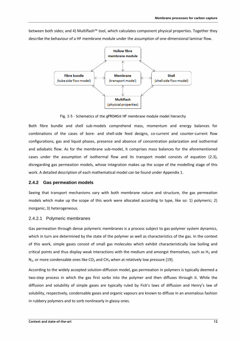
Membrane processes for carbon capture
Context and state-of-the-art 12
between both sides; and 4) ultiflash™ tool, which calculates component physical properties. ogether they
describe the behaviour of a HF membrane module under the assumption of one-dimensional laminar flow.
Fig. 2-5 - Schematics of the gPROMS® HF membrane module model hierarchy
Both fibre bundle and shell sub-models comprehend mass, momentum and energy balances for
combinations of the cases of bore- and shell-side feed designs, co-current and counter-current flow
configurations, gas and liquid phases, presence and absence of concentration polarization and isothermal
and adiabatic flow. As for the membrane sub-model, it comprises mass balances for the aforementioned
cases under the assumption of isothermal flow and its transport model consists of equation (2.3),
disregarding gas permeation models, whose integration makes up the scope of the modelling stage of this
work. A detailed description of each mathematical model can be found under Appendix 1.
2.4.2 Gas permeation models
Seeing that transport mechanisms vary with both membrane nature and structure, the gas permeation
models which make up the scope of this work were allocated according to type, like so: 1) polymeric; 2)
inorganic; 3) heterogeneous.
2.4.2.1 Polymeric membranes
Gas permeation through dense polymeric membranes is a process subject to gas-polymer system dynamics,
which in turn are determined by the state of the polymer as well as characteristics of the gas. In the context
of this work, simple gases consist of small gas molecules which exhibit characteristically low boiling and
critical points and thus display weak interactions with the medium and amongst themselves, such as H2 and
N2, or more condensable ones like CO2 and CH4 when at relatively low pressure [19].
According to the widely accepted solution-diffusion model, gas permeation in polymers is typically deemed a
two-step process in which the gas first sorbs into the polymer and then diffuses through it. While the
diffusion and solubility of simple gases are typically ruled by Fick’s laws of diffusion and enry’s law of
solubility, respectively, condensable gases and organic vapours are known to diffuse in an anomalous fashion
in rubbery polymers and to sorb nonlinearly in glassy ones.

Membrane processes for carbon capture
Context and state-of-the-art 13
Given the different transport mechanisms in play in each case, several sub-models have been developed to
describe gas permeation through dense polymeric membranes, of which the following will be discussed in
detail: 1) molecular; 2) free volume; 3) Flory-Huggins; 4) dual-mode sorption; 5) and partial immobilization.
2.4.2.1.1 Solution-diffusion model [20]
The fundamental concepts of mass transfer are comparable with those of heat conduction and have been
adapted by Fick (1855) to cover quantitative diffusion in an isotropic medium. As a result, the law that
governs the steady-state diffusion of species in the absence of convection is as follows:
(2.8)
Where i is the permeation flux, i the diffusion coefficient, i the concentration and the direction of the
diffusive flow. In an analogous manner, the transport of a gas penetrant through a membrane can be
expressed in terms of a diffusive flow down a concentration gradient across the membrane, which represents
the driving force required for transport. If the diffusion coefficient is assumed constant, integrating the
equation above across a membrane of thickness yields the permeation flux of as follows:
(2.9)
Where i, and i,l are the concentrations of penetrant at the upstream and downstream side of the
membrane, respectively.
Seeing that rubbery polymers exhibit viscous liquid properties and that ideal and simple gases are poorly
soluble in liquid media, according to enry’s law of solubility, the equilibrium concentration of in the gas
phase relates to its partial pressure, i, like so:
(2.10)
In which the solubility coefficient, i, is often independent of concentration or pressure and equal to enry’s
dissolution constant, ,i. The permeation flux can thus be determined via the following expression:
(2.11)
Where i, and i,l are the partial pressures of the penetrant at the upstream and downstream side of the
membrane, respectively. When the downstream penetrant partial pressure is negligible relative to that on
the upstream side, the permeability coefficient, i, can be expressed according to the following equation,
which embodies the solution-diffusion model:
(2.12)
The expression above emphasizes that high permeability coefficients result either from large diffusion
coefficients (e.g. H2), high solubility coefficients (e.g. CO2) or both (e.g. H2O) [21]. The solution-diffusion
model is valid for permeation of simple and ideal gases in rubbery polymers and in glassy polymers at low
Membrane processes for carbon capture
Context and state-of-the-art 14
pressure, assuming that both gas-gas and gas-polymer interactions are negligible, and can be adapted to non-
ideal gas behaviour by replacing partial pressure with fugacity, which can be determined using
thermodynamic equations of state for real gases.
2.4.2.1.2 Molecular model [22]
olecular models are commonly based on the assumption that there exist fluctuating “holes” or
microcavities within the polymer matrix, which can be described by a definite distribution within the polymer
when at equilibrium. Therefore, the diffusion of a penetrant depends greatly upon the concentration of
“holes” large enough to accommodate the penetrant molecule and on the availability of sufficient energy for
a gas molecule to “jump” into a neighbouring “hole”. This concept is supported by the experimentally
observed Arrhenius behaviour of diffusion coefficients, expressed as follows:
ℛ (2.13)
Where ℛ stands for the ideal gas constant, for temperature, ,i for a pre-exponential factor and ,i for
the activation energy of diffusion. One of the first molecular models for diffusion in polymers was proposed
by Meares (1965) and postulates that the primary step in diffusion is governed by the energy required to
separate the polymer chains to form a cylindrical tube through which the penetrant can “ ump” from one
position to another. On the other hand, solubility coefficients exhibit an empirical van’t off relationship with
temperature, expressed as follows:
ℛ (2.14)
In which ,i is a pre-exponential constant and ,i the molar enthalpy of sorption. Seeing that, according to
the solution-diffusion model, permeability is the product of the diffusivity and solubility, combining
equations. (2.15) and (2.16) yields the permeability coefficient as follows:
ℛ
ℛ (2.17)
Where ,i is a pre-exponential constant and P,i the activation energy of permeation, namely the algebraic
sum of ,i and ,i.
2.4.2.1.3 Free volume model [23]
Free volume models differ from molecular models in the fact that rather than considering diffusion as a
thermally activated process, they assume it results from random redistributions of free volume voids within a
polymer matrix. These models are typically based upon the theories of Cohen and Turnbull (1959, 1961)
which describe diffusion as occurring when a molecule can move into a void larger than a critical size, c,i,
formed during the statistical redistribution of free volume within the polymer, f. The probability of
polymer segments of average free volume forming a void larger than the critical size is thought to be
proportional to c,i f . It follows that diffusion is dependent on the availability of an activation
volume and the diffusion coefficient of a species is expressed as follows:

Membrane processes for carbon capture
Context and state-of-the-art 15
(2.18)
This model was originally developed for self-diffusion of a penetrant in an ideal liquid consisting of hard
spheres and is therefore not applicable at temperatures far below the glass transition temperature of the
polymer, where chain motion is virtually non-existent, or at high temperatures where an activation energy
term may be necessary. Another free volume model was conceived by Fujita (1958) to relate the
thermodynamic diffusion coefficient, ,i, to the free volume of the polymer as follows:
(2.19)
In which i and i are temperature-dependent parameters specific to a penetrant-polymer system. f is often
replaced with an equivalent measure of free volume, the fractional free volume of the polymer, . The
relationship between the actual diffusion coefficient and the thermodynamic diffusion one is as follows:
(2.20)
In which i stands for the gas phase activity and i for the volume fraction of penetrant in the polymer.
Seeing that simple gases exhibit relatively low solubilities in polymers, the term i i tends to unity and
both diffusion coefficients are usually considered equivalent. Consequently, the expression which yields the
permeability coefficient according to the free volume model is as follows:
(2.21)
Where
and are temperature-dependent parameters specific to a penetrant-polymer system and the
pre-exponential factor also encompasses the solubility coefficient. However, this model fails to include a
parameter which directly measures penetrant-polymer interactions and lacks the ability to describe size and
shape effects of the penetrant, having been found insufficient in predicting penetrant diffusion coefficients
that are largely independent of concentration due to its overestimation of the critical “hole” size.
2.4.2.1.4 Flory-Huggins model [24]
enry’s law of solubility also holds in case of permeation of condensable gases in rubbery polymers at low
pressures but deviates positively at high pressures, exhibiting the so-called Flory-Huggins swelling behaviour,
as expressed by the following expression, valid for the case of binary systems in the absence of cross-linking
and for a high degree of polymerization:
(2.22)
In which i the saturation vapour pressure and i the Flory-Huggins interaction parameter, which
represents the quality of the penetrant as a solvent for a specific polymer: for i , penetrant-polymer

Membrane processes for carbon capture
Context and state-of-the-art 16
interactions are considered negligible whereas for i they are strong enough to result in significant
dissolution. As for the volume fraction of penetrant in the polymer, it can be determined like so:
(2.23)
Where a represents the amorphous phase volume fraction in the polymer and i the partial molar volume
of the penetrant. Combining the previous two equations and according to enry’s law of solubility, the
equation which yields the solubility coefficient is as follows:
(2.24)
The expression which yields the permeability coefficient throughout the range of penetrant volume fraction
in the polymer is as follows:
(2.25)
In which avg,i represents the average diffusion coefficient across a pressure range. For ideal gases, i is a
convenient measure of activity seeing that the saturation vapour pressure can be estimated using the
Antoine equation, but it can be relaxed for real gas behaviour by replacing partial pressure with fugacity.
However, seeing that at infinite dilution, the penetrant volume fraction can be considered negligible, the
previous expression can be conveniently simplified like so [25]:
(2.26)
Where is the permeability coefficient when the driving force is null, and i is a parameter which
characterizes the pressure dependence of permeability.
2.4.2.1.5 Dual-mode sorption model [20]
Viewing gas permeation in glassy polymers with respect to the solution-diffusion model, the failure of
enry’s solubility law to explain the negative deviation from linear solubility at high pressures can be
explained in terms of the presence of two or more modes for sorption which occur simultaneously. The dual-
mode sorption mechanism was modelled in its final form by Barrer (1958), and Michaels and Vieth (1963)
and postulates that a glassy polymer consists of a continuous chain matrix with dispersed microvoids as a
result from the excess free volume inherent to the non-equilibrium thermodynamic state of the polymer.
Penetrant concentration can therefore be defined in terms of concentration by dissolution in the continuous
chain matrix, i, as well as concentration by sorption in the microvoids, i, according to the following
expression:
(2.27)
Where ,i and ,i are presumed to be in equilibrium, but only ,i is available for diffusion seeing that the
,i consists of completely immobilized gas molecules.

Membrane processes for carbon capture
Context and state-of-the-art 17
he contribution of dissolution to total penetrant concentration is given by enry’s law of solubility and
represents the fraction available for diffusion, whereas the contribution of sorption derives from Langmuir
isotherm, as stated in the equation:
(2.28)
Where ,i represents enry’s dissolution constant, ,i the hole saturation constant, i the Langmuir hole
affinity parameter and i the gas phase partial pressure. Comprising both contributions and assuming the
downstream penetrant partial pressure to be negligible relative to that on the upstream side of the
membrane, the sorption coefficient is as follows:
(2.29)
When the downstream penetrant partial pressure is negligible relative to the upstream side one, a simplified
expression for permeability can be derived as follows [26]:
(2.30)
The dual-mode sorption model is valid for permeation of simple and ideal gases in glassy polymers, assuming
that both gas-gas and gas-polymer interactions are negligible, but can also be adapted to non-ideal gas
behaviour by replacing partial pressure with fugacity.
2.4.2.1.6 Partial immobilization model [20]
The partial immobilization model was first suggested by Petropoulos (1970) and later presented by Paul and
Koros (1976), and proposed the existence of a mobile fraction of Langmuir-mode sorbed gas molecules,
which resulted in the modification of the first Fickian law for diffusion to include separate diffusion
coefficients for Henry mode species, ,i, and for Langmuir mode ones, ,i. The equation which yields the
permeation flux then becomes:
(2.31)
In which both diffusion coefficients are assumed to be concentration independent and the value of ,i is
generally deemed much larger than that of ,i. Introducing a factor , defined as the ratio between ,i and
,i and representative of the mobile fraction of the Langmuir-mode species, the previous expression can be
reformulated like so:
(2.32)
When the downstream penetrant partial pressure is negligible relative to that on the upstream side of the
membrane, a simplified expression for the permeability coefficient can be derived as follows:

Membrane processes for carbon capture
Context and state-of-the-art 18
(2.33)
Null and unit values of factor i are respectively indicative of total and no immobilization of the Langmuir-
mode sorbed gas molecules, whereas intermediate values correspond to partial immobilization and inform
about the effects of upstream pressure on sorption [27]. The dual-mode sorption model with partial
immobilization is widely accepted based on the excellent agreement between the experimental results and
theoretical predictions, along with the simple conceptual description of the process. However, it merely
provides a conceptual reference for data interpretation as it fails to correlate the sorption parameters to
known properties of the gas and the polymer, and the presence of just two distinct sorption modes is an
oversimplification when considering sorption site size distributions.
2.4.2.2 Homogeneous inorganic membranes
Gas permeation through porous inorganic membranes is a process determined by membrane morphology as
well as characteristics of the gas. Porous media can be categorized according to the mean pore diameter as
macroporous (>50 nm), mesoporous (2-50 nm) or microporous (<2 nm), and such distinction is required to
determine the dominant transport mechanism in each case, according to the magnitude of the interactions
between gas and pore walls.
As illustrated in Fig. 2-6, for macro- and mesoporous media, it can be assumed that the void fraction
constitutes a single region under no restriction from the pore wall in which the gas molecules flow freely,
whereas for microporous media there exists an additional layer under strong interaction forces from the pore
wall, consisting of gas molecules sorbed on the surface, which represents the dominant resistance to
permeation. Given the different transport mechanisms in play in each case, of the several models developed
to describe gas permeation, the following will be discussed in detail: 1) pore-flow; and 2) surface diffusion.
Fig. 2-6 - Gas permeation according to pore-flow and surface diffusion models
2.4.2.2.1 Pore-flow model [28]
Gas permeation through porous membranes can be described assuming that the transport through the pores
is far more significant than that in the filled fraction of the material, in which case it can be expressed in
terms of Fickian diffusion:
(2.34)
Where i is the steady-state permeation flux of species through the pores, i is the respective diffusion
coefficient, i is the concentration of in the gas phase and is the direction of the diffusive flow. The
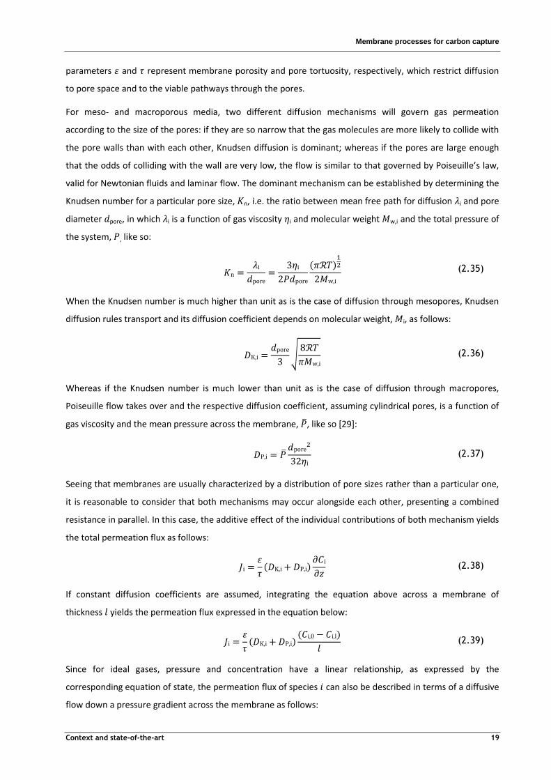
Membrane processes for carbon capture
Context and state-of-the-art 19
parameters and represent membrane porosity and pore tortuosity, respectively, which restrict diffusion
to pore space and to the viable pathways through the pores.
For meso- and macroporous media, two different diffusion mechanisms will govern gas permeation
according to the size of the pores: if they are so narrow that the gas molecules are more likely to collide with
the pore walls than with each other, Knudsen diffusion is dominant; whereas if the pores are large enough
that the odds of colliding with the wall are very low, the flow is similar to that governed by Poiseuille’s law,
valid for Newtonian fluids and laminar flow. The dominant mechanism can be established by determining the
Knudsen number for a particular pore size, n, i.e. the ratio between mean free path for diffusion i and pore
diameter pore, in which i is a function of gas viscosity i and molecular weight w,i and the total pressure of
the system, , like so:
ℛ
(2.35)
When the Knudsen number is much higher than unit as is the case of diffusion through mesopores, Knudsen
diffusion rules transport and its diffusion coefficient depends on molecular weight, i, as follows:
ℛ
(2.36)
Whereas if the Knudsen number is much lower than unit as is the case of diffusion through macropores,
Poiseuille flow takes over and the respective diffusion coefficient, assuming cylindrical pores, is a function of
gas viscosity and the mean pressure across the membrane, , like so [29]:
(2.37)
Seeing that membranes are usually characterized by a distribution of pore sizes rather than a particular one,
it is reasonable to consider that both mechanisms may occur alongside each other, presenting a combined
resistance in parallel. In this case, the additive effect of the individual contributions of both mechanism yields
the total permeation flux as follows:
(2.38)
If constant diffusion coefficients are assumed, integrating the equation above across a membrane of
thickness yields the permeation flux expressed in the equation below:
(2.39)
Since for ideal gases, pressure and concentration have a linear relationship, as expressed by the
corresponding equation of state, the permeation flux of species can also be described in terms of a diffusive
flow down a pressure gradient across the membrane as follows:

Membrane processes for carbon capture
Context and state-of-the-art 20
ℛ
ℛ
(2.40)
The permeability coefficient, i, can thus be expressed according to the following equation, which embodies
the pore-flow model [30]:
ℛ
ℛ (2.41)
The pore-flow model is valid for permeation of ideal gases in porous media, assuming that the gas-pore wall
interaction is negligible, but can be adapted to non-ideal gas behaviour by replacing partial pressure with
fugacity.
2.4.2.2.2 Surface diffusion model [31]
As proposed by Keizer (1988) and later reinforced by Ulhorn (1989), the permeation of a gas species
through the adsorbed phase, also known as surface diffusion, can also be expressed in terms of Fickian
diffusion when corrected according to the Darken equation, as follows:
(2.42)
Where s,i and s,i represent the corrected and zero loading surface diffusion coefficients, respectively, and
i i the thermodynamic correction coefficient, in which i is the partial pressure of at gas phase
and i the concentration of molecules of species sorbed on the surface, also known as loading. Seeing that
surface diffusion is also known to exhibit Arrhenius behaviour, s,i can be expressed like so:
ℛ (2.43)
In which i,s is a pre-exponential factor and s,i is the activation energy of surface diffusion. The expression
which yields the steady-state permeation flux of species then becomes:
(2.44)
In which is the fraction of volume available for surface diffusion. The thermodynamic correction
coefficient can be determined via derivation of the sorption isotherm which best describes the loading of
species over a pressure range. As such, in the event that a Langmuir isotherm accurately describes the
sorption of the species in question, the loading is given according to the following equation:
(2.45)
Where is the loading capacity at saturation and i is the sorption affinity. Conveniently defining a factor
for surface coverage, i i , the thermodynamic correction coefficient is derived as follows [29]:

Membrane processes for carbon capture
Context and state-of-the-art 21
(2.46)
And the equation which yields the permeation flux can be rewritten like so:
(2.47)
If the diffusion coefficient is assumed constant, integrating the equation above across a membrane of
thickness and eliminating the auxiliary variable yields the permeation flux like so:
(2.48)
Resulting in the following expression for the permeability coefficient [32]:
(2.49)
The same reasoning can be applied to other pertinent isotherms so as to obtain different expressions for
permeability. The surface diffusion model is valid for permeation of ideal gases in microporous media but can
be adapted to non-ideal gas behaviour by replacing partial pressure with fugacity.
2.4.2.3 Heterogeneous membranes
Similarly to an electrical circuit, the permeation flux through heterogeneous membranes, such as
asymmetrical or composite ones, can be expressed in terms of equivalent resistance models, of which the
following will be discussed in detail: 1) resistances in series; 2) resistances in parallel; and 3) axwell’s
model.
2.4.2.3.1 Resistances in series [33]
As illustrated in Fig. 2-7, the equivalent resistance to gas permeation through an asymmetrical composite
membrane, eq, can be expressed in terms of the resistances of the membrane and the support, and
consequently in terms of their individual permeances, like so [34]:
(2.50)
In which the indices and correspond to support and membrane, respectively. As a result, the expression
which yields the equivalent permeability, eq, of a supported membrane of thickness eq s m is as
follows:
(2.51)

Membrane processes for carbon capture
Context and state-of-the-art 22
Fig. 2-7 - Schematics of gas permeation through a supported membrane
2.4.2.3.2 Resistances in parallel [29]
As illustrated in Fig. 2-8, the equivalent resistance to gas permeation through a symmetrical composite
membrane, eq, can be expressed in terms of the individual resistances of the disperse phase and the
continuous one, and consequently in terms of their individual permeances, like so:
(2.52)
In which the indices and correspond to disperse and continuous phases, respectively. As a result, the
equation which yields the equivalent permeability of a mixed matrix membrane, eq, is as follows:
(2.53)
Where represents the membrane thickness and d the disperse phase volume fraction.
Fig. 2-8 - Schematics of gas permeation through a mixed matrix membrane
2.4.2.3.3 Maxwell model
For the specific case of mixed matrix membranes in which the disperse phase consists of a dilute suspension
( d 0.2) of particles of filler material, a model derived by Maxwell (1873) for the estimation of the
dielectric properties of composite materials can be used to determine the equivalent permeability, expressed
as follows [35]:
(2.54)
In which the indices and correspond to disperse and continuous phases. However, this model does not
consider effects of particle size, shape or aggregation [36].
2.4.3 Process design
The performance of a membrane process is known to hinge on several factors, of which the following will be
discussed in detail: 1) operating conditions; 2) residence time; 3) pressure ratio; and 4) number of stages.

Membrane processes for carbon capture
Context and state-of-the-art 23
2.4.3.1 Operating conditions
Membrane performance affects that of the process in the sense that high permeability favours recovery,
whereas high selectivity is conductive to great purity. Moreover, both permeability and selectivity
coefficients vary widely with membrane type and are bound to vary differently with temperature and
pressure depending on the transport mechanisms in play.
2.4.3.1.1 Polymeric membranes
According to the solution-diffusion model, which postulates that permeability is the product of diffusivity and
solubility, permeability coefficients are bound to vary differently with operating conditions such as
temperature and pressure, depending on the state of the polymer as well as characteristics of the gas.
Diffusion is typically considered a thermally activated process, which can be described in terms of an
empirical Arrhenius correlation, such as that of equation (2.13), and is therefore enhanced by increasing
temperature [22].
As for the dependence of solubility on temperature in rubbery polymers, it is typically written in terms of an
empirical van’t off relationship and deemed a two-step process, in which the gas molecules first condense
and then polymer matrix rearranges itself to create a molecular scale gap to accommodate the molecule. The
molar enthalpy of sorption corresponds to the algebraic sum of the enthalpy contributions of condensation
and mixing and, whereas for simple gases the mixing enthalpy is positive and dominant, and solubility is
boosted by temperature, for condensable gases and organic vapours the enthalpy for condensation is
negative and dominant and solubility tends to decrease with rising temperature [20].
Assuming constant diffusion, the effect of pressure on permeability is transparent upon observation of the
sorption behaviour of a gas in a polymer. Seeing that the permeation of simple gases in rubbery polymers
presents linear sorption isotherms compliant to enry’s law of solubility, it follows that the permeability
coefficient also increases linearly with rising partial pressure, as illustrated by curve A in Fig. 2-9. However,
for more condensable gases, at sufficiently high pressures, i.e., significant relative to the vapour pressure of
the gas below its critical temperature, and organic vapours, strong deviations can be observed [22].
A sorption isotherm which is concave to the pressure axis, as illustrated by curve B in Fig. 2-9, is characteristic
of penetrant dissolution in glassy polymers and typically described by the dual-mode sorption equation,
which comprises both contributions from enry’s law of solubility, predominant for low pressures, and
Langmuir sorption, which dominates at high pressure. It follows that for glassy polymers, since the diffusion
coefficient remains fairly constant, the dual-mode sorption model predicts a decrease in permeability with
increasing pressure which dampens for high pressures [20].
A sorption isotherm which is convex to the pressure axis and exhibits an inflection point characteristic of
plasticisation, as illustrated by curve C in Fig. 2-9, is characteristic of gas dissolution in rubbery polymers and
typically described by the Flory-Huggins model. For very condensable gases and organic vapours both
diffusion and solubility are strongly enhanced by pressure and, seeing that the parameter which
Membrane processes for carbon capture
Context and state-of-the-art 24
characterizes pressure dependence is typically positive, the permeability coefficient increases with rising
pressure [37].
Fig. 2-9 - Response curves for different sorption behaviours adapted from Dhingra, 1997 [20]
2.4.3.1.2 Inorganic membranes
According to the pore-flow model, the permeation of simple gases through mesopores where Knudsen
diffusion is dominant is enhanced as temperature rises, seeing that the permeability coefficient is
proportional to the square root of temperature. As for macropores, in which Poiseuille flow dominates, since
the viscosity of a gas increases with rising temperature, hindering transport, the corresponding diffusion
coefficient is bound to decrease. It follows that, for simple gases, the permeability coefficient associated to
narrow pores improves with rising temperature, whereas the opposite trend is associated to large pores. On
the other hand, according to the surface diffusion model, the diffusion of condensable gases through
micropores is also a thermally activated process and hence improved by increasing temperature, albeit
slightly offset by the exothermic nature of sorption. The overall effect of temperature on the permeability
coefficient is, however, typically positive [38].
The transport of simple gases through mesopores is not particularly influenced by pressure, whereas in
micropores diffusion rather improves with increasing pressure, seeing that the permeability coefficient is
proportional to the average pressure across the membrane [38]. As for condensable gases, sorption is
impaired by pressure in a manner similar to that of gas permeation through glassy polymeric membranes,
and it follows that the permeability coefficient generally decreases with rising pressure [39].
2.4.3.2 Residence time
Seeing that the permeation flux of component relates to its permeate flow rate and to the membrane area
available for permeation, perm, like so:
(2.55)
Pe
ne
tran
t co
nce
ntr
atio
n
Penetrant pressure
A
B
C
Membrane processes for carbon capture
Context and state-of-the-art 25
It follows that increasing the residence time of the gas in the module, either by increasing the membrane
area, which can be achieved by scaling up its size specifications or by using a larger number of modules in
parallel, or by decreasing the feed flow rate, promotes recovery at the expense of purity [40].
2.4.3.3 Pressure ratio
Flow across the membrane can only occur if the partial pressure of component on the feed side of the
membrane, f,i f,i f, is greater than that on the permeate side of the membrane, p,i p,i p. It follows
that the maximum enrichment achieved by the membrane can never exceed the pressure ratio f p , as the
following equation states [41]:
(2.56)
Consequently, high pressure ratios favour both recovery and purity so that less membrane area is required to
carry out the separation. Pressure ratio can be arranged either by compressing the feed stream or drawing
vacuum on the permeate one, or both at the same time. Although feed compression is more energy-
intensive, it requires less membrane area than permeate vacuum, and is more common in industrial
applications [42].
2.4.3.4 Number of stages
Due to feasibility limitations regarding pressure ratio in industrial processes, typically in the range of 5-15
[41], membrane processes often fail to reach both recovery and purity targets in a single stage, regardless of
the membrane type used. A multi-stage configuration consists of a system of membranes in series, in which
either the permeate stream is recompressed and cooled before being fed to the next stage, enabling further
enrichment to obtain higher purity, in what is known as a membrane cascade; or the retentate stream is fed
to the following stage to facilitate further stripping and promote recovery.
2.4.4 Membrane processes for post-combustion carbon capture
Although the post-combustion implementation of CCS processes is suitable for retrofitting of the majority of
existing fossil-fired power plants, which otherwise have no choice but to keep on venting CO2 to atmosphere,
it also faces many challenges, seeing that power plants produce remarkably large volumes of dilute flue gas
at atmospheric pressure, which translates into low separation driving force, and its high temperature and
saturated water content impair most capture processes [11].
While low partial pressure is of little consequence to amine absorption, keeping up with substantial flow
rates requires very large equipment and intensive heat duty for solvent regeneration, consuming up to ⅓ of
the total steam produced by the plant and increasing the cost of electricity by up to 70 % [43]. The current
efficiency penalty for MEA absorption ranges from 8 to 14 % for different types of power plants [40], and
literature predicts the annual carbon capture process cost for MEA absorption with 90 % recovery in the
range of $40-100/tonCO2 [42], which is still higher than the Clean Coal Research Program (CCRP) target of less
than $40/tonCO2 in the 2020-2025 timeframe and well above the goal of $10/ton by 2035 [44]. Seeing that

Membrane processes for carbon capture
Context and state-of-the-art 26
amine absorption is a mature technology, significant improvements resulting in lower capture costs are
unlikely to happen in the future, urging processes like membrane separation to rise up to the challenge.
Although membrane separation processes incur all of the aforementioned handicaps, several concepts have
been developed to improve separation, of which the following will be discussed in detail: 1) membrane
cascade zoning; 2) recycle processes; 3) cold membrane processes; 4) sweep operation.
2.4.4.1 Membrane cascade zoning
Single-stage membrane processes have been found unable to capture 90 % of the CO2 in flue gas while
producing high-purity CO2 (> 95 mol.%), regardless of the membrane type used [42]. As a result, several
cascade designs, typically ranging from 2 to 4 stages, have been designed to meet the criteria [45], [46].
Seeing that feed streams become progressively richer in CO2 down a cascade, the driving force of separation
gradually becomes less dependent on pressure and therefore less pressure-ratio-limited, as expressed by
equation (2.56). Moreover, given the influence of membrane performance on that of the process, it is
advantageous to divide cascades into zones: a severely pressure-limited stripping zone comprising highly
permeable membranes operating under high pressure ratio, which ensures high recovery with less area
requirements; and an enrichment zone consisting of highly selective membranes operating under low
pressure ratio, which determines product purity [41].
2.4.4.2 Recycle processes
In multi-stage systems, streams with CO2 content much too high to vent out into the atmosphere can be
recycled and introduced into feed streams of previous stages. Although this proves beneficial when the
stream in question is richer in CO2 than the one it is mixed with, improving both recovery and purity, the
reverse dilutes the feed stream, impairing separation. Also, recycling retentate streams enables the recovery
of part of the compression energy by using expanders, while recycling permeate ones entails recompression
[45].
2.4.4.3 Cold membrane processes
Although the molecular model evidences the benefits of temperature on permeability, that on selectivity is
not as obvious. Rather than operating at moderate temperatures so as to reduce cooling costs, cold
membrane processes, i.e., sub-ambient operation enables the tuning of selectivity to exceptional values
while maintaining high permeability when the gas species exhibit sufficiently different parameters [47].
2.4.4.4 Sweep operation
In membrane modules with counter-current flow configurations, introducing a purge/sweep stream
comprising air, inert gas, low pressure water vapour or even decompressed retentate, into the permeate
side, effectively increases the driving force of separation by diluting the permeate. For sufficiently low sweep
flow rates, this approach considerably reduces the membrane area required to achieve separation while the
permeate stream purity remains roughly the same [42].
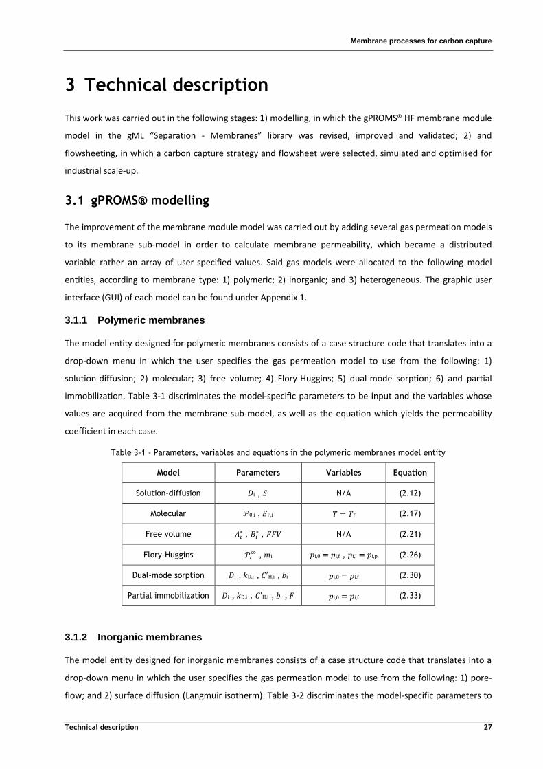
Membrane processes for carbon capture
Technical description 27
3 Technical description
This work was carried out in the following stages: 1) modelling, in which the gPROMS® HF membrane module
model in the gML “Separation - Membranes” library was revised, improved and validated; 2) and
flowsheeting, in which a carbon capture strategy and flowsheet were selected, simulated and optimised for
industrial scale-up.
3.1 gPROMS® modelling
The improvement of the membrane module model was carried out by adding several gas permeation models
to its membrane sub-model in order to calculate membrane permeability, which became a distributed
variable rather an array of user-specified values. Said gas models were allocated to the following model
entities, according to membrane type: 1) polymeric; 2) inorganic; and 3) heterogeneous. The graphic user
interface (GUI) of each model can be found under Appendix 1.
3.1.1 Polymeric membranes
The model entity designed for polymeric membranes consists of a case structure code that translates into a
drop-down menu in which the user specifies the gas permeation model to use from the following: 1)
solution-diffusion; 2) molecular; 3) free volume; 4) Flory-Huggins; 5) dual-mode sorption; 6) and partial
immobilization. Table 3-1 discriminates the model-specific parameters to be input and the variables whose
values are acquired from the membrane sub-model, as well as the equation which yields the permeability
coefficient in each case.
Table 3-1 - Parameters, variables and equations in the polymeric membranes model entity
Model Parameters Variables Equation
Solution-diffusion , N/A (2.12)
Molecular , (2.17)
Free volume
, N/A (2.21)
Flory-Huggins , , (2.26)
Dual-mode sorption , , , (2.30)
Partial immobilization , , , , (2.33)
3.1.2 Inorganic membranes
The model entity designed for inorganic membranes consists of a case structure code that translates into a
drop-down menu in which the user specifies the gas permeation model to use from the following: 1) pore-
flow; and 2) surface diffusion (Langmuir isotherm). Table 3-2 discriminates the model-specific parameters to
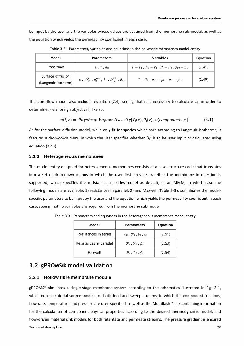
Membrane processes for carbon capture
Technical description 28
be input by the user and the variables whose values are acquired from the membrane sub-model, as well as
the equation which yields the permeability coefficient in each case.
Table 3-2 - Parameters, variables and equations in the polymeric membranes model entity
Model Parameters Variables Equation
Pore-flow , , , , , (2.41)
Surface diffusion
(Langmuir isotherm) ,
, , ,
, , , (2.49)
The pore-flow model also includes equation (2.4), seeing that it is necessary to calculate f,i in order to
determine i via foreign object call, like so:
(3.1)
As for the surface diffusion model, while only fit for species which sorb according to Langmuir isotherms, it
features a drop-down menu in which the user specifies whether i,s
is to be user input or calculated using
equation (2.43).
3.1.3 Heterogeneous membranes
The model entity designed for heterogeneous membranes consists of a case structure code that translates
into a set of drop-down menus in which the user first provides whether the membrane in question is
supported, which specifies the resistances in series model as default, or an MMM, in which case the
following models are available: 1) resistances in parallel; 2) and Maxwell. Table 3-3 discriminates the model-
specific parameters to be input by the user and the equation which yields the permeability coefficient in each
case, seeing that no variables are acquired from the membrane sub-model.
Table 3-3 - Parameters and equations in the heterogeneous membranes model entity
Model Parameters Equation
Resistances in series , , , (2.51)
Resistances in parallel , , (2.53)
Maxwell , , (2.54)
3.2 gPROMS® model validation
3.2.1 Hollow fibre membrane module
gPROMS® simulates a single-stage membrane system according to the schematics illustrated in Fig. 3-1,
which depict material source models for both feed and sweep streams, in which the component fractions,
flow rate, temperature and pressure are user-specified, as well as the ultiflash™ file containing information
for the calculation of component physical properties according to the desired thermodynamic model; and
flow-driven material sink models for both retentate and permeate streams. The pressure gradient is ensured

Membrane processes for carbon capture
Technical description 29
by a control entity which adjusts the pressure in the sweep stream so as to produce the desired value in the
permeate one after undergoing pressure drop throughout the membrane, and the module size specifications
and component permeances are also user-specified. A detailed description of the inputs and outputs of the
HF membrane module model can be found under Appendix 1.
Fig. 3-1 - Topology of a single-stage membrane system with bore- and shell-side feed designs
The gPROMS® HF membrane model was validated against experimental data reported for CO2/N2 separations
by Song et al (2006) [48], Feng and Ivory (2000) [49] and Liu et al (2005) [50], performed using single-stage
membrane systems, and was found to simulate said module with satisfactory accuracy. Unless stated
otherwise, the ultiflash™ file used as a reference for the material source was that of a binary CO2/N2
mixture under ideal gas behaviour and all differential equations pertaining to the membrane module were
solved using the forward finite difference (FFDM) and backward finite difference (BFDM) spacial
discretisation methods as described in Table A1-3 for 50 points. Also, less pertinent information in the form
of tables and figures is available under Appendix A3.
Song et al (2006) reported experimental results using a polyethersulfone (PES) membrane HF module with
bore-side feed design and counter-current flow configuration in a single-stage system with permeate vent to
atmosphere. Table A2-1 comprises the input data for the simulation, and the number of fibres in the bundle,
, was determined to be 3997 using equation (A1.1) since it was not provided in the reference. As illustrated
in Fig. 3-2, the simulated results provide a satisfactory fit to the reported experimental data, seeing that both
permeate and retentate mole fractions and CO2 recovery display similar behaviours throughout the same
stage cut range. However, the model predictions are slightly pessimistic with regard to purity and recovery,
presenting a maximum absolute error of approximately 0.1 for higher stage cuts.
Membrane processes for carbon capture
Technical description 30
Fig. 3-2 - Simulation versus experimental results reported by Song et al (2006) [48]
Feng and Ivory (2000) reported experimental results using a HF membrane module with both bore- and shell-
side feed designs, co- and counter-current flow configurations, and permeate vent to atmosphere and
evacuation under vacuum at 60 cm Hg. Table A2-2 comprises the input data for the simulation, and the fibre
inner diameter, , was assumed equal to the outer one for calculation purposes since it was not provided in
the reference. Fig. 3-3 through Fig. 3-6 depict both simulation and experimental results for bore-side feed
design with the following nomenclature:
ICOA: Co-current flow configuration and permeate vent to atmosphere;
ICCA: Counter-current flow configuration and permeate vent to atmosphere;
ICCV: Counter-current flow configuration and permeate evacuated under vacuum.
Taking into account that scale of the vertical axis is tight throughout, the curves appear quite similar, seeing
that the N2 mole fraction in the retentate is over-predicted for lower stage cuts only by a maximum of ca. 2
%. Nevertheless, membrane performance is particularly optimistic in case of permeate vent to atmosphere
and almost no different from evacuation under vacuum, which is known to be markedly superior. This could
eventually be attributed to the fact that, since the feed pressure is much higher than the permeate one in
both cases, the difference between atmospheric to vacuum evacuation is likely negligible from a numerical
simulation point of view and therefore does not translate into a significative performance boost. Although it
was first considered that the activity model set in the ultiflash™ file might not be appropriate given the
high-pressure feed, simulation with Virial and Redlich-Kwong equations of state led to the exact same results.
0
0,2
0,4
0,6
0,8
1
0,3 0,35 0,4 0,45 0,5
CO
2 m
ole
fra
ctio
n /
C
O2
re
cov
ery
Stage cut
Permeate (exp.)
Permeate (sim.)
Retentate (exp.)
Retentate (sim.)
Recovery (exp.)
Recovery (sim.)

Membrane processes for carbon capture
Technical description 31
Fig. 3-3 - Simulation versus experimental results reported by Feng and Ivory (2000) [49] for N2 mole fraction in
retentate over stage cut for bore-feed side design
Fig. 3-4 - Simulation versus experimental results reported by Feng and Ivory (2000) [49] for N2 mole fraction in
permeate over stage cut for bore-feed side design
Fig. 3-5 - Simulation versus experimental results reported by Feng and Ivory (2000) [49] for retentate flow rate
over N2 mole fraction for bore-feed side design
95
96
97
98
99
100
0,2 0,4 0,6
N2 m
ole
fra
ctio
n i
n
rete
nta
te (
%)
Stage cut
ICOA (exp.)
ICOA (sim.)
ICCA (exp.)
ICCA (sim.)
ICCV (exp.)
ICCV (sim.)
25
35
45
55
65
75
0,2 0,4 0,6
N2 m
ole
fra
ctio
n i
n
pe
rme
ate
(%
)
Stage cut
ICOA (exp.)
ICOA (sim.)
ICCA (exp.)
ICCA (sim.)
ICCV (exp.)
ICCV (sim.)
0
100
200
300
400
500
95 96 97 98 99 100 Re
ten
tate
flo
w r
ate
(sc
cm)
N2 mole fraction in retentate (%)
ICOA (exp.)
ICOA (sim.)
ICCA (exp.)
ICCA (sim.)
ICCV (exp.)
ICCV (sim.)

Membrane processes for carbon capture
Technical description 32
Fig. 3-6 - Simulation versus experimental results reported by Feng and Ivory (2000) [49] for permeate flow rate
over N2 mole fraction for bore-feed side design
On the other hand, Fig. A2-1 through Fig. A2-4 illustrate far too optimistic simulated results for the shell-side
feed design, particularly for lower stage cuts. This discrepancy could eventually be attributed to an
unreported use of a purge stream to force the intended flow configuration, which is known to dilute the
permeate and increase the stage cut, seeing that there is no mention in the reference of how it was
arranged; to the possible occurrence of concentration polarisation, which has been known to happen in shell-
side fed modules for low flow rates, producing a similar effect; or perhaps to fact that membrane permeance
may vary greatly when measured with different feed designs and hence the reported value might not hold in
case of shell-side feed.
Liu et al (2005) reported experimental results using a PEBA membrane HF module with shell-side feed design,
both co- and counter-current flow configurations and permeate vent to atmosphere. Table A2-3 comprises
the input data for the simulation, and the number of fibres in the bundle, , was determined to be 10 using
equation (A1.1). As illustrated in Fig. 3-7 through Fig. 3-11, the simulated performance results provide a
satisfactory fit to the reported experimental data, albeit slightly optimistic, since permeate and retentate
mole fractions display similar behaviours but are over-predicted by a maximum of approximately 10 % for a
given stage cut. However, this seemingly slight discrepancy results in a simulated purity that may exceed
expectations by up to 30 % in case of markedly poor CO2 capture, while far better accuracy is achieved when
high recovery is intended.
60
80
100
120
140
160
25 35 45 55 65 75 Pe
rme
ate
flo
w r
ate
(sc
cm)
N2 mole fraction in permeate (%)
ICOA (exp.)
ICOA (sim.)
ICCA (exp.)
ICCA (sim.)
ICCV (exp.)
ICCV (sim.)

Membrane processes for carbon capture
Technical description 33
Fig. 3-7 - Simulation versus experimental results reported by Liu et al (2005) [50] for CO2 mole fraction in
permeate over stage cut
Fig. 3-8 - Simulation versus experimental results reported by Liu et al (2005) [50] for N2 mole fraction in retentate
over stage cut
Fig. 3-9 - Simulation versus experimental results reported by Liu et al (2005) [50] for permeate rate flow over CO2
mole fraction
30
40
50
60
70
0 0,1 0,2 0,3 0,4 0,5
CO
2 m
ole
fra
ctio
n i
n
pe
rme
ate
(%
)
Stage cut
OCO (exp.)
OCO (sim.)
OCC (exp.)
OCC (sim.)
85
90
95
100
0 0,1 0,2 0,3 0,4 0,5
N2 m
ole
fra
ctio
n i
n
rete
nta
te (
%)
Stage cut
OCO (exp.)
OCO (sim.)
OCC (exp.)
OCC (sim.)
0,04
0,06
0,08
0,1
30 40 50 60 70
Pe
rme
ate
flo
w r
ate
(N
m3∙m
-2∙h
-1)
CO2 mole fraction in permeate (%)
OCO (exp.)
OCO (sim.)
OCC (exp.)
OCC (sim.)

Membrane processes for carbon capture
Technical description 34
Fig. 3-10 - Simulation versus experimental results reported by Liu et al (2005) [50] for CO2 recovery over purity
The HF membrane module was hence adequately validated for operation with stage cuts under ca. 0.5, which
is a typical feasibility limitation. Although there is no clear pattern to the observed discrepancies in this array
of validation cases, the deviations could easily be attributed to parameters not reported in the literature
having been calculated under false assumptions or to membrane permeance having been assessed under
different conditions than those reported for module operation, since permeability may vary widely with
temperature and pressure and permeance differs when assessed for different module configurations.
3.2.2 Permeability models
The gPROMS® permeability models were validated against experimental data reported by several authors
and found to accurately describe gas permeation. For all cases the ultiflash™ file used as a reference for the
material source was that of gas under ideal behaviour. Both input and output validation data can be found
under Appendix A2.
3.2.2.1 Molecular model
Xuezhong and Hägg (2013) [51] reported experimental permeability results of CH4, N2 and CO2 through a
carbon membrane at 2 atm over a temperature range of approximately 295 to 345 K. Table A2-4 contains the
input data for the simulation, and Table A2-5 comprises the results obtained for a temperature of 323 K using
Excel® and gPROMS®, as well as the reported experimental ones, which are illustrated in Fig. A2-5. The
simulated results seem to be in accordance with those calculated using Excel® and with the literature, even
though no approximation error was calculated since the reference values were graphically obtained.
3.2.2.2 Free volume model
Park and Paul (1997) [52] reported experimental permeability results of CH4, N2 and CO2 through various
glassy membranes at 10 atm and 35 °C. Table A2-6 contains the input data for the simulation, and Table A2-7
comprises the results obtained for a fractional free volume of 0.2 using Excel® and gPROMS®, as well as the
reported experimental ones, which are illustrated in Fig. A2-6. The simulated results seem to be in
accordance with those calculated using Excel® and with the literature, even though no approximation error
was calculated since the reference values were graphically obtained. Also, the fact that the results for CO2
0
20
40
60
80
100
30 40 50 60 70
Re
cov
ery
of
CO
2 (
%)
CO2 purity (%)
OCO (exp.)
OCO (sim.)
OCC (exp.)
OCC (sim.)
Membrane processes for carbon capture
Technical description 35
seem poorer than the others is mostly due to the wide dispersion of experimental data, which impairs
graphic reading.
3.2.2.3 Solution-diffusion model
Sanders et al (2012) [53] reported experimental permeability results of CH4, N2 and CO2 through a polyimide
membrane commercially known as HAB-6FDA at 10 atm and 35 °C. Table A2-8 contains the input data for the
simulation, and Table A2-9 comprises the results obtained using Excel® and gPROMS®, as well as the reported
experimental ones. The simulated results concur with those calculated using Excel® and with the literature
and exhibit a maximum relative error of ca. 3.5 %.
3.2.2.4 Dual-mode sorption model
Kanehashi et al (2007) [54] reported experimental results of permeability of CO2 through a PI membrane
commercially known as 6FDA-TeMPD at 10 atm and 35 °C. Table A2-10 contains the input data for the
simulation, and Table A2-11 comprises the results obtained using Excel® and gPROMS®, as well as the
reported experimental ones. The simulated results concur with those calculated using Excel® and with the
literature, exhibiting a relative error of ca. 3.9 %.
3.2.2.5 Partial immobilization model
Tsujita (2003) [55] reported experimental results of permeability of CO2 through PC and PPO membranes at
25 °C and for pressures up to 900 cm Hg. Table A2-12 contains the input data for the simulation, and Table
A2-13 the results obtained for a pressure of 300 cm Hg using Excel® and gPROMS®, as well as the reported
experimental ones, which are illustrated in Fig. A2-7 (curve a). The simulated results seem to be in
accordance with those calculated using Excel® and with the literature, even though no approximation error
was calculated since the reference values were graphically obtained.
3.2.2.6 Flory-Huggins model
Sadrzadeh (2009) [56] reported experimental results of permeability of CH4 and N2 through a
PDMS/polyamide (PA) membrane at 6 bar and 35 °C with permeate atmospheric release. Table A2-14
contains the input data for the simulation, and Table A2-15 the results obtained using Excel® and gPROMS®,
as well as the reported experimental ones. The simulated results seem to be in agreement with those
calculated using Excel® and with the literature, even though no approximation error was calculated since the
reference values were graphically obtained.
3.2.2.7 Pore-flow model
Lira and Paterson (2002) [38] reported experimental results of permeability of CO2, N2 and H2 through
macroporous Al2O3 membranes at 293 K and for pressure gradients up to 1 bar. Table A2-16 contains the
input data for the simulation, and Table A2-17 the results obtained for a pressure gradient of 0.6 bar using
Excel® and gPROMS®, as well as the reported experimental ones, which are illustrated in Fig. A2-8. The
simulated results seem to be in agreement with those calculated using Excel® and to concur with the
Membrane processes for carbon capture
Technical description 36
literature despite the pressure gradient having been used in lieu of the average pressure across the
membrane, seeing that there is no mention of feed nor permeate pressure in the reference.
Shin et al (2005) [57] reported experimental results of permeability of N2 through an array of samples of
macroporous α-Al2O3 membranes at 25 °C and for feed pressures up to 400 kPa. Table A2-18 contains the
input data for the simulation, and Table A2-19 the results obtained for a feed pressure of 200 kPa using
Excel® and gPROMS®, as well as the reported experimental ones, which are illustrated in Fig. A2-9.
The simulated results seem to be in agreement with those calculated using Excel® and to concur with the
literature despite the feed pressure having been used in lieu of the average pressure across the membrane,
as there was no mention of permeate pressure in the reference. Also, the fact that the results for S-D seem
poorer than the others is likely due to its mean pore size being so much larger compared to the other
samples and the contribution of Knudsen diffusion coming close to null, which is not taken into account in
either calculations. Moreover, the discrepancy between Excel® and gPROMS® results mostly derives from gas
viscosity having been determined using the LMNO Engineering gas viscosity [58] calculator and ultiflash™,
respectively.
3.2.2.8 Surface diffusion
Lito et al (2011) [59] reported experimental results of permeance of CO through a zeolite membrane
commercially known as 4A, over a temperature range of 300 to 380 K for 1.2 bar feed pressure and permeate
vent to atmosphere. Table A2-20 contains the input data for the simulation, and Table A2-21 the results
obtained for a temperature of 338 K using Excel® and gPROMS®, as well as the reported experimental ones,
depicted in Fig. A2-10.
Lagorsse et al (2004) [39] reported experimental results of permeability of N2 through a CMS membrane at
303 and 323 K, for a feed pressure range of 1 to 4 bar and permeate vent to atmosphere. Table A2-22
comprises the input data for the simulation, and Table A2-23 the results obtained for a feed pressure of 2 bar
at both temperatures using Excel® and gPROMS®, as well as the reported experimental ones, which are
illustrated in Fig. A2-11.
The simulated results seem to concur with those calculated using Excel® and with the literature, even though
no approximation error was calculated since the reference values were graphically obtained.
3.2.2.9 Resistances in series model
Dingemans et al (2008) [34] reported experimental results of mass transfer coefficients of trichloroethylene
(TCE) through polypropylene (PP)/polyvinylidenedifluoride (PVDF)/PDMS and polyester/ PAN/ PDMS
composite membranes at 30 °C. Table A2-24 contains the individual mass transfer coefficients reported in the
literature, i, from which the permeabilities in Table A2-25, used as input data for the simulation, were
calculated like so:

Membrane processes for carbon capture
Technical description 37
(3.2)
Table A2-26 contains the equivalent permeability results obtained using Excel® and gPROMS®, as well as the
reported experimental ones after processing via equation (3.2). The simulated results are in agreement with
those calculated using Excel® and with the literature and exhibit a maximum relative error of ca. 7.5 %.
3.2.2.10 Resistances in parallel model
Dorosti et al (2011) [60] reported experimental permeability results of CO2, N2 and CH4 through a PSF/PI
MMM at 35 °C and for a range of disperse phase fraction of 0.3 to 0.7. Table A2-27 contains the input data
for the simulation, and Table A2-28 comprises the results obtained using Excel® and gPROMS®, as well as the
reported experimental ones. The simulated results are in accordance with those calculated using Excel® and
with the literature and exhibit a maximum relative error of ca. 14.2 %.
3.2.2.11 Maxwell model
Gheimasi et al (2014) [36] reported experimental permeability results of CO2 through a MMM commercially
known as Sigma-1-Matrimid®5218 at 308 K for disperse phase fractions up to 0.2. Table A2-29 contains the
input data for the simulation, and Table A2-30the results obtained using Excel® and gPROMS®, as well as the
reported experimental ones. The simulated results are in accordance with those calculated using Excel® but
only coincide with the literature ones for significantly low disperse phase fractions, exhibiting a relative error
up to 29.8 %. uch approximation is characteristic of axwell’s model, designed for dilute suspensions, and
consistent with the poor fit reported in the reference, despite the fact that the permeability of the disperse
phase was determined by fitting experimental data to axwell’s model via the least squares method.
3.3 gPROMS® flowsheeting
The flowsheeting stage of this work consisted of selecting a post-combustion implementation of membrane
processes for carbon capture for simulation and optimisation. Unless stated otherwise, all differential
equations pertaining to the membrane modules were solved using FFDM and BFDM spacial discretisation
methods as described in Table A1-3 for 50 points, and all results in the form of tables and figures are
available under Appendix A3.
3.3.1 Simulation and validation
The flowsheet selected was that of a membrane system for carbon capture from flue gas reported by Choi et
al (2013) [46] at pilot-scale, as illustrated in Fig. 3-11. It consists of a 4-stage membrane cascade in which the
retentate of the first stage is vented to the atmosphere while that of the second one is reintroduced to a
dehydration process which precedes the carbon capture one and the remainder are fed to the previous stage
via recycle processes.

Membrane processes for carbon capture
Technical description 38
Fig. 3-11 - Membrane cascade for carbon capture from flue gas reported by Choi et al (2013) [46]
This flowsheet was designed to treat 500 ml/min of flue gas with a CO2 concentration in the range of 10.8 to
11.3 vol.% using HF PES membrane modules with the size specifications listed in Table A3-2 and with a bore-
side feed design and counter-current flow configuration, so as to simultaneously capture 90 % of CO2 and
produce a 99 vol.% CO2-rich product. This reference is the most recent of a series of articles ([48], [61], [62],
[63], [64], [65]), mostly published in Korean, and although some of the size specifications are not explicitly
reported by Choi et al (2013), the gaps of information were filled in with the help of In Seon Kim, who has
kept track of the project from the preparation of the membrane to the operation of the pilot-installation. The
cases described in Table A3-3 were designed, simulated and experimentally performed by Choi et al (2013) to
this end, but only base case 3A succeeded in meeting both criteria.
Given the low range of pressure throughout (<10 bar), the flowsheet gPROMS® simulation was performed on
a molar basis according to the topology illustrated in Fig. A3-2, assuming a feed of 1.339 kmol/h at PTN
conditions containing a CO2 mole fraction of 0.113 for case 3A and of 0.108 for all other cases, and the
ultiflash™ file used as a reference for the material source was that of a binary CO2/N2 mixture under ideal
gas behaviour. Also, all heat exchangers were set to keep each stage feed stream at 25 °C, the usual
temperature for gas permeation experiments, since there is no mention of operating temperature in the
reference, and seeing that the retentate stream of the second stage is fed back upstream of the capture
process with no consequence to the latter, the corresponding recycle process was not simulated.
The membrane permeance of each stage was determined for feed conditions using the fits illustrated in Fig.
A3-1, which in turn were obtained from linear regressions to gas permeation data reported in the same
reference. Moreover, rather than an array of membrane modules in parallel, each stage was simulated as a
single module with the size specifications listed in Table A3-4 and Table A3-5, which were arbitrated so as to
make up the membrane areas reported in the reference while exhibiting the same packing density of 3351
m2/m3 in order to save simulation time and avoid initialisation issues. As illustrated in Table A3-1, this artifice
was previously determined to have insignificant impact on membrane stage performance by simulating the

Membrane processes for carbon capture
Technical description 39
first stage for cases 1 through 3A comprising single and multiple modules and obtaining roughly the same
CO2 recovery in both cases.
As illustrated in Fig. 3-12 through Fig. 3-14, the flowsheet simulation results differ considerably from those
reported by Choi et al (2013), generally exhibiting lower recoveries and higher purities than expected, which
was also observed in the membrane module model validation. While part of the discrepancy in the following
stages can easily be explained by the failure of the first to capture 90 % of the CO2, resulting in a lower flow
rate of purer permeate which drastically alters the dynamics of the rest of the cascade, the poor
performance of the first stage has yet to be faulted, although several explanations have been contemplated.
Fig. 3-12 - Simulation versus experimental results reported by Choi et al (2013) [46] for cases 1 and 2
Fig. 3-13 - Simulation versus experimental results reported by Choi et al (2013) [46] for cases 3A and 3B
Fig. 3-14 - Simulation versus experimental results reported by Choi et al (2013) [46] for case 3C
0%
20%
40%
60%
80%
100%
1 2 3 4 CO
2 R
eco
ve
ry /
Pu
rity
Stage
1 2 3 4
Stage
Recovery (exp.)
Recovery (sim.)
Purity (exp.)
Purity (sim.)
0%
20%
40%
60%
80%
100%
1 2 3 4 CO
2 R
eco
ve
ry /
Pu
rity
Stage
1 2 3 4
Stage
Recovery (exp.)
Recovery (sim.)
Purity (exp.)
Purity (sim.)
0%
20%
40%
60%
80%
100%
1 2 3 4 CO
2 R
eco
ve
ry /
Pu
rity
Stage
Recovery (exp.)
Recovery (sim.)
Purity (exp.)
Purity (sim.)

Membrane processes for carbon capture
Technical description 40
Comparing base cases 1 through 3A to spin-off ones 3B and 3C, the reported pressures for the base cases
seem to consist of target values rather the actual operation ones and may not coincide, which could explain
why the simulated performance parameters of the first stage in the spin-offs are more accurate, but offers
no explanation as to why the simulated results differ from the experimental ones for the rest of the stages.
Also, since the simulation results reported in the reference are also far off the experimental ones for reasons
unknown, that is, the membrane area of each stage had to be manually optimized to meet the desired
performance parameters after their own simulation, against the expectations of the authors, the following
diagnostic tests were performed: 1) gradually decreasing the feed flow rate of the first stage up to ca. 30 %
improved the recovery of the first stage to 90 % but that of the other stages remained far off the
experimental results, as illustrated in Fig. A3-3 through Fig. A3-4, which eliminates the likeliness of the
reported membrane size specifications having been wrongly measured or reported; 2) using equation (2.3)
and the data from Table A3-6 enabled the reverse-calculation of permeance and selectivity for each stage,
which failed to compare to those fitted to reported data by Choi et al (2013), as illustrated in Fig. A3-5
through Fig. A3-7, which indicates that the permeation data might have been wrongly reported.
Although the reverse calculated values are only valid for an ideal flat-sheet membrane under steady-state
conditions, the marked discrepancy offers a possible diagnosis, seeing that the reverse-calculated selectivity
is generally much lower than the linearly fitted one, which accounts for the lower simulated recoveries,
whereas the permeance in the last stage is much higher, which explains the higher simulated purities. This
could perhaps be attributed to permeance having been calculated under different operating conditions, or to
unforeseen membrane plasticization over time, seeing that the installation was said to take very long to
stabilize, and likely much longer than the gas permeation experiments took. Moreover, seeing that the
installation was fed with actual flue gas with an average composition as described in Table A3-7 whereas a
binary CO2/N2 mixture was used in the permeation experiments, the presence of O2 element could be to
blame for part of the discrepancy.
3.3.2 Optimisation and sensitivity analysis
Although the flowsheet reported by Choi et al (2013) was not successfully validated for reasons unknown, its
design was nevertheless optimized in order to minimize the specific cost and energy of carbon capture.
Seeing that the sensitivity analysis performed by Choi et al (2013) covers all of the usual process performance
factors, the flowsheet was instead altered to require less stages and membrane area by introducing a
membrane suited to sub-ambient operation. The membrane in question consists of a HF module comprising
Matrimid® 5218 fibres post-treated with PDMS which were developed for Air Liquide and reported by Liu et
al (2014) [47] to display enhanced low temperature performance for bore-side feed design at a pressure of
6.89 bar for a temperature range of 35 to -40 °C, as illustrated in Fig. 3-15.

Membrane processes for carbon capture
Technical description 41
Fig. 3-15 - CO2/N2 selectivity and CO2 permeance experimental data reported by Liu et al (2014) [47]
The Matrimid®/PDMS membrane was simulated using the gPROMS® HF membrane module model and its
permeability determined via the novel molecular model feature with the parameters in
Table A3-8. The latter were obtained via linear fitting to the permeance data reported for Matrimid®/PDMS,
as illustrated in Fig. A3-8, assuming a 2 µm thick membrane so as to produce the same permeance while
using the module size specifications reported by Choi et al (2013). The temperature range selected was that
between -40 and 50 °C, seeing that the capture process in question follows a dehydration one and therefore
none of the risks associated to typical cryogenic operation apply and that, although a deviation from the
Arrhenius-type behaviour was observed at temperatures lower than -40 °C, there is no reason to believe it
would not hold at 50 °C, the typical feed temperature of flue gas in amine absorption processes.
Since this membrane is more permeable and much more selective than the PES one reported by Choi et al
(2013), simulation determined that the membrane area required for the first stage to attain a recovery of 90
% can be reduced by around 70 % by using Matrimid® at 25 °C, and by approximately 80 % at 50 °C for all
cases, as illustrated in Fig. 3-16. It follows that, as expected, the performance of the first stage benefits from
the introduction of a more permeable membrane at a higher temperature.
Fig. 3-16 - Membrane area requirements to attain 90 % recovery in the first stage
Seeing that compression is preferred to vacuum in an industrial context and that a pressure ratio of 6 is far
more practical than 30, case 1 was used as a reference and the flowsheet was redesigned to consist of only 3
stages, each representing a different zone: 1) a stripping zone at a higher temperature and under a high
pressure ratio; 2) a transition zone under variable conditions; and 3) an enrichment zone, expectedly at a
0
25
50
75
100
125
150
1 2 & 3 Me
mb
ran
e a
rea
(m
2)
Case
PES
Matrimid®, T = 25 °C
Matrimid®, T = 50 °C

Membrane processes for carbon capture
Technical description 42
lower temperature and under a low pressure ratio. The cases described in Table A3-11 were designed to this
end, and
Table A3-12 comprises the simulated results after manual optimisation of membrane area to achieve a
recovery of ca. 90 % at each stage, which suggests that while most cases would produce high-purity CO2, only
case B4 meets the purity criterion set by Choi et al (2013).
Membrane area optimisation was carried out via variation of the module length while keeping the rest of the
size specifications as described in Table A3-4, seeing that the influence of size specifications was previously
determined to be insignificant on the overall performance via simulation of differently sized modules with
the same permeation area, as depicted in Fig. A3-9 and Fig. A3-10, using the information from Table A3-9 and
Table A3-10 for lab- and industrial-sized modules, respectively.
It was found that high pressures and moderate temperatures in the transition zone result in higher purity,
and that cryogenic temperature in the enrichment one is conductive to in ultra-high product purity. Also,
comparing cold membrane process case B4 with reference one 3A, roughly the same purity can be obtained
with only 25 % of the membrane area while attaining an overall recovery of 82.1 % rather than 67.1 %.
To gauge the benefits of the novel membrane system over that proposed by Choi et al (2013), the specific
cost and energy of carbon capture, including downstream compression to 110 bar and cooling to 30 °C [66],
were determined as described under Appendix 4 for cases reported by Choi et al (2013) as well as for those
listed in Table A3-11, and are depicted in Fig. 3-17 and Fig. 3-18. All compression, vacuum and cooling and
equipment were assumed to have the characteristics listed in Table A3-13 through Table A3-15, and the
corresponding duty was obtained via simulation, which was performed using the experimental data in Table
A3-6 for the cases reported in the reference, using each section of the flowsheet at a time so as to ensure its
validity. The downstream compression and cooling were simulated using a series of 11 compressors with a
pressure boost of 10 bar and intermediate cooling to 100 °C.
Fig. 3-17 - Specific cost and energy for the cases reported by Choi et al (2013) [46]
When regarding only the cases which meet the 99 vol.% purity target, B4 was found to be less costly and
energy-intensive as it requires $25.8 and 69.8 kWh to produce a ton of CO2, whereas case 3A demands $41.3
0
20
40
60
80
100
120
1 2 3A 3B 3C
Case
Specific cost ($/tonCO2)
Specific energy (kWh/tonCO2)

Membrane processes for carbon capture
Technical description 43
and 100.0 kWh for the same effect. The annual cost of the carbon capture process was found to decrease
from $5,102 to $3,703 from case 3A to B4, which is mostly attributed to the lesser membrane area but also
to the reduced compression work required. While case 3A is close to reaching the CCRP goal of $40/tonCO2 in
the 2020-2025 timeframe, case B4 is well past it and can potentially be further optimized to reach the
$10/ton by 2035 target.
Considering all of the cases which are expected to produce high-purity CO2, B1 was found to be the least
costly at $25.6 /tonCO2, whereas D2 turned out to be the least energy-intensive at 66.8 kWh/tonCO2. Seeing
that B1 features a high pressure ratio throughout and operates partly above and at ambient temperature,
while D2 features a cold membrane stage under low pressure ratio, it follows that sub-ambient operation
outdoes conventional one from an energetic point of view, and since the specific cost does not differ greatly
between both cases, D2 was deemed most interesting for industrial applications, in which the efficiency
penalty associated to carbon capture is key.
Fig. 3-18 - Specific cost and energy for cases predicted to produce high-purity CO2
Another optimisation effort was the implementation of sweep operation on the second membrane stage by
recirculating decompressed retentate from the first one in order to improve overall recovery and produce
more CO2 with the same membrane area without compromising its purity, rather than decrease area to
maintain recovery constant. Fig. 3-19 illustrates a maximum of performance enhancement for the most
pertinent cases at 5-6 % of retentate recirculation.
Fig. 3-19 - Recovery improvement over sweep operation
25
26
27
28
A3 A4 B1 B2 B3 B4 C4 C5 D2 D3 D4
Sp
eci
fic
cost
($
/to
nC
O2)
Case
65
66
67
68
69
70
71
A3 A4 B1 B2 B3 B4 C4 C5 D2 D3 D4
Sp
eci
fic
en
erg
y
(kW
h/
ton
CO
2)
Case
0,80
0,82
0,84
0,86
0,88
0,90
0 2 4 6 8 10
Ov
era
ll r
eco
ve
ry
Retentate recirculation (%)
B4
B1
D2

Membrane processes for carbon capture
Technical description 44
3.3.3 Industrial scale-up
Assuming that the process performance and specific energy of carbon capture would hold proportionally
from pilot to industrial scale, and considering a fuel-fired power plant such as that reported by Zhao et al
(2008) [40], with the characteristics listed in Table 3-4, it would be possible to implement a post-combustion
membrane carbon capture process based on case D2 with an efficiency penalty as minor as 3.5 %, which is
much lower than that currently attained by MEA absorption.
Table 3-4 - Power plant characteristics reported by Zhao et al (2008) [40]
Fuel type Hard coal
Power output (MW) 1,000
Flue gas flow rate (m3/s) 833
Flue gas temperature (°C) 50
Flue gas CO2 content (mol.%) 13.6
Seeing that running a scaled-up version of case D2 to a factor of 99,960 using that many modules per stage is
borderline infeasible, this case was instead simulated with single module stages with the rather unrealistic
size specifications listed in Table A3-16, which were arbitrated in order to make up the required scaled-up
membrane areas while exhibiting the aforementioned packing density but demanded very slight manual
optimisation to meet pilot-scale performance parameters, which reveals that the influence of size
specifications is perhaps a little more significant at this scale. All equipment specifications were kept the
same as before except for the heat transfer areas, which was scaled-up accordingly, and the expanders
necessary to retentate decompression were simulated as vacuum pumps.
As listed in Table 3-5, the efficiency penalty turned out to be slightly higher than predicted, whereas the cost
of carbon capture was estimated to decrease to $8.0/tonCO2, which is lower than the CCRP target of
$10/tonCO2 by 2035. This can be attributed to estimated equipment cost being proportional to the power of
a decimal, which causes scaling-up to this order of magnitude to be economically advantageous. Moreover,
despite having been found to effectively decrease the specific cost of carbon capture as predicted, sweep
operation turned out to be more energy-intensive, seeing that the energy recovered during retentate
decompression does not make up for the work required to compress a larger volume of gas downstream of
the second stage.
Table 3-5 - Energetic and economic assessment of case D2 at industrial scale
Retentate recirculation (%) 0 6
Specific energy (kWh/tonCO2) 68.3 68.5
Specific cost ($/tonCO2) 8.0 7.7
Energy penalty (%) 3.6 3.8

Membrane processes for carbon capture
Conclusions 45
4 Conclusions
4.1 Goals achieved
In the modelling stage of this work, the membrane module model in gPRO ® g L “ eparation -
embranes” was validated with satisfactory accuracy for stage cuts under ca. .5, predicting membrane
performance with an absolute error of ca. 10 %. This discrepancy was considered to likely derive from
erroneous literature data rather than any major issues concerning numerical simulation. Moreover, its
membrane sub-model was improved to include several gas permeation models as sub-transport models for
different types of membranes, which in turn were successfully validated. As expected, the models associated
to polymeric membranes, more empirical in nature, were found to be more precise than inorganic and
composite ones, which have a more theoretical basis, with a relative error of up to ca. 4 % associated to the
former and of up to approximately 30 % to the latter.
In the flowsheeting stage of this work, a pilot-scale 4-stage membrane cascade for carbon capture from flue
gas comprising recycle processes, designed to capture 90 % of CO2 with a purity of 99 vol.% was simulated
but not successfully validated, seeing that the performance of the first stage was under-predicted by an
absolute maximum of 10 %, which compromised the dynamics of the rest of the cascade despite being
consistent with the discrepancies observed in model validation. Additionally, diagnostic tests enabled the
detection of a possible misreport of permeation data, which literature review led to believe is rather
common. Flowsheet optimisation was thus carried out via introduction of cold membrane processes, which
allowed for the number of stages to be reduced to 3 and lessened the total membrane area by 62 % while
meeting both intended process performance criteria. The specific cost of carbon capture of this design, of
$25.8/tonCO2, was also found to be much lower than that of MEA absorption, of $40-$100/tonCO2, and
inferior than the CCRP goal of $40/tonCO2 in the 2020-2025 timeframe, which confirms the viability of
membrane processes for post-combustion implementations.
Sensitivity analysis confirmed the significance of operating conditions in each zone of the cascade and found
that high temperatures and pressures in the stripping zone are conductive to higher recovery, that high
pressures and moderate temperatures in the transition one result in higher purity, and that cryogenic
temperature in the enrichment zone leads to ultra-high product purity (≥ 99 vol.%). It was also found that, in
these circumstances, sub-ambient operation outdoes conventional one from an energetic point of view,
enabling the production of high-purity (≥ 95 vol.%) CO2 with a specific energy of only 66.8 kWh/tonCO2.
Scale-up of the least energy-intensive design suggested that 90 % of the CO2 emissions of a 1,000 MW fuel-
fired power plant could be treated with a specific cost of only $8.0/tonCO2, which is lower than the CCRP
target of $10/tonCO2 by 2035, and with an efficiency penalty as minor as 3.6 %, which is much lower than
that currently attained by MEA absorption, of 8-14 %. It was also found that, although the introduction of a
Membrane processes for carbon capture
Conclusions 46
sweep stream in the second stage at this scale, comprising 6 % of retentate otherwise vented to atmosphere,
effectively reduces capture cost to $7.7/tonCO2, it also aggravates the energy penalty by 0.2 % and is
therefore not as advantageous as expected.
4.2 Limitations and future work
The main limitations to the work carried out were the lack of explicitness and consistency in published work
concerning membrane processes for carbon capture as well as the shortage of experimental data from multi-
stage membrane systems at any scale. For this reason, more effort should be devoted to obtaining more
accurate experimental data to support model and process simulation and provide a more robust base for
industrial scale-up.
Regarding the gPROMS® membrane model in the context of carbon capture, it would be of interest to further
modify the pertinent model entities to also feature the following gas permeation models: 1) competitive
sorption, as spin-off from dual-mode sorption for better predictive accuracy; 2) configurational diffusion, to
account for exceptional CMS size-sieving; 3) and FSC and SILM facilitated transport, since these novel types of
membranes are expected to outgrow lab-scale stage quite soon. It would also be interesting to extend
beyond gas permeation and explore the modelling of gas-liquid absorption membrane processes, since
conventional absorption for carbon capture is already a mature technology and the use of contactors could
eventually offset its shortcomings.
4.3 Final assessment
It is my opinion that the addition of gas permeation models as local transport ones effectively improves the
accuracy of the highest-level model since the influence of operating conditions on membrane permeability
has been shown to be rather significant but has been erroneously overlooked in most simulation efforts
published thus far.
I also think that the optimistic flowsheet simulation results are relevant in the sense that they demonstrate
that the lack of faith membrane processes in the context of post-combustion carbon capture is unjustified
and that sub-ambient operation might be a gateway into making membrane separation a viable option for
industrial application in fuel-fired power plants.

Membrane processes for carbon capture
References 47
References
[1] International Energy Outlook. Highlights. Energy Information Administration; 2013.
[2] Kost C, Mayer J, Thomsen J, Hartmann N, Senkpiel C, Phillips S, et al. Levelized Cost of Electricity Renewable Energy Technologies. Fraunhofer Institute For Solar Energy Systems ISE; 2013.
[3] Pires JCM, Martins FG, Alvim-Ferraz MCM, Simões M. Recent developments on carbon capture and storage: An overview. Chemical Engineering Research and Design. 2011;89:1446-60.
[4] Figueroa JD, Fout T, Plasynski S, McIlvried H, Srivastava RD. Advances in CO2 capture technology—The U.S. Department of Energy's Carbon Sequestration Program. International Journal of Greenhouse Gas Control. 2008;2:9-20.
[5] Czyperek M, Zapp P, Bouwmeester HJM, Modigell M, Ebert K, Voigt I, et al. Gas separation membranes for zero-emission fossil power plants: MEM-BRAIN. Journal of Membrane Science. 2010;359:149-59.
[6] Peters L, Hussain A, Follmann M, Melin T, Hägg MB. CO2 removal from natural gas by employing amine absorption and membrane technology—A technical and economical analysis. Chemical Engineering Journal. 2011;172:952-60.
[7] Rufford TE, Smart S, Watson GCY, Graham BF, Boxall J, Diniz da Costa JC, et al. The removal of CO2 and N2 from natural gas: A review of conventional and emerging process technologies. Journal of Petroleum Science and Engineering. 2012;94–95:123-54.
[8] Bergel M, Tierno I. Sweetening technologies—a look at the whole picture. 24th World Gas Conference. International Gas Union, Buenos Aires, Argentina2009. p. 1–17.
[9] Marriott JI. Detailed Modelling and Optimal Design of Membrane Separation Systems: University of London; 2001.
[10] Chen HZ, Thong Z, Li P, Chung T-S. High performance composite hollow fiber membranes for CO2/H2 and CO2/N2 separation. International Journal of Hydrogen Energy. 2014;39:5043-53.
[11] Budd PM, McKeown NB, Fritsch D. Free volume and intrinsic microporosity in polymers. Journal of Materials Chemistry. 2005;15:1977-86.
[12] Hoek EMV, Tarabara VV. Encyclopedia of Membrane Science and Technology: Wiley; 2013.
[13] Ramasubramanian K, Ho WSW. Recent developments on membranes for post-combustion carbon capture. Current Opinion in Chemical Engineering. 2011;1:47-54.
[14] Kong C, Lu J, Yang J, Wang J. Preparation of silicalite-1 membranes on stainless steel supports by a two-stage varying-temperature in situ synthesis. Journal of Membrane Science. 2006;285:258-64.
[15] Boon J, Pieterse JAZ, Dijkstra JW, van Sint Annaland M. Modelling and systematic experimental investigation of mass transfer in supported palladium-based membrane separators. International Journal of Greenhouse Gas Control. 2012;11, Supplement:S122-S9.
[16] Shahkaramipour N, Adibi M, Seifkordi AA, Fazli Y. Separation of CO2/CH4 through alumina-supported geminal ionic liquid membranes. Journal of Membrane Science. 2014;455:229-35.
[17] Rezakazemi M, Ebadi Amooghin A, Montazer-Rahmati MM, Ismail AF, Matsuura T. State-of-the-art membrane based CO2 separation using mixed matrix membranes (MMMs): An overview on current status and future directions. Progress in Polymer Science. 2014;39:817-61.
[18] Wey M-Y, Tseng H-H, Chiang C-k. Improving the mechanical strength and gas separation performance of CMS membranes by simply sintering treatment of α-Al2O3 support. Journal of Membrane Science. 2014;453:603-13.
[19] Baird DG, Collias DI. Polymer Processing: Principles and Design: Wiley; 2014.
[20] Dhingra SS. Mixed Gas Transport Study Through Polymeric Membranes: A Novel Technique. Blacksburg, Virginia: Faculty of the Virginia Polytechnic Institute and State University; 1997.
[21] Mark HF. Encyclopedia of Polymer Science and Technology. John Wiley & Sons, Inc.
[22] Freeman B, Yampolskii Y, Pinnau I. Materials Science of Membranes for Gas and Vapor Separation: Wiley; 2006.
[23] Thran A, Kroll G, Faupel F. Correlation between fractional free volume and diffusivity of gas molecules in glassy polymers. Journal of Polymer Science Part B: Polymer Physics. 1999;37:3344-58.
[24] Lin H, Freeman BD. Gas solubility, diffusivity and permeability in poly(ethylene oxide). Journal of Membrane Science. 2004;239:105-17.

Membrane processes for carbon capture
References 48
[25] Ribeiro Jr CP, Freeman BD. Carbon dioxide/ethane mixed-gas sorption and dilation in a cross-linked poly(ethylene oxide) copolymer. Polymer. 2010;51:1156-68.
[26] Li P, Chung TS, Paul DR. Temperature dependence of gas sorption and permeation in PIM-1. Journal of Membrane Science. 2014;450:380-8.
[27] Koros WJ, Paul DR, Rocha AA. Carbon dioxide sorption and transport in polycarbonate. Journal of Polymer Science: Polymer Physics Edition. 1976;14:687-702.
[28] Jareman F. Properties and Modelling of MFI membranes. Lulea, Sweeden: Lulea University of Technology; 2004.
[29] Marković A Stoltenberg D Enke D Schlünder EU Seidel-Morgenstern A. Gas permeation through porous glass membranes: Part I. Mesoporous glasses—Effect of pore diameter and surface properties. Journal of Membrane Science. 2009;336:17-31.
[30] Keizer K, Uhlhorn RJR, Vuren RJv, Burggraaf AJ. Gas separation mechanisms in microporous modified γ-al2o3 membranes. Journal of Membrane Science. 1988;39:285-300.
[31] A.J. Burggraaf LC. Fundamentals of Inorganic Membrane Science and Technology. Elsevier Science B. V.; 1996.
[32] Lim Y-I, Bhatia SK, Nguyen TX, Nicholson D. Prediction of carbon dioxide permeability in carbon slit pores. Journal of Membrane Science. 2010;355:186-99.
[33] Li P, Chen HZ, Chung T-S. The effects of substrate characteristics and pre-wetting agents on PAN–PDMS composite hollow fiber membranes for CO2/N2 and O2/N2 separation. Journal of Membrane Science. 2013;434:18-25.
[34] Dingemans M, Dewulf J, Braeckman L, Van Langenhove H, Friess K, Hynek V, et al. Mass transfer characteristics for VOC permeation through flat sheet porous and composite membranes: The impact of the different membrane layers on the overall membrane resistance. Journal of Membrane Science. 2008;322:234-42.
[35] Chung T-S, Jiang LY, Li Y, Kulprathipanja S. Mixed matrix membranes (MMMs) comprising organic polymers with dispersed inorganic fillers for gas separation. Progress in Polymer Science. 2007;32:483-507.
[36] Gheimasi KM, Peydayesh M, Mohammadi T, Bakhtiari O. Prediction of CO2/CH4 permeability through Sigma-1–Matrimid®5218 MMMs using the Maxwell model. Journal of Membrane Science. 2014;466:265-73.
[37] Merkel TC, Bondar VI, Nagai K, Freeman BD, Pinnau I. Gas sorption, diffusion, and permeation in poly(dimethylsiloxane). Journal of Polymer Science Part B: Polymer Physics. 2000;38:415-34.
[38] Lira HdL, Paterson R. New and modified anodic alumina membranes: Part III. Preparation and characterisation by gas diffusion of 5 nm pore size anodic alumina membranes. Journal of Membrane Science. 2002;206:375-87.
[39] Lagorsse S, Magalhães FD, Mendes A. Carbon molecular sieve membranes: Sorption, kinetic and structural characterization. Journal of Membrane Science. 2004;241:275-87.
[40] Zhao L, Riensche E, Menzer R, Blum L, Stolten D. A parametric study of CO2/N2 gas separation membrane processes for post-combustion capture. Journal of Membrane Science. 2008;325:284-94.
[41] Huang Y, Merkel TC, Baker RW. Pressure ratio and its impact on membrane gas separation processes. Journal of Membrane Science. 2014;463:33-40.
[42] Merkel TC, Lin H, Wei X, Baker R. Power plant post-combustion carbon dioxide capture: An opportunity for membranes. Journal of Membrane Science. 2010;359:126-39.
[43] Yang H, Xu Z, Fan M, Gupta R, Slimane RB, Bland AE, et al. Progress in carbon dioxide separation and capture: A review. Journal of Environmental Sciences. 2008;20:14-27.
[44] Carbon Capture Technology Program Plan. United States Department of Energy; 2013.
[45] Zhao L, Riensche E, Weber M, Stolten D. Cascaded Membrane Processes for Post-Combustion CO2 Capture. Chemical Engineering & Technology. 2012;35:489-96.
[46] Choi S-H, Kim J-H, Lee Y. Pilot-scale multistage membrane process for the separation of CO2 from LNG-fired flue gas. Separation and Purification Technology. 2013;110:170-80.
[47] Liu L, Sanders ES, Kulkarni SS, Hasse DJ, Koros WJ. Sub-ambient temperature flue gas carbon dioxide capture via Matrimid® hollow fiber membranes. Journal of Membrane Science. 2014;465:49-55.
[48] Song I, Ahn H, Y.Lee, Jeon H, Y.Lee, Kim JH, et al. Carbon dioxide separation by hollow fibre membrane of polyethersulfone: Comparison of experimental results with numerical analysis data. Membrane Journal 16. 2006:252–8.
[49] Feng X, Ivory J. Development of hollow fiber membrane systems for nitrogen generation from combustion exhaust gas: Part I. Effects of module configurations. Journal of Membrane Science. 2000;176:197-207.

Membrane processes for carbon capture
References 49
[50] Liu L, Chakma A, Feng X. CO2/N2 Separation by Poly(Ether Block Amide) Thin Film Hollow Fiber Composite Membranes. Industrial & Engineering Chemistry Research. 2005;44:6874-82.
[51] He X, Hägg M-B. Hollow fiber carbon membranes: From material to application. Chemical Engineering Journal. 2013;215–216:440-8.
[52] Park JY, Paul DR. Correlation and prediction of gas permeability in glassy polymer membrane materials via a modified free volume based group contribution method. Journal of Membrane Science. 1997;125:23-39.
[53] Sanders DF, Smith ZP, Ribeiro Jr CP, Guo R, McGrath JE, Paul DR, et al. Gas permeability, diffusivity, and free volume of thermally rearranged polymers based on 3 3′-dihydroxy-4 4′-diamino-biphenyl (HAB) and 2 2′-bis-(3,4-dicarboxyphenyl) hexafluoropropane dianhydride (6FDA). Journal of Membrane Science. 2012;409–410:232-41.
[54] Kanehashi S, Nakagawa T, Nagai K, Duthie X, Kentish S, Stevens G. Effects of carbon dioxide-induced plasticization on the gas transport properties of glassy polyimide membranes. Journal of Membrane Science. 2007;298:147-55.
[55] Tsujita Y. Gas sorption and permeation of glassy polymers with microvoids. Progress in Polymer Science. 2003;28:1377-401.
[56] Sadrzadeh M, Shahidi K, Mohammadi T. Effect of operating parameters on pure and mixed gas permeation properties of a synthesized composite PDMS/PA membrane. Journal of Membrane Science. 2009;342:327-40.
[57] Shin DW, Hyun SH, Cho CH, Han MH. Synthesis and CO2/N2 gas permeation characteristics of ZSM-5 zeolite membranes. Microporous and Mesoporous Materials. 2005;85:313-23.
[58] Edwards K. LMNO Engineering, Research, and Software, Ltd. p. LMNO Engineering Gas Viscosity Calculator.
[59] Lito PF, Santiago AS, Cardoso SP, Figueiredo BR, Silva CM. New expressions for single and binary permeation through zeolite membranes for different isotherm models. Journal of Membrane Science. 2011;367:21-32.
[60] Dorosti F, Omidkhah MR, Pedram MZ, Moghadam F. Fabrication and characterization of polysulfone/polyimide–zeolite mixed matrix membrane for gas separation. Chemical Engineering Journal. 2011;171:1469-76.
[61] Kim J-H, Sohn W-I, Choi S-H, Lee S-B. Preparation of asymmetric polyethersulfone hollow fiber membranes for flue gas separation. Membrane Journal. 2005;15:147-56.
[62] Choi S-H, Kim J-H, Kim B-S, Lee S-B. Multi-stage membrane process for CO2 separation from flue gas using PES hollow fiber membrane modules. Membrane Journal. 2005;15:310-9.
[63] Song I, Ahn H, Lee Y, Jeon H, Lee Y, Kim J-H, et al. Analysis of carbon dioxide separation with countercurrent flow in hollow fiber membrane by numerical analysis. Membrane Journal. 2006;16:252-8.
[64] Song I, Ahn H, Jeon H, Joung H-K, Lee Y, Kim J-H, et al. Carbon dioxide separation by hollow fibermembrane of polyethersulfone: Comparison of experimental results with numerical analysis data. Membrane Journal. 2007;17:134-9.
[65] Song I, Ahn H, Jeon H, Jeong H-K, Lee Y, Choi S-H, et al. Optimal design of multiple stage membrane process for carbon dioxide separation. Desalination. 2008;234:307-15.
[66] Zhao L, Riensche E, Blum L, Stolten D. How gas separation membrane competes with chemical absorption in postcombustion capture. Energy Procedia. 2011;4:629-36.
[67] Ivory J, Feng X, Kovacik G. Development of hollow fiber membrane systems for nitrogen generation from combustion exhaust gas: Part II: Full-scale module test and membrane stability. Journal of Membrane Science. 2002;202:195-204.
[68] Smith RM. Chemical Process: Design and Integration: Wiley; 2005.
[69] Mignard D. Correlating the chemical engineering plant cost index with macro-economic indicators. Chemical Engineering Research and Design. 2014;92:285-94.

Membrane processes for carbon capture
Appendix 1 50
Appendix 1 gPROMS® model description
A1.1 Hollow fibre membrane module model
Table A1-1 and Table A1-2 comprise the inputs and outputs of the original HF membrane module model for
bore- and shell-side feed design cases, respectively, and Table A1-3 lists the spacial discretisation methods
employed in each case for each sub-model.
Table A1-1 - HF membrane module model input and output data for the bore-side feed design case
Model Input Output
Fibre bundle
Feed flow rate,
Feed composition,
Feed pressure,
Tube side partial pressure,
Shell
Sweep flow rate,
Sweep composition,
Sweep pressure,
Shell side partial pressure,
Membrane
Permeance,
Tube side partial pressure,
Shell side partial pressure,
Component flux,
Membrane
module
Size specifications
o Fibre bundle length,
o Fibre inner diameter,
o Fibre outer diameter,
o Number of fibres,
o Shell diameter,
Component flux,
Permeation area,
Retentate composition,
Retentate pressure,
Permeate composition,
Permeate pressure,
Table A1-2 - HF membrane module model input and output data for the shell-side feed design case
Model Input Output
Fibre bundle
Feed flow rate,
Feed composition,
Feed pressure,
Tube side partial pressure,
Shell
Sweep flow rate,
Sweep composition,
Sweep pressure,
Shell side partial pressure,
Membrane
Permeance,
Tube side partial pressure,
Shell side partial pressure,
Component flux,
Membrane
module
Size specifications
o Fibre bundle length,
o Fibre inner diameter,
o Fibre outer diameter,
o Number of fibres,
o Shell diameter,
Component flux,
Permeation area,
Retentate composition,
Retentate pressure,
Permeate composition,
Permeate pressure,

Membrane processes for carbon capture
Appendix 1 51
Table A1-3 - HF membrane module spacial discretisation methods
Sub-model Fibre bundle Shell
Feed design Flow configuration Axial, Shifted axial, Axial, Shifted axial,
Tube-side
Co-current BFDM FFDM BFDM FFDM
Counter-current BFDM FFDM FFDM BFDM
Shell-side
Co-current BFDM FFDM BFDM FFDM
Counter-current FFDM BFDM BFDM FFDM
A1.2 Membrane sub-model
Equations (A1.1) through (A1.8) describe the membrane sub-model.
Average surface area for permeation, perm:
(A1.1)
Component flow rate, :
(A1.2)
Partial pressures, tube and shell :
(A1.3)
(A1.4)
Steady-state molar flux for bore-side feed case:
(A1.5)
Energy flow rate, (calculated via foreign object call) for bore-side feed case:
(A1.6)
Steady-state molar flux for shell-side feed case:
(A1.7)
Energy flow rate, (calculated via foreign object call) for shell-side feed case:
(A1.8)

Membrane processes for carbon capture
Appendix 1 52
A1.3 Fibre bundle sub-model
Equations (A1.9) through (A1.33) describe the fibre bundle sub-model.
Fibre bundle inner surface area, inner, bundle:
(A1.9)
Fibre cross section area, area, tube:
(A1.10)
Concentration, :
(A1.11)
Concentration polarisation at the interface according to the bulk model:
(A1.12)
Concentration polarisation at the interface according to the stagnant film model:
(A1.13)
Fibre flux for purely convective flow, bre :
(A1.14)
Frictional parameter, :
(A1.15)
Energy flow rate, :
(A1.16)
Energy hold-up, :
(A1.17)
The following properties are calculated via foreign object call:
Density, :
(A1.18)
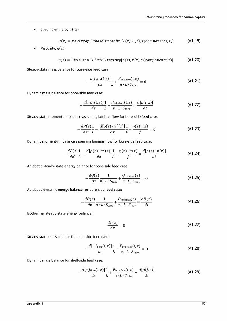
Membrane processes for carbon capture
Appendix 1 53
Specific enthalpy, :
(A1.19)
Viscosity, :
(A1.20)
Steady-state mass balance for bore-side feed case:
(A1.21)
Dynamic mass balance for bore-side feed case:
(A1.22)
Steady-state momentum balance assuming laminar flow for bore-side feed case:
(A1.23)
Dynamic momentum balance assuming laminar flow for bore-side feed case:
(A1.24)
Adiabatic steady-state energy balance for bore-side feed case:
(A1.25)
Adiabatic dynamic energy balance for bore-side feed case:
(A1.26)
Isothermal steady-state energy balance:
(A1.27)
Steady-state mass balance for shell-side feed case:
(A1.28)
Dynamic mass balance for shell-side feed case:
(A1.29)

Membrane processes for carbon capture
Appendix 1 54
Steady-state momentum balance assuming laminar flow for shell-side feed case:
(A1.30)
Dynamic momentum balance assuming laminar flow for shell-side feed case:
(A1.31)
Adiabatic steady-state energy balance for shell-side feed case:
(A1.32)
Adiabatic dynamic energy balance for shell-side feed case:
(A1.33)
A1.4 Shell sub-model
Equations (A1.34) through (A1.58) describe the shell sub-model.
Fibre bundle outer surface area, outer,bundle:
(A1.34)
Fibre bundle cross section area, area, bundle:
(A1.35)
Shell cross section area, area, shell:
(A1.36)
Parameter :
(A1.37)
Equivalent diameter, eq:
(A1.38)
Frictional parameter, :
(A1.39)

Membrane processes for carbon capture
Appendix 1 55
Concentration, :
(A1.40)
Concentration polarisation at the interface according to the bulk model:
(A1.41)
Concentration polarisation at the interface according to the stagnant film model:
(A1.42)
Fibre flux for purely convective flow, bre :
(A1.43)
Energy flow rate, :
(A1.44)
Energy hold-up, :
(A1.45)
Density, , specific enthalpy, , and viscosity, , are calculated via foreign object call via equations
(A1.18) through (A1.20).
Steady-state mass balance for bore-side feed case:
(A1.46)
Dynamic mass balance for bore-side feed case:
(A1.47)
Steady-state momentum balance assuming laminar flow for bore-side feed case:
(A1.48)
Dynamic momentum balance assuming laminar flow for bore-side feed case:
(A1.49)

Membrane processes for carbon capture
Appendix 1 56
Adiabatic steady-state energy balance for bore-side feed case:
(A1.50)
Adiabatic dynamic energy balance for bore-side feed case:
(A1.51)
Isothermal steady-state energy balance:
(A1.52)
Steady-state mass balance for shell-side feed case:
(A1.53)
Dynamic mass balance for shell-side feed case:
(A1.54)
Steady-state momentum balance assuming laminar flow for shell-side feed case:
(A1.55)
Dynamic momentum balance assuming laminar flow for shell-side feed case:
(A1.56)
Adiabatic steady-state energy balance for shell-side feed case:
(A1.57)
Adiabatic dynamic energy balance for shell-side feed case:
(A1.58)
A1.5 Permeability sub-models
Fig. A1-1 through Fig. A1-11 illustrate the GUI of each permeability model upon double-clicking on the
membrane sub-model in the topology tab.

Membrane processes for carbon capture
Appendix 1 57
Fig. A1-1 - GUI of the polymeric membrane model entity featuring the molecular model
Fig. A1-2 - GUI of the polymeric membrane model entity featuring the free volume model
Fig. A1-3 - GUI of the polymeric membrane model entity featuring the solution-diffusion model

Membrane processes for carbon capture
Appendix 1 58
Fig. A1-4 - GUI of the polymeric membrane model entity featuring the dual sorption model
Fig. A1-5 - GUI of the polymeric membrane model entity featuring the partial immobilization model
Fig. A1-6 - GUI of the polymeric membrane model entity featuring the Flory-Huggins model

Membrane processes for carbon capture
Appendix 1 59
Fig. A1-7 - GUI of the inorganic membrane model entity featuring the pore-flow model
Fig. A1-8 - GUI of the inorganic membrane model entity featuring the surface diffusion model
Fig. A1-9 - GUI of the heterogeneous membrane model entity featuring the resistances in series model
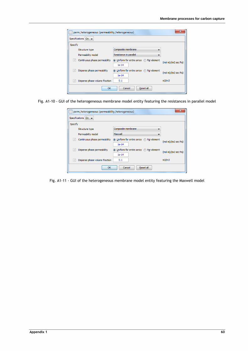
Membrane processes for carbon capture
Appendix 1 60
Fig. A1-10 - GUI of the heterogeneous membrane model entity featuring the resistances in parallel model
Fig. A1-11 - GUI of the heterogeneous membrane model entity featuring the Maxwell model

Membrane processes for carbon capture
Appendix 2 61
Appendix 2 gPROMS® model validation
A2.1 Hollow fibre membrane module model
Table A2-1 and Table A2-2 comprise the input data for simulation as reported by Song et al (2006) and by
Feng and Ivory (2000), respectively.
Table A2-1 - Input data reported by Song et al (2006) [48]
Table A2-2 - Input data reported by Feng and Ivory (2000) [49]
( / )CO2 (GPU) 57.9 45
( / )N2 (GPU) 1.3 (cm) 105
CO2 (%) 18.3 (μm) 165
N2 (%) 81.7 (cm2) 245
f (MPa) 2.07 (in) 3/16
(°C) 22
Fig. A2-1 through Fig. A2-4 illustrate the experimental and simulated results reported by Feng and Ivory
(2000) for shell-side feed design with different combinations of flow configuration and permeate discharge,
identified as follows:
OCOA: co-current flow configuration, permeate vent to atmosphere;
OCCA: counter-current flow configuration, permeate vent to atmosphere;
OCCV: counter-current flow configuration, permeate evacuated under vacuum.
(mol∙m-2∙s-1∙Pa-1) 1.58E-08 (cm) 45
(mol∙m-2∙s-1∙Pa-1) 9.89E-10 (μm) 4
(%) 33 (μm) 2
(%) 67 (cm2) 2.26
(kPa) 591.7 (mm) 50.8
(°C) 25

Membrane processes for carbon capture
Appendix 2 62
Fig. A2-1 - Simulation versus experimental results reported by Feng and Ivory (2000) [49] for N2 mole fraction in
retentate over stage cut for shell-feed side design
Fig. A2-2 - Simulation versus experimental results reported by Feng and Ivory (2000) [49] for N2 mole fraction in
permeate over stage cut for shell-feed side design
Fig. A2-3 - Simulation versus experimental results reported by Feng and Ivory (2000) [49] for retentate flow rate
over N2 mole fraction for shell-feed side design
95
96
97
98
99
100
0,2 0,4 0,6
N2 m
ole
fra
ctio
n i
n
rete
nta
te (
%)
Stage cut
OCOA (exp.)
OCOA (sim.)
OCCA (exp.)
OCCA (sim.)
OCCV (exp.)
OCCV (sim.)
20
25
30
35
40
45
50
55
0,2 0,4 0,6
N2 m
ole
fra
ctio
n i
n
pe
rme
ate
(%
)
Stage cut
OCOA (exp.)
OCOA (sim.)
OCCA (exp.)
OCCA (sim.)
OCCV (exp.)
OCCV (sim.)
0
50
100
150
200
250
95 96 97 98 99 100 Re
ten
tate
flo
w r
ate
(sc
cm)
N2 mole fraction in retentate (%)
OCOA (exp.)
OCOA (sim.)
OCCA (exp.)
OCCA (sim.)
OCCV (exp.)
OCCV (sim.)
Membrane processes for carbon capture
Appendix 2 63
Fig. A2-4 - Simulation versus experimental results reported by Feng and Ivory (2000) [49] for permeate flow rate
over N2 mole fraction for shell-feed side design
Table A2-3 comprises the input data for simulation as reported by Liu et al (2005).
Table A2-3 - Input data reported by Liu et al (2005) [50]
(GPU) 48.2 (cm) 22
(GPU) 1.7 (μm) 700
(%) 15.3 (μm) 500
(%) 84.7 (cm2) 43.5
(kPa) 790 (m) 0.0064
(°C) 23
A2.2 Permeability models
Table A2-4 contains the input data for the simulation as reported by Xuezhong and Hägg (2013) [51], and
Table A2-5 comprises the results obtained for a temperature of 323 K using Excel® and gPROMS®, as well as
the reported experimental ones, which are illustrated in Fig. A2-5.
Table A2-4 - Molecular model parameters reported by Xuezhong and Hägg (2013) [50]
Species, (Barrer) (kJ∙mol-1)
CO2 1049.4 2.4
N2 133.6 6.8
CH4 5602.7 18.2
40
50
60
70
80
90
100
20 25 30 35 40 45 50 55 60 Pe
rme
ate
flo
w r
ate
(sc
cm)
N2 mole fraction in permeate (%)
OCOA (exp.)
OCOA (sim.)
OCCA (exp.)
OCCA (sim.)
OCCV (exp.)
OCCV (sim.)

Membrane processes for carbon capture
Appendix 2 64
Table A2-5 - Permeability computed according to the molecular model for = 323 K
Species, (mol∙m∙m-2∙s-1∙Pa-1)
Excel® gPROMS® Reference [51]
CO2 1.44E-13 1.44E-13 1.42E-13
N2 3.54E-15 3.55E-15 3.69E-15
CH4 2.12E-15 2.11E-15 2.03E-15
Fig. A2-5 - Experimental permeability results reported by Xuezhong and Hägg (2013) [50]
Table A2-6 contains the input data for the simulation as reported by Park and Paul (1997) [52], and Table A2-
7 comprises the results obtained for a fractional free volume of 0.2 using Excel® and gPROMS®, as well as the
reported experimental ones, which are illustrated in Fig. A2-6.
Table A2-6 - Free volume parameters reported by Park and Paul (1997) [52]
Species, (Barrer)
CH4 114 0.967
N2 112 0.914
CO2 1750 0.860

Membrane processes for carbon capture
Appendix 2 65
Table A2-7 - Permeability computed according to the free volume model for = 0.2
Species, (mol∙m∙m-2∙s-1∙Pa-1)
Excel® gPROMS® Reference [52]
CH4 3.03E-16 3.03E-16 3.01E-16
N2 3.88E-16 3.88E-16 3.35E-16
CO2 7.95E-15 7.95E-15 6.70E-15
Fig. A2-6 - Experimental permeability results reported by Park and Paul (1997) [52]
Table A2-8 contains the input data for the simulation as reported by Sanders et al (2012) [53], and Table A2-9
comprises the results obtained using Excel® and gPROMS®, as well as the reported experimental ones.

Membrane processes for carbon capture
Appendix 2 66
Table A2-8 - Solution-diffusion parameters reported by Sanders et al (2012) [53]
Species, (cm2∙s) (cm3(STP)∙cm-3∙atm-1)
CH4 2.20E-09 1.07
N2 1.00E-08 0.44
CO2 2.26E-08 4.04
Table A2-9 - Permeability computed according to the solution-diffusion model
Species, (mol∙m∙m-2∙s-1∙Pa-1)
Relative error (%)
Excel® gPROMS® Reference [53]
CH4 1.04E-16 1.04E-16 1.05E-16 1.13
N2 1.94E-16 1.94E-16 1.88E-16 3.47
CO2 4.02E-15 4.02E-15 4.02E-15 0.12
Table A2-10 contains the input data for the simulation as reported by Kanehashi et al (2007) [54], and Table
A2-11 comprises the results obtained using Excel® and gPROMS®, as well as the reported experimental ones.
Table A2-10 - Dual-mode sorption parameters reported by Kanehashi et al (2007) [54]
Species, (cm2∙s-1) (cm3(STP)∙cm-3∙atm-1) (cm3(STP)∙cm-3) (atm-1)
CO2 6.70E-07 2 67.8 0.328
Table A2-11 - Permeability computed according to the dual-mode sorption model
Species, (mol∙m∙m-2∙s-1∙Pa-1)
Relative error (%)
Excel® gPROMS® Reference [54]
CO2 2.12E-13 2.12E-13 2.04E-13 3.92
Table A2-12 contains the input data for the simulation as reported by Tsujita (2003) [55], and Table A2-13 the
results obtained for a pressure of 300 cm Hg using Excel® and gPROMS®, as well as the reported
experimental ones, which are illustrated in Fig. A2-7 (curve a).
Table A2-12 - Partial immobilization parameters reported by Tsujita (2003) [55]
Species, Material
(cm2∙s-1)
(cm3(STP)∙cm-3∙cm Hg -1)
(cm3(STP)∙cm-3)
(cm Hg -1)
CO2
PC 9.07E-08 0.010 16.2 0.0035 0.04906
PPO 3.04E-07 0.013 27.7 0.0038 0.09967
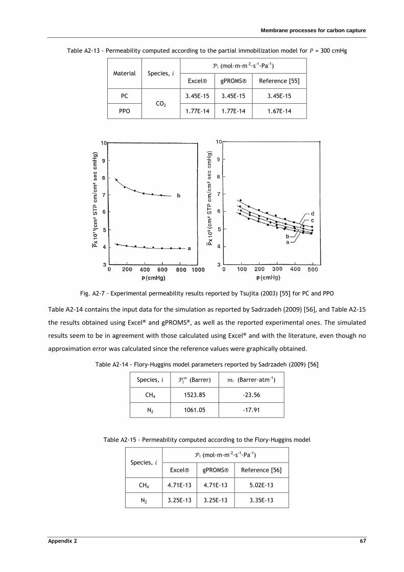
Membrane processes for carbon capture
Appendix 2 67
Table A2-13 - Permeability computed according to the partial immobilization model for = 300 cmHg
Material Species, (mol∙m∙m-2∙s-1∙Pa-1)
Excel® gPROMS® Reference [55]
PC
CO2
3.45E-15 3.45E-15 3.45E-15
PPO 1.77E-14 1.77E-14 1.67E-14
Fig. A2-7 - Experimental permeability results reported by Tsujita (2003) [55] for PC and PPO
Table A2-14 contains the input data for the simulation as reported by Sadrzadeh (2009) [56], and Table A2-15
the results obtained using Excel® and gPROMS®, as well as the reported experimental ones. The simulated
results seem to be in agreement with those calculated using Excel® and with the literature, even though no
approximation error was calculated since the reference values were graphically obtained.
Table A2-14 - Flory-Huggins model parameters reported by Sadrzadeh (2009) [56]
Species, (Barrer) (Barrer∙atm-1)
CH4 1523.85 -23.56
N2 1061.05 -17.91
Table A2-15 - Permeability computed according to the Flory-Huggins model
Species, (mol∙m∙m-2∙s-1∙Pa-1)
Excel® gPROMS® Reference [56]
CH4 4.71E-13 4.71E-13 5.02E-13
N2 3.25E-13 3.25E-13 3.35E-13

Membrane processes for carbon capture
Appendix 2 68
Table A2-16 contains the input data for the simulation as reported by Lira and Paterson (2002) [38], and
Table A2-17 the results obtained for a pressure gradient of 0.6 bar using Excel® and gPROMS®, as well as the
reported experimental ones, which are illustrated in Fig. A2-8.
Table A2-16 - Pore-flow parameters reported by Lira and Paterson (2002) [38]
(m) 6.40E-08
0.13
1
(m) 2.30E-05
Table A2-17 - Permeability computed according to the pore-flow model for = 0.6 bar
Species, (mol∙m∙m-2∙s-1∙Pa-1)
Excel® gPROMS® Reference [12]
CO2 4.46E-10 4.55E-10 3.26E-10
N2 5.60E-10 5.59E-10 5.37E-10
H2 2.04E-09 2.04E-09 1.38E-09
Fig. A2-8 - Experimental flux results reported by Lira and Paterson (2002) [38]

Membrane processes for carbon capture
Appendix 2 69
Table A2-18 contains the input data for the simulation as reported by Shin et al (2005) [57], and Table A2-19
the results obtained for a feed pressure of 200 kPa using Excel® and gPROMS®, as well as the reported
experimental ones, which are illustrated in Fig. A2-9.
Table A2-18 - Pore-flow parameters reported by Shin et al (2005) [57]
Sample S-A S-B S-C S-D
(m) 8.00E-08 8.00E-08 9.00E-08 1.05E-06
0.3500 0.3528 0.4795 0.4256
1 1 1 1
(m) 8.00E-04 1.00E-03 1.70E-03 1.70E-03
Table A2-19 - Permeability computed according to the pore-flow model for = 200 kPa
Species, Sample
(mol∙m∙m-2∙s-1∙Pa-1)
Excel® gPROMS® Reference [57]
N2
S-A 2.11E-09 2.11E-09 1.84E-09
S-B 2.12E-09 2.12E-09 1.90E-09
S-C 3.31E-09 3.31E-09 3.91E-09
S-D 7.04E-08 9.50E-08 5.10E-08
Fig. A2-9 - Experimental permeance results reported by Shin et al (2005) [57]
Table A2-20 contains the input data for the simulation as reported by Lito et al (2011) [59], and Table A2-21
the results obtained for a temperature of 338 K using Excel® and gPROMS®, as well as the reported
experimental ones, which are illustrated in Fig. A2-10.

Membrane processes for carbon capture
Appendix 2 70
Table A2-20 - Surface diffusion parameters reported by Lito et al (2011) [59] for a Langmuir isotherm
1 (m) Species, (mol∙kg-1) (Pa-1) (g∙m-3)
(m2∙s-1) (kJ∙mol-1)
0 3.50E-06 CO 3.37 2.40E-06 1.90E+06 1.88E-05 35.75
Table A2-21 - Permeability computed according to the surface diffusion model for = 338 kPa
Species, (mol∙m∙m-2∙s-1∙Pa-1)
Excel® gPROMS® Reference [59]
CO 6.82E-13 6.81E-13 7.00E-13
Fig. A2-10 - Experimental permeance results reported by Lito et al (2011) [59] for a Langmuir isotherm
Table A2-22 comprises the input data for the simulation as reported by Lagorsse et al (2004) [39], and Table
A2-23 the results obtained for a feed pressure of 2 bar at both temperatures using Excel® and gPROMS®, as
well as the reported experimental ones, which are illustrated in Fig. A2-11.
Table A2-22 - Surface diffusion parameters reported by Lagorsse et al (2004) [39] for a Langmuir isotherm
(m) Species, (K) (mol∙m-3) (bar-1) (m2∙s-1)
0.21 9.00E-06 N2
303 2719 0.19 4.20E-13
323 2147 0.15 8.60E-13
1 Porosity, , is null seeing that the zeolite density provided in the reference, , is apparent and therefore already
takes porosity into account

Membrane processes for carbon capture
Appendix 2 71
Table A2-23 - Permeability computed according to the surface diffusion model for = 2 bar
Species, (K)
(mol∙m∙m-2∙s-1∙Pa-1)
Excel® gPROMS® Reference [39]
N2
303 1.34E-15 1.33E-15 2.01E-15
323 1.79E-15 1.78E-15 2.81E-15
Fig. A2-11 - Experimental results reported by Lagorsse et al (2004) [39] for N2 at 303 (▲) and 323 K (▲)
Table A2-24 contains the individual mass transfer coefficients reported in by Dingemans et al (2008) [34], i,
from which the permeabilities in Table A2-25 were calculated to be used as input data for the simulation.
Table A2-26 contains the equivalent permeability results obtained using Excel® and gPROMS®, as well as the
reported experimental ones after processing.
Table A2-24 - Mass transfer coefficients reported by Dingemans et al (2008) [34]
Species, Material Layer (m) (m∙s-1)
TCE
PP/PVDF/PDMS
Dense 2.00E-06 7.17E-02
Porous 2.40E-04 2.64E-03
Polyester/PAN/PDMS
Dense 3.00E-07 4.78E-01
Porous 1.81E-04 4.32E-03

Membrane processes for carbon capture
Appendix 2 72
Table A2-25 - Layer resistance and permeability computed according to equation (3.2)
Species, Material Layer (s∙m-1) (m2∙s-1)
TCE
PP/PVDF/PDMS
Dense 1.39E+01 1.43E-07
Porous 3.79E+02 6.34E-07
Polyester /PAN/PDMS
Dense 2.09E+00 1.43E-07
Porous 2.31E+02 7.82E-07
Table A2-26 - Equivalent permeability computed according to the resistances in series model
Species, Material
(m2∙s-1)
Relative error (%)
Excel® gPROMS® Reference [34]
TCE
PP/PVDF/PDMS 6.16E-07 6.17E-07 5.74E-07 7.49
PET/PAN/PDMS 7.76E-07 7.76E-07 7.80E-07 0.43
Table A2-27 contains the input data for the simulation as reported by Dorosti et al (2011) [60], and Table A2-
28 comprises the results obtained for using Excel® and gPROMS®, as well as the reported experimental ones.
Table A2-27 - Resistances in parallel model parameters reported by Dorosti et al (2011) [60]
Species, (Barrer)
Continuous phase Disperse phase
CO2 1.7035 1.2502
N2 0.3650 0.2007
CH4 0.3795 0.2481

Membrane processes for carbon capture
Appendix 2 73
Table A2-28 - Equivalent permeability computed according to the resistances in parallel model
Species,
(mol∙m∙m-2∙s-1∙Pa-1)
Relative error (%)
Excel® gPROMS® Reference [60]
CO2
0.3 5.25E-16 5.25E-16 5.46E-16 3.84
0.5 4.95E-16 4.95E-16 4.56E-16 8.40
0.7 4.64E-16 4.64E-16 4.66E-16 0.33
N2
0.3 1.06E-16 1.06E-16 1.07E-16 1.53
0.5 9.47E-17 9.47E-17 9.08E-17 4.30
0.7 8.37E-17 8.37E-17 9.75E-17 14.15
CH4
0.3 1.14E-16 1.14E-16 1.21E-16 5.82
0.5 1.05E-16 1.05E-16 9.49E-17 10.76
0.7 9.63E-17 9.63E-17 9.75E-17 1.27
Table A2-29 contains the input data for the simulation as reported by Gheimasi et al (2014) [36], and Table
A2-30 the results obtained for using Excel® and gPROMS®, as well as the reported experimental ones.
Table A2-29 - Maxwell model parameters reported by Gheimasi et al (2014) [36]
Species, (cm3(STP)∙cm∙cm-2∙s-1∙mm Hg-1)
Continuous phase Disperse phase
CO2 4.45E-11 9.56E-09
Table A2-30 - Equivalent permeability computed according to the Maxwell model
Species,
(mol∙m∙m-2∙s-1∙Pa-1)
Relative error (%)
Excel® gPROMS® Reference [36]
CO2
0.02 1.58E-15 1.58E-15 1.52E-15 4.17
0.05 1.72E-15 1.72E-15 1.60E-15 7.63
0.10 1.98E-15 1.98E-15 1.67E-15 18.45
0.15 2.27E-15 2.27E-15 1.81E-15 25.10
0.20 2.59E-15 2.59E-15 2.00E-15 29.70

Membrane processes for carbon capture
Appendix 3 74
Appendix 3 gPROMS® flowsheeting
A3.1 Simulation and validation
Table A3-1 comprises the sensitivity analysis performed in order to assess the equivalence of simulating
single- and multiple-module stages with the same total permeation area while Table A3-2 features the size
specifications of the membrane modules allegedly employed in the installation reported by Choi et al (2013)
and used in cases 1 through 3C, which in turn are listed in Table A3-3.
Table A3-1 - First stage recovery for cases 1 through 3A using single and multiple membrane modules
Case Single module Multiple module
1 0.758954 0.761246
2 0.784544 0.798394
3A 0.787439 0.797913
Table A3-2 - Size specifications of the membrane modules allegedly employed in the installation reported by Choi
et al (2013) [46]
(cm) 50 16,000
(μm) 4 (cm2) 7.6
(μm) 2 (mm) 76
Table A3-3 - Case conditions reported by Choi et al (2013) [46]
Case Stage Number of
modules (exp.)
Number of
modules (sim.)
(bar) (bar)
(mol∙m-2∙s-1∙Pa-1)
(mol∙m-2∙s-1∙Pa-1)
1
1 20 15 5.884 0.981 1.506E-08 7.750E-10
2 3 2 5.884 0.981 1.535E-08 9.088E-10
3 1 1 5.884 0.981 1.593E-08 1.340E-09
4 1 1 2.940 0.981 1.560E-08 1.059E-09
2
1 10 9 5.884 0.196 1.506E-08 7.750E-10
2 3 2 5.884 0.981 1.560E-08 1.057E-09
3 1 1 5.884 0.981 1.612E-08 1.578E-09
4 1 1 2.940 0.981 1.562E-08 1.074E-09

Membrane processes for carbon capture
Appendix 3 75
Table A3-3 (cont.) - Case conditions reported by Choi et al (2013) [46]
Case Stage Number of
modules (exp.)
Number of
modules (sim.)
(bar) (bar)
(mol∙m-2∙s-1∙Pa-1)
(mol∙m-2∙s-1∙Pa-1)
3A
1 10 9 5.884 0.196 1.507E-08 7.783E-10
2 3 2 5.884 0.196 1.560E-08 1.060E-09
3 1 1 5.884 0.981 1.619E-08 1.685E-09
4 1 1 2.940 0.981 1.568E-08 1.117E-09
3B
1 10 9 6.628 0.173 1.508E-08 7.842E-10
2 3 2 6.628 0.163 1.569E-08 1.123E-09
3 1 1 4.079 1.020 1.577E-08 1.193E-09
4 1 1 3.263 1.020 1.576E-08 1.182E-09
3C
1 10 9 7.138 0.173 1.510E-08 7.906E-10
2 3 2 6.628 0.224 1.569E-08 1.123E-09
3 1 1 4.589 1.020 1.585E-08 1.259E-09
4 1 1 3.365 1.020 1.573E-08 1.155E-09
Fig. A3-1 depicts the linear fits to experimental permeation data reported by Choi et al (2013) while Fig. A3-2
illustrates the gPROMS® topology used to simulate the flowsheet reported in the same reference, and Table
A3-4 and Table A3-5 comprise the size specifications of the single-module membrane stages simulated for
cases 1 through 3C.
Fig. A3-1 - Linear fits to data reported by Choi et al (2013) [46] for permeance and selectivity
y = 3E-10x + 1E-08 R² = = 0.999
y = -2,467x + 21 R² = 1
0
5
10
15
20
25
0,0E+00
2,0E-09
4,0E-09
6,0E-09
8,0E-09
1,0E-08
1,2E-08
1,4E-08
1,6E-08
1,8E-08
0 2 4 6
Se
lectiv
ity P
erm
ea
nce
(m
ol∙m
-2∙s
-1∙Pa
-1)
CO2 feed partial pressure (bar)
Permeance CO2
Permeance N2
Selectivity CO2/N2
Linear (Permeance CO2)
Linear (Selectivity CO2/N2)

Membrane processes for carbon capture
Appendix 3 76
Fig. A3-2 - gPROMS® topology relative to the flowsheet reported by Choi et al (2013) [46]
Table A3-4 - Membrane module size specifications used for case 1
Stage 1 2 3 4
(m) 1 1.5 0.5 0.5
160,000 16,000 16,000 16,000
(m2) 150.8 22.6 7.6 7.6
(m) 0.239 0.076 0.076 0.076
Table A3-5 - Membrane module size specifications used for cases 2, 3A, 3B and 3C
Stage 1 2 3 4
(m) 1 1.5 0.5 0.5
72,000 16,000 16,000 16,000
(m2) 75.4 22.6 7.6 7.6
(m) 0.169 0.076 0.076 0.076
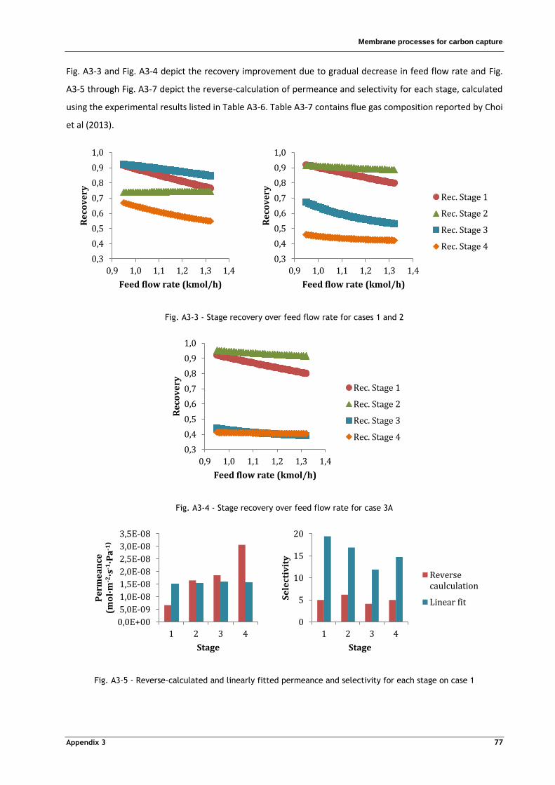
Membrane processes for carbon capture
Appendix 3 77
Fig. A3-3 and Fig. A3-4 depict the recovery improvement due to gradual decrease in feed flow rate and Fig.
A3-5 through Fig. A3-7 depict the reverse-calculation of permeance and selectivity for each stage, calculated
using the experimental results listed in Table A3-6. Table A3-7 contains flue gas composition reported by Choi
et al (2013).
Fig. A3-3 - Stage recovery over feed flow rate for cases 1 and 2
Fig. A3-4 - Stage recovery over feed flow rate for case 3A
Fig. A3-5 - Reverse-calculated and linearly fitted permeance and selectivity for each stage on case 1
0,3
0,4
0,5
0,6
0,7
0,8
0,9
1,0
0,9 1,0 1,1 1,2 1,3 1,4
Re
cov
ery
Feed flow rate (kmol/h)
0,3
0,4
0,5
0,6
0,7
0,8
0,9
1,0
0,9 1,0 1,1 1,2 1,3 1,4 R
eco
ve
ry
Feed flow rate (kmol/h)
Rec. Stage 1
Rec. Stage 2
Rec. Stage 3
Rec. Stage 4
0,3
0,4
0,5
0,6
0,7
0,8
0,9
1,0
0,9 1,0 1,1 1,2 1,3 1,4
Re
cov
ery
Feed flow rate (kmol/h)
Rec. Stage 1
Rec. Stage 2
Rec. Stage 3
Rec. Stage 4
0,0E+00
5,0E-09
1,0E-08
1,5E-08
2,0E-08
2,5E-08
3,0E-08
3,5E-08
1 2 3 4
Pe
rme
an
ce
(m
ol∙m
-2∙s
-1∙Pa
-1)
Stage
0
5
10
15
20
1 2 3 4
Se
lect
ivit
y
Stage
Reverse caulculation
Linear fit
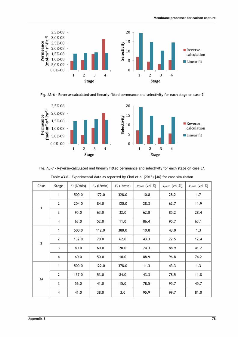
Membrane processes for carbon capture
Appendix 3 78
Fig. A3-6 - Reverse-calculated and linearly fitted permeance and selectivity for each stage on case 2
Fig. A3-7 - Reverse-calculated and linearly fitted permeance and selectivity for each stage on case 3A
Table A3-6 - Experimental data as reported by Choi et al (2013) [46] for case simulation
Case Stage (l/min) (l/min) (l/min) (vol.%) (vol.%) (vol.%)
1
1 500.0 172.0 328.0 10.8 28.2 1.7
2 204.0 84.0 120.0 28.3 62.7 11.9
3 95.0 63.0 32.0 62.8 85.2 28.4
4 63.0 52.0 11.0 86.4 95.7 63.1
2
1 500.0 112.0 388.0 10.8 43.0 1.3
2 132.0 70.0 62.0 43.3 72.5 12.4
3 80.0 60.0 20.0 74.3 88.9 41.2
4 60.0 50.0 10.0 88.9 96.8 74.2
3A
1 500.0 122.0 378.0 11.3 43.3 1.3
2 137.0 53.0 84.0 43.3 78.5 11.8
3 56.0 41.0 15.0 78.5 95.7 45.7
4 41.0 38.0 3.0 95.9 99.7 81.0
0,0E+00
5,0E-09
1,0E-08
1,5E-08
2,0E-08
2,5E-08
3,0E-08
3,5E-08
1 2 3 4
Pe
rme
an
ce
(m
ol∙m
-2∙s
-1∙Pa
-1)
Stage
0
5
10
15
20
1 2 3 4
Se
lect
ivit
y
Stage
Reverse calculation
Linear fit
0,0E+00
5,0E-09
1,0E-08
1,5E-08
2,0E-08
2,5E-08
1 2 3 4
Pe
rme
an
ce
(m
ol∙m
-2∙s
-1∙Pa
-1)
Stage
0
5
10
15
20
1 2 3 4
Se
lect
ivit
y
Stage
Reverse calculation
Linear fit

Membrane processes for carbon capture
Appendix 3 79
Table A3-6 (cont.) - Experimental data as reported by Choi et al (2013) [46] for case simulation
Case Stage (l/min) (l/min) (l/min) (vol.%) (vol.%) (vol.%)
3B
1 500 137 --/-- 10.8 43.0 --/--
2 128 74 --/-- 43.0 77.3 --/--
3 61 52 --/-- 77.3 95.2 --/--
4 46 49 --/-- 95.2 98.2 --/--
3C
1 500 137 --/-- 10.8 37.2 --/--
2 162 74 --/-- 37.2 75.6 --/--
3 77 52 --/-- 75.6 94.3 --/--
4 52 49 --/-- 94.3 97.0 --/--
Table A3-7 - Flue gas composition reported by Choi et al (2013) [46]
Component Volume fraction (vol.%)
N2 87.2
O2 2.0
CO2 10.8
A3.2 Optimisation and sensitivity analysis
Fig. A3-8 depicts the linear fits to the performance data reported by Liu et al (2014) [47] for HF
Matrimid®/PDMS composite module, from which the free volume parameters in table
Table A3-8 were determined.
Fig. A3-8 - Linear fit to permeability data reported by Liu et al (2014) [47]
y = -892.12x - 21.772 R² = 0.986
y = -2474.3x - 19.908 R² = 0.998
-32
-30
-28
-26
-24
-22
-20
3,0E-03 3,5E-03 4,0E-03 4,5E-03
ln(
) (m
ol∙m∙m
-2∙s
-1∙Pa
-1)
1/T (K-1)
Permeability N2
Permeability CO2
Linear (Permeability N2)
Linear (Permeability CO2)
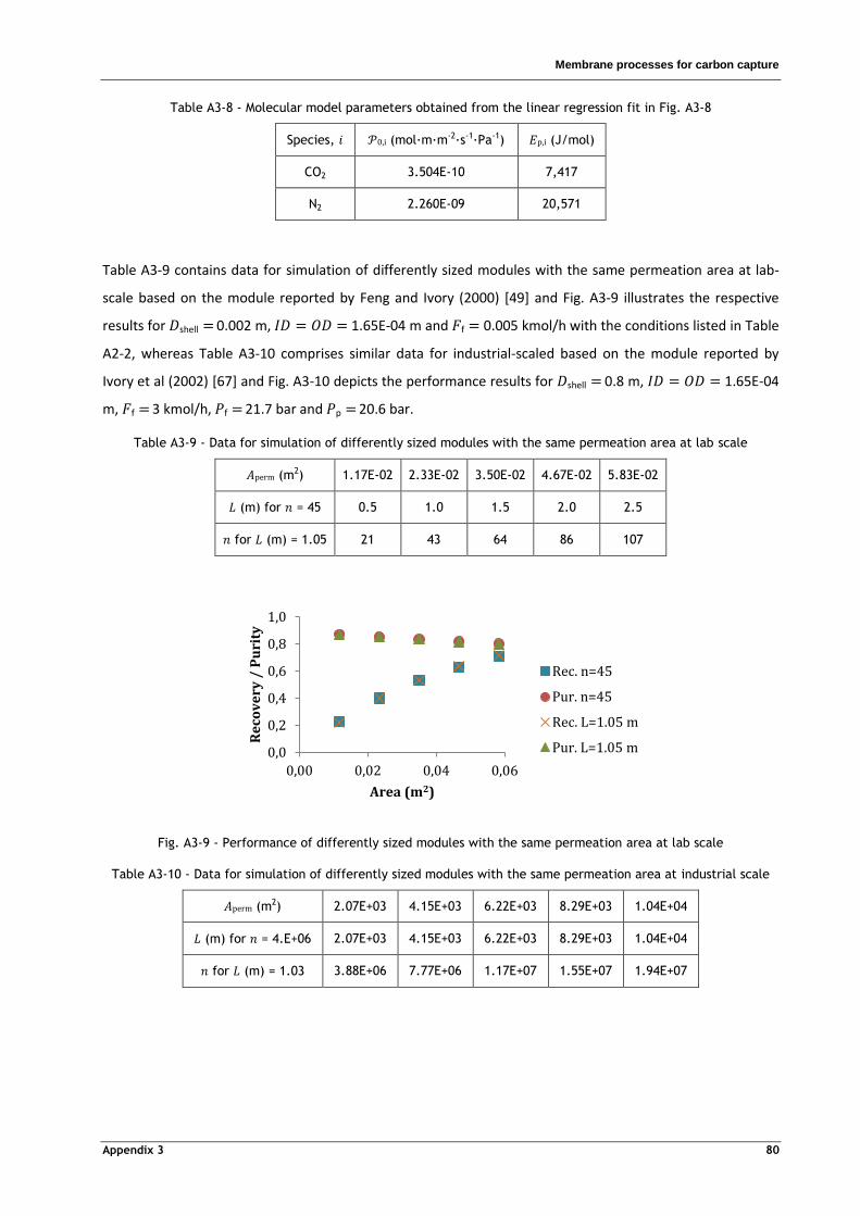
Membrane processes for carbon capture
Appendix 3 80
Table A3-8 - Molecular model parameters obtained from the linear regression fit in Fig. A3-8
Species, (mol∙m∙m-2∙s-1∙Pa-1) (J/mol)
CO2 3.504E-10 7,417
N2 2.260E-09 20,571
Table A3-9 contains data for simulation of differently sized modules with the same permeation area at lab-
scale based on the module reported by Feng and Ivory (2000) [49] and Fig. A3-9 illustrates the respective
results for shell 0.002 m, 1.65E-04 m and f 0.005 kmol/h with the conditions listed in Table
A2-2, whereas Table A3-10 comprises similar data for industrial-scaled based on the module reported by
Ivory et al (2002) [67] and Fig. A3-10 depicts the performance results for shell 0.8 m, 1.65E-04
m, f 3 kmol/h, f 21.7 bar and p 20.6 bar.
Table A3-9 - Data for simulation of differently sized modules with the same permeation area at lab scale
(m2) 1.17E-02 2.33E-02 3.50E-02 4.67E-02 5.83E-02
(m) for = 45 0.5 1.0 1.5 2.0 2.5
for (m) = 1.05 21 43 64 86 107
Fig. A3-9 - Performance of differently sized modules with the same permeation area at lab scale
Table A3-10 - Data for simulation of differently sized modules with the same permeation area at industrial scale
(m2) 2.07E+03 4.15E+03 6.22E+03 8.29E+03 1.04E+04
(m) for = 4.E+06 2.07E+03 4.15E+03 6.22E+03 8.29E+03 1.04E+04
for (m) = 1.03 3.88E+06 7.77E+06 1.17E+07 1.55E+07 1.94E+07
0,0
0,2
0,4
0,6
0,8
1,0
0,00 0,02 0,04 0,06
Re
cov
ery
/ P
uri
ty
Area (m2)
Rec. n=45
Pur. n=45
Rec. L=1.05 m
Pur. L=1.05 m
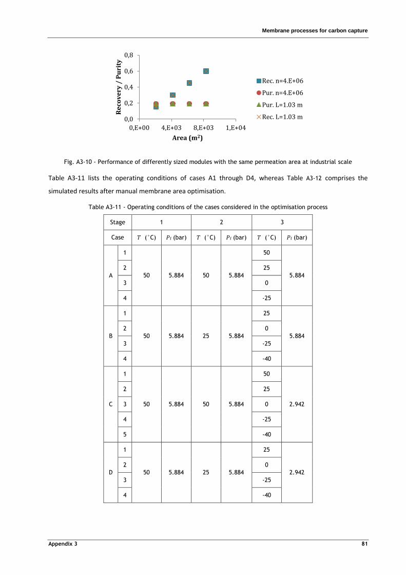
Membrane processes for carbon capture
Appendix 3 81
Fig. A3-10 - Performance of differently sized modules with the same permeation area at industrial scale
Table A3-11 lists the operating conditions of cases A1 through D4, whereas Table A3-12 comprises the
simulated results after manual membrane area optimisation.
Table A3-11 - Operating conditions of the cases considered in the optimisation process
Stage 1 2 3
Case (°C) (bar) (°C) (bar) (°C) (bar)
A
1
50 5.884 50 5.884
50
5.884
2 25
3 0
4 -25
B
1
50 5.884 25 5.884
25
5.884
2 0
3 -25
4 -40
C
1
50 5.884 50 5.884
50
2.942
2 25
3 0
4 -25
5 -40
D
1
50 5.884 25 5.884
25
2.942
2 0
3 -25
4 -40
0,0
0,2
0,4
0,6
0,8
0,E+00 4,E+03 8,E+03 1,E+04
Re
cov
ery
/ P
uri
ty
Area (m2)
Rec. n=4.E+06
Pur. n=4.E+06
Pur. L=1.03 m
Rec. L=1.03 m
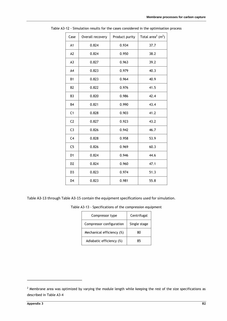
Membrane processes for carbon capture
Appendix 3 82
Table A3-12 - Simulation results for the cases considered in the optimisation process
Case Overall recovery Product purity Total area2 (m2)
A1 0.824 0.934 37.7
A2 0.824 0.950 38.2
A3 0.827 0.963 39.2
A4 0.823 0.979 40.3
B1 0.823 0.964 40.9
B2 0.822 0.976 41.5
B3 0.820 0.986 42.4
B4 0.821 0.990 43.4
C1 0.828 0.903 41.2
C2 0.827 0.923 43.2
C3 0.826 0.942 46.7
C4 0.828 0.958 53.9
C5 0.826 0.969 60.3
D1 0.824 0.946 44.6
D2 0.824 0.960 47.1
D3 0.823 0.974 51.3
D4 0.823 0.981 55.8
Table A3-13 through Table A3-15 contain the equipment specifications used for simulation.
Table A3-13 - Specifications of the compression equipment
Compressor type Centrifugal
Compressor configuration Single stage
Mechanical efficiency (%) 80
Adiabatic efficiency (%) 85
2 Membrane area was optimized by varying the module length while keeping the rest of the size specifications as
described in Table A3-4

Membrane processes for carbon capture
Appendix 3 83
Table A3-14 - Specifications of the vacuum equipment
Pump type Vacuum
Mechanical efficiency (%) 80
Ideal efficiency (%) 75
Table A3-15 - Specifications of the cooling equipment
Type of heat exchanger Shell-and-tube
Pressure drop (bar) 0
Heat exchanger area (m2) 1
A3.2 Industrial scale-up
Table A3-16 lists the membrane module size specifications used for the simulation of case D2 at industrial
scale.
Table A3-16 - Membrane module size specifications used for the simulation of scaled-up case D2
Stage 1 2 3
(m) 1.03 1.40 0.50
3.079E+09 8.097E+08 1.679E+09
(m2) 2.989E+06 1.068E+06 7.912E+05
(m) 33.2 19.7 24.5
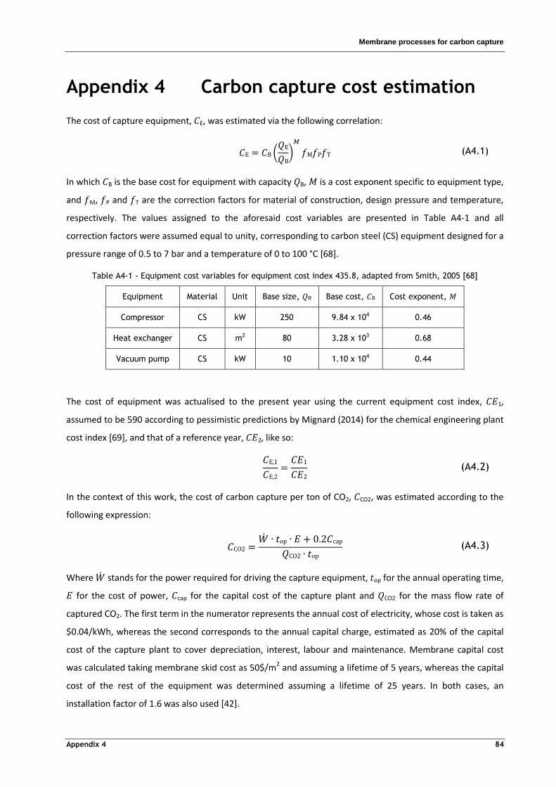
Membrane processes for carbon capture
Appendix 4 84
Appendix 4 Carbon capture cost estimation
The cost of capture equipment, , was estimated via the following correlation:
(A4.1)
In which is the base cost for equipment with capacity , is a cost exponent specific to equipment type,
and , P and are the correction factors for material of construction, design pressure and temperature,
respectively. The values assigned to the aforesaid cost variables are presented in Table A4-1 and all
correction factors were assumed equal to unity, corresponding to carbon steel (CS) equipment designed for a
pressure range of 0.5 to 7 bar and a temperature of 0 to 100 °C [68].
Table A4-1 - Equipment cost variables for equipment cost index 435.8, adapted from Smith, 2005 [68]
Equipment Material Unit Base size, Base cost, Cost exponent,
Compressor CS kW 250 9.84 x 10⁴ 0.46
Heat exchanger CS m2 80 3.28 x 10³ 0.68
Vacuum pump CS kW 10 1.10 x 10⁴ 0.44
The cost of equipment was actualised to the present year using the current equipment cost index, ,
assumed to be 590 according to pessimistic predictions by Mignard (2014) for the chemical engineering plant
cost index [69], and that of a reference year, , like so:
(A4.2)
In the context of this work, the cost of carbon capture per ton of CO2, CO , was estimated according to the
following expression:
(A4.3)
Where stands for the power required for driving the capture equipment, op for the annual operating time,
for the cost of power, cap for the capital cost of the capture plant and CO for the mass flow rate of
captured CO2. The first term in the numerator represents the annual cost of electricity, whose cost is taken as
$0.04/kWh, whereas the second corresponds to the annual capital charge, estimated as 20% of the capital
cost of the capture plant to cover depreciation, interest, labour and maintenance. Membrane capital cost
was calculated taking membrane skid cost as 50$/m2 and assuming a lifetime of 5 years, whereas the capital
cost of the rest of the equipment was determined assuming a lifetime of 25 years. In both cases, an
installation factor of 1.6 was also used [42].