1

Integrated Management of Power Aware Computing & Communication

TechnologiesReview Meeting

Nader Bagherzadeh, Pai H. Chou, Fadi Kurdahi, UC Irvine

Jean-Luc Gaudiot, USC,Nazeeh Aranki, Benny Toomarian, JPL

DARPA Contract F33615-00-1-1719

June 13, 2001

JPL -- Pasadena, CA

2

Agenda

Administrative Review of milestones, schedule

Technical presentation Progress

Applications (UAV/DAATR, Rover, Deep Impact, distributed sensors) Scheduling (system-level pipelining) Advanced microarchitecture power modeling (SMT) Architecture (mode selection with overhead) Integration (Copper, JPL, COTS data sheet)

Lessons learned Challenges, issues Next accomplishments

Questions & action items review.

3

Quad Chart

Innovations Component-based power-aware design

Exploit off-the-shelf components & protocols Best price/performance, reliable, cheap to replace

CAD tool for global power policy optimization Optimal partitioning, scheduling, configuration Manage entire system, including mechanical & thermal

Power-aware reconfigurable architectures Reusable platform for many missions Bus segmentation, voltage / frequency scaling

Impact

Enhanced mission success More task for the same power Dramatic reduction in mission completion time

Cost saving over a variety of missions Reusable platform & design techniques Fast turnaround time by configuration, not redesign

Confidence in complex design points Provably correct functional/power constraints Retargetable optimization to eliminate overdesign Power protocol for massive scale

Behavior

Architecture

high-levelsimulation

functionalpartitioning& scheduling

compositionoperators

high-levelcomponents

behavioralsystem model

busses, protocols systemarchitecture

mapping system integration& synthesis

staticconfiguration

dynamic powermanagement

parameterizablecomponents

2Q 00

Kickoff

2Q 01 2Q 02

Static & hybrid optimizations partitioning / allocation scheduling bus segmentation voltage scaling

COTS component library

FireWire and I2C bus models

Static composition authoring

Architecture definition

High-level simulation

Benchmark Identification

Dynamic optimizations task migration processor shutdown bus segmentation frequency scaling

Parameterizable components library

Generalized bus models

Dynamic reconfiguration authoring

Architecture reconfiguration

Low-level simulation

System benchmarking

Year 1 Year 2

4

Program Overview

Power-aware system-level design Amdahl's law applies to power as well as performance Enhance mission success (time, task) Rapid customization for different missions

Design tool Exploration & evaluation Optimization& specialization Technique integration

System architecture Statically configurable Dynamically adaptive Use COTS parts & protocols

5

Personnel & teaming plans

UC Irvine - Design tools Nader Bagherzadeh - PI Pai Chou - Co-PI Fadi Kurdahi Jinfeng Liu Dexin Li Duan Tran

USC - Component power optimization Jean-Luc Gaudiot - faculty participant Seong-Won Lee - student

JPL - Applications & benchmarking Nazeeh Aranki Nikzad “Benny” Toomarian

- students

6

Milestones & Schedule

Static & hybrid optimizationspartitioning / allocationschedulingbus segmentationvoltage scaling

COTS component library

FireWire and I2C bus models

Static composition authoring

Architecture definition

High-level simulation

Benchmark Identification

Dynamic optimizations task migrationprocessor shutdownbus segmentation frequency scaling

Parameterizable components library

Generalized bus models

Dynamic reconfiguration authoring

Architecture reconfiguration

Low-level simulation

System benchmarking

7

we are here!

Review of Progress

May'00 Kickoff meeting (Scottsdale, AZ)

Sept'00 Review meeting (UCI) Scheduling formulation, UI mockup, System level configuration Examples: Pathfinder & X-2000 (manual solution)

Nov'00 PI meeting (Annapolis, MD) Tools: scheduler + UI v.1 (Java) Examples: Pathfinder & X-2000 (automated)

Apr'01 PI meeting (San Diego, CA) Tools: scheduler + UI v.2 - v.3 (Jython) Examples: Pathfinder & initial UAV (Pipelined)

June'01 Review meeting

8

New for this Review (June '01)

Tools Scheduler + UI v.4 (pipelined, buffer matching) Mode selector v.1 (mode change overhead, constraint based) SMT model

Examples: Pathfinder, µAMPS sensors (mode selection) UAV, Wavelet (dataflow) (pipelined, detailed estimate) Deep Impact (command driven) (planning)

Integration Input from Copper:

timing/power estimation (PowerPC simulation model) Output to Copper:

power profile + budget (Copper Compiler) Within IMPACCT:

initial Scheduler + Mode Selector integration

9

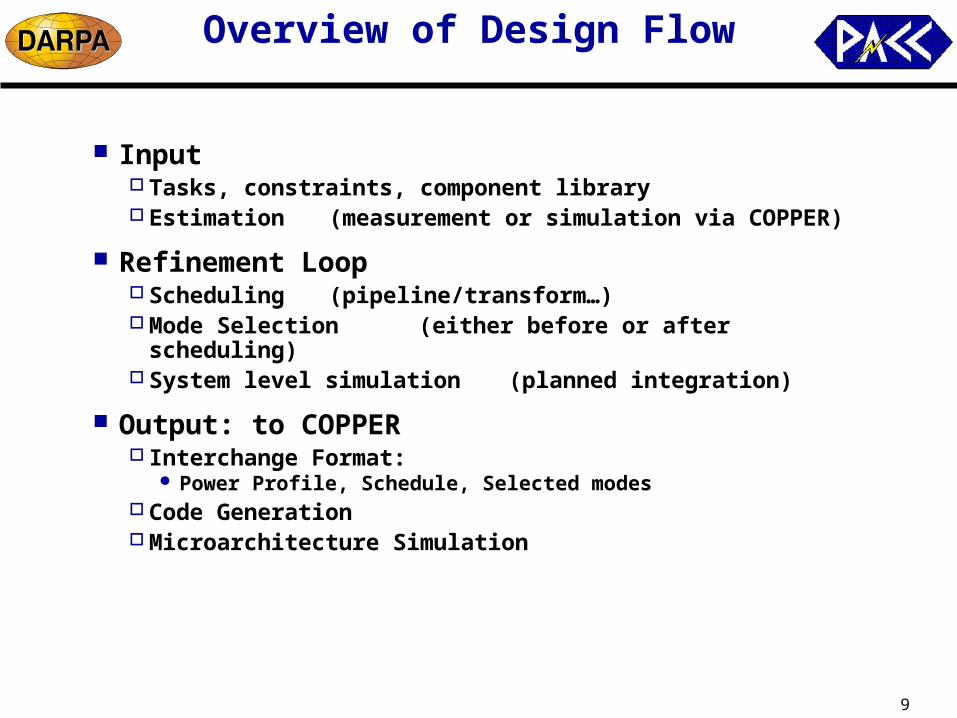
Overview of Design Flow

Input Tasks, constraints, component library Estimation (measurement or simulation via COPPER)

Refinement Loop Scheduling (pipeline/transform…) Mode Selection (either before or after scheduling) System level simulation (planned integration)

Output: to COPPER Interchange Format:

Power Profile, Schedule, Selected modes Code Generation Microarchitecture Simulation

10

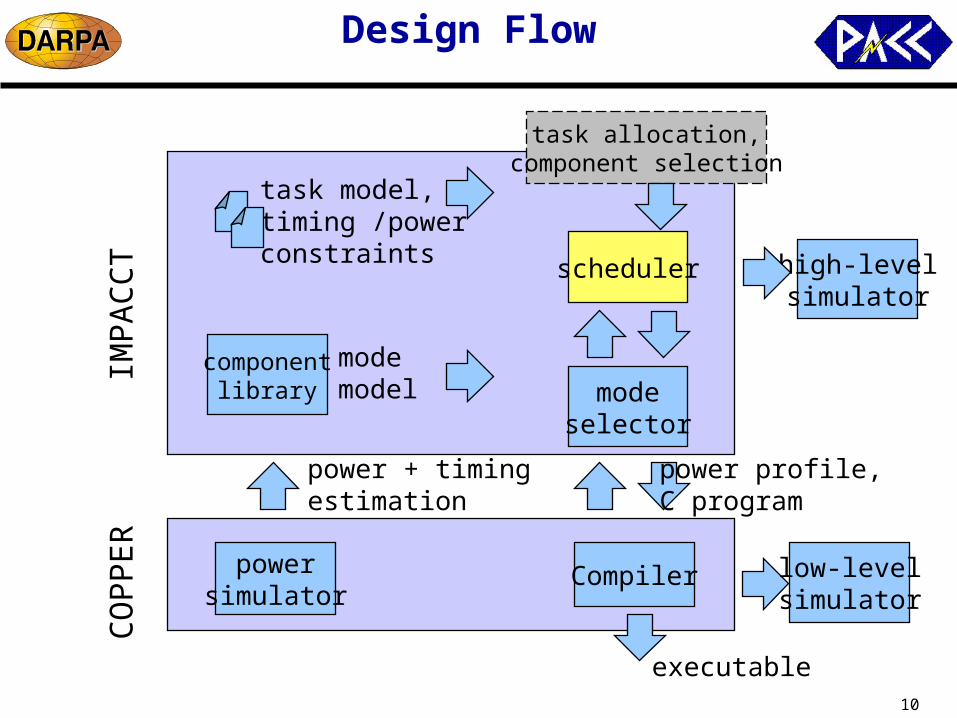
Design Flow

componentlibrary

scheduler high-levelsimulator

modeselector

powersimulator

task model,timing /powerconstraints

Compiler

power profile,C program

modemodel

power + timingestimation

task allocation,component selection

CO

PP

ER

IMP

AC

CT

low-levelsimulator

executable

11

Power Aware Scheduling

Execution model Multiple processors, multiple power consumers Multiple domains: digital, thermal, mechanical

Constraint driven Min / Max power Min / Max timing constraints

Handles problems in different domains Time Driven System level pipelining -- in time and in space Parallelism extraction

Experimental results Coarse to fine grained parallelism tradeoffs

12

Prototype of GUI scheduling tool

Power-aware Gantt chart Time view

Timing of all tasks on parallel resources

Power consumption of each task Power view

System-level power profile Min/max power constraint, energy

cost

Interactive scheduling Automated schedulers – timing,

power, loop Manual intervention – drag &

drop

Demo available

13

Power-Aware Scheduling

New constraint-based application model [paper at Codes'01] Min/Max Timing constraints

Precedence, subsumes dataflow, general timing, shared resource Dependency across iteration boundaries – loop pipelining Execution delay of tasks – enables frequency/voltage scaling

Power constraints Max power – total power budget Min power – controls power jitter or force utilization of free source

System-level, multi-scenario scheduling [paper at DAC'01] 25% Faster while saving 31% energy cost Exploits "free" power (solar, nuclear min-output)

System-level loop pipelining [working papers] Borrow time and power across iteration boundaries Aggressive design space exploration by new constraint classification Achieves 49% speedup and 24% energy reduction

14

Scheduling case study:Mars Pathfinder

System specification 6 wheel motors 4 steering motors System health check Hazard detection

Power supply Battery (non-rechargeable) Solar panel

Power consumption Digital

Computation, imaging, communication, control Mechanical

Driving, steering Thermal

Motors must be heated in low-temperature environment

15

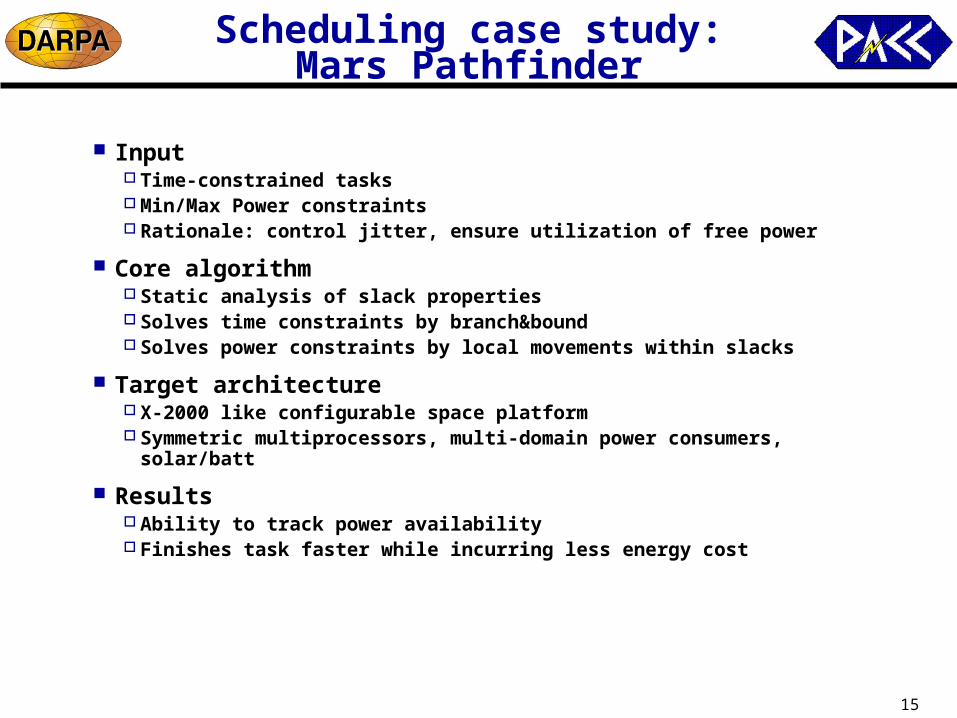
Scheduling case study:Mars Pathfinder

Input Time-constrained tasks Min/Max Power constraints Rationale: control jitter, ensure utilization of free power

Core algorithm Static analysis of slack properties Solves time constraints by branch&bound Solves power constraints by local movements within slacks

Target architecture X-2000 like configurable space platform Symmetric multiprocessors, multi-domain power consumers, solar/batt

Results Ability to track power availability Finishes task faster while incurring less energy cost

16

More aggressive scheduling:System-level pipelining

Borrow tasks across iterations Alleviates "hot spots" by spreading to another iteration Smooth out utilization by borrowing across iterations

Core techniques Formulation: separate pseudo dependency from true dependency Static analysis and task transformation Augmented scheduler for new dependency

Results -- on Mars Pathfinder example Additional energy savings with speedup Smoother power profile

17

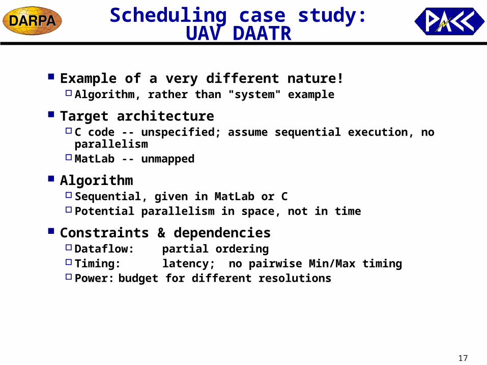
Scheduling case study:UAV DAATR

Example of a very different nature! Algorithm, rather than "system" example

Target architecture C code -- unspecified; assume sequential execution, no parallelism MatLab -- unmapped

Algorithm Sequential, given in MatLab or C Potential parallelism in space, not in time

Constraints & dependencies Dataflow: partial ordering Timing: latency; no pairwise Min/Max timing Power: budget for different resolutions

18

Scheduling case study:UAV example (cont'd)

Challenge: Parallelism Extraction Essential to enable scheduling Difficult to automate; need manual code rewrite Different pipeline stages must be relatively similar in length

Rewritten code Inserted checkpoints for power estimation Error prone buffer mapping between iterations

Found a dozen bugs in benchmark C code Missing Summation in standard deviation calculation Frame buffer off by one line Dangling pointers not exposed until pipelined

19

ATR application: what we are given

Target Detection

FFT

Filter/IFFT

Filter/IFFT

Filter/IFFT

ComputeDistance

ComputeDistance

1 Frame

m Detections3 filters

FFT FFT FFT

Filter/IFFT

Filter/IFFT

Filter/IFFT

ComputeDistance

ComputeDistance

FFT FFT

Bugs

20

Bug report

Misread input data file OK, no effect to the algorithm

Miscalculate mean, std for image OK, these values not used (currently)

Wrong filter data for SUN/PowerPC OK for us, since we operate on different platforms Bad for SUN/PowerPC users, wrong results

Misplaced FFT module The algorithm is wrong

If images are turned upside-down, the results are different Not sure whether it is correct

However, these problems are not captured in the output image files

21

What it should look like

Target Detection

FFT FFT

Filter/IFFT

Filter/IFFT

Filter/IFFT

ComputeDistance

ComputeDistance

ComputeDistance

ComputeDistance

Filter/IFFT

Filter/IFFT

Filter/IFFT

1 Frame

m Detections

3 filters

k distances

22

What it really should look like

Target Detection

FFT FFT

Filter/IFFT

Filter/IFFT

Filter/IFFT

ComputeDistance

ComputeDistance

ComputeDistance

ComputeDistance

Filter/IFFT

Filter/IFFT

Filter/IFFT

1 Frame

m Detections

3 filters

k distances

23

Problems

Limited parallelism Serial data flow with tight dependency Parallelism available (diff. detections, filters, etc) but limited

Limited ability to extract parallelism Limited by serial execution model (C implementation) No available parallel platforms

Limited scalability Cannot guarantee response time for big images (N2 complexity) Cannot apply optimization for small images (each block is too small)

Limited system-level knowledge High-level knowledge lost in a particular implementation

24

Our vision: 2-dimensional partitioning

M Targets(M FFTs)

M Targets(3M IFFTs)

K Distances(2K IFFTs)

Output: target detection w/ distance for N simultaneous frames

Target Detection

FFT

Filter/IFFT

ComputeDistance

m Detections

3 filters

k distances

Filter/IFFT

Filter/IFFT

ComputeDistance

FFT

Filter/IFFT

ComputeDistance

Filter/IFFT

Filter/IFFT

ComputeDistance

Single DFG(vertical flow)

Target Detection

FFT

Filter/IFFT

ComputeDistance

m Detections

3 filters

k distances

Filter/IFFT

Filter/IFFT

ComputeDistance

FFT

Filter/IFFT

ComputeDistance

Filter/IFFT

Filter/IFFT

ComputeDistance

Input:N simultaneous

frames

Cluster by N DFGs(horizontal duplication)

N Frames(N target detection)

Partitioning(horizontal cuts)

25

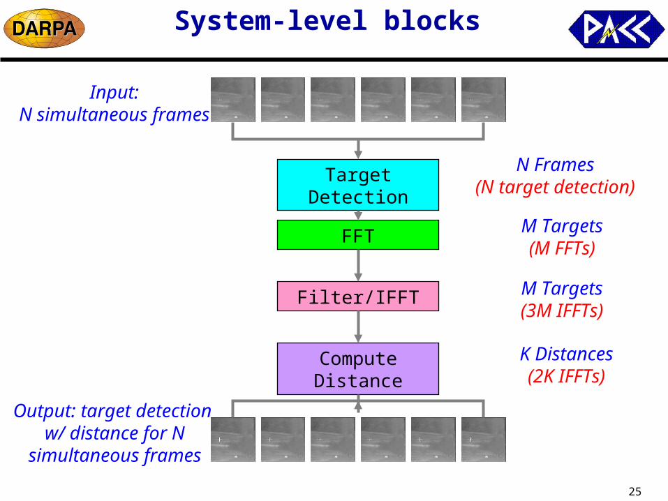
System-level blocks

Target Detection

FFT

Filter/IFFT

Compute Distance

N Frames(N target detection)

M Targets(M FFTs)

M Targets(3M IFFTs)

K Distances(2K IFFTs)

Input:N simultaneous frames

Output: target detection w/ distance for N

simultaneous frames

26

System-level pipelining

Target Detection

FFT

Filter/IFFT

Compute Distance

Input:N simultaneous frames

Output: target detection w/ distance for N

simultaneous frames

Group 0Group 1

Group 0

Group 2

Group 0

Group 1

Group 3

Group 0

Group 1

Group 2

Group 4

Group 3

Group 2

Group 1

Group 0

Group 5

Group 4

Group 3

Group 2

Group 1

27

What does it buy us?

Parallelism All modules run in PARALLEL Each module processes N (M, K) INDEPENDENT instances, that could

all be processed in parallel NO DATA DEPENDENCY between modules

Throughput Throughput multiplied by processing units Process N frames at a reduced response time Better utilization of resources

28

What does it buy us? (cont'd)

Flexibility Insert / remove modules at any time Adjust N, (M or K) at any time Make each module parallel / serial at any time More knobs to tune: parallelism / response time / throughput / power Driven by run-time constraints

Scalability Reduced response time on big images (small N and/or deeper pipe) Better utilization/throughput on small images

More compiler support Simple control / data flow: each module is just a simple loop, which is

essentially parallel Need an automatic partitioning tool to take horizontal cuts

29

What does it buy us: how power-aware is it?

Subsystems shut-down Turn on / off any time based on power budget Split / merge (migrate) modules on demand

Power-aware scheduling Each task can be scheduled at any time during one pipe stage, since

they are totally independent More scheduling opportunity with an entire system

Dynamic voltage/frequency scaling The amount of computation N, (M or K) is known ahead of time Scaling factor = C / N (very simple!) Less variance of code behavior =>

strong guarantee to meet deadline, more accurate power estimates

Run-time code versioning Select right code based on N, (M or K)

30

Experimental implementation:pipelining transformation

Goal To make everything completely independent

Methodology Dataflow graph extraction (vertical) Initial partitioning (currently manual with some aids from COPPER) Horizontal clustering Horizontal cut (final partitioning)

Techniques Buffer assignment: each module gets its own buffer Buffer renaming: read/write on different buffer Circular buffer: each module gets a window of fixed buffer size Our approach: the combination

31

Buffer rotation

B

Circular buffer B

Pipe stages:a, b, c, d

a

b

cd

Time = 0

a b c

dTime = 1

ab c

d

Time = 2

ab

c d

Time = 3a

bc

d

Time = 4a

bc

d

Time = 5

32

Background - acyclic dataflow

a

b

c

d

Single circular buffer One serial data flow path All data flows are of same type

same size

Multiple buffers Multiple data flow paths Different type, size

a

b

c

d

33

A more complete picture

ab c

d

Circular buffer A, B rotate at the same speed

Pipe stages:a, b, c, d

B

A

Time = 0Time = 1

B

A

B

A

Time = 2B

A

Time = 3Time = 4

B

A

Time = 5

B

A

2. Buffer live

3. Life-time spent in pipeline 4. Buffer dead

1. Buffer ready(raw data, e.g. ATR images)

Head pointer

34

How does it work?

Raw data is dumped into the buffer from the data sources A head pointer keeps incrementing Buffer is ready, but not live (active in pipeline) yet Example, ATR image data coming from sensors

Buffer becomes live in pipeline Raw data are consumed and/or forwarded New data are produced/consumed When a buffer is no longer needed by any pipeline stages, it is dead and

recycled

Is everything really independent? Yes! At each snapshot, each module is operating on different data

35

What are we trading off?

ab c

d

B

A

Speedcomputation intensity, parallelism,throughput,power

TimeResponse time,

delay

Workloadamount of computation, energy

a

bc

d

a b c dab c

da

b

cd

ab c d

36

N = 2

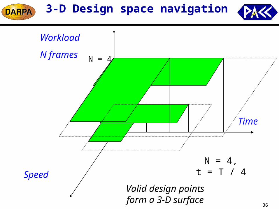
3-D Design space navigation

Speed

Time

Workload

N frames

N = 2,t = T / 2

N = 4,t = T / 4

N = 4

Valid design points form a 3-D surface

37

Design flow

IMPACCT pipeline code transformation

C Source code

Pipelined C Source code

COPPER power simulator

P T N

3-D table•Power•Time•Workload Task-level

constraints

System-level constraints

Power-aware schedule

IMPACCT scheduler and mode selection

abcd

DFG

38

Demo: power-aware ATR

Input N frames

Output N frames

Power-aware schedule and run-time power profile

Control panel, timing/power constraints, group size N

39

What it can do

Interactive performance monitor Run ATR (or any other) algorithms on PC, network or external boards Monitor power/performance at run-time Giving timing/power budget on the fly

System-level simulator Run ATR algorithms on (distributed) component-level simulators (e.g.

COPPER) Coordinate component-level simulators to construct the whole system Examine the power/performance on the system level with verified

results on components

40

What it can do

Dynamic power manager Apply dynamic power management policies Power management decision based on verified results from simulation Pre-examine different dynamic power management policies without the

real execution platform Out first stage to go dynamic

What’s in the current demo? ATR toolbox

Run ATR on different images Operate on all image formats, not only the .bin binary format

Performance monitor / simulator User inputs power/time/group size Power/time based on COPPER simulation results

Dynamic power manager Dynamic voltage/frequency scaling based on given timing constraints Only minimize power, not taking power budget into constraint yet

41

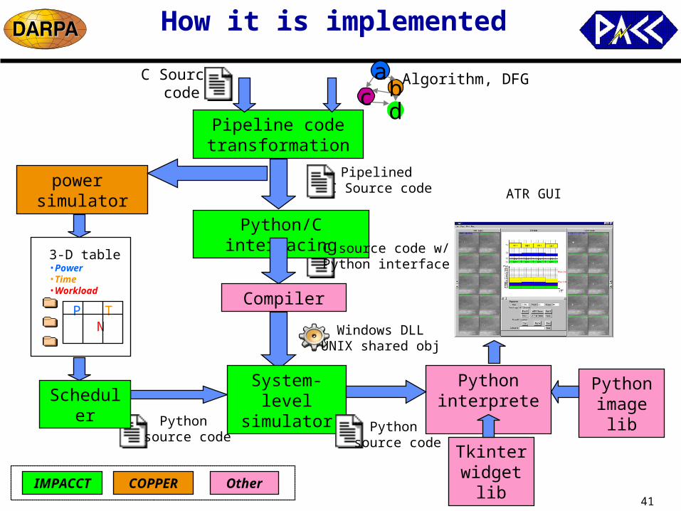
How it is implemented

Pipeline code transformation

C Source code

Pipelined C Source codepower

simulator

P T N

3-D table•Power•Time•Workload

abcd

Algorithm, DFG

Python/C interfacing

Scheduler

Compiler

C source code w/Python interface

Windows DLLUNIX shared obj

Python source code

System-level simulator

Pythoninterpreter

Python source code

Tkinterwidget lib

Pythonimage lib

ATR GUI

IMPACCT COPPER Other

42

What did we learn from this?

Component-level vs. system-level Component-level

Finer grain algorithms on specific data (FFT) Low-level programming (C code)

System-level Coerce grain algorithms on data flows (ATR) Increased level of programming (scripting, GUI)

System-level pipelining and code transformation More parallelism by eliminating data dependency Need automated compiler support

System-level simulation on ATR Can potentially plug in any other simulators, library modules Can integrate different component-level techniques Power management at system-level with more confidence Starting point to dynamic power management

43

Scheduling case study:Wavelet compression (JPL)

Algorithm in C Wavelet decomposition Compression: "knob" to choose lossy factor or lossless

Example category Dataflow, similar to DAATR Finer grained, better structure

IMPACCT improvements Transformation to enable pipelining Exploit lossy factor in trade space

44

Wavelet Algorithm

Wavelet Decomposition

Quantization

Entropy coding

45

Wavelet Algorithm structure

For all image blocks

Initialization(check params,

allocate memory)

block init.,set params, read image block

decomp(), (lossless FWT)

(remove overlap)

Bit_plane_decomp,(set decomp param)

(1st level entropy coding)

(bit_plane encoding) Output result to file

•Sequential execution blocks•No data dependency between image blocks

46

Wavelet: experiments

Experiments being conducted Checkpoints marked up manually Initial power estimation obtained Code being manually rewritten / restructured for pipelining Appears better structured than UAV example

Trade space High performance to low power Pipelining in space and in time, similar to UAV example Lossy compression parameter

47

Ongoing scheduling case study:Deep Impact

"Planning" level example Coarse grained, system level

Hardware architecture COTS PowerPC 750 babybed, emulating a Rad-Hard PPC at 4x

=> Models the X-2000 architecture using DS1 software COTS PowerPC 603e board, emulating I/O devices in real time

Software architecture vxWorks, static priority driven, preemptive JPL's own software architecture -- command based 1/8 second time steps; 1-second control loops

Task set 60 tasks to schedule, 255 priority levels

48

NASA Deep Impact project

Platform X-2000 configurable architecture to be using RAD 6000 (Rad-Hard PowerPC 750 @133MHz)

Testbed (JPL Autonomy Lab) PPC 750 single-board computer -- runs flight software

Prototype @233MHz, Real flight @133MHz COTS board, L1 only, no L2 cache

PowerPC 603e -- emulate the I/O devices connected via compact PCI

DS1: Deep Space One (legacy flight software ) Software architecture:

8 Hz ticks, command based running on top of vxWorks

Perfmon: performance monitoring utility in DS1 11 test activities 60 tasks

49

Deep Impact example (cont'd)

Available form: Real-time Traces Collected using Babybed 90 seconds of trace, time-stamped tasks, L-1 cache

Input needed Algorithm (not available) Timing / power constraints (easy) Functional constraints

Sequence of events Combinations of illegal modes

Challenges Modeling two layers of software architecture (RTOS + command)

50

Design Flow

componentlibrary

scheduler high-levelsimulator

modeselector

powersimulator

task model,timing /powerconstraints

Compiler

power profile,C program

modemodel

power + timingestimation

task allocation,component selection

CO

PP

ER

IMP

AC

CT

low-levelsimulator

executable

51

SMT Power Simulator

Simulator Features Compatible with SimpleScalar 3.0b

Execute PISA and EV6 binaries Portability – Run on most kinds of computers

Handling Simultaneous Multithreading Run up to 8 threads simultaneously Similar to UW SMT model

Power Aware Features Same analytic power model as WATTCH

Clock Gating Parameterized Models

42 functional unit classifications (WATTCH has 12) 10 dynamic activity factors (WATTCH has 4)

52

Examples of Module Classification

Functional Units include Arithmetic units: ALU, FPU, etc Control units: Instr decoder, etc Memory units: Caches, CAM, etc Buses: Result bus

Cache Access Cache Hit

Read Tag & Data Cache Miss

Read Tag Update Tag & Data Read Data

Arithmetic Operation: 4 groups Int ALU: +, -, bit operations Int MULT: , FP ALU: +, - FP MULT: ,

FP ALU

FP RegNormal FP Operation

FP MULT

FP RegFP Mult

Operation

ALU

Integer Reg

Integer ALU

Integer RegNormal Integer

Operation

Integer MULT

Integer RegInteger Mult Operation

Cache Tag X 2

Cache Array X 2Cache Miss

Cache Hit

Event

Cache

Cache Tag

Cache Array

Accessed units in WATTCH

Accessed units in SMT Power

Simulator

53

SMT Power Simulator

Project Status Performance Simulator – Done Power Simulator – Implementation is done Power parameter verification on going

Verification Methodology Analytic model

Proven models from WATTCH Comparison with COTS processors

Motorola PowerPC 7450 Intel mobile Pentium III Alpha 21264

54

Example of Verification with COTS Processors

Typical/Maximum Power Consumption Typical -> Average power consumption of applications Maximum -> Peak power consumption of applications Benchmark simulations are needed to verify

Modules in operation Deep Sleep: Nothing -> Static power dissipation Sleep: PLL working -> Static + PLL power dissipation Nap: BUS snooping -> Static + PLL + I/O power dissipation Doze: No instruction fetch -> no information

TBD

TBD

TBD

Doze

1.0

0.9

0.8

Sleep

0.512.122.219.017.91.8667

0.461.820.017.116.11.8600

0.411.617.815.214.31.8533

Deep Sleep

NapMax (Vec)

MaxTyp (W)

Vtg (V)

Freq (Mhz)

PowerPC 7450 Power Consumption

55

Example of Simulation Result

Processor Configuration 4 issue superscalar

Target programs: 4 simple test programs

Maximum power consumption 87.37W at 4 ICP (Instruction per cycle): Maximum throughput

Clock gating CC1: Max power for running units and zero for idle units CC2: Input dependent power for running units and zero for idle units CC3: Input dependent power for running units and static power for idle units

ATR

Test4

Test3

Test2

Test1

Program

16.8910.3715.2487.370.9449343

24.5119.2127.8787.371.445600494229

0.78

0.61

0.36

Instr per Cycle

12.17

9.95

6.90

CC1

8.31

6.83

4.48

CC2

15.0987.3719432

13.8587.3710560

11.7687.374859

CC3MAX# of Instr

56

SMT Simulation Methodology

Input C Program Executable Binaries

PISA EV6

Processor Parameters Architectural Parameters

Output Static Power Consumption

Program independent Dynamic Power Consumption

Program dependent Power Profile – Moving Avg.

Processorparameters

Target CProgram

PowerParameters

HostCompiler

crossCompiler

PowerSimulator

StaticPower

DynamicPower

DynamicProfile

57

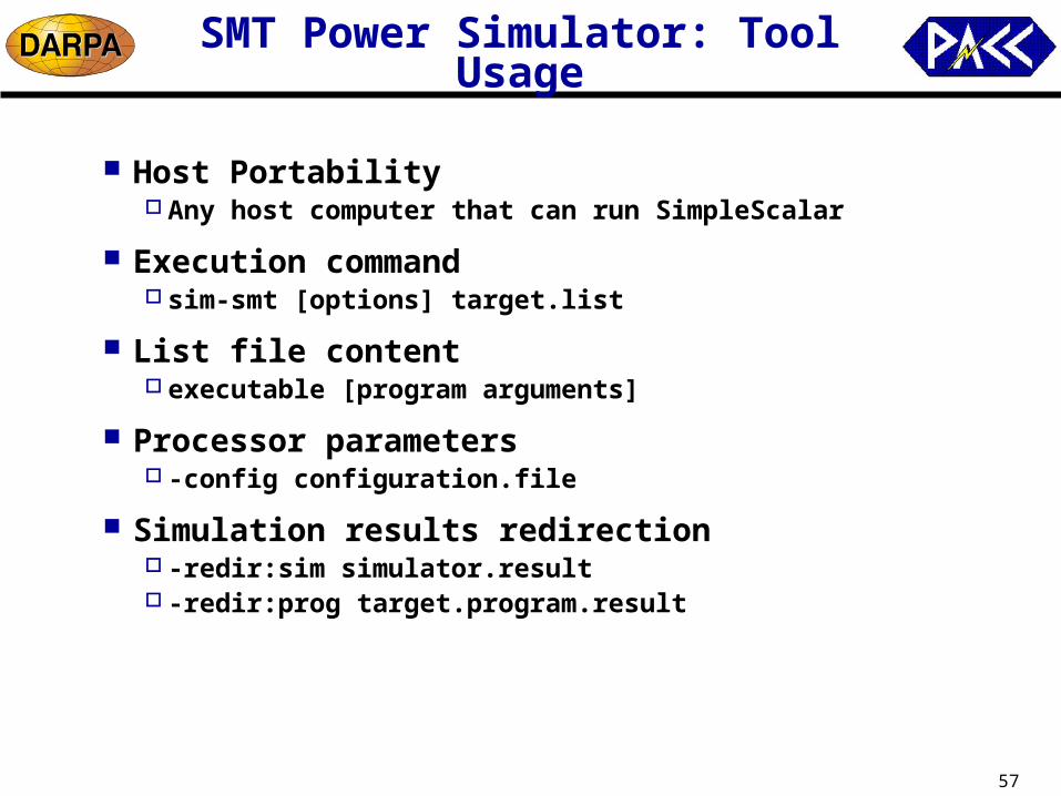
SMT Power Simulator: Tool Usage

Host Portability Any host computer that can run SimpleScalar

Execution command sim-smt [options] target.list

List file content executable [program arguments]

Processor parameters -config configuration.file

Simulation results redirection -redir:sim simulator.result -redir:prog target.program.result

58

Mode Selection

Determine when what component is running at what mode

Mode selection is non-trivial Scheduler will be overwhelmed to determine component modes at the

same time! Exploration space of all mode combinations is tremendous Greedy solution may fail mission timing-constraints or power

constraints

Mode selection is worthwhile Exploration spaces exist to improve power reduction and power-

awareness Energy saving ( 5-15%) Cost saving: (10-40%) Ease the task planning and give a more realistic picture

59

Methodology and Design Flow

The whole picture - the integration of: Power-aware scheduler Mode selector Power estimation/profiling tools

Static view

Scheduler

Power Estimator

Initial schedule

modified schedule

Power/timing numberpower profile Power/timing budget

Power/timing budget

Power profile

Mode Selector

60

System Modeling

Component power model Power modes with overhead

System timing model Constraint graph

Mode dependency modeling Mode dependency graph

External parameters Environment temperature Surrounding terrain

61

Component Power Model

Power mode Each mode is defined by power and timing attributes

Constant, Profile, external (environmental) parameters May be hierarchical -- e..g. PowerPC 7450

active: { cache on: { cache settings }, cache off,voltage scaling, clock scaling },

doze: { clock scaling }, nap: { } deep sleep: { }

Overhead on mode changes Power overhead, timing overhead e.g. preheating a motor, voltage scaling, PLL

Environmental parameters e.g. temperature, terrain (roughness of ground for a motor) Affect power and timing overhead

62

Component Model Examples

Driving motor Power is function of Temperature Mode change time also function

of Temperature T

Microprocessor (PowerPC 603e)

off on0WPower: –0.1225*T + 1.0

Power: 2.2WTime: (–1.875*T+10)*(T<0) +10*(T≥0)

Power: 0.5WTime: 3

Full power

Doze Nap Sleep

DPM4.0W 3.2W

1.0W 70mW 40mW

10 cycles -

10 cycles -

10 cycles -

10 cycles - 100us + 255 bus clocks + 10 cycles

100us + 255 bus clocks + 10 cycles

t1 + 3 cycles3 cycles t1 + 3 cycles

63

FireWire Bus Power Model

Cable Power Pc = µ·L ·Cf (µ: constant, L: cable length, Cf: data transfer rate)

Driver Power (Pd) Fast lookup table Protocol simulator (in progress)

Event-driven system-level simulator Generated event traces for high level power estimation

Bus Power Pbus = Pc + Pd 100MHz 200MHz 400MHz

Full-on 320 mW 350mW 380 mW

Idle 250mW 250mW 250mW

Ultra low power 0.5 mW 0.5 mW 0.5 mW

TSB41AB3 IEEE 1394a-2000 THREE-PORT CABLETRANSCEIVER/ARBITER

64

Design Flow

componentlibrary

scheduler high-levelsimulator

modeselector

powersimulator

task model,timing /powerconstraints

Compiler

power profile,C program

modemodel

power + timingestimation

task allocation,component selection

CO

PP

ER

IMP

AC

CT

low-levelsimulator

executable

65

Timing: Constraint graph

Min/max timing constraints between pairs of events

Vertices Represent events A task has a Start and an End event

e.g. A.s = start event of task A, B.e = end event of task B

Directed edges Weights on edges Nonnegative weight: min constraint Negative weight: -max constraint

A.s B.e10

End event of B should be no earlier than 10 time units after the start event of A

A.s B.s-10

Start event of B should be no later than 10 time units after the start event of A

66

System Timing Modeling Example

Haz.e drv.e5 cam.s1drv.s-10

ppc1.s ppc2.s-20

ppc1.e

sci.s1

rf.e

str.s

1

str.s-5

1

1

-30

Haz: hazard detectorStr: steering motorDrv: driving motorCam: cameraPpc: processorSci: scientific deviceRf : radio frequency modem

Micro Rover example Multiple resources Timing constraints between tasks

67

Mode Dependency Modeling

Functional modes examples: ATR -- short range, middle range behavior choice as dictated by functional requirements

(i.e., not controllable by power management)

Component modes examples: processor full-on, sleep, doze, voltage/clock scaling operational setting of component

(i.e., open to mode selection for meeting power/timing constraints)

Dependencies Among functional modes (of different activities) Among component modes Between functional and component modes

e.g., ATR in short-range mode, Processor running in high-clock rate

68

Mode dependency graph

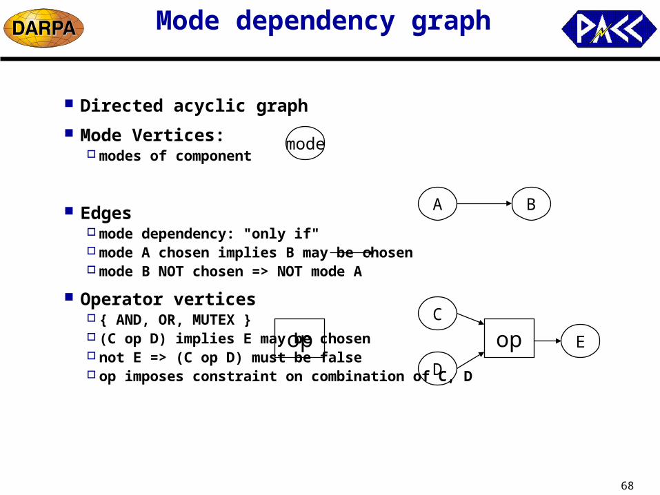
Directed acyclic graph

Mode Vertices: modes of component

Edges mode dependency: "only if" mode A chosen implies B may be chosen mode B NOT chosen => NOT mode A

Operator vertices { AND, OR, MUTEX } (C op D) implies E may be chosen not E => (C op D) must be false op imposes constraint on combination of C, D

A B

C

D

op E

mode

op

69

Mode dependency example: Rover

haz: hazard detectorstr: steering motordrv: driving motor

haz.on

str.ondrv.on

ORMUTEX

Components hazard detector, driving motor,

steering motor

Constraints on modes: hazard detector and the motors should

not be working at the same time

Mode combinations

Hazard detector Driving motor Steering motor

M0 Off Off Off

M1 Off On Off

M2 Off Off On

M3 Off On OnM4 On Off Off

70

Mode Modeling Example:µAMPS sensors

Components: processor, memory, RF, sensor

Constraints on modes: Processor is active when both radio and

sensor is active Memory is active only when processor is

active

Microsensor architecture

S.on

R.onAND

S.on

R.rx XOR

A.sleep

A.active M.on

R.rx_tx

MUTEXA.idle

A.sleep

A:ARMM:memoryR: radioS: sensor

A.activeM.on

71

Mode Modeling of µAMPS sensors(cont’d)

Mode combinations considered: by MIT group: 5 combinations manual grouping, ad hoc

Our method 3 more combinations systematically generated from

dependency graph

Add constraint: When sensor is off, all other component

should be off (proactive)

Automatically obtain same results as MIT group

Mode S R A M

M0 On Tx,rx Active On

M1 On Rx Idle Off

M2 On Rx Sleep Off

M3 On Off Sleep Off

M4 Off Tx,rx Active On

M5 Off Rx Idle Off

M6 Off Rx Sleep Off

M7 Off Off Sleep Off

Not

giv

en b

y M

IT g

rou

pR.on S.on

72

Mode Combination Enumeration- Using Dependency Graph

Component level mode dep. graph Group modes by component Show mode dependency between

components

Enumerating reachable modes Topological sorting Graph helps prune out infeasible

mode combinations

Break cycle in comp. graph Removing an edge in cycle Keep track of the last dependent

successor component

Radio

Sensor

ARM Memory

RadioSensor ARM Memory

off off sleep off

on off sleep off

idle off

on idle off

active on

73

External Parameters & Constraints

Parameters in system model Temperature, terrain Used to characterize

components and their overhead

System Constraints Maximum Power constraint

Constant or power profile (function of time)

Minimum Power constraint Constant or power profile (

function of time) Total energy constraint ( under

working) Mission time (mission deadline)

Temperature (C) Power (W)

0 1.0

-40 5.9

-80 9.6

Power consumption of Driving motor at different temperatures

74

System Power Representation

Schedule Gantt Chart

Time view Power view

Mode selection Gantt chart

Tasks marked with mode settings

Added non-operating tasks Idle intervals mode change

overheads Power profile view

75

Design Flow

componentlibrary

scheduler high-levelsimulator

modeselector

powersimulator

task model,timing /powerconstraints

Compiler

power profile,C program

modemodel

power + timingestimation

task allocation,component selection

CO

PP

ER

IMP

AC

CT

low-levelsimulator

executable

76

Mode selection: Problem statement

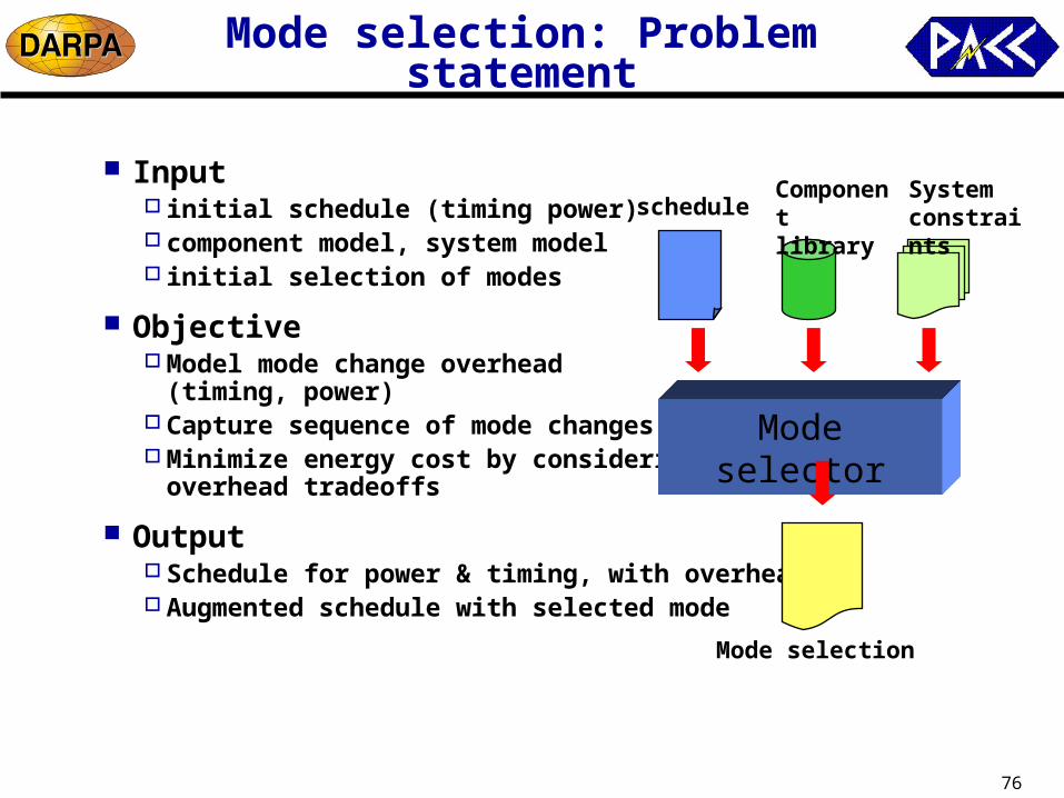
Input initial schedule (timing power) component model, system model initial selection of modes

Objective Model mode change overhead

(timing, power) Capture sequence of mode changes Minimize energy cost by considering

overhead tradeoffs

Output Schedule for power & timing, with overhead Augmented schedule with selected mode

Mode selector

scheduleComponent library

System constraints

Mode selection

77

Application Example: Rover

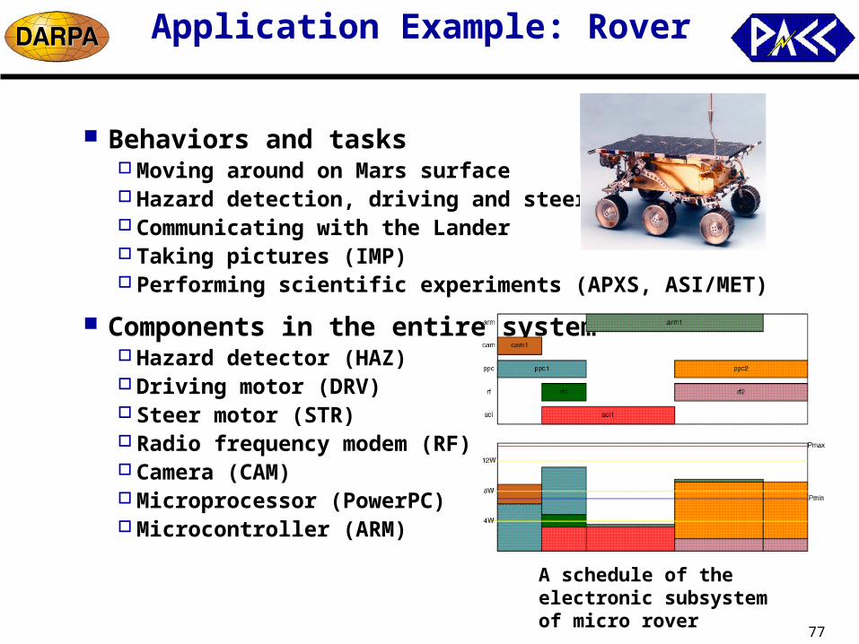
Behaviors and tasks Moving around on Mars surface Hazard detection, driving and steering Communicating with the Lander Taking pictures (IMP) Performing scientific experiments (APXS, ASI/MET)

Components in the entire system Hazard detector (HAZ) Driving motor (DRV) Steer motor (STR) Radio frequency modem (RF) Camera (CAM) Microprocessor (PowerPC) Microcontroller (ARM)

A schedule of the electronic subsystem of micro rover

78

Mode selection Results:Energy savings

Traditional approach Only two modes: { On, Off } Timing constraints ONLY Power constraints may be violated Considers mode change overhead

Our Approach:with Mode Selection All legal mode combinations Both timing and power constraints Detailed mode change overhead

Results Energy saving: 3.7% to 11.9% average saving: 8.7%

1300

1350

1400

1450

1500

1550

1600

1650

1700

1750

5 6 7 8 9 10

Mode SelectionOn&Off

Pmin(W)

Energy(J)

79

Results for mode selection:Cost savings

Cost vs. Energy saving: Cost defined as energy above

minimum constraints

Savings From 6.9% to 49.3% average 26.5%

0

100

200

300

400

500

600

700

800

900

1000

5 6 7 8 9 10

Mode Selection

On&Off

Pmin (W)

Energy (J)

80

Exploring Different Working Scenarios

Three tasks Moving around (MOV) Taking picture (CAM) Scientific experiment (SCI)

Three scenarios A: MOV, CAM, SCI B: CAM, MOV, SCI C: CAM, SCI, MOV

Temperature profile is given as: Temperature

-90

-80

-70

-60

-50

-40

-30

-20

-10

01 2 3 4 5 6

123456

81

Result III

Scenarios consume different amounts of energy Scenario C consumes 12%

more energy than scenario A (by mode selection)

Mode selection always does better compared to (on, off) only up to 11.7% energy saving

0

5000

10000

15000

20000

25000

A B C

Mode SelectionOn&off

82

Mode selection: Issues

Challenges: Explosion of state space -- grows exponentially Modeling restrictions in mode change sequence

Solution / novelty Formalism for mode dependency at component level & system level Systematically prune search space

Experimental results Energy and time saved More accurate modeling of overhead

83

Accomplishments to date

Power-aware scheduling Multi-processor/domain, Min / Max power and timing constraints 3 classes of system level pipelining techniques

Mode selection Component and system model Captures power & timing overhead on mode change

Incorporating power models and simulators SMT simulator for advanced microarchitectural exploration FireWire, DRAM, cache, PowerPC

Tool prototype & Integration GUI for power-aware Gantt chart scheduling & mode selection Power aware visualization tool for benchmarks Interface to COPPER project

84

Lessons learned

Challenges Not all applications fit a given model Alternative design flows may be required for different applications Manually extract parallelism & dependency in benchmarks Capture mode dependency in components & applications Integration of good power models for PowerPC

Right level of abstraction Many low-level power models available; not always usable Need system-level power estimations Details of the architecture model Memory / bus power models Overhead for voltage/frequency scaling

85

Fulfilled Milestones

Power-aware scheduling [3 papers] Multi-scenario System-level pipelining

Mode selection encompass power management (voltage/freq scaling)

UI prototype scheduling, mode selection, benchmark visualization

Initial tool integration interface to COPPER

Processor power & simulation models SMT simulator

86

Upcoming Milestones

Dynamic optimization Scheduling and planning -- using the Deep Impact example Pipeline depth/width tuning at run-time

Additional static optimization component selection/assignment bus topology optimization

Simulation Bus simulation models SMT -- Thermal dissipation profiling,

Dynamic power/thermal management

Tool integration Simulation models from other groups IMPACCT tools and library tighter integration between IMPACCT and COPPER

87

Ideas: dynamic optimization

More dynamic scenarios Power suddenly cut off, with small power reserve before shutdown Mission replanning, changing objectives

Solutions required Division between static preparation & dynamic handling Ability to decide most important actions to take under extreme time

constraint Need feedback/notification mechanism in execution model Decentralized power management

Need new benchmark examples

88

Future planned evaluation

Deep Impact from JPL Mission planning and scheduling example Image compression (wavelet) algorithm Architectural mapping

JPL Testbed PPC750 board to measure actual power PPC750 to simulate instrumentation in real-time advanced board with real instrumentation

Validation through simulation Scheduler output fed to COPPER for compilation Simulation via COPPER and our own SMT Compare estimated power with refined version

89

Applications

Space Mars Rover (scheduling, mode selection) Deep Impact (planning)

UAV DAATR (pipelined scheduling)

(mode selection under investigation)

Distributed sensors MIT µAMPS sensor (mode selection)

Need apps requiring dynamic planning/reconfig!

90

Development plans

Scripting and web-based tool Jython (Java + Python), TkInter for GUI prototype Core scheduler

Modular, detachable from GUI Option to run on separate server or same process as UI

CGI scripts for arch. configuration (unix/web based) Latest version distributed thru WebCVS

Interface with commercial CAD backend Detailed power estimation tools Functional simulation with proprietary models

Rationale Open source, runs on any platform All publicly available development tools Trivial to install, no compilation, encourage modification

91

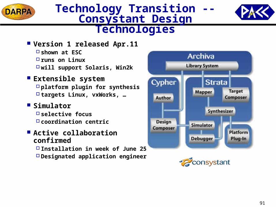
Technology Transition --Consystant Design Technologies

Version 1 released Apr.11 shown at ESC runs on Linux will support Solaris, Win2k

Extensible system platform plugin for synthesis targets Linux, vxWorks, …

Simulator selective focus coordination centric

Active collaboration confirmed Installation in week of June 25 Designated application engineer

92

http://www.ece.uci.edu/impacct/

93

Metrics

Source-aware energy model Takes “free energy” into account Cost for not using free energy

Profile-aware Total energy dependent on consumers’ power profile Smoothness of power draw

Scenario-aware Cost function tracks external factors (e.g. temperature, solar level) Stage in mission

Timing/performance Makespan (length of an iteration) Dynamic planning cost

94

Architectural Configuration

Mode selection Power consumption level (doze, nap, sleep, etc.) Low power design techniques

Clock scaling, voltage scaling Memory/cache configurations, bus encoding Communication protocols, compression, algorithm transformations

Optimize feasible solutions for energy/timing costs Power, Real time, Inter-resource modes constraints Constraints between functionality modes and resources modes

Functionality mode and resource modes

Bus topology optimization Static clustering and bus partitioning Dynamic reclustering with shutdown

95

Application - Mars Rover

Mission-critical embedded system Hard real-time system Composed of COTS component

Electronic: µprocessor, µcontroller, memory,camera, scientific devices, ... Mechanics/thermal: driving motor, steering motor, heaters, … Power sources: solar panel, battery

Power/energy and performance constraints Stringent max power constraint Flexible min power constraint Limited non-rechargeable energy sources Global timing requirement

Limited working window during sol daytime Timing constraint among tasks

Harsh and uncertain working environment Extremely low temperature - affects component behaviors Uncertain environment: winds/obstacles/rugged terrain

96

Example Platform- X2000

COTS components Modeling Processors (PowerPC 603e, 750) Memory organization (cache, memory) System interconnects (FireWire bus driver/controller) Scientific equipment Sensors/actuators Mechanics/Thermals (driving/steering motors/heaters)

System-level architecture modeling Tree topology for FireWire bus architecture Component clustering for bus segmentation

97

Testing Methodologies

A "Activity" for given duration (5 s, 10 s, 15 s) repeated 6 times record both I-cache & D-cache misses (recorded in separate runs)

B Recording 90 seconds worth of an Activity till its completion 1 minute gap between runs also I-cache & D-cache misses

C -- what is measurement C?

98

User Input

Attributes tasks, resources, timing constraints, power budgets

Unique features power as constraint scheduling, system-level mission planning, power-aware loop

pipelining, timing constraint classification. subsumes deadline, dataflow

Language mix of graphical and custom constraint language

99

Methodology and Work Flow

Exploration techniques Backtracking Cutting exploration space with multi-dimensional constraints

Two steps in design exploration: Find feasible mode selection for operating tasks

Timing constraints Constraint graph Resource slacks Mission deadline

Dependency between tasks Dependency graph

Find feasible mode selections for idle intervals System power/energy constraints: min, max, or power profile Mode change overhead, both time and power overheads

Speedup techniques Sorting component modes with power numbers