integrated land capability for ecological sustainability of on-site … · 2010-06-09 · wael r....

Integrated Land Capability for

Ecological Sustainability of On-site

Sewage Treatment Systems

Wael R. Al-Shiekh Khalil

BSc Eng. (WVU), M Eng. (QUT)

A THESIS SUBMITTED TO THE SCHOOL OF CIVIL

ENGINEERING

QUEENSLAND UNIVERSITY OF TECHNOLOGY

IN PARTIAL FULFILLMENT OF THE REQUIREMENTS OF

THE DEGREE OF DOCTOR OF PHILOSOPHY

FACULTY OF BUILT ENVIRONMENT AND ENGINEERING

September 2005

i

Statement of Original Authorship

The work contained in this thesis has not been previously submitted for a degree

or diploma for any other higher education institution to the best of my knowledge

and belief. The thesis contains no material previously published or written by

another person except where due reference is made.

Signed:

Wael R. Al-Shiekh Khalil

Date: / /

ii

Abstract

The research project was formulated to solve serious environmental and possible

public health problems in rural and regional areas caused by the common failure

of soil disposal systems used for application of effluent from on-site domestic

sewage treatment systems. On-site sewage treatment systems adopt a treatment

train approach with the associated soil disposal area playing a crucial role. The

most common on-site sewage treatment system that is used is the conventional

septic tank and subsurface effluent disposal system. The subsurface effluent

disposal area is given high priority by regulatory authorities due to the significant

environmental and public health impacts that can result from their failure. There is

generally very poor householder maintenance of the treatment system and this is

compounded by the failure of the effluent disposal area resulting in unacceptable

surface and groundwater contamination. This underlies the vital importance of

employing reliable science-based site suitability assessment techniques for

effluent disposal. The research undertaken investigated the role of soil physico-

chemical characteristics influencing the behaviour of effluent disposal areas.

The study was conducted within the Logan City Council area, Queensland State,

Australia. About 50% of the Logan region is unsewered and the common type of

on-site sewage treatment used is a septic tank with subsurface effluent disposal

area. The work undertaken consisted of extensive field investigations, soil

sampling and testing, laboratory studies and extensive data analysis.

In the field study, forty-eight sites were investigated for their effluent application

suitability. The sites were evaluated based on the soil physico-chemical

characteristics. The field investigation indicated that there were nine soil orders in

the study area. These soil orders were Dermosols, Chromosols, Kandosols,

Kurosols, Vertosols, Sodosols, Tenosols, Rudosols and Anthrosols. The soils in

all the investigated sites were acidic soils in the pH range between 5 and 6.5.

The complexity of the large data matrix obtained from the analysis was overcome

by multivariate analytical methods to assist in evaluating the soils’ ability to treat

iii

effluent and to understand the importance of various parameters. The analytical

methods selected to serve this purpose were PROMETHEE and GAIA. The

analysis indicated that the most suitable soils for effluent renovation are the

Kandosols whilst the most unsatisfactory soil order was found to be Podosol. The

GAIA analysis was in agreement with quantitative analysis conducted earlier.

An extensive laboratory column study lasting almost one year was undertaken to

validate the results of the data analysis from the field investigation. The main

objectives of this experiment were to examine the soil behaviour under practical

effluent application and to investigate the long-term acceptance rate for these

soils. Twelve representative soils were selected for the column experiment from

the previously investigated sites and undisturbed soil cores were collected for this

purpose. The results from the column study matched closely with the evaluation

conducted at the earlier stages of the research. Soil physico-chemical analysis

before and after effluent application indicated that the soils’ acidity was improved

toward neutrality after effluent application. The results indicated that soils have a

greater ability to handle phosphorus than nitrogen. The most favorable cation

exchange capacity for soils to treat and transmit effluent was between 15 and 40

meq/100g.

Based on the results of the column study, the long-term acceptance rate (LTAR)

was determined for the investigated twelve soil types. Eleven out of twelve soils

reported specific LTAR values between 0.18-0.22 cm/day. For the duration of the

laboratory study, the Podosol order did not reach its LTAR value due to the

extremely sandy nature of the soil. The time required to achieve LTAR varied

between different soils from 40 to 330 days.

The outcomes of this research was integrated into a soil suitability map for on-site

sewage treatment systems for Logan City Council. This will assist the authorities

in providing sustainable solutions for on-site systems failure.

iv

List of Publications Peer Reviewed Journal Papers

• W. Al-Shiekh Khalil, A. Goonetilleke, S. Kokot and S. Carroll. 2004. Use of

chemometrics method and multicriteria decision making for site selection for

sustainable on-site sewage effluent disposal. J. Analytica Chimica Acta, Vol.

506, pp.41-56.

• W. Al-Shiekh Khalil, A. Goonetilleke and J. T. Kloprogge. 2004. Use of

multivariate analysis to understand the significant of CEC, organic matter and

pH on the soil capacity for adsorption of effluent contaminants. J.

Environmetrics (In press).

• S. Carroll, A. Goonetilleke, W. Al-Shiekh Khalil and R. Frost. 2004.

Assessment of soil suitability for effluent renovation using undisturbed soil

columns. Gederma. (In press).

Peer Reviewed Conference Papers

• W. Al-Shiekh Khalil and A. Goonetilleke. 2002. Integrated land capability for

ecological sustainability of onsite sewage treatment systems. In Proceedings of

the 9th Bi-Annual PIC Postgraduate conference, PIC. June 2002. School Of

Civil Engineering, QUT, Australia,.

• W. Al-Shiekh Khalil, A. Goonetilleke and R. Frost. 2002. Use of soil physical

and chemical data for evaluating the long-term sustainability of subsurface

effluent disposal systems. In Proceedings of the 5th International Conference

on Coasts, Ports and Marine Structures. Ramsar-Iran. 313-318.

• W. Al-Shiekh Khalil, A. Goonetilleke and Les Daws. 2003. Correlation of soil

data with treatment performance of subsurface effluent disposal systems. In

Proceedings of the On-site ‘03 Conference, Armidale, NSW.

• W. Al-Shiekh Khalil, A. Goonetilleke and Portia Rigby. 2004. Use of

undisturbed soil columns to evaluate soil capability to renovate on-site sewage

treatment effluent. In Proceedings of the Tenth National Symposium on

Individual and Small Community Sewage Systems. Sacramento, California,

U.S.A. 202-209.

v

Acknowledgements

I wish to express my appreciation to my Principal Supervisor A/Prof. Ashantha

Goonetilleke for his guidance, support and professional advice given to me over

the duration of this study. Special thanks is also given to my Associate Supervisor

Dr Theo Kloprogge for his guidance and professional support through the stages

of the research.

Appreciation is extended to Mr Tony Raftery for his technical support in the X-

ray diffraction analysis. Also, special thanks to Mr Bill Kwiecien for his technical

support in ICP-OES and AAS analysis. Appreciation is extended to all staff in the

School of Civil Engineering and special thanks to my colleagues Steven Carroll

and Les Dawes, School of Physical and Chemical Science, especially Wade

Martens.

I wish to express my thanks to the staff of Logan City Council for the support

through the stages of the study, especially:

Mr Shane Mansfield Regulatory Services Manager

Mr Steven Keks Special Projects Coordinator

Mr Peter George Principal Plumbing Inspector

Dr Michelle Mills Waterways officer

Mr Jan Cilliers Senior Strategic Planning Officer

Mr Greg Bird Senior Water & Sewerage Control Officer

I wish to express my gratitude and appreciation to my father (Al-Haj Ramadan

Hamed) and mother (Al-Haja Eidah) for their unlimited support and sacrifices and

love. I would also like to thank my brothers and sisters and my father-in-law (Abd

Al-Star) and his family.

vi

Dedication

In acknowledgement of the loving support and constant encouragement extended

to me, I dedicate this thesis to my loving wife Diana and my lovely children

Ramadan, Bashar and Razan.

vii

Table of Contents

Statement of Original Authorship...................................................... i

Abstract .......................................................................................... ii

List of Publications............................................................................. iv

Acknowledgements.............................................................................. v

Dedication ......................................................................................... vi

Abbreviations .................................................................................. xvii

Chapter 1 Introduction .................................................................. 1

1.1 Overview..................................................................................................1

1.2 Project Aims and Objectives....................................................................1

1.3 Hypotheses ...............................................................................................2

1.4 Scope........................................................................................................2

1.5 Justification for the Research...................................................................3

1.6 Project Area .............................................................................................3

1.7 Methodology for the Study ......................................................................7

1.8 Outline of the Thesis ................................................................................8

Chapter 2 On-site Sewage Treatment: Chemical and Biological

Interactions in Soils .................................................................... 10

2.1 Overview................................................................................................10

2.2 Treatment System Performance .............................................................11

2.3 Hydraulic Performance ..........................................................................14

2.4 Mechanisms of Clogging .......................................................................17

2.5 The Soil as a Treatment Medium...........................................................20

2.5.1 Soil Definition and Composition ...................................................21

2.5.2 Mineralogy of the Clay Fraction....................................................24

2.5.3 Soil Profiles....................................................................................28

2.5.4 Soil Classification ..........................................................................29

2.5.5 Chemical Reactions .......................................................................33

2.5.6 Interaction of Water with Soils ......................................................35

viii

2.6 Transport of Effluent Pollutants in Soil and Groundwater.................... 36

2.6.1 Solids (Suspended Solids and Dissolved Solids) .......................... 37

2.6.2 Nutrients (Nitrogen and Phosphorus) ............................................ 37

2.7 Conclusions ........................................................................................... 49

Chapter 3 Analytical Procedures ..................................................51

3.1 Introduction ........................................................................................... 51

3.2 Soil and Effluent Analysis..................................................................... 52

3.2.1 pH .................................................................................................. 52

3.2.2 Electrical Conductivity .................................................................. 53

3.2.3 Chloride Ions ................................................................................. 53

3.2.4 Organic Matter Content ................................................................. 54

3.2.5 Total Nitrogen................................................................................ 55

3.2.6 Phosphorus..................................................................................... 58

3.2.7 Cation Exchange Capacity............................................................. 59

3.2.8 X-ray diffraction (XRD)................................................................ 60

3.2.9 Exchangeable Cations (Mg2+, Al3+, K+, Fe2+, Ca2+, Na+) .............. 62

3.2.10 Chemical Oxygen Demand of Effluent ......................................... 62

3.3 Chemometrics and Multi-criteria Decision Making.............................. 63

3.3.1 Chemometrics................................................................................ 63

3.3.2 Common (MCDM) Methods ......................................................... 64

3.3.3 PROMETHEE Applications.......................................................... 65

3.3.4 GAIA ............................................................................................. 68

3.4 Conclusions ........................................................................................... 69

Chapter 4 Characterisation of the Soil Types.............................70

4.1 Introduction ........................................................................................... 70

4.2 On-site Wastewater Treatment Systems in the Logan City Region ...... 70

4.3 Site Selection Process............................................................................ 71

4.3.1 Desktop Study................................................................................ 73

4.3.2 Field Investigations........................................................................ 75

4.4 Soil Sampling ........................................................................................ 81

4.4.1 Procedures ..................................................................................... 81

ix

4.4.2 Sample Preparation and Handling..................................................82

4.5 Evaluation of the Soils Investigated ......................................................85

4.6 Description of Soil Orders .....................................................................88

4.6.1 Dermosol Soil ................................................................................88

4.6.2 Chromosol Soil ..............................................................................90

4.6.3 Kandosol Soil.................................................................................91

4.6.4 Kurosol Soil ...................................................................................92

4.6.5 Vertosol Soil ..................................................................................93

4.6.6 Sodosol Soil ...................................................................................94

4.6.7 Rudosol Soil...................................................................................94

4.6.8 Bleached-Leptic Tenosol ...............................................................95

4.6.9 Spolic Anthroposol ........................................................................95

4.7 Conclusions............................................................................................96

Chapter 5 Experimental Study on Vertical Effluent Transport in

Soils ........................................................................................ 99

5.1 Overview................................................................................................99

5.2 Objectives ..............................................................................................99

5.3 Justification ............................................................................................99

5.4 Design ..................................................................................................100

5.5 Laboratory Columns - Manufacture and Preparation ..........................102

5.6 Soil Cores Collection ...........................................................................103

5.7 Soil Columns - Preparation and Handling ...........................................107

5.8 Effluent Application and Sampling .....................................................109

5.9 Description of the Soil Cores ...............................................................112

5.10 Soil Characterisation............................................................................116

5.10.1 Mineralogical Analysis ................................................................116

5.10.2 Organic Matter Content ...............................................................121

5.10.3 Cation Exchange Capacity ...........................................................124

5.10.4 pH.................................................................................................127

5.10.5 Electrical Conductivity ................................................................130

5.10.6 Chloride Ion .................................................................................133

5.10.7 Nutrients (P and N ) .....................................................................137

x

5.10.8 Exchangeable Cations (Al3+, Fe2+, Mg2+, Na+, Ca2+ and K+) ...... 143

5.10.9 Ca:Mg Ratio and Exchangeable Sodium Percentage (ESP)........ 147

5.11 Effluent Analysis ................................................................................. 153

5.11.1 Column 1 (Yellow Kurosol) ........................................................ 153

5.11.2 Column 2 (Hydrosol)................................................................... 157

5.11.3 Column 3 (Podosol)..................................................................... 159

5.11.4 Column 4 (Black Sodosol) .......................................................... 162

5.11.5 Column 5 (Red Dermosol) .......................................................... 164

5.11.6 Column 6 (Brown Kurosol)......................................................... 166

5.11.7 Column 7 (Brown Vertosol) ........................................................ 168

5.11.8 Column 8 (Brown Dermosol) ...................................................... 170

5.11.9 Column 9 (Yellow Dermosol) ..................................................... 172

5.11.10 Column 10 (Yellow Chromosol) ................................................. 174

5.11.11 Column 11 (Grey Chromosol)..................................................... 176

5.11.12 Column 12 (Red Kandosol)......................................................... 178

5.12 Conclusions ......................................................................................... 180

Chapter 6 Data Analysis and Validation ..................................182

6.1 Overview ............................................................................................. 182

6.2 Evaluation Based on Soil’s CEC......................................................... 183

6.3 Multicriteria Decision Making Methods for Sites Ranking ................ 185

6.4 Long Term Acceptance Rate (LTAR) ................................................. 197

6.4.1 LTAR for Soil Cores ................................................................... 198

6.4.2 Example for the k Value Calculation .......................................... 199

6.4.3 Soil Percolation Rate and LTAR................................................. 200

6.4.4 Behaviour of Individual Columns ............................................... 202

6.4.5 Summary of Observations ........................................................... 214

6.5 Sites Evaluation Validation ................................................................. 215

Chapter 7 Conclusions and Recommendations ........................220

7.1 Site Evaluation Based on Soils’ Physico-chemical Characteristics .... 220

7.2 Site Evaluations Using Multivariate Analysis..................................... 220

7.3 Soil Column Study............................................................................... 221

xi

7.4 Long-term Acceptance Rate.................................................................224

7.5 Recommendations................................................................................225

Chapter 8 References................................................................... 226

Appendix A Soil Data from the Field Investigation .................... 245

Appendix B Experimental Columns Data .................................... 258

Appendix C Checklists for Field Sampling .................................. 292

xii

List of Figures

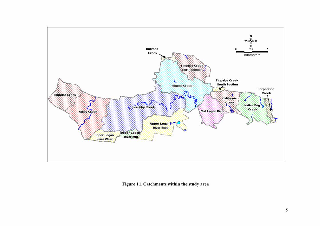
Figure 1.1 Catchments within the study area ..........................................................5

Figure 1.2 Catchments within the study ..................................................................6

Figure 2.1 Schematic diagram of a septic system (adapted from AS/NZS

1547:2000).....................................................................................................10

Figure 2.2 Effective infiltrative subsurface area (A+B+C) and location of the

clogging layer in the soil trenches .................................................................12

Figure 2.3 Typical cross section for effluent transport zones in subsurface effluent

disposal treatment system..............................................................................12

Figure 2.4 Approximate percentages of constituents in soils (Bridges, 1978)......22

Figure 2.5 Silicon tetrahedron ...............................................................................26

Figure 2.6 Aluminium octahedron.........................................................................26

Figure 2.7 Schematic diagrams: A) kaolinite (1:1) clay structure, B) illite (2:1)

clay structure and C) the expanding clay smectite (2:1) ...............................27

Figure 2.8 Nitrogen gas transformations in an on-site sewage treatment system .39

Figure 4.1 On-site systems in the study area .........................................................72

Figure 4.2 Planning scheme sensitivity zones for Logan City Council region .....76

Figure 4.3 Location of the preliminary and detailed investigation sites ...............80

Figure 4.4 Example of soil sampling, showing soil auger sample layout and

sample bags....................................................................................................83

Figure 4.5 Example of measuring the average soil sampling depth......................84

Figure 4.6 Example of a soil profile used to match with the Australian Soil

Classification .................................................................................................85

Figure 5.1 Schematic diagram for a typical laboratory column ..........................102

Figure 5.2 Columns placed on a trolley...............................................................103

Figure 5.3 Photo presents the drilling auger with the hollow auger inside .........105

Figure 5.4 Process of collecting the soil from the hollow auger .........................105

Figure 5.5 Soil core after collection ....................................................................106

Figure 5.6 Soil core shows distinct A and B-horizons ........................................106

Figure 5.7 Column preparation............................................................................108

Figure 5.8 Four columns after the setting is completed ......................................108

xiii

Figure 5.9 The method of soil column feeding................................................... 109

Figure 5.10 Effluent drip-feeding ....................................................................... 110

Figure 5.11 The collection of the discharged effluent ........................................ 111

Figure 5.12 Complete soil column experiments setting for the twelve columns 111

Figure 5.13 Approximate location of soil cores in a hypothetical hydrological

catena .......................................................................................................... 115

Figure 5.14 Mineralogical analysis for Columns 1, 2, 3 and 4 ........................... 117

Figure 5.15 Mineralogical analysis for Columns 5, 6, 7 and 8 ........................... 119

Figure 5.16 Mineralogical analysis for Columns 9, 10, 11 and 12 ..................... 120

Figure 5.17a OM soil in Columns1, 2, 3 and 4................................................... 122

Figure 5.17b OM soil in Columns 5, 6, 7 and 8.................................................. 122

Figure 5.17c OM soil in Columns 9, 10, 11 and 12............................................ 123

Figure 5.18a CEC soil in Columns 1, 2, 3 and 4 ................................................ 125

Figure 5.18b CEC soil in Columns 5, 6, 7 and 8 ................................................ 126

Figure 5.18c CEC soil in Columns 9, 10, 11 and 12 .......................................... 127

Figure 5.19a Soil pH in Columns 1, 2, 3 and 4................................................... 128

Figure 5.19b Soil pH in Columns 5, 6, 7 and 8 .................................................. 129

Figure 5.19c Soil pH in Columns 9, 10, 11 and 12............................................. 130

Figure 5.20a EC level in Columns 1, 2, 3 and 4 ................................................. 131

Figure 5.20b EC level in Columns 5, 6, 7 and 8 ................................................. 132

Figure 5.20c EC level in Columns 9, 10, 11 and 12 ........................................... 132

Figure 5.21a Cl- in soil Columns 1, 2, 3 and 4.................................................... 135

Figure 5.21b Cl- in soil Columns 5, 6, 7 and 8 ................................................... 136

Figure 5.21c Cl- in soil Columns 9, 10, 11 and 12.............................................. 136

Figure 5.22a P for soil Columns 1, 2, 3 and 4 .................................................... 138

Figure 5.22b P for soil Columns 5, 6, 7 and 8 .................................................... 138

Figure 5.22c P for soil Columns 9, 10, 11 and 12 .............................................. 139

Figure 5.23a N for soil Columns 1, 2, 3 and 4.................................................... 141

Figure 5.23b N for soil Columns 5, 6, 7 and 8.................................................... 142

Figure 5.23c N for Columns 9, 10, 11 and 12..................................................... 143

Figure 5.24 Exchangeable cations in Columns 1, 2, 3 and 4 .............................. 145

Figure 5.25 Exchangeable cations in Columns 5, 6, 7 and 8 .............................. 146

Figure 5.26 Exchangeable cations in Columns 9, 10, 11 and 12 ........................ 147

Figure 5.27a Ca:Mg ratio for Columns 1, 2, 3 and 4 .......................................... 148

xiv

Figure 5.27b Ca:Mg ratio for Columns 5, 6, 7 and 8 ..........................................149

Figure 5.27c Ca:Mg ratio for Columns 9, 10, 11 and 12.....................................149

Figure 5.28a ESP for Columns 1, 2, 3 and 4 ......................................................151

Figure 5.28b ESP for Columns 5, 6, 7 and 8 ......................................................152

Figure 5.28c ESP for Columns 9, 10, 11 and 12 ................................................153

Figure 5.29 (A and B) Contaminant removal by soils in Column 1....................155


Figure 5.31 (A, B, C and D) Contaminant removal by soils in Column 3 ..........160

Figure 5.32 Contaminant removal by soils in Column 4.....................................162






Figure 5.38 (A and B) Contaminant removal by soils in Column 10..................175

Figure 5.39 Contaminant removal by soils in Columns 11 .................................177

Figure 5.40 (A, B and C) Contaminant removal by soils in Column 12 .............179

Figure 6.1 GAIA analyses for the selected eight sampling sites, ▲= Soil site

objects; soil parameter criteria; pi (π), decision-making axis. ...........190

Figure 6.2 GAIA analyses for the sixteen sampling sites (from second matrix);

the eight added objects; other labels are as in Figure 6.1. ...........................193

Figure 6.3 GAIA analyses for the forty-eight sampling sites (third matrix). the

remaining 32 soil sites; other labels as in Figures 6.2 and 6.1. ...................195

Figure 6.4 LTAR for columns 1, 2, 3 and 4 ........................................................211

Figure 6.4 LTAR for columns 5, 6,7 and 8 .........................................................212

Figure 6.4 LTAR for columns 9, 10, 11 and 12 ..................................................213

Figure 7.1 Soil treatment ability map for on-site sewage treatment....................223

xv

List of Tables

Table 2.1 Different size fractions of soils (Bridges, 1978)................................... 22

Table 2.2 Cation exchange capacities and surface charge densities for some of the

clay minerals as reported by White (1997) ................................................... 25

Table 2.3 Classifications of World Soils by Robinson (1947) ............................. 30

Table 2.4 Australian Soil Classification (Isbell, 1996; Jacquier et al., 2000) ...... 32

Table 2.5 Concentrations of Pathogens in Effluent as reported by Crites and

Tchobanoglous (1998) .................................................................................. 48

Table 3.1 List and shapes of preference functions (modified by Khalil et al., 2004)

....................................................................................................................... 68

Table 4.1 Sensitivity criteria for Planning Scheme sensitivity map ..................... 74

Table 4.2 Site location and GPS coordinates for the preliminary investigation

stage .............................................................................................................. 78

Table 4.3 Location of the selected sites in the detailed stage ............................... 79

Table 4.4 Soil orders noted in the research area ................................................... 89

Table 4.5 Summary of the main investigated soil descriptions ............................ 97

Table 5.1 Experimental design for the column study ......................................... 101

Table 5.2 Soil columns and field observations ................................................... 113

Table 5.3 Summary of findings for the Yellow Kurosol (Column 1)................. 157

Table 5.4 Summary of findings for the Hydrosol soil ........................................ 159

Table 5.5 Summary of findings for the Podosol soil ......................................... 161

Table 5.6 Summary of findings for the Black Sodosol soil ................................ 164

Table 5.7 Summary of findings for the Red Dermosol Soil ............................... 166

Table 5.8 Summary of findings for the Brown Kurosol Soil.............................. 168

Table 5.9 Summary of findings for Brown Vertosol Soil................................... 170

Table 5.10 Summary of findings for the Brown Dermosol Soil......................... 172

Table 5.11 Summary of findings for the Yellow Dermosol Soil ........................ 174

Table 5.12 Summary of findings for the Yellow Chromosol Soil (Column 10) 176

Table 5.13 Summary of findings for the Grey Chromosol Soil.......................... 178

Table 5.14 Findings for the Red Kandosol Soil.................................................. 180

Table 6.1 Soil classification based on CEC level available on each site. ........... 184

xvi

Table 6.2 Data required for ranking by PROMETHEE ......................................189

Table 6.3 PROMETHEE ranking of the selected eight sampling sites ...............189

Table 6.4 PROMETHEE ranking of the selected sixteen sampling sites............192

Table 6.5 PROMETHEE ranking of the forty-eight sampling sites....................194

Table 6.6 Calculation steps for Column 1 (Yellow Kurosol)..............................200

Table 6.7 Twelve soil columns mineralogy and data ..........................................203

Table 6.8 LTAR for the twelve columns at the first sampling point...................214

Table 6.9 Soils evaluation from the three stages .................................................219

xvii

Abbreviations Al3+

Ca2+

CEC

Cl-

COD

EC

Fe2+

GIS

GPS

K+

LCC

LTAR

Mg2+

MPN

Na+

NH4+

NO3-

OM

PO43-

SSPR

N

P

XRD

Aluminum ion

Calcium cation

Cation Exchange Capacity

Chloride ion

Chemical Oxygen Demand

Electrical Conductivity

Iron as ferrous ion

Geographic Information System

Global Positioning System

Potassium cation

Logan City Council

Long-term Acceptance Rate

Magnesium cation

Most Probable Number

Sodium cation

Ammonium

Nitrate

Organic Matter Content

Orthophosphate

Saturated Soil Percolation Rate

Nitrogen

Phosphorus

X-ray Diffraction

1

Chapter 1 Introduction

1.1 Overview This research project was formulated to identify serious environmental and

possible public health problems caused by the high failure rate of on-site sewage

treatment systems, particularly septic tanks. Due to their low technology and low

cost, septic tank systems are quite often the most appropriate option available for

rural and regional areas. Septic tanks consist of three primary components,

namely an anaerobic chamber, effluent trenches and the subsurface effluent

disposal area below the trenches. Failure of the subsurface disposal area could

occur due to several reasons, such as poor septic tank maintenance, shallow depth

of the subsurface layer and weak physico-chemical characteristics of the soil.

This failure underlies the critical importance in undertaking reliable site suitability

assessment for effluent disposal.

The focus of this research was the subsurface soil disposal area where important

effluent treatment processes take place. Soil in the subsurface area can be very

effective in treating and accommodating the discharged effluent, if the soil

physico-chemical characteristics are suitable for such effluent application. On the

other hand, the failure of the soil to provide the required effluent renovation

processes, or the soil’s low permeability, could result in partially treated sewage

effluent reaching water sources leading to adverse impacts on human health

and/or the environment.

1.2 Project Aims and Objectives The major aim of this study was to evaluate the ability of different soil types to

treat the on-site effluent discharged to the subsurface disposal area. In addition,

the project aimed at assessing the impact of effluent application on the soils’

physico-chemical characteristics. In summary, the aims of the study were:

1. to obtain an in-depth of understanding for the soils in the research area;

2. to examine the soil performance under effluent application; and

3. to evaluate soils’ ability for sewage effluent renovation based on the soil

physico-chemical factors.

2

The objectives of the study were:

1. to validate the soil evaluation based on the physico-chemical analysis with the

actual soil performance;

2. to examine the long–term acceptance rate for the representative soils in the

research area; and

3. to integrate the soil data and knowledge into a soil suitability map for on-site

sewage treatment systems for the Logan City Council region.

1.3 Hypotheses

• Processes influencing effluent renovation are location specific due to

dependency on site, topography, hydrogeology, surface and subsurface soil

characteristics.

• Understanding soil physico-chemical characteristics can assist in predicting

the effluent renovation ability of soil.

1.4 Scope The focus of this research was the subsurface soil disposal area where a

significant fraction of the effluent treatment activity occurs. The research

investigated the soil ability to treat and transmit effluent on individual sites within

the research area. The research was confined to the Logan City Council area, but

the outcomes are applicable anywhere. The study focused on areas which are not

serviced by a centralised sewer system. The knowledge derived from the field

investigation was validated based on a laboratory study of soils under effluent

application. The project specifically focused on the performance of subsurface

effluent disposal systems subjected to the discharge of septic tank effluent.

Aerobic treatment systems and surface disposal of effluent were not investigated.

Additionally, the performances of septic tanks associated with each selected

system were not investigated.

The field study was primarily based on the information obtained from the

available literature. There were forty-eight sites selected in the study area. One

hundred and thirty-nine soil samples were collected from the various soil depths

and analysed for their physico-chemical characteristics. There were gaps in the

3

soil evaluation process which was based on soil phyisco-chemical parameters. A

column study was designed to fill the knowledge gaps in the soil evaluation and to

examine the soils’ performance under effluent application. Most representative

soils in the study area were selected for the column experiment.

1.5 Justification for the Research Septic tanks are the most common form of on-site treatment systems available for

use in rural and regional areas. Septic tanks have high failure rates which can lead

to serious environmental and public health problems. Many reasons cause these

systems to fail such as poor maintenance, shallow depth of the subsurface layer

and weak soil physico-chemical characteristics. In the case of a failed on-site

system, effluent pollutants such as phosphorus, nitrogen and pathogenic bacteria

will be discharged in large quantities to the water body where they could

potentially be transferred to humans through consumption of water and food.

This study was formulated based on scientific research to assist local authorities in

predicting and preventing such problems. The research approached the failure

problem through study of soil physico-chemical characteristics and examined the

ability of different soils to treat and transmit effluent. The outcomes of this

research was integrated into a performance based planning code for Logan City

Council. This will assist the authorities in developing sustainable solutions for

on-site systems failure.

1.6 Project Area The study was carried out within the political boundaries of the Logan City

Council, Queensland State, Australia. Within Logan City, 10% of the total

population is serviced by on-site sewage treatment systems. The city is bordered

by four local authority areas, the City of Brisbane located to the north-west, the

Redland Shire to the north-east, Beaudesert Shire to the south-west and the City of

Gold Coast to the south-east as shown in Figure 1.1.

The research was undertaken within eleven of the fourteen catchments of Logan

City. These included Scrubby Creek, Upper Logan River Mid catchment, Upper

Logan River East catchment, Upper Logan River West catchment, Mid Logan

4

River catchment, Serpentine Creek catchment, California Creek catchment,

Native Dog Creek catchment, Tingalpa Creek South catchment, Tingalpa Creek

North catchment and Slacks Creek catchment. Figure 1.1 shows the catchments.

Given the objectives of this study, all research was undertaken within the

unsewered area. Such areas make up 50% of the total Logan City region. The

areas are mainly concentrated within the southern and eastern suburbs with minor

areas in the north-west. The investigated suburbs are shown in Figure 1.2.

The study included suburbs located on the southside of Logan City, namely:

• Waterford West (Logan Reserve area between School Road, Chambers Flat

and Logan River);

• Park Ridge (between Koplick Road, Rosia Road, Mt Lindsay Highway,

Green Road, Bumstead Road and Chambers Flat); and

• Greenbank (between Andrew Road, Moody Road, Hunter Road, Crest Road

and the Mt Lindsay Highway).

The suburbs located to the east of Logan City included:

• Cornubia; and

• Carbrook (between West Mt Cotton Road, Redland Bay and the city borders

with Redland Shire).

The suburbs located in the west included:

• Hillcrest; and

• Forestdale (between Middle Road, Johnson Road and the border of the

Greenbank Military Camp).

The suburbs located to the north included:

• Berrinba (between Wembley Road, Bardon Road and the Fifth Avenue

area);

• Priestdale; and

• Daisy Hill.

5

Figure 1.1 Catchments within the study area

6

Figure 1.2 Catchments within the study

7

1.7 Methodology for the Study The objectives of the research project were achieved through the following steps:

• Site Selection

The land capability assessment was conducted on the unsewered area under

Logan City Council jurisdiction. The preliminary site selection was based on:

1. the available soil and topographic maps;

2. identification of environmentally sensitive areas such as those located close

to watercourses; and

3. strategic planning, soil, vegetation and other relevant information available.

The site selection based on the above criteria was the starting point for the initial

sampling and broad-scale field investigations to be undertaken.

• Broad-scale Investigations Stage

Soil sampling was the next step after the preliminary site selection. A broad-scale

investigation based on a grid system and/or soil boundaries was used to obtain

basic information about the soils and the different site characteristics. The field

investigation was conducted in preliminary and detailed investigation stages.

The field investigation included soil sampling and testing. Soil investigations

were conducted on the surface and subsurface soil layers to a depth of

approximately 1.5 m to include most of the subsurface area in the investigation.

• Data Evaluation and Refined Site Selection

The information and the results obtained from preliminary investigations were

used to evaluate the selected sites. Based on pre-determined criteria, site selection

procedures were developed for identifying areas for more intensive soil sampling

and field investigations.

• Detailed Investigations Stage

The site selection was refined based on the data obtained in the preliminary stage

and detailed soil and site investigations were undertaken in various areas.

8

Environmentally sensitive areas and areas with poor soil conditions were

especially considered for the detailed investigation.

• Laboratory Study

The sites identified in the preliminary and detailed investigation stages were

evaluated based on their physico-chemical characteristics. The conclusions

derived were validated with laboratory column experiments using undisturbed soil

cores.

The objectives of the column experiments were:

1 To investigate the actual soil behaviour under effluent application in the

vertical direction;

2 To verify the soil physico-chemical data interpretation and evaluation of the

outcomes from the field investigation;

3 To investigate the various soils’ ability to renovate effluent; and

4 To investigate the changes to the soils and their physico-chemical

characteristics due to subsurface effluent disposal.

• Land Capability Assessment

Land capability for effluent disposal was derived based on the soils’ physico-

chemical characteristics and the soils’ capability for treating and accommodating

the discharged effluent.

1.8 Outline of the Thesis An introduction and description of the research objectives and methodology are

covered in Chapter 1. The background information about the research area is also

covered in this chapter.

A detailed description of on-site sewage treatment systems and the effluent

renovation processes in the soil are discussed in Chapter 2. The hydraulic

performance of the soils and clogging mat formation are also discussed. The soil

medium as a major component in the effluent renovation processes is also

discussed including the role of soil mineralogy, classification and soil interactions

9

with water. This information was important in later chapters in evaluating the soil

data. The transport of effluent and renovation processes in the soil are also

discussed, highlighting the different treatment processes in the soil.

The analytical methods used are covered in Chapter 3. This chapter discusses the

analysis of soils’ physico-chemical and effluent data and the basis for selecting

those methods. Multivariate analytical methods, employed to assist in evaluating

the generated large data matrix obtained from soil analysis, is also discussed in

Chapter 3.

The soil types present in Logan region are characterised in Chapter 4. This chapter

highlights the process of selecting the sites, the measures undertaken to collect the

samples and the criteria used for site selection. The soil analysis and discussion of

the results of the 48 sites is included in this chapter. This Chapter also covers in

detail the data analysis for the preliminary stage and the process used to evaluate

the site capability to renovate effluent.

Chapter 5 describes the laboratory soil column experiments. This Chapter presents

the process of soil core sampling and handling. In addition, it also covers all the

experimental design issues related to the column experiment and the

manufacturing of the columns.

The outcomes from the soil evaluation in the three stages; column experiments,

preliminary evaluation and the chemometrics analysis are discussed in Chapter 6.

Finally, the conclusions and outcomes are discussed in Chapter 7.

10

Chapter 2 On-site Sewage Treatment: Chemical and

Biological Interactions in Soils

2.1 Overview

On-site sewage treatment systems have been used in Australia and worldwide for

a long period. The number of systems has increased in recent years due to the

expansion of urban areas which are not serviced by a centralised sewage treatment

system. These systems have proven to be an economical alternative to centralised

sewage disposal. The most common on-site sewage treatment system is a septic

tank with a subsurface soil absorption system that relies on gravity to move the

discharged wastewater from the residence with minimal pretreatment before

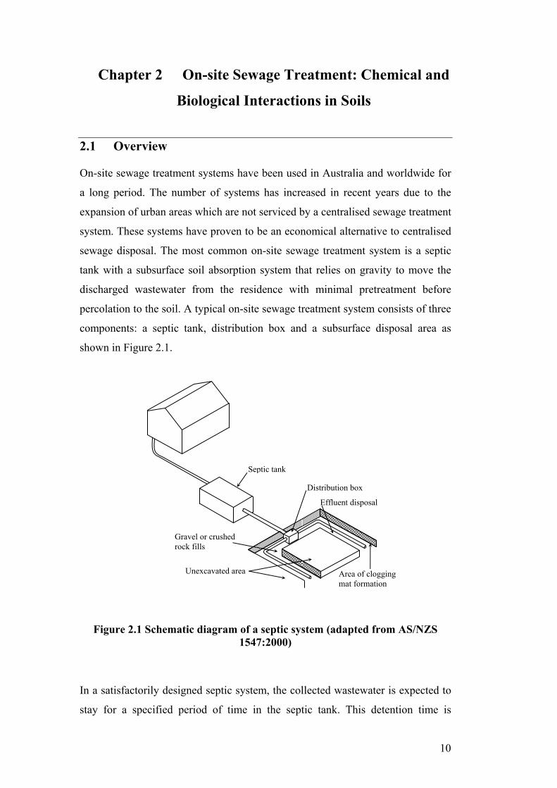
percolation to the soil. A typical on-site sewage treatment system consists of three

components: a septic tank, distribution box and a subsurface disposal area as

shown in Figure 2.1.

Figure 2.1 Schematic diagram of a septic system (adapted from AS/NZS 1547:2000)

In a satisfactorily designed septic system, the collected wastewater is expected to

stay for a specified period of time in the septic tank. This detention time is

Septic tank

Distribution box

Gravel or crushed rock fills

Effluent disposal

Unexcavated area Area of clogging mat formation

11

required to remove most of the settleable solids and floatable greasy material from

the wastewater. The septic tank provides primary treatment for the discharged

wastewater by acting as an anaerobic bioreactor that allows incomplete digestion

of retained organic matter. After that, effluent leaves the septic tank to the

distribution box to be discharged to the subsurface disposal area. The discharged

effluent contains a significant amount of contaminants such as nitrogen,

phosphorus, pathogens and soluble organic matter for advanced treatment by the

soil. However, the discharging of effluent over a poorly structured soil with weak

physical or chemical characteristics can lead to serious environmental

consequences, such as degradation of the soil and pollution of the

surface/groundwater. Therefore, the soil must have a suitable permeability for

effluent transmission and physico-chemical characteristics that enable it to handle

effluent application and remove pollutants before the effluent reaches the surface

and/or groundwater.

2.2 Treatment System Performance

An ideal on-site sewage treatment system is expected to function well if it is

installed properly in an area with suitable soil. The soil is considered suitable if it

has the capacity to percolate the incoming effluent load and provide the necessary

treatment to meet public health, ground and surface water standards, and protect

the environment. The subsurface disposal area is the most critical component of

the on-site sewage treatment system. This area is expected to provide the final

treatment of the discharged effluent.

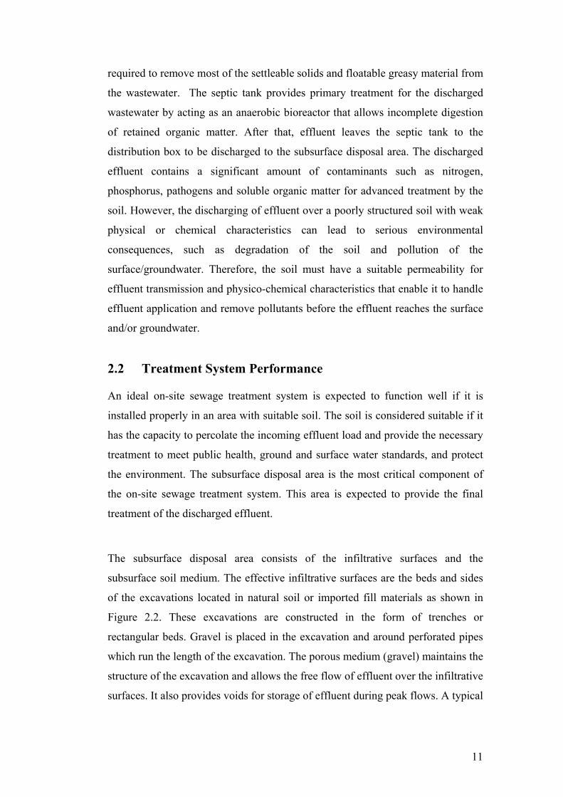
The subsurface disposal area consists of the infiltrative surfaces and the

subsurface soil medium. The effective infiltrative surfaces are the beds and sides

of the excavations located in natural soil or imported fill materials as shown in

Figure 2.2. These excavations are constructed in the form of trenches or

rectangular beds. Gravel is placed in the excavation and around perforated pipes

which run the length of the excavation. The porous medium (gravel) maintains the

structure of the excavation and allows the free flow of effluent over the infiltrative

surfaces. It also provides voids for storage of effluent during peak flows. A typical

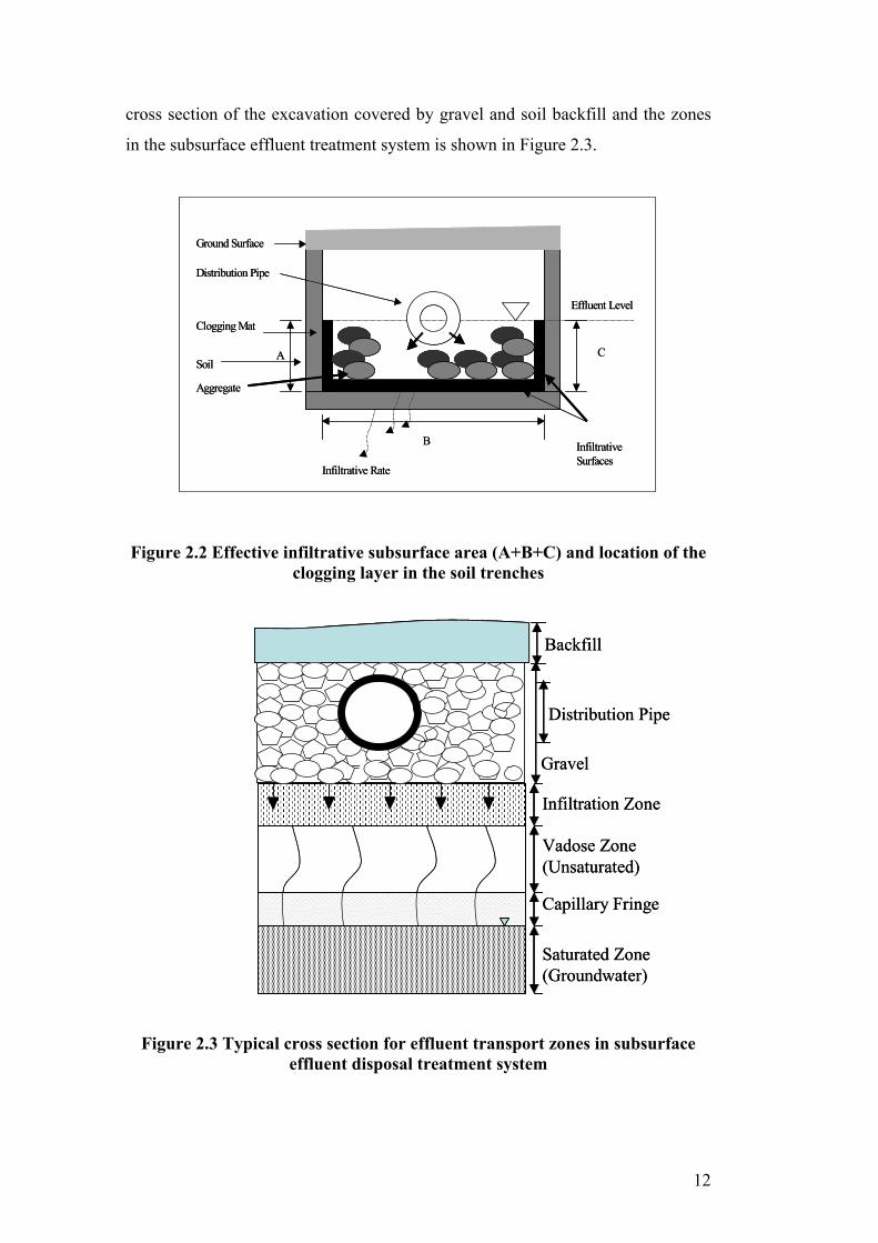
12

cross section of the excavation covered by gravel and soil backfill and the zones

in the subsurface effluent treatment system is shown in Figure 2.3.

Figure 2.2 Effective infiltrative subsurface area (A+B+C) and location of the clogging layer in the soil trenches

Figure 2.3 Typical cross section for effluent transport zones in subsurface effluent disposal treatment system

Backfill

Gravel

Distribution Pipe

Infiltration Zone

Vadose Zone(Unsaturated)

Capillary Fringe

Saturated Zone (Groundwater)

Backfill

Gravel

Distribution Pipe

Infiltration Zone

Vadose Zone(Unsaturated)

Capillary Fringe

Saturated Zone (Groundwater)

Effluent Level

A

B

Infiltrative Rate

Ground Surface

Distribution Pipe

Clogging Mat

Soil

Aggregate

Infiltrative Surfaces

C

Effluent Level

A

B

Infiltrative Rate

Ground Surface

Distribution Pipe

Clogging Mat

Soil

Aggregate


C

Effluent Level

A

B

Infiltrative Rate

Ground Surface

Distribution Pipe

Clogging Mat

Soil

Aggregate


C

13

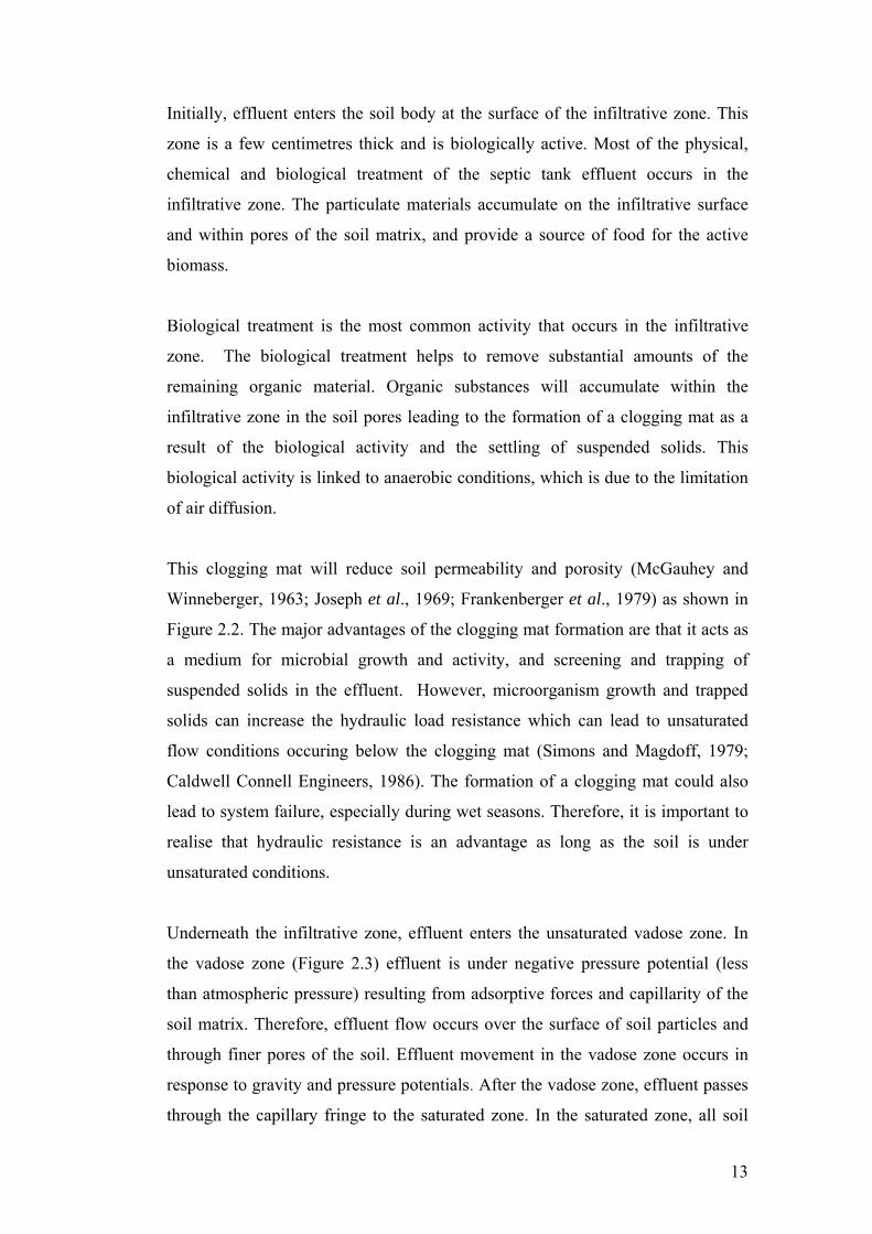
Initially, effluent enters the soil body at the surface of the infiltrative zone. This

zone is a few centimetres thick and is biologically active. Most of the physical,

chemical and biological treatment of the septic tank effluent occurs in the

infiltrative zone. The particulate materials accumulate on the infiltrative surface

and within pores of the soil matrix, and provide a source of food for the active

biomass.

Biological treatment is the most common activity that occurs in the infiltrative

zone. The biological treatment helps to remove substantial amounts of the

remaining organic material. Organic substances will accumulate within the

infiltrative zone in the soil pores leading to the formation of a clogging mat as a

result of the biological activity and the settling of suspended solids. This

biological activity is linked to anaerobic conditions, which is due to the limitation

of air diffusion.

This clogging mat will reduce soil permeability and porosity (McGauhey and

Winneberger, 1963; Joseph et al., 1969; Frankenberger et al., 1979) as shown in

Figure 2.2. The major advantages of the clogging mat formation are that it acts as

a medium for microbial growth and activity, and screening and trapping of

suspended solids in the effluent. However, microorganism growth and trapped

solids can increase the hydraulic load resistance which can lead to unsaturated

flow conditions occuring below the clogging mat (Simons and Magdoff, 1979;

Caldwell Connell Engineers, 1986). The formation of a clogging mat could also

lead to system failure, especially during wet seasons. Therefore, it is important to

realise that hydraulic resistance is an advantage as long as the soil is under

unsaturated conditions.

Underneath the infiltrative zone, effluent enters the unsaturated vadose zone. In

the vadose zone (Figure 2.3) effluent is under negative pressure potential (less

than atmospheric pressure) resulting from adsorptive forces and capillarity of the

soil matrix. Therefore, effluent flow occurs over the surface of soil particles and

through finer pores of the soil. Effluent movement in the vadose zone occurs in

response to gravity and pressure potentials. After the vadose zone, effluent passes

through the capillary fringe to the saturated zone. In the saturated zone, all soil

14

pores are filled with water and the flow occurs under a positive pressure gradient

(Anderson et al., 1988; Robertson et al., 1989).

Successful management of a subsurface effluent disposal system is limited by the

characteristics of the site selected for effluent treatment. Therefore, subsurface

effluent treatment system performance is difficult to predict since each site is

unique.

2.3 Hydraulic Performance The primary requirements for the successful performance of an on-site sewage

treatment system are a satisfactory ability of soil to accept and transmit effluent

(hydraulic conductivity), adequate soil volume and/or depth, and the lack of other

site constraints such as steep slope, flooding, high water table and shallow

bedrock (Bouma et al., 1972). The failure to meet one of those requirements can

lead to serious environmental and public health problems, especially if effluent

pollutants, such as pathogens, phosphorus or nitrogen, reach the water body where

they could potentially be transferred to humans through consumption of water or

food.

The hydraulic performance of a subsurface effluent disposal system is measured

by its ability to accept all the effluent received during its design life. Continuous

effluent application will lead to the formation of the biological layer on the

infiltrative surface. The formation of the thin biological layer will reduce and

change the capacity of an infiltrative system to accept and percolate effluent to

deeper soil layers. The reduction in percolation rate reaches an almost steady state

over time. This flow rate is known as the long-term acceptance rate (LTAR).

The soil acts as a support medium for the clogging mat. The clogging layer will

always form over the interface between the trench and the soil body, but the

LTAR varies between soils (Healy and Laak, 1974). LTAR is high for a sandy

soil due to high permeability and low for clayey soil due to low permeability

(Laak, 1973). The clogging mat will form on the interface berween the trench and

the soil body regardless of the surface condition, orientation and angle

(Winneberger et al., 1962; Kropf, 1975).

15

Excessive clogging at the infiltrative surface will lead to effluent ponding due to

the reduction of the infiltrative rate below the actual application rate. The extra

amount of effluent ponded can cause hydraulic failure in the subsurface effluent

disposal system (Bouma et al., 1974; Kristiansen, 1982; Otis, 1984; Siegrist et al.,

1984).

Hydraulic failure occurs for various reasons such as the decrease in soil

permeability and porosity. The applied effluent can no longer freely enter or

leave the soil pores. The effluent movement through the soil will decrease, which

will restrict the openings or reduce the size of soil pores and thereby reduce soil

permeability. Compaction and smearing of the infiltrative surface during

construction or depositing of suspended solids entering the system with the

effluent can seal the entrances to the pores, which could also lead to hydraulic

failure. The gas released due to the biological activity in the soil or air trapped

below the wetting front can prevent liquid from entering the pores, which could

cause hydraulic failure. Soil swelling from prolonged wetting can close the pores.

Biological activity stimulated by the carbonaceous material and nutrients in the

effluent can degrade the soil structure resulting in the reduction of macropores.

The biomass and metabolic by-products produced by microbial activity can fill or

reduce the size of the pores. All these processes occur to some degree in

subsurface wastewater infiltration systems (Otis, 1984; Kristiansen, 1982).

Therefore, it is important to consider the hydraulic infiltrative failure factor in on-

site sewage treatment system design.

Allison (1947), Jones and Taylor (1965), Thomas et al. (1966), and Okubo and

Matsumoto (1979) investigated the various phases of soil clogging and formation

of the biological clogging mat. Allison (1947) stated that infiltrative rates of

groundwater-recharge basins receiving river water initially decline and then

increase before slowly declining to a small fraction of the initial infiltrative rate.

The initial decline in the first phase was attributed to structural changes in the soil

resulting from swelling and dispersion of dry clay minerals. The steady increase

in the second phase was related to the dissolution of entrapped air in the soil

pores. In the third phase, the rate decreased rapidly at first and later more slowly.

Allison (1947) concluded that biological activity was responsible for the loss in

16

permeability due to clogging, resulting from the production of active biomass and

metabolic by-products such as slimes and polysaccharides.

Jones and Taylor (1965) applied septic tank effluent sporadically to sand columns

and also noticed a three-phase reduction in infiltrative rates, but in a different

way. The daily dosed effluent on the columns resulted in a rate of decline which

was directly proportional to the volume of infiltrated effluent. In the first phase,

the cause of infiltrative rate decline was considered to be a result of the

accumulation of organic solids which proceeded more slowly in the second phase.

This was apparently due to a quasi-equilibrium state, which was reached between

organic matter decomposition and new solids accumulation. The infiltrative rate

declined rapidly during the third phase and stabilised. This decline appeared to be

independent of effluent loading or the initial rate of infiltration. In columns that

were continuously ponded, the second phase was of short duration or absent.

Thomas et al. (1966) sporadically applied septic tank effluent to columns of sand.

They also found three separate phases of hydraulic behaviour, but the way in

which the infiltrative rates declined in response to daily dosing of septic tank

effluent was once again different. In the first phase, the rate of infiltration

declined slowly over an extended period of time. The second phase was short,

during which time the infiltrative rate declined sharply and incessant ponding

occurred. In the third phase, the infiltrative rate reached a very low limit. It was

noted that the change from the first to second phase corresponded with a shift

from an aerobic to an anaerobic soil condition below the infiltrative surface.

Okubo and Matsumoto (1979) reported four phases of soil clogging from their

experiments with the application of synthetic wastewater to columns of sand. The

columns were continuously fed with an artificially prepared wastewater

containing glucose as the only carbon source. Ammonium chloride was added to

produce nitrogen. Other micronutrients were also added. In the first phase,

infiltrative rates decreased rapidly and this was followed by almost constant and

sometimes increasing rates in the second phase. The third phase showed a rapid

rate of decline. In the fourth phase, the infiltrative rate slowly decreased to a

fraction of the initial rate. During the third phase, a change from aerobic to

17

anaerobic conditions was observed in the soil gas. It appears that the reduction in

the infiltrative rate in the first phase was due to the slow build-up of a slimy layer

on the soil surface. The infiltrative rate initially increased in the second phase due

to microbial activity. The decline of the infiltrative rate was due to the change

from an aerobic to anaerobic condition because of effluent ponding. Finally, the

infiltrative rate slowly declined in the fourth phase due to anaerobic microbial

activity.

Differences between the observations of the previous four studies are attributed to

the variations in the methods used to conduct the column experiments and the

type of effluent and the soil type used for the experiment. On the other hand there

are also similarities in their outcomes. In general, a slow decline in the infiltrative

rate was observed during the first phase. Also, in some of the studies a rapid

decline occurred during the overall declining phase. This period of rapid decline

in infiltration is a result of biological and chemical activity within the soil under

the infiltrative surface. These studies concentrated on the phases of clogging mat

formation based on the effluent or water percolation in sand columns. None of the

researchers investigated the formation of clogging on the surface of undisturbed

soil columns to understand the actual soil performance under effluent application.

2.4 Mechanisms of Clogging McCalla (1945, 1950) conducted a series of studies from which he concluded that

microorganisms were the cause of reduced water percolation through soils. One

of these studies used three sets of columns. Each set contained a different soil type

(Sapsburg silty clay loam, Peorian loess and Hisperia sandy loam). One set

received distilled water only, another was covered with cotton gin waste mulch

before distilled water was applied, and the third had mercury chloride added to the

water to act as a disinfectant. The sets were continuously ponded. The results

showed dramatic decreases in the rate of water infiltration in the first two sets, but

the columns to which mercury chloride was added maintained infiltrative rates

near the initial values. McCalla (1950) concluded that micro-organisms caused

the reduced water percolation either by producing gases or organic materials, such

as slimes, which interfere with water movement; or by decomposing or changing

the binding agents responsible for stabilising the soil structure.

18

Allison (1947) conducted classical experiments where clogging occurred in

columns of three sterilised soils, Hanford loam from Neara River, Exeter sand

loams from Kern County and Hesperia sandy loam from Kern County. Half of

the columns were re-inoculated with microorganisms after sterilisation. Sterilised

tap water was ponded continuously over the columns. Only the sterilised columns

receiving the sterilised tap water remained at maximum permeability throughout

the test. Both the control soil and the re-inoculated soil clogged readily. Allison

(1947) concluded that soil clogging is generally explained by microbial activity

and that a certain degree of clogging must always be expected when non-sterile

water is infiltrated into soil.

Gupta and Swartzendruber (1962) reported similar results, which confirmed the

previous results from McCalla (1945, 1950) and Allison (1947), and went on to

show that clogging occurs near the infiltrative surface. In this experiment boiled

deionized water with and without phenol was injected into the bottom of columns

filled with clean testing sand. Piezometers showed within one day that head

losses through the first few centimetres of the columns injected with the phenol-

free water were substantial and increased with time. When phenol was added or

the temperature reduced from 23oC to 1.5oC, little head loss was observed. Also,

the bacterial counts taken from increments throughout the column showed

maximum numbers at the inlet. Gupta and Swartzendruber (1962) concluded that

the cell mass alone could not account for the reduction in the permeability

observed. Therefore, it is necessary to consider the whole soil mass for measuring

the soil permeability. In addition, most of these studies used sand as a medium in

the experiments conducted. This does not reflect the actual situation in the field.

It is important to examine these outcomes on natural soil.

The column studies conducted by Jones and Taylor (1965) and Thomas et al.

(1966) also showed clogging to be primarily a surface phenomenon. Septic tank

effluent was applied to columns of sand in both studies. Jones and Taylor (1965)

placed gravel on the sand surface to replicate a subsurface effluent treatment

system. The experiment showed that a zone of low conductivity developed at or

just below the gravel and sand interface. Incremental analyses with depth for

organic and inorganic materials in the gravel and sand columns revealed two

19

distinct zones of accumulation. The first zone was the gravel and sand interface

region and the second zone was the top few centimetres of the gravel. The lower

ratio of organic to inorganic materials in the gravel as compared to the interface

region suggested that biological degradation was more rapid in the gravel due to

better aeration.

Bliss and Johnson (1952) and Johnson (1957) studied different methods to

maintain high infiltrative rates in soils under prolonged submergence in

percolation ponds used for groundwater replenishment. The infiltrative rates

improved when organic materials were added to the soil, but only after a period of

preliminary decomposition or “incubation” and air-drying. They found that

during the incubation period, the infiltrative rates decreased, but during the

reapplication of water following the drying period, infiltrative rates increased

considerably. Rates once again decreased with time to low levels, at which time

amalgamation of fresh organic materials became necessary. The phenomenon

was described as a three-phase process consisting of an incubation period, post-

drying phase and final infiltrative rate decline (Bliss and Johnson, 1952). During

the first phase or incubation period, microbial activity increased when water with

the incorporated organic matter was applied to the soil. A significant amount of

gums, gases and other by-products were produced which sealed the soil pores. At

this point it was necessary to begin the second phase which is the drying process

of the soil. Without this, no increase in rates followed. During the drying phase,

the microbes and by-products contracted and formed a type of waters table

coating, pulling the soil particles together into aggregates. The results showed

that the soil treated in this manner could provide large increases in total and non-

capillary porosity. The repetition of liquid application enlarged the pores making

them more stable permitting rapid infiltration. Eventually, the binding agents also

decomposed and the aggregates broke down to cause a dramatic decline in

infiltrative rate.

Siegrist (1987) confirmed that the type and amount of wastewater solids applied

to the soil were important factors affecting the rate of clogging. Also, the

observed infiltrative rate response patterns paralleled the previously observed

three-phase soil clogging process. In the study undertaken by Siegrist (1987),

20

gravel-filled, cylindrical, field test-cells constructed in silty clay loam subsoil

were applied with effluent for several years with one of three different domestic

categories of waters: tap water, grey water septic tank effluent, and conventional

septic tank effluent. Undisturbed soil samples and cores were collected from the

sites at selected depths for the purpose of characterising a wide variety of physico-

chemical, morphological, and micro-morphological soil properties. The study

showed that the clogged infiltrative surface zones had elevated water content and

organic matter accumulation at and immediately beneath the soil infiltrative

surface. In all cases, the organic material was found to be concentrated near the

infiltrative surface and was effective in blocking and filling soil pores, thereby

reducing native soil infiltrative rates. Also, all soil sites that experienced clogging

exhibited a variable-length initial period of operation characterised by an

infiltrative rate which gradually declined from near-initial levels. Subsequently,

there was a substantial and steady decline. The long-term infiltrative rate

approached zero as intermittent and then continuous ponding of the soil

infiltrative surface developed and grew as the clogging mat increased in

magnitude.

In general, the mechanisms responsible for soil clogging development were not

clearly evident. However, Siegrist (1987) concluded that soil clogging might

have been caused by processes similar to humus development in native soils.

Humus is known to form in the soil from a wide variety of precursors including

readily degradable organic compounds. Humus develops under specific

conditions, which include cool temperatures, high humidity, and restricted

aeration with an influx of organic materials and nutrients. Discharged effluent to

the subsurface disposal area usually carries different pollutants such as organic

matter and nutrients. The loading rates of these pollutants usually exceed the

formation of humus at the infiltrative surface which usually leads to the failure of

the sub-surface area.

2.5 The Soil as a Treatment Medium Great emphasis has been placed on the soil as a repository for effluent from on-

site wastewater treatment systems. Soil treatment of waste is dependent on

chemical, physical and biological processes retaining and altering contaminants

21

and on transmission of effluent. Since the performance of a soil depends on its

characteristics, reaching a greater understanding of soils and their behaviour under

effluent application was a major component of this research project. The

prediction of soil performance under effluent application is not easy due to its

heterogeneity and complexity. The composition of soil controls effluent

transmission through the different layers. Soil with clayey particles is expected to

slow effluent percolation, while soils with a high percolation rate are expected to

have a coarse texture with less clay content (Bell, 1993). The soil texture is

described as the relative proportions of sand, silt and clay in a soil.

Soil water interaction and the soil’s ability to provide the necessary treatment

mechanisms are necessary for successful transport of the discharged septic tank

effluent to the subsurface layers. The understanding of soil composition and

classification enables the transfer of the soil information from one geographic area

to another, and helps predict the suitability of soils for effluent treatment.

2.5.1 Soil Definition and Composition

Soil is defined as a thin layer of unconsolidated material covering the land surface

of the earth and the medium where most plants grow (Bridges, 1978). Soil is

considered to be a weakly cemented accumulation of mineral particles formed

from weathering of rocks, with the void space between particles containing water

and/or air (Grim, 1968).

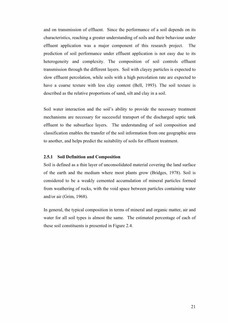
In general, the typical composition in terms of mineral and organic matter, air and

water for all soil types is almost the same. The estimated percentage of each of

these soil constituents is presented in Figure 2.4.

22

Figure 2.4 Approximate percentages of constituents in soils (Bridges, 1978)

The solid phases of the soil are minerals remaining after weathering such as

quartz, and reformed minerals such as clay minerals and/or organic matter

occupying almost 50% of the soil volume in the upper layer but often increasing

to around 60% at the subsurface layers (Bridges, 1978). The organic fraction

includes residue in different stages of decomposition as well as active organisms.

The ratio of air to water in the remaining volume of the soil (pore space) changes

widely from one soil to another based on the soil structure, bulk density snd

texture. The mineral portion consists of particles of varying sizes, shapes and

chemical composition. The main constituents of soil are the mineral elements

(inorganic component), which include all minerals weathered from the parent

material as well as those formed in the soil from substances percolating through

the soil matrix. The inorganic component consists of particles of sand, silt and

clay as presented in Table 2.1.

Table 2.1 Different size fractions of soils (Bridges, 1978)

halla

This figure is not available online. Please consult the hardcopy thesis available from the QUT Library

halla

This table is not available online. Please consult the hardcopy thesis available from the QUT Library

23

A common characteristic of all soils is the presence of organic matter, which is

responsible for the darkening of the surface or upper soil horizon. The organic

matter level declines to its lowest values in the subsoil layers. Organic matter in

soils can have a major impact on the soil properties (Bell, 1993). The

characteristics of the two components are as follows:

• Non-living component - this serves as a reservoir of plant nutrients, such as

nitrogen and phosphorus. In addition, the non-living components are

important in maintaining and developing the soil structure. The soil structure

is the aggregates of soil particles into larger particles or clumps. This

arrangement modifies the bulk density and porosity of the soil. The negative

charge on the non-living colloidal component is important in the retention of

cations and water (Ellis, 1972).

• Living component (or soil organisms) – this is important for fertility by

releasing the nutrients from residues and humus by either the

mineralisation/demineralisation processes, or by the fixation of nitrogen by

Rhizobium bacteria on legume roots (Rowell, 1963).

Soil organic matter content influences the degree of aggregation and aggregate

stability (Mbagwe and Piccolo, 1990) and it can reduce the bulk density and

increase total porosity and hydraulic conductivity in heavy clay soils (Anikwe,

2000). The remaining portion of the soil volume is occupied by air and water,

which fill the pores in the soil. Soil air is similar in composition to the atmosphere

above the soil, but in the case of a saturated soil, water drives out most of the air.

Organic matter is considered a major component of soil composition; its content

plays a major role in the effluent renovation process (Mitchell, 1932; Thomas and

Bendixen, 1969; Hamaker, 1972). The uptake and fixation of nitrogen are

important mechanisms for the handling and renovation of effluent contaminants

by the soil. Organic matter has a certain capacity for holding nutrients under

continuous effluent application. Due to this limited capacity, the role of clay

minerals will have a significant impact on effluent renovation because of the

presence of electrical charges available on the clay particle surface and the

potential for cation exchange.

24

2.5.2 Mineralogy of the Clay Fraction

Clay minerals play a key role in determining the transport of effluent

contaminants through the soils (Bear, 1965; Tan, 1992; Waddell and Weil, 1996;

Khalil et al., 2003). A large variety of minerals with varying degrees of

crystalinity occur in the clay fraction of soils. These clay minerals offer three

advantages. Firstly, they have a large specific surface area (between 10 and 700

m2/g) in comparison to other solid phase components (Fripiat, 1965; Johnston,

1996). The specific surface area of a soil is the ratio of surface area to volume,

which is measured as the surface area per unit mass, assuming a constant particle

density. Secondly, this large surface area is often associated with electrical

charges. This electrical charge is due to isomorphic substitution, defects and

broken edges in clay mineral crystal structures (Johnston, 1996). These charges

result in accumulation of inorganic and organic cations and are responsible for the

high water retention capacity of many types of clays (Barriuso et al., 1994; Farrell

and Reinhard, 1994). Finally, naturally occurring clay mineral particles can be

coated by amorphous oxide hydroxides and humic materials and thus serve as

efficient templates for secondary solid phases (Johnston, 1996). Due to these

advantages, the clay minerals are considered very important in the chemical and

physical reactions involved in effluent renovation (Fripiat, 1965; McBride et al.,

1977; Brady and Weil, 2002).

The soil adsorption capacity is associated with electrical charges available at the

surface of the clay particles. Some of the clay particles have a permanent

negative charge that holds exchangeable cations close to the particle surface and

in their interlayer. Other clay minerals have a charge that varies with pH,

resulting in charges that will be negative at a high pH and positive at a low pH

(Helling, 1964; Johnston, 1996). The functional surface charge capacity (τ) of the

clays can be calculated based on the ratio of cation exchange capacity

(CEC)/specific surface area (Table 2.2). The values of τ are quite similar for the

different clay minerals, which means that the clay crystals cannot obtain an

indefinite number of negative charges and remain stable. On the other hand, for

minerals bearing predominantly pH dependent charges, both the CEC and anion

exchange capacity (AEC) can be significant, depending on the prevailing pH.

Therefore, the adsorption of effluent pollutants by clay particles depends not only

25

on their large specific surface area but also on the nature of the clay minerals

present in the soil. In addition, the pH level controls the type of charges available

for adsorption mechanisms and also desorption if the pH changes.

Table 2.2 Cation exchange capacities and surface charge densities for some of

the clay minerals as reported by White (1997)

The basic structural units of most clay minerals consist of sheets of silicon

tetrahedra and aluminum octahedra. Silicon, magnesium, iron and aluminum may

be partially replaced by other elements in these units by a process known as

isomorphous substitution (Sposito, 1984; Norris et al., 1992; Mitchell, 1993;

Johnston, 1996). Isomorphous substitution is of vital importance because it is a

primary source of both negative and positive charges on clay minerals (McNabb,

1979; Johnston, 1996). The basic clay sheets combine either in a 1:1 or 2:1 ratio

to form the clay minerals such as kaolinite, illite and montmorillonite.

The importance of kaolinite is due to its structural arrangement. The kaolinite

structure is based on a single sheet of silicon tetrahedra (Figure 2.5) combined

with a single sheet of aluminum octahedra (Figure 2.6). These two sheets are

bonded through shared oxygen atoms to form a layer. The kaolinite particle

consists of repetitions of these layers bonded by hydrogen ions (stacking) (Bear,

1965; Schrader and Yariv, 1990; Norris et al., 1992). Because of the kaolinite

structure, the siloxane and gibbsite-lite sheets are exposed and can interact with

the different components in the soil (Grim, 1968; Allen and Hajek, 1989; Bish and

Guthrie, 1994). Due to kaolinite’s well-packed structure, it is difficult to break

down and the kaolinite layers are not easily separated (Figure 2.7). Most of the

sorption activity occurs in the kaolinite along the edges and outside surfaces.

Kaolinite could form a barrier that is not easily degraded and naturally occurring

sediments and deposits containing an abundance of kaolinite interspersed with

halla


26

other minerals are effective in controlling the migration of dissolved matter

(Devidal et al., 1996). Therefore, the soils with large quantities of kaolinite are

expected to have a low percolation rate due to the compact structure. Kaolinite

exhibits less plasticity, stickiness, cohesion, shrinking and swelling and can hold

less water than other clays. Due to these properties, kaolinite is used for

cultivation, and with proper nutrient management can be quite productive (Brady

and Weil, 2002). Kaolinite is considered one of the most abundant minerals in

soils and sediment. Its properties are such that it interacts with other soil elements

to contribute to soil stability (Huertas et al., 1999).

Kaolinite is considered the least active clay compared to other types of clay (Bish

and Guthrie, 1994; Johnston, 1996; Suraj et al., 1998). Kaolinite has a low CEC

level and the change silanol on the edges and hydroxyls on gibbsite-lite layers is

pH dependent. Therefore, soils with dominant kaolinite content can be expected

to have a limited effluent renovation capacity due to limited charges available for

cation exchange. In Table 2.2, kaolinite is shown as having the least CEC of the

soil minerals.

Oxygen

Si

Oxygen

Oxygen

Oxygen

Oxygen

Si

Oxygen

Oxygen

Oxygen

Figure 2.5 Silicon tetrahedron

OH

OH

OH

OH

OH

OH

Al

OH

OH

OH

OH

OH

OH

Al

Figure 2.6 Aluminium octahedron

27

The illite structure is based on layers consisting of an octahedral sheet of alumina

sandwiched between two tetrahederal sheets of silica. In the octahedral sheet,

there is a partial substitution by Mg2+ and Fe3+ and in the tetrahedral sheet there is

a partial substitution of silicon (Si4+) by aluminum (Al3+). The layers are held

together by a weak bonding through the mica potassium present in the interlayer

(Figure 2.7) (Grim, 1968). Due to the non-expansive nature, the fine-grained

illites are more like kaolinite than smectite with regard to their capacity to absorb

water and cations and their degree of plasticity and thickness (McNabb, 1979).

Figure 2.7 Schematic diagrams: A) kaolinite (1:1) clay structure, B) illite (2:1) clay structure and C) the expanding clay smectite (2:1)

Soils that contain illite in their composition are expected to attract more positively

charged contaminants from the discharged on-site effluent than kaolinite due to

the higher surface charge of illite. The contaminants are of a form that they can be

easily remened/detained by the CEC such as Na+.

Smectites form a special group in the phyllosilicates or layer silicates. Smectites

are characterised by a 2:1 layer structure similer to illite in which two tetrahedral

sheets form on either side of an octahedral sheet through sharing of apical oxygen.

As the apical oxygen from the tetrahedral sheet form ditrigonal or hexagonal

rings, one-oxygen ion from the octahedral sheet is located in the centre of each

ring and is protonated to yield a structural hydroxyl group (Kloprogge et al.,

1999). The smectite structure is almost the same as that of illite, but in the

octahedral sheet, there is possible partial substitution of aluminum by Mg2+, Fe2+

or Fe3+ and Al-Si substitution in the tetrahedra sheet is also possible. K+ can also

28

be present in smectite but hydrated, which is not the case in illite. Water

molecules and exchangeable cations other than potassium may occupy the space

between the layers, and due to these ions, there is a weak bond between the layers.

Considerable swelling of smectite may occur due to additional water being

adsorbed between the layers and then shrinking when the water is removed.

Hence these high shrink/ high swell soils have an ability to reset the structure

units (Call, 1957; Grim, 1968; Johnston, 1996; Sawhney, 1996). Smectites have a

high amount of mostly negative charges resulting from isomorphous substitution.

Most of the charges come from Mg2+ ions substitution with Al3+ positions on the

octahedral sheet such as montmorillonite, nontronite and hectorite minerals. In

addition, some charges are derived from substitution in the Al3+ ions for Si4+ in

the tetrahedral sheet such as beidellite and saponite minerals. Because of these

substitutions, the cation exchange capacity is very high; around 20 to 40 times the

CEC of kaolinite depending on the smectite group involved as shown in Table 2.2

(Reid and Ulery, 1998). Smectite clays can be expected to provide a higher

renovation capacity for applied effluent than kaolinite and illite, due to the amount

of charges available for the cation exchange process.

2.5.3 Soil Profiles

Soils are characterised by the formation of a profile consisting of several horizons

parallel to the surface layer. These horizons are the surface, the subsoil and the

decomposing parent material horizons which are named A, B and C respectively.

Also, soil horizons can be divided into sub-horizons. The soil layers differ from

the layers above or below in one or more soil properties such as thickness, colour,

texture, structure, consistency and the chemical composition. In some cases,

boundaries between different horizons merge gradually over several centimetres

and are difficult to observe without close examination (Bridges, 1978).

Bridges (1978) reported the following definitions for the different soil horizons:

• A-horizon (surface soil) is the zone of most biological activity. The

surface soil layer is usually dark, resulting from an accumulation of organic

matter over time and is the zone of maximum eleviation or leaching

involving weathering of minerals and transport of clay sized material to the

29

subsoil (B-horizon). The A-horizon can be subdivided into two sections:

A1-horizon with a thickness of 50 to 300 mm, which is generally dark as a

result of the high organic matter content; and A2-horizon is a paler in colour

which comes underneath A1-horison with 50 to 500 mm or more in

thickness.

• B-horizon is the subsoil layer, which may vary in depth from 100 mm to in

excess of 2 m. The B-horizon is characterised by lower biological activity

lower levels of organic matter, higher content of clay minerals, iron and

aluminium oxyhydroxides, and higher bulk density than the A-horizon.

Also, the structure of the subsoil layer is more compacted than the surface

layer with red and yellow colours resulting from the accumulation of iron

compounds. The B-horizon has lower levels of available nutrients, higher

levels of soluble salts and poorer drainage than the A-horizon. The B-

horizon can be divided into two sections based on the soil structure, the

change in the soil structure from unconsolidated to bulky or the other way

around. The upper section is the B1-horizon and when there is a change in

colour or structure, the underlying section is considered as the B2-horizon.

• C-horizon includes the weathered, consolidated or unconsolidated layers of

parent material below the B-horizon, which are unchanged by biological

soil-forming processes. The C-horizon is recognised by its lack of

pedological development, and by the presence of remans of geological

organisation. Its thickness is very variable.

2.5.4 Soil Classification

Soil classification is a basic requirement for organising the knowledge of different

soil types and their properties. Soils are three-dimensional bodies and their

classification has always caused problems for scientists and those who use the

land. These problems occur due to the wide range of parent materials and the

different levels of soil weathering in various parts of the world. Soils contain a

diversity of colloidal particles including clay minerals and organic matter.

Soil classification is not consistent all over the world, with each country trying to

develop a special classification according to criteria available in that country.

30

Therefore, soil classification is still under development. However, there have

been attempts to develop a soil classification based on a comparison of mature

soils with endeavours at grouping in logical and natural system categories.

Different factors affect the soil classification such as change of climate,

cultivation, clearance of vegetation, lowering of groundwater and removal of

salts. Robinson (1947) produced a classification of world soils, which reflected

the approach of pedologists at that time (Table 2.3).

Table 2.3 Classifications of World Soils by Robinson (1947)

The problem with most soil classifications is that they are produced for semi-

natural and natural soils, where in fact, most landscapes have been affected by the

work of humans (Isbell, 1996). There are some soil properties that do not change

materially with agricultural use, of which the texture is the most readily observed

halla


31

feature. Therefore, a classification can be built up quite objectively on soils with

uniform textures (U), soils with textures that gradually change from the surface to

the parent material (G), or soils which abruptly change in texture somewhere in

the soil profile (D). This system has been the basis of the classification map of

Australian soils by Northcote (1960).

Several researchers have developed soil classification systems for Australia.

Stace et al. (1968) classified soils into 19 great soil groups. Also, Northcote

(1979) developed 'A Factual Key' system for the recognition of Australian soils

and this system is used as a basis for the “Atlas of Australia”. Other researchers

such as Beckmann et al. (1987) assembled Australian soils into five broad groups

in an attempt to make it easier for others to use.

The classifications of soil adopted for this research were based on the Australian

Soil Classification developed by Isbell (1996) and Jacquier et al. (2000).

Australia has a great diversity of soils, most of which are ancient, strongly

weathered and infertile. The rest of the soils are young and more fertile. The

Australian Soil Classification, as developed by Isbell (1996) and Jacquier et al.

(2000) considers 14 groups of soil (Table 2.4).

32

Table 2.4 Australian Soil Classification (Isbell, 1996; Jacquier et al., 2000)

Soil Order Suborder Properties Anthroposols

Cumulic, Hortic, Garbic, Urbic, Dredgic, Scalpic and Spolic Anthroposol

Resulting from human activity.

Calcarosols Hypocalcic, Supracalcic, Hypercalcic, Lithocalcic, Hypergypsic, Shelly and Calcic Calcarosol

High calcium carbonate content, shallow depth, and low water retention, high salinity, sodicity and alkalinity.

Chromosols

Red, Brown, Yellow, Black and Grey Chromosol

Clay content increases down the soil profile.

Dermosols

Red, Brown, Yellow, Grey and Black Dermosol

Strongly acidic in high rainfall areas or highly alkaline if it contains calcium carbonate.

Ferrosols Red, Brown, Yellow, Grey and Black Ferrosol

A high free iron and clay content, which can lack strong textural contrast between A and B-horizons.

Hydrosols Supratidal, Extratidal, Hypersalic, Salic, Redoxic and Oxyaquic Hydrosol

Include seasonally or permanently wet soils and the potential drainage of acid sulphate. Hydrosols can create environmental problems such as acidification.

Kandosols

Red, Brown, Grey and Black and Yellow Kandosol.

Mostly well drained, permeable soils.

Kurosols Red, Yellow, Brown, Black and Grey Kurosol

Strongly acid soils with an abrupt increase in clay.

Organosols

Fibric, Hemic and Sapric Organosol

Organic materials control this group by almost 75% of the volume.

Podosols

Aeric, Semiaquic and Aquic Podosol

Controlled by organic matter and aluminium, with or without iron. Low fertility, poor water retention and seasonal waterlogging.

Rudosols

Hypergypsic, hypersalic, Shelly, Carbic, Arenic, Stratic, Leptic, Clastic and Leptic Rudosol.

Have minimal soil development due to their properties or occurrence in arid region.

Sodosols

Red, Brown, Yellow, Grey and Black

Has abrupt clay which increases down the soil profile and high sodium content, which may lead to soil dispersion and instability.

Tenosols

Chernic, Bleached-Orthic, Orthic, Chernic-Leptic, Leptic and Bleached-Leptic

Poor water retention, almost universal low fertility.

Vertosols Aquic, Red, Brown, Yellow, Grey and Black Vertosol

High smectite clay content causing the soil to shrink and crack as the soil dries, and swell when wet.

33

2.5.5 Chemical Reactions

Chemical processes involving soil clay minerals must be taken into consideration

for assessing the suitability of a soil for different purposes, such as sewage

effluent disposal and agricultural use. Therefore, it is essential to have an in-

depth understanding of the chemical processes that occur to enable decisions to be

taken to assess site suitability for effluent renovation purpose.

The chemical processes in soil have an impact on the concentration of ions and

molecules in soil solutions. The soil solution can be considered to be in quasi-

equilibrium with the solid phase, and the processes of solubilization/precipitation,

ion exchange, absorption/desorption and mineralization/ immobilization can alter

its composition (Bell, 1993).

Wiklander (1964) defined ion exchange as the reversible process by which cations

and anions are exchanged between solid and liquid phases and between solid

phases if in close contact with each other. Cation exchange processes are

considered to be the dominant process in soils for the removal pollutants from the

applied effluent. Ion exchange is governed mainly by electrostatic bonding and is

influenced by the valency and hydration of the ion involved and the location and

density of the charge on the solid component of the soil (Ellis, 1972).

Chemical bonding may occur in several forms between ions and the solid phase of

the soil during the process of ion exchange. The chemical bonding ranges from

electrostatic to covalent, the bonding between ions and the solid phase is more

covalent. The bonding process is generally limited for the ion involved and not

interchangeable to other ions of the same charge. Accordingly, this type of

bonding is not strictly exchangeable, and is considered as an adsorption reaction.

The interaction of organic solutes with the clay surface is based on the chemical

and physical properties of the surface which contribute to the clay activity. The

emphasis is not on the bulk mineralogy or structures of the various clay minerals,

but rather on the active surface characteristics associated with these clays.

However, understanding the surface structure and reactivity of clay minerals is

34

often a direct consequence of the clay minerals’ bulk structure (Bailey, 1984;

Brindley and Brown, 1980; Bailey, 1988; Bish and Guthrie, 1994)

In general, there are six predominant active surface sites on the clay minerals.

1. Natural siloxane surface. These surfaces occur on 1:1 and 2:1 layer

silicates where no isomorphic substitution takes place such as talc and

pyrophyllite. These clay surfaces function as a weak Lewis base i.e.

electron donor (Jensen, 1978). Also, they have very low affinity for water

(Schrader and Yariv, 1990; Norris et al., 1992). As a result, the siloxane

surface is found to be rather inert and unreactive due to the strong bonding

between Si and O atoms.

2. Isomorphic substitution surface. These clay surfaces are characterised

by permanent negative charges, which occur in the clay lattice of 2:1 layer

silicates such as smectite, vermiculites and micas. Isomorphic substitution

occurs in either the octahedral or tetrahedral sheet. Clays vary in the

degree of substitution (Johnston, 1996). Also, the location of isomorphic

substitution in the 2:1 layer silicates has a large influence on the sorption

capacity of polar and charged organic solutes (Johnston, 1996). Finally,

the degree of swelling and accessibility of the interlayer region are

strongly influenced by isomorphic substitutions.

3. Metal cations occupying cation exchange sites. These sites are directly

related to the sites of isomorphic substitution. In this case, the organic

solutes do not replace the metal cations, but they coordinate directly to the

metal cation (Johnston, 1996).

4. Water molecules surrounding exchangeable cations. This results from

the polarisation of water molecules near exchangeable cations or under

coordinated metal cations at the broken edges.

5. Hydrophobic surfaces. Sorption of organic molecules on clay surfaces

can provide a hydrophobic nature to the clay surface. Smectite surfaces

have a high selectivity for organic cations such as

hexadecyltrimethylammonium (HDTMA) cations (Johnston, 1996).

6. Broken Edges. Hydroxyl groups, such as surface silanol group formed on

the edges of clay minerals. These hydroxyl groups are among the most

35

abundant and reactive sites found on clay particles in the soil and other

subsurface environments (Sposito, 1984).

These six active surface types together with the humic substances are responsible

for the development of pH dependent and independent charges in soils and

sediments. Sites with low pH values develop a positive charge due to the

adsorption of protons. The organic acids (such as formic acid and methanoic

acid) and oxyanions (such as chlorate and chlorite) interact strongly with these

positively charged sites. The increase of pH results in a change to neutral charge

and ultimately to a negative charge when the pH values are greater than the point

of zero charge on the mineral surface. The contribution of the broken edge

surfaces to the CEC depends strongly on the size and shape of the clay particles.

For clays with low or absent isomorphic substitution such as kaolinite, the pH

dependent sites form the main source of reactivity (Bell, 1993; Johnston, 1996).

The pH dependent sorption behaviour of these clay minerals is similar to that of

Fe, Mn and Al hydroxides.

2.5.6 Interaction of Water with Soils

Water is an essential component for every living organism. Water is a simple

chemical compound and has unique properties that promote a wide variety of

physical, chemical and biological processes. In general, soil - water interactions

influence many of the ecological functions of soils and practices of soil

management. Management practices should encourage movement of water into

well-drained soils and maximise the evaporative process (Brady and Weil, 2002).

The influence of the layer charge of the clay mineral that swells with water

extends only a few layers from the surface of the soil with the water forming a

coordination shell around the exchangeable cations. Swelling clay minerals can

keep the water in the interlayer as single, double or triple layers. The water in the

interlayer space of expandable clay minerals is controlled by three factors. They

are firstly, the polar nature of water molecules; secondly, size and charge of

cations; and thirdly, the amount and the location of the charge on the silicate

layers (Reid, 1998; White, 1997; Brady and Weil, 2002; Craig, 1997).

36

In general, charged surfaces of clay minerals are considered to be hydrophilic or

polar in nature due to the presence of a layer of silicate oxygen atoms on the

surface, which can absorb water via hydrogen bonding (Low, 1961). This

excludes kaolinite and siloxane because they are hydrophobic. Sorption of

organics by soils and sediments is reduced in the presence of water (Call, 1957;

Chiou and Shoup, 1985; Ong and Lion, 1991; Pennell et al., 1992; Thibaud et al.,

1993). Call (1957) reported that there is an increase in the adsorption of the

ethylene dibromide (EDB) at low relative humidities of 5, 10 and 20%. This

increase is due to the expansion of montmorillonite interlayer where the EDB can

enter and compete with the water molecules. On the other hand, under dry

conditions, the interlayer remains collapsed and the sorption sites are unavailable.

However, the layer expansion on hydration may allow organics to be sorbed on

the interlayer sites and the extended surface.

The CEC usually quantifies the soil’s ability to exchange cations and to retain

nutrients, reflecting the soil quality (Bear, 1965). The soil’s CEC influences the

interaction of plants with nutrients and contaminants (Tan, 1982). Therefore, the

soil mineralogy and organic matter content are the essential players in the

exchange and absorption processes in the different soil types. Soils with kaolinite

content will provide limited possibilities for cation exchange. Smectite has a

higher CEC than other clays (Table 2.2). Also, as a result of the smectites’

swellability, a barrier layer can be formed. This layer is a disadvantage, as it will

slow down the transport of effluent. However, this layer may also prevent the

contaminants from reaching the groundwater.

2.6 Transport of Effluent Pollutants in Soil and Groundwater Discharged effluent from a septic tank to the subsurface effluent disposal area can

carry various contaminants, such as solids, organic matter, nitrogen, phosphorus

and pathogenic bacteria. A successful on-site sewage treatment system is one

which has the ability to remove the pollutants before the effluent reaches a

surface/groundwater body. During treatment, the septic tank unit will remove

some of the contaminants carried by the effluent. The remainder are discharged to

the subsurface area where the soil is responsible for the treatment activity, acting

as a tertiary treatment system for the discharged effluent. The treatment activity is

37

based on biological and physico-chemical reactions naturally occurring in the soil.

The level of treatment provided is controlled by several factors, such as, effluent

load, bacteria, nutrients and soil physico-chemical characteristics, water table

level, hydraulic loading rate and topography.

Each pollutant requires a certain set of specific removal mechanisms. For

example, solids can be removed by settling or decomposition, but nitrogen

requires various mechanisms, such as nitrification/denitrification, ammonia

fixation, volatilisation and cation/anion exchange processes. Every mechanism

requires certain conditions to occur, which will be discussed in detail in the

following sections.

2.6.1 Solids (Suspended Solids and Dissolved Solids)

The discharged effluent to the subsurface disposal area carries two forms of

solids: suspended solids and dissolved solids. Suspended solids are mostly

filtered by the soil particles in the first few centimetres from the soil surface of the

excavated trenches. The suspended solids are trapped in the infiltrative surface

area due to their large size when compared to the soil’s pore size. Some of the

dissolved solids are consumed by the microorganisms as a source of food

(energy), and the leftovers from the dissolved solids are carried by the effluent

and percolated down through the soil profile. The percolated dissolved solids are

a necessary source of energy for other bacteriological reactions. Therefore, most

of the discharged solids to the subsurface disposal area are removed and handled

within the infiltrative surface area or consumed by bacteria prior to reaching the

surface/groundwater body.

2.6.2 Nutrients (Nitrogen and Phosphorus)

The nutrient concentration contained in effluent is influenced by the use, the type

of human activity and the on-site sewage system operation and maintenance.

Several studies have been conducted over past decades on nutrients discharged to

the subsurface disposal area and the effect of the discharging nutrients on the soil,

and surface/groundwater. Some of these studies discussed the primary factors

associated with the movement and removal of nutrients in soil, such as soil

structure, water table level, dissolved oxygen, organic matter content and

38

exchangeable cation level in the soil (Cochet, et al., 1990; Sawhney, 1996). The

influence of these factors on nutrient movement in soil is significant. Weiskel and

Howes (1992) and Robertson et al. (1998) have reported that data collected from

monitoring wells showed that nutrient concentrations in the effluent decreased

with distance from the effluent disposal area. Walker et al. (1973a) indicated that

the highest nitrogen concentrations could be expected in wells that were a short

distance down the gradient from the effluent disposal system, and the dilution by

the groundwater flow resulted in decreasing nitrogen concentrations further away

from the disposal system. Also, they reported lower nitrogen concentration, as

expected, in wells constructed in the upper gradient region.

Other researchers have studied and monitored nitrogen (N) removal from on-site

wastewater systems and reported that nitrogen could be absorbed into the soil

particles, diluted into the groundwater, or transformed by denitrification as the

main pathways of nitrogen removal (Hinson et al., 1994; Gerrits et al., 1995). It

has been reported that some nitrification takes place in soil layers that are nearly

saturated. On the other hand, Anderson et al. (1998) noted that a considerable

amount of nitrate (NO3-) was transported away from the effluent disposal area of

an on-site sewage treatment system, which was located in an unsaturated soil

containing low organic matter content. However, the movement of NO3- over

long distances towards surface water decreased when the plume encountered

sediments with high organic matter content which indicates that the organic

matter can play a major role in NO3- removal from effluent.

Reneau et al. (1989), Robertson et al. (1989), Weiskel and Howes (1992),

Wilhelm et al. (1994) monitored phosphorus (P) removal from on-site sewage

treatment systems and reported high P removal within short distances from the

infiltration area. Also, the studies reported that the main pathway for P removal

was its precipitation with aluminium (Al3+), iron (Fe3+) and calcium (Ca2+) with

different forms of phosphorus as discussed later in Section 2.6.2B. The

phosphorus discharged from on-site systems is low and the main removal pathway

is precipitation. In addition, the phosphorus precipitation is enhanced by the soil

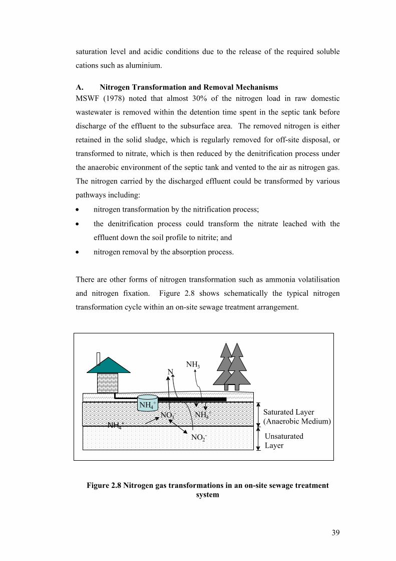
39

saturation level and acidic conditions due to the release of the required soluble

cations such as aluminium.

A. Nitrogen Transformation and Removal Mechanisms MSWF (1978) noted that almost 30% of the nitrogen load in raw domestic

wastewater is removed within the detention time spent in the septic tank before

discharge of the effluent to the subsurface area. The removed nitrogen is either

retained in the solid sludge, which is regularly removed for off-site disposal, or

transformed to nitrate, which is then reduced by the denitrification process under

the anaerobic environment of the septic tank and vented to the air as nitrogen gas.

The nitrogen carried by the discharged effluent could be transformed by various

pathways including:

• nitrogen transformation by the nitrification process;

• the denitrification process could transform the nitrate leached with the

effluent down the soil profile to nitrite; and

• nitrogen removal by the absorption process.

There are other forms of nitrogen transformation such as ammonia volatilisation

and nitrogen fixation. Figure 2.8 shows schematically the typical nitrogen

transformation cycle within an on-site sewage treatment arrangement.

Figure 2.8 Nitrogen gas transformations in an on-site sewage treatment system

NO3-

NH 4 +

NH3

NH4+

N

NH4+

NO2-

Saturated Layer (Anaerobic Medium)

Unsaturated Layer

NO3-

NH 4 +

NH3

NH4+

N

NH4+

NO2-

Saturated Layer (Anaerobic Medium)

Unsaturated Layer

40

Nitrogen primarily exists in the form of ammonium cations (NH4+) within the

discharged effluent leaving the septic tank. Figure 2.8 illustrates the processes for

NH4+ transformation after leaving the tank. The discharged effluent runs through

the trenches and then infiltrates into the soil. About 75-97% of the total nitrogen

contained in the discharged effluent leaves the septic tank in the form of dissolved

NH4+(Walker et al., 1973a,b; Viraraghavan and Warnock, 1975; Stewart and

Reneau, 1981; Robertson et al., 1991; Gerrits et al., 1995).

Robertson et al. (1991) and Weiskel and Howes (1992) reported that the fate of

NH4+ in the soil mostly depends on the water table level. They have recommended

that for on-site effluent disposal systems, the distance between the highest

watertable level and the bottom of the subsurface absorption trenches in the soil

should be kept at least 1 m apart in suitable soil types in order to provide the

required effluent treatment. These suitable soil types for on-site effluent disposal

treatment systems are well-drained soils capable of providing the required effluent

treatment before effluent enters the watertable. In general, soils involved in

effluent renovation perform better if located in areas that do not exhibit a high

watertable, which increases the chances for nitrification processes to occur. As

effluent that contains NH4+ is applied to soils, the oxygen present in the soil pores

facilitates the transformation of NH4+ into NO3

-. In cases where the soil pores are

filled with water (saturated), the amount of oxygen will be reduced and therefore

the nitrification process will decrease. The remaining amount of the nitrogen will

leach with the effluent down the soil profile for further treatment.

The nitrification process requires two steps to be completed. The first step,

undertaken by autotrophic (Nitrosomonas) bacteria, requires a sufficiently high

oxygen concentration in the soil pores to complete the reaction from ammonium

to nitrite. The second step, which is undertaken by the heterotrophic bacteria

(Nitrobacter), quickly transforms nitrite to nitrate.

Autotrophic (Nitrosomonas):

2NH4+ + 3O2 2NO2

- + 4H++ 2H2O

41

Heterotrophic bacteria (Nitrobacter):

2NO2- + O2 2NO3

-

Weiskel and Howes (1992) investigated the level of ammonification in a sandy

soil. They monitored 524 on-site wastewater treatment systems in a 53 ha

residential area in the Indian Heights subbasin located adjacent to Buttermilk Bay,

Massachusetts, USA. The effluent disposal area for these systems was a sandy soil

with less than 1% clay content. Usually, the clay particles carry higher bonding

charges capable of attracting pollutants. In addition, the nitrogen concentration in

the soils in the area was reported as negligible. The study investigated and

documented the depth and surface extension of the plume of contaminants as it

flowed away from the effluent disposal area into the Bay. Weiskel and Howes

(1992) reported that 73% of the dissolved inorganic nitrogen was NO3- in the

plume before reaching the groundwater. The NH4+ in the sandy soil did not fully

transform to NH3 in the monitored area, which means that the NH4+ carried by the

effluent was transformed to nitrate or bonded to CEC of organic residues. This

was due to nitrogen uptake by the organic matter in the soil. The nitrate form of

nitrogen can create serious health problems such as the blue baby syndrome

(methaemoglobinaemia) and environmental problems if it is not absorbed by soil

particles before reaching the water body.

Robertson et al. (1991) monitored two individual households with on-site

wastewater treatment systems situated in sandy soils near Cambridge, Ontario

(Canada). They established a monitoring network of wells in order to document

the depth, width and length of the plume as it flowed away from the effluent

disposal area. The study reported that 100% of the NH4+ was converted into NO3

-

in one site and 67% in the other site. The studies by Weiskel and Howes (1992)

and Robertson et al. (1991) showed that the transformation of NH4+ into NO3

- in

both studies was not always completed.

In the absence of nitrifying/denitrifying bacteria, the nitrification/denitrifying

process will not happen. In such situations, NH4+ can absorb onto soil particles

through adsorption and cation exchange. This process occurs due to the negative

charges available in the soil organic matter and clay particles. The NH4+ adsorbed

42

onto the soil particles can be significant if the level of CEC available for the

absorption is high. In addition, the level and type of other contaminants carried by

the discharged effluent control the NH4+ absorption level by the soil. The absorbed

NH4+ can be nitrified in the future if the soil nitrification conditions improve

(Bicki et al., 1984).

Cogger and Carlile (1984) studied sites located in Craven, Hyde and New

Hanover counties in the lower Coastal Plain of North Carolina, USA. The sites

studied involved septic tanks built on seasonally and continuously flooded soils.

The soil types in the different sites exhibited coarse, silty, fine and organic

textures. The sites with continuously saturated systems recorded high

concentrations of NH4+ and low concentrations of NO3

-, which means that the

ammonium was adsorbed by the soil particles under saturated conditions due to

insufficient oxygen being available in the soil to convert the NH4+ to NO3

-. Carlile

et al. (1981) reported that concentrations of NH4+ and NO3

- decreased with

distance from the effluent disposal area for both continuously flooded and

seasonally saturated systems. In conclusion, the studies suggested that

continuously saturated systems experience little nitrification, which means the

nitrification process declines if the soil reaches the saturation level as a result of

filling the soil pores with water instead of oxygen. Consequently, other

mechanisms such as adsorption or denitrification are more favoured to take place

and denitrification requires reducing conditions (anaerobic/anoxic).

Other types of nitrogen removal pathways are ammonia volatilisation, which is

the conversion of NH4+ into ammonia gas (NH3), uptake of NH4

+ and NO3-, plant

roots and microorganisms (Rowell, 1994). Ammonia volatilisation is considered

non-significant and non-permanent in the case of microorganisms discharged by

septic tank effluent, due to the shortage of these microorganisms that are

responsible for such processes. Nitrogen removal by plant uptake is not an

important pathway for conventional septic tank systems, because the amount of N

released by on-site wastewater treatment systems typically exceeds the quantity

that can be utilised by nearby plants (Bicki et al., 1984).

43

One of the most significant mechanisms for nitrogen removal is nitrogen

transformation by the denitrification process. Denitrification processes occur

under anaerobic conditions, where denitrifying bacteria convert NO3- into N2 gas

and NO in the presence of adequate carbon energy sources for denitrifying

bacteria (Hinson et al., 1994).

Denitrification is a nitrate reduction reaction which occurs in an anaerobic

environment where NO3- replaces oxygen, as an electron acceptor. This process is

divided into two types of reactions: 1) non-strictly anaerobic (Pseudomonas), and

2) strictly anaerobic (Achromobacter) (Cochet et al., 1990).

Non-strictly anaerobic (Pseudomonas):

HNO2 + NH2OH NH3

Strictly anaerobic (Achromobacter):

N2O 2N2

Jenssen and Siegrist (1990) reported that around 20% of nitrogen was removed

from the effluent percolating through the soil and indicated that there were several

factors identified favouring the denitrification process. These factors were the

presence of fine-grained soils (silts and clays) or layered soils (alternating fine

grained and coarser grained soils with distinct boundaries between texturally

different layers) particularly if the fine-grained soil layers contain organic

material. In addition, they noted that by placing the on-site subsurface wastewater

treatment system high up in the soil profile, it may enhance nitrogen removal

(Jenssen and Siegrist, 1990). The reason for placing the on-site wastewater

treatment system in the topsoil profile was to make use of the increased level of

organic matter content (OM). The higher OM increases the chances for nitrogen

fixation by the OM and provides the required source of energy for bacteria to

complete the denitrification process resulting in higher nitrogen removal. On the

other hand, Walker et al. (1973a, b) and Brown et al. (1978) reported that it was

logical to assume that the majority of the nitrogen applied to subsurface

wastewater disposal systems ultimately leaches to groundwater. This is due to the

44

difficulty of anaerobic conditions occurring below subsurface wastewater

treatment systems, due to the presence of oxygen between the soil particles.

B. Phosphorus Removal The amount of phosphorus discharged with effluent is another major concern.

Wilhelm et al. (1994) reported that septic tank effluent percolating from the

disposal area could contain phosphorus concentrations ranging between 7 mg/L to

15 mg/L and around 76% of the total phosphorus in the septic tank effluent exists

in the form of orthophosphste (PO43-). However, regardless of the concentration

discharged from on-site effluent disposal systems, many studies (such as Reneau

et al., 1989; Weiskel and Howes, 1992; Robertson et al., 1991; Wilhelm et al.,

1994) have reported that a high degree of PO43- sorption occurs within the first

few metres down the gradient from the effluent disposal area. The PO43- sorption

mostly occurs in the first few centimetres of soil due to the high OM in this layer.

Rezek and Cooper (1980) and the USEPA (1984) reported that septic tanks

removed approximately 4 to 8% of the phosphorus in the raw wastewater through

the primary sedimentation process. This was estimated based on annual raw

wastewater loadings and concentrations of phosphorus in sludge removed from

the septic tanks. MSWF (1978) and Alhajjar et al. (1989) stated that around 80 to

85% of the phosphorus suspended in the effluent passing from the tank is

primarily in the form of PO43- and the other 15 to 20% of phosphorus is in a form

of organic matter. Therefore, it is important to trace phosphorus as PO43- ions in

the soil to understand how phosphorus is transported and removed in the soil.

Sikora and Corey (1976) stated that the transport of phosphorus in soils is mainly

controlled by sorption and precipitation reactions. The phosphate ion is

chemisorbed on the surfaces of iron or aluminium minerals in strongly acid to

neutral systems and on calcium minerals in neutral to alkaline systems when low

concentrations of phosphate, of less than 5 mg/L are present. In the case of high

phosphorus concentrations, phosphate is expected to precipitate in various forms.

Some examples of phosphate precipitation include strengite [FePO4. 2H2O],

variscite [AlPO4.2H2O] dicalcium phosphate [CaHPO4.2H2O], octacalcium

phosphate [Ca8H2 (PO4)6.5H2O], and hydroxyapatite [Ca10 (PO4)6(OH2)].

45

Aluminium and iron are the dominant cations in acidic soils, while in calcareous

or alkaline soils calcium cations are predominant (Sikora and Corey, 1976).

The method adopted to estimate the capacity of the soil to retain phosphorus is

often based on sorption isotherms, fitted to the Langmuir model (Ellis and

Erickson, 1969; Sawhney and Hill, 1975; Sikora and Corey, 1976). However,

research has shown that this method could be significantly underestimating the

total phosphorus retention capacity of the soil (Sawhney and Hill, 1975; Sikora

and Corey, 1976; Tofflemire and Chen, 1977). This conclusion was based on the

measure of the chemisorption capacity, which does not take into account the

slower precipitation reactions that regenerate the chemisorption sites. These

slower reactions result in an increase of the soil capacity to retain phosphorus by

almost 1.5 to 3 times the initially measured capacity by the isotherm test (Sikora

and Corey, 1976; Tofflemire and Chen, 1977). According to this, measures of the

retained phosphorus did not reflect the real long-term soil capacity to retain

phosphorus.

Sikora and Corey (1976) and Tofflemire and Chen (1977) concluded that as the

capacity of the soil to retain phosphorus is finite, it is important to note that with

continued loading, phosphorus movement becomes obvious deeper through the

soil profile. The ultimate capacity of the soil is dependent on several factors

including mineralogy, particle size distribution, oxidation-reduction potential (Eh)

and pH. Also, fine textured soils provide more sorption sites for phosphorus.

Iron, aluminium, and calcium minerals in the soil allow precipitation reactions to

occur. In a related study, Sikora and Corey (1976) estimated that phosphorus

penetration into the soil below a subsurface disposal effluent system would be 520

mm/yr in Wisconsin sands and 100 mm/yr in Wisconsin silt loams, which means

that soil mineralogy is an important factor in phosphorus removal.

However, the retention capacity of the soil alone is not sufficient to predict

phosphorus movement from subsurface effluent disposal systems through the soil.

Equally important is the estimation of the total volume of soil with which the

wastewater is in contact as it percolates towards the groundwater. Fine textured

soils and unstructured soils are expected to disperse the effluent and cause contact

with a greater volume of soil than coarse and granular textured soils or strongly

46

structured fine textured soils having large continuous pores as reported by

Robertson et al. (1998) and Sikora and Corey (1976). Also, the rate of water

movement and the degree to which its elevation fluctuates are important factors.

Monitoring of groundwater quality below subsurface effluent disposal systems

indicates that the amount of phosphorus leached to groundwater is dependent on

the characteristics of the soil, the unsaturated thickness of the soil through which

the wastewater percolates, the applied loading rate, and the age of the subsurface

effluent disposal treatment system (Bouma et al., 1972; Brandes, 1972; Ellis and

Childs, 1973; Hakrin et al., 1979; Jones and Lee, 1979; Cogger and Carlile,

1984).

Weiskel and Howes (1992) recorded around 97% removal of PO4

3- in sandy soils

at Buttermilk Bay, Massachusetts, USA. The soils were granite-derived sand and

gravel materials relatively rich in iron and aluminum hydroxides. They reported

that PO43- did not precipitate with aluminum and iron. This means that substantial

amounts of PO43- were removed in the septic tank or partly reduced by the uptake

by organic matter or the precipitation by soil in the first few metres. The rest of

the PO43- discharged leached into the groundwater. They reported that PO4

3-

concentration is rapidly reduced from an average of 51 mg/L phosphorus in

orthophosphate form (PO4 -P) in the septic effluent to 1.39 mg/L (PO4-P) directly

before the plume reached groundwater. Phosphorus concentration decreased to

zero within the first 2.5 m in the subsurface effluent disposal area. However, the

sites located close to the beach resulted in PO43- concentrations <0.02 mg/L (PO4-

P). The beach soils and water had alkaline pH because of the salt concentration.

Bouma et al. (1972), Brandes (1972), Ellis and Child (1973), Cogger and Carlile

(1984) and Robertson et al. (1991) monitored the groundwater below subsurface

infiltration systems. The studies reported that the amount of phosphorus leached

to groundwater is dependent on the characteristics of the soil, the applied effluent

rate, the thickness of the unsaturated layer through which effluent will percolate

and the age of the system. The total phosphorus level in groundwater varied from

the original available phosphorus concentrations in the soil to concentrations

equal to that available in the effluent discharged from the septic tank. However,

phosphorus removal was found to continue within groundwater aquifers.

47

Therefore, retardation of phosphorus contamination of surface waters from

subsurface effluent disposal systems is enhanced by the construction of effluent

disposal systems on fine textured soils without continuous macropores that allow

rapid percolation. Distance of the system to the surface water is also an important

factor in phosphorus removal.

C. Pathogenic Micoorganisms Pathogenic organisms commonly reproduce within the human body. A person

who is infected or carries any disease usually releases pathogenic organisms into

the discharged wastewater. Pathogenic organisms exist in various forms such as

bacteria, parasites, protozoa, helminths and viruses. Pathogenic bacteria of human

origin can cause various diseases such as typhoid fever, dysentery, diarrhoea and

cholera (American Public Health Association, 1989; Tchobanoglous and Burton,

1991). Therefore, it is important to know the typical concentrations and types of

the pathogenic microorganisms found in septic tank effluent and untreated

wastewater and the corresponding infectious dose. Crites and Tchobanoglous

(1998) have provided the typical concentrations and types of pathogenic

organisms monitored in the discharged septic tank effluent (Table 2.5).

The failure of wastewater treatment systems due to factors such as site design,

installation and/or operation and maintenance of subsurface effluent disposal

systems results in the introduction of microorganisms, such as pathogenic bacteria

into the groundwater. Gerba et al. (1975) stated that once the pathogenic bacteria

are introduced into the groundwater, these microorganisms are able to survive for

relatively long periods of time (7 hours to 63 days) and are able to travel distances

of up to 30 m from the source.

Due to the number of different pathogenic microorganisms commonly found in

raw wastewater, and the relative variability of their concentrations, the study of

pathogenic microorganisms occurrence in septic tank effluent is limited to a few

general tests that identify groups of coliform bacteria, that is, total coliform

(Citrobacter, Enterobacter and Klebsiella) and Faecal coliform (Tchobanoglous

and Burton, 1991; APHA, 1995). Septic tanks were found to appreciably reduce

48

the number of microorganisms present in raw wastewater due to the die-off as a

result of the relatively high temperature within the system. (USEPA, 1980).

Table 2.5 Concentrations of Pathogens in Effluent as reported by Crites and

Tchobanoglous (1998)

In research studies conducted on the removal of pathogens in soil, there is general

consensus that the main processes involved in their removal are filtration,

adsorption, and die-off (Drewry and Eliasten, 1968; Carlson et al., 1968; Rahe et

al., 1978; Scandura and Sobsey, 1997). Most of the larger size pathogens are

removed mainly through filtration mechanisms. Bacteria and viruses are more

typically removed through adsorption and die-off mechanisms. However, high

soil saturation levels, low cation content and rainfall are major factors that can

prevent bacterial and viral adsorption by the soil (Scandura and Sobsey, 1997).

Brandes (1972) reported that the survival of bacteria and viruses in soil is

significantly different. Virus survival is reported as being lower than bacterial

survival under higher temperature conditions, less nutrients, low organic matter

content, acidic conditions (pH values of 3 and 5), low moisture content (Gerba et

al., 1975). Removal of viruses and bacteria are more efficient under lower

loading rates and unsaturated conditions. Wilson (1982) monitored the bacterial

halla


49

movement at an on-site effluent disposal area and reported that bacterial survival

is increased by saturated conditions, rainfall events and low temperatures. The

ability of virus to survive for longer distances away from the effluent disposal

area is due to the humidity and low temperature available in the subsurface layers

which provide suitable conditions.

Gerba et al. (1975) reported that once enteric and non-enteric micoorganisms

enter the soil, they are subjected to life process stresses which are not encountered

in the original host. Temperatures in the soil are much lower, nutrients and

energy sources are appreciably less in quantity and availability, and pH, moisture,

and oxygen contents are not conducive to long-term survival. Enteric

microorganism survival time in the soil is further reduced by increasing

temperatures, low nutrient content, organic matter content, acidic conditions with

pH values from 3 to 5, low moisture content, and the presence of indigenous soil

microflora (Gerba et al., 1975).

2.7 Conclusions Research undertaken into soil clogging suggests that to manage the infiltrative

rate in a subsurface wastewater infiltration system, it is necessary to control the

organic matter content and suspended solids loadings to the soil. This is in

addition to the rate of organic matter decomposition within the infiltration system,

which must be equal to or greater than the rate of organic matter application.

Anaerobic soil gas conditions should also be avoided because organic matter

decomposition is slowed and the microbial by-products produced under these

conditions seem to promote clogging. Therefore, suspended solids loading in the

effluent should be controlled to avoid organic matter accumulation in the soil

pores, which could cause ponding on the infiltrative surface region.

The net charges and large surface area are properties specific for certain clay

minerals. The soil surface area and the electrical charges available are combined

together to make the soil particles the location for chemical and physical activity.

Soil mineralogy is an important issue to be understood in order to evaluate the

different soils’ ability to renovate the discharged effluent before reaching surface

or groundwater. The soil classifications are important tools to be used to

50

differentiate between the investigated soils. The soil horizons and the soil profile

are important factors in defining the subsurface area where the effluent treatment

processes take place.

The discharged effluent from the septic tank unit to the subsurface effluent

disposal area is loaded with various types of pollutants such as total suspended

solids (TSS), total dissolved solids (TDS), different forms of organic and

inorganic compounds such as nitrogen (N), phosphorus (P) and pathogenic

bacteria and viruses. Some of these pollutants, such as suspended solids, will be

removed within the infiltrative surface area and some of the dissolved solids will

be removed by microbial activity. The remaining pollutants, such as N, P and

pathogenic bacteria will percolate through the various soil horizons. The

pollutants in the effluent can be removed by different mechanisms.

Nitrogen carried by the percolating effluent is usually removed by nitrification

/denitrification processes, if the required conditions such as organic source, the

bacteria responsible for each reaction and aerobic/anaerobic conditions are

available for the processes to take place. The remaining nitrogen, which is mostly

in the form of nitrate, can be adsorbed to the soil particles or taken up by plants.

Each soil and each horizon has a different cation exchange capacity available as

one of the main mechanism for NH4+ removal, based on the type and amount of

clay available in the soil.

In general, the amount of discharged phosphorus is small when compared to

nitrogen. Phosphorus is mostly removed by sorption or precipitation mechanisms.

The excessive application of phosphorus to unsuitable soils for effluent renovation

can have a major impact on the environment. Finally, most of the large size

pathogenic bacteria are trapped between the soil pores and the smaller size

bacteria and viruses keep travelling in the soil over large distances. Therefore, it

is important in terms of discharging on-site effluent to the soil, to ensure that the

soil is suitable for handling and treating effluent pollutants.

51

Chapter 3 Analytical Procedures

3.1 Introduction In the research undertaken, the soil plays a major role as a medium to renovate the

applied effluent. Soil is a complex natural medium and intensive soil physico-

chemical testing is required to understand the behaviour of each individual soil

type. The soil characteristics will affect the level of treatment provided to the

applied effluent. For instance, the soil pH is an important parameter to define the

level of acidity or alkalinity in the soil. pH controls most of the reactions in the

soil such as microbial activity (Gerba et al., 1975; APHA, 1995). At low pH less

microbial activity is available for some processes to occur, such as nitrification.

In addition, at low pH, aluminum is released to form a toxic medium for microbial

activity which is necessary for other processes such as denitrification (Walker et

al., 1973a). OM in the soil is an important material for the release and uptake of

nutrients from the effluent (Jenkinson, 1971). In addition, the level of OM assists

in stabilising the soil structure, especially in sandy soils. Nutrients, such as

phosphorus and nitrogen, are important fertilisers for plant growth, but excessive

application can lead to serious problems if the soil reaches ultimate capacity. This

capacity varies between soil types. The CEC is an important parameter to define

the level of charges available to hold the effluent pollutants (Tucker, 1983).

Therefore defining the CEC is one of the main targets in the evaluation of the

soil’s ability to treat effluent. The soil mineralogy will assist in defining the clay

types and the physical reactions, which may occur due to effluent application on

the soil. Finally, the chemical oxygen demand (COD) was examined to investigate

the capacity of the soils to remove OM and to investigate the build-up of OM in

the soil. The original soil physico-chemical characteristics were expected to

change during effluent application. Therefore, evaluating the soil characteristics

before and after effluent application was important to define the capacity of each

soil to treat effluent.

The focus of this chapter is the discussion of the physico-chemical analytical

methods applied to the soil and effluent samples investigated in the study. The

physical and chemical soil tests were conducted in the laboratory according to the

52

Australian Laboratory Handbook of Soil and Water Chemical Methods by

Rayment and Higginson (1992) and APHA (1995). All the effluent

characterisation was conducted according to APHA (1995).

A large soil data matrix was generated from this study. The data were evaluated

based on the scientific information available on hand. This evaluation needed to

be verified before making the final evaluation decisions. Multi-criteria decision

making (MCDM) methods are powerful tools to help with the evaluation in such

situations. This approach can provide guidance for many practical problems

where there are a large number of factors and variables involved. These methods

offer extensive opportunities to extract compromise solutions, and to take into

consideration not only the rational findings of science and technology, but also the

subjectivity of the decision-maker.

In addition to the soil and effluent analysis, this chapter discusses the multivariate

analytical methods that will be used to evaluate and interpret the generated

physico-chemical data from the soil samples and the effluent analysis.

PROMETHEE and GAIA methods are well known multi-criteria decision-making

methods, which were selected for handling these data matrices from this research

(Khalil et al., 2004).

3.2 Soil and Effluent Analysis 3.2.1 pH

pH is a measure of the H+ acidity and is used to express acidity or alkalinity. pH

is one of the characteristics of the chemical environment of the soil and effluent

and as such, can be used as an indicator of the soil’s ability to renovate effluent

discharged to the soil.

The pH meter was first calibrated using appropriate buffer solutions. pH

measurements for the soils were conducted in weight for weight ratio 1:5

soil:deionised water suspension samples using a HORIBA electrode (6620-10D)

meter. The pH measurements were conducted at room temperature after two

hours of mechanical shaking. The pH test for the effluent was conducted

according to the method 4A1 pH of 1:5 soil/water suspensions defined by

53

Rayment and Higginson (1992) using a HORIBA D-21 pH meter (MFG 902111)

and HORIBA electrode (6620-10D).

3.2.2 Electrical Conductivity

Electrical conductivity is a measure to quantify the concentration of soluble salts

present in the soil in deceSiemens per metre (dS/m) units. In general, salts

dissolve in the soil water at any particular time and are free to move up and down

the soil profile or into the plant roots.

The level of salts is important to define the salinity hazard in conjunction with the

hydrology of the area concerned. The EC in the soil is expected to increase due to

effluent application. Therefore, knowing the original soil EC and the amount of

EC carried by the applied effluent will assist in defining the level of hazards

expected due to effluent application.

The soil suspension samples containing by weight 1:5 soils:deionised water,

similar to the suspension samples used for pH measurement, were used for

measuring the electrical conductivity of the soil samples. A HORIBA D-21 meter

(MFG 902111) and HORIBA electrode (6620-10D) were used to measure the EC.

Each sample was shaken for two hours and the EC was measured at 25οC.

Results were reported as dS/m. The EC test was conducted according to the

method 3A1 EC of 1:5 soil/water (Rayment and Higginson, 1992).

3.2.3 Chloride Ions

The chloride ion (Cl-) is generally the most common soluble anion in soils

(Rayment and Higginson, 1992). The accumulation of Cl- in soils can be used to

assist in understanding the level of soil permeability. The higher the chloride

concentration, the lower the soil permeability (Khalil et al., 2003).

The concentration of Cl- was measured by preparing a 25 mL vessel filled with

volume ratio 1:5 soil/water suspensions. The solution was obtained by allowing

the soil:water suspension to settle for 48 hours, and was separated using a pipette

and used for the analysis, through a reaction with 2 mL of silver nitrate (AgNO3)

and 1 mL of ferricyanide added. The sample was mixed thoroughly with the silver

54

nitrate and ferricyanide and left for 2 minutes to complete the reaction. Before

placing the sample in the Spectrophotometer to record the reading, another 25 mL

vessel was filled with distilled water, 2 mL of silver nitrate (AgNO3) and 1 mL of

ferricyanide. A two minute reaction time was allowed for the distilled water

sample after mixing. This sample was used as a blank for zeroing the

Spectrophotometer. Subsequently the soil water samples were tested. The Cl-was

determined according to the method (5A1 chloride 1:5 soil/water extracts) defined

by Rayment and Higginson (1992). A set of standards was prepared for different

concentrations of Cl- to calibrate the measuring Spectrophotometer.

3.2.4 Organic Matter Content

Organic matter content (OM) is material directly derived from plants and animals,

and supports most of the important microfauna and microflora in the soil. The OM

breakdown interacts with other soil constituents and is largely responsible for

much of the physical and chemical reactions in a soil (Hong and Elimelech,

1997). The OM in the soil is important for understanding the soils’ capacity for

nutrient release and uptake. The application of wastewater effluent is expected to

increase that level in the different soil horizons. The change of OM in the soil is

important to understand as it affects the soil’s capacity to remove pollutants from

the soil, especially nitrogen. Also, it is important to understand the contribution of

OM to the actual soil cation exchange capacity.

Two common methods are available for measuring the soil organic matter. The

two methods are, Walkley-Black Acid Digestion Method, and the Weight Loss on

Ignition method which is used internationally. Each of these methods has its

advantages. The Walkley-Black method is more accurate and precise on soils with

less than 2.0% organic matter. On soils very high in organic matter, the Walkley-

Black method results in low results, due to incomplete oxidation of organic

carbon. The Loss on Ignition method is better suited for soils with greater than 6%

organic matter, which has been the case in the research area. Weight Loss on

Ignition method has been used since the early 1980's to determine the soil OM.

This method is based on measuring the weight loss from a dry soil sample when

exposed to high temperatures as describe by Head (1984).

55

The percentage of OM in a soil was measured by adding 10 mL hydrogen

peroxide (H2O2) solution with 50% strength to a pre-weighed soil sample of

almost 10 g to help oxidise the organic matter. The soil sample was ground to pass

through a standard sieve size of 2.36 mm before adding H2O2. The prepared

sample was heated in an oven at a temperature of 110-120oC for 24 hours. The

sample was cooled to room temperature and re-weighed. The sample was then

placed in a furnace at a temperature of 1300οC for two hours and left to cool down

to room temperature. The sample was re-weighed and the results recorded for the

final calculations according to Equation 3.1.

%100% ×−

=A

BAOM (Equation 3.1)

A = initial weight of the sample after sieving

B = the weight of the sample after heating at 1300oC

3.2.5 Total Nitrogen

Nitrogen (N) in soil is an important nutrient for plants and microorganisms. The

level of nitrogen available for plant consumption is dependent on the

microbiological activity (Brady and Weil, 2002). Nitrogen in organic form is not

available for plants. Release of nitrogen from the organic matter by

microorganisms is strongly correlated with temperature, pH, moisture content and

phosphorus concentration (Ferris et al., 1998). The effluent application usually

contains large amounts of nitrogen i.e 50 mgN/L. The addition of nitrogen to the

soil through effluent application will disturb the nitrogen balance.

N concentration in a soil sample was measured as NH4+-N by the wet oxidation

method (Kjeldahl, 1983). Nitrogen in the soil sample was converted to NH4+ by

an acid digestion technique using sulfuric acid and hydrogen peroxide, the same

technique as used for total Kjeldahl nitrogen digestion. The digestion method was

adapted from the HACH (1989) manual, and the analytical method was method

4500-Norg (APHA, 1995).

The digestion experiment started with the preparation of 0.5 g of dry soil sample

sieved at 2 mm, which was subsequently transferred to a digestion flask. Six

56

milliliters of sulphuric acid (H2SO4) was added to the digestion flask with boiling

beads. The following steps were conducted after placing the soil sample in the

flask:

• The fractionating column was placed on the flask and the air evacuation

system was started.

• Preheating was started by setting the thermostat control to 440oC. The

sample was heated for 2-5 minutes to carbonise it or until the white fume

disappeared.

• The sample was cooled.

• 20 mL of hydrogen peroxide (H2O2) was added in a controlled manner at the

rate of 2 to 3 mL/minute.

• The sample was heated to 440oC until the H2O2 flow was completed and for

an additional 2 minutes.

• The heated digestion flask was removed and cooled down to room

temperature. The digested sample was diluted to exactly 100 mL with

deionized water.

The diluted digested sample was used to measure nitrogen content as NH4+/L

using the Ammonia Selective Electrode Method (APHA, 1995). The instrument

used to detect nitrogen transformation in the digested sample was the ammonia

selective-electrode (HNU Systems Inc. model ISE-10-10-10-00) with an ammonia

membrane cap. The electrode was connected to an Orion Research Inc. model

720A pH/ISE meter. Ammonia standards were made by diluting freshly prepared

0.1 M ammonium chloride (NH4Cl). A constant magnetic stirring rate was

obtained by connecting a Fisher Stirrer model 120MR to a Superior Electric Co.

Power variable transformer (Type 3pn116B) to ensure that there was maximum

stirring with no vortex. Complete mixing during various washes was assisted by

using a VWR VARI-WHIRL test-tube mixer set at maximum speed. Reagent

solutions were adjusted to pH 7.00 as monitored by a Sensorex combination pH

electrode (Model S200C). Acetic acid was added as needed. The mechanism of

transformation of ammonia is presented in Equation 3.2.

NH4+ NH3 (aq) + H+ (Equation 3.2)

57

The results in mV, recorded by the analyser required an extra step before the final

results were recorded. The ‘Lab Analyser Electrode Reader’ required calibration

with different concentrations of NH4Cl placed in a 50 mL beaker with a magnetic

stirrer (thermally insulated with TFE-coated stirring bar). The electrode was

placed into the calibration solution and 1 mL of 10 M NaOH solution was added

while being stirred with the magnetic stirrer. It is important to note that the 10 M

NaOH solution was not added before inserting the electrode into the solution as

NH3 (aq) gas could escape before the electrode detected it. This solution was

continually stirred until the ‘Lab Analyser Electrode Reader’ gave a stable reading

(may need at least 5 to 10 minutes for samples containing ≤ 1 mg NH3/L) and

recorded with the concentration of the sample. These points were then plotted on a

graph (log/log) to achieve a calibration curve.

After the calibration curve had been established for each sample, an initial sample

was diluted at 1:25 volume ratio with distilled water. However, if concentrations

were around or less than 1 mg/L, then the sample would be diluted to an

appropriate dilution (preferably 1:1). The electrode reading was then taken using

the sample method described in the previous paragraph on calibration. From this

electrode reading, the calibration curve was used to determine the ammonium

reading (NH4+), which was then multiplied by the dilution factor to obtain the

correct concentration in the soil sample and the results were reported as NH4+-N

mg/Kg.

Effluent is a major source of nitrogen dominant by NH4+ and is usually found in a

form of nitrate (NO3-) in the soil, which is not particularly toxic. However,

certain bacteria commonly found in the intestinal tract of infants can convert

nitrates to toxic nitrites (NO2-). The nitrate nitrogen content in the effluent (NO3-

N) was measured based on cadmium reduction method using HACH Powder

Pillows. The Spectrophotometer was set to the appropriate wavelength of 350 nm.

A sample cell was filled with 25 mL effluent and the content of one Nitra Ver 5

Nitrate Reagent Powder Pillow was added to the cell. The sample was mixed for

one minute. The sample was allowed 5 minutes reaction time. While the reaction

was taking place another blank 25 mL sample cell was filled with distilled water.

58

When the reaction time was completed, the blank sample was placed in the

Spectrophotometer for zeroing and then the effluent sample was analysed. This

process was repeated for each effluent sample. However if the sample was over-

range or greatly under-range it would be repeated at an appropriate dilution. In

addition, it was only required to zero the colour Spectrophotometer every time the

machine was turned off and not for every test.

3.2.6 Phosphorus

Phosphorus (P) is an important constituent of numerous substances involved in

plant fertilisation. Phosphorus availability in the soil can be used as a guide to

indicate the amount of phosphate fertiliser required for plant growth. Effluent

application to the soil will increase the original phosphorus content in the soil.

This phosphorus increase in the soil can cause environmental problems if the

phosphorus reaches the water body. This situation may occur due to the soil’s

failure to precipitate or to adsorb phosphorus. Therefore, phosphorus is an

important parameter in the evaluation of the soil capacity to treat effluent.

There are various tests available to determine extractable phosphorus depending

on soil and plant species for which the test is done. The following procedure was

followed to measure phosphorus in different soil types according to method 4500-

P defined in APHA (1995).

The soluble phosphorus in the soil was obtained by filtering the volume ratio

soil/water 1:5 extract at room temperature. The phosphorus in the effluent was

directly measured by the Spectrophotometer method. The samples were diluted, if

required, to be applicable for measurement by using the ‘HACH DR/2010

Portable Data Logging Spectrophotometer’ (maximum reading in the

Spectrophotometer is 0.81 mg/L as P or 2.5 mg/L as PO43-). The samples were

placed into a 25 mL Spectrophotometer glass sample cell and the contents of one

of the ‘HACH Phos Ver 3 Phosphate Reagent Powder Pillows’ were added to the

cell. The cell was then mixed well and left to react for a total time of two minutes.

While this reaction was taking place, another 25 mL sample cell was filled with

deionised water, and used in the Spectrophotometer to calibrate the zero reading.

Approaching the end of the two minutes reaction time, the sample was placed in

59

the Spectrophotometer for reading. This process was repeated for each sample.

However, if the sample was too concentrated or too low in concentration, it was

repeated with a different dilution. A set of standards was prepared for different

concentrations of phosphorus solutions to calibrate the Spectrophotometer.

3.2.7 Cation Exchange Capacity

The CEC of fine-grained materials is a measure of the amount of cations that can

be exchanged which is directly related to the level of charges available mostly on

the clay particles and organic matter. The majority of soil cations are held on

these electrically charged surfaces. Therefore, determining the CEC level in the

soil can assist in understanding the soil’s interactions with the nutrients in

effluent. There are various methods that can be used to measure the cation

exchange capacity. The ammonia selective electrode method, developed by

Borden and Giese (2001), was adopted in this research to measure the CEC.

The CEC, using the ammonia-selective electrode method 4500-NH3 E in APHA

(1995) involves the saturation of exchangeable cation sites with NH4+. The NH4

+

is then exchanged by dispersing the clay in an alkaline solution of sodium

hydroxide releasing the ammonia as it exchanges with Na+ in the solution. The

instrument used for the ammonia selective-electrode method was discussed in

Section 3.2.5.

The soil sample preparation for the CEC analysis was started with a 2.0 g sample

which was ammoniated with a solution of 1 M ammonium acetate (NH4Ac) (pH

7.00) for three days. After the supernatant liquid was decanted, the sample was

ammoniated again for three days with a fresh 1 M NH4Ac solution. The

ammoniated clay was collected using centrifugation for 10 min at 3000 rpm, and

each sample was washed five times with 20 mL of 1 M NH4Ac. This was

followed by four washes using 20 mL aliquots of 1 M NH4Cl (adjusted to pH

7.00) and one wash using a 20 mL aliquot of 0.25 M NH4Cl (adjusted to pH 7.00).

The sample was washed with methanol and a drop of silver nitrate solution was

added to detect the presence of any remaining chloride ions, and if Cl- was

detected an additional methanol wash was required. The ammoniated soil sample

was covered with a clean tissue held in place with a rubber band, and allowed to

60

air-dry without heating. Once the sample was dry, any clumps were gently broken

apart with a glass-stirring rod.

After the Orion Research Inc. model 720A was calibrated with standard NH4Cl

solutions of various concentrations, repetitive measurements showed that the

pH/ISE meter-electrode drift was minimal. A 50 mL volume of deionized water

was added into a beaker containing the clay sample and a 1.27 cm (0.5 inch)

Teflon-coated magnetic stirring bar. After the electrode was immersed in the

solution and tapped firmly to dislodge any air bubbles trapped on the ammonia

membrane, the magnetic stirrer was started and 0.5 mL of 10 M NaOH was added

with a push-button pipette. The readings of the electrode potential (in mV) were

recorded at 30 seconds intervals until a constant reading was obtained. A set of

standards was prepared to calibrate the Ammonium Selective electrode before

conducting any measurements.

The ammonia concentration was calculated from the linear calibration line. The

CEC was calculated according to Equation 3.3 (Borden and Giese, 2001).

51050

−×=

wcCEC (Equation 3.3)

Where

CEC = meq/100g

c = the measured concentration of ammonia in mol/L

= number of changes in mol/L

50 = the volume of water added to the dray clay sample in mL

w = the weight of the dry clay sample in grams

10-5 = a conversion factor (Busenberg and Clemency, 1973)

3.2.8 X-ray diffraction (XRD)

The XRD analysis was employed to define the mineralogy of each soil sample

collected to ensure that the soil behaviour was understood and the dominant clay

type responsible for the different interactions was identified. Knowing the

mineralogy of each soil will assist in understanding the level of CEC available

and the expected soil behaviour under effluent application.

61

Sample preparation is considered the most important requirement for the analysis

of soils by XRD. This is especially true for soils and clays that contain finely

divided colloids, which are poor reflectors of X-rays, as well as other types of

materials such as iron oxide coatings and organic materials. These substances

make characterisation by XRD more difficult. Sample preparation not only

included the correct sample treatments to remove undesirable substances, but also

the best methods and techniques to obtain the desirable particle size, orientation

and thickness. Appropriate sample preparation techniques for clays and soils have

been described by Bish (1992) and Moore and Reynolds (1989).

All soil samples were dried at 50oC for 1 day before they were ground and

separated into various particle sizes by standard sieving methods. The materials to

be analysed by XRD were required to be in a ground state. The samples should

be extremely fine grained to achieve good signal-to-noise ratio (and avoid

fluctuation in intensity), avoid spottiness and minimise preferred orientation,

which is almost impossible for clay minerals. Grinding is accomplished either

through hand grinding or via a mechanical grinder. The grinding techniques used

in this research were a mechanical sample preparation mill (Rocklabs) to crush the

soil particle to the required size of 1-5 µm. The effects of excessive grinding can

result in lattice distortion and possible formation of an amorphous layer (Beilby

layer) around grains (Cuilty, 1978).

The ground soil and clay samples were pre-treated before they could be analysed

by XRD. Pre-treatment is used to remove undesirable coatings and cements, to

improve the diffraction characteristics of the sample or to promote dispersion

during size fractionation. The final part of the preparation was conducted by

weighing a 2.7 g crushed soil sample and the addition of 0.3 g aluminum oxide

(Corundum) as an internal standard. The prepared 3.0 g soil sample with 15 mL

methanol was crushed and washed three times to prevent dust formation during

milling using a Micron Sing Mill to reduce the soil particle close to a fine size of

1 µm. The crushed samples were collected in a flat container and dried overnight

at 50oC temperature.

62

Slide preparation and analysis required two important factors being kept in mind;

the amount of sample and orientation of crystallites. The slides were filled with

the crushed soil sample and lightly compacted to slide surface level. The

computer software SIROQUANT 2.5 was used for phase identification and

quantification

3.2.9 Exchangeable Cations (Mg2+, Al3+, K+, Fe2+, Ca2+, Na+)

The exchangeable cations in the soil were used to assist in the assessment of the

soil physical properties and soil fertility. Usually, exchangeable cations in the soil

are held in the clays as a nutrient reserve for plant use. The applied effluent will

disturb this cation balance in the soil. Due to this, some of these cations may leach

down the soil profile and be replaced with others from the effluent pool.

Knowledge of the exchangeable cations will assist in understanding the changes

occurring in the soil properties such as the level of sodicity and soil fertility.

The residual of the wash up material in the CEC testing was used to determine the

various individual cations required in this study. A set of standards was prepared

for different concentrations of cations to calibrate the measuring instrument. The

exchangeable cations were measured using a Varian AA6 Flame Atomic

Absorption Spectrophotometer. An acetylene flame was used to measure iron

(Fe3+) and a propane flame was used to measure sodium (Na+) and potassium

(K+). Nitrous oxide gas was used to measure calcium (Ca2+), magnesium (Mg2+)

and aluminium (Al3+). A potassium chloride dose (2000 mg/L) was added to all

the measured samples as an ionisation suppressant.

3.2.10 Chemical Oxygen Demand of Effluent

The COD was used as a measure of the OM based on oxidation by a strong

chemical oxidant. This parameter is important to examine the level of organic

matter deposition in the soil. The HACH closed reflux colorimetric method was

used which was similar to that described in Standard Methods (Method 5220 D

Closed Reflux, Colorimetric Method). The measurement is based on an increased

green colour of the reduced chromium (Cr3+) or a decreased yellow colour of

dichromate Cr2O72-.

63

When necessary, the samples were diluted to appropriate levels for COD

measurement. The digestion solution used in the COD tubes was purchased from

the HACH Company. The pre-packed HACH COD solutions used were capable

of measuring COD in the range of 0-150 mg/L and 0-1500 mg/L.

The HACH procedures require sample digestion. The COD digestion apparatus

was preheated to 150oC. The samples were prepared by adding 2 mL from the

collected effluent to a vial containing 2 mL HACH digestion solution. The vials

were then closed, mixed and placed into the cylindrical pockets of the digestion

apparatus. The COD digestion apparatus used in the experiments was obtained

from the HACH Company (Model P/N 45600). The samples were digested for

120 minutes. As a quality assurance measure, a blank sample of dilution water

was subjected to the same digestion procedure with each batch of COD

measurements. A set of standards was also digested to calibrate the COD

measuring instrument.

Following digestion, the samples were allowed to reach room temperature and the

COD was measured. Whenever the reading was out of range, appropriate dilution

was undertaken and the digestion process was repeated. A HACH portable

Spectrophotometer (DR/2010) was used to measure the COD at a wavelength of

620 nm. The walls of the glass sample vials were cleaned before taking the

Spectrophotometry readings.

3.3 Chemometrics and Multi-criteria Decision Making 3.3.1 Chemometrics

‘Chemometrics’ is a term used to describe the chemical field with a focus on

maximising the extraction of information from the data and experimental

measurements with the aid of mathematical, computational and logic methods

(Massart, 1988). The collected experimental data or information was submitted

for analysis by one or more methods of chemometrics typically associated with

pattern recognition, classification or predication.

64

On the other hand, multi-criteria decision making (MCDM) methods are

principally concerned with selection, optimisation and decision-making.

Combining chemometrics and MCDM methods to maximise information from a

set of data has been a challenging, useful and expanding approach in analytical

chemistry and other disciplines (Massart, 1988).

The collected data (raw data) are normally arranged in a matrix form with rows

representing objects (in this study the objects are for example the soil samples),

and the columns representing the variables (e.g. the soil physico-chemical

factors).

3.3.2 Common (MCDM) Methods

MCDM methods commonly offer partial pre-ordering as well as net full ordering

or ranking of objects. Some common MCDM methods available are, PARETO,

Elimination Et Choix la Realitể (ELECTRE), Simple Multi-attribute Ranking

Technique (SMART), ORESTE, NAIADE and Preference Ranking Organization

Method for Enrichment Evaluation (PROMETHEE). The central aspect of these

methods is that they are designed to provide a method of comparison in terms of

performance or preference of one object to another (Keller et al., 1991).

There are no universal methods for comparing the performance of MCDM

methods. However, there have been many studies concerned with the selection of

the most appropriate MCDM method. In one substantial study, Al-Shemmeri et al.

(1997) evaluated the performance of sixteen MCDM methods to solve a multi-

criteria water resources problem. The study rated the MCDM methods based on

twenty-four criteria spread more or less evenly over four categories such as

characteristics describing (1) the problem, (2) the decision maker, (3) the

techniques and (4) the solution obtained. PROMETHEE was declared the best

performing method. Salminen et al. (1998) compared the performance of the

PROMETHEE method with other analytical methods available for use, such as

the SMART (Simple Multi-attribute Rating Technique) and ELECTRE III

MCDM methods specifically because of their suitability in the context of

environmental decision-making. The authors found little difference in

performance between SMART and PROMETHEE but felt that ELECTRE III had

65

some extra functionality. Massart et al. (1988) regarded PROMETHEE to be

more refined than ELECTRE in that the former method quantifies the degree of

preference of an object compared with another for each criterion. Lerche et al.

(2002) compared the partial order Hasse Diagram Technique (HDT) with some

Multi-criteria Analysis (MCA) methods including PROMETHEE, based on

external input that is, on subjectivity and transparency. They regarded HDT as

best performing but placed PROMETHEE close to this method, and well above its

possible alternatives such as NAIADE and ORESTE (Munda, 1997). Most of the

studies identified PROMETHEE as one of the favourable methods.

3.3.3 PROMETHEE Applications

Some applications of PROMETHEE and GAIA which is a form of a principal

component analysis (PCA) to environmental problems, include Martin et al.’s

(1999) use of the methods to assist with the development of the Saint Charles

River alluvial plain. The methodology proved useful for reaching rational

decisions based on scientific data and political considerations. Le Teno (1999)

found the same methods to be powerful tools for visualisation and interpretation

of Life Cycle Assessment results, while Özelkan and Ducksteins (1996) studied

water resource alternatives. More recently, collaborative studies reported at a

number of different symposia focused on environmental issues concerned with air

quality (Kelly et al., 2002). Thus, the application of these two methods is quite

appropriate to this investigation of site selection for sewage effluent disposal,

especially since Brans et al. (1988) initially developed the methodology for site

selection of factories and similar locations. Khalil et al. (2004) used

PROMETHEE and GAIA for site selection for sustainable on-site sewage effluent

disposal. In this research study, PROMETHEE and GAIA were used to assist in

understanding the different correlations between the obtained soil physico-

chemical analyses. In addition, this method was used to rank the different

investigated soil types according to their ability to renovate effluent.

PROMETHEE and Logarithm

66

The PROMETHEE method was originally developed for use in site selection

problems. PROMETHEE is a non-parametric method which ranks a number of

objects (actions, in this study - soil samples) on the basis of a range of variables or

criteria. For each variable, one must indicate or select the following:

- A preferred ranking sense i.e. top-down (maximised) or bottom-up

(minimised);

- A weighting – set to 1 by default but can be altered usually subjectively if

decision-making experiments require analysis of alternative scenarios; and

- A preference function, P (a, b) – defines how one object is to be chosen

relative to another. In PROMETHEE there are six preference functions (Table

3.1). However, the selection of the preference functions is crucial because they

define how much one location or site has to be preferred to another location.

The stepwise procedures and outlines of the algorithm Keller et al. (1991) with

brief comments are discussed in the following step

Step 1 Transformation of the raw data matrix to a difference matrix

For each criterion, the column entries, y, of the raw data matrix are subtracted

from each other in all possible ways to create a difference, d, and matrix.

Step 2 Application of the preference function

For each criterion, the selected preference function P (a, b) is applied to decide

how much the outcome a is preferred to b. In the commercially produced

software Promcalc (Brans, 1991) or the one used for this study, Visual Decision

Inc., (1999) six choices for preference functions are available, and are described

in Table 3.1.

Step 3 Calculation of an overall or global preference index, π

π (a, b) = ),(1

baPw j

k

jj ×∑

=

(1)

This relationship provides an overall or global index, π for comparison of

preference of object a over b.

67

Step 4 Calculation of outranking flows

( ) ∑=

+ =Ax

xaa ),(πϕ (2)

∑∈

− =Az

axa ),()( πϕ (3)

The positive outranking flow, (φ+), indicates how an object outranks all others

while the negative outranking flow, (φ-), shows how all others outrank each

object. The higher the φ+ and the lower the φ-, the higher the preference for an

object.

Step 5 Comparison of outranking flows

Application of the rules below for pairwise comparisons (of a and b) of all results

produces a partial ranking or partial pre-order of the objects:

1. a outranks b if:

)()( ba ++ > ϕϕ and )()( ba −− < ϕϕ (4)

or

)()( ba ++ > ϕϕ and )()( ba −− = ϕϕ (5)

or

)()( ba ++ = ϕϕ and )()( ba −− < ϕϕ (6)

2. a is indifferent to b if:

)()( ba ++ = ϕϕ and )()( ba −− < ϕϕ (7)

3. a cannot be compared with b:

Step 6 Calculation of net outranking flow

)()()( aaa −+ −= ϕϕϕ (8)

This relationship eliminates the rule where a cannot be compared to b, thus

removing the partial pre-order; the expression of net outranking flow is intuitively

more convenient but the information is less reliable.

68

Table 3.1 List and shapes of preference functions (modified by Khalil et al.,

2004)

Preference Function Shape Mathematical Justification

Usual (No threshold)

⎩⎨⎧

≥<

==

00

1)(0)(

xx

xyxy

U-shape(q threshold)

⎩⎨⎧

≥<

==

11

1)(0)(

xx

xyxy

V-Shape (p threshold)

Slope =m =1/x ⎩⎨⎧

≥<

==

1

1

1)()(

xxxx

xymxxy

Level (q and p thresholds)

⎩⎨⎧

≥<

==

11

1)(0)(

xx

xyxy

Linear (q and p thresholds)

2

22

1,

1)()(

0)(

xxxxx

xx

xYcmxxy

xy

><>

⎪⎭

⎪⎬

⎫

=+=

=

Gaussian (s threshold)

x

x

eexy+

=1

)(

3.3.4 GAIA

GAIA is essentially a form of a PCA biplot (PC1 vs PC2 plot). GAIA is a

visualisation method, which complements the PROMETHEE ranking providing

guidance regarding the principal criteria, which contribute to the rank order of the

objects. Also, GAIA is crucial for experimenting with different criteria

weightings; in this context a special sensitivity decision vector, π, is plotted. In

essence, a GAIA plot is simply a PC1 versus PC2 biplot obtained from a matrix

that has been formed from a decomposition of the PROMETHEE net outranking

flows as described in detail by Keller et al. (1991). The interpretation of the

GAIA plot requires little elaboration, as it is identical to the well-known PCA

biplot. In addition, Espinasse et al. (1997) provide an extensive listing of rules for

the interpretation of GAIA plots. These are illustrated by examples, which

demonstrate how the decision axis, π, should be interpreted. PROMETHEE and

x1 x2

69

GAIA (MCDM) methods have been linked together to assist in understanding the

soil data matrix produced from the research area.

3.4 Conclusions Complete understanding of the soil physico-chemical characteristics and their

interactions was an essential issue in this research project in order to provide a

sustainable solution for serious environmental problems, which may occur due to

the common failure of soil disposal systems. The study was based on investigating

different soil types in the research area. These investigated soils were evaluated

based on their physico-chemical characteristics. The amount of data generated

from the investigated sites was very large. It is easy to evaluate one soil sample

or one complete site but it is difficult to compare all the sites with each other at

once. This problem can be overcome by the use of multivariate chemometrics

approaches whereby large volumes of data can be processed for exploring and

understanding the relationships between different parameters. In addition,

multivariate-ranking analysis was used to evaluate the selected sampling sites

with the aid of multi-criteria decision making methods (MCDM). The applications

used for this study were PROMETHEE and GAIA.

70

Chapter 4 Characterisation of the Soil Types

4.1 Introduction Site selection was a major component prior to conducting the field-sampling

phase. The process for site selection required specific criteria to be developed.

The criteria had to consider the different issues related to the research area, such

as environmental sensitivity and lot sizes. Soil sampling usually requires certain

measures to ensure that the samples are representative. A sampling protocol was

adopted for the soil sampling in the selected sites.

This chapter provides a detailed description of the site selection procedures. The

soil sampling protocol developed to collect the samples formed an important

stage. Also, the procedures and measures that were undertaken in the preparation

and handling of the collected soil samples are described. The soil analysis

obtained from the investigated sites is discussed in detail to assist in

understanding the soils in the research area.

4.2 On-site Wastewater Treatment Systems in the Logan City

Region Logan City Council (LCC) provides services for about 180,000 people distributed

over an area of 250 km2. Almost half of the city is provided with a centralised

wastewater collection system. The study focused on areas which are not provided

with a centralised wastewater collection system.

According to the Logan City Council Planning Scheme, the region is divided into

three major zones to guide its future development:

1) Park residential. These are classified for low-density housing and provided

with reticulated water but not a reticulated sewerage system. Lot size development

within this zone must be more than 2,000 m2;

71

2) Rural residential. The lot size for these areas can be up to 20 hectares. This

zone is developed for low-density housing and provided with reticulated water but

not a reticulated sewerage system; and

3) Conservation areas (mostly forest area), where the lot size is greater than 20

hectares.

The number of existing on-site wastewater treatment systems within Logan City is

not accurately known, although a recent study by the Council’s Water and Sewage

Unit estimates that 4% (2,825 properties out of a total of 68,936 properties within

the city) of homes use on-site sewage treatment systems to discharge their

wastewater. This number is predicted to increase rapidly in the near future due to

a combination of rapid city-wide development and associated population increase.

The distribution of the on-site sewage treatment systems within Logan City

Council is shown in Figure 4.1.

The performance of existing systems has been investigated previously by

Goonetilleke et al. (2000). This research found that around 70% of the existing

systems are not complying with the AS/NZS 1547:2000 (AS/NZS 1547:2000). In

recognition of the adverse outcomes of the performance of existing systems

performance, the Logan City Council commissioned the research reported here in

order to understand and prevent potential environmental problems that may occur

in the future. It is envisaged that the research findings will provide a scientific

foundation from which Logan City Council can formulate appropriate policies for

the management of on-site sewage treatment systems within the City.

4.3 Site Selection Process One of the goals of the research undertaken was to produce an in-depth scientific

understanding of the soils within the Logan City Council (LCC) region based on

their physico-chemical characteristics. Acquiring such data requires measures to

be taken to ensure its high quality. It is important that the generated data are

representative of the topographical and geological characteristics of the region and

encompasses the planning criteria and environmental sensitivity.

72

Figure 4.1 On-site systems in the study area

Kilometres

73

Therefore, the adopted site selection procedure approached soil sampling in a

systematic and scientifically rigorous manner, and formed one of the crucial items

on the research agenda. . These measures ensured that soil samples were collected

in relevant locations and to the required density in various areas.

4.3.1 Desktop Study

The starting point for selecting sample sites was to review the literature discussing

similar research objectives, and to obtain valuable insights for the successful

outcome of this task. The site selection process consisted of two phases: a

desktop study and a field investigation. The desktop study involved the collection

of all relevant information pertaining to the research area and its evaluation in

terms of research needs. The information collected included: land use planning,

topography, soils, waterways, vegetation, sewered areas, residential development

density, future planning and road layout.

Initially, the sewered and unsewered areas were identified from the information

obtained from LCC in order to define the specific area of investigation within the

overall research area. The clear identification of Planning Scheme zones was

necessary in order to recognise the level of sensitivity associated with future

development and the lot size in each zoning area. A Planning Scheme map

showing the future development of the short and long-term was used to assist in

developing the criteria for site selection. The waterways and vegetation maps

were used to locate environmentally sensitive areas in the different zones. Soil

and topographic maps were used to assist in pre-locating relevant soil boundaries,

ground slopes and topographical features.

The important information generated from the desktop study was used to develop

a set of criteria to create a Planning Scheme sensitivity map for the research area.

The criteria adopted is presented in Table 4.1

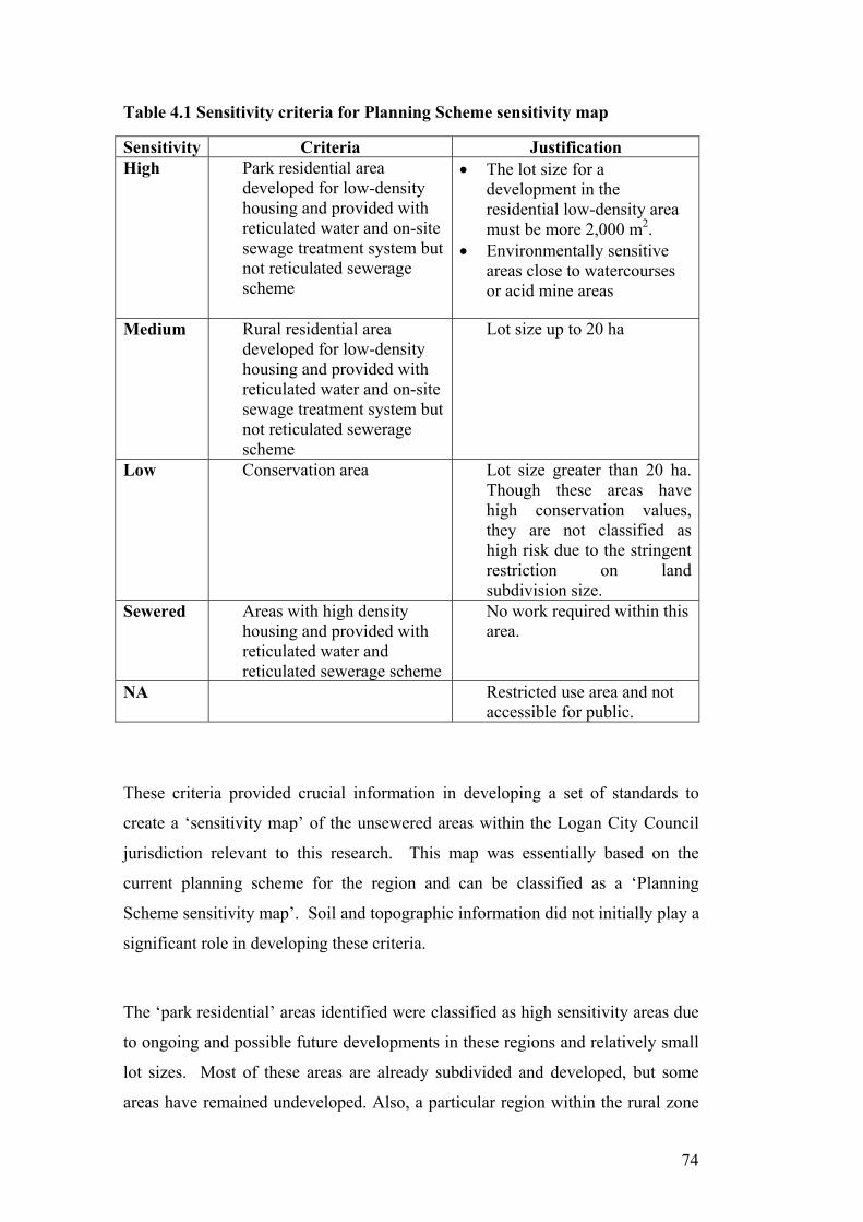
74

Table 4.1 Sensitivity criteria for Planning Scheme sensitivity map

Sensitivity Criteria Justification High Park residential area

developed for low-density housing and provided with reticulated water and on-site sewage treatment system but not reticulated sewerage scheme

• The lot size for a development in the residential low-density area must be more 2,000 m2.

• Environmentally sensitive areas close to watercourses or acid mine areas

Medium Rural residential area developed for low-density housing and provided with reticulated water and on-site sewage treatment system but not reticulated sewerage scheme

Lot size up to 20 ha

Low Conservation area Lot size greater than 20 ha. Though these areas have high conservation values, they are not classified as high risk due to the stringent restriction on land subdivision size.

Sewered Areas with high density housing and provided with reticulated water and reticulated sewerage scheme

No work required within this area.

NA Restricted use area and not accessible for public.

These criteria provided crucial information in developing a set of standards to

create a ‘sensitivity map’ of the unsewered areas within the Logan City Council

jurisdiction relevant to this research. This map was essentially based on the

current planning scheme for the region and can be classified as a ‘Planning

Scheme sensitivity map’. Soil and topographic information did not initially play a

significant role in developing these criteria.

The ‘park residential’ areas identified were classified as high sensitivity areas due

to ongoing and possible future developments in these regions and relatively small

lot sizes. Most of these areas are already subdivided and developed, but some

areas have remained undeveloped. Also, a particular region within the rural zone

75

has been identified as a high sensitivity area for residential and commercial

development on the Planning Scheme map. This refers to the Berrinba area, which

lies within the unsewered area. The area has significant environmental values, and

LCC could choose not to extend sewers into the area to ensure that the area will

not be developed too intensely.

The medium sensitivity areas mostly consisted of ‘rural’ areas, some with

conservation value. However, there were some pockets within these areas that

required special attention due to environmental sensitivity or cultural heritage

values. The low sensitivity areas were intended to stay rural. The Planning

Scheme sensitivity map that was developed is shown in Figure 4.2.

4.3.2 Field Investigations

On completion of the desktop study and producing the planning scheme

sensitivity map, the field investigation of selected sites for soil sampling was

undertaken. The field sampling commenced by developing two checklists to be

used for each sampled site. These checklists were developed to obtain preliminary

information about the sites and to assist in deciding on the priority level of the

sites based on the criteria developed in Table 4.1. The checklists are given in

Appendix C.

76

Kilometres

Figure 4.2 Planning scheme sensitivity zones for Logan City Council region

77

Checklist A (Appendix C) was used to record the site description needed for the

subsequent sampling data analysis. Site description was among the important

information needed for each site. The information collected included topography,

location of the landscape catena (White, 1997), vegetation, current land use, and

soil type. The developed planning scheme sensitivity map and checklist

completed the preparation necessary for the preliminary site selection, thereby

allowing the fieldwork to be undertaken.

Another checklist was developed for the field sites sampling and description

(Checklist B see Appendix C) to maintain a record for the sampled sites, and help

in the subsequent soil physico-chemical evaluation. This checklist included the

sampling data and the coordinates of the selected sites, which were noted using a

Global Positioning System (GPS). In addition, the checklist contained the current

street directory maps for plotting and locating purposes, number of soil samples

collected from each sampling point and planning sensitivity level. Also, the

expected soil type was identified based on the available soil maps. The actual soil

type was based on the Australian Soil Classification (Jacquier et al., 2000), which

was undertaken in the field and the soil profile descriptions were included in the

checklist

The fieldwork was divided into two phases. Preliminary site selection was the first

phase and detailed site selection was the second phase. In the first phase, or the

broad scale sampling, site selection was based on the developed planning scheme

sensitivity map (Figure 4.2) and the sensitivity criteria (Table 4.1). Preliminary

site selection primarily focused on the high sensitivity areas using a grid sampling

system at intervals of approximately 1 km. Sites in the medium sensitivity

planning areas were selected based on a change of soil type or a separation

distance of about 1.5 km between each two sites. In areas with low sensitivity,

the sites were selected based on changes in the soil types or a separation distance

of every 2.5 km. Twenty-nine sites were selected in the preliminary site selection

stage, and the location of these sites with the GPS coordinates are given in Table

4.2. In addition, the sites are indicated on the planning scheme sensitivity map as


78

Table 4.2 Site location and GPS coordinates for the preliminary investigation

stage

GPS Coordinates Site

No.

locality

Northing Easting

Level of

Sensitivity

1 Park Ridge 509180 6935053 High2 Park Ridge 507708 6935298 High3 Park Ridge 505806 6935893 High4 Park Ridge 504658 6936078 High5 Park Ridge 504124 6936179 High6 Park Ridge 500283 6936106 High7 Park Ridge 500787 6935532 High8 Park Ridge South 499000 6933718 Moderate 9 Park Ridge South 500214 6933512 Moderate 10 Park Ridge South 501747 6933426 Moderate 11 Park Ridge 503637 6934248 Moderate 12 Park Ridge 505306 6933995 Moderate 13 Berrinba 506618 6933926 Moderate 14 Park Ridge 508273 6933702 Moderate 15 Logan Reserve 511498 6934860 Low16 Logan Reserve 510623 6934775 Low17 Logan Reserve 511135 6935500 Low18 Park Ridge 491342 3762160 Low19 Park Ridge 508108 6936284 High20 Park Ridge 507061 6936781 High21 Regents Park 503962 6937373 High22 Forestdale 502869 6960578 High23 Forestdale 499571 6939969 High24 Forestdale 500373 6939863 High25 Berrinba 500742 6940680 High26 Berrinba 508008 6941032 High27 Berrinba 508271 6940478 High28 Cornubia 522060 6940843 High29 Mount Cotton 520566 6942916 Low

The 29 selected sites contained 17 sites from the high sensitivity areas, seven from

the medium sensitivity areas and five sites from the low sensitivity areas. A total

of 93 soil samples were collected representing the different soil horizons from

each of the selected 29 sites.

The second phase in the site selection process formed a refinement of the

preliminary site selection. The fundamental difference between the two phases of

site selection was the use of data from the preliminary soil physico-chemical

79

analysis and evaluation, which were incorporated into the subsequent site

selection. The results of the soil sampling from the first phase were used to

support the second phase of site selection. In the detailed site selection phase, it

was necessary to verify the preliminary information derived from the initial phase.

The physico-chemical analysis derived from the first phase raised issues and

questions that needed to be clarified. For instance, some sites showed a high level

of organic nitrogen, while other sites were found to have a low cation exchange

capacity. The results that raised questions prompted the need to locate extra

sampling sites in selected areas for the purpose of verification and analysis. A

total of additional 19 sites were located and sampled as reported in Table 4.3. Ten

of these sites were in the low sensitivity areas and nine sites in the high sensitive

areas, which are shown in Figure 4.3. Forty-six soil samples were collected from

the 19 sites representing the different soil horizons to be analysed.

Table 4.3 Location of the selected sites in the detailed stage

GPS CoordinatesSite No Locality Northing Easting

Level of Sensitivity

30 Browns Plains 507285 6941007 High 31 Berrinba 507527 6941042 High 32 Hillcrest 491342 3762160 High 33 Forestdale 500324 6940768 High 34 Daisy Hill 515142 6944893 Low35 Daisy Hill 514570 6944043 Low36 Daisy Hill 515563 6944306 Low37 Carbrook 521152 6939935 High 38 Carbrook 522109 6939856 High 39 Cornubia 521774 6940769 High 40 Mount Cotton 520831 6941697 Low41 Cornubia 520892 6941534 Low42 Cornubia 520359 6940793 Low43 Park Ridge 520137 6940909 Low44 Logan Reserve 509431 6935451 High 45 Carbrook 509427 6935451 High 46 Carbrook 524221 6938348 Low47 Carbrook 526058 6937421 Low48 Redland Bay 527672 6937361 Low

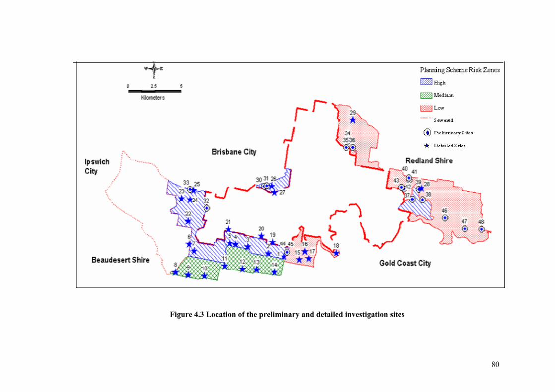
80

Figure 4.3 Location of the preliminary and detailed investigation sites

81

4.4 Soil Sampling The sampling process was conducted in a consistent manner to ensure accuracy of

the soil analysis undertaken. This entailed the development of a protocol for soil

sample collection to cover all the necessary measures to obtain representative

samples from the sites.

4.4.1 Procedures

A hand auger of 100 mm diameter was used to collect the soil samples. The

following procedures and measures were adapted for each site:

1. Sampling site descriptions were noted in Checklist B (Appendix C) such as

location, the ground conditions and landscape factors, existing structures

around the site and land use;

2. The samples were collected at least 10 m away from the side of the road (for

easy access) and to ensure that the soil was not disturbed;

3. The waterways were another important factor determining the location of

sampling sites,with at least 200 m separation from any waterways to ensure

that the soil was not disturbed by water movement;

4. The site coordinates were recorded for each site using a GPS and the closest

street address was recorded;

5. The depth of sampling was required to be at least 800 mm and up to 1400 mm

at each site;

6. Soil samples representing each horizon were collected on a plastic sheet and

mixed thoroughly to ensure homogeneity, and a one kilogram sample was

collected and stored in a sealed plastic bag for laboratory testing;

7. All samples were labelled with a unique identifier, which included the site

number, the street address, the horizon and the date of sampling;

8. The change of soil horizon was recorded on a soil profile sheet by measuring

the depth, and the soil characteristics at that depth were described;

9. Subsurface profiles for each site were mapped at a suitable road cutting;

10. The soil profile was used to determine the actual soil type by comparing it to

the Australian Soil Classification (Jacquier et al., 2000); and

11. Photographs of each sampled site, soil profile and vegetation in the area were

taken for records and further analysis.

82

The field sampling procedures are illustrated in Figure 4.4 showing the soil

collected from the different soil horizons. Figure 4.5 illustrates how the soil depth

was measured for each site. The soil classification was based on the soil samples

collected from a site combined with information from a profile cut such as a road

excavation. Figure 4.6 illustrates a typical road cut.

4.4.2 Sample Preparation and Handling

In general, preliminary preparation of all soil samples was undertaken before any

further physico-chemical analysis was considered. The following preliminary

preparation and measures were applied for all the soil samples:

• Samples were oven dried at 50oC to maintain the same moisture level for all

soil samples;

• Gravel was removed using a 2.36 mm sieve, and the remaining material was

ground to less than 2.36 mm; and

• The samples were kept at room temperature.

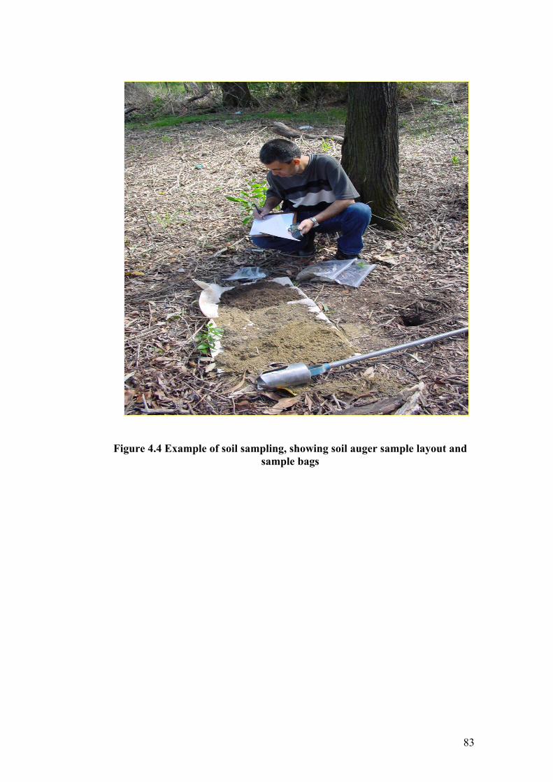
83

Figure 4.4 Example of soil sampling, showing soil auger sample layout and sample bags

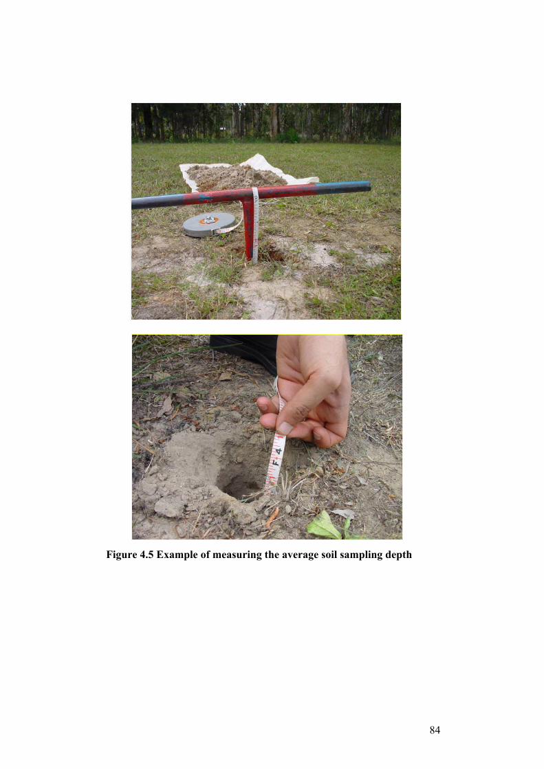
84

Figure 4.5 Example of measuring the average soil sampling depth

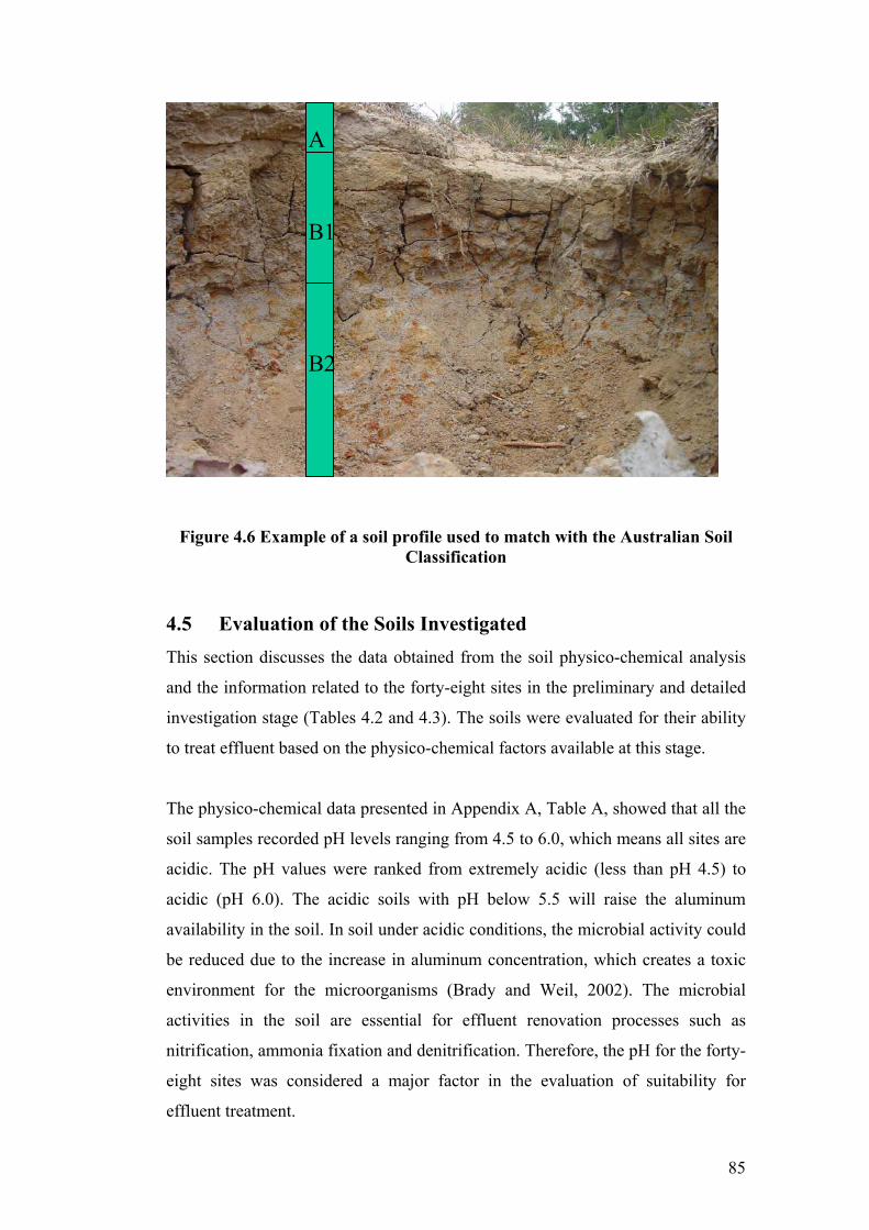
85

Figure 4.6 Example of a soil profile used to match with the Australian Soil Classification

4.5 Evaluation of the Soils Investigated This section discusses the data obtained from the soil physico-chemical analysis

and the information related to the forty-eight sites in the preliminary and detailed

investigation stage (Tables 4.2 and 4.3). The soils were evaluated for their ability

to treat effluent based on the physico-chemical factors available at this stage.

The physico-chemical data presented in Appendix A, Table A, showed that all the

soil samples recorded pH levels ranging from 4.5 to 6.0, which means all sites are

acidic. The pH values were ranked from extremely acidic (less than pH 4.5) to

acidic (pH 6.0). The acidic soils with pH below 5.5 will raise the aluminum

availability in the soil. In soil under acidic conditions, the microbial activity could

be reduced due to the increase in aluminum concentration, which creates a toxic

environment for the microorganisms (Brady and Weil, 2002). The microbial

activities in the soil are essential for effluent renovation processes such as

nitrification, ammonia fixation and denitrification. Therefore, the pH for the forty-

eight sites was considered a major factor in the evaluation of suitability for

effluent treatment.

A

B1

B2

A

B1

B2

A

B1

B2

86

Soils are considered to have salinity problems when the concentration of soluble

salts is high enough to affect plant growth. The salinity levels for soils can be

classified as saline, saline-sodic or non saline-sodic, depending on the chemical

composition of the salts (Shaw et al., 1987). Electrical conductivity was measured

for all sites, and the range was from 10 to 105 µS/cm. In general, the values of EC

in these soils were in the normal range (EC < 4 dS/m), (1 dS/m= 1000µS/cm)

when compared to the general values for Australian soils. Effluent application

contributes strongly to the EC if the soil has the capacity to attract the free ions in

the effluent. The salts are mainly chlorides and sulfates of calcium, magnesium,

potassium and sodium. The increase of the EC to values greater than 4 dS/m and

exchangeable sodium percentage (ESP) values less than 15% could lead to

salinity problems, especially if the soil pH is below 8.5 (Brady and Weil, 2002).

According to the EC values obtained, all investigated sites were considered to be

non saline-non sodic (normal) soils. However, as these soils have a pH less than

8.5, as a result of effluent application the soil alkalinity will rise and could lead to

a salinity problem in the future.

Chloride mostly exists in a soluble form in the soil and is considered to be a good

indicator of the soil leaching capacity and as a salinity indicator (Brady and Weil,

2002). Chloride was used in the study as an indicator for the soil leaching

capacity. Low Cl- concentrations can be attributed to two reasons: the soil has a

coarse texture with a high permeability and low CEC, or it is a fine textured soil

with a heavy clay content and very low permeability (Khalil et al., 2003). In the

case of heavy clay, the Cl- will accumulate mostly in the first few centimetres of

the finer textured layer. Therefore, using Cl- as an indicator to evaluate the soil

permeability is associated with the soil mineralogy and the subsurface hydrology

(Shaw et al., 1987). The Cl- concentrations measured were in the range between 5

and 100 mg/Kg.

The source of organic matter in the soil was mostly from the added plant and

animal debris. The presence of OM is of great importance in the formation and

stabilisation of soil structure. OM in the soil is considered an important factor

contributing to the CEC, especially in the sandy soils. Most of the soil OM

adheres strongly to the mineral particles (humification), particularly in clay to

87

form a clay-humus complex. This colloid produces a high specific surface area

and high CEC. Organic matter can act as a source of nutrients to the plants

through various release and uptake mechanisms (Mitchell, 1932). The

investigated sites exhibited variations in OM between 1 and 12%. The OM in

most soils decreased down the soil profile but in some cases there was no clear

trend. Soil OM are affected by moisture, oxygen, temperature and pH. The first

two factors tend to counteract one another because when soil moisture is high,

deficiency of O2 may restrict organic matter decomposition, whereas when the soil

is dry, moisture but not O2 will be the limiting factor. pH has little effect, except

below 4 when the decomposition is slow. On the other hand, temperature has a

marked effect, not only on plant growth, but also on the waste decomposition

through an effect on microbial respiration rate (Jenkinson and Ayanaba, 1977)

Nitrogen and phosphorus were measured at each site (Appendix A, Table A). The

nitrogen concentration in the forty-eight sites was measured as NH3-N and the

concentrations measured were in the range between 10 and 400 mg/Kg. The

highest nitrogen concentrations were reported at Sites 1 and 2 (Table 4.2). These

sites were located close to nurseries in the Park Ridge area where large amounts

of fertilisers are used.

Phosphorus was measured in the form of orthophosphate (PO43-) and the

concentrations were in the range between 0.1 to 13 mg/Kg. Most of the

investigated sites reported low phosphorus content. Measurement of the nutrients

available in the soil is an important factor in managing the soil’s nutrient holding

capacity. In the case of continuous effluent application, the nutrient level in the

soil is expected to increase. This increase of nutrient level is controlled by the soil

mineralisation and sorption capacity (White, 1997). Soils with weak capacity to

hold nutrients have the potential to lose these nutrients by leaching them to the

groundwater.

CEC is an expression of the negative charge per unit mass of soil (meq/100g).

The crystalline framework of the clay minerals (such as kaolinite, illite and

smectite) acts as a reservoir for the cations released by weathering and organic

decomposition, which are adsorbed by clay and organic colloids, leaving low

88

cations concentration in the soil solution to be balanced by mineral anions and

biocarbonate generated from the respiration of the soil organisms. The CEC levels

vary depending on the clay type and content and organic matter content. The

CEC for the different sites at various soil horizons varied between 2 and 86

meq/100g.

The exchangeable sodium percentage (ESP) in the soil is an indicator to evaluate

the possible hazard created by increasing the soil sodicity due to effluent

application and water irrigation (Ahern et al., 1988). The data presented in

Appendix A, Table C, give the concentrations for six individual exchangeable

cations, namely, Ca2+, Mg2+, Na+, K+, Al3+ and Fe3+ for the forty-eight sites. These

data were used to calculate ESP based on the CEC. The ESP values are calculated

based on (ESP = (exchangeable Na/CEC) x 100%) and the data is expressed as a

percentage. The soil sodicity has been rated by Northcote and Skene (1972)

where ESP < 6% is considered non-sodic, ESP = 6-15% is sodic, and ESP > 15%

is strongly sodic. The values for ESP given in Appendix A, Table C show that the

ESP for the forty-eight sites were non-sodic (ESP < 6%). The increase of salts

concentration in soil will lead to an increase in ESP and the level of sodicity could

also increase with depth. ESP has a significant impact on the soil physical

properties. The soil will lose aggregation and develop clay dispersion leading to

high permeability and formation of a surface crust if it has a strongly-sodic ESP.

However, this will create unsatisfactory conditions for effluent application and

adversely affect the soil’s ability to transmit and renovate effluent.

4.6 Description of Soil Orders A total of nine soil orders were determined for the forty-eight sites investigated

according to the Australian Soil Classification (Isbell, 1996) (Table 4.4), and

based on the outcomes of the field observations. The physico-chemical data for

these soils are reported in Appendix A, Table A and the mineralogical data

analysis in Table B, Appendix A.

4.6.1 Dermosol Soil

Fourteen out of the forty-eight investigated sites were Dermosols. The Dermosol

is characterised by structured B2-horizons and lacks strong texture contrast

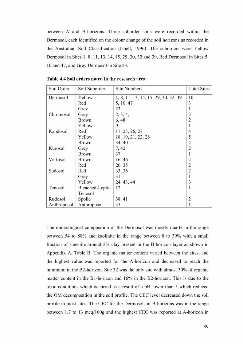
89

between A and B-horizons. Three suborder soils were recorded within the

Dermosol, each identified on the colour change of the soil horizons as recorded in

the Australian Soil Classification (Isbell, 1996). The suborders were Yellow

Dermosol in Sites 1, 8, 11, 13, 14, 15, 29, 30, 32 and 39, Red Dermosol in Sites 5,

10 and 47, and Grey Dermosol in Site 23.

Table 4.4 Soil orders noted in the research area

Soil Order Soil Suborder Site Numbers Total Sites

Dermosol Chromosol Kandosol Kurosol Vertosol Sodosol Tenosol Rudosol Anthroposol

Yellow Red Grey Grey Brown Yellow Red Yellow Brown Grey Brown Brown Red Red Grey Yellow Bleached-Leptic Tenosol Spolic Anthroposol

1, 8, 11, 13, 14, 15, 29, 30, 32, 39 5, 10, 47 23 2, 3, 4, 6, 48 9 17, 25, 26, 27 18, 19, 21, 22, 28 34, 40 7, 42 37 16, 46 20, 35 33, 36 31 24, 43, 44 12 38, 41 45

10 3 1 3 2 1 4 5 2 2 1 2 2 2 1 3 1 2 1

The mineralogical composition of the Dermosol was mostly quartz in the range

between 54 to 88% and kaolinite in the range between 8 to 39% with a small

fraction of smectite around 2% clay present in the B-horizon layer as shown in

Appendix A, Table B. The organic matter content varied between the sites, and

the highest value was reported for the A-horizon and decreased to reach the

minimum in the B2-horizon. Site 32 was the only site with almost 30% of organic

matter content in the B1-horizon and 16% in the B2-horizon. This is due to the

toxic conditions which occurred as a result of a pH lower than 5 which reduced

the OM decomposition in the soil profile. The CEC level decreased down the soil

profile in most sites. The CEC for the Dermosols at B-horizons was in the range

between 1.7 to 13 meq/100g and the highest CEC was reported at A-horizon in

90

Site 1. The CEC is pH dependent and this site has a pH over 5 and organic content

around 8.7%. The OM contributed positively to the CEC level. pH was reported in

the range from 4.3 to 6.3 for the Yellow Dermosol, from 4.7 to 5.9 for the Red

Dermosol, and 5.2 for the Grey Dermosol. Once the soil pH is below 5.5

aluminosilicate clays and Al3+ hydroxide minerals begin to dissolve, releasing Al-

hydroxy cations and Al3+ that then exchange other cations from soil colloids

(McBride, 1994). The sites which are occupied by Al3+ can increase as pH is

decreased lower than 5, and the concentration of soluble Al will build up if the pH

is lowered more (McBride, 1994). The presence of a higher concentration of

soluble Al3+ will result in a harmful effect on microorganism activity in the soil.

The pH increased down the soil profile in Sites 8, 13, 29 and 30 and decreased in

Sites 1, 14, 15 and the other sites have an unstable trend of pH values as a result

of soluble salts concentrations. The ESP for the Dermosol was mostly reported

within the non-sodic range due to the low soluble salts in the soil.

4.6.2 Chromosol Soil

Chromosols were found in six sites and could be divided into three suborders:

Grey Chromosol in Sites 2, 3 and 4, Brown Chromosol in Sites 6 and 48, and

Yellow Chromosol in Site 9. In general, this soil order is characterised by a strong

textural contrast between the A-horizon and the B-horizon.

The Chromosols mineralogy was dominated by kaolinite clay of almost 50% of

the total soil composition and the rest was 43% quartz and 5% amorphous

material with a small amount of illite. Kaolinite is the least active clay which does

not swell in water except in extremely polar solvents and it has low surface area

and CEC. The high content of kaolinite associated with the illite clay and OM

were the main contributors to the CEC level available in the soil. The OM was

lower than in the Dermosols and decreased down the profile in the investigated

sites. The CEC levels were the lowest in the A-horizon and the highest in the B2-

horizon with an average of 26 meq/100g. This had a pH in the range 4.7 to 5.9.

This soil has low soluble salts content and most of the salts in the soil were in the

chloride form. Phosphorus content was the highest in the B2-horizon in most of

the investigated sites. The individual exchangeable cations indicated that the

dominant cations were Mg2+ followed by Na+ and Ca2+. The soil Ca:Mg ratios

91

were less than 0.5 at B-horizons, which could be due to the Na+ and Mg2+ being

able to depress the Ca2+ activity. The reduction of the Na+ activity and the

increase of Ca2+ will improve the soil fertility (Baker and Eldershaw, 1993). The

soils’ ESP was non-sodic in most investigated soils due to the low Na+

concentrations.

4.6.3 Kandosol Soil

Eleven sites were noted as having Kandosols. Three suborder soils were observed:

Red Kandosol in Sites 17, 25, 26 and 27, Yellow Kandosol in Sites 18, 19, 21, 22

and 28, and Brown Kandosol in Sites 34 and 40. Kandosols include soils which

lack strong textural contrast, and have massive or weakly structured B-horizons.

The soil mineralogy for the kandosols indicated that the dominant clay type

kaolinite 40% with more than 10% illite in the B-horizons, 40% quartz and the

rest was amorphous material. The physico-chemical data for the Kandosols are

reported in Appendix A, Table A. OM decreased down the soil profile in most of

the investigated sites except Sites 25 and 34 where there was a small increase in

the B2- horizon that could be due to OM deposition. Also, the OM with the small

portion of illite at A-horizon increased the CEC level at these layers. The CEC

levels ranged between 26 and 88 meq/100g at B-horizon; the higher values were

reported at B1-horizon and lower values reported at B2-horizon due to the weak

structure at B2-horizons. The OM and the illite content improved the total clay

CEC especially in the B-horizons. pH ranged between 4.2 and 5.8, and soil acidity

increased with depth in most of the investigated sites. The individual

exchangeable cations for the investigated sites indicated a low Mg2+ concentration

at the A-horizons with a constant increase down the soil profile; Ca2+

concentrations were low at the A-horizon and decreased down to the B2-horizon.

Na+ and Mg2+ concentrations were almost consistent values from the A to the B-

horizons. There was a presence of Al3+ associated with K+, which was due to low

acidity down the profile and which will increase the release of soluble Al3+ from

the octahedral sheet (McBride, 1994). The soils have low Ca:Mg values (low

fertility) and low ESP (non-sodic) which means low activity of the Ca+ and high

CEC level controlling the soil fertility and the ESP in the soil. The soluble salts

were low in all sites except at sites 34, 40 and 47 as a result of high kaolinite

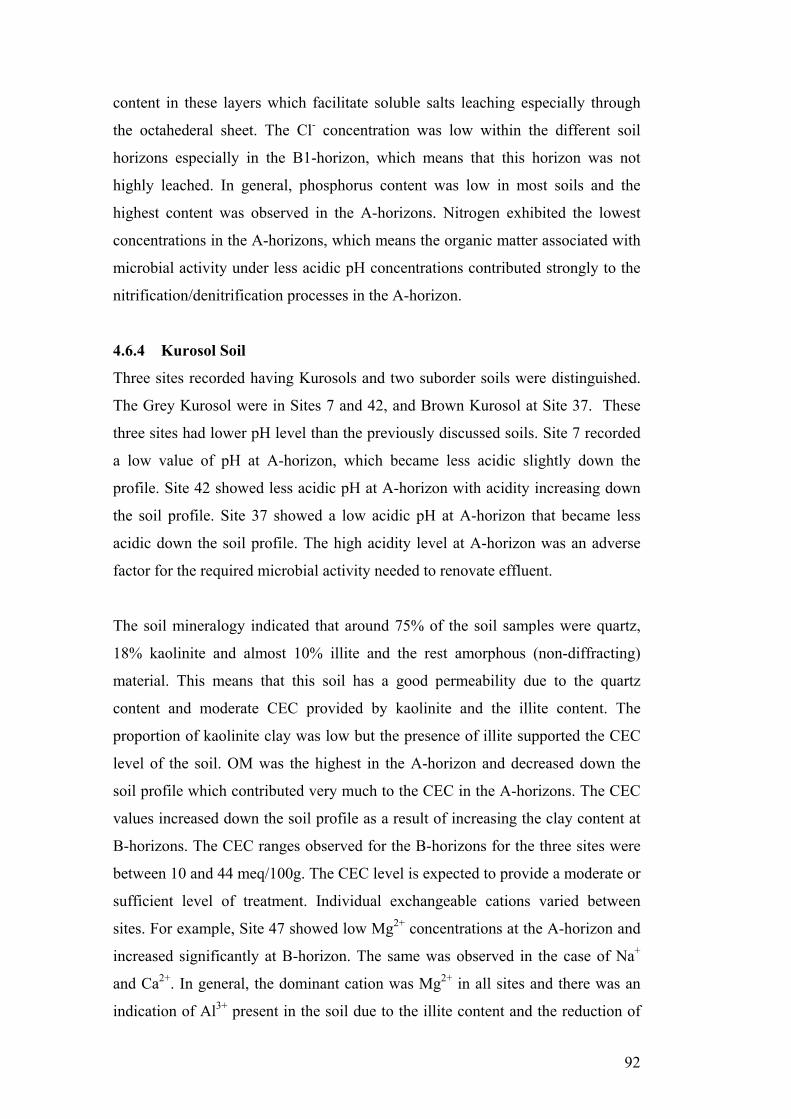
92

content in these layers which facilitate soluble salts leaching especially through

the octahederal sheet. The Cl- concentration was low within the different soil

horizons especially in the B1-horizon, which means that this horizon was not

highly leached. In general, phosphorus content was low in most soils and the

highest content was observed in the A-horizons. Nitrogen exhibited the lowest

concentrations in the A-horizons, which means the organic matter associated with

microbial activity under less acidic pH concentrations contributed strongly to the

nitrification/denitrification processes in the A-horizon.

4.6.4 Kurosol Soil

Three sites recorded having Kurosols and two suborder soils were distinguished.

The Grey Kurosol were in Sites 7 and 42, and Brown Kurosol at Site 37. These

three sites had lower pH level than the previously discussed soils. Site 7 recorded

a low value of pH at A-horizon, which became less acidic slightly down the

profile. Site 42 showed less acidic pH at A-horizon with acidity increasing down

the soil profile. Site 37 showed a low acidic pH at A-horizon that became less

acidic down the soil profile. The high acidity level at A-horizon was an adverse

factor for the required microbial activity needed to renovate effluent.

The soil mineralogy indicated that around 75% of the soil samples were quartz,

18% kaolinite and almost 10% illite and the rest amorphous (non-diffracting)

material. This means that this soil has a good permeability due to the quartz

content and moderate CEC provided by kaolinite and the illite content. The

proportion of kaolinite clay was low but the presence of illite supported the CEC

level of the soil. OM was the highest in the A-horizon and decreased down the

soil profile which contributed very much to the CEC in the A-horizons. The CEC

values increased down the soil profile as a result of increasing the clay content at

B-horizons. The CEC ranges observed for the B-horizons for the three sites were

between 10 and 44 meq/100g. The CEC level is expected to provide a moderate or

sufficient level of treatment. Individual exchangeable cations varied between

sites. For example, Site 47 showed low Mg2+ concentrations at the A-horizon and

increased significantly at B-horizon. The same was observed in the case of Na+

and Ca2+. In general, the dominant cation was Mg2+ in all sites and there was an

indication of Al3+ present in the soil due to the illite content and the reduction of

93

pH levels down the soil profile. This soil has a low fertility (Mg:Ca less than 0.5)

and a non-sodic ESP soil as a result of the low soluble salts content at A-horizons.

The soluble salts decreased down the soil profile at Sites 7 and 37 as a result of

the higher pH at B-horizons. EC increased down the soil profile at Site 42 as a

result of pH decrease from 5.1 at A-horizon to higher acidity at B-horizon (pH

4.6). Low phosphorus content was recorded in the A-horizon and decreased down

the soil profile as a result of low organic content which reduced the phosphorus

uptake level.

4.6.5 Vertosol Soil

This soil was observed in four sites and there were two suborder soil types

distinguished. The first suborder was Brown Vertosol in Sites 16 and 46 and the

second suborder was Red Vertosol in Sites 20 and 35.

The soil mineralogy analysis indicated that the dominant clay was kaolinite with a

content of 40%. The investigated sites exhibited acidic soils with pH values

between 4.6 and 5.2. The acidic conditions resulted in incease of Al3+

concentration level from 0.02 to 0.03 meq/100g in the soil as shown in Appendix

A Table C. OM increased down the soil profile as a result of low organic matter

decomposition due to the slow microbial activity. Also, the CEC level increased

down the soil profile due to the increase of kaolinite and OM. The individual

exchangeable cations indicated that the dominant cations were Mg2+ and Na+ with

an almost consistent level down the soil profile. The Ca2+ decreased and Mg2+

increased down the soil profile. The increase of Mg2+ inhibited the increase of

Ca2+. Phosphorus content increased down the soil profile especially in Sites 16

and 20 as a result of the increase in OM which improved the phosphorus uptake.

Also, the nitrogen level increased down the soil profile due to the increase of OM

which increased the nitrogen fixation level. The Cl- ions increased down the

profile slightly, but the value of Cl- were low compared to the Kurosols. This is an

indication of the poor Cl- ion mobility in the soil, which means the soil has a low

leached profile due to the high clay content in the soil (Khalil et al., 2003). The

soil reported a low Ca:Mg ratio of less than 0.5 as a result of imbalance between

the Ca2+ and Mg2+ (Powell, 1982). This soil is considered a non-sodic soil as ESP

reported was less than 6%. This is due to the soluble salts in the soil.

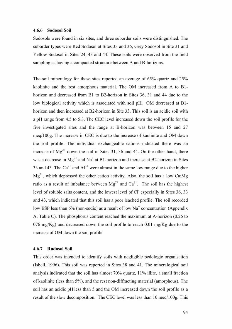
94

4.6.6 Sodosol Soil

Sodosols were found in six sites, and three suborder soils were distinguished. The

suborder types were Red Sodosol at Sites 33 and 36, Grey Sodosol in Site 31 and

Yellow Sodosol in Sites 24, 43 and 44. These soils were observed from the field

sampling as having a compacted structure between A and B-horizons.

The soil mineralogy for these sites reported an average of 65% quartz and 25%

kaolinite and the rest amorphous material. The OM increased from A to B1-

horizon and decreased from B1 to B2-horizon in Sites 36, 31 and 44 due to the

low biological activity which is associated with soil pH. OM decreased at B1-

horizon and then increased at B2-horizon in Site 33. This soil is an acidic soil with

a pH range from 4.5 to 5.3. The CEC level increased down the soil profile for the

five investigated sites and the range at B-horizon was between 15 and 27

meq/100g. The increase in CEC is due to the increase of kaolinite and OM down

the soil profile. The individual exchangeable cations indicated there was an

increase of Mg2+ down the soil in Sites 31, 36 and 44. On the other hand, there

was a decrease in Mg2+ and Na+ at B1-horizon and increase at B2-horizon in Sites

33 and 43. The Ca2+ and Al3+ were almost in the same low range due to the higher

Mg2+, which depressed the other cation activity. Also, the soil has a low Ca:Mg

ratio as a result of imbalance between Mg2+ and Ca2+. The soil has the highest

level of soluble salts content, and the lowest level of Cl- especially in Sites 36, 33

and 43, which indicated that this soil has a poor leached profile. The soil recorded

low ESP less than 6% (non-sodic) as a result of low Na+ concentration (Appendix

A, Table C). The phosphorus content reached the maximum at A-horizon (0.26 to

076 mg/Kg) and decreased down the soil profile to reach 0.01 mg/Kg due to the

increase of OM down the soil profile.

4.6.7 Rudosol Soil

This order was intended to identify soils with negligible pedologic organisation

(Isbell, 1996). This soil was reported in Sites 38 and 41. The mineralogical soil

analysis indicated that the soil has almost 70% quartz, 11% illite, a small fraction

of kaolinite (less than 5%), and the rest non-diffracting material (amorphous). The

soil has an acidic pH less than 5 and the OM increased down the soil profile as a

result of the slow decomposition. The CEC level was less than 10 meq/100g. This

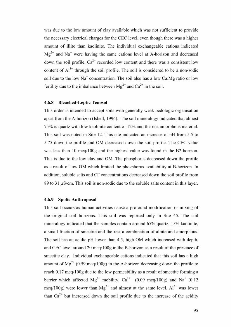
95

was due to the low amount of clay available which was not sufficient to provide

the necessary electrical charges for the CEC level, even though there was a higher

amount of illite than kaolinite. The individual exchangeable cations indicated

Mg2+ and Na+ were having the same cations level at A-horizon and decreased

down the soil profile. Ca2+ recorded low content and there was a consistent low

content of Al3+ through the soil profile. The soil is considered to be a non-sodic

soil due to the low Na+ concentration. The soil also has a low Ca:Mg ratio or low

fertility due to the imbalance between Mg2+ and Ca2+ in the soil.

4.6.8 Bleached-Leptic Tenosol

This order is intended to accept soils with generally weak pedologic organisation

apart from the A-horizon (Isbell, 1996). The soil mineralogy indicated that almost

75% is quartz with low kaolinite content of 12% and the rest amorphous material.

This soil was noted in Site 12. This site indicated an increase of pH from 5.5 to

5.75 down the profile and OM decreased down the soil profile. The CEC value

was less than 10 meq/100g and the highest value was found in the B2-horizon.

This is due to the low clay and OM. The phosphorus decreased down the profile

as a result of low OM which limited the phosphorus availability at B-horizon. In

addition, soluble salts and Cl- concentrations decreased down the soil profile from

89 to 31 μS/cm. This soil is non-sodic due to the soluble salts content in this layer.

4.6.9 Spolic Anthroposol

This soil occurs as human activities cause a profound modification or mixing of

the original soil horizons. This soil was reported only in Site 45. The soil

mineralogy indicated that the samples contain around 65% quartz, 15% kaolinite,

a small fraction of smectite and the rest a combination of albite and amorphous.

The soil has an acidic pH lower than 4.5, high OM which increased with depth,

and CEC level around 20 meq/100g in the B-horizon as a result of the presence of

smectite clay. Individual exchangeable cations indicated that this soil has a high

amount of Mg2+ (0.59 meq/100g) in the A-horizon decreasing down the profile to

reach 0.17 meq/100g due to the low permeability as a result of smectite forming a

barrier which affected Mg2+ mobility. Ca2+ (0.09 meq/100g) and Na+ (0.12

meq/100g) were lower than Mg2+ and almost at the same level. Al3+ was lower

than Ca2+ but increased down the soil profile due to the increase of the acidity

96

level. Nitrogen increased down the soil profile and phosphorus recorded the same

level (0.28 meq/100g) at A and B-horizons. The soluble salts content increased

and reached the maximum at B2-horizon. Cl- concentration increased with depth,

which means that the soil has a low permeability (Khalil et al., 2003). This soil is

non-sodic due to the Na+ concentration.

4.7 Conclusions Site selection and field sampling were among the most critical stages of the

research. Developing the criteria for site selection increased the work efficiency

by focusing on the sensitive areas. The preliminary investigation stage was the

implementation of the desktop study. This stage of investigation raised many

issues related to the soil in the area. To answer these questions, a further detailed

investigation stage was conducted.

The nine soil orders were distinguished in the course of the undertaken analysis.

Summary outcomes of the nine soil orders are tabulated in Table 4.5.

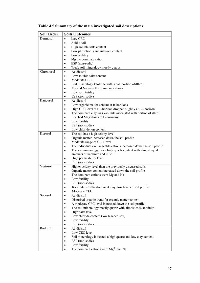
97

Table 4.5 Summary of the main investigated soil descriptions

Soil Order Soils Outcomes Dermosol • Low CEC

• Acidic soil • High soluble salts content • Low phosphorus and nitrogen content • Low fertility • Mg the dominate cation • ESP (non-sodic) • Weak soil mineralogy mostly quartz

Chromosol • Acidic soil • Low soluble salts content • Moderate CEC • Soil mineralogy kaolinite with small portion ofiIllite • Mg and Na were the dominant cations • Low soil fertility • ESP (non-sodic)

Kandosol • Acidic soil • Low organic matter content at B-horizons • High CEC level at B1-horizon dropped slightly at B2-horizon • The dominant clay was kaolinite associated with portion of illite • Leached Mg cations to B-horizons • Low fertility • ESP (non-sodic) • Low chloride ion content

Kurosol • The soil has a high acidity level • Organic matter increased down the soil profile • Moderate range of CEC level • The individual exchangeable cations increased down the soil profile • The soil mineralogy has a high quartz content with almost equal

amounts of kaolinite and illite • High permeability level • ESP (non-sodic)

Vertosol • Higher acidity level than the previously discussed soils • Organic matter content increased down the soil profile • The dominant cations were Mg and Na • Low fertility • ESP (non-sodic) • Kaolinite was the dominant clay; low leached soil profile • Moderate CEC

Sodosol • Acidic soil • Disturbed organic trend for organic matter content • A moderate CEC level increased down the soil profile • The soil mineralogy mostly quartz with almost 25% kaolinite • High salts level • Low chloride content (low leached soil) • Low fertility • ESP (non-sodic)

Rudosol • Acidic soil • Low CEC level • Soil mineralogy indicated a high quartz and low clay content • ESP (non-sodic) • Low fertility • The dominant cations were Mg2+ and Na+

98

Bleached-Leptic Tenosol

• Acidic soil with pH increased down the soil profile • Low organic content which was decreased down the soil profile • Low CEC level • Soluble salts decreased down the soil profile • Chloride ion decreased down the soil profile • Low fertility • ESP (non-sodic)

Spolic Anthroposol

• Low acidity level • Moderate CEC level • High organic matter in all horizons • Highly leached soil profile • Al cations availability created toxic conditions for the microbial activity • ESP (non-sodic)

99

Chapter 5 Experimental Study on Vertical Effluent

Transport in Soils

5.1 Overview There exists a shortage of information about the performance of soils under

effluent application. A laboratory experiment was designed to study the vertical

transport of effluent through the various soils present in the research area. The

soil column experiment was designed to understand the actual soil behaviour in

the subsurface effluent disposal area. The changes that occurred in the soil

physico-chemical characteristics after effluent application were investigated to

validate the outcomes obtained from the field investigation and to fill the gaps in

the scientific knowledge in relation to soil performance under effluent application.

5.2 Objectives The soil data evaluation and interpretation undertaken in the previous chapter

needed to be validated using data relating to the actual soil behaviour in the field

under sewage effluent application. This requirement was approached with a

laboratory column study. The overall aim of the research was to evaluate the

capability of various soils to treat and transmit on-site effluent discharged to

subsurface treatment areas. The primary objectives of this experiment were as

follows:

1 to investigate the actual soil behaviour under effluent application;

2 to investigate the changes in soil mineralogy before and after effluent

application; and

3 to investigate the different soils’ ability to renovate effluent.

5.3 Justification To fulfill these objectives, two stages of field studies were completed, the

preliminary and detailed soil investigation stages. The soil evaluation was based

on various physico-chemical parameters for each soil and the results were

reported in Chapter 4. Through the soil evaluation, there were some questions

raised which needed to be answered, such as:

100

• What will happen if the soil evaluation indicated that a certain type of soil is

capable of renovating effluent, but this soil under effluent application fails to

transmit the effluent?

• What is the treatment level provided by each soil?

• What changes take place in the soil with effluent application?

• At which depth will the effluent be adequately purified under the assumption

of no horizontal transport?

To answer these questions and to establish an in-depth scientific understanding,

the soil evaluation required validation using a series of soil column experiments.

5.4 Design The soils used in the experiment were undisturbed soil cores. Due to the difficulty

in obtaining septic tank effluent and the heterogeneity of effluent characteristics in

different houses, primary treated municipal effluent was used. The effluent was

sieved to remove the large solid particles. The effluent applied to the soil was

obtained from the Loganholme Water Pollution Control Centre, where most of the

sewered section in the project area is serviced. The amount of effluent applied

was calculated on the 170 L/cap/d average daily wastewater generation in

Australia (AS/NZS 1547: 2000) and taking into consideration the column cross

sectional area of 79 cm2. Based on these inputs, the amount of effluent applied to

each column was calculated to be 240 mL/day. The effluent was applied to the

column in two dosages, firstly a dosage of 120 mL was applied in the morning

and the second dosage of 120 mL was applied in the evening. The effluent

application at these two times was based on the usual peak hours for water use in

a household. Summary of the experimental design for the column study is

presented in Table 5.1.

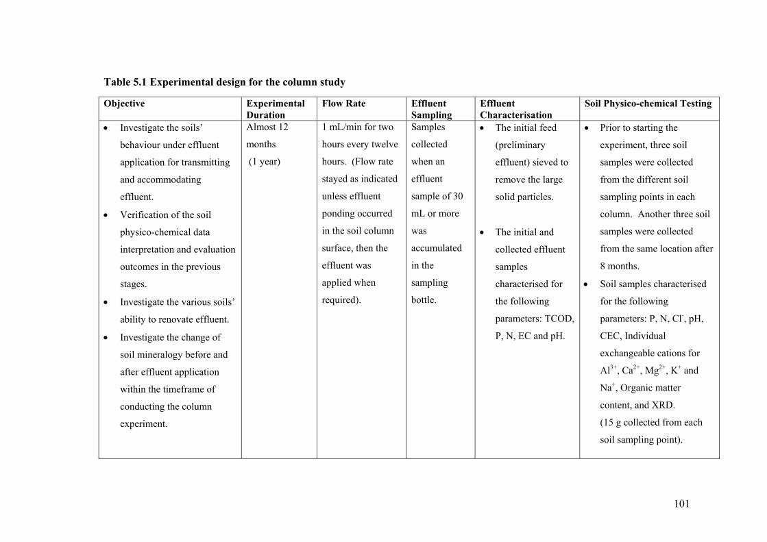
101

Table 5.1 Experimental design for the column study

Objective Experimental Duration

Flow Rate Effluent Sampling

Effluent Characterisation

Soil Physico-chemical Testing

• Investigate the soils’

behaviour under effluent

application for transmitting

and accommodating

effluent.

• Verification of the soil

physico-chemical data

interpretation and evaluation

outcomes in the previous

stages.

• Investigate the various soils’

ability to renovate effluent.

• Investigate the change of

soil mineralogy before and

after effluent application

within the timeframe of

conducting the column

experiment.

Almost 12

months

(1 year)

1 mL/min for two

hours every twelve

hours. (Flow rate

stayed as indicated

unless effluent

ponding occurred

in the soil column

surface, then the

effluent was

applied when

required).

Samples

collected

when an

effluent

sample of 30

mL or more

was

accumulated

in the

sampling

bottle.

• The initial feed

(preliminary

effluent) sieved to

remove the large

solid particles.

• The initial and

collected effluent

samples

characterised for

the following

parameters: TCOD,

P, N, EC and pH.

• Prior to starting the

experiment, three soil

samples were collected

from the different soil

sampling points in each

column. Another three soil

samples were collected

from the same location after

8 months.

• Soil samples characterised

for the following

parameters: P, N, Cl-, pH,

CEC, Individual

exchangeable cations for

Al3+, Ca2+, Mg2+, K+ and

Na+, Organic matter

content, and XRD.

(15 g collected from each

soil sampling point).

102

5.5 Laboratory Columns - Manufacture and Preparation Prior to collecting the soil cores, twelve Perspex columns of 100 mm diameter and

950 mm in length were prepared for the laboratory column experiment. Each

column was provided with three effluent sampling points. These sampling points

were located along each column side. The first sampling point was 150 mm from

the top, the second sampling point was located 510 mm from the top and the third

sampling point was located 810 mm from the top (Figure 5.1). Each sampling

point was fitted with 125 mm diameter hose tail fittings and connected with a tube

to collect the effluent into the bottles connected at the end. Along the other side

of the column, three soil sampling windows were located opposite to the effluent

sampling points. The size of each window was 50x50 mm and each window was

closed with a removable flap for future soil sampling. The columns were placed

on 25 mm thick Perspex bases, each with a central discharge point fitted with

similar hose fittings. Each set of four columns was placed on a wooden trolley as


EffluentSampling

Points

Discharging Point

Soil Sampling Windows

Soil Level

100mm

Effluent

360mm

300mm

150mm

90mm

EffluentSampling

Points

Discharging Point

Soil Sampling Windows

Soil Level

100mm

Effluent

360mm

300mm

150mm

Figure 5.1 Schematic diagram for a typical laboratory column

103

Figure 5.2 Columns placed on a trolley

5.6 Soil Cores Collection

The undisturbed soil cores were collected with adequate precautions to maintain

the structure and texture of the representative samples. These measures included:

• All cores were collected away from the roadsides to avoid any disturbed or

imported materials;

• The soil cores were collected away from watercourses; and

• All the soil cores were collected on the same day with the same size auger.

The cores were collected using the following equipment:

• Top Drive Scout III truck mounted drill rig.

104

• Hollow Auger Drill system with bits and adaptors, split spoon sampler, hand

tools and ancillary drilling equipment.

The coring was conducted by placing a 85 mm internal hollow steel tube inside a

200 mm-flite auger (Figure 5.3). The flite auger was driven hydraulically into the

soil to a depth of 900 mm. The internal hollow type auger was retracted, the split

spoon opened (Figure 5.4) and the soil core transferred to a 100 mm diameter,

2000 mm length of PVC tube to provide secure conditions for transporting the

samples to the laboratory (Figure 5.5). The flite auger was placed inside the

borehole and driven for another 900 mm, and the resultant sample core was

collected and transferred to the same PVC pipe. The undisturbed soil cores were

collected to a depth, where it could be easy to distinguish the soil horizons A and

B (Figure 5.6). All soil cores were collected to a depth of at least 1400 mm. Clear

labelling identified the collected samples, and plastic covers were placed over the

samples to protect the soil cores from any disturbances during transport to the

laboratory and prevent drying out. A complete site description for each site was

recorded. The site description included weather conditions, vegetation,

coordinates and the soil type based on the Australian Soil Classification (Isbell,

1996). The depth of the soil sampling, the topography of the site and observations

were noted on the soil core sample. In addition, the collected soil samples were

photographed in the field directly after sampling to maintain a photographic

inventory.

105

Figure 5.3 Photo presents the drilling auger with the hollow auger inside

Figure 5.4 Process of collecting the soil from the hollow auger

106

Figure 5.5 Soil core after collection

Figure 5.6 Soil core shows distinct A and B-horizons

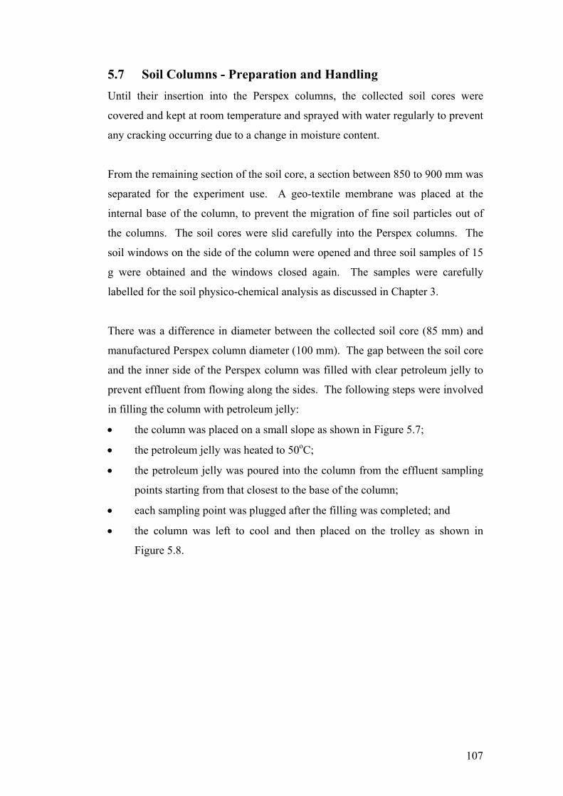
107

5.7 Soil Columns - Preparation and Handling Until their insertion into the Perspex columns, the collected soil cores were

covered and kept at room temperature and sprayed with water regularly to prevent

any cracking occurring due to a change in moisture content.

From the remaining section of the soil core, a section between 850 to 900 mm was

separated for the experiment use. A geo-textile membrane was placed at the

internal base of the column, to prevent the migration of fine soil particles out of

the columns. The soil cores were slid carefully into the Perspex columns. The

soil windows on the side of the column were opened and three soil samples of 15

g were obtained and the windows closed again. The samples were carefully

labelled for the soil physico-chemical analysis as discussed in Chapter 3.

There was a difference in diameter between the collected soil core (85 mm) and

manufactured Perspex column diameter (100 mm). The gap between the soil core

and the inner side of the Perspex column was filled with clear petroleum jelly to

prevent effluent from flowing along the sides. The following steps were involved

in filling the column with petroleum jelly:

• the column was placed on a small slope as shown in Figure 5.7;

• the petroleum jelly was heated to 50oC;

• the petroleum jelly was poured into the column from the effluent sampling

points starting from that closest to the base of the column;

• each sampling point was plugged after the filling was completed; and

• the column was left to cool and then placed on the trolley as shown in

Figure 5.8.

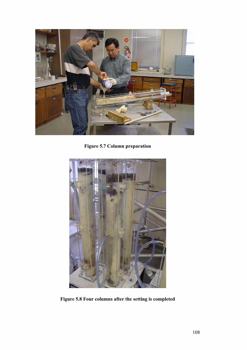
108

Figure 5.7 Column preparation

Figure 5.8 Four columns after the setting is completed

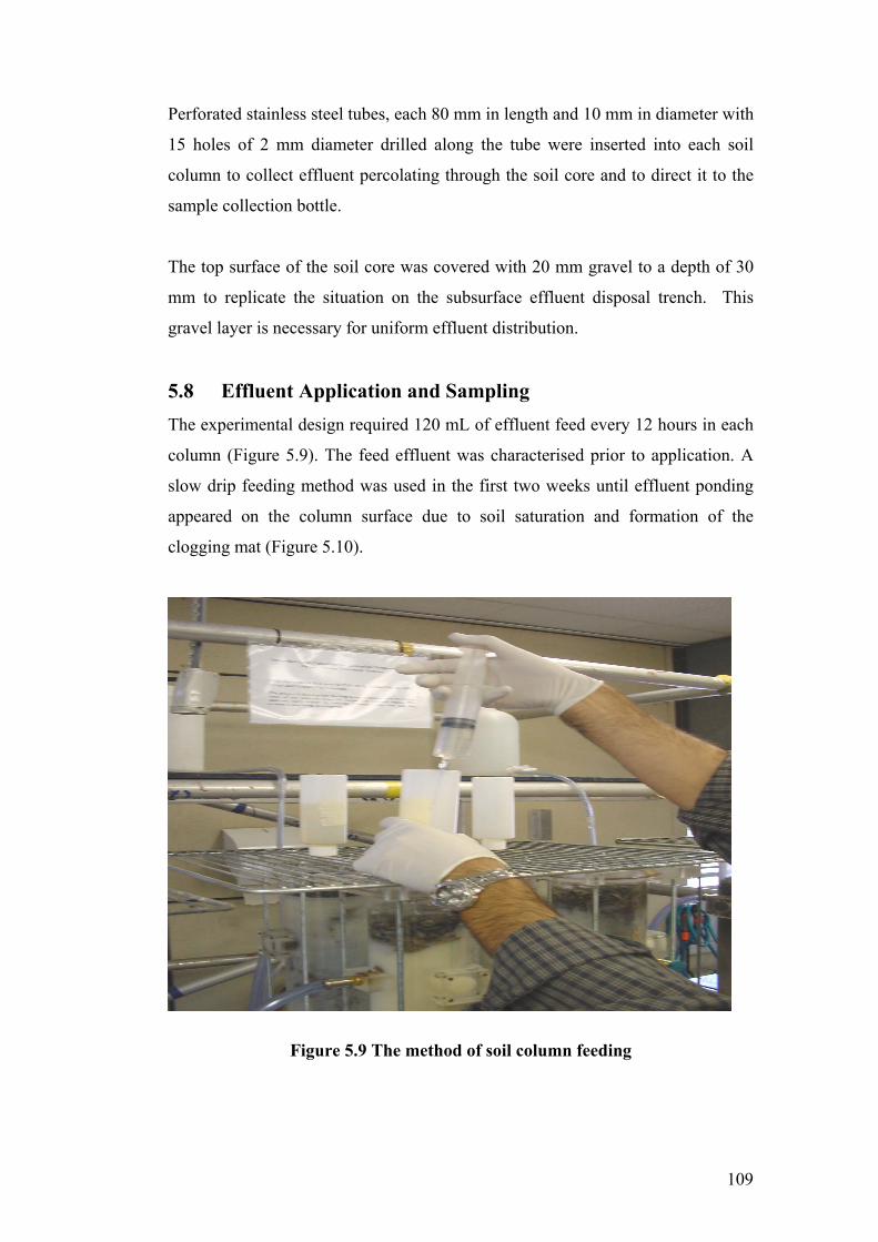
109

Perforated stainless steel tubes, each 80 mm in length and 10 mm in diameter with

15 holes of 2 mm diameter drilled along the tube were inserted into each soil

column to collect effluent percolating through the soil core and to direct it to the

sample collection bottle.

The top surface of the soil core was covered with 20 mm gravel to a depth of 30

mm to replicate the situation on the subsurface effluent disposal trench. This

gravel layer is necessary for uniform effluent distribution.

5.8 Effluent Application and Sampling The experimental design required 120 mL of effluent feed every 12 hours in each

column (Figure 5.9). The feed effluent was characterised prior to application. A

slow drip feeding method was used in the first two weeks until effluent ponding

appeared on the column surface due to soil saturation and formation of the

clogging mat (Figure 5.10).

Figure 5.9 The method of soil column feeding

110

Figure 5.10 Effluent drip-feeding

The effluent sampling points along the sides and the base of the columns were

connected to 120 mL bottles for collecting the percolating effluent (Figure 5.11).

The percolated effluent was then characterised for the parameters discussed in

Table 5.1. Figure 5.12 presents the set-up for the column experiment.

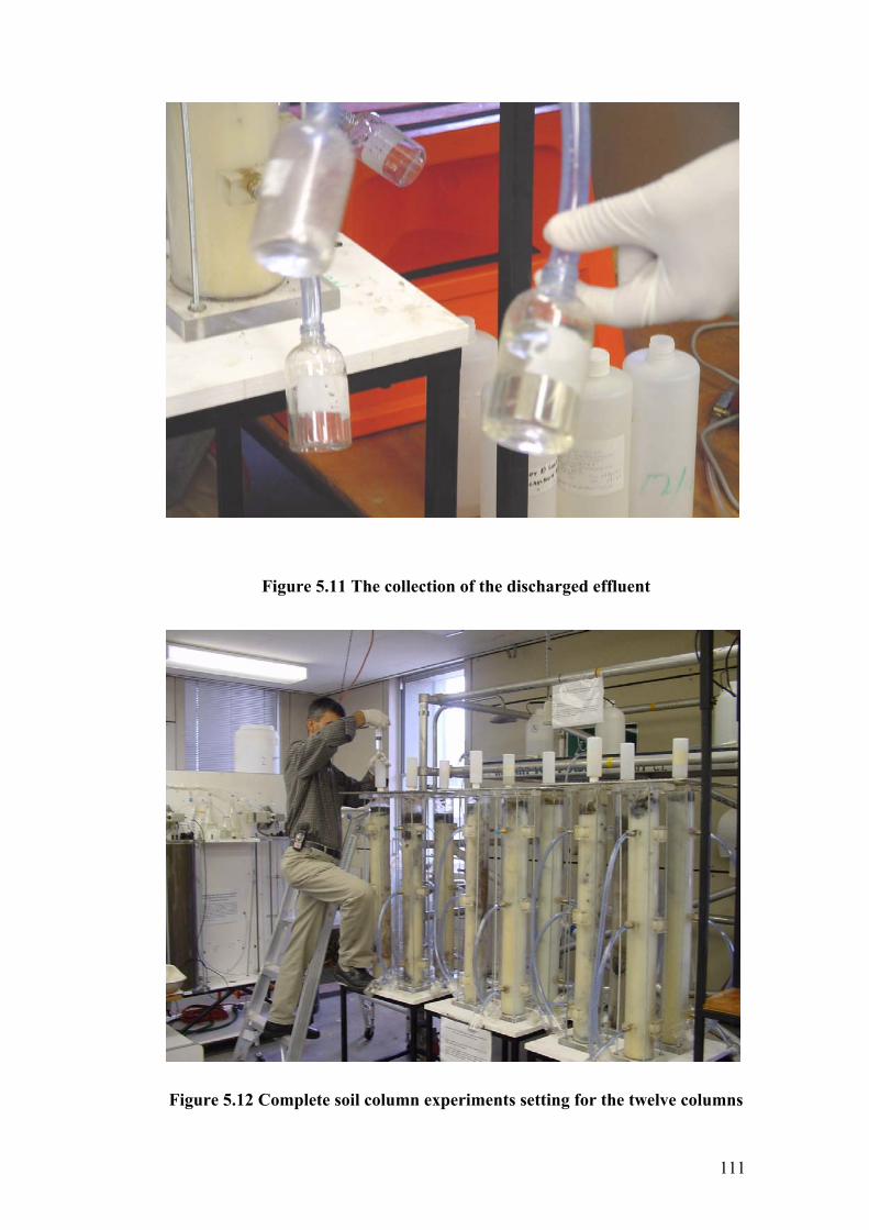
111

Figure 5.11 The collection of the discharged effluent

Figure 5.12 Complete soil column experiments setting for the twelve columns

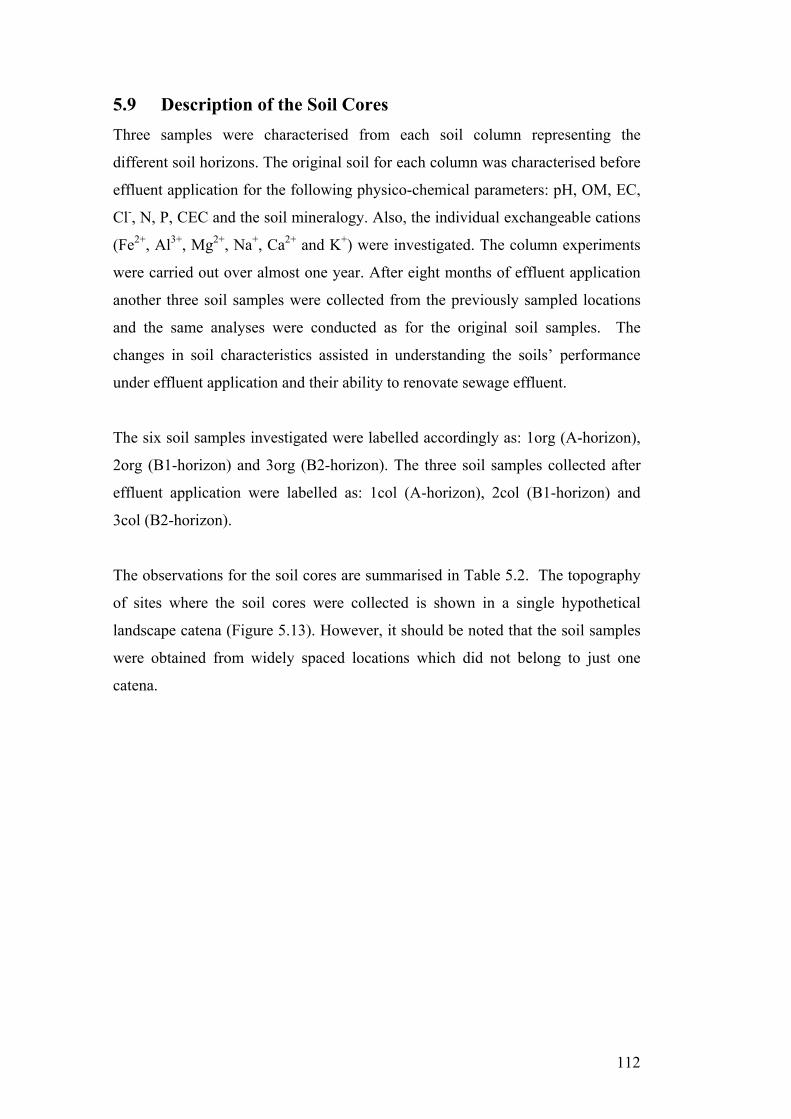
112

5.9 Description of the Soil Cores Three samples were characterised from each soil column representing the

different soil horizons. The original soil for each column was characterised before

effluent application for the following physico-chemical parameters: pH, OM, EC,

Cl-, N, P, CEC and the soil mineralogy. Also, the individual exchangeable cations

(Fe2+, Al3+, Mg2+, Na+, Ca2+ and K+) were investigated. The column experiments

were carried out over almost one year. After eight months of effluent application

another three soil samples were collected from the previously sampled locations

and the same analyses were conducted as for the original soil samples. The

changes in soil characteristics assisted in understanding the soils’ performance

under effluent application and their ability to renovate sewage effluent.

The six soil samples investigated were labelled accordingly as: 1org (A-horizon),

2org (B1-horizon) and 3org (B2-horizon). The three soil samples collected after

effluent application were labelled as: 1col (A-horizon), 2col (B1-horizon) and

3col (B2-horizon).

The observations for the soil cores are summarised in Table 5.2. The topography

of sites where the soil cores were collected is shown in a single hypothetical

landscape catena (Figure 5.13). However, it should be noted that the soil samples

were obtained from widely spaced locations which did not belong to just one

catena.

113

Table 5.2 Soil columns and field observations

Coordinates Column

Number

Soil Type

Northing Easting

Field observations

1 Yellow Kurosol 505 732 6 941 853 • A-horizon; 400-450 mm depth with high OM. • B1-horizon, 400-800 mm depth, yellow silty clay. • B2-horizon; 800-1200mm depth, yellow clay. • The topography was a high flat area followed by a deep slope. • 200mm was used from A-horizon and the rest from B-horizons. • This soil type represents the soil in Sites 7, 42 and 37.

2 Hydrosol 533 020 6 886 937 • A-horizon, around 900 mm depth, red sandy. • B1-horizon; 900- 1150 mm depth; yellowish clay. • B2-horizon; 1150- 1500 mm depth; white clay. • The core soil was obtained from a high flat area followed by a deep slope.

3 Podosol 535 691 6927 067 • A-horizon; organic rich sandy with loose structure. • B-horizon; sandy soil with high OM with no clear barrier between horizons and loose structure. • The soil core was collected from flat area with a high water table. • The soil placed in the Perspex column without petroleum jelly.

4 Black Sodosol 523 582 6 938 431 • A-horizon; 350 mm depth, sandy with clear OM. • B1-horizon; 350-700 mm depth, silty clay layer with loose structure. • B2-horizon; 700-1200 mm depth, clay layer. • The soil core was collected from the end of slope and beginning of flat area • This soil type represents the soil in Sites 33, 36, 31, 24, 43 and 44.

5 Red Dermosol 522 526 6 938 759 • A-horizon; medium brown sandy. • B1-horizon; red brown. • B2-horizon; bleached cream. • The soil core has a weak link between A and B-horizons. • The soil core has a weak structure between A and B-horizons. • This soil type represents the soil in Sites 1, 8, 11, 13, 14, 15, 29, 30, 32, 39, 5, 10, 47 and 23.

6 Brown Kurosol 521 784 6 940 756 • A-horizon; moderate brown sandy with OM. • B1-horizon; moderate brown silt clay. • B2-horizon; light brown clay. • The soil core was collected from a deep sloping area. • This soil type represents the soil in Sites 7, 42 and 37.

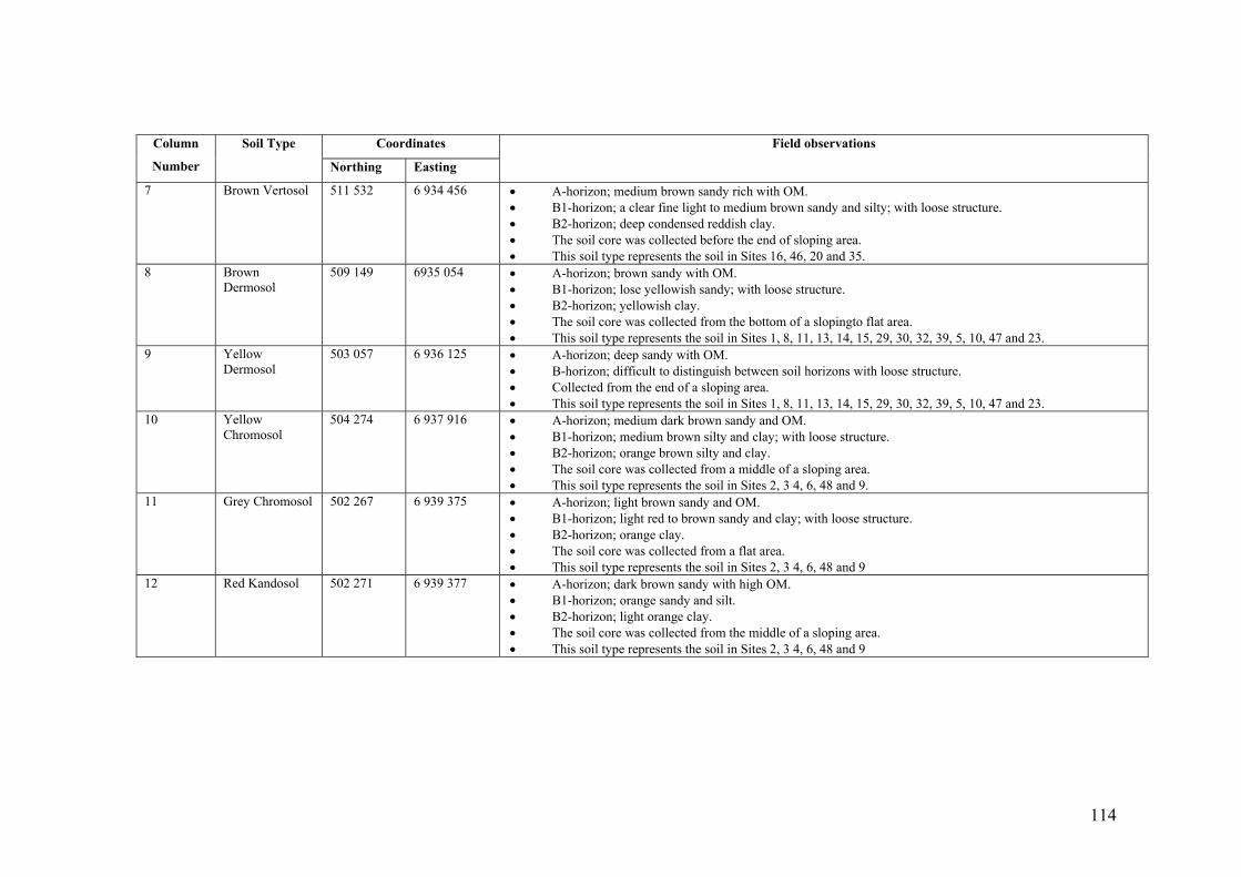
114

Coordinates Column

Number

Soil Type

Northing Easting

Field observations

7 Brown Vertosol 511 532 6 934 456 • A-horizon; medium brown sandy rich with OM. • B1-horizon; a clear fine light to medium brown sandy and silty; with loose structure. • B2-horizon; deep condensed reddish clay. • The soil core was collected before the end of sloping area. • This soil type represents the soil in Sites 16, 46, 20 and 35.

8 Brown Dermosol

509 149 6935 054 • A-horizon; brown sandy with OM. • B1-horizon; lose yellowish sandy; with loose structure. • B2-horizon; yellowish clay. • The soil core was collected from the bottom of a slopingto flat area. • This soil type represents the soil in Sites 1, 8, 11, 13, 14, 15, 29, 30, 32, 39, 5, 10, 47 and 23.

9 Yellow Dermosol

503 057 6 936 125 • A-horizon; deep sandy with OM. • B-horizon; difficult to distinguish between soil horizons with loose structure. • Collected from the end of a sloping area. • This soil type represents the soil in Sites 1, 8, 11, 13, 14, 15, 29, 30, 32, 39, 5, 10, 47 and 23.

10 Yellow Chromosol

504 274 6 937 916 • A-horizon; medium dark brown sandy and OM. • B1-horizon; medium brown silty and clay; with loose structure. • B2-horizon; orange brown silty and clay. • The soil core was collected from a middle of a sloping area. • This soil type represents the soil in Sites 2, 3 4, 6, 48 and 9.

11 Grey Chromosol 502 267 6 939 375 • A-horizon; light brown sandy and OM. • B1-horizon; light red to brown sandy and clay; with loose structure. • B2-horizon; orange clay. • The soil core was collected from a flat area. • This soil type represents the soil in Sites 2, 3 4, 6, 48 and 9

12 Red Kandosol 502 271 6 939 377 • A-horizon; dark brown sandy with high OM. • B1-horizon; orange sandy and silt. • B2-horizon; light orange clay. • The soil core was collected from the middle of a sloping area. • This soil type represents the soil in Sites 2, 3 4, 6, 48 and 9

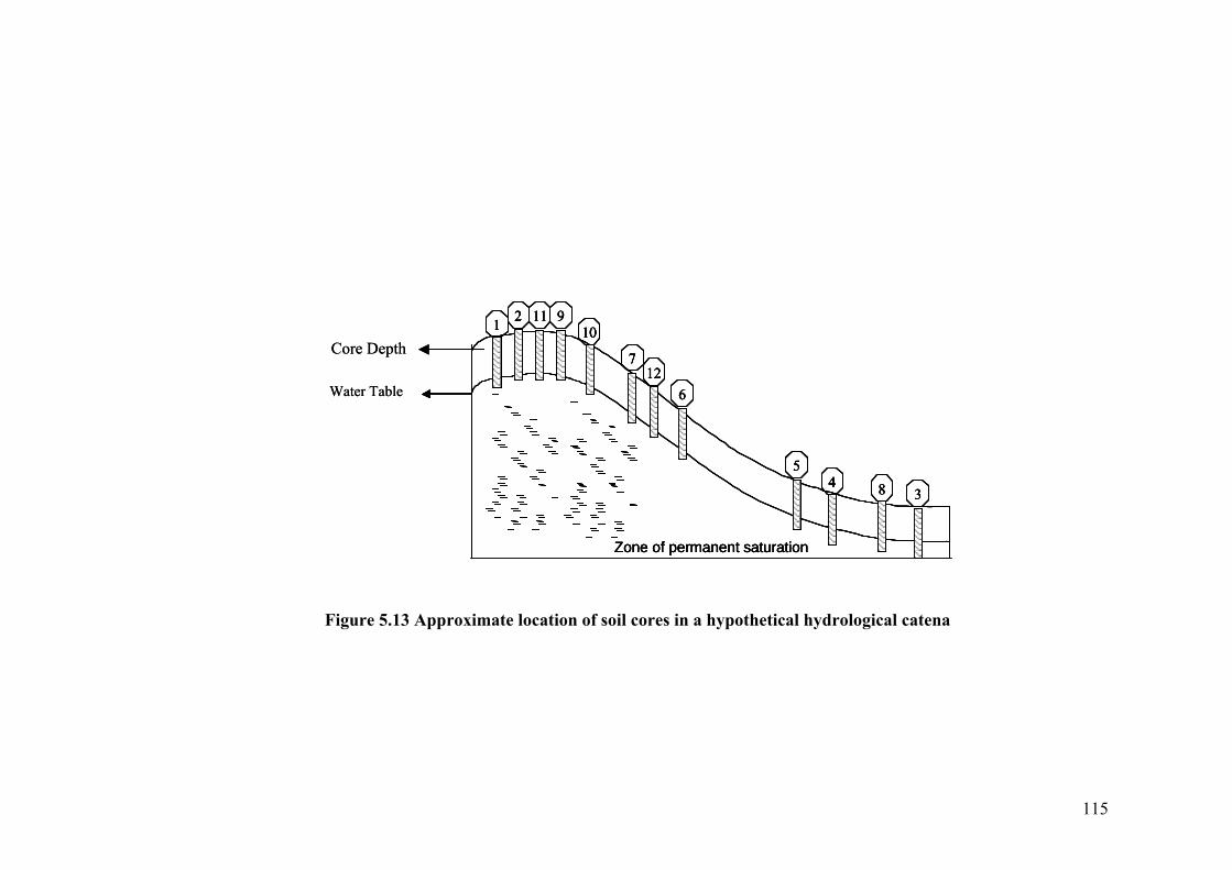
115

Figure 5.13 Approximate location of soil cores in a hypothetical hydrological catena

Zone of permanent saturation

1021

6

4 8 3

712

5

11 9


Water Table

1021

6

4 8 3

712

5

11 9

Core Depth


1021

6

4 8 3

712

5

11 9


Water Table

1021

6

4 8 3

712

5

11 9

Core Depth

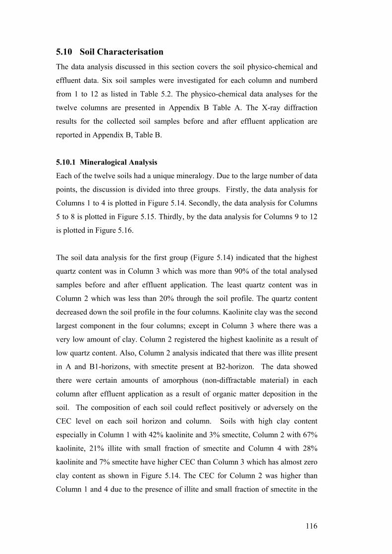
116

5.10 Soil Characterisation The data analysis discussed in this section covers the soil physico-chemical and

effluent data. Six soil samples were investigated for each column and numberd

from 1 to 12 as listed in Table 5.2. The physico-chemical data analyses for the

twelve columns are presented in Appendix B Table A. The X-ray diffraction

results for the collected soil samples before and after effluent application are

reported in Appendix B, Table B.

5.10.1 Mineralogical Analysis

Each of the twelve soils had a unique mineralogy. Due to the large number of data

points, the discussion is divided into three groups. Firstly, the data analysis for

Columns 1 to 4 is plotted in Figure 5.14. Secondly, the data analysis for Columns

5 to 8 is plotted in Figure 5.15. Thirdly, by the data analysis for Columns 9 to 12

is plotted in Figure 5.16.

The soil data analysis for the first group (Figure 5.14) indicated that the highest

quartz content was in Column 3 which was more than 90% of the total analysed

samples before and after effluent application. The least quartz content was in

Column 2 which was less than 20% through the soil profile. The quartz content

decreased down the soil profile in the four columns. Kaolinite clay was the second

largest component in the four columns; except in Column 3 where there was a

very low amount of clay. Column 2 registered the highest kaolinite as a result of

low quartz content. Also, Column 2 analysis indicated that there was illite present

in A and B1-horizons, with smectite present at B2-horizon. The data showed

there were certain amounts of amorphous (non-diffractable material) in each

column after effluent application as a result of organic matter deposition in the

soil. The composition of each soil could reflect positively or adversely on the

CEC level on each soil horizon and column. Soils with high clay content

especially in Column 1 with 42% kaolinite and 3% smectite, Column 2 with 67%

kaolinite, 21% illite with small fraction of smectite and Column 4 with 28%

kaolinite and 7% smectite have higher CEC than Column 3 which has almost zero

clay content as shown in Figure 5.14. The CEC for Column 2 was higher than

Column 1 and 4 due to the presence of illite and small fraction of smectite in the

117

Figure 5.14 Mineralogical analysis for Columns 1, 2, 3 and 4

118

soil composition which contributed slightly to CEC. In general, kaolinite is the

least active clay compared to other clays. Columns 1 and 4 have high kaolinite

content and a small fraction of smectite which improved the CEC level in these

columns. Also, smectite can form a barrier between the soil horizons preventing

the effluent contaminants leaching down to the water table. Preliminary

evaluation of these four columns based on the previous analysis indicated that the

best effluent treatment performance could be expected from Column 2 followed

by Columns 4 and 1 and the worst performance expected from Column 3 as a

result of the soil minerlogy. This soil performance evaluation was to be updated

based on the soils’ performance under effluent application.

The soil data analysis for the second group showed that the quartz was the major

mineral in these four columns. The highest quartz content of 87% was in Column

8 and the lowest, 61% was in Column 6 as shown in Figure 5.15. As for the first

group, the quartz content decreased down the soil profile in the four columns. The

second highest fraction in all columns was kaolinite clay and overall the highest

of 43% was in Column 7. Illite was present in small fractions in all columns

except in Column 7 which had higher kaolinite content than the other columns.

None of the investigated four columns reported smecitite presence. The physico-

chemical data analysis showed low CEC level in Columns 5 (10 meq/100g), 6 (5

meq/100g) and 8 (9 meq/100g), indicating that the small amount of illite in the

composition did not affect the CEC significantly. Preliminary evaluation of the

group indicated that the best performance could be expected from Column 7 (31

meq/100g), followed by 8, 6 and 5. This is due to the high clay content at B-

horizon in Column 7.

The soil data analysis for the third group showed that quartz was the major

mineral in these four columns similar to the previously discussed two groups.

Kaolinite was the second most common mineral in Columns 9 with 3%, 10 with

23% and 11 with 4% associated with a second clay mineral, illite, in Column 12

with 27%. Also, there was a small fraction of illite at B2-horizons in Columns 9

with 7% and 11 with 4% as shown in Figure 5.16. The presence of illite in these

columns reflected slightly on the available soil CEC level. In the

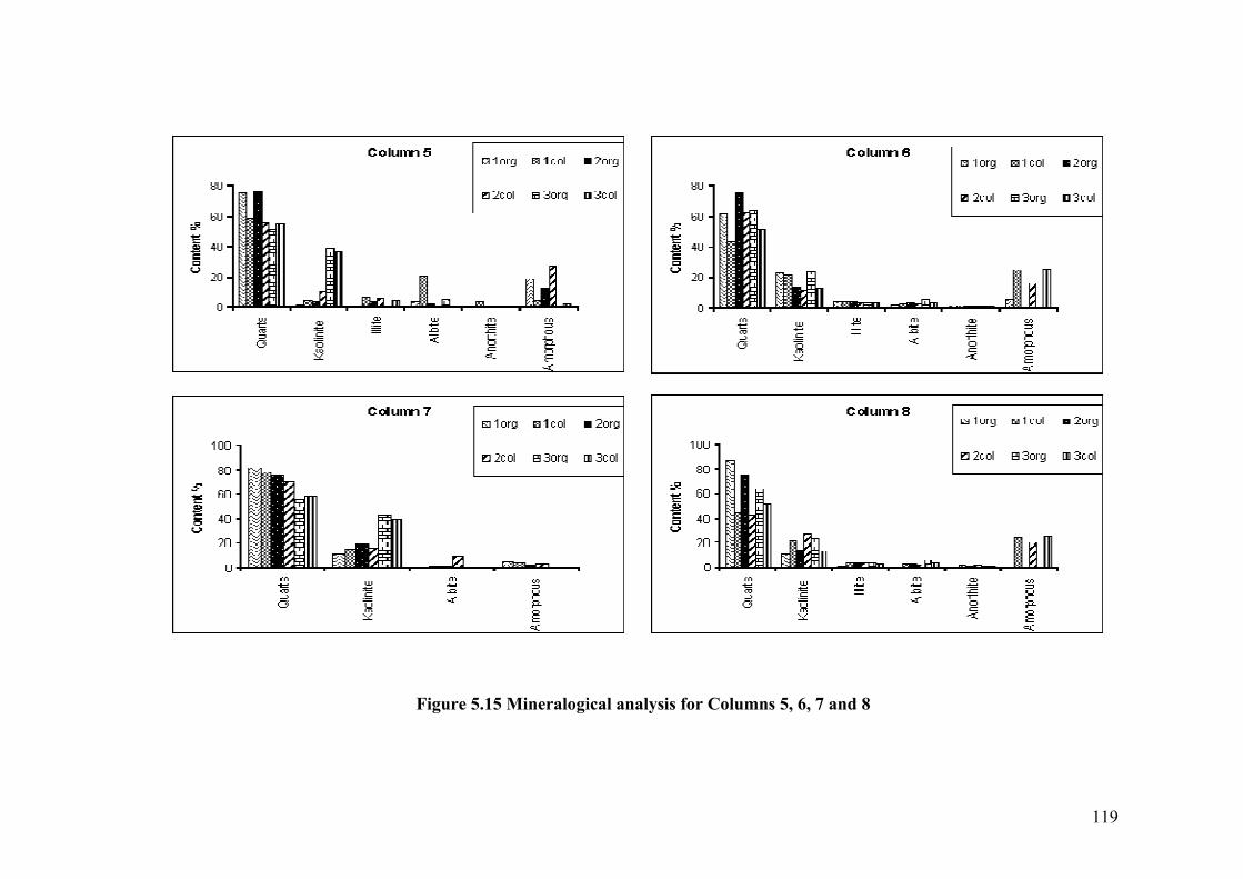
119


120


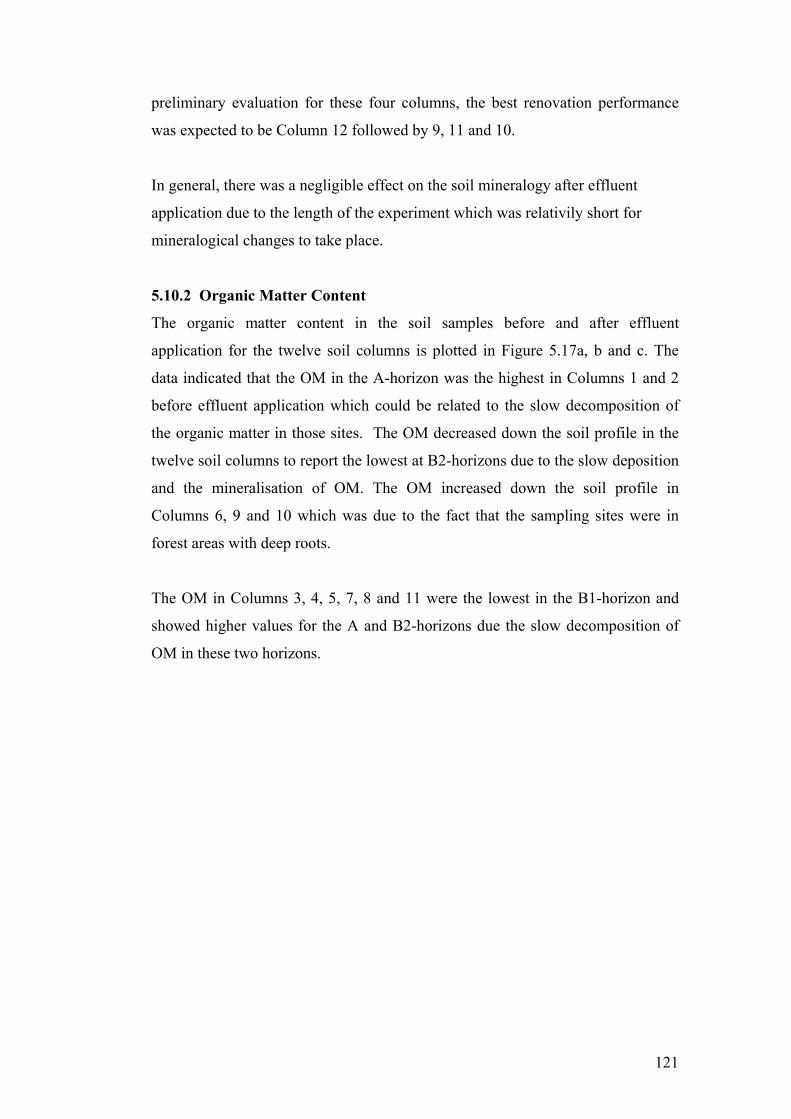
121

preliminary evaluation for these four columns, the best renovation performance

was expected to be Column 12 followed by 9, 11 and 10.

In general, there was a negligible effect on the soil mineralogy after effluent

application due to the length of the experiment which was relativily short for

mineralogical changes to take place.

5.10.2 Organic Matter Content

The organic matter content in the soil samples before and after effluent

application for the twelve soil columns is plotted in Figure 5.17a, b and c. The

data indicated that the OM in the A-horizon was the highest in Columns 1 and 2

before effluent application which could be related to the slow decomposition of

the organic matter in those sites. The OM decreased down the soil profile in the

twelve soil columns to report the lowest at B2-horizons due to the slow deposition

and the mineralisation of OM. The OM increased down the soil profile in

Columns 6, 9 and 10 which was due to the fact that the sampling sites were in

forest areas with deep roots.

The OM in Columns 3, 4, 5, 7, 8 and 11 were the lowest in the B1-horizon and

showed higher values for the A and B2-horizons due the slow decomposition of

OM in these two horizons.

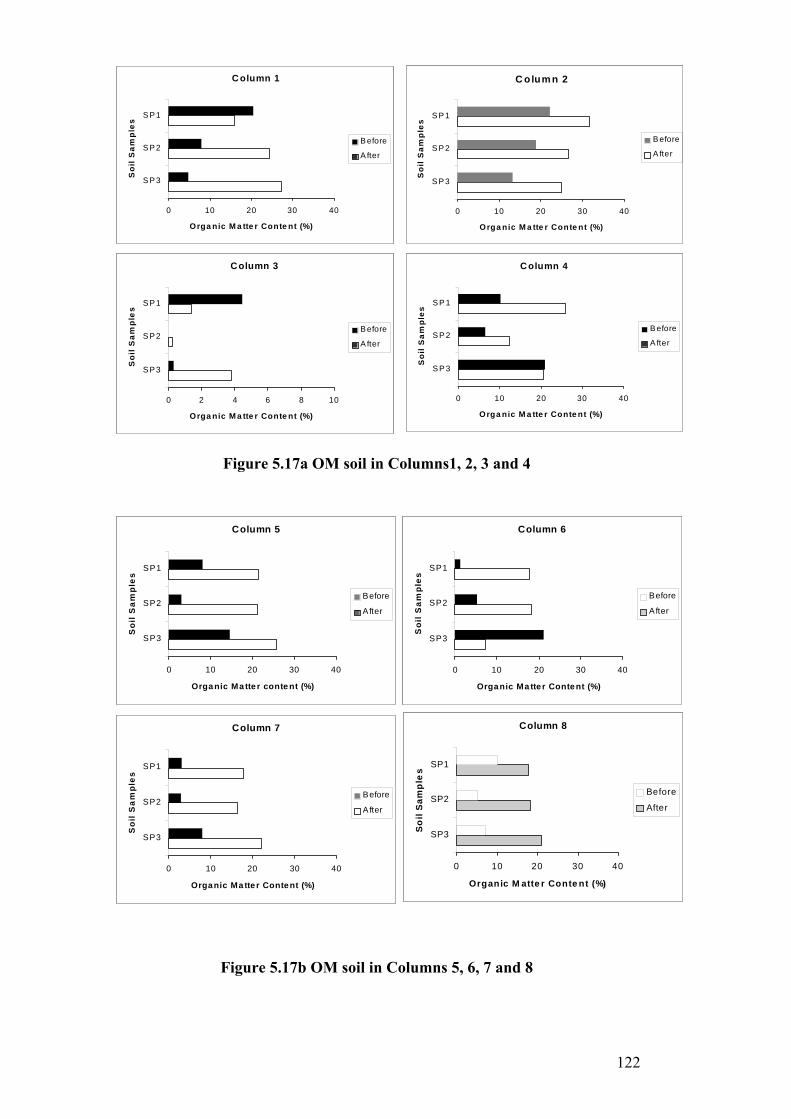
122

Figure 5.17a OM soil in Columns1, 2, 3 and 4

Figure 5.17b OM soil in Columns 5, 6, 7 and 8

Column 5

0 10 20 30 40

SP3

SP2

SP1

Soi

l Sam

ples

Organic Ma tter content (%)

Before

After

Column 6

0 10 20 30 40

SP3

SP2

SP1

Soi

l Sam

ples

Organic Ma tte r Conte nt (%)

Before

After

Column 7

0 10 20 30 40

SP3

SP2

SP1

Soi

l Sam

ples

Organic Ma tte r Content (%)

Before

After

Column 8

0 10 20 30 40

SP3

SP2

SP1

So

il S

amp

les

Organic M atte r Conte nt (%)

Before

After

Column 5

0 10 20 30 40

SP3

SP2

SP1

Soi

l Sam

ples

Orga nic Ma tte r conte nt (%)

Before

After

Column 6

0 10 20 30 40

SP3

SP2

SP1

Soi

l Sam

ples

Organic Ma tte r Conte nt (%)

Before

After

Column 7

0 10 20 30 40

SP3

SP2

SP1

Soi

l Sam

ples

Organic Ma tte r Content (%)

Before

After

Column 8

0 10 20 30 40

SP3

SP2

SP1

So

il S

amp

les


Before

After

C olum n 2

0 10 20 30 40

S P 3

S P 2

S P 1

Soi

l S

ampl

es

O rga nic M a tte r Conte nt (%)

B efore

A fter

C olumn 1

0 10 20 30 40

S P 3

S P 2

S P 1

Soi

l Sam

ples


B efore

A fter

Column 3

0 2 4 6 8 10

SP3

SP2

SP1

So

il S

ampl

es


Before

A fter

C olumn 4

0 10 20 30 40

S P 3

S P 2

S P 1

Soi

l Sam

ples


B efore

A fter

C olum n 2

0 10 20 30 40

S P 3

S P 2

S P 1

Soi

l Sam

ples


B efore

A fter

C olumn 1

0 10 20 30 40

S P 3

S P 2

S P 1

Soi

l Sam

ples


B efore

A fter

Column 3

0 2 4 6 8 10

SP3

SP2

SP1

So

il S

ampl

es


Before

A fter

C olumn 4

0 10 20 30 40

S P 3

S P 2

S P 1

Soi

l Sam

ples


B efore

A fter

123

Effluent application increased the OM in the soil layers based on the level of

biochemical activity in the soil. For instance, the OM in A-horizon for all columns

increased except in Columns 1 and 3 where it decreased. In Column 1 this is

related to the high decomposition rate as a result of the suitable pH condition for

biological activity to take place at the A-horizon in this soil. The soil pH in

Column 1 was 6.09, the highest pH’s of all columns at A-horizon.. The case in

Column 3 is different. This column is a sandy soil with large pore sizes. The large

pore sizes allow the OM carried by the effluent to travel down the soil profile.

Figure 5.17c OM soil in Columns 9, 10, 11 and 12

The OM in the twelve columns increased at B1-horizon after effluent application.

This could be attributed to the slow biological activity and the high deposition rate

in this horizon. OM increased at B2-horizons in most columns except in Columns

4, 6 and 12. In the case of Column 4, the OM stayed at almost the same level due

to the presence of smectite clay which formed a barrier preventing the dissolved

OM from percolating through this layer as a result of shrink/swell mechanisms of

the smectite clay. The case in Columns 6 and 12 is different. In these columns the

Column 9

0 10 20 30 40

SP3

SP2

SP1

So

il S

amp

les


Before

After

Column 10

0 10 20 30 40

SP3

SP2

SP1

So

il S

amp

les


Before

After

Column 11

0 10 20 30 40

SP3

SP2

SP1

So

il S

amp

les


Before

After

Column 12

0 10 20 30 40

SP3

SP2

SP1

So

il S

amp

les


Before

After

Column 9

0 10 20 30 40

SP3

SP2

SP1

So

il S

amp

les


Before

After

Column 10

0 10 20 30 40

SP3

SP2

SP1

So

il S

amp

les


Before

After

Column 11

0 10 20 30 40

SP3

SP2

SP1

So

il S

amp

les


Before

After

Column 12

0 10 20 30 40

SP3

SP2

SP1

So

il S

amp

les


Before

After

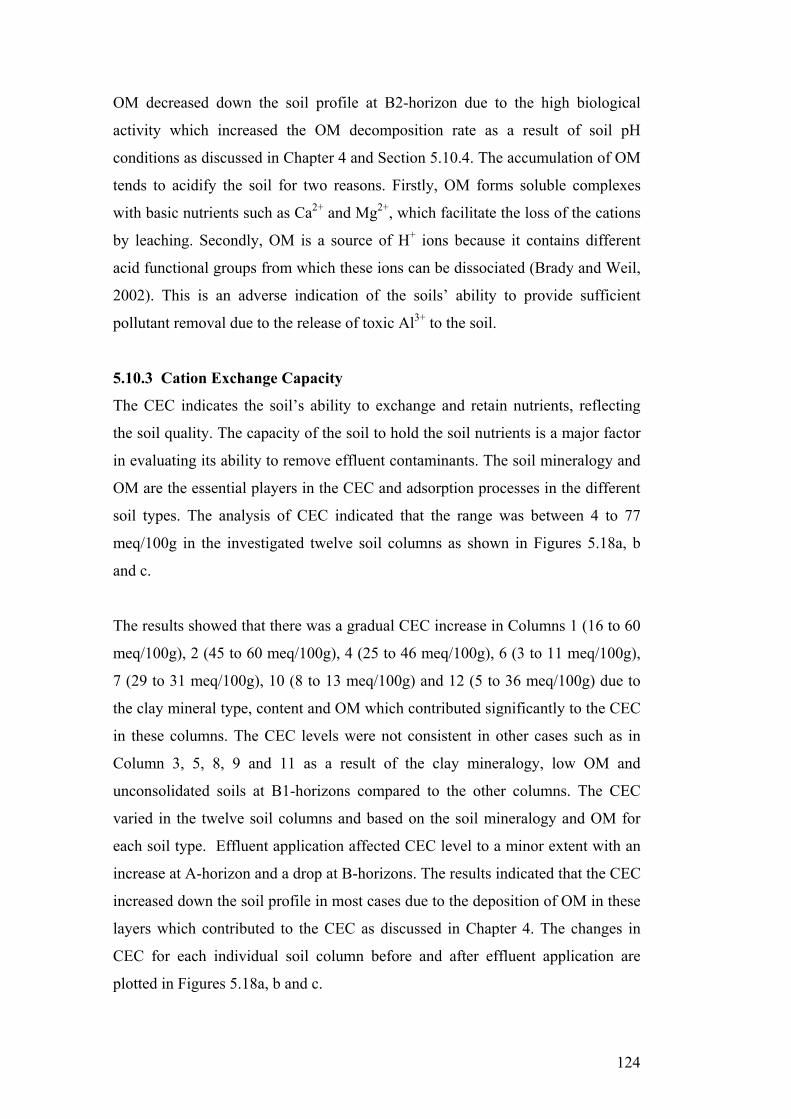
124

OM decreased down the soil profile at B2-horizon due to the high biological

activity which increased the OM decomposition rate as a result of soil pH

conditions as discussed in Chapter 4 and Section 5.10.4. The accumulation of OM

tends to acidify the soil for two reasons. Firstly, OM forms soluble complexes

with basic nutrients such as Ca2+ and Mg2+, which facilitate the loss of the cations

by leaching. Secondly, OM is a source of H+ ions because it contains different

acid functional groups from which these ions can be dissociated (Brady and Weil,

2002). This is an adverse indication of the soils’ ability to provide sufficient

pollutant removal due to the release of toxic Al3+ to the soil.

5.10.3 Cation Exchange Capacity

The CEC indicates the soil’s ability to exchange and retain nutrients, reflecting

the soil quality. The capacity of the soil to hold the soil nutrients is a major factor

in evaluating its ability to remove effluent contaminants. The soil mineralogy and

OM are the essential players in the CEC and adsorption processes in the different

soil types. The analysis of CEC indicated that the range was between 4 to 77

meq/100g in the investigated twelve soil columns as shown in Figures 5.18a, b

and c.

The results showed that there was a gradual CEC increase in Columns 1 (16 to 60

meq/100g), 2 (45 to 60 meq/100g), 4 (25 to 46 meq/100g), 6 (3 to 11 meq/100g),

7 (29 to 31 meq/100g), 10 (8 to 13 meq/100g) and 12 (5 to 36 meq/100g) due to

the clay mineral type, content and OM which contributed significantly to the CEC

in these columns. The CEC levels were not consistent in other cases such as in

Column 3, 5, 8, 9 and 11 as a result of the clay mineralogy, low OM and

unconsolidated soils at B1-horizons compared to the other columns. The CEC

varied in the twelve soil columns and based on the soil mineralogy and OM for

each soil type. Effluent application affected CEC level to a minor extent with an

increase at A-horizon and a drop at B-horizons. The results indicated that the CEC

increased down the soil profile in most cases due to the deposition of OM in these

layers which contributed to the CEC as discussed in Chapter 4. The changes in

CEC for each individual soil column before and after effluent application are

plotted in Figures 5.18a, b and c.

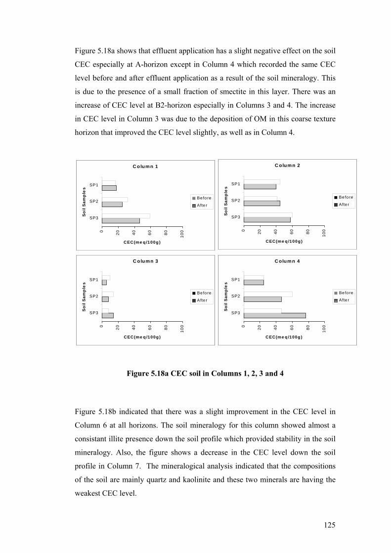
125

Figure 5.18a shows that effluent application has a slight negative effect on the soil

CEC especially at A-horizon except in Column 4 which recorded the same CEC

level before and after effluent application as a result of the soil mineralogy. This

is due to the presence of a small fraction of smectite in this layer. There was an

increase of CEC level at B2-horizon especially in Columns 3 and 4. The increase

in CEC level in Column 3 was due to the deposition of OM in this coarse texture

horizon that improved the CEC level slightly, as well as in Column 4.

Figure 5.18a CEC soil in Columns 1, 2, 3 and 4

Figure 5.18b indicated that there was a slight improvement in the CEC level in

Column 6 at all horizons. The soil mineralogy for this column showed almost a

consistant illite presence down the soil profile which provided stability in the soil

mineralogy. Also, the figure shows a decrease in the CEC level down the soil

profile in Column 7. The mineralogical analysis indicated that the compositions

of the soil are mainly quartz and kaolinite and these two minerals are having the

weakest CEC level.

C olumn 1

0 20 40 60 80 100

SP3

SP2

SP1

So

il S

amp

les

CEC(me q /100g )

Befo re

After

C olum n 2

0 20 40 60 80 100

SP3

SP2

SP1

So

il S

amp

les

CEC(me q /100g )

Before

Afte r

C olum n 3

0 20 40 60 80 100

SP3

SP2

SP1

So

il S

amp

les

CEC(me q /100g )

Before

Afte r

C olum n 4

0 20 40 60 80 100

SP3

SP2

SP1

So

il S

amp

les

CEC(me q /100g )

Before

Afte r

C olum n 1

0 20 40 60 80 100

SP3

SP2

SP1

So

il S

amp

les

CEC(me q /100g )

Befo re

Afte r

C olum n 2

0 20 40 60 80 100

SP3

SP2

SP1

So

il S

amp

les

CEC(me q /100g )

Before

Afte r

C olum n 3

0 20 40 60 80 100

SP3

SP2

SP1

So

il S

amp

les

CEC(me q /100g )

Before

Afte r

C olum n 4

0 20 40 60 80 100

SP3

SP2

SP1

So

il S

amp

les

CEC(me q /100g )

Before

Afte r

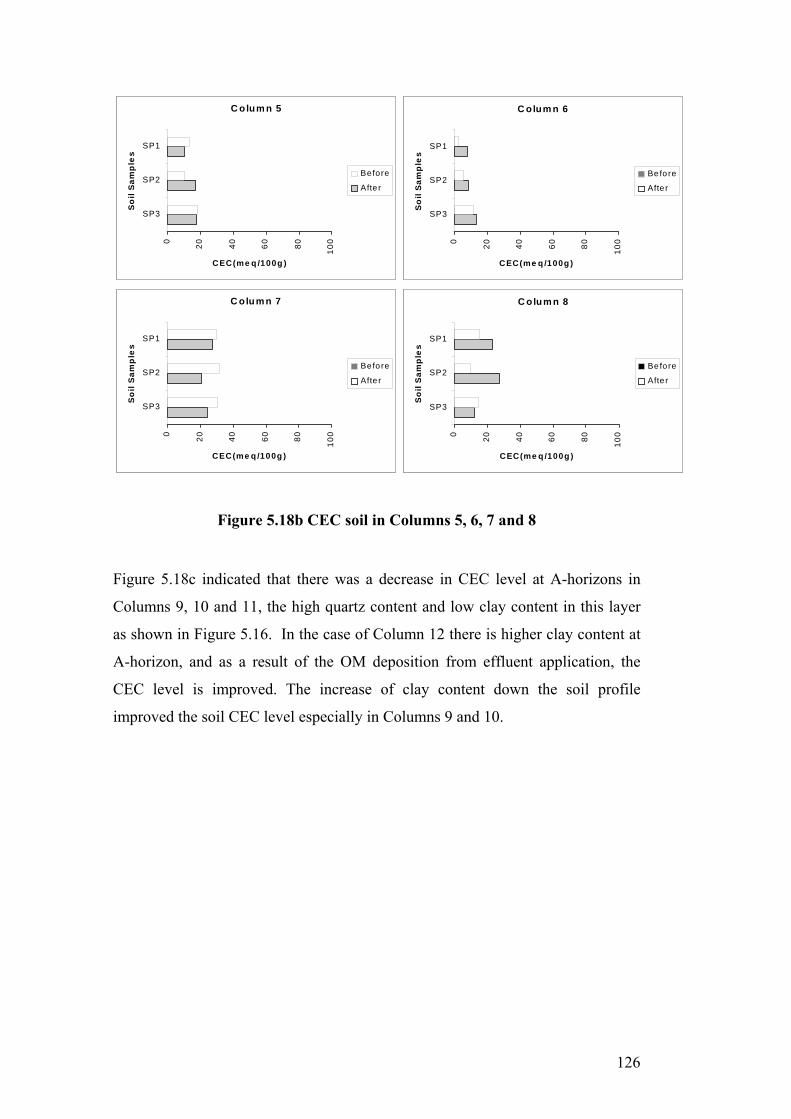
126

Figure 5.18b CEC soil in Columns 5, 6, 7 and 8 Figure 5.18c indicated that there was a decrease in CEC level at A-horizons in

Columns 9, 10 and 11, the high quartz content and low clay content in this layer

as shown in Figure 5.16. In the case of Column 12 there is higher clay content at

A-horizon, and as a result of the OM deposition from effluent application, the

CEC level is improved. The increase of clay content down the soil profile

improved the soil CEC level especially in Columns 9 and 10.

C olum n 5

0 20 40 60 80 100

SP3

SP2

SP1

So

il S

amp

les

CEC(me q /100g )

Before

Afte r

C olum n 6

0 20 40 60 80 100

SP3

SP2

SP1

So

il S

amp

les

CEC(me q /100g )

Before

After

C olum n 7

0 20 40 60 80 100

SP3

SP2

SP1

So

il S

amp

les

CEC(me q /100g )

Before

Afte r

C olum n 8

0 20 40 60 80 100

SP3

SP2

SP1

So

il S

amp

les

CEC(me q /100g )

Before

After

C olum n 5

0 20 40 60 80 100

SP3

SP2

SP1

So

il S

amp

les

CEC(me q /100g )

Before

Afte r

C olum n 6

0 20 40 60 80 100

SP3

SP2

SP1

So

il S

amp

les

CEC(me q /100g )

Befo re

After

C olum n 7

0 20 40 60 80 100

SP3

SP2

SP1

So

il S

amp

les

CEC(me q /100g )

Befo re

Afte r

C olum n 8

0 20 40 60 80 100

SP3

SP2

SP1

So

il S

amp

les

CEC(me q /100g )

Before

After

127

Figure 5.18c CEC soil in Columns 9, 10, 11 and 12 5.10.4 pH

The pH values for the twelve soil columns in the original soil samples were below

6.5. Lower pH values (<5.5) were reported in the B-horizons compared to the pH

values in the A-horizons for most columns (Figure 5.19a, b and c). These soils

exhibit an acid reaction throughout the profile, which could become a problem

especially when the pH drops below 5.5. The low pH (< 5.5) could lead to less

microbial activity as a result of release of aluminium to form a toxic medium for

microorganisms. Also, if the acidic soil has low clay or OM, the problem becomes

greater because the soil has lower resistance for pH change (Brady, 1984).

The twelve soils were classified according to their acidity at A-horizon. Columns

8 and 6 are extremely acidic (pH< 4.5). Columns 2, 4 and 10 are very strongly

acidic (pH= 4.5-5.0). Columns 3 and 9 are strongly acidic (pH= 5.1-5.5).

Columns 5, 7 and 12 are moderately acidic (pH= 5.6-6). Columns 1 and 11 are

slightly acid (pH= 6.1-6.5). The lowest pH values was reported in Column 8 and

the highest pH value was reported in Column 11. The low pH in Column 8 could

C olumn 9

0 20 40 60 80 100

SP3

SP2

SP1

So

il S

amp

les

CEC(me q /100g )

Before

After

C olumn 10

0 20 40 60 80 100

SP3

SP2

SP1

So

il S

amp

les

CEC(me q /100g )

Before

Afte r

C olum n 11

0 20 40 60 80 100

SP3

SP2

SP1

So

il S

amp

les

CEC(me q /100g )

Before

After

C olum n 12

0 20 40 60 80 100

SP3

SP2

SP1

So

il S

amp

les

CEC(me q /100g)

Before

After

C olum n 9

0 20 40 60 80 100

SP3

SP2

SP1

So

il S

amp

les

CEC(me q /100g )

Before

After

C olumn 10

0 20 40 60 80 100

SP3

SP2

SP1

So

il S

amp

les

CEC(me q /100g )

Before

Afte r

C olum n 11

0 20 40 60 80 100

SP3

SP2

SP1

So

il S

amp

les

CEC(me q /100g )

Before

After

C olum n 12

0 20 40 60 80 100

SP3

SP2

SP1

So

il S

amp

les

CEC(me q /100g)

Before

After

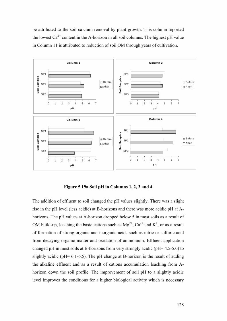
128

be attributed to the soil calcium removal by plant growth. This column reported

the lowest Ca2+ content in the A-horizon in all soil columns. The highest pH value

in Column 11 is attributed to reduction of soil OM through years of cultivation.

Figure 5.19a Soil pH in Columns 1, 2, 3 and 4

The addition of effluent to soil changed the pH values slightly. There was a slight

rise in the pH level (less acidic) at B-horizons and there was more acidic pH at A-

horizons. The pH values at A-horizon dropped below 5 in most soils as a result of

OM build-up, leaching the basic cations such as Mg2+, Ca2+ and K+, or as a result

of formation of strong organic and inorganic acids such as nitric or sulfuric acid

from decaying organic matter and oxidation of ammonium. Effluent application

changed pH in most soils at B-horizons from very strongly acidic (pH= 4.5-5.0) to

slightly acidic (pH= 6.1-6.5). The pH change at B-horizon is the result of adding

the alkaline effluent and as a result of cations accumulation leaching from A-

horizon down the soil profile. The improvement of soil pH to a slightly acidic

level improves the conditions for a higher biological activity which is necessary

Column 1

0 1 2 3 4 5 6 7

SP3

SP2

SP1

So

il S

amp

les

pH

Before

After

Column 2

0 1 2 3 4 5 6 7

SP3

SP2

SP1

So

il S

amp

les

pH

Before

After

Column 3

0 1 2 3 4 5 6 7

SP3

SP2

SP1

So

il S

amp

les

pH

Before

After

Column 4

0 1 2 3 4 5 6 7

SP3

SP2

SP1

So

il S

amp

les

pH

Before

After

Column 1

0 1 2 3 4 5 6 7

SP3

SP2

SP1

So

il S

amp

les

pH

Before

After

Column 2

0 1 2 3 4 5 6 7

SP3

SP2

SP1

So

il S

amp

les

pH

Before

After

Column 3

0 1 2 3 4 5 6 7

SP3

SP2

SP1

So

il S

amp

les

pH

Before

After

Column 4

0 1 2 3 4 5 6 7

SP3

SP2

SP1

So

il S

amp

les

pH

Before

After

129

for effluent renovation. This means that effluent application affected the soil

acidity positively, which will further improve its ability to renovate effluent.

Figure 5.19b Soil pH in Columns 5, 6, 7 and 8

Column 5

0 1 2 3 4 5 6 7

SP3

SP2

SP1

So

il S

amp

les

pH

Before

After

Column 6

0 1 2 3 4 5 6 7

SP3

SP2

SP1

So

il S

amp

les

pH

Before

After

Column 7

0 1 2 3 4 5 6 7

SP3

SP2

SP1

So

il S

amp

les

pH

Before

After

Column 8

0 1 2 3 4 5 6 7

SP3

SP2

SP1S

oil

Sam

ple

s

pH

Before

After

Column 5

0 1 2 3 4 5 6 7

SP3

SP2

SP1

So

il S

amp

les

pH

Before

After

Column 6

0 1 2 3 4 5 6 7

SP3

SP2

SP1

So

il S

amp

les

pH

Before

After

Column 7

0 1 2 3 4 5 6 7

SP3

SP2

SP1

So

il S

amp

les

pH

Before

After

Column 8

0 1 2 3 4 5 6 7

SP3

SP2

SP1S

oil

Sam

ple

s

pH

Before

After

130

Figure 5.19c Soil pH in Columns 9, 10, 11 and 12

5.10.5 Electrical Conductivity

Another important physico-chemical parameter investigated was EC. EC is a

measure of the concentration of the soluble salts in the soil, which has the ability

to leach down the soil profile or into the plant roots. The soil physico-chemical

analysis indicated that the EC level in the original soils at the A-horizons were

high and decreased down the soil profile such as in Columns 1, 2, 4, 5, 6, 7 and 10

(Figure 5.20a, b and c). The mineralogy of these soils include almost 70% quartz,

and 10% kaolinite and others at the A-horizon. The high clay content could be the

reason for the high EC at the A-horizon. The clay fraction reduced the soluble

salts from leaching down the soil profile. A high EC level was recorded at B1-

horizon in Columns 3, 8, 9 and 12. The accumulation of soluble salts at the B1-

horizon is attributed to the soil mineralogy for Columns 3 and 9 which indicated

that over 90% of soil composition at this layer is quartz which allowed the soluble

salts to accumulate due to the large pore sizes. In the case of Column 8 the soil is

unconsolidated at the B1-horizon which allowed the soluble salts to accumulate

(Figure 5.20b). Column 12 was collected from the bottom of a sloping area, where

Column 9

0 1 2 3 4 5 6 7

SP3

SP2

SP1

So

il S

amp

les

pH

Before

After

Column 10

0 1 2 3 4 5 6 7

SP3

SP2

SP1

So

il S

amp

les

pH

Before

After

Column 11

0 1 2 3 4 5 6 7

SP3

SP2

SP1

So

il S

amp

les

pH

Before

After

Column 12

0 1 2 3 4 5 6 7

SP3

SP2

SP1

So

il S

amp

les

pH

Before

After

Column 9

0 1 2 3 4 5 6 7

SP3

SP2

SP1

So

il S

amp

les

pH

Before

After

Column 10

0 1 2 3 4 5 6 7

SP3

SP2

SP1

So

il S

amp

les

pH

Before

After

Column 11

0 1 2 3 4 5 6 7

SP3

SP2

SP1

So

il S

amp

les

pH

Before

After

Column 12

0 1 2 3 4 5 6 7

SP3

SP2

SP1

So

il S

amp

les

pH

Before

After

131

most of the water run-off accumulates and carries away the soluble salts. Finally,

the EC value in Column 11 is the highest at the B2-horizon (Figure 5.20c). This

soil mineralogy indicated that this horizon has low clay content which allowed the

soluble salts to accumulate.

Effluent application highly increased the EC content in soil columns except for

Column 6 where there was an increase at B1-horizon and a decrease at B2-

horizon The changes of EC levels for each soil column before and after effluent

application are presented in Figure 5.20a, b and c.

Figure 5.20a EC level in Columns 1, 2, 3 and 4

Column 1

0

200

400

600

800

1000

1200

1400

1600

1800

SP3

SP2

SP1

So

il S

amp

les

EC (µS/cm)

Before

After

Column 2

0

200

400

600

800

1000

1200

1400

1600

1800

SP3

SP2

SP1S

oil

Sam

ple

s

EC (µS/cm)

Before

After

Column 3

0

400

800

1200

1600

2000

SP3

SP2

SP1

So

il S

amp

les

EC (µS/cm)

Before

After

Column 4

0

400

800

1200

1600

2000

SP3

SP2

SP1

So

il S

amp

les

EC (µS/cm)

Before

After

Column 1

0

200

400

600

800

1000

1200

1400

1600

1800

SP3

SP2

SP1

So

il S

amp

les

EC (µS/cm)

Before

After

Column 2

0

200

400

600

800

1000

1200

1400

1600

1800

SP3

SP2

SP1S

oil

Sam

ple

s

EC (µS/cm)

Before

After

Column 3

0

400

800

1200

1600

2000

SP3

SP2

SP1

So

il S

amp

les

EC (µS/cm)

Before

After

Column 4

0

400

800

1200

1600

2000

SP3

SP2

SP1

So

il S

amp

les

EC (µS/cm)

Before

After

132

Figure 5.20b EC level in Columns 5, 6, 7 and 8

Figure 5.20c EC level in Columns 9, 10, 11 and 12

Column 5

0

400

800

1200

1600

2000

SP3

SP2

SP1

So

il S

amp

les

EC (µS/cm)

Before

After

Column 6

0

400

800

1200

1600

2000

SP3

SP2

SP1

So

il S

amp

les

EC (µS/cm)

Before

After

Column 7

0

400

800

1200

1600

2000

SP3

SP2

SP1

So

il S

amp

les

EC (µS/cm)

Before

After

Column 8

0

400

800

1200

1600

2000

SP3

SP2

SP1

So

il S

amp

les

EC (µS/cm)

Before

After

Column 5

0

400

800

1200

1600

2000

SP3

SP2

SP1

So

il S

amp

les

EC (µS/cm)

Before

After

Column 6

0

400

800

1200

1600

2000

SP3

SP2

SP1

So

il S

amp

les

EC (µS/cm)

Before

After

Column 7

0

400

800

1200

1600

2000

SP3

SP2

SP1

So

il S

amp

les

EC (µS/cm)

Before

After

Column 8

0

400

800

1200

1600

2000

SP3

SP2

SP1

So

il S

amp

les

EC (µS/cm)

Before

After

Column 9

0

400

800

1200

1600

2000

SP3

SP2

SP1

Soi

l Sam

ples

EC (µS/cm)

Before

After

Column 10

0

400

800

1200

1600

2000

SP3

SP2

SP1

Soi

l Sam

ples

EC (µS/cm)

Before

After

Column 11

0

400

800

1200

1600

2000

SP3

SP2

SP1

So

il S

amp

les

EC (µS/cm)

Before

After

Column 12

0

400

800

1200

1600

2000

SP3

SP2

SP1

So

il S

amp

les

EC (µS/cm)

Before

After

Column 9

0

400

800

1200

1600

2000

SP3

SP2

SP1

Soi

l Sam

ples

EC (µS/cm)

Before

After

Column 10

0

400

800

1200

1600

2000

SP3

SP2

SP1

Soi

l Sam

ples

EC (µS/cm)

Before

After

Column 11

0

400

800

1200

1600

2000

SP3

SP2

SP1

So

il S

amp

les

EC (µS/cm)

Before

After

Column 12

0

400

800

1200

1600

2000

SP3

SP2

SP1

So

il S

amp

les

EC (µS/cm)

Before

After

133

In general, effluent application increased EC level in all horizons in each of the

twelve soil columns. The highest EC value in the A-horizons was reported in

Column 12 which was due to the build-up of OM. The presence of EC in this

horizon affected the soil pH dramatically. Soil pH at this horizon decreased from

moderately acidic to extremely acid soil as a result of effluent application. The

highest EC value in the B1-horizon was reported in Column 11. This soil was

collected from a flat area with low OM. Effluent application increased largely the

OM in this horizon which changed the soil structure to allow soluble salts to

accumulate. The highest EC value at B2-horizon was reported in Column 12 as a

result of the high clay content which prevented the soluble salts from leaching

further down the soil depth.

The increase of EC has a negative effect on the soil properties in the short-term

and the long-term for effluent application. In the short-term, the increase of EC in

A-horizon will affect the balance in the OM by affecting plant growth by

depressing the uptake of nutrients by plants. In the long-term, the accumulation

of salts in the soil will increase the possibility of salinity problems, especially if

there is a high water table combined with acidic soil conditions (Brady and Weil,

2002). Effluent application increased the EC level in the soil. The EC increase

associated with the increase of the soil acidity has an adverse impact on the soil

ability to renovate effluent. The decease of pH, as in Column 12 at A-horizon,

releases Al3+, forming a toxic medium for biological activity for effluent

renovation.

5.10.6 Chloride Ion

Cl- is considered to be the dominant anion in a leached soil profile (Shaw et al.,

1984). Na+ and Cl- usually cause most of the salinity problems (Baker and

Eldershaw, 1993). The Cl- data presented in Appendix B, Table A show a

decrease in Cl- concentration in the original soil samples down the soil profile in

Columns 1, 2 and 11. The three columns were collected from flat areas. The

decrease is attributed to well structured clay soil which controls the movement of

Cl- in a uniform manner within the soil profile.

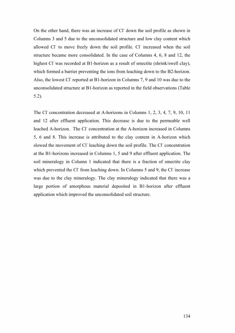
134

On the other hand, there was an increase of Cl- down the soil profile as shown in

Columns 3 and 5 due to the unconsolidated structure and low clay content which

allowed Cl- to move freely down the soil profile. Cl- increased when the soil

structure became more consolidated. In the case of Columns 4, 6, 8 and 12, the

highest Cl- was recorded at B1-horizon as a result of smectite (shrink/swell clay),

which formed a barrier preventing the ions from leaching down to the B2-horizon.

Also, the lowest Cl- reported at B1-horizon in Columns 7, 9 and 10 was due to the

unconsolidated structure at B1-horizon as reported in the field observations (Table

5.2).

The Cl- concentration decreased at A-horizons in Columns 1, 2, 3, 4, 7, 9, 10, 11

and 12 after effluent application. This decrease is due to the permeable well

leached A-horizon. The Cl- concentration at the A-horizon increased in Columns

5, 6 and 8. This increase is attributed to the clay content in A-horizon which

slowed the movement of Cl- leaching down the soil profile. The Cl- concentration

at the B1-horizons increased in Columns 1, 5 and 9 after effluent application. The

soil mineralogy in Column 1 indicated that there is a fraction of smectite clay

which prevented the Cl- from leaching down. In Columns 5 and 9, the Cl- increase

was due to the clay mineralogy. The clay mineralogy indicated that there was a

large portion of amorphous material deposited in B1-horizon after effluent

application which improved the unconsolidated soil structure.

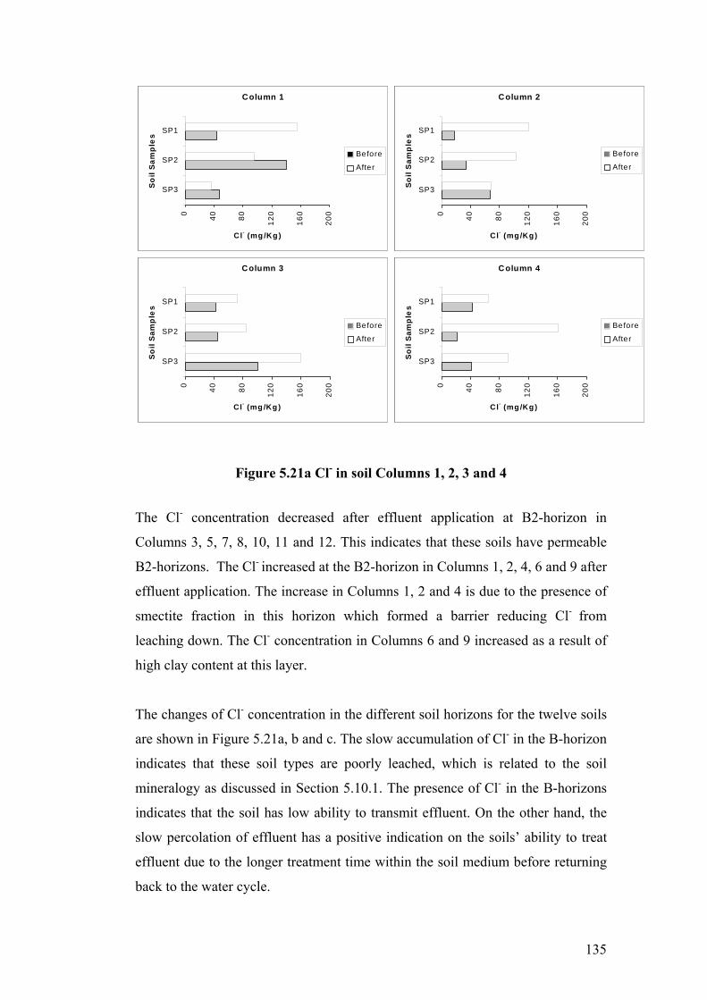
135

Figure 5.21a Cl- in soil Columns 1, 2, 3 and 4

The Cl- concentration decreased after effluent application at B2-horizon in

Columns 3, 5, 7, 8, 10, 11 and 12. This indicates that these soils have permeable

B2-horizons. The Cl- increased at the B2-horizon in Columns 1, 2, 4, 6 and 9 after

effluent application. The increase in Columns 1, 2 and 4 is due to the presence of

smectite fraction in this horizon which formed a barrier reducing Cl- from

leaching down. The Cl- concentration in Columns 6 and 9 increased as a result of

high clay content at this layer.

The changes of Cl- concentration in the different soil horizons for the twelve soils

are shown in Figure 5.21a, b and c. The slow accumulation of Cl- in the B-horizon

indicates that these soil types are poorly leached, which is related to the soil

mineralogy as discussed in Section 5.10.1. The presence of Cl- in the B-horizons

indicates that the soil has low ability to transmit effluent. On the other hand, the

slow percolation of effluent has a positive indication on the soils’ ability to treat

effluent due to the longer treatment time within the soil medium before returning

back to the water cycle.

Column 1

0 40 80 120

160

200

SP3

SP2

SP1

So

il S

amp

les

C l- (mg /Kg)

Before

After

Column 2

0 40 80 120

160

200

SP3

SP2

SP1

So

il S

amp

les

C l- (mg /Kg)

Before

After

C olumn 3

0 40 80 120

160

200

SP3

SP2

SP1

So

il S

amp

les

C l- (mg /Kg)

Before

After

C olumn 4

0 40 80 120

160

200

SP3

SP2

SP1

So

il S

amp

les

C l- (mg /Kg)

Before

After

Column 1

0 40 80 120

160

200

SP3

SP2

SP1

So

il S

amp

les

C l- (mg /Kg)

Before

After

Column 2

0 40 80 120

160

200

SP3

SP2

SP1

So

il S

amp

les

C l- (mg /Kg)

Before

After

C olumn 3

0 40 80 120

160

200

SP3

SP2

SP1

So

il S

amp

les

C l- (mg /Kg)

Before

After

C olumn 4

0 40 80 120

160

200

SP3

SP2

SP1

So

il S

amp

les

C l- (mg /Kg)

Before

After

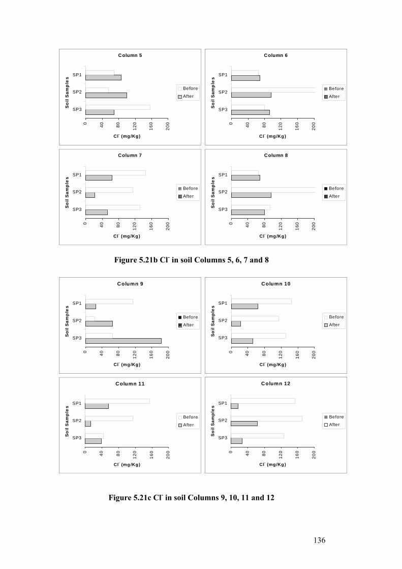
136

Figure 5.21b Cl- in soil Columns 5, 6, 7 and 8

Figure 5.21c Cl- in soil Columns 9, 10, 11 and 12

Column 5

0 40 80 120

160

200

SP3

SP2

SP1

So

il S

amp

les

Cl- (mg/Kg)

Before

After

Column 6

0 40 80 120

160

200

SP3

SP2

SP1

So

il S

amp

les

Cl- (mg/Kg)

Before

After

Column 7

0 40 80 120

160

200

SP3

SP2

SP1

So

il S

amp

les

Cl- (mg/Kg)

Before

After

Column 8

0 40 80 120

160

200

SP3

SP2

SP1

So

il S

amp

les

Cl- (mg/Kg)

Before

After

Column 5

0 40 80 120

160

200

SP3

SP2

SP1

So

il S

amp

les

Cl- (mg/Kg)

Before

After

Column 6

0 40 80 120

160

200

SP3

SP2

SP1

So

il S

amp

les

Cl- (mg/Kg)

Before

After

Column 7

0 40 80 120

160

200

SP3

SP2

SP1

So

il S

amp

les

Cl- (mg/Kg)

Before

After

Column 8

0 40 80 120

160

200

SP3

SP2

SP1

So

il S

amp

les

Cl- (mg/Kg)

Before

After

Column 9

0 40 80 120

160

200

SP3

SP2

SP1

So

il S

amp

les

Cl- (mg/Kg)

Before

After

Column 10

0 40 80 120

160

200

SP3

SP2

SP1

So

il S

amp

les

Cl- (mg/Kg)

Before

After

Column 11

0 40 80 120

160

200

SP3

SP2

SP1

So

il S

amp

les

Cl- (mg/Kg)

Before

After

Column 12

0 40 80 120

160

200

SP3

SP2

SP1

So

il S

amp

les

Cl- (mg/Kg)

Before

After

Column 9

0 40 80 120

160

200

SP3

SP2

SP1

So

il S

amp

les

Cl- (mg/Kg)

Before

After

Column 10

0 40 80 120

160

200

SP3

SP2

SP1

So

il S

amp

les

Cl- (mg/Kg)

Before

After

Column 11

0 40 80 120

160

200

SP3

SP2

SP1

So

il S

amp

les

Cl- (mg/Kg)

Before

After

Column 12

0 40 80 120

160

200

SP3

SP2

SP1

So

il S

amp

les

Cl- (mg/Kg)

Before

After

137

5.10.7 Nutrients (P and N)

In general, phosphorus (P) exists in the soil in various forms, in solid form as a

part of the mineral fractions or soluble form such as orthophosphate. P as well as

nitrogen (N) are important nutrients for plant growth. Also, P quantities in the soil

vary with the soil type, OM, rainfall, hydrology and vegetation in the area (Brady

and Weil, 2002). The OM in the soil would have a large impact on the nutrient

availability based on the OM stability. In the case where OM levels are stabilised,

the nutrient release and uptake processes are managed by this existing OM in the

soil. However, if the OM is destabilised (decrease/increase OM due to the soil

composition), the release and uptake of the nutrients is controlled by the new

amount of OM available. The release and uptake of P by the OM can reduce or

increase the soil capacity to hold nutrients from the discharged effluent.

The highest P value at A-horizon in the original soil samples was reported in

Columns 1, 2, 3, 5, 8 and 11. This is a result of the high OM (over 5%), which

facilitates the P uptake mechanism. In general, the accumulation of P at A-

horizons is due to the OM, and the P levels decreased down the soil profile with

the decrease of OM in these columns as presented in Figures 5.22a, b and c. The

P content increased down the soil profile in Columns 6, 10 and 12 due to the high

OM in these soils. The P concentration was the highest at B1-horizon in Columns

1, 6, 8 and 10 due to the unconsolidated structure between A and B2-horizons

which allowed higher OM to be accumulated in the B1-horizon. Overall the

highest value was reported in Column 10. This is due to stabilised organic matter

content and clay content through the soil profile.

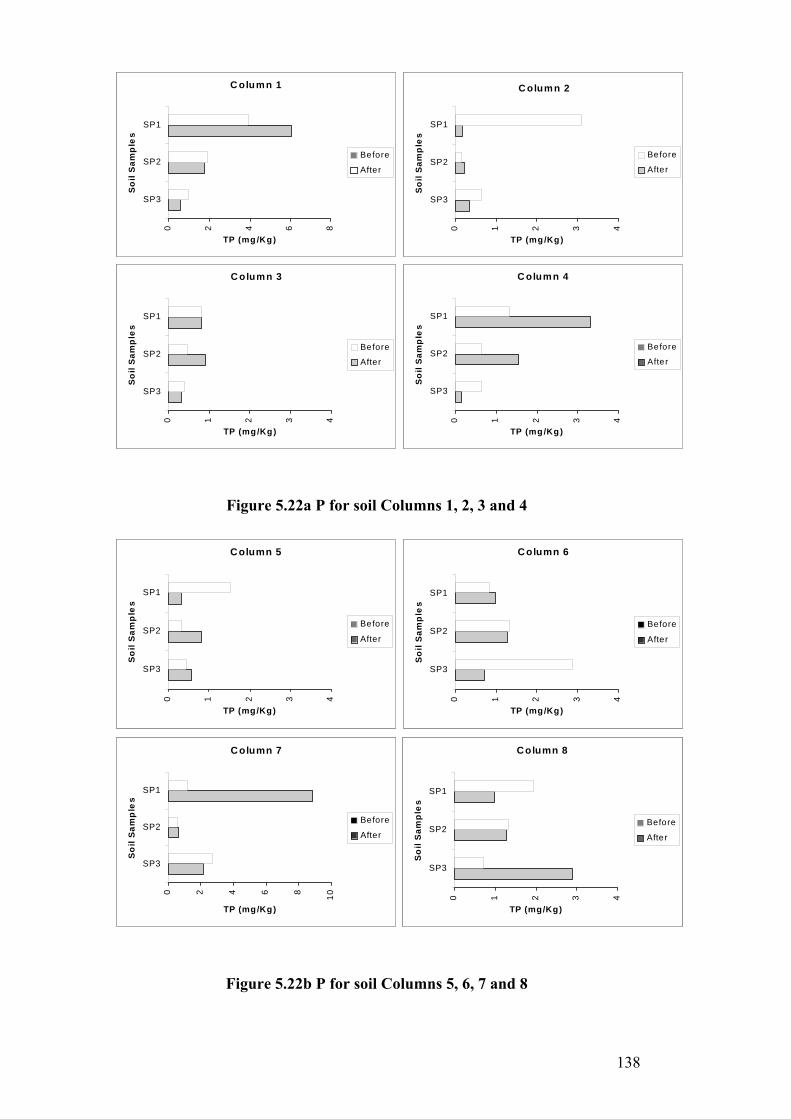
138

Figure 5.22a P for soil Columns 1, 2, 3 and 4

Figure 5.22b P for soil Columns 5, 6, 7 and 8

C olumn 1

0 2 4 6 8

SP3

SP2

SP1S

oil

Sam

ple

s

TP (mg /Kg)

Before

After

C olumn 2

0 1 2 3 4

SP3

SP2

SP1

So

il S

amp

les

TP (mg /Kg)

Before

After

C olumn 3

0 1 2 3 4

SP3

SP2

SP1

So

il S

amp

les

TP (mg /Kg)

Before

After

C olumn 4

0 1 2 3 4

SP3

SP2

SP1

So

il S

amp

les

TP (mg /Kg)

Before

After

C olumn 1

0 2 4 6 8

SP3

SP2

SP1S

oil

Sam

ple

s

TP (mg /Kg)

Before

After

C olumn 2

0 1 2 3 4

SP3

SP2

SP1

So

il S

amp

les

TP (mg /Kg)

Before

After

C olumn 3

0 1 2 3 4

SP3

SP2

SP1

So

il S

amp

les

TP (mg /Kg)

Before

After

C olumn 4

0 1 2 3 4

SP3

SP2

SP1

So

il S

amp

les

TP (mg /Kg)

Before

After

Column 5

0 1 2 3 4

SP3

SP2

SP1

So

il S

amp

les

TP (mg/Kg)

Before

After

Column 6

0 1 2 3 4

SP3

SP2

SP1

So

il S

amp

les

TP (mg/Kg)

Before

After

Column 7

0 2 4 6 8 10

SP3

SP2

SP1

So

il S

amp

les

TP (mg/Kg)

Before

After

Column 8

0 1 2 3 4

SP3

SP2

SP1

So

il S

amp

les

TP (mg/Kg)

Before

After

Column 5

0 1 2 3 4

SP3

SP2

SP1

So

il S

amp

les

TP (mg/Kg)

Before

After

C olumn 6

0 1 2 3 4

SP3

SP2

SP1

So

il S

amp

les

TP (mg/Kg)

Before

After

C olumn 7

0 2 4 6 8 10

SP3

SP2

SP1

So

il S

amp

les

TP (mg/Kg)

Before

After

Column 8

0 1 2 3 4

SP3

SP2

SP1

So

il S

amp

les

TP (mg/Kg)

Before

After

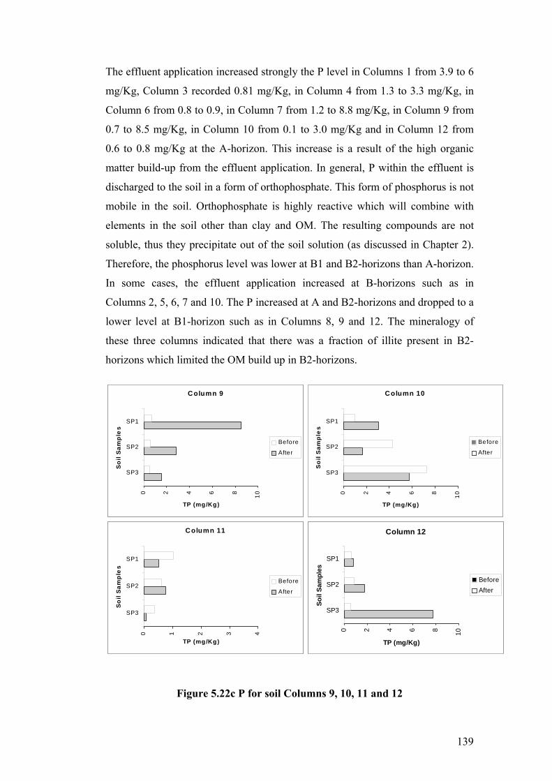
139

The effluent application increased strongly the P level in Columns 1 from 3.9 to 6

mg/Kg, Column 3 recorded 0.81 mg/Kg, in Column 4 from 1.3 to 3.3 mg/Kg, in

Column 6 from 0.8 to 0.9, in Column 7 from 1.2 to 8.8 mg/Kg, in Column 9 from

0.7 to 8.5 mg/Kg, in Column 10 from 0.1 to 3.0 mg/Kg and in Column 12 from

0.6 to 0.8 mg/Kg at the A-horizon. This increase is a result of the high organic

matter build-up from the effluent application. In general, P within the effluent is

discharged to the soil in a form of orthophosphate. This form of phosphorus is not

mobile in the soil. Orthophosphate is highly reactive which will combine with

elements in the soil other than clay and OM. The resulting compounds are not

soluble, thus they precipitate out of the soil solution (as discussed in Chapter 2).

Therefore, the phosphorus level was lower at B1 and B2-horizons than A-horizon.

In some cases, the effluent application increased at B-horizons such as in

Columns 2, 5, 6, 7 and 10. The P increased at A and B2-horizons and dropped to a

lower level at B1-horizon such as in Columns 8, 9 and 12. The mineralogy of

these three columns indicated that there was a fraction of illite present in B2-

horizons which limited the OM build up in B2-horizons.

Figure 5.22c P for soil Columns 9, 10, 11 and 12

Column 9

0 2 4 6 8 10

SP3

SP2

SP1

So

il S

amp

les

TP (mg/Kg)

Before

After

Column 10

0 2 4 6 8 10

SP3

SP2

SP1

So

il S

amp

les

TP (mg/Kg)

Before

After

Column 11

0 1 2 3 4

SP3

SP2

SP1

So

il S

amp

les

TP (mg/Kg)

Before

After

Column 12

0 2 4 6 8 10

SP3

SP2

SP1

Soil

Sam

ples

TP (mg/Kg)

BeforeAfter

Column 9

0 2 4 6 8 10

SP3

SP2

SP1

So

il S

amp

les

TP (mg/Kg)

Before

After

Column 10

0 2 4 6 8 10

SP3

SP2

SP1

So

il S

amp

les

TP (mg/Kg)

Before

After

Column 11

0 1 2 3 4

SP3

SP2

SP1

So

il S

amp

les

TP (mg/Kg)

Before

After

Column 12

0 2 4 6 8 10

SP3

SP2

SP1

Soil

Sam

ples

TP (mg/Kg)

BeforeAfter

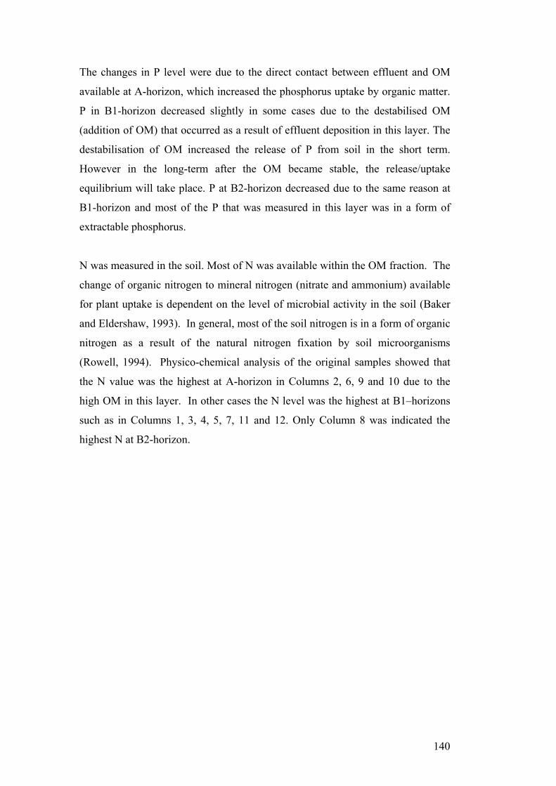
140

The changes in P level were due to the direct contact between effluent and OM

available at A-horizon, which increased the phosphorus uptake by organic matter.

P in B1-horizon decreased slightly in some cases due to the destabilised OM

(addition of OM) that occurred as a result of effluent deposition in this layer. The

destabilisation of OM increased the release of P from soil in the short term.

However in the long-term after the OM became stable, the release/uptake

equilibrium will take place. P at B2-horizon decreased due to the same reason at

B1-horizon and most of the P that was measured in this layer was in a form of

extractable phosphorus.

N was measured in the soil. Most of N was available within the OM fraction. The

change of organic nitrogen to mineral nitrogen (nitrate and ammonium) available

for plant uptake is dependent on the level of microbial activity in the soil (Baker

and Eldershaw, 1993). In general, most of the soil nitrogen is in a form of organic

nitrogen as a result of the natural nitrogen fixation by soil microorganisms

(Rowell, 1994). Physico-chemical analysis of the original samples showed that

the N value was the highest at A-horizon in Columns 2, 6, 9 and 10 due to the

high OM in this layer. In other cases the N level was the highest at B1–horizons

such as in Columns 1, 3, 4, 5, 7, 11 and 12. Only Column 8 was indicated the

highest N at B2-horizon.

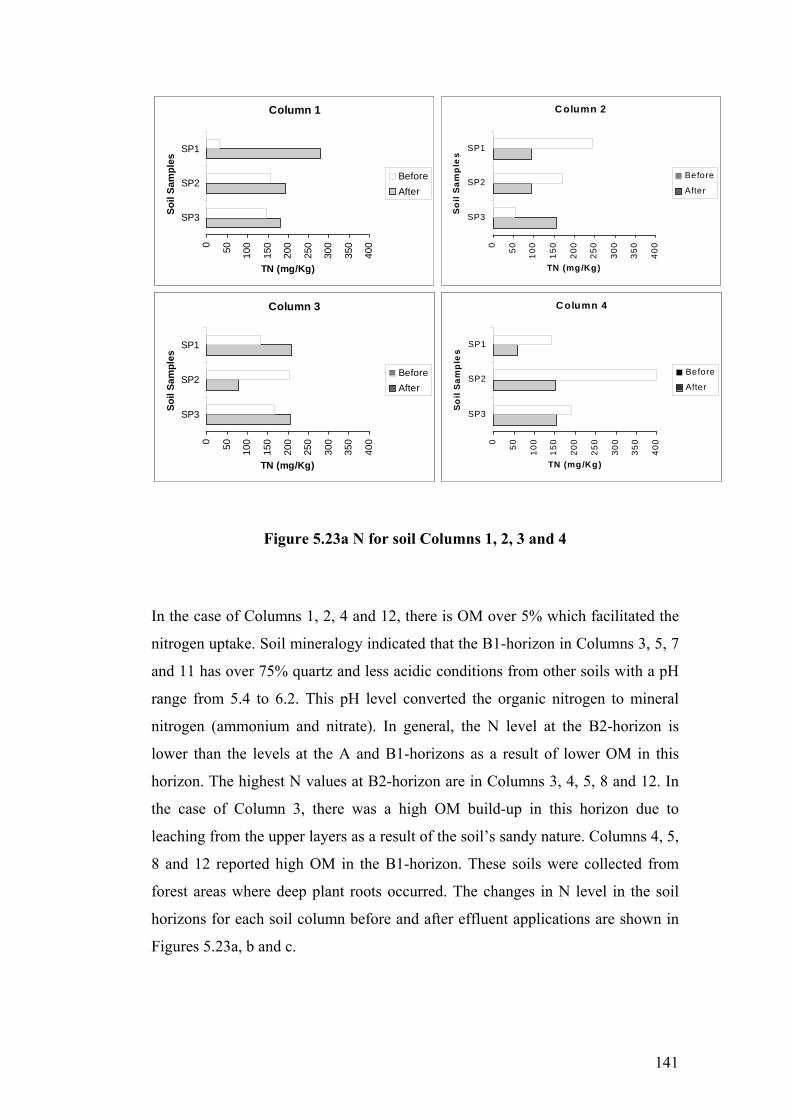
141

Figure 5.23a N for soil Columns 1, 2, 3 and 4

In the case of Columns 1, 2, 4 and 12, there is OM over 5% which facilitated the

nitrogen uptake. Soil mineralogy indicated that the B1-horizon in Columns 3, 5, 7

and 11 has over 75% quartz and less acidic conditions from other soils with a pH

range from 5.4 to 6.2. This pH level converted the organic nitrogen to mineral

nitrogen (ammonium and nitrate). In general, the N level at the B2-horizon is

lower than the levels at the A and B1-horizons as a result of lower OM in this

horizon. The highest N values at B2-horizon are in Columns 3, 4, 5, 8 and 12. In

the case of Column 3, there was a high OM build-up in this horizon due to

leaching from the upper layers as a result of the soil’s sandy nature. Columns 4, 5,

8 and 12 reported high OM in the B1-horizon. These soils were collected from

forest areas where deep plant roots occurred. The changes in N level in the soil

horizons for each soil column before and after effluent applications are shown in

Figures 5.23a, b and c.

Column 1

0 50 100

150

200

250

300

350

400

SP3

SP2

SP1

Soil

Sam

ples

TN (mg/Kg)

BeforeAfter

Column 2

0 50 100

150

200

250

300

350

400

SP3

SP2

SP1

So

il S

amp

les

TN (mg/Kg)

Before

After

Column 3

0 50 100

150

200

250

300

350

400

SP3

SP2

SP1

Soil

Sam

ples

TN (mg/Kg)

BeforeAfter

C olumn 4

0 50 100

150

200

250

300

350

400

SP3

SP2

SP1

So

il S

amp

les

TN (mg/Kg)

Before

After

Column 1

0 50 100

150

200

250

300

350

400

SP3

SP2

SP1

Soil

Sam

ples

TN (mg/Kg)

BeforeAfter

Column 2

0 50 100

150

200

250

300

350

400

SP3

SP2

SP1

So

il S

amp

les

TN (mg/Kg)

Before

After

Column 3

0 50 100

150

200

250

300

350

400

SP3

SP2

SP1

Soil

Sam

ples

TN (mg/Kg)

BeforeAfter

C olumn 4

0 50 100

150

200

250

300

350

400

SP3

SP2

SP1

So

il S

amp

les

TN (mg/Kg)

Before

After

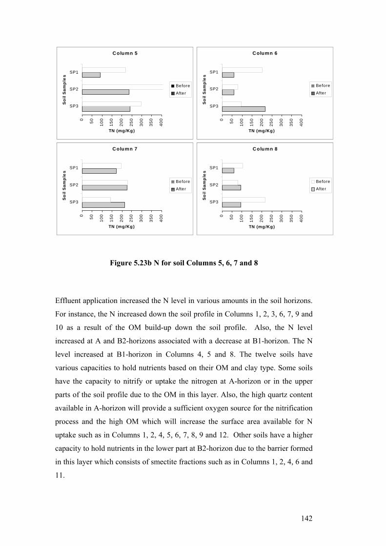
142

Figure 5.23b N for soil Columns 5, 6, 7 and 8

Effluent application increased the N level in various amounts in the soil horizons.

For instance, the N increased down the soil profile in Columns 1, 2, 3, 6, 7, 9 and

10 as a result of the OM build-up down the soil profile. Also, the N level

increased at A and B2-horizons associated with a decrease at B1-horizon. The N

level increased at B1-horizon in Columns 4, 5 and 8. The twelve soils have

various capacities to hold nutrients based on their OM and clay type. Some soils

have the capacity to nitrify or uptake the nitrogen at A-horizon or in the upper

parts of the soil profile due to the OM in this layer. Also, the high quartz content

available in A-horizon will provide a sufficient oxygen source for the nitrification

process and the high OM which will increase the surface area available for N

uptake such as in Columns 1, 2, 4, 5, 6, 7, 8, 9 and 12. Other soils have a higher

capacity to hold nutrients in the lower part at B2-horizon due to the barrier formed

in this layer which consists of smectite fractions such as in Columns 1, 2, 4, 6 and

11.

C olumn 5

0 50 100

150

200

250

300

350

400

SP3

SP2

SP1

So

il S

amp

les

TN (mg/Kg)

Before

After

Column 6

0 50 100

150

200

250

300

350

400

SP3

SP2

SP1

So

il S

amp

les

TN (mg/Kg)

Before

After

Column 7

0 50 100

150

200

250

300

350

400

SP3

SP2

SP1

So

il S

amp

les

TN (mg/Kg)

Before

After

Column 8

0 50 100

150

200

250

300

350

400

SP3

SP2

SP1

So

il S

amp

les

TN (mg/Kg)

Before

After

C olumn 5

0 50 100

150

200

250

300

350

400

SP3

SP2

SP1

So

il S

amp

les

TN (mg/Kg)

Before

After

Column 6

0 50 100

150

200

250

300

350

400

SP3

SP2

SP1

So

il S

amp

les

TN (mg/Kg)

Before

After

Column 7

0 50 100

150

200

250

300

350

400

SP3

SP2

SP1

So

il S

amp

les

TN (mg/Kg)

Before

After

Column 8

0 50 100

150

200

250

300

350

400

SP3

SP2

SP1

So

il S

amp

les

TN (mg/Kg)

Before

After

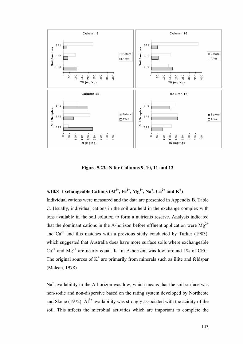
143

Figure 5.23c N for Columns 9, 10, 11 and 12

5.10.8 Exchangeable Cations (Al3+, Fe2+, Mg2+, Na+, Ca2+ and K+)

Individual cations were measured and the data are presented in Appendix B, Table

C. Usually, individual cations in the soil are held in the exchange complex with

ions available in the soil solution to form a nutrients reserve. Analysis indicated

that the dominant cations in the A-horizon before effluent application were Mg2+

and Ca2+ and this matches with a previous study conducted by Turker (1983),

which suggested that Australia does have more surface soils where exchangeable

Ca2+ and Mg2+ are nearly equal. K+ in A-horizon was low, around 1% of CEC.

The original sources of K+ are primarily from minerals such as illite and feldspar

(Mclean, 1978).

Na+ availability in the A-horizon was low, which means that the soil surface was

non-sodic and non-dispersive based on the rating system developed by Northcote

and Skene (1972). Al3+ availability was strongly associated with the acidity of the

soil. This affects the microbial activities which are important to complete the

Column 9

0 50 100

150

200

250

300

350

400

SP3

SP2

SP1

So

il S

amp

les

TN (mg/Kg)

Before

After

Column 10

0 50 100

150

200

250

300

350

400

SP3

SP2

SP1

So

il S

amp

les

TN (mg/Kg)

Before

After

Column 11

0 50 100

150

200

250

300

350

400

SP3

SP2

SP1

So

il S

amp

les

TN (mg/Kg)

Before

After

C olumn 12

0 50 100

150

200

250

300

350

400

SP3

SP2

SP1

So

il S

amp

les

TN (mg/Kg)

Before

After

Column 9

0 50 100

150

200

250

300

350

400

SP3

SP2

SP1

So

il S

amp

les

TN (mg/Kg)

Before

After

Column 10

0 50 100

150

200

250

300

350

400

SP3

SP2

SP1

So

il S

amp

les

TN (mg/Kg)

Before

After

Column 11

0 50 100

150

200

250

300

350

400

SP3

SP2

SP1

So

il S

amp

les

TN (mg/Kg)

Before

After

C olumn 12

0 50 100

150

200

250

300

350

400

SP3

SP2

SP1

So

il S

amp

les

TN (mg/Kg)

Before

After

144

effluent renovation processes. Also, low concentrations of Al3+ were reported in

the A-horizons before effluent application which meant that there was reduced

toxic medium for effluent renovation.

The individual exchangeable cations measured in the B-horizons before effluent

application showed various Ca2+ concentration values. The concentration

decreased down the soil column. This drop is attributed to the high Mg2+

concentration. An excess of one cation may inhibit the uptake of another (Baker

and Eldershaw, 1993). The Mg2+ concentration increased in the B1-horizon, and

B2-horizon as a result of cations leaching down the soil profile carried by effluent.

In the case of Na+, the concentration increased in the B1-horizon and B2-horizon

in most soils. This is a common result of increasing the soluble salts within the

soil profile. The K+ was less in the B1-horizon and in the B2-horizon. There was a

slight presence of Al3+ in the A-horizon which increased down the soil profile

when the pH dropped below 5 in the original soil samples. Effluent application

improved the soil acidity (less acidic) which decreased the Al3+ content in the soil

profile.

The exchangeable cation analysis is plotted in Figures 5.24, 5.25 and 5.26.

Effluent application affected the soil solution adversely in some cases and

sometimes advantageously. It reduced the acidity of the soil at the different soil

horizons. The drop in Mg2+ associated with improved Ca2+ availability was a

positive indication towards balancing the ratio between Mg2+ to Ca2+. Effluent

application increased the Na+ level in the A-horizon and decreased in some cases

in the B1-horizon and increased in the B2-horizon. The continuous effluent

application with increase of Na+ could lead to soil on the surface to disperse

which will form or precipitate a white or pale colored compound on the soil

surface due to the high salts content. In general, if the soil is physically crusted or

dispersed, it indicates the amount of OM in the soil has decreased and/or erosion

has occurred. Also, the soil will have a low aggregate stability under wet

conditions which will reduces the infiltrative rate (USDA, 2001).

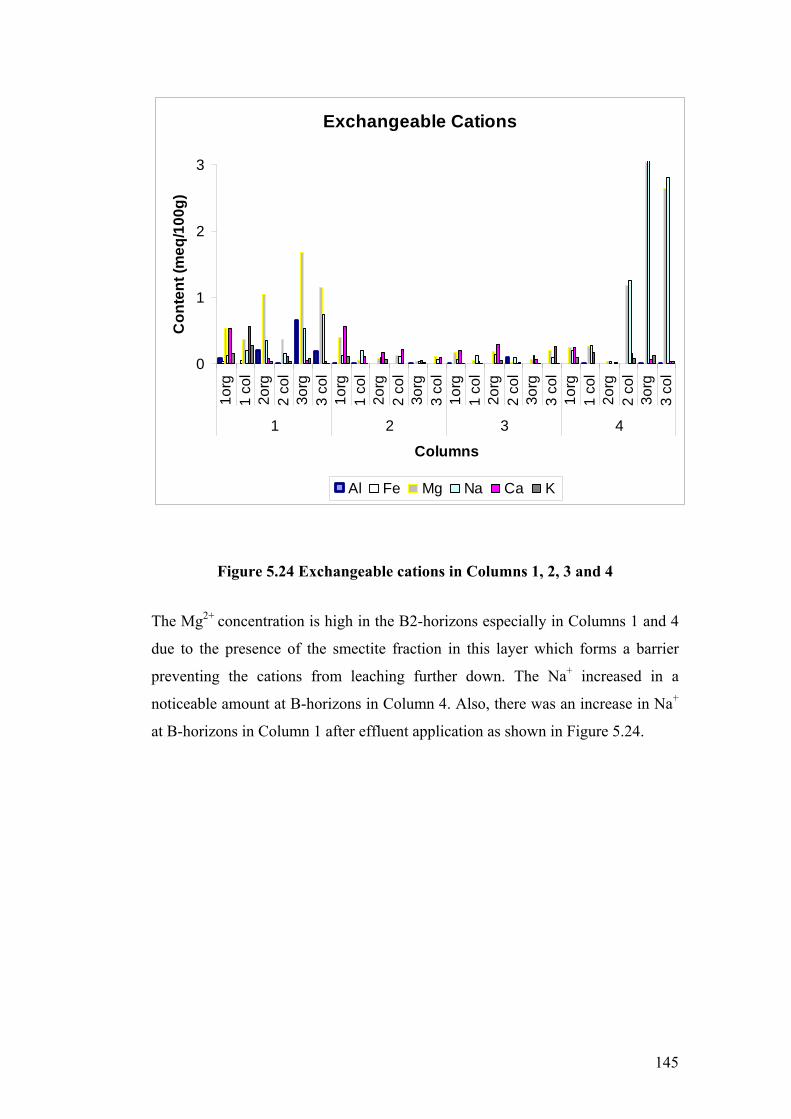
145

Exchangeable Cations

0

1

2

3

1org

1 co

l2o

rg2

col

3org

3 co

l1o

rg1

col

2org

2 co

l3o

rg3

col

1org

1 co

l2o

rg2

col

3org

3 co

l1o

rg1

col

2org

2 co

l3o

rg3

col

1 2 3 4

Columns

Con

tent

(meq

/100

g)

Al Fe Mg Na Ca K

Figure 5.24 Exchangeable cations in Columns 1, 2, 3 and 4

The Mg2+ concentration is high in the B2-horizons especially in Columns 1 and 4

due to the presence of the smectite fraction in this layer which forms a barrier

preventing the cations from leaching further down. The Na+ increased in a

noticeable amount at B-horizons in Column 4. Also, there was an increase in Na+

at B-horizons in Column 1 after effluent application as shown in Figure 5.24.

146


0.00

1.00

2.00

3.00

1org

1 co

l2o

rg2

col

3org

3 co

l1o

rg1

col

2org

2 co

l3o

rg3

col

1org

1 co

l2o

rg2

col

3org

3 co

l1o

rg1

col

2org

2 co

l3o

rg3

col

5 6 7 8

Columns

Con

tent

(meq

/100

g)

Al Fe Mg Na Ca K


The exchangeable cations distribution for Columns 5, 6, 7 and 8 is shown in

Figure 5.25. The Mg2+ was dominant in these four columns and especially

Column 8 due to the unconsolidated structure at B1-horizons. Also, the Na+

content was high in Column 6 especially at B2-horizon and in Column 8

especially in the original sample before effluent application at B1-horizon. The

lowest cations level was in Column 7 and the highest cations content in Column 8.

Figure 5.26 shows the exchangeable cations distribution for Columns 9, 10, 11

and 12. Also, the Mg2+ was dominant in these four columns especially Column

12. The Na+ content was high in Column 11 especially at B2-horizon. In general,

the other three columns have low exchangeable cations except in the B2-horizon

in Column 11.

147


0.00

1.00

2.00

3.00

1org

1 co

l2o

rg2

col

3org

3 co

l1o

rg1

col

2org

2 co

l3o

rg3

col

1org

1 co

l2o

rg2

col

3org

3 co

l1o

rg1c

ol2o

rg2

col

3org

9 10 11 12

Columns

Con

tent

(meq

/100

g)

Al Fe Mg Na Ca K


5.10.9 Ca:Mg Ratio and Exchangeable Sodium Percentage (ESP)

Determination of the soil fertility Ca:Mg ratio is based on various nutrients such

as N, P, Ca2+ and Mg2+ which are essential for plant growth. The Ca:Mg ratio is

used to evaluate the cation balance in the soil solution , especially if the dominant

cation in the subsurface layer was Mg2+, which was the case in most columns.

Availability of essential nutrients is influenced by soil pH. Ca2+ deficiencies occur

when the soil pH is less than 5.0. Also, Mg2+ concentration is determined largely

by soil pH quality.

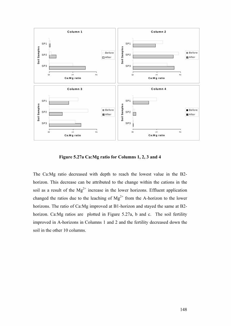
148

Figure 5.27a Ca:Mg ratio for Columns 1, 2, 3 and 4 The Ca:Mg ratio decreased with depth to reach the lowest value in the B2-

horizon. This decrease can be attributed to the change within the cations in the

soil as a result of the Mg2+ increase in the lower horizons. Effluent application

changed the ratios due to the leaching of Mg2+ from the A-horizon to the lower

horizons. The ratio of Ca:Mg improved at B1-horizon and stayed the same at B2-

horizon. Ca:Mg ratios are plotted in Figure 5.27a, b and c. The soil fertility

improved in A-horizons in Columns 1 and 2 and the fertility decreased down the

soil in the other 10 columns.

C olumn 1

0 1 2

SP3

SP2

SP1

So

il S

amp

les

Ca:M g ratio

Before

After

C olumn 2

0 1 2

SP3

SP2

SP1

So

il S

amp

les

Ca:M g ratio

Before

After

C olumn 3

0 1 2

SP3

SP2

SP1

So

il S

amp

les

Ca:M g ratio

Before

After

C olumn 4

0 1 2

SP3

SP2

SP1

So

il S

amp

les

Ca:M g ratio

Before

After

C olumn 1

0 1 2

SP3

SP2

SP1

So

il S

amp

les

Ca:M g ratio

Before

After

C olumn 2

0 1 2

SP3

SP2

SP1

So

il S

amp

les

Ca:M g ratio

Before

After

C olumn 3

0 1 2

SP3

SP2

SP1

So

il S

amp

les

Ca:M g ratio

Before

After

C olumn 4

0 1 2

SP3

SP2

SP1

So

il S

amp

les

Ca:M g ratio

Before

After

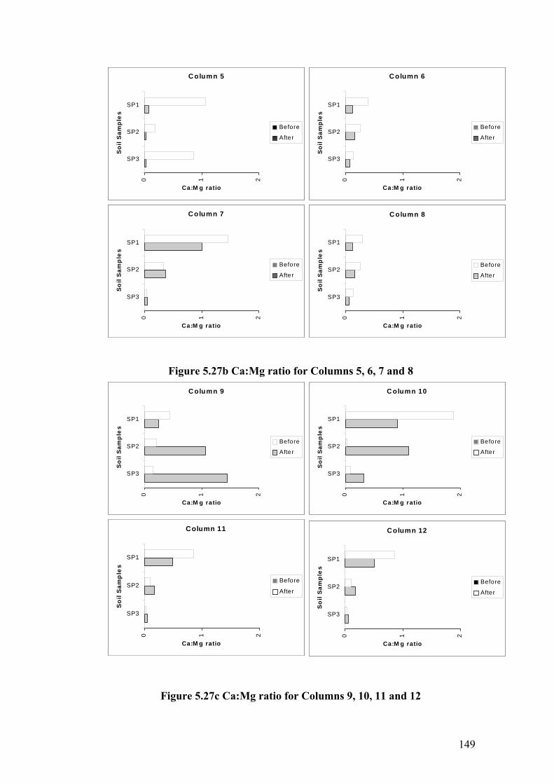
149

Figure 5.27b Ca:Mg ratio for Columns 5, 6, 7 and 8

Figure 5.27c Ca:Mg ratio for Columns 9, 10, 11 and 12

C olumn 5

0 1 2

SP3

SP2

SP1

So

il S

amp

les

Ca:M g ratio

Before

After

Column 6

0 1 2

SP3

SP2

SP1

So

il S

amp

les

Ca:M g ratio

Before

After

Column 7

0 1 2

SP3

SP2

SP1

So

il S

amp

les

Ca:M g ratio

Before

After

C olumn 8

0 1 2

SP3

SP2

SP1

So

il S

amp

les

Ca:M g ratio

Before

After

C olumn 5

0 1 2

SP3

SP2

SP1

So

il S

amp

les

Ca:M g ratio

Before

After

Column 6

0 1 2

SP3

SP2

SP1

So

il S

amp

les

Ca:M g ratio

Before

After

Column 7

0 1 2

SP3

SP2

SP1

So

il S

amp

les

Ca:M g ratio

Before

After

C olumn 8

0 1 2

SP3

SP2

SP1

So

il S

amp

les

Ca:M g ratio

Before

After

C olumn 9

0 1 2

SP3

SP2

SP1

So

il S

amp

les

Ca:M g ratio

Before

After

C olumn 10

0 1 2

SP3

SP2

SP1

So

il S

amp

les

Ca:M g ratio

Before

After

Column 11

0 1 2

SP3

SP2

SP1

So

il S

amp

les

Ca:M g ratio

Before

After

Column 12

0 1 2

SP3

SP2

SP1

So

il S

amp

les

Ca:M g ratio

Before

After

C olumn 9

0 1 2

SP3

SP2

SP1

So

il S

amp

les

Ca:M g ratio

Before

After

C olumn 10

0 1 2

SP3

SP2

SP1

So

il S

amp

les

Ca:M g ratio

Before

After

Column 11

0 1 2

SP3

SP2

SP1

So

il S

amp

les

Ca:M g ratio

Before

After

Column 12

0 1 2

SP3

SP2

SP1

So

il S

amp

les

Ca:M g ratio

Before

After

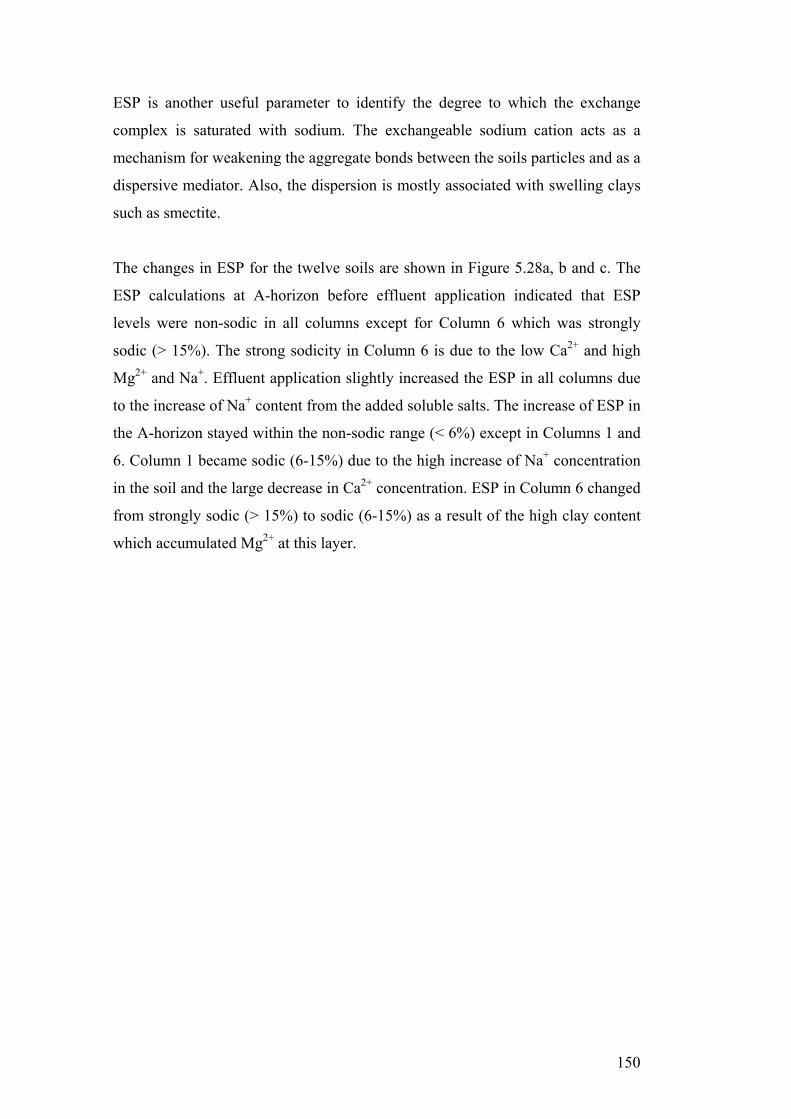
150

ESP is another useful parameter to identify the degree to which the exchange

complex is saturated with sodium. The exchangeable sodium cation acts as a

mechanism for weakening the aggregate bonds between the soils particles and as a

dispersive mediator. Also, the dispersion is mostly associated with swelling clays

such as smectite.

The changes in ESP for the twelve soils are shown in Figure 5.28a, b and c. The

ESP calculations at A-horizon before effluent application indicated that ESP

levels were non-sodic in all columns except for Column 6 which was strongly

sodic (> 15%). The strong sodicity in Column 6 is due to the low Ca2+ and high

Mg2+ and Na+. Effluent application slightly increased the ESP in all columns due

to the increase of Na+ content from the added soluble salts. The increase of ESP in

the A-horizon stayed within the non-sodic range (< 6%) except in Columns 1 and

6. Column 1 became sodic (6-15%) due to the high increase of Na+ concentration

in the soil and the large decrease in Ca2+ concentration. ESP in Column 6 changed

from strongly sodic (> 15%) to sodic (6-15%) as a result of the high clay content

which accumulated Mg2+ at this layer.

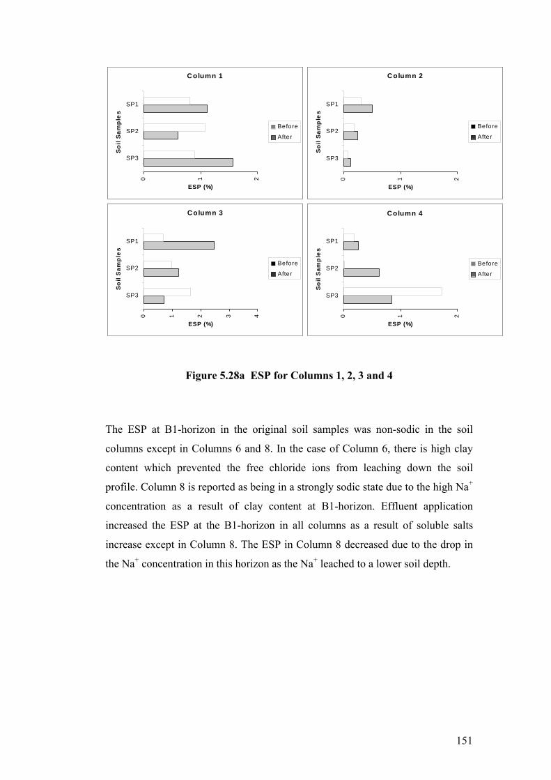
151

Figure 5.28a ESP for Columns 1, 2, 3 and 4

The ESP at B1-horizon in the original soil samples was non-sodic in the soil

columns except in Columns 6 and 8. In the case of Column 6, there is high clay

content which prevented the free chloride ions from leaching down the soil

profile. Column 8 is reported as being in a strongly sodic state due to the high Na+

concentration as a result of clay content at B1-horizon. Effluent application

increased the ESP at the B1-horizon in all columns as a result of soluble salts

increase except in Column 8. The ESP in Column 8 decreased due to the drop in

the Na+ concentration in this horizon as the Na+ leached to a lower soil depth.

C olumn 1

0 1 2

SP3

SP2

SP1

So

il S

amp

les

ESP (%)

Before

After

C olumn 2

0 1 2

SP3

SP2

SP1

So

il S

amp

les

ESP (%)

Before

After

C olumn 3

0 1 2 3 4

SP3

SP2

SP1

So

il S

amp

les

ESP (%)

Before

After

C olumn 4

0 1 2

SP3

SP2

SP1

So

il S

amp

les

ESP (%)

Before

After

C olumn 1

0 1 2

SP3

SP2

SP1

So

il S

amp

les

ESP (%)

Before

After

C olumn 2

0 1 2

SP3

SP2

SP1

So

il S

amp

les

ESP (%)

Before

After

C olumn 3

0 1 2 3 4

SP3

SP2

SP1

So

il S

amp

les

ESP (%)

Before

After

C olumn 4

0 1 2

SP3

SP2

SP1

So

il S

amp

les

ESP (%)

Before

After

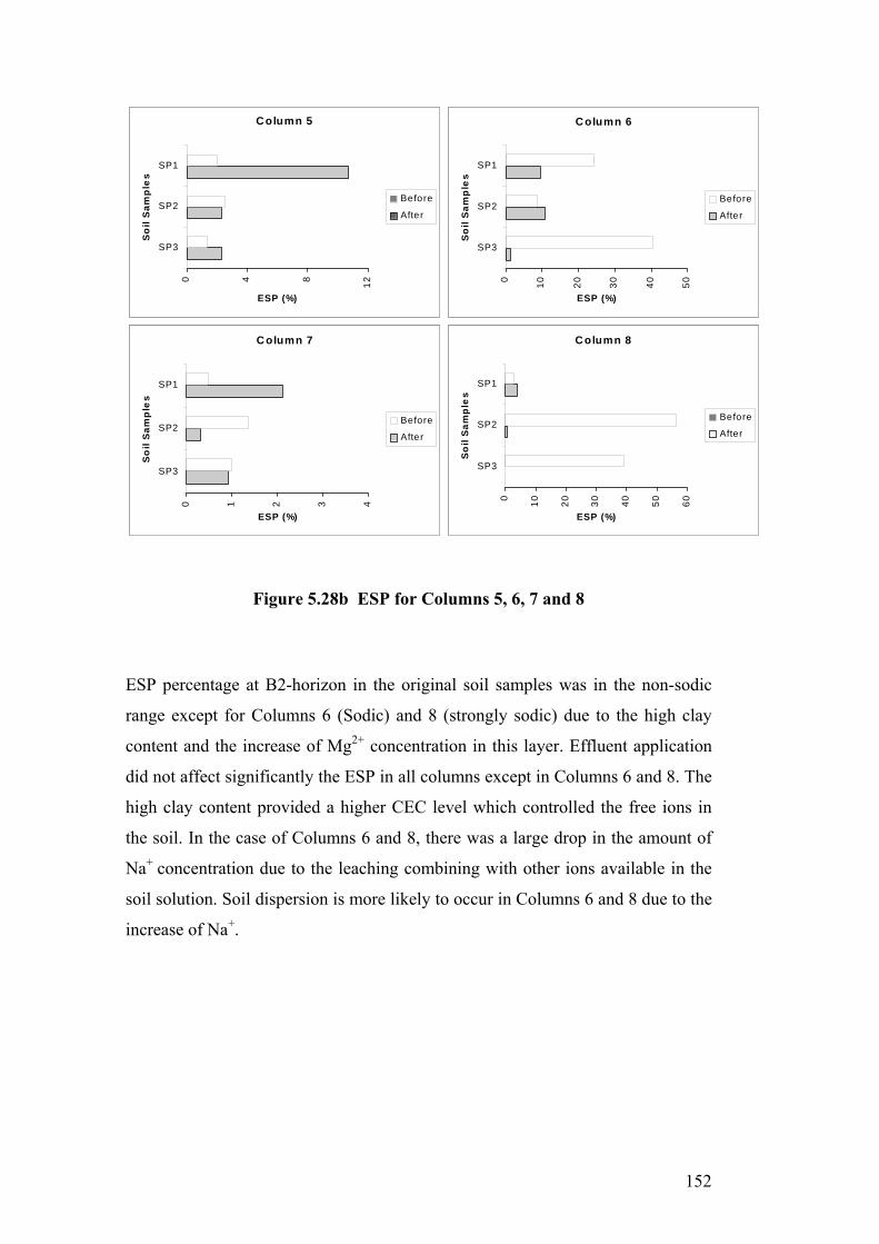
152

Figure 5.28b ESP for Columns 5, 6, 7 and 8

ESP percentage at B2-horizon in the original soil samples was in the non-sodic

range except for Columns 6 (Sodic) and 8 (strongly sodic) due to the high clay

content and the increase of Mg2+ concentration in this layer. Effluent application

did not affect significantly the ESP in all columns except in Columns 6 and 8. The

high clay content provided a higher CEC level which controlled the free ions in

the soil. In the case of Columns 6 and 8, there was a large drop in the amount of

Na+ concentration due to the leaching combining with other ions available in the

soil solution. Soil dispersion is more likely to occur in Columns 6 and 8 due to the

increase of Na+.

Column 5

0 4 8 12

SP3

SP2

SP1

So

il S

amp

les

ESP (%)

Before

After

C olumn 6

0 10 20 30 40 50

SP3

SP2

SP1

So

il S

amp

les

ESP (%)

Before

After

C olumn 7

0 1 2 3 4

SP3

SP2

SP1

So

il S

amp

les

ESP (%)

Before

After

C olumn 8

0 10 20 30 40 50 60

SP3

SP2

SP1

So

il S

amp

les

ESP (%)

Before

After

Column 5

0 4 8 12

SP3

SP2

SP1

So

il S

amp

les

ESP (%)

Before

After

C olumn 6

0 10 20 30 40 50

SP3

SP2

SP1

So

il S

amp

les

ESP (%)

Before

After

C olumn 7

0 1 2 3 4

SP3

SP2

SP1

So

il S

amp

les

ESP (%)

Before

After

C olumn 8

0 10 20 30 40 50 60

SP3

SP2

SP1

So

il S

amp

les

ESP (%)

Before

After

153

Figure 5.28c ESP for Columns 9, 10, 11 and 12

5.11 Effluent Analysis 5.11.1 Column 1 (Yellow Kurosol)

The previously discussed soil analysis contributed to knowledge of the soil

performance under effluent application. Also, the discussion covered the changes

which occurred as a result of effluent application. From Column 1 nine effluent

samples were collected from the different sampling points, with four samples

from the upper sampling point and five samples from the second sampling point

as reported in Appendix B, Table D1. The effluent samples were collected within

a period of 337 days.

The results indicated that the effluent poured into the soil columns was alkaline

(pH 8) and the pH for the effluent samples collected from the upper sampling

point was between 5.5 and 7.5. The highest pH value was recorded for the effluent

collected after 2 days and the lowest pH value was reported for the effluent

sample collected after 78 days. The effluent lost some alkalinity to the soil acidity.

C olumn 9

0 2 4 6 8 10

SP3

SP2

SP1

So

il S

amp

les

ESP (%)

Before

After

C olumn 10

0 2 4 6 8 10

1

2

3

So

il S

amp

les

ESP (%)

Before

After

C olumn 11

0 2 4 6 8 10

SP3

SP2

SP1

So

il S

amp

les

ESP (%)

Before

After

C olumn 12

0 2 4 6 8 10

SP3

SP2

SP1

So

il S

amp

les

ESP (%)

Before

After

C olumn 9

0 2 4 6 8 10

SP3

SP2

SP1

So

il S

amp

les

ESP (%)

Before

After

C olumn 10

0 2 4 6 8 10

1

2

3

So

il S

amp

les

ESP (%)

Before

After

C olumn 11

0 2 4 6 8 10

SP3

SP2

SP1

So

il S

amp

les

ESP (%)

Before

After

C olumn 12

0 2 4 6 8 10

SP3

SP2

SP1

So

il S

amp

les

ESP (%)

Before

After

154

This improvement reduced the toxicity conditions of the Al3+ present in the

subsurface and increased the microbial activity, which is necessary for

denitrifying the N reaching this horizon. The rise in soil pH is also considered a

positive indication for the increase of the microbial activity and P removal.

However, if the soil pH continues to increase this will be an adverse sign

indicating sodicity problems will occur in future.

Effluent samples collected from the upper sampling point indicated that the

average N removal was around 55%. The average N removal for the second

sampling point was 79%. The low N removal in the upper sampling point can be

attributed to the high nitrogen fixation level by the OM fraction and slow

microbial activity for the nitrification process. The soil ability to remove N

increased down the soil profile but did not reach the ultimate. Therefore, special

consideration should be given to the amount of nitrogen applied to the soil.

The amount of orthophosphate measured in the initial samples was low (1 mg/L)

and the removal was 92% in the upper sampling point. The P removal at the

second sampling point reached 98%. The high P removal is attributed to the low

level of P sorption capacity in the original soil. The effluent and soil test results

indicated that the Yellow Kurosol in Column 1 was capable of removing P from

the applied effluent.

Average EC in the effluent poured into the soil columns was 980 µS/cm, and the

EC reduction in the collected effluent samples from the upper sampling points

was low, reaching 48%, and at the second sampling point was 64%. The salts

accumulation will be a problem for the soil’s ability to treat effluent, due to the

increase of soil Na+ which will affect the exchangeable soil complex by replacing

the Ca2+ and Mg2+ with Na+.

The TCOD values varied in the collected effluent samples as reported in

Appendix B, Table D1. The removal at the upper sampling point was 71% and at

the second point was 89%. Most of the total COD was consumed by the microbial

activity in the biological mat which formed on the soil surface. The leaching of

COD to the lower depth was in a form of dissolved chemical oxygen demand

155

(DCOD). The leached DCOD was mostly consumed by microbial activity of the

denitrifying bacteria where suitable conditions for denitrification exist. The soil

removed most of the TCOD and continued to increase in pH with the increase in

the microbial activity.

The analysis for N, P, EC and TCOD removal are plotted against time for the first

and second sampling points in Figure 5.29 (A and B). The plotted figure showed

that the highest removal was phosphorus and the lowest was EC over 78 days at

the first sampling point. At the second sampling point, the highest removal by soil

was phosphorus and the lowest changed between EC and nitrogen after 250 days

of effluent application. The TCOD removal continued to rise with time. The

Yellow Kurosol provided sufficient removal of P and TCOD, and moderate ability

to remove N and EC.

Figure 5.29 (A and B) Contaminant removal by soils in Column 1

Effluent application was designed to be the same for all columns, but the effluent

ponding on the top surface of some columns controlled the effluent feeding and

sample collecton. Therefore, there are variations between the columns in relation

to the time required to achieve the wetting front for each sampling point as

discussed for each column. Additional information such as the column feeding

dates, the amount of effluent applied each time, the collection time of effluent

samples and the amount collected are reported in Appendix B, Table E1.

The soil column showed effluent ponding on the surface after 3 days. The total

amount of effluent required to saturate the soil column was 1470 mL. The wetting

Figure (A)

0

20

40

60

80

100

0 2 35 45 78

Days

Rem

oval

(%)Nitrogen

Phos.ECTCOD

Figure (B)

0

20

40

60

80

100

3 78 105 215 252

Days

Rem

oval

(%)Nitrogen

Phos.ECTCOD

156

front for the first sampling point at 110 mm was 3 days and the wetting time for

the second sampling point at 470 mm was 108 days and the third sampling point

was not reached during the experiment duration. Accordingly, Yellow Kurosol

has a slow effluent percolation rate and special attention should be given to the

amount of effluent applied.

In summary, Yellow Kurosol has a strong texture contrast between the different

horizons with strongly acid B-horizons. Also these soils have some unusual

chemical features, such as high Mg2+, Na+ and Al3+ content. The effluent

application improved alkalinity of the soil and affected the chemical

characteristics adversely in some cases and positively in others. The physico-

chemical characteristics indicated that the Yellow Kurosol has a high capability to

remove P and TCOD, and the soil has moderate capacity to remove N and soluble

salts. The mineralogy of the Kurosol soil with the information obtained from the

wetting points’ calculations showed that this soil has a low percolation rate.

Therefore, Yellow Kurosol is considered as having a moderate capacity to

renovate effluent and special consideration should be given in on-site treatment

system design. Design of the on-site system trenches should consider the

distribution of the discharged effluent over a larger subsurface area to ensure that

the applied effluent is transmitted by the soil. Table 5.3 summarises the findings

for the Yellow Kurosol soil.

157

Table 5.3 Summary of findings for the Yellow Kurosol (Column 1)

Before Effluent Application

After Effluent Application Effluent Treatment Capacity

• Acidic soil. • High organic matter

on A-horizon and lower at B-horizons.

• The dominant clay was kaolinite at the subsurface area with smectite presence.

• The CEC was in the range between 15 and 60 meq/100g.

• The individual cations analysis indicated that Ca and Mg were in the same level in the soil surface.

• Balanced ratio between Ca2+ and Mg2+ 1:1.

• Acidic soil which improved slightly after effluent application.

• Effluent application increased the OM at the subsurface layers.

• Less smectite presence due to the changes in the soil sampling position as a result of swell/shrink mechanisms.

• Almost the same CEC. • The increase of pH

improved the soils’ CEC.

• High salts content in the surface after effluent application.

• The soil has a high capacity to absorb effluent.

• The soil has low permeability (based on the accumulation of Cl- and observations).

• High nutrient absorption capacity.

• Effluent application increased Mg2+ at the subsurface layers and decreased Ca2+. Reduced soil fertility.

• There was a gradual increase in the ESP values in the soil.

The Yellow Kurosol soil has a moderate ability to treat effluent based on the following: • level of

pollutants removal from effluent (especially nitrogen)

• CEC and soil mineralogy

• low permeability, which requires special design consideration to help the soil to transmit effluent

• the change in the soil fertility and the increase of ESP

• the soluble salts accumulation

5.11.2 Column 2 (Hydrosol)

In Column 2, seven effluent samples were collected from the upper sampling

point within 321 days, four effluent samples were collected from the second

sampling point within 277 days and one sample of 30 mL was collected from the

third sampling point after 321 days (Appendix B, Table D2).

158


The pH of the seven effluent samples collected from the first or the upper

sampling point averaged 6.2. The pH values for the samples collected from the

second sampling point and the third averaged 5. The results for P, N, salts and

TCOD removal are plotted against time in Figure 5.30 (A and B). The removal

continued to increase at the upper sampling and reached 97% of the initial P input

after 321 days. The N removal reached 90% of the initial input of N. Also, the

removal of TCOD reached 90%. The EC removal at the upper sampling point was

low in the first four samples collected and started to rise slowly for the next three

samples. This slow EC removal is attributed to the unbalanced exchangeable

cations at A-horizon as shown in Figure 5.24. The soil has a good capacity to

renovate effluent through the profile with lower capacity to hold EC at A and B1-

horizons which increases to reach the maximum at B2-horizon due to the formed

barrier layer. Complete N, P, TCOD and EC removal is shown for the collected

samples from the B2-horizon. The effluent sample quality matched very well with

the soil evaluation, which means that the soil has a good ability to handle effluent

especially at the B2-horizon.

Additional data about soil performance under effluent application are presented in

Appendix B, Table E2. Ponding occurred directly after the effluent feeding and

then the effluent percolated slowly through the soil. The wetting front reached the

first sampling point at 120 mm after 18 days of effluent application. The wetting

front reached for the second sampling point at a distance of 480 mm after 147

days. The wetting time for the third sampling point at 780 mm was 323 days.

Figure (A)

0

20

40

60

80

100

0 43 77 96 120 194 277 321

Days

Rem

oval

(%)Nitrogen

Phos.

EC

TCOD

Figure (B)

90

92

94

96

98

100

128 157 186 275 321

Days

Rem

oval

(%)Nitrogen

Phos.

EC

TCOD

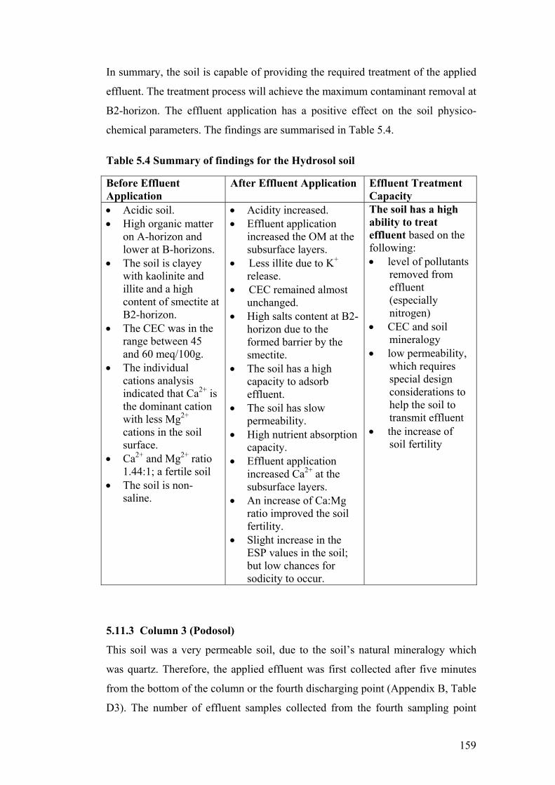
159

In summary, the soil is capable of providing the required treatment of the applied

effluent. The treatment process will achieve the maximum contaminant removal at

B2-horizon. The effluent application has a positive effect on the soil physico-

chemical parameters. The findings are summarised in Table 5.4.

Table 5.4 Summary of findings for the Hydrosol soil




on A-horizon and lower at B-horizons.

• The soil is clayey with kaolinite and illite and a high content of smectite at B2-horizon.


• The individual cations analysis indicated that Ca2+ is the dominant cation with less Mg2+ cations in the soil surface.

• Ca2+ and Mg2+ ratio 1.44:1; a fertile soil

• The soil is non-saline.

• Acidity increased. • Effluent application

increased the OM at the subsurface layers.

• Less illite due to K+ release.

• CEC remained almost unchanged.

• High salts content at B2-horizon due to the formed barrier by the smectite.

• The soil has a high capacity to adsorb effluent.

• The soil has slow permeability.


• Effluent application increased Ca2+ at the subsurface layers.

• An increase of Ca:Mg ratio improved the soil fertility.

• Slight increase in the ESP values in the soil; but low chances for sodicity to occur.

The soil has a high ability to treat effluent based on the following: • level of pollutants

removed from effluent (especially nitrogen)


• low permeability, which requires special design considerations to help the soil to transmit effluent

• the increase of soil fertility

5.11.3 Column 3 (Podosol)

This soil was a very permeable soil, due to the soil’s natural mineralogy which

was quartz. Therefore, the applied effluent was first collected after five minutes

from the bottom of the column or the fourth discharging point (Appendix B, Table

D3). The number of effluent samples collected from the fourth sampling point

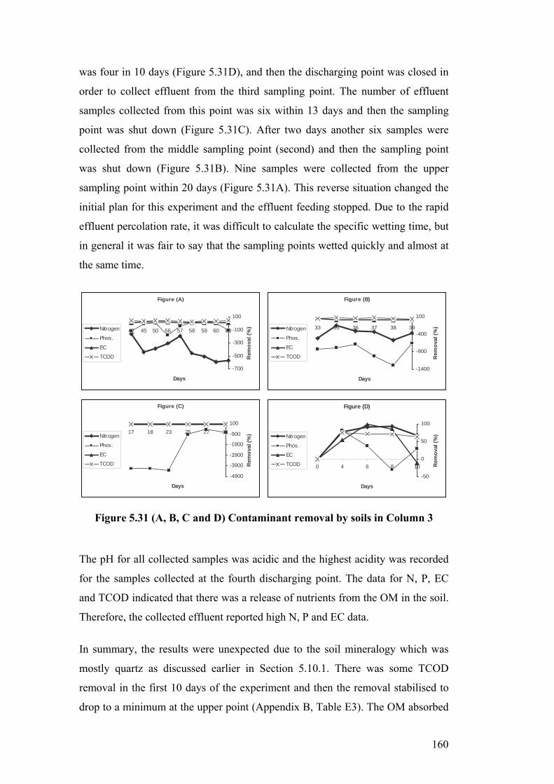
160

was four in 10 days (Figure 5.31D), and then the discharging point was closed in

order to collect effluent from the third sampling point. The number of effluent

samples collected from this point was six within 13 days and then the sampling

point was shut down (Figure 5.31C). After two days another six samples were

collected from the middle sampling point (second) and then the sampling point

was shut down (Figure 5.31B). Nine samples were collected from the upper

sampling point within 20 days (Figure 5.31A). This reverse situation changed the

initial plan for this experiment and the effluent feeding stopped. Due to the rapid

effluent percolation rate, it was difficult to calculate the specific wetting time, but

in general it was fair to say that the sampling points wetted quickly and almost at

the same time.

Figure 5.31 (A, B, C and D) Contaminant removal by soils in Column 3 The pH for all collected samples was acidic and the highest acidity was recorded

for the samples collected at the fourth discharging point. The data for N, P, EC

and TCOD indicated that there was a release of nutrients from the OM in the soil.

Therefore, the collected effluent reported high N, P and EC data.

In summary, the results were unexpected due to the soil mineralogy which was

mostly quartz as discussed earlier in Section 5.10.1. There was some TCOD

removal in the first 10 days of the experiment and then the removal stabilised to

drop to a minimum at the upper point (Appendix B, Table E3). The OM absorbed

Figure (A)

-700

-500

-300

-100

100

42 45 50 56 57 58 59 60 60

Days

Rem

oval

(%)Nitrogen

Phos.

EC

TCOD

Figure (B)

-1400

-900

-400

100

33 35 36 37 38 39

Days

Rem

oval

(%)Nitrogen

Phos.

EC

TCOD

Figure (C)

-4900

-3900

-2900

-1900

-900

10017 18 23 25 27 31

Days

Rem

oval

(%)Nitrogen

Phos.

EC

TCOD

Figure (D)

-50

0

50

100

0 4 6 8 10

Days

Rem

oval

(%)Nitrogen

Phos.

EC

TCOD

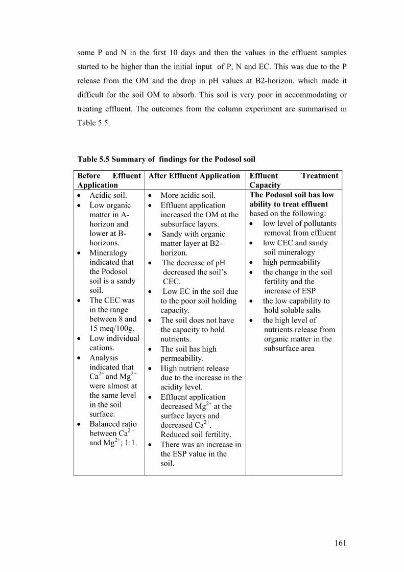
161

some P and N in the first 10 days and then the values in the effluent samples

started to be higher than the initial input of P, N and EC. This was due to the P

release from the OM and the drop in pH values at B2-horizon, which made it

difficult for the soil OM to absorb. This soil is very poor in accommodating or

treating effluent. The outcomes from the column experiment are summarised in

Table 5.5.

Table 5.5 Summary of findings for the Podosol soil



• Acidic soil. • Low organic

matter in A-horizon and lower at B-horizons.

• Mineralogy indicated that the Podosol soil is a sandy soil.


• Low individual cations.

• Analysis indicated that Ca2+ and Mg2+ were almost at the same level in the soil surface.

• Balanced ratio between Ca2+ and Mg2+; 1:1.

• More acidic soil. • Effluent application

increased the OM at the subsurface layers.

• Sandy with organic matter layer at B2-horizon.

• The decrease of pH decreased the soil’s CEC.

• Low EC in the soil due to the poor soil holding capacity.

• The soil does not have the capacity to hold nutrients.

• The soil has high permeability.

• High nutrient release due to the increase in the acidity level.

• Effluent application decreased Mg2+ at the surface layers and decreased Ca2+. Reduced soil fertility.

• There was an increase in the ESP value in the soil.

The Podosol soil has low ability to treat effluent based on the following: • low level of pollutants

removal from effluent • low CEC and sandy

soil mineralogy • high permeability • the change in the soil

fertility and the increase of ESP

• the low capability to hold soluble salts

• the high level of nutrients release from organic matter in the subsurface area

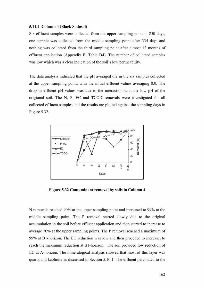
162

5.11.4 Column 4 (Black Sodosol)

Six effluent samples were collected from the upper sampling point in 250 days,

one sample was collected from the middle sampling point after 334 days and

nothing was collected from the third sampling point after almost 12 months of

effluent application (Appendix B, Table D4). The number of collected samples

was low which was a clear indication of the soil’s low permeability.

The data analysis indicated that the pH averaged 6.2 in the six samples collected

at the upper sampling point, with the initial effluent values averaging 8.0. The

drop in effluent pH values was due to the interaction with the low pH of the

origional soil. The N, P, EC and TCOD removals were investigated for all

collected effluent samples and the results are plotted against the sampling days in

Figure 5.32.

0

20

40

60

80

100

0 2 6 43 75 82 250

334b

Days

Rem

oval

(%)Nitrogen

Phos.

EC

TCOD

Figure 5.32 Contaminant removal by soils in Column 4

N removals reached 90% at the upper sampling point and increased to 99% at the

middle sampling point. The P removal started slowly due to the original

accumulation in the soil before effluent application and then started to increase to

average 70% at the upper sampling points. The P removal reached a maximum of

99% at B1-horizon. The EC reduction was low and then proceded to increase, to

reach the maximum reduction at B1-horizon. The soil provided low reduction of

EC at A-horizon. The mineralogical analysis showed that most of this layer was

quartz and kaolinite as discussed in Section 5.10.1. The effluent percolated to the

163

lower horizon where the soil contained smectite which formed a barrier as

discussed in Section 5.10.1 and the reduction of EC was almost completed.

Progressive ponding started to occur after three days. The wetting time for the

first sampling point at 80 mm occurred after 2 days and the wetting front for the

second sampling point at 440 mm soil depth occurred after 330 days (Appendix B,

Table E4).

In summary, based on the physico-chemical parameters, this soil will be suitable

to provide the required treatment for the effluent especially in the lower horizon.

The chance of sodicity is very low in the short term. The fertility of the soil is

expected to decrease over time. The soil has a low permeability level and special

consideration should be given to the design of the on-site treatment facility. Table

5.6 summarises the outcomes.

164

Table 5.6 Summary of findings for the Black Sodosol soil


After Effluent Application

Effluent Treatment Capacity


in A-horizon and B2-horizon and lower at B1-horizon.

• The soil has a high quartz content at A and B1-horizons. Kaolinite and smectite clay were detected in the soil samples.


• The individual cations analysis indicated that Ca2+ and Mg2+ were in the same level in the soil surface.

• Balanced ratio between Ca2+ and Mg2+; 1:1. Soil fertile at the surface, low fertility at B-horizons due to the increase of ESP.

• pH over 6 at A and B1-horizons and acidic soil at B2-horizon.

• Effluent application increased the OM at A and B1-horizon subsurface layers.

• Smectite/swelling occurred.

• Increase of CEC especially at B2-horizons.

• The increase of pH improved the biological activity in the soil.

• High salts content in the subsurface area.

• The soil has a high capacity to adsorb nutrients at the upper level.

• The soil has low permeability.

• High exchangeable cations in the soil.


• There was a gradual increase in ESP in the soil.

The Black Sodosol soil has a high ability to treat effluent based on the following: • high level of pollutants

removal • high CEC level and soil

mineralogy • low permeability,

which requires especial design consideration to help the soil to transmit effluent



5.11.5 Column 5 (Red Dermosol)

Eight effluent samples were collected from the upper sampling point in 292 days

and the pH range was between 6.6 and 7.7. N removal (68%) and P (47%)

removal was low. This was due to the low OM in this layer and the mineralogy of

the column as discussed in Section 5.10. Due to the low OM available for N

165

uptake, it is important to note that the OM almost reached the maximum capacity

to uptake nutrients from effluent. The soil's high sodicity was reflected in the

collected effluent samples’ pH and continued effluent application would make the

pH rise. Figure 5.3 shows the different removal ratios for N, P, EC and TCOD.

The figure also shows that there was a high removal in the first three days and

then continued to decrease until it stabilised after 218 days and started to increase

slowly but was still low. This means that when the OM and the soil started to

stabilise, the OM has more capacity for uptake of the added nutrients.

0

20

40

60

80

100

0 3 7 28 34 40 52 218

292

Days

Rem

oval

(%)Nitrogen

Phos.

EC

TCOD


The wetting front for the first sampling point at 100 mm soil depth was reached

after two days and for the second sampling point at soil depth 460 mm after 317

days. There was no effluent samples collected from the third sampling point for

the duration of the column experiment (Appendix B, Table E5).

In summary, the Red Dermosol soil type has a low capacity to treat or transmit

effluent. This soil has a high sodicity associated with low fertility. The areas with

such soil require special attention. Table 5.7 summarises the findings for the Red

Dermosol soil before and after effluent application.

166

Table 5.7 Summary of findings for the Red Dermosol Soil




• High organic matter on A and B2-horizons and lower at B1-horizon.

• Sandy soil with low clay content in A and B1-horizon.

• The CEC was between 10 and 18 meq/100g.

• The individual cations analysis indicated that Ca2+ and Mg2+ were in the same level in the soil surface.

• Almost balanced ratio between Ca2+ and Mg2+; 1:1.

• Effluent application slightly increased the OM in all layers.

• The decrease of pH decreased slightly the soils’ CEC at A-horizon.

• High salts content in all the soil layers

• The soil has a low capacity to adsorb effluent.




The Red Dermosol soil has a low ability to treat effluent based on the following: • low level of

pollutants removal from effluent

• low CEC and sandy mineralogy

• high permeability which requires special design consideration

• the Ca:Mg ratio decreased due to the effluent application

• increase of ESP • the soluble salts

accumulation

5.11.6 Column 6 (Brown Kurosol)

Five effluent samples were collected from the upper effluent sampling point in

269 days; one sample from the second sampling point after 98 days and one

sample from the third sampling point after 105 days (Appendix B, Table D6). The

pH range for the samples from the upper sampling point was between 7.01 to 7.45.

The removal of N, P, EC and TCOD are plotted against time at Figure 5.34. It

shows low removal for the different sampling periods. The removal of P and EC

decreased with time. This was due to the low exchange capacity provided in this

soil type as discussed in Section 5.10.3. This soil has low capacity to handle or

treat effluent.

167

0

20

40

60

80

100

0 78 85 95 115

274

Days

Rem

oval

(%)Nitrogen

Phos.

EC

TCOD


The wetting time for the first sampling point was 2 days for 110mm. The wetting

time for the second sampling point was 101 days for 470 mm and finally the

wetting time for the third sampling point was 199 days for 770 mm. (Appendix B,

Table E6).

In summary, the soil physico-chemical data indicated that this soil has a low

capacity to remove contaminants from effluent. The effluent application indicated

that the removal of contaminants by soil was low as a result of low CEC level

available due to low clay content as shown in Figure 5.17b. Also, this soil is

extremely acidic which has an adverse impact on the biological activity which is

necessary for contaminants removal as discussed in Section 5.10.4. The Ca:Mg

ratio indicated that this soil has a low fertility level before and after effluent

application due to imbalance between Ca2+ and Mg2+. ESP was high before

effluent application due to the imbalance in the cations concentration in the soil

horizons. Effluent application increased the Mg2+ accumulation through the soil

profile which inhibited the increase of Na+ in the at B2-horizon. The increase of

Mg2+ and the decrease of Na+ affected the soil ESP positively. As a result, the soil

changed from strongly-sodic to non-sodic at the B2-horizon. This soil can be

classified as having a low capacity to handle or treat effluent. Table 5.8

summarises the findings for the soil column.

168

Table 5.8 Summary of findings for the Brown Kurosol Soil




• Low organic matter in A-horizon and lower at B-horizons.

• Sandy soil with kaolinite.

• The CEC was between 2 and 13 meq/100g.

• Low individual exchangeable cations and low fertility.

• High ESP (sodic).

• Effluent application increased the OM at A and B1-horizons.

• The increase of pH improved the soils’ CEC.


• The soil has a low capacity to adsorb effluent.


• Lower exchangeable cations.

• Lower fertility. • Lower ESP.

The Brown Kurosol soil has low ability to treat effluent based on the following: • low level of pollutants

removal from effluent • low CEC and sandy

soil mineralogy • moderate permeability • the change in the soil

fertility and the increase of ESP


• the soil sodicity

5.11.7 Column 7 (Brown Vertosol)

The results show that a total of 12 effluent samples were collected from the three

sampling points (Appendix B, Table D7). Eight effluent samples were collected

from the upper sampling point, four from the second point and two samples from

the third sampling point. Figure 5.35 (A and B) shows that the average removals

in the effluent samples at the upper sampling point were N (78%) P (78%), EC

(70%) and TCOD (90%). These removals were considered in the medium range.

This level of removal is attributed to the high quartz content and low kaolinite

content which provided a low CEC. Also, the deposition of OM in the lower

horizons disturbed the soil structure at A-horizon.

The average removals at B1-horizon increased to reach N (89%), P (75%), EC

(81%) and TCOD (95%). The average removals at B2-horizons increased to reach

N (99%), P (91%), EC (98%), and TCOD (98%). The contaminants removals

increased gradually to reach the maximum at B2-horizon as a result of increase of

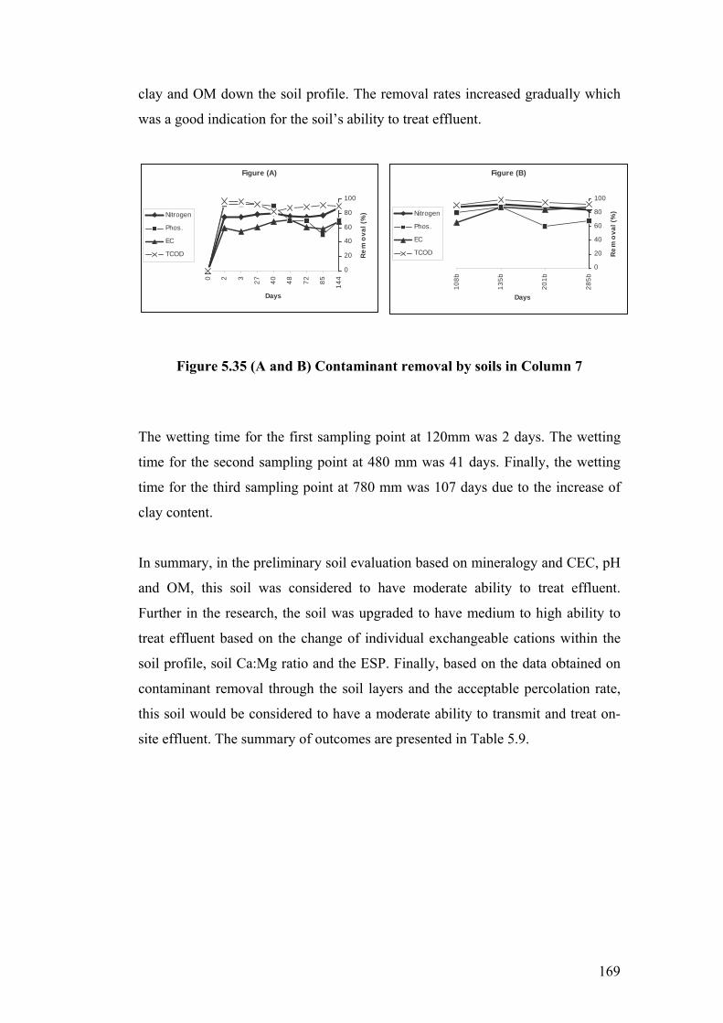
169

clay and OM down the soil profile. The removal rates increased gradually which

was a good indication for the soil’s ability to treat effluent.


The wetting time for the first sampling point at 120mm was 2 days. The wetting

time for the second sampling point at 480 mm was 41 days. Finally, the wetting

time for the third sampling point at 780 mm was 107 days due to the increase of

clay content.

In summary, in the preliminary soil evaluation based on mineralogy and CEC, pH

and OM, this soil was considered to have moderate ability to treat effluent.

Further in the research, the soil was upgraded to have medium to high ability to

treat effluent based on the change of individual exchangeable cations within the

soil profile, soil Ca:Mg ratio and the ESP. Finally, based on the data obtained on

contaminant removal through the soil layers and the acceptable percolation rate,

this soil would be considered to have a moderate ability to transmit and treat on-

site effluent. The summary of outcomes are presented in Table 5.9.

Figure (A)

0

20

40

60

80

1000 2 3 27 40 48 72 85 144

Days

Re

mo

val (

%)Nitrogen

Phos.

EC

TCOD

Figure (B)

0

20

40

60

80

100

108b

135b

201b

285b

Days

Re

mo

val (

%)Nitrogen

Phos.

EC

TCOD

170

Table 5.9 Summary of findings for Brown Vertosol Soil



• Low OM in A-horizon increased down the soil profile.

• Sandy soil with increasing kaolinite content down the soil profile.

• The CEC was around 30 meq/100g for all horizons.

• High exchangeable cations lower down the soil profile.

• Fertile at the surface, lower fertility down the soil profile.

• Effluent application increased the OM down the soil profile.

• High salts content in the surface and subsurface after effluent application.

• The soil has a moderate capacity to absorb effluent.

• The soil has average permeability.

• A moderate nutrient absorption capacity especially at A-horizon.

• Effluent application decreased the Mg2+ cations at the subsurface layers and decreased Ca2+.

• Dispersion on the surface is expected in the future due to the increase of soluble salts especially at A and B1-horizons and the increase of ESP.

The Brown Vertosol soil has a moderate ability to treat effluent based on the following: • level of pollutants

removal from effluent (especially nitrogen)


• average permeability

• the change in the soil fertility

• the increase of ESP


5.11.8 Column 8 (Brown Dermosol)

Nine effluent samples were collected from the upper sampling point in 269 days.

The pH ranged between 6.2 and 7, the range of removals of P, N, EC and TCOD

were 75-87%, 79-92%, 67 to 97% and 88 to 95% respectively (Appendix B, Table

D8). The results show that there was a high removal of contaminants by the soil in

the A-horizon. Five effluent samples were collected from the second sampling

point in 337 days and the amount collected was 460 mL. The removals ranges

were 87-94% (P), 91-99% (N), 91-97% (EC) and 93-96% (TCOD). The removal

capacity was higher at the second sampling point than the first sampling point but

there was a decrease in the effluent pH. A small sample was collected from the

third sampling point after 337 days. The sample characterisation indicated a lower

pH and the removal rates were almost the same as the middle sampling point

results. The removal percentage for the collected samples is plotted in Figure 5.36

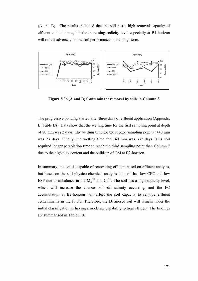
171

(A and B). The results indicated that the soil has a high removal capacity of

effluent contaminants, but the increasing sodicity level especially at B1-horizon

will reflect adversely on the soil performance in the long- term.


The progressive ponding started after three days of effluent application (Appendix

B, Table E8). Data show that the wetting time for the first sampling point at depth

of 80 mm was 2 days. The wetting time for the second sampling point at 440 mm

was 73 days. Finally, the wetting time for 740 mm was 337 days. This soil

required longer percolation time to reach the third sampling point than Column 7

due to the high clay content and the build-up of OM at B2-horizon.

In summary, the soil is capable of renovating effluent based on effluent analysis,

but based on the soil physico-chemical analysis this soil has low CEC and low

ESP due to imbalance in the Mg2+ and Ca2+. The soil has a high sodicity level,

which will increase the chances of soil salinity occurring, and the EC

accumulation at B2-horizon will affect the soil capacity to remove effluent

contaminants in the future. Therefore, the Dermosol soil will remain under the

initial classification as having a moderate capability to treat effluent. The findings

are summarised in Table 5.10.

Figure (A)

0

20

40

60

80

100

0 2 8 40 63 85 170

231

269

307

Days

Rem

oval

(%)Nitrogen

Phos.

EC

TCOD

Figure (B)

80

85

90

95

100

130b

180b

220b

292b

337b

337c

Days

Rem

oval

(%)Nitrogen

Phos.

EC

TCOD

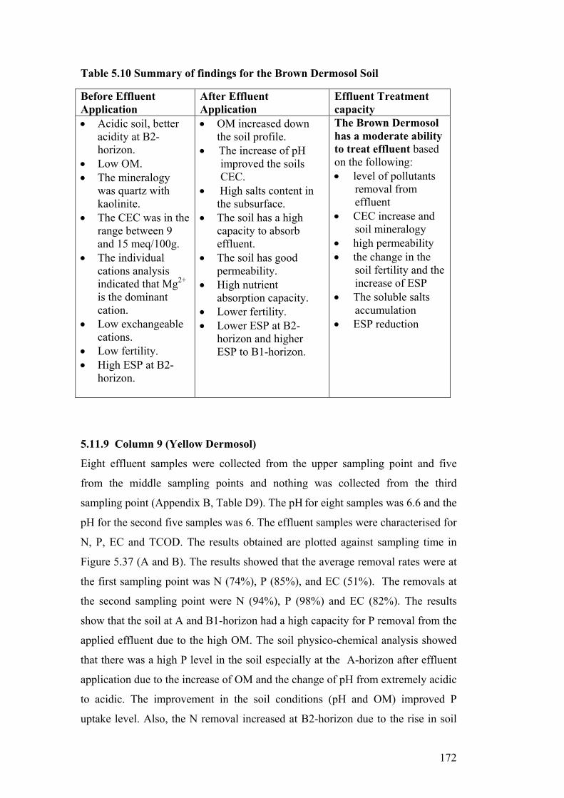
172

Table 5.10 Summary of findings for the Brown Dermosol Soil



Effluent Treatment capacity

• Acidic soil, better acidity at B2-horizon.

• Low OM. • The mineralogy

was quartz with kaolinite.


• The individual cations analysis indicated that Mg2+ is the dominant cation.

• Low exchangeable cations.

• Low fertility. • High ESP at B2-

horizon.

• OM increased down the soil profile.

• The increase of pH improved the soils CEC.

• High salts content in the subsurface.

• The soil has a high capacity to absorb effluent.

• The soil has good permeability.


• Lower fertility. • Lower ESP at B2-

horizon and higher ESP to B1-horizon.

The Brown Dermosol has a moderate ability to treat effluent based on the following: • level of pollutants

removal from effluent

• CEC increase and soil mineralogy

• high permeability • the change in the

soil fertility and the increase of ESP

• The soluble salts accumulation

• ESP reduction

5.11.9 Column 9 (Yellow Dermosol)

Eight effluent samples were collected from the upper sampling point and five

from the middle sampling points and nothing was collected from the third

sampling point (Appendix B, Table D9). The pH for eight samples was 6.6 and the

pH for the second five samples was 6. The effluent samples were characterised for

N, P, EC and TCOD. The results obtained are plotted against sampling time in

Figure 5.37 (A and B). The results showed that the average removal rates were at

the first sampling point was N (74%), P (85%), and EC (51%). The removals at

the second sampling point were N (94%), P (98%) and EC (82%). The results

show that the soil at A and B1-horizon had a high capacity for P removal from the

applied effluent due to the high OM. The soil physico-chemical analysis showed

that there was a high P level in the soil especially at the A-horizon after effluent

application due to the increase of OM and the change of pH from extremely acidic

to acidic. The improvement in the soil conditions (pH and OM) improved P

uptake level. Also, the N removal increased at B2-horizon due to the rise in soil

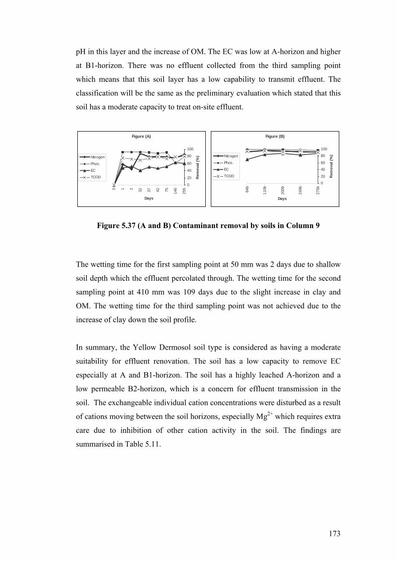
173

pH in this layer and the increase of OM. The EC was low at A-horizon and higher

at B1-horizon. There was no effluent collected from the third sampling point

which means that this soil layer has a low capability to transmit effluent. The

classification will be the same as the preliminary evaluation which stated that this

soil has a moderate capacity to treat on-site effluent.


The wetting time for the first sampling point at 50 mm was 2 days due to shallow

soil depth which the effluent percolated through. The wetting time for the second

sampling point at 410 mm was 109 days due to the slight increase in clay and

OM. The wetting time for the third sampling point was not achieved due to the

increase of clay down the soil profile.

In summary, the Yellow Dermosol soil type is considered as having a moderate

suitability for effluent renovation. The soil has a low capacity to remove EC

especially at A and B1-horizon. The soil has a highly leached A-horizon and a

low permeable B2-horizon, which is a concern for effluent transmission in the

soil. The exchangeable individual cation concentrations were disturbed as a result

of cations moving between the soil horizons, especially Mg2+ which requires extra

care due to inhibition of other cation activity in the soil. The findings are

summarised in Table 5.11.

Figure (A)

0

20

40

60

80

100

0 1 2 32 37 42 75 146

255

Days R

emov

al (%

)Nitrogen

Phos.

EC

TCOD

Figure (B)

0

20

40

60

80

100

84b

110b

200b

249b

275b

Days

Rem

oval

(%)Nitrogen

Phos.

EC

TCOD

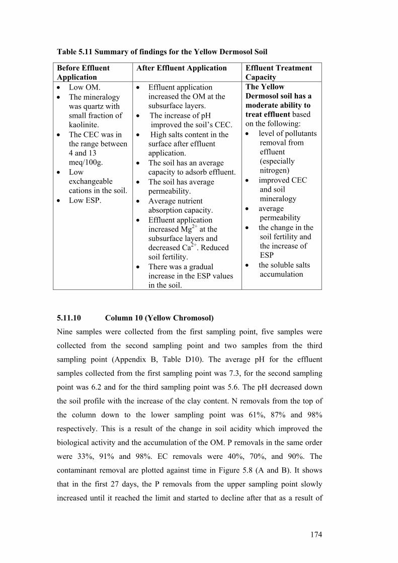
174

Table 5.11 Summary of findings for the Yellow Dermosol Soil



• Low OM. • The mineralogy

was quartz with small fraction of kaolinite.


• Low exchangeable cations in the soil.

• Low ESP.

• Effluent application increased the OM at the subsurface layers.

• The increase of pH improved the soil’s CEC.


• The soil has an average capacity to adsorb effluent.

• The soil has average permeability.

• Average nutrient absorption capacity.



The Yellow Dermosol soil has a moderate ability to treat effluent based on the following: • level of pollutants

removal from effluent (especially nitrogen)

• improved CEC and soil mineralogy

• average permeability



5.11.10 Column 10 (Yellow Chromosol)

Nine samples were collected from the first sampling point, five samples were

collected from the second sampling point and two samples from the third

sampling point (Appendix B, Table D10). The average pH for the effluent

samples collected from the first sampling point was 7.3, for the second sampling

point was 6.2 and for the third sampling point was 5.6. The pH decreased down

the soil profile with the increase of the clay content. N removals from the top of

the column down to the lower sampling point was 61%, 87% and 98%

respectively. This is a result of the change in soil acidity which improved the

biological activity and the accumulation of the OM. P removals in the same order

were 33%, 91% and 98%. EC removals were 40%, 70%, and 90%. The

contaminant removal are plotted against time in Figure 5.8 (A and B). It shows

that in the first 27 days, the P removals from the upper sampling point slowly

increased until it reached the limit and started to decline after that as a result of

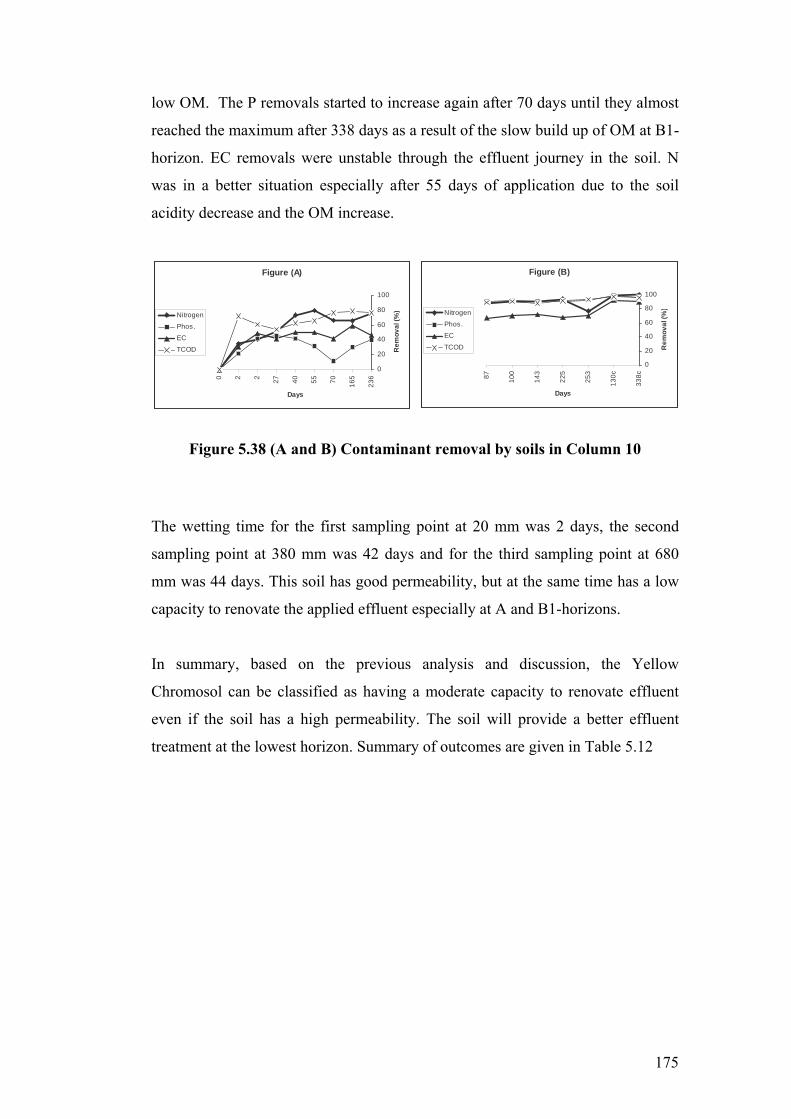
175

low OM. The P removals started to increase again after 70 days until they almost

reached the maximum after 338 days as a result of the slow build up of OM at B1-

horizon. EC removals were unstable through the effluent journey in the soil. N

was in a better situation especially after 55 days of application due to the soil

acidity decrease and the OM increase.


The wetting time for the first sampling point at 20 mm was 2 days, the second

sampling point at 380 mm was 42 days and for the third sampling point at 680

mm was 44 days. This soil has good permeability, but at the same time has a low

capacity to renovate the applied effluent especially at A and B1-horizons.

In summary, based on the previous analysis and discussion, the Yellow

Chromosol can be classified as having a moderate capacity to renovate effluent

even if the soil has a high permeability. The soil will provide a better effluent

treatment at the lowest horizon. Summary of outcomes are given in Table 5.12

Figure (A)

0

20

40

60

80

100

0 2 2 27 40 55 70 165

236

Days R

emov

al (%

)Nitrogen

Phos.

EC

TCOD

Figure (B)

0

20

40

60

80

100

87 100

143

225

253

130c

338c

Days

Rem

oval

(%)Nitrogen

Phos.

EC

TCOD

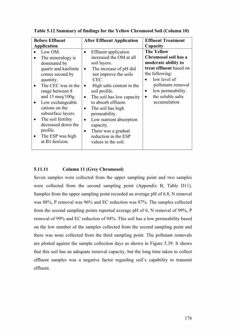
176

Table 5.12 Summary of findings for the Yellow Chromosol Soil (Column 10)



• Low OM. • The mineralogy is

dominated by quartz and kaolinite comes second by quantity.


• Low exchangeable cations on the subsurface layers.

• The soil fertility decreased down the profile.

• The ESP was high at B1-horizon.

• Effluent application increased the OM at all soil layers.

• The increase of pH did not improve the soils CEC.

• High salts content in the soil profile.

• The soil has low capacity to absorb effluent.


• Low nutrient absorption capacity.

• There was a gradual reduction in the ESP values in the soil.

The Yellow Chromosol soil has a moderate ability to treat effluent based on the following: • low level of

pollutants removal • low permeability. • the soluble salts

accumulation

5.11.11 Column 11 (Grey Chromosol)

Seven samples were collected from the upper sampling point and two samples

were collected from the second sampling point (Appendix B, Table D11).

Samples from the upper sampling point recorded an average pH of 6.8, N removal

was 88%, P removal was 96% and EC reduction was 87%. The samples collected

from the second sampling points reported average pH of 6, N removal of 99%, P

removal of 99% and EC reduction of 94%. This soil has a low permeability based

on the low number of the samples collected from the second sampling point and

there was none collected from the third sampling point. The pollutant removals

are plotted against the sample collection days as shown in Figure 5.39. It shows

that this soil has an adequate removal capacity, but the long time taken to collect

effluent samples was a negative factor regarding soil’s capability to transmit

effluent.

177

0

20

40

60

80

100

0 85 110

130

182

243

286

318

240

330

Days

Rem

oval

(%)Nitrogen

Phos.

EC

TCOD

Figure 5.39 Contaminant removal by soils in Columns 11

The wetting time for the first sampling point at 60 mm was 109 days, the second

sampling point at 420 mm was 248 days due to the significant increase in the clay

content down the soil profile. There was no effluent samples collected from the

third sampling point at 720 mm during the time of the experiment (Appendix B,

Table E10).

In summary, the analysis indicated that the effluent affected the original soil CEC

adversely at A and B1-horizon. The CEC at B2-horizon stayed almost the same as

the original. The soil has low CEC, especially in the lower B2-horizon and the

effluent increased the ESP level at A-horizon and reduced the fertility level. The

soil at A and B-horizons relies too much on the OM contribution to the level of

CEC. The soil at B-horizon was controlled by the CEC supplied by the clay in this

layer. Effluent contaminant removals were high at A-horizon and reached almost

the ultimate level at B-horizons. The soil has a low permeability level. Therefore,

this soil can be classified as a having moderate suitability for effluent renovation

due to the low permeability and the progressive increase in the ESP level in the

soil as a result of continuous effluent application. Summary of findings for the

Grey Chromosol is presented in Table 5.13.

178

Table 5.13 Summary of findings for the Grey Chromosol Soil



• Low OM at A-horizon and higher at B2-horizon.

• The dominant clay was kaolinite at B2-horizon with small fraction of illite.


• The individual cations analysis indicated that Ca2+ and Mg2+ were almost in the same level in the soil surface.

• Exchangeable cations and fertility decreased with depth.

• ESP increased with depth.

• Effluent application increased the OM.

• The increase of OM improved the soil’s pH.

• High salts content in the soil profile.

• The soil has a high capacity to adsorb effluent.



• Fertility and exchangeable cations decreased.

• ESP increased on the surface.

The Grey Chromosol soil has a moderate ability to treat effluent based on the following: • level of pollutants


• change in CEC and soil mineralogy

• low permeability, which requires special design considerations

• the change in the soil fertility and the increase of ESP on the surface; the soil could disperse

• soluble salts accumulation

5.11.12 Column 12 (Red Kandosol)

Eleven samples were collected from the upper sampling point with average pH of

7.3, five samples were collected from the second sampling point with average pH

of 6.1, three samples were collected from the third sampling point with average

pH of 5.5 and two samples were collected from the bottom of the soil column with

average pH of 4.9 (Appendix B, Table D12).

The contaminant removals were varied within the soil horizons. The removals at

the upper sampling points were P (90%), N (75%) and EC (62%). The removals at

the second sampling point were P (90%), N (85%) and EC (80%). The removals

at the third sampling point were P (95%), N (97%) and EC (92%). Finally, the

removals at the fourth sampling point or the discharging point at the bottom of the

column were P (90%), N (92%) and EC (96%). The removals are plotted against

179

time in Figure 5.40 (A, B and C). The soil performed well from the beginning for

P removal. Other contaminant removals were less than for P and the only concern

was the EC reduction at the upper sampling point. The removals improved for the

samples collected from the second sampling point and continued to improve to

reach the maximum at the third sampling point due to the increase of clay content

down the soil profile. The removals in the samples collected from the fourth

sampling point were slightly less than the removals of the third sampling point,

which could be due to the low effluent acidity at the bottom.

Figure 5.40 (A, B and C) Contaminant removal by soils in Column 12

The wetting time for the first sampling point at 80 mm was 2 days, for the second

sampling point at 440 mm was 76 days, the third sampling point at 740 mm was

144 days and the wetting time for the fourth sampling point at 830 mm was 144

days (Appendix B, Table E12).

In summary, the Red Kandosol was classified previously as having a moderate-

high suitability for effluent renovation. The soil classification was upgraded to a

high suitablility for on-site effluent renovation. This classification was based on

Figure (A)

0

20

40

60

80

100

0 2 3 5 27 35 55 77 135

185

249

266

Days

Rem

oval

(%)Nitrogen

Phos.

EC

TCOD

Figure (B)

0

20

40

60

80

100

102

135

185

149

232

Days

Rem

oval

(%)Nitrogen

Phos.

EC

TCOD

Figure (C)

80

85

90

95

100

137

240

338

Days

Rem

oval

(%)Nitrogen

Phos.

EC

TCOD

180

good permeability and a high renovation capacity especially at the lower horizons.

The soil requires special attention due to the decrease in the fertility and the

progressive increase of the ESP or the soil sodicity, in long-term effluent

application. Summary of findings is reported in Table 5.14.

Table 5.14 Findings for the Red Kandosol Soil



• Low OM at A-horizon and higher at B-horizon.

• The dominant clay was kaolinite and illite.


• The individual cations analysis indicated that Mg2+ is the dominant cation.

• Effluent application increased the OM at A and B1-horizons.

• The increase of OM improved the soils pH.

• High salts content on the surface.



• Effluent application decreased Mg2+ at the subsurface layers and decreased Ca2+. Reduced soil fertility

• ESP increased at A-horizons.

The Yellow Kandosol soil has a high ability to treat effluent based on the following: • level of pollutants



• low permeability which requires especial design considerations to help the soil to transmit effluent



5.12 Conclusions The undisturbed soil column experiment was an important stage in the research.

This stage provided knowledge about the actual soil performance under effluent

application. The experimental design were the major factors in the success of the

column experiment. The undisturbed soil cores were critical for this study.

In general, the soils were varied in the treatment level provided based on physico-

chemical characteristics. The soils considered to have a low capacity to treat

effluent were Podosol, Red Dermosol and Brown Kurosol. The soil types

181

considered to have a moderate treatment capacity were Yellow Kurosol, Brown

Vertosol, Brown Dermosol, Yellow Dermosol, Yellow Chromosol and Grey

Chromosol. Finally, soil types considered having a high treatment capacity were

Hydrosol, Black Sodosol and Red Kandosol.

182

Chapter 6 Data Analysis and Validation

6.1 Overview The failure of a soil to transmit or treat discharged effluent can lead to serious

health and environmental problems. Evaluating soils based on their physico-

chemical characteristics prior to the installation of an on-site sewage treatment

system will reduce such problems.

Each soil order has a different capacity to treat and transmit effluent. The soil

evaluation based on CEC and pH measurements increased the knowledge about

the soil’s physico-chemical characteristics. The preliminary soil evaluation which

was based mainly on the soil’s CEC level was not sufficient due to the limited

number of physico-chemical parameters involved in the evaluation. There were

another five soil physico-chemical parameters not included in the soil evaluation

which are EC, Cl-, phosphorus as PO43-, nitrogen as NH3-N and OM. As a result

there was a large amount of data generated, which made it difficult to manipulate

or evaluate. This problem was overcome by using chemometrics methods and

multi-criteria decision-making analysis for deriving a better understanding of the

soils’ behaviour.

The data obtained from the laboratory columns study also helped investigate

another important concept in relation to effluent disposal to the soil. Frequent or

continuous sewage effluent application to the soil results in the growth of a

biological layer (clogging mat) on the soil surface. In general, this mat is formed

at the surface of filtration in the soil. It acts as a filter, which removes solid

particles carried by the effluent. The clogging mat develops at a rate dependent on

the effluent load. The thickness of the mat is dependent on the effluent quality,

soil type, and the environmental conditions such as weather, rainfall and depth to

the water table. The infiltrative rate slowly decreases over time due to the

formation of the clogging mat. The long-term acceptance rate (LTAR) for the soil

is defined as the average infiltrative rate through the clogging layer. The LTAR

varies between different soil types and is usually reached after a period of

continuous effluent application. The results discussed in relation to the column

experiment study (Chapter 5) together with the outcomes from the soil

183

characterization (Chapter 4) were used for determining the LTAR for twelve soil

types which were selected for the column experiment.

6.2 Evaluation Based on Soil’s CEC The assumptions used for classifying the sites on their ability to treat effluent

were based on the CEC level available at the B-horizon of each site. The

following assumptions were used to evaluate the soil’s ability to renovate on-site

effluent:

• Soil mineralogy dominated mainly by quartz and kaolinite and with CEC

values between 0 and 20 meq/100g was considered to have a low ability to

treat effluent.

• Soil mineralogy of quartz, kaolinite and small fraction of illite and CEC

values between 20 and 50 meq/100g was considered to have a moderate

ability to treat effluent.

• Soil mineralogy of quartz, kaolinite and smectite, with CEC values higher

than 50 meq/100g was considered to have a high ability to treat on-site

effluent.

Based on the above assumptions, 33% of the investigated sites were considered as

having a low ability to treat on-site effluent, 42% of the sites to have a moderate

ability and 25% of the investigated sites to have a high ability to treat effluent. A

summary of the results are reported in Table 6.1.

184

Table 6.1 Soil classification based on CEC level available on each site.

Site Number Soil Type Ability Classification

1, 8, 11, 13, 14, 15,

29, 30, 32 and 39

Yellow Dermosol

5 and 10 Red Dermosol

23 Grey Dermosol

12 Bleached-Leptic Tenosol

38 and 41 Rudosol

Low

2, 3 and 4 Grey Chromosol

6 and 48 Brown Chromosol

9 Yellow Chromosol

7 and 42 Grey Kurosol

37 Brown Kurosol

16 and 46 Brown Vertosol

20 and 35 Red Vertosol

36 and 33 Red Sodosol

31 Grey Sodosol

24, 43 and 44 Yellow Sodosol

45 Spolic Anthroposol

Moderate

17, 25, 26 and 27 Red Kandosol

18, 19, 21, 22 and 28 Yellow Kandosol

34 and 40 Brown Kandosol

47 Red Dermosol

High

In addition to the classification reported in Table 6.1, the data analysis of the

preliminary and detailed investigation stages as discussed in Chapter 4 showed the

following:

• The soils in the investigated sites are acidic;

• The soils have a low soluble salts content and any increase or decrease of

EC is associated with an increase or decrease of Cl-;

185

• A higher nitrogen level was observed in Site 1 and 2 than the average level

in the other sites. These two sites are located close to plant nurseries in the

area;

• In most of the investigated sites, OM decreases down the soil profile;

• Most of the sites are not fertile with Ca:Mg ratios less than 0.5 which is

related to quantity of cations as well as the proportions;

• In general, the investigated sites have a low exchangeable sodium

percentage; and

• Mg2+ is the dominant cation in most sites.

6.3 Multicriteria Decision Making Methods for Sites Ranking The conventional qualitative analysis (based on CEC level available in the B-

horizons), as conducted in Chapter 4, for the soils’ physico-chemical

characteristics, relies very much on the researcher’s judgment. It is difficult in

most cases to include all the physico-chemical parameters in the evaluation. Also,

it is important to note that the physico-chemical characteristics of soil will vary

between different soil orders and even within the same soil order due to

interactions with climate and location factors.

Soil analysis is complex, and generally, there is a large amount of physico-

chemical data generated, which makes it difficult to manipulate or evaluate. Also,

several parameters were not accounted for in the site evaluation as discussed in

Section 6.2. This problem can be overcome by the use of multivariate

chemometrics approaches, whereby large volumes of data can be processed for

exploring and understanding relationships between different parameters

(Bracewell and Robertson, 1984). Multivariate ranking analysis was used to

evaluate the investigated sampling sites with the aid of multicriteria decision-

making methods (MCDM). These methods were discussed in detail in Chapter 3,

with an emphasis on the methods referred to as PROMETHEE and GAIA.

PROMETHEE is a non-parametric method, which ranks a number of objects (or

actions, which is the soil samples in this study) on the basis of a range of variables

or criteria. GAIA is a visualization method, which complements the

PROMETHEE ranking providing guidance regarding the principal criteria, which

186

contribute to the rank order of the objects. The GAIA plot is a PC1 (principal

components) PC2 bioplot obtained from a matrix that is formed from a

decomposition of the PROMETHEE net outranking flows as described in Chapter

3. These two methods facilitate decision-making when dealing with a large

amount of data, such as the data generated in this study.

Chemometrics analysis has been used to evaluate the ability of different soils to

renovate sewage effluent discharged to a subsurface disposal area. Also, the soil

evaluation was used to differentiate between various sampling sites for

conventional on-site effluent disposal. The literature reviewed in Chapter 2 noted

that most of the treatment processes occur in the subsurface area as the surface

soil is removed with the excavation for effluent disposal trenches. As such, the A-

horizon samples were excluded from the evaluation and one soil sample was

selected from the B-horizon to represent each site. The soil samples mostly

represented the lowest part of the soil profile. There were seven soil physico-

chemical parameters considered in the evaluation. These parameters were pH, EC,

Cl-, PO43-, NH3-N, CEC and OM.

The basis of PROMETHEE and GAIA algorithms were outlined in Chapter 3.

The processing of data through PROMETHEE and GAIA required a number of

inputs for each soil parameter. Firstly, each parameter was defined if it was better

to be maximised or minimised due to their renovation ability. Secondly, the

threshold values (q and p) for each physico-chemical parameter were defined.

Thirdly, the specific preference function was decided before submitting the soil

data for analysis. Fourthly, the weight for each parameter was decided. The

selection of these inputs for each parameter is discussed below.

Preference function referred to as LEVEL (Table 3.1) was selected to be used for

pH. For this preference function, the values are identified between two points. The

reason for the selection was based on the best values for the soil renovation

processes being between pH 5 and 9. For soils with values lower than 5 are very

acidic which reduces the microbial activity necessary for the renovation

processes. For soils with pH higher than 9, the possibility of sodicity problems

occuring was obvious. The investigated soils were reported as acidic. The higher

187

the pH, the better the soil’s ability to treat effluent, and therefore the pH was

maximised. The threshold, p, was selected to be 2, which represent the largest

difference that was considered decisive. The threshold, q, was selected to be 0.1

which indicated the smallest difference that was considered negligible between

the different soil samples. Finally, the weight was selected to be 1, which means

all parameters were given the same weight in the soil analysis.

Electrical conductivity (EC) was minimized because it is related to the concept

that high salts content in the soil could lead to a salinity problem in the future. The

V-shape preference function was selected for the EC (Table 3.1). The V-shape

describes the EC content within a linear relationship until it reaches the maximum

acceptable value and then the value will be constant. The threshold, p, for EC was

selected as 200 µS/cm. This number was the common value in the investigated

sites. This implies that for values higher than 200 µS/cm, differences would

account a P(a, b) of 1. Difference between soil values less than the indicated

thresholds were ranked linearly. The selected weight was 1, which means that all

parameters were given the same weight in the soil analysis.

A Gaussian preference function was applied to the chloride ion (Cl-), to allow

analysis of the different ion measurements which had values between 100 and 400

mg/Kg. The reason for the Gaussian selection (S-curve) was based on the highest

Cl- reading which indicates the soil permeability is low and the lowest Cl- reading

which indicates the soil permeability is high and neither condition is

recommended for effluent treatment. The Cl- was minimised to maintain a

reasonable effluent percolation rate through the soil layers to ensure proper

effluent treatment takes place before reaching the water table. The Cl- threshold

was selected as an average value to be 100 mg/Kg and the selected weight was 1,

which meant that all parameters were given the same weight in the soil analysis.

V-shape preference functions were selected for both the orthophosphate (PO43-)

and nitrogen (NH3-N). The V-shape describes nutrients content within a linear

relationship until it reaches the maximum acceptable value and then the value will

read constant. In addition, the two parameters were minimised, because lower

nutrients available in the soil will enhance the chances for higher nutrient

188

adsorption by the soil from the effluent. The threshold, p, for the phosphorus was

selected to be 4 mg/Kg at deficiency status, as this value was almost the

maximum phosphorus concentration in the soil. The threshold, p, for nitrogen was

selected to be 400 mg/Kg, as this was the highest concentration available in the

soil. The difference between soil values less than the selected threshold was

ranked linearly based on their respective differences. The selected weight was 1

for both parameters, which means that all parameters were given the same weight

in the soil analysis.

The preference function for OM was selected to be V-shape. The V-shape

describes the OM within a linear relationship until it reaches the maximum

acceptable value, then the higher values will read constant and the OM was

maximised. The higher the OM in the soil, the better the chances for P release and

uptake and also N fixation. The threshold, p, for OM was selected to be 10%

providing the largest difference between the compared OM values. Thus, a

preference of 1 was given to the soil samples with higher OM readings when

calculated differences exceeded the threshold selected. The selected weight was 1

for both parameters, which means that all parameters were given the same weight

in the soil analysis.

The preference function for CEC was selected to be V-shape. The CEC was

maximized and the selection was based on the concept of higher the CEC, the

more electrical charges available to attract the effluent contaminants. The

threshold, p, for CEC was selected to be 100 meq/100g, the largest difference of 1

was given to the higher samples with higher CEC readings when calculated

differences exceeded the selected threshold. The weight for CEC was selected as

1, same as for the other parameters discussed earlier. Summary of data input for

PROMETHEE and GAIA methods is presented in Table 6.2.

189

Table 6.2 Data required for ranking by PROMETHEE

pH EC

(µS/cm) Cl- mg/Kg PO4

3- mg/Kg

NH3-N mg/Kg

CEC meq/100g OM %

Function Type Level V-shape Gaussian V-shape V-shape V-shape V-shape

Minimized FALSE TRUE TRUE TRUE TRUE FALSE FALSE p 2.0 200 - 4 400 100 10 q 0.1 0 - 0 0 0 0 s - - 100 - - - - Weight 1 1 1 1 1 1 1

The previous evaluation of the forty-eight sites was carried out based on soil CEC

at B-horizon as discussed in Section 6.2. Four sites were selected randomly from

the group of sites which were considered to have a high ability to treat effluent

(Sites 25, 27, 26, 19) and four Sites (5, 3, 12, 15) from the group considered to

have a low ability to treat effluent as presented in Table 6.1. They were selected

as a set for assessment by PROMETHEE and GAIA.

The 8X7 data matrix of the eight selected sites was submitted to PROMETHEE

for analysis with the criteria models and threshold parameters set as shown in

Table 6.2. The PROMETHEE II net ranking flow,ϕ, order (Table 6.3) shows that

the sites from the first set of samples representing the preferred soils for effluent

renovation occupy the first four ranks in order 19, 27, and (26, 25), the last two

sites having practically the same φ values. To that extent PROMETHEE II is in

complete agreement with the preliminary evaluation conducted based on CEC

(Section 6.2).

Table 6.3 PROMETHEE ranking of the selected eight sampling sites

Rank Site Soil Type φ 1 s19 Yellow Kandosol 0.12 2 s27 Yellow Kandosol 0.06 3 s26 Red Kandosol 0.00 4 s25 Red Kandosol -0.01

5 s12 Bleached-Leptic

Tenosol -0.01 6 s15 Yellow Dermosol -0.04 7 s5 Red Dermosol -0.06 8 s3 Grey Chromosol -0.05

190

The GAIA biplot for the same matrix (Figure 6.1) provides valuable information

additional to the PROMETHEE ranking. Firstly, the preferred soils for effluent

renovation are separated on PC1 (positive scores) from the weak soils (negative

scores) in the form of tight clusters. The preferred soils are strongly separated on

the basis of the CEC and OM criteria (highest values), and the weak soils with the

lowest CEC and OMs, are influenced moderately by the pH, which is higher than

that of the positive cluster. The tight PC1 clusters are separated on PC2 with Sites

3, 15, 25 and 26 forming a group with positive scores while Sites 5, 12, 19 and 27

forming a tight cluster with negative scores. Criteria OM and pH strongly

discriminate the latter cluster from the one with positive scores. Consulting the

data matrix shows that sites 5 and 12 have quite low values of OM but relatively

high pH values (of the four samples). Conversely, the pH values of Sites 19 and

27 are low and OMs are quite high. The moderately strong criteria, NH3-N and

PO43-, are principally responsible for the separation of Sites 3, 15, 25 and 26 on

PC2 from the cluster with negative scores. Both, the P and particularly the N

content of these samples are quite high.

Figure 6.1 GAIA analyses for the selected eight sampling sites, ▲= Soil site objects; soil parameter criteria; pi (π), decision-making axis.

191

By examining the criteria vectors in Figure 6.1, it is clear that CEC, OM and pH

have a major influence on site selection. The two important criteria, CEC and OM

are selected by PROMETHEE and GAIA. In addition, the strong effect of pH

(PC1), and the lesser effect of NH3-N and PO43- on PC2, which is opposite to that

of pH and OM on the same PC can be observed. Such relationships are not readily

evident from the raw data matrix and cannot be realised easily by conventional

means. The π decision axis is closely associated with the OM criterion rather than

the CEC, which was the more influential criterion when screening the soils simply

on the basis of measured values. Data variance or information described by the

GAIA plane is large at 96%, which indicates that most of the information has

been included in the analysis. In addition, the interpretation of this small data

matrix based on the relatively well defined soils for sewage effluent renovation,

provides a basis for comparison of similar PROMETHEE and GAIA analysis of

larger matrices of soil properties.

A further eight sites were then chosen at random to make a new 16x7 matrix,

which was analysed in the same way as described for the smaller matrix discussed

above. The PROMETHEE II net outranking order (Table 6.4) shows that Site 19

and 27 remained the preferred ones although the former site is clearly ahead.

From Site 27 onwards there is a trend along which sequential sites are not well

discriminated, but substantial φ differences exist. For example, between Site 27

(rank 2, φ=0.06) and 12 (rank 8, φ=0.00) or Site 10 (rank 4, φ =0.03) and Site 15

(rank 11, φ =-0.03). Thus, for the ranking of soils included in the small data

matrix, there were no significant changes to rank order found by PROMETHEE

and the preliminary evaluation which was based mostly on the CEC level.

However, the inclusion of more soil samples, some with intermediate properties

compared to those in the first set appears to influence this order, and GAIA

analysis indicates the involvement of other criteria.

192

Table 6.4 PROMETHEE ranking of the selected sixteen sampling sites

GAIA biplot for (16x7) matrix (Figure 6.2) provides valuable information

additional to the PROMETHEE ranking. Firstly, the addition of eight extra

objects shows less tightly formed clusters on both PC1 and PC2. In general, CEC

and OM are again the major criteria separating the preferred soils on PC1 as

shown by the high positive scores (but not the highest) of Sites 19 and 27. Site 22

has the highest PC1 score but is ranked only seventh. This indicates the influence

of other criteria than just the two most important ones on PC1. It underscores the

compromise aspect of the PROMETHEE approach to finding solutions to multi-

variate problems. Both OM and pH remain important with negative loadings on

PC2 but in addition, PO43- vector (positive PC2 loading) seems to have become

more prominent. Also, the Cl- loadings vector has increased considerably

(negative on PC2). Thus, the set of important variables has grown from just the

two conventional CEC and OM criteria used for the screening of samples, to

include pH and PO43- as well as NH3-N with the newly establishing and increasing

Cl- vector. These six vectors then result in the compromise ranking of the sites in

the increased matrix albeit in different ways and to different extent. It is noted that

Rank Site Soil Type Φ 1 s19 Yellow Kandosol 0.13 2 s27 Yellow Kandosol 0.06 3 s30 Yellow Dermosol 0.05 4 s10 Red Dermosol 0.03 5 s16 Red Dermosol 0.02 6 s26 Red Kandosol 0.02 7 s22 Yellow Kandosol 0.02

8 s12 Bleached-Leptic

Tenosol 0.00 9 s25 Red Kandosol 0.00 10 s4 Grey Chromosol -0.02 11 s15 Yellow Dermosol -0.03 12 s5 Red Dermosol -0.04 13 s2 Grey Chromosol -0.04 14 s44 Yellow Dermosol -0.05 15 s3 Grey Chromosol -0.06 16 s34 Brown Kandosol -0.08

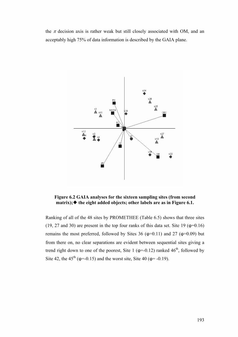
193

the π decision axis is rather weak but still closely associated with OM, and an

acceptably high 75% of data information is described by the GAIA plane.

Figure 6.2 GAIA analyses for the sixteen sampling sites (from second matrix); the eight added objects; other labels are as in Figure 6.1.

Ranking of all of the 48 sites by PROMETHEE (Table 6.5) shows that three sites

(19, 27 and 30) are present in the top four ranks of this data set. Site 19 (φ=0.16)

remains the most preferred, followed by Sites 36 (φ=0.11) and 27 (φ=0.09) but

from there on, no clear separations are evident between sequential sites giving a

trend right down to one of the poorest, Site 1 (φ=-0.12) ranked 46th, followed by

Site 42, the 45th (φ=-0.15) and the worst site, Site 40 (φ= -0.19).

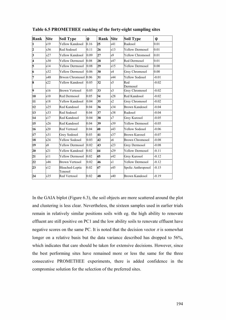
194

Table 6.5 PROMETHEE ranking of the forty-eight sampling sites

Rank Site Soil Type φ Rank Site Soil Type φ 1 s19 Yellow Kandosol 0.16 25 s41 Rudosol 0.01

2 s36 Red Sodosol 0.11 26 s13 Yellow Dermosol 0.01

3 s27 Yellow Kandosol 0.09 27 s9 Yellow Chromosol 0.01

4 s30 Yellow Dermosol 0.08 28 s47 Red Dermosol 0.01 5 s14 Yellow Dermosol 0.08 29 s15 Yellow Dermosol 0.00

6 s32 Yellow Dermosol 0.06 30 s4 Grey Chromosol 0.00

7 s48 Brwon Chromosol 0.06 31 s44 Yellow Sodosol -0.01 8 s22 Yellow Kandosol 0.05 32 s5 Red

Dermosol -0.02

9 s16 Brown Vertosol 0.05 33 s3 Grey Chromosol -0.02

10 s10 Red Dermosol 0.05 34 s28 Red Kandosol -0.02 11 s18 Yellow Kandosol 0.04 35 s2 Grey Chromosol -0.02

12 s25 Red Kandosol 0.04 36 s34 Brown Kandosol -0.04

13 s33 Red Sodosol 0.04 37 s38 Rudosol -0.04 14 s17 Red Kandosol 0.04 38 s7 Grey Kurosol -0.05

15 s26 Red Kandosol 0.04 39 s39 Yellow Dermosol -0.05

16 s20 Red Vertosol 0.04 40 s43 Yellow Sodosol -0.06

17 s31 Grey Sodosol 0.03 41 s37 Brown Kurosol -0.07 18 s24 Yellow Sodosol 0.03 42 s6 Brown Chromosol -0.08 19 s8 Yellow Dermosol 0.02 43 s23 Grey Dermosol -0.08

20 s21 Yellow Kandosol 0.02 44 s29 Yellow Dermosol -0.11

21 s11 Yellow Dermosol 0.02 45 s42 Grey Kurosol -0.12

22 s46 Brown Vertosol 0.02 46 s1 Yellow Dermosol -0.12

23 s12 Bleached-Leptic Tenosol

0.02 47 s45 Spolic Anthroposol -0.15

24 s35 Red Vertosol 0.02 48 s40 Brown Kandosol -0.19

In the GAIA biplot (Figure 6.3), the soil objects are more scattered around the plot

and clustering is less clear. Nevertheless, the sixteen samples used in earlier trials

remain in relatively similar positions soils with eg. the high ability to renovate

effluent are still positive on PC1 and the low ability soils to renovate effluent have

negative scores on the same PC. It is noted that the decision vector π is somewhat

longer on a relative basis but the data variance described has dropped to 56%,

which indicates that care should be taken for extensive decisions. However, since

the best performing sites have remained more or less the same for the three

consecutive PROMETHEE experiments, there is added confidence in the

compromise solution for the selection of the preferred sites.

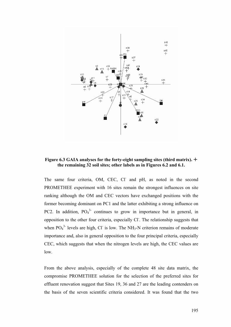
195

Figure 6.3 GAIA analyses for the forty-eight sampling sites (third matrix). the remaining 32 soil sites; other labels as in Figures 6.2 and 6.1.

The same four criteria, OM, CEC, Cl- and pH, as noted in the second

PROMETHEE experiment with 16 sites remain the strongest influences on site

ranking although the OM and CEC vectors have exchanged positions with the

former becoming dominant on PC1 and the latter exhibiting a strong influence on

PC2. In addition, PO43- continues to grow in importance but in general, in

opposition to the other four criteria, especially Cl-. The relationship suggests that

when PO43- levels are high, Cl- is low. The NH3-N criterion remains of moderate

importance and, also in general opposition to the four principal criteria, especially

CEC, which suggests that when the nitrogen levels are high, the CEC values are

low.

From the above analysis, especially of the complete 48 site data matrix, the

compromise PROMETHEE solution for the selection of the preferred sites for

effluent renovation suggest that Sites 19, 36 and 27 are the leading contenders on

the basis of the seven scientific criteria considered. It was found that the two

196

criteria, CEC and OM, conventionally used for the initial appreciation of soil

quality for this purpose, remain critically important for the selection of the best

performing soils. However, the low ability soils tend to be discriminated from the

high ability ones by pH and Cl- levels. In addition, PO43- and to a lesser extent

NH3-N criteria provide further important discrimination of the sites. Thus, the

compromise solution has to be based on the consideration of at least CEC, OM,

pH, Cl- as well as PO43- and NH3-N. Interestingly, EC seems to play a relatively

low role in the site selection.

In soils ranking and the selection of several sites for sewage effluent renovation, it

was necessary to take into account the size of the π decision axis (just moderate

size) and the fact that only 56% of data variance has been described. Some

assistance may be obtained from the results of the first two PROMETHEE and

GAIA experiments. The decision-maker may observe that in the second MCDM

analysis, Sites 10 and 12 were ranked in the top eight samples, but clustered with

the poorer soils in the GAIA plot of the first two PROMETHEE experiments

(negative scores on PC1). Also, the rank order of the 48 sites show that five sites

19, 27, 30, 22, and 16, which were ranked highly in the smaller matrix trials,

appear in the first nine rankings before Site 10 (a poor site, ranking 10).

Conservatively therefore, on the balance of information available there is an

additional six sites (ranking 4-9) prior to Site 10.

The PROMETHEE analysis for the forty-eight sites provided a ranking system for

the sites’ ability to renovate effluent based on the seven physico-chemical

parameters previously investigated. The results obtained were based on the initial

input criteria submitted to PROMETHEE (Table 6.2). These criteria were

obtained from the soil analysis in Chapter 4. The changes in the initial criteria

input could change the ranking outcome. Therefore, it was important to indicate

that both methods (conventional and PROMETHEE) have to be used together for

evaluating the soil ability to renovate effluent, as they complement each other,

which will result in more accurate site evaluations.

197

6.4 Long Term Acceptance Rate (LTAR) The ability of the soil medium to remove pollutants and transmit effluent is one of

soils’ more important characteristics and one which a successful on-site sewage

treatment system is significantly dependent. On-site wastewater treatment relies

on infiltration and percolation of primary effluent through soil to achieve

satisfactory purification prior to recharge to ground water (US EPA, 1978; US

EPA, 1980; Jenssen and Siegrist, 1990). These systems can achieve high

purification efficiencies due to the complex interactions of hydraulic and physico-

chemical processes (Stevik et al., 1999). Due to the extensive contact between

wastewater constituents and the soil matrix, a biofilm (clogging mat) will form on

the soil interaction surface as a result of the deposition of solids and microbial

action as discussed in Section 2.3. In general, there are a number of factors

affecting the formation of the clogging layer such as soil type, wastewater quality

and load, anaerobic conditions, pH and environmental conditions such as

temperature and moisture content (Laak, 1973). These factors should be

considered in understanding soil behaviour under effluent application. The

percolation rate of effluent into soil will change as a result of clogging mat

formation. The percolation rate will reach an almost constant value over time,

which is referred to as the long-term acceptance rate (LTAR) for the soil. The

LTAR values for 12 soils in the soil column experiment (Chapter 5) are necessary

for designing the subsurface trenches to distribute the discharged septic tank

effluent to the subsurface soils. The LTAR values are useful tools to reduce the

risk for future systems failure.

The results obtained from the column experiment discussed in Chapter 5 together

with the outcomes from the field soil sampling and testing (Chapter 4) were used

for determining the LTAR for the selected twelve soil types. The column

experiment for undisturbed soils was an important stage in the research

undertaken. The previous studies by other researchers mostly concentrated on

surface application with disturbed soils and the build up of OM on the soil

surface. The column study provided the advantage to investigate the influence of

the build up of OM on different undisturbed soils . Also, the study considered the

influence of soil mineralogy on effluent percolation within the different soil

horizons.

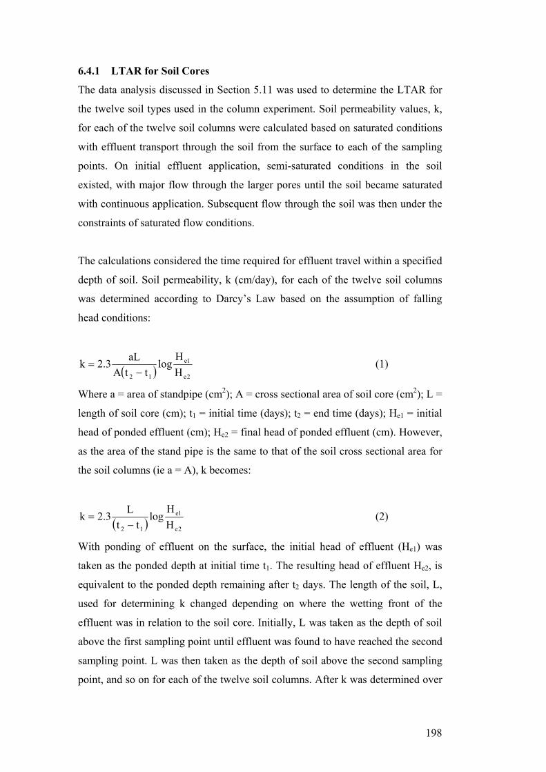
198

6.4.1 LTAR for Soil Cores

The data analysis discussed in Section 5.11 was used to determine the LTAR for

the twelve soil types used in the column experiment. Soil permeability values, k,

for each of the twelve soil columns were calculated based on saturated conditions

with effluent transport through the soil from the surface to each of the sampling

points. On initial effluent application, semi-saturated conditions in the soil

existed, with major flow through the larger pores until the soil became saturated

with continuous application. Subsequent flow through the soil was then under the

constraints of saturated flow conditions.

The calculations considered the time required for effluent travel within a specified

depth of soil. Soil permeability, k (cm/day), for each of the twelve soil columns

was determined according to Darcy’s Law based on the assumption of falling

head conditions:

( ) 2e

1e

12 HH

logttA

aL3.2k−

= (1)

Where a = area of standpipe (cm2); A = cross sectional area of soil core (cm2); L =

length of soil core (cm); t1 = initial time (days); t2 = end time (days); He1 = initial

head of ponded effluent (cm); He2 = final head of ponded effluent (cm). However,

as the area of the stand pipe is the same to that of the soil cross sectional area for

the soil columns (ie a = A), k becomes:

( ) 2e

1e

12 HH

logtt

L3.2k−

= (2)

With ponding of effluent on the surface, the initial head of effluent (He1) was

taken as the ponded depth at initial time t1. The resulting head of effluent He2, is

equivalent to the ponded depth remaining after t2 days. The length of the soil, L,

used for determining k changed depending on where the wetting front of the

effluent was in relation to the soil core. Initially, L was taken as the depth of soil

above the first sampling point until effluent was found to have reached the second

sampling point. L was then taken as the depth of soil above the second sampling

point, and so on for each of the twelve soil columns. After k was determined over

199

the length of effluent application, the LTAR for each of the twelve columns was

determined according to equation given by Laak (1986):

klog2.1k5LTAR −= (3)

where

LTAR= Long Term Acceptance Rate (cm/Day),

k = soil permeability (cm/s).

The flow of effluent through the soil core will depend on the formation of the

clogging layer. Consequently, as the clogging layer develops, the flow of effluent

through the soil will reduce accordingly until the LTAR is reached.

6.4.2 Example for the k Value Calculation

The example given below illustrates the k value calculations. The k values were

calculated based on the soil depth and the time effluent samples were collected

from each sampling point. The k values for Column 1 (Yellow Kurosol) were

calculated as shown below and in the same way the k values were calculated for

the other soil types.

The soil depth for the first effluent sampling point was considered in the

calculation. The distance for the first effluent sampling point was 110mm and for

the second effluent sampling point was 415mm. The calculations are shown in

Table 6.6.

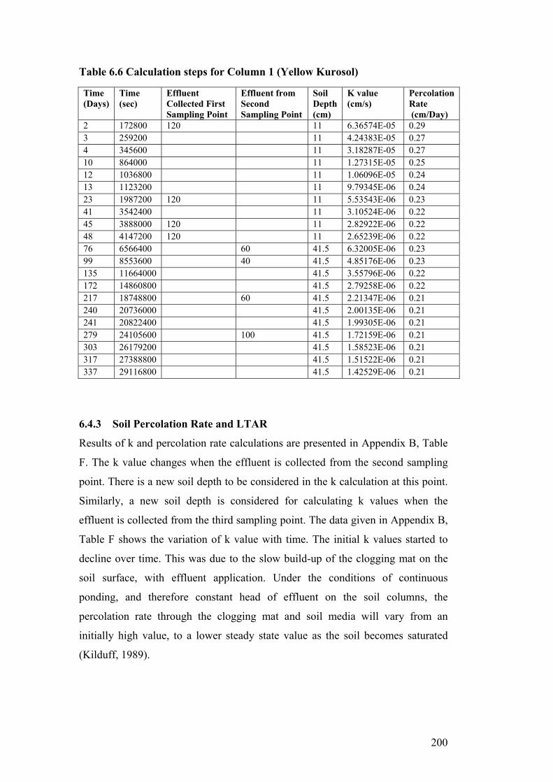
200

Table 6.6 Calculation steps for Column 1 (Yellow Kurosol)

Time (Days)

Time (sec)

Effluent Collected First Sampling Point

Effluent from Second Sampling Point

Soil Depth (cm)

K value (cm/s)

Percolation Rate (cm/Day)

2 172800 120 11 6.36574E-05 0.29 3 259200 11 4.24383E-05 0.27 4 345600 11 3.18287E-05 0.27 10 864000 11 1.27315E-05 0.25 12 1036800 11 1.06096E-05 0.24 13 1123200 11 9.79345E-06 0.24 23 1987200 120 11 5.53543E-06 0.23 41 3542400 11 3.10524E-06 0.22 45 3888000 120 11 2.82922E-06 0.22 48 4147200 120 11 2.65239E-06 0.22 76 6566400 60 41.5 6.32005E-06 0.23 99 8553600 40 41.5 4.85176E-06 0.23 135 11664000 41.5 3.55796E-06 0.22 172 14860800 41.5 2.79258E-06 0.22 217 18748800 60 41.5 2.21347E-06 0.21 240 20736000 41.5 2.00135E-06 0.21 241 20822400 41.5 1.99305E-06 0.21 279 24105600 100 41.5 1.72159E-06 0.21 303 26179200 41.5 1.58523E-06 0.21 317 27388800 41.5 1.51522E-06 0.21 337 29116800 41.5 1.42529E-06 0.21

6.4.3 Soil Percolation Rate and LTAR

Results of k and percolation rate calculations are presented in Appendix B, Table

F. The k value changes when the effluent is collected from the second sampling

point. There is a new soil depth to be considered in the k calculation at this point.

Similarly, a new soil depth is considered for calculating k values when the

effluent is collected from the third sampling point. The data given in Appendix B,

Table F shows the variation of k value with time. The initial k values started to

decline over time. This was due to the slow build-up of the clogging mat on the

soil surface, with effluent application. Under the conditions of continuous

ponding, and therefore constant head of effluent on the soil columns, the

percolation rate through the clogging mat and soil media will vary from an

initially high value, to a lower steady state value as the soil becomes saturated

(Kilduff, 1989).

201

The infiltrative rate through the soil columns retained similar phases to that

highlighted by Allison (1947), Jones and Taylor (1965), Thomas et al. (1966), and

Okubo and Matsumoto (1979) as discussed in Chapter 2. Figures 6.4a to 6.4l

provide charts of percolation rate versus time and the corresponding LTAR value

for the twelve soil columns. All columns had an initial decline in percolation due

to soil pore reduction as a result of suspended solids in the effluent. Following

this, percolation generally increased depending on several factors. The application

of effluent caused the soil cores to become saturated over time, with the removal

of trapped air as the effluent-wetting front moved through the soil. However,

some columns had a more rapid decline in soil percolation as a result of the

column mineralogy and resulting clay content. Clays typically have hydraulic

conductivies in the order of 10-4 to 10-10 depending on the type and amount of clay

present in the soil (Craig, 1997). Consequently, the natural saturated soil

percolation rate (SSPR) of the columns will depend on the soil mineralogy.

Several of the columns (Columns 1, 2, 6, 7, 8, 10, 11 and 12) had an initial decline

in percolation rate that was much lower than the final LTAR value obtained. It is

hypothesised that for these soil types, the final LTAR value is greater than the

SSPR. In other words, the soil’s natural percolation rate is lower than the long

term infiltrative rate obtained after the development of the clogging mat.

An increase in percolation rate was observed in some columns when effluent

reached the respective sampling ports. This is related to an increase in the rate of

escaping trapped air through the sampling port, rather than upwards through the

soil column, thereby allowing faster saturation of the soil to occur. Subsequent

decreases in effluent percolation rate generally occurred as the infiltrative rate

reached LTAR. How rapid this decrease in effluent infiltration occurred was also

dependent on several factors. Infiltration into the soil column was dependent on

the extent to which the clogging mat had already developed. This in turn is

dependant on effluent quality, soil pore size and time. However, as the quality of

effluent was the same for all columns, the rate at which the clogging mat

developed was dependent only on the respective soil pore size.

In general, a sandy soil with larger pore sizes would allow suspended and

dissolved material to penetrate further into the soil matrix, resulting in a thicker

202

active zone and subsequently increasing the time for LTAR to be reached (Healy

and Laak, 1974). This is evident in Column 3 (Figure 6.4c), where an LTAR value

was not reached during the experiment. As such, a slower decline in infiltration

through sandy soil is expected, resulting in high LTAR values as compared to

clayey soils. The rate of infiltration and its respective decline is also dependent on

the hydraulic gradient which is necessary to push the effluent through the

developing clogging layer and into the soil. Consequently, a higher hydraulic

gradient will occur after ponding of effluent on the soil surface with each

application of effluent. This temporary increase in the hydraulic capacity as a

result of newly applied effluent will cause minor increases in infiltration, which

will eventually return to an equilibrium condition. This phenomenon was

observed throughout the experiment. The mineralogy for the twelve soil columns

is reported in Table 6.7.

6.4.4 Behaviour of Individual Columns

The behaviour the individual soil columns are discussed based on the data

provided in Figure 6.4 and Appendix B, Table F. Due to the relative similarity

between columns that retained similar soil types and conditions, the columns are

discussed based on their respective soil types.

203

Table 6.7 Twelve soil columns mineralogy and data

Soil Mineralogy (%) Major Soil Group

Sub-Order

Column No.

Sample Depth (mm) Quartz Kaolinite Illite Smectite Amorphous

Soil Texture

110 60 21 0 0 19 Sandy Loam 415 30 42 0 3 25 Clay Loam

Yellow 1

715 40 21 0 8 31 Clay Loam 130 61 23 5 0 11 Sandy Clay

Loam 430 75 14 4 0 7 Sandy Clay

Loam

Kurosol

Brown 6

730 64 24 4 0 8 Sandy Clay Loam

150 14 57 27 0 2 Clay 450 9 67 21 0 3 Clay

Hydrosol Red 2

750 22 66 0 10 2 Clay 50 94 3 0 0 3 Sand 400 96 0 0 0 4 Sand

Podosol Semiaquic 3

700 90 3 0 0 7 Sand 80 69 16 0 0 15 Sandy Loam 440 68 28 0 1 3 Sandy Clay

Loam

Sodosol Black 4

740 40 20 0 6 34 Loam 120 82 12 0 0 6 Loamy Sand 480 76 20 0 0 4 Sandy Loam

Vertosol Brown 7

780 56 43 0 0 1 Sandy Clay 110 75 2 0 0 23 Loamy Sand 470 77 4 4 0 15 Sandy Loam

Red 5

770 51 39 0 0 10 Sandy Clay 80 87 11 1 0 1 Loamy Sand 440 75 14 4 0 7 Sandy Loam

Brown 8


50 91 3 0 0 6 Sand 410 94 3 0 0 3 Sandy Loam

Dermosol

Yellow 9

710 72 15 0 0 13 Sandy Loam 20 79 19 0 0 2 Sandy Loam 380 66 24 0 0 10 Sandy Clay

Loam

Yellow 10


60 91 4 0 0 5 Sand 420 71 5 0 0 24 Sandy Loam

Chromosol

Grey 11

720 40 48 9 0 3 Clay 80 88 5 5 0 2 Loamy Sand 440 57 14 27 0 2 Sandy Clay

Kandosol Red 12

740 57 19 21 0 3 Sandy Clay

204

Kurosol Soil – Columns 1 and 6

Figures 6.4a and 6.4f provide curves of percolation rate vs time for the two

Kurosol soil columns, Column 1 and Column 6 respectively. Similar results were

observed in both columns, with steady state conditions as a result of the

development of the clogging mat occurring towards the end of the experiment

with LTAR values between 0.205 to 0.211 cm/day. For both columns, ponding

occurred within the first three days of effluent application, mostly as a result of

the naturally low soil permeability. Additionally, slight increases in the

percolation rate after 76 days, and also at 176 days for Column 6 were observed.

These increases occurred when effluent reached the second sampling point (and

subsequently the third sampling point for Column 6). This is postulated to be a

result of trapped air escaping through the sampling points as the soil became

saturated. Due to the effluent reaching the first sampling point at approximately

the same time, indicates that the soil permeability and subsequent percolation

rates are very similar. Slight differences were, however, observed at different

stages of the experiment, and this is hypothesised to be a result of the variations in

the soil’s texture and mineralogy.

The Yellow Kurosol in Column 1 changes from a sandy loam in the top 110mm to

a clay loam in the lower 605mm of the soil, as shown in Table 6.7. This is related

to an increase in clay content through the soil profile with a majority of the clay

being kaolinite, with a high percentage in the middle of the column. Also, small

amounts of smectite (shrink/swell clay) were found, also increasing down through

the soil in the lower part of the soil column. Due to the shrink swell properties of

this clay, an impermeable barrier will form when the smectite saturates and swells

reducing effluent flow through the soil. Additionally, the large amount of

kaolinite clay in the middle of the column caused a rapid decline in the

percolation rate until saturation occurred. Consequently, this clay governed the

initial rate of percolation until clogging of the soil pores occurred and the resultant

LTAR values of 0.205 cm/day were reached. This occurred after 337 days of

effluent application.

The Brown Kurosol soil in Column 6 had similar amounts of clay dispersed

throughout the length of the column. However, no smectite clay was evident.

205

Small percentages of illite clay were however present. This corresponds with the

previous observation that as a result of the shrink/swell properties of the soil in

Column 1, effluent flow through the smectite was minimal. Hence, effluent was

able to reach the third sample point in Column 6, but not Column 1. The other

main difference was related to the amount of sand (quartz) found in the columns.

Column 1 had reducing percentages of quartz, and corresponding clay increases

down the column, whereas Column 6 had fairly constant amount of quartz

throughout the column.

The resulting LTAR values obtained for the Kurosol soils indicate very similar

values (0.205-0.211 cm/day), occurring in approximately the same amount of time

(325 to 337 days). However, due to the restrictive layer developed in Column 1,

its suitability for effluent disposal will be limited.

Hydrosol – Column 2

The Hydrosol soil in Column 2 reached an LTAR value of 0.204cm/day after 130

days of effluent application as shown in Figure 6.4b, which is less than half the

time as for the Kurosol soil. As highlighted in Table 6.7, the soil is described as a

clay soil, as a result of the large amount of clay relative to the amount of quartz in

the soil. Consequently, this affected the initial SSPR, and the rate of development

of the clogging layer. Due to a higher percentage of clay in the top 150mm of soil,

smaller pore spaces between the soils would be expected. Hence, a larger amount

of solid material would be filtered out of the effluent as it passed through the soil.

This would essentially increase the rate of development of the clogging layer,

although it may not be as thick. Additionally, due to the larger percentage of clay,

flow through the soil was restricted causing ponding to occur after only two days

of effluent application.

A similar increase in percolation rate occurred when effluent reached the second

and third sampling points after 76 and 316 days respectively. Again, this is

attributed to the release of trapped air as the soil became saturated. It was not

possible to draw clear conclusions in regards to further soil behaviour after the

increase in percolation rate after 316 days as the experiment was terminated at this

206

point in time. However it is hypothesised that the percolation rate would once

again decline to the accepted LTAR value of 0.204 cm/day after a period of time.

Podosol Soil – Column 3

The percolation rate for the Podosol soil in Column 3 did not reach the LTAR

throughout the course of the experiment as shown in Figure 6.4c. This soil’s

mineralogy indicated that 97% was quartz (sand) and the rest consisted of

amorphous material, a mixture of organic matter and various mineral precipitates.

The first samples collected were from the fourth sampling point located at the

bottom of the column after about five minutes of effluent application. The

clogging mat did not develop over the course of effluent application and effluent

did not pond on the soil infiltrative surface.

This soil has a high k value due to the soil mineralogy which mostly consisted

quartz (Table 6.7). Therefore, effluent percolated quickly through the soil profile,

not allowing adequate time for microbial decomposition and entrapment of solid

matter to occur and form the clogging mat as for other soils. Effluent samples

were collected from the third sampling point after closing the fourth sampling

point and the same procedure was adopted for the second and upper sampling

points. Examining Figure 6.4c, there is an indication of a reduction in the

percolation rate between the four sampling points which shows that the lowest

percolation rate was achieved after 60 days of effluent application. This is due to

the increase in organic matter content within the soil profile as a result of effluent

application and the formation of algae on the soil surface and the sides of the

column. Consequently, as no clogging mat formed throughout the experiment, it

was surmised that the declining percolation towards the end of effluent

application was, as a result of clogging due to the growth of algae. As a result of

this, it was found Column 3 required a much longer time to reach the LTAR than

the period that was allowed for this experiment. However, the current trend shown

in Figure 6.4c suggests that steady state flow conditions were beginning to

develop. The effluent application for Column 3 was stopped shortly after about 60

days.

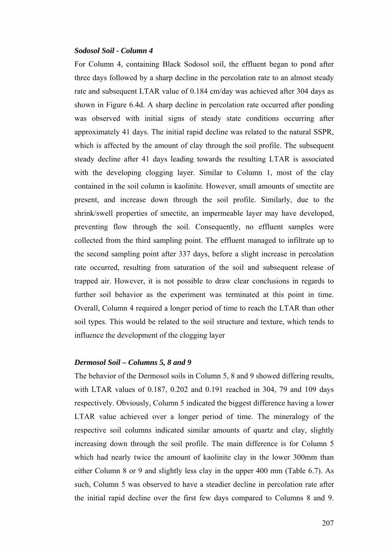
207

Sodosol Soil - Column 4

For Column 4, containing Black Sodosol soil, the effluent began to pond after

three days followed by a sharp decline in the percolation rate to an almost steady

rate and subsequent LTAR value of 0.184 cm/day was achieved after 304 days as

shown in Figure 6.4d. A sharp decline in percolation rate occurred after ponding

was observed with initial signs of steady state conditions occurring after

approximately 41 days. The initial rapid decline was related to the natural SSPR,

which is affected by the amount of clay through the soil profile. The subsequent

steady decline after 41 days leading towards the resulting LTAR is associated

with the developing clogging layer. Similar to Column 1, most of the clay

contained in the soil column is kaolinite. However, small amounts of smectite are

present, and increase down through the soil profile. Similarly, due to the

shrink/swell properties of smectite, an impermeable layer may have developed,

preventing flow through the soil. Consequently, no effluent samples were

collected from the third sampling point. The effluent managed to infiltrate up to

the second sampling point after 337 days, before a slight increase in percolation

rate occurred, resulting from saturation of the soil and subsequent release of

trapped air. However, it is not possible to draw clear conclusions in regards to

further soil behavior as the experiment was terminated at this point in time.

Overall, Column 4 required a longer period of time to reach the LTAR than other

soil types. This would be related to the soil structure and texture, which tends to

influence the development of the clogging layer

Dermosol Soil – Columns 5, 8 and 9

The behavior of the Dermosol soils in Column 5, 8 and 9 showed differing results,

with LTAR values of 0.187, 0.202 and 0.191 reached in 304, 79 and 109 days

respectively. Obviously, Column 5 indicated the biggest difference having a lower

LTAR value achieved over a longer period of time. The mineralogy of the

respective soil columns indicated similar amounts of quartz and clay, slightly

increasing down through the soil profile. The main difference is for Column 5

which had nearly twice the amount of kaolinite clay in the lower 300mm than

either Column 8 or 9 and slightly less clay in the upper 400 mm (Table 6.7). As

such, Column 5 was observed to have a steadier decline in percolation rate after

the initial rapid decline over the first few days compared to Columns 8 and 9.

208

Consequently, a difference in the development of LTAR values is noticeable in

Figures 6.4e, 6.4h and 6.4i respectively.

Each column had an initial rapid decline in percolation rate, with corresponding

pond time of two days for Column 5 and three days for Columns 8 and 9. The

percolation rate declined to a steady rate for Column 5 until an LTAR of 0.187

cm/day was achieved after 304 days. Conversely, Columns 8 and 9 both had a

more rapid decline in SSPR until effluent reached the second sampling point after

73 and 109 days respectively. A slight increase was observed, followed by a

steady decline to reach LTAR values of 0.202 and 0.191 cm/day for Columns 8

and 9. Similar to Columns 1 and 6, the main reasons for the difference between

the Dermosol soils would mostly be related to the soil suborders and soil

mineralogy. Longer times would be required for the development of the clogging

mat for soil that had higher amounts of sand as deeper penetration of OM and

solid material into the soil would be possible as for Column 5 in the top 110 mm.

Hence, more time will be required to achieve sufficient reduction in pore size and

subsequent clogging of the soil than soils with higher clay contents.

Vertosol Soil – Column 7

The Vertosol soil in Column 7 ranges from a loamy sand at the top 120 mm to a

sandy clay in the lower 300 mm. Particular importance is the large percentage of

clay in the lower 300 mm (43% kaolinite – see Table 6.7) which will have an

appreciable influence on the flow of effluent through the soil. Hence, a decreasing

permeability as a result of the soil’s increasing clay content prior to clogging

development was expected, and is evident in the curves shown in Figure 6.4g. As

a result of this decreasing permeability, ponding occurred after three days of

effluent application. The initial rapid decline in percolation rate, which only

tended towards steady state conditions after 41 days, is due to the increase in clay

content through the soil profile. As depicted in Figure 6.4g, the natural SSPR was

never reached prior to an LTAR of 0.216 cm/day being achieved after 338 days.

This indicates that the SSPR is in fact less than the developed LTAR values

governed by flow through the clogging layer. The results from Column 7 suggest

that Vertosol soils may not be suitable for effluent dispersal. Additionally, flow

209

through this particular soil would be governed by the SSPR and not the LTAR

value.

Chromosol Soils – Columns 10 and 11

The resulting curves for Columns 10 and 11 shown in Figure 6.4j and 6.4k

indicate distinct differences in the LTAR values and the time to reach steady state

conditions. Column 10 showed similar processes to that for Column 7 (Vertosol

soil), with a rapid decrease in SSPR after only 23 days, by which time the effluent

had reached the second sampling point (passing through 20 mm of soil) and an

increase in percolation occurred due to the release of trapped air through the

second sampling point. Chromosol soils are defined by their abrupt increase in

clay content (> 20% difference between soil horizons), (Isbell 1996), and as

shown in Table 6.7. The resulting decline in percolation rate after this headed

towards steady state conditions, but did not reach an appropriate LTAR value as a

result of clogging mat development after 338 days. As found in Column 7, the

SSPR for Column 10 was much lower than the predicted LTAR value of 0.200

cm/day, and the SSPR for the Chromosol soil in Column 10 would govern the

flow through the soil.

On the other hand, Column 11, which also shows a significant increase in clay

content (Table 6.7), although having an initial rapid decline, seemed to head

towards steady state conditions and LTAR before effluent reached the second

sampling point. At the second sampling point there appears to be a steady decline

towards LTAR. However, it did not reach the accepted LTAR of 0.183 cm/day

before the end of the experiment period. An increase in the percolation rate after

247 days was observed and was found to be related to an accumulation of fine

particles in the effluent collection tube inside the soil column. Once this was

cleared, a higher percolation rate was recorded. Similar to the Dermosol soils, the

time required for the development of the clogging layer and subsequent LTAR is

dependant on the soil structure and texture. Column 10 had less quartz in the

upper 300 mm of soil than Column 11, and therefore, more rapid clogging would

occur due to the finer soil pore size.

210

Kandosol Soil – Column 12.

The Red Kandosol soil in Column 12 almost reached the LTAR of 0.212 cm/day

after 338 days of effluent application, even though this value was originally

reached after 42 days at the first sampling point. Similar to Kurosol soil (Columns

1 and 6) and Dermosol soils (Columns 8 and 9), this was caused by a rapid

reduction in percolation rate as the soil became saturated and neared its SSPR.

However, the true LTAR value produced by clogging of the infiltrative surface

only began to occur towards the end of effluent application, at 338 days.

Consequently, the resulting SSPR would be less than the actual LTAR value,

indicating that the percolation rate for the soil is most likely governed by the

SSPR rather than the LTAR value. As for the other columns, the main reason for

the rapid decline towards SSPR is a result of the large amount of clay in the soil

as highlighted in Table 6.7, which resulted in rapidly declining soil permeability

and therefore percolation rate as the soil became saturated. The slight increase in

percolation rate during the experiment occurred when effluent reached the

respective sampling points, forcing out air through them as the soil became

saturated.

211

Figure a

LTAR

0.190

0.210

0.230

0.250

0.270

0.290

0.310

0 100 200 300 400

Days

Pero

clat

ion

Rat

e (c

m/d

)

Percolation Rate 1stSampling Point

Percoalation Rate 2ndSampling Point

LTARPonding observedday 3

Figure b

LTAR

0.190

0.210

0.230

0.250

0.270

0.290

0.310

0 100 200 300 400

Days

Pero

clat

ion

Rat

e (c

m/d

)



Percolation Rate 3rdSampling Point

LTAR

Ponding observed day 2

Figure c

0.15

0.17

0.19

0.21

0.23

0.25

0.27

0.29

0.31

0 20 40 60 80

Days

Pero

clat

ion

Rat

e (c

m/d

)

Percolation Rate 1st SamplingPoint

Percoalation Rate 2nd SamplingPoint

Percolation Rate 3rd SamplingPoint

Percolation Rate 4th SamplingPoint

Figure d

LTAR0.170

0.190

0.210

0.230

0.250

0.270

0.290

0.310

0 100 200 300 400

Days

Pero

clat

ion

Rat

e (c

m/d

)



LTARPonding observed day 3

Figure 6.4 LTAR for columns 1, 2, 3 and 4

212

Figure e

LTAR

0.150

0.170

0.190

0.210

0.230

0.250

0.270

0.290

0.310

0 100 200 300 400

Days

Pero

clat

ion

Rat

e (c

m/d

)



LTAR


Figure f

LTAR

0.190

0.210

0.230

0.250

0.270

0.290

0.310

0 100 200 300 400

Days

Pero

clat

ion

Rat

e (c

m/d

)




LTAR


Figure g

LTAR

0.190

0.210

0.230

0.250

0.270

0.290

0.310

0 100 200 300 400

Days

Pero

clat

ion

Rat

e (c

m/d

)



LTAR



Figure h

LTAR0.190

0.210

0.230

0.250

0.270

0.290

0.310

0 100 200 300 400

Days

Pero

clat

ion

Rat

e (c

m/d

)




LTAR


Figure 6.4 LTAR for columns 5, 6,7 and 8

213

Figure 6.4 LTAR for columns 9, 10, 11 and 12

214

6.4.5 Summary of Observations

The long-term acceptance rate for the investigated soils was achieved for most

columns except for Column 3, although the time taken to reach the respective

LTAR value varied as shown in Table 6.8. The LTAR was achieved for the

Columns 1, 2 and 8 for the second sampling point at the various soil depths as

discussed. Column 7 achieved the long-term acceptance rate for the third

sampling point at a soil depth of 780 mm and the other columns required a longer

period of time to achieve LTAR than what was allowed during the experimental

period. As shown in Table 6.8, the long-term acceptance rates for eleven of the

twelve investigated soil types fall within a relatively narrow band. However

different time periods were required for the LTAR values to be achieved. This can

be attributed to factors such as soil mineralogy, soil depth and soil structure.

Table 6.8 LTAR for the twelve columns at the first sampling point.

Column Number

Soil Type LTAR cm/Day

Time to Achieve LTAR (Days)

1 Yellow Kurosol 0.205 65 2 Hydrosol 0.204 130 3 Podosol Not Reached Require more time 4 Black Sodosol 0.184 304 5 Red Dermosol 0.187 304 6 Brown Kurosol 0.211 75 7 Brown Vertosol 0.216 41 8 Brown Dermosol 0.202 79 9 Yellow Dermosol 0.191 109 10 Yellow Chromosol 0.200 23 11 Grey Chromosol 0.183 247 12 Red Kandosol 0.212 42

215

6.5 Sites Evaluation Validation The preliminary soil evaluation based mostly on the CEC in the investigated 48

sites (as in Section 6.2) in conjunction with the analytical methods (as in Section

6.3) were validated from the analysis and outcomes from the experimental soil

columns.

To facilitate a multi-variate approach for soil evaluation, well regarded MCDM

methods, PROMETHEE and GAIA, were applied for analysis of a sequence of

three matrices, dimensionally increased from 8x7 to 48x7, and the modelling of

the matrices and the interpretation of results were discussed in detail. From these

analyses, PROMETHEE net outranking flows,ϕ, showed that two Sites 19 and 27

were always among the top three ranks of the three matrices investigated. The

input criteria in the analysis for CEC level and OM were always in agreement

with preliminary analysis, are important for the soil evaluation, but other physico-

chemical criteria should be considered. This was especially apparent with the

analysis of the largest matrix, which undoubtedly represents the common real

world scenario, where more rather than less sites would be desirable to be tested

and analysed together. In addition, it was found that the pH and Cl- attributes were

related to the discrimination of the weaker performing sites from the better ones,

and the PO43- and the NH3-N criteria were in general in opposition to CEC, OM,

pH and Cl- but were much less effective as discriminators (shorter loadings

vectors).

The column experiment study was a useful stage in the research undertaken. The

study assisted in understanding the actual soil behaviour under effluent

application. The outcomes of the column study helped to refine the conclusions

derived from soil sampling based on CEC as discussed in Section 6.2. It was

concluded that 25% of the twelve investigated soils have a high ability for effluent

treatment. In addition, the column experimental study indicated that 50% of the

twelve soils have a moderate ability to treat effluent, which requires special

design consideration before discharging effluent. Finally, the study indicated that

25% of the twelve investigated soils have a low ability to treat effluent.

216

There are some common outcomes among the twelve investigated soil cores such

as the following.

• The soils are acidic.

• Effluent application raised the soil pH to become less acidic.

• Effluent application increased the dissolved organic matter content within

the soil profile.

• Most of the soils have a higher ability to renovate phosphorus than nitrogen.

• The preferable CEC range was between 15 and 40 meq/100g for the soils to

provide the required effluent treatment.

• Effluent transmission has a large impact on the soil’s ability to treat effluent.

• Most of the individual exchangeable cations in the soil columns are leached

to the subsurface layers.

• Most of the soils are dominated by Mg2+ cations.

• In most cases, the soil Ca:Mg ratio decreased with the increase of ESP and

vice versa.

• The wetting points for each soil is dependent on the soil mineralogy.

From the results of the undisturbed soil columns studies, several major factors

were found to influence the flow through the soil, and the development of the

clogging layer. Firstly, all soil columns, except Column 3, retained LTAR values

in the range of 0.18 to 0.22 cm/day. However, the required time for the

percolation rate of effluent to reach these observed results varied markedly, from

41 days to 304 days. This is caused by varying factors, including effluent quality

and loading rates, and soil properties such as structure, texture and mineralogy.

The results of the study confirmed that the soil mineralogy and subsequent texture

has an influence over the development of the clogging layer. A sandy soil will

allow high levels of solid and organic material to penetrate further into the soil

matrix, thereby causing thicker clogging layer to develop over a longer time

period. Conversely, in clayey soils, more rapid clogging of soil pores will occur as

a result of the smaller pore sizes causing enhanced entrapment of solid material.

The thickness of the clogging layer will also be less.

217

Another important outcome obtained through this study on undisturbed soil cores

is that in some cases, flow through the soil may be governed more by the natural

saturated soil percolation rate (SSPR), rather than by the LTAR obtained through

the development of the clogging layer. This was noticeable in several columns

with a rapid decline in percolation rate from the beginning of effluent application,

and may have continued to the natural SSPR if clogging did not affect the

subsequent flow.

The defined LTAR values are important parameters in the design of on-site

subsurface sewage effluent disposal systems. These data would help to design

appropriate disposal area based on the soil conditions. Using realistic LTAR

values in design will help to reduce the risk of failure of these systems in the

future.

The combined outcomes from the soil evaluation in the three stages: column

experiments, preliminary evaluation and the chemometrics method are

summerised in Table 6.9. The analysis shows that five soil types (Hydrosol,

Podosol, Brown Vertosol, Grey Chromosol) have been matched completely in

three evaluation stages. The outcomes indicate that nine soil types (Yellow

Kurosol, Hydrosol, Podosol, Red Dermosol, Brown Vertosol, Brown Dermosol,

Yellow Chromosol, Grey Chromosol and Red Kandosol) have matched in the

preliminary evaluation and with the column experiments. Also, the results indicate

that seven soil types (Hydrosol, Podosol, Brown Kurosol, Brown Vertosol,

Yellow Dermosol, Grey Chromosol and Red Kandosol) have matched in the

statistical evaluation and with the soil column experiment evaluation. In

conclusion, the three evaluation stages provided valuable information about the

soil performance. The soil performance under effluent application in the column

experiment is considered the baseline for soils evaluation because it reflects the

actual soil behaviour. The preliminary evaluation based on the soil physico-

chemical characteristics comes as a second choice after the column experiment.

The analytical method is used in conjunction with preliminary evaluation to fill

the gaps in the soil performance understanding.

218

There are different reasons for the variation in the evaluation between the column

experiments and the preliminary methods. Firstly, the evaluation using the

preliminary method is mostly based on the soil physico-chemical data, but the

column evaluation is based on the soil physico-chemical, effluent data and the

observations made during the experiment such as shrink/swell behaviour and

effluent ponding. Secondly, the physico-chemical data used for preliminary

evaluation mostly were CEC, pH and organic matter content. Thirdly, the column

experiment was able to consider the effluent transmission through the soil and this

information was not available for the preliminary evaluation. Finally, the soil

columns present actual soils’ performance, but the preliminary evaluation was

based on information available in published literature and information obtained in

the field.

The variation between the column experiments and the chemometrics method

adopted is related to different factors such as:

1. Human factor; the data output is controlled by the initial input criteria used

which is mostly based on subjective judgment.

2. Soil physical factors; the evaluation does not consider the transmission of

effluent through the soil.

3. Preliminary analysis; the data evaluation is mostly based on the data analysis

conducted in the preliminary stage. Any artifacts in the preliminary evaluation

will be carried over to the analytical methods.

4. Data; the large amount of data increased the margin of error between the

evaluated sites due to soil heterogeneity and composition.

219

Table 6.9 Soils evaluation from the three stages

Soil type Soil Column (Affluent

Sites Evaluation (Preliminary)

Sites Evaluation (Analytical)

Comments

Yellow Kurosol Moderate ability Moderate ability Low Under estimated by the analytical method

Hydrosol High ability High ability High ability The evaluation matches 100%

Podosol Low ability Low ability Low ability The evaluation matches 100%

Black Sodosol High ability Moderate ability Moderate ability Under estimated by the preliminary and analytical mehods.

Red Dermosol Low ability Low treatment Moderate ability Over estimated by the analytical method

Brown Kurosol Low ability Moderate ability Low ability Over estimated by the theoretical site evaluation due to moderate exchange capacity

Brown Vertosol Moderate ability Moderate ability Moderate ability The evaluation matches 100%

Brown Dermosol Moderate ability Moderate ability Low ability Under estimated by the analytical

Yellow Dermosol Moderate ability Low ability Moderate ability Under estimated by the theoretical site evaluation due to the low CEC found by the

Yellow Chromosol Moderate ability Moderate ability High ability Over estimated by the analytical method

Grey Chromosol Moderate ability Moderate ability Moderate ability The evaluation matches 100%

Red Kandosol High ability High ability High ability The evaluation matches 100%

220

Chapter 7 Conclusions and Recommendations 7.1 Site Evaluation Based on Soils’ Physico-chemical

Characteristics Forty-eight sites were investigated for their effluent application suitability. Nine

major soil orders were recorded within the forty-eight investigated sites. The sites

were evaluated based on the soils’ physico-chemical characteristics.

The soil evaluation was mostly based on the soils’ CEC, OM and pH. The soil

CEC is an important property for nutrient retention and supply. The major

outcomes for the site evaluation based on the soils’ physico-chemical

characteristics are:

• All the investigated sites have acidic soils in the range between 5 and 6.5

pH.

• 33% of the investigated sites were considered to have a low ability to treat

the discharged effluent. The outcomes were based on the soil physico-

chemical characteristics.

• 42% of the investigated sites were considered to have a moderate ability to

treat effluent.

• 25% of the investigated sites were considered to have a high ability to treat

effluent.

The limited physico-chemical factors used for evaluating the soil ability to treat

effluent indicated that there was a need for extra analysis to include all the soils’

physico-chemical factors in the evaluation. This extra analysis assisted in

developing a greater in-depth understanding of the soils’ ability to treat effluent.

7.2 Site Evaluations Using Multivariate Analysis The investigated 48 sites were evaluated for their ability to treat effluent using a

multivariate approach to include all the physico-chemical parameters.

PROMETHEE and GAIA were applied for the analysis. The analysis using

PROMETHEE and GAIA indicated the following:

• The most suitable soil was the Kandosol order.

221

• The weakest soil was the Podosol order.

• The GAIA analysis was in agreement with the previous analysis regarding

the OM, CEC and pH.

The multivariate methods used for evaluating the investigated sites’ ability to treat

effluent were based on the input of the initial preference function values. Also, the

GAIA method used for the site evaluation assisted in understanding the

interaction between different physico-chemical parameters.

7.3 Soil Column Study The column experiment study was an important stage of the research. This work

assisted in understanding the actual soil behaviour under effluent application and

for further refining and validating the outcomes derived from the evaluation of

soil physico-chemical characteristics. The results obtained indicated that:

• 25% of the investigated soils have high ability for effluent treatment. This

matches totally with the evaluation based on the CEC, OM and pH.

• 50% of the investigated soils have moderate ability to treat effluent. The

earlier evaluation is matched by 85% with the column study.

• The study indicated that 25% of the soils have low ability to treat effluent.

This evaluation matches by 75% with the previous evaluation.

The original soil cores collected were acidic with pH less than 6.0. Effluent

application raised the pH value to become less acidic. In addition, the effluent

application increased the dissolved OM within the soil profile. The investigation

showed that most of the soils have a higher ability to renovate phosphorus than

nitrogen.

The soil investigation indicated that the favourable CEC range was between 15

and 40 meq/100g for the soils to provide the required effluent treatment. In

addition to that, effluent transmitted within the soil has a large impact on the soil’s

ability to treat effluent. The investigations found that most of the individual

cations are leached to the subsurface layers because of effluent application and the

cations are usually dominated by a stronger cation. Also, the study reported that

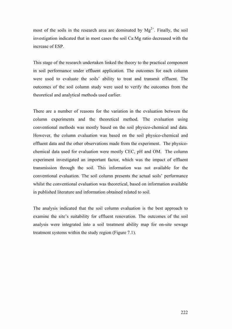
222

most of the soils in the research area are dominated by Mg2+. Finally, the soil

investigation indicated that in most cases the soil Ca:Mg ratio decreased with the

increase of ESP.

This stage of the research undertaken linked the theory to the practical component

in soil performance under effluent application. The outcomes for each column

were used to evaluate the soils’ ability to treat and transmit effluent. The

outcomes of the soil column study were used to verify the outcomes from the

theoretical and analytical methods used earlier.

There are a number of reasons for the variation in the evaluation between the

column experiments and the theoretical method. The evaluation using

conventional methods was mostly based on the soil physico-chemical and data.

However, the column evaluation was based on the soil physico-chemical and

effluent data and the other observations made from the experiment. The physico-

chemical data used for evaluation were mostly CEC, pH and OM. The column

experiment investigated an important factor, which was the impact of effluent

transmission through the soil. This information was not available for the

conventional evaluation. The soil column presents the actual soils’ performance

whilst the conventional evaluation was theoretical, based on information available

in published literature and information obtained related to soil.

The analysis indicated that the soil column evaluation is the best approach to

examine the site’s suitability for effluent renovation. The outcomes of the soil

analysis were integrated into a soil treatment ability map for on-site sewage

treatment systems within the study region (Figure 7.1).

223

Kilometres

Figure 7.1 Soil treatment ability map for on-site sewage treatment

224

7.4 Long-term Acceptance Rate From the results of the undisturbed soil columns study, several factors were found

to influence the flow through the soil, and the development of the clogging layer.

Firstly, all soil columns, except Column 3, attained LTAR values in the range of

0.18 to 0.22 cm/day. However, the required time for the percolation rate of

effluent to reach these observed results varied markedly, from 41 days to 304

days. This is caused by varying factors, including effluent quality and loading

rates, and soil properties such as structure, texture and mineralogy. The results of

the study confirmed that the soil mineralogy and the resulting texture have an

influence on the development of the clogging layer. A sandy soil will allow high

levels of solids and organic material to penetrate further into the soil matrix,

thereby causing a thicker clogging layer to develop over a longer time period.

Conversely, in clayey soils, more rapid clogging of soil pores will occur as a

result of the smaller pore sizes causing enhanced entrapment of solid material.

The thickness of the clogging layer will also be less.

Another important outcome derived through this study was that in some cases,

flow through the soil may be governed more by the natural saturated soil

percolation rate, rather than by the LTAR obtained through the development of

the clogging layer. This was noted in several columns with a rapid decline in

percolation rate from the beginning of effluent application, and may have

continued to the natural SSPR if clogging did not affect the flow.

The defined LTAR values are important parameters in the design of on-site

subsurface sewage effluent disposal systems. These would help to design

appropriate effluent disposal areas based on the soil conditions. Using realistic

LTAR values in design will help to reduce the risk of failure of these systems in

the future.

The long-term acceptance rate was determined for the twelve investigated soils in

the column experiments. The LTAR was determined based on the effluent

transport reduction within different soil depths. The LTAR recorded in this study

reflected the actual soil capacity to transmit the percolating effluent.

225

7.5 Recommendations Further studies are needed to develop better fundamental understanding of the

soils’ ability to treat and transmit sewage effluent. Therefore, it is recommended

that the following studies be undertaken as detailed below.

1. The current study covered twelve soil types and further physico-chemical

analysis is required for the other common soils in the Southeast

Queensland region to develop a complete understanding of the soil data

for the whole region.

2. The study undertaken considered only soil and the effluent characteristics

in the evaluation. However further studies are required to include human

factors or management measures in the evaluation undertaken.

3. The soil columns experiment was conducted for twelve months. However

some soils require a longer period of time to be able to determine the

LTAR. Hence, experiments with longer time spans are recommended.

4. The column study investigated the soils in a vertical dimension. There can

be vertical effluent flow through soil. It is important to understand lateral

flow and the influence of evapotranspiration on the soils’ ability to treat

effluent.

226

Chapter 8 References

Ahern, C. R., R. J. Shaw and V. J. Eldershaw. 1988. Predicated deep drainage loss

of Burdekin soils. Queensland Department of Primary Industries, Bulletin

QB9002.

Alhajjar, B. J., J. M. Harkin and G. Chesters. 1989. Detergent formula and

characteristics of wastewater in septic tanks. Journal of Water Pollution Control

Federation,61(5):605-613.

Allen, B. L. and B. F. Hajek. 1989. Mineral occurrence in soil environments. In:

Minerals in Soil Environments, Dixon, J. B. and S. B. Weed, (Ed). Madison, WI:

SSSA Book Series, 199-278.

Allison, L. E. 1947. Effect of microorganisms on permeability of soil under

prolonged submergence. United States Department of Agriculture. Soil Science,

63:. 439-450.

Al-Shemmeri, T., B. Al-Kloub and A. Pearman. 1997. Model choice in multi-

criteria decision aid. European Journal of Operational Research, 97: 550-560.

American Public Health Association. 1989. Standard Methods for the

Examination of Water and Wastewater - 18th ed. Washington, DC, American

Public Health Association, American Water Works Association and Water

Environment Federation.

Anderson, D. L, J. M. Rice, M. L. Voorhees, R. A. Kirkner, and K. M. Sherman.

1988. Groundwater modeling with uncertainty analysis to assess the

contamination potential from onsite sewage disposal systems in florida. In On-Site

Wastewater Treatment. Fifth National Symposium on Individual and Small

Community Sewage Systems Proceeding. Chicago, IL, 264-273. American Society

of Agricultural Engineering, St. Joseph, MI.

227

Anderson, D. L., M. B. Tyl, R. J. Otis, T. G. Mayer and K. M. Sherman. 1998.

Onsite wastewater nutrient reduction systems (OWNRS) for nutrients sensitive

environments. In On-site Wastewater Treatment: Proceedings of the Eighth

National Symposium on Individual and Small Community Sewage Systems, ed. D.

M. Sievers. American Society of Agricultural Engineering, St. Joseph, MI.

Anikwe, M. A. N. 2000. Amelioration of a heavy clayloam soil with rice husk

dust and its effect on soil physical properties and maize yield. Bioresources

Technology, 74: 169-173.

AS/NZS 1547:2000. 2000. Onsite domestic –wastewater management,

Australia/New Zealand Standard. Standards Australia/New Zealand.

Bailey, S. W. 1984. Micas. Reviews in Mineralogy, Washington DC.

Mineralogical Society of America, 13: 1-584.

Bailey, S. W. 1988. Reviews in Mineralogy. Hydrous Phyllosilicates (exclusive of

micas), Washington DC. Mineralogical Society of America, 19: 1-725.

Baker, D. E. and V. J. Eldershaw. 1993. Interpreting soil analysis-for agricultural

land use in Queensland. Division of Land Use and Fisheries. Department of

Primary Industries.

Barriuso, E., D. A. Laird, W. C. Koskinen and R. H. dowdy. 1994.Atrazine

desorption from smectites. Soil Science Society of American Journal, 58: 1632-

1638.

Barzegar, A. R., J. M. Oades and p. Rengasamy. 1996. Soil structure degradation

and mellowing of compacted soils saline-sodic solution. Soil Science Society

Journal, 60: 639-648.

Bear, F. E. 1965. Chemistry of the Soil, 2nd ed. Reinhold Publishing, New York.

228

Beckmann, G. G., G. D. Hubble and C. H. Thompson. 1987. The soil landscapes

of Brisbane and South-eastern Environs. Commonwealth Scientific and industrial

Research Organisation, Australia. Soils and Land Use Series No. 60.

Bell, L. C. 1993. Basic properties of soils. Department of Agriculture. University

of Queensland, St. Lucia, QLD, Australia.

Bicki, T. J., R. B. Brown, M. E. CollinsR. S. Manssell and D. F. Rothwell. 1984.

Impact of on-site sewage disposal systems on surface and groundwater Quality.

Institute of Food and Agricultural Science, University of Florida, Gainesville.

Report to Florida Department of Health and Retaliative Services.

Bish, D. L. and G. D. Guthrie.1994. Mineralogy of clay zeolite dusts (exclusive of

1:1 layer silicates). In: Washington DC. Mineralogical Society of America, 139-

184.

Bish, D. L. 1992. Structure building with rietveld analysis. Accuracy in Powder

Diffraction II, Proceedings of the International Conference, May 26-29, 1992, E.

Prince and J. K. Stalick, editors, NIST Special Publication, 846: 154-16R.

Bliss, E. S. and C. E. Johnson. 1952. Some factors involved in groundwater

replenishment. American Geography Union, 33: 547-558.

Borden, D. and R. F. Giese. 2001. Baseline studies of the clay minerals society

source clays: Cation exchange capacity measurements by The Ammonia-

Electrode Method. Clays and Clay Minerals, 49(5):444-445.

Bouma, J., J. C. Converse and F. R. Magdoff. 1974. Dosing and resting to

improve soil absorption beds. Transaction of American Society of Agriculture

Engineers, 73-256: 295-297.

Bouma, J., W. A. Ziebell, W. G. Walker, P. G. Olcott, E. McCoy and F. D. Hole.

1972. Soil absorption of septic tank effluent, a field study of some major soils in

229

Wisconsin. Information Circular No. 20, University of Wisconsin. Geological and

Natural History Survey, Madison, WI.

Bracewell, G. and W. Robertson. 1984. Characteristics of soil organic matter in

temperate soils by curie-point prolysis-mass spectrometry. I. Organic matter

variations with drainage and mull humification in A-horizons. Journal of Soil

Science, 35:549-558.

Brady, N. C. and R. R. Weil. 2002. The Nature and Properties of Soils. 13th Ed.

Prentice Hall, New Jersey.

Brandes, M. 1972. Studies on subsurface movement of effluent from private

sewage Disposal systems using radioactive and dye tracers. Ministry of

Environment, 135 Street Clair Avenue West, Toronto, Ontario, Canada.

Brans, J. P. and B. Mareschal. 1988. PROMETHEE-GAIA visual interactive

modeling for multicriteria location problems. Internal Report University of

Brussels, STOOTW/244.

Brans, J. P. 1991. PROMCALC (Version 3.1) Software, Center for Statistics and

Operational Research, Free University of Brussels, Brussels.

Bridges, E. M. 1978. World Soils. 2nd ed. Cambridge University Press, London.

Brindley, G. W. and G. Brown. 1980. Crystal structures of clay minerals and

their X-ray identification. London: Mineralogical society, London, 1.

Brown, G. E. and G. W. Brindley. 1980. X-ray diffraction procedures for clay

mineral identification: Brindley, G. W. and Brown, G. (Ed’s). 305-359Crystal

Structures of Clay Minerals and Their X-Ray Identification: Mineralogical

Society, London.

230

Brown, K. W., J. F. Slowey and H. W. Wolf. 1978. The movements of salts,

nutrients, fecal coliform and virus below septic leach fields in three soils. In Home

Sewage Treatment. Proceeding Second National Home Sewage Treatment.

Chicago, IL, Dec. 12-13, 1977. ASAE St. Joseph, Michigan. 208-217.

Busenberg, E. and C. V. Clemency. 1973. Determination of the cation exchange

capacity of clays and soils using an ammonia electrode. Clays and Clay Minerals

21: 213-217.

Caldwell Connell Engineers. 1986. Onsite wastewater disposal. Final Report,

Water Authority of Western Australia, Perth.

Call, F. 1957. The mechanism of sorption of ethylene dibromide on moist soils.

Journal of Science of Food and Agriculture. Abstract, Madison, WI, 167.

Carlile, B. L., C. G. Cogger and S. J. Steinbeck. 1981. Movement and treatment of

effluent in soils of the lower coastal plain of North Carolina. North Carolina State

University. Department of Soil Science, Raleigh, NC.

Carlson, G. F. J., Woodward, D. F. Wenttworth and O. J. Sproul. 1968. Virus

Inactivation on Clay Particles in Natural Waters. Journal of Water Pollution

Control Federation, 40:89-106.

Chiou, C. T. and T. D. Shoup. 1985. Soil sorption of organic vapors and effects of

humidity on sorptive mechanism and capacity. Environmental Science

Technology, 19: 1196-1200.

Cochet, C., D. Derangere and T. Rousselle. 1990. Soil absorption systems and

nitrogen removal. Water Science and Technology, 22(3/4):109-116.

Cogger, C. G. and B. L. Carlile. 1984. Field performance of conventional and

alternative septic systems in wet soils. Journal of Environmental Quality, 13(1):

137-142.

231

Craig, R. F. 1997. Soil Mechanics. 6th edition, E & FN SPON, London.

Crites, R. C. and G. Tchobaoglous. 1998. Small decentralized wastewater

systems. McGraw-Hill Publishing Company, Boston, MA.

Cullity, B. D. 1978. Elements of X-ray Diffraction, 2nd Edition. Addison-Wesley

Publishing Co. Menlo Park, CA.

Devidal, J., J. Dandurand, and R. Gout. 1996. Gibbs free energy of formation of

kaolinite from solubility measurement in basic solution between 60 and 170C.

Geochimica Cosmochimica Acta, 60(4): 553-564.

Drewry, W. and R. Eliasten. 1968. Virus movement in groundwater. Journal of

Water Pollution Control Federation, 40: 257-271.

Ellis, B. G. 1972. The Soil as a Chemical Filter. Department of Grope and Soil

Sciences, Michigan State University. Michigan, U.S.A.

Ellis, B. G. and A. E. Erickson. 1969. Movement and transformation of various

phosphorus compounds in soils. Soil Science Department. Michigan state

University and Michigan Water Recourses Committee. East Lansing, Michigan.

Ellis, B. G. and K. E. Childs. 1973. Nutrients movement from septic tanks and

lawn fertilization. Michigan Department of Natural Recourses Technology Bull.

73-5. Michigan.

Espinasse, B., G. Picolet, and E. Chouraqui. 1997. Negotiation support systems: A

multi-criteria and multi-agent approach. European Journal of Operational

Research, 103: 389-409.

Farrell, J. and M. Reinhard. 1994. Desorption of halogenated organics from model

solids, sediments, and soil under unsaturated conditions. Isotherms:

Environmental Science Technology, 28: 53-62.

232

Ferris, R., T. R Wheeler, P. Hadley, and R. H Ellis. 1998. Recovery of

photosynthesis after environmental stress in soybean grown under elevated CO2.

Crop Science, 38: 948-955.

Frankenberger, W. T., F. R. Troeh and L. C. Dumenil. 1979. Bacterial effects on

hydraulic conductivity of soils. Soil Science Society of America Journal, 43: 33-

38.

Fripiat, J. J. 1965. Surface chemistry and soil science, in experimental pedology.

Hallsworth, E. G. and D. V. Crawford (Ed). Butterworth, London.

Gerba, C. P., C. Wallis and J. L. Melnick. 1975. Fate of wastewater bacteria and

viruses in soil. Journal of Irrigation Drain Division. American Society of Civil

Engineering, 101: 157-175.

Gerrits, R. B., J. A. Adeney and J. Hosking. 1995. Nitrogen losses from a

domestic septic tank system on the darling plateau in Western Australia. Water

Research, 7(9): 2055-2058.

Goonetilleke, A., L. Dawes and D. Stuart. 2000. Performance evaluation of on-

site sewage treatment. Report No. 99-1, Physical Infrastructure Centre,

Queensland University of Technology, Brisbane, Australia.

Grim, R.E. 1968. Clay Mineralogy. McGraw-Hill, New York.

Gupta, R. P. and D. Swartzendruber. 1962. Flow-associated reduction in the

hydraulic conductivity of quartz sand. Soil Science Society of America

Proceedings, 26: 6-10.

HACH. 1989. Company Manual, Digesdale Digestion Apparatus, Model 23130-

20-21.

233

Hakrin, J. M., C. P. Duffy and D. G. Kroll. 1979. Evaluation of mound sytems for

purification of septic tank effluent. Technical Report. Wisconsin Water Research

G79-05. University of Wisconsin Water Resources Centre, Madison, WI.

Hamker, J. W., (1972) Adsorption in organic chemicals in the soil environment.

Goring, C. A. I. and J. W. haymaker, (Eds). 49-143. New York: Marcel Dekker,

Inc.

Head, K. H. 1984. Maual of Soil Laboratory Testing 1, Soil Classification

Compaction Tests. ELE International Ltd. Fentech Press, London

Healy, K. A. and R. Laak. 1974. Site evaluation and design of seepage fields.

Journal of Environmental Engineering Division ASCE, 100(EE5) 1133-1146.

Helling, C. S., G. Chesters and R. B. Corey. 1964. Contribution of organic matter

and clay to soil cation exchange capacity as affected by the pH of the saturated

solution. Soil Science Society of America Proceedings, 28: 517-520.

Hinson, T H., M. T. Hoover and R. O. Evans. 1994. Sand lined trench septic

system performance on wet, clayey soils. On Site Wastewater Treatment.

Proceeding of Seventh International Symposium on Individual and Small

Community Sewage Systems. American Society of Agriculture Engineers

Publication, 245-255.

Hong, S. and M. Elimelech. 1997. Chemical and physical aspects of natural

organic matter (NOM) fouling of nanofiltration membranes. Journal of Membrane

Science, 132: 159-181.

Huertas, F., S. Fioore, F. Huertas and J. Linares. 1999. Experimental study of the

hydrothermal formation of kaolinite. Journal of Chemical Geology, 156: 171-190.

Isbell, R. F. 1996. The Australian Soil Classification. Australian soil and Land

Survey Handbook. CSIRO. Australia.

234

Jacquier, D. W., N. J. Mackenzie, K. L. Brown, R. F. Isbell and T. A. Paine. 2000.

The Australian Soil Classification. An Interactive Key. CSIRO. Australia.

Jenkinson, D. S. and A. Ayanaba. 1977. Decomposition of C-14 labeled plant

material under tropical conditions. Soil Science Society of America Journal, 41:

912-915.

Jenkinson, D. S. 1971. Studies of the decomposition of 14C-labelled organic

matter in soil. Journal of Soil Science, 111: 64-70.

Jenssen, P. D. and R. L. Siegrist. 1990. Technology assessment of wastewater

treatment by soil infiltration systems. Water Science Technology, 22 (3/4): 83-92.

Johnsen, W. B. 1978. The Lewis acid-base definitions: A statues report,

Chemistry Review, 78: 1-22.

Johnson, C. E. 1957. Utilizing the decomposition of organic residues to increase

infiltration rate in water spreading. EOS Trans., 38: 326-332.

Johnston, C. T. 1996. Sorption of organic compounds on clay minerals: A surface

functional group approach. Organic Pollutants in the Environment. 8: 1-

45.Sawhney, B. J., (Ed). The Clay Mineral Society, USA.

Jones, J. H. and G. S. Taylor. 1965. Septic tank effluent percolation through sands

under laboratory conditions. Journal of Soil Science, 99: 301-309.

Jones, R. A. and G. F. Lee. 1979. Septic tank wastewater disposal systems as

phosphorus sources for surface waters. Journal of Water Pollution Control

Federation, 51: 2764-2775.

Joseph, A., J. Cotteral and D. P. Norris. 1969. Septic tank system. Journal of

Sanitary Engineering Division. Proceeding, American Society of Civil

Engineering, 715-745.

235

Keller, H. R., D. L., Massart, and J. P. Brans. 1991. Multi-criteria decision

making: a case study. Chemometrics and Intelligent Laboratory Systems, 11(2):

175-189.

Kelly, C. A., R. J. Brown, G. A. Ayoko, J. B. Bartley, and S. Kokot. 2002. Effect

of lubricating oil engine running modes on underwater emission from a two stroke

outboard engine-A multivariate data analysis. Program Interact 2002, Sydney. 84:

226.

Khalil, W. A. S., A. Goonetilleke, and L. Dawes. 2003. Correlation of soil data

with treatment performance of subsurface effluent disposal systems. In

Proceeding of On-site`03 Conference. Future direction for on-site systems: Best

management practice. 225-232. Arimdale, Australia.

Khalil, W. A. S., A. Goonetilleke, S. Kokot and S. Carrol. 2004. Use of

chemometrics methods and multi-criteria decision-making for site selection for

sustainable on-site sewage effluent disposal. Journal of Analytica Chimica Acta,

506: 41-56.

Kieldahl, J. 1983. Neue methods zur bestimmung Des stickstoffs in organischen

Korpern z. Analual Chem, 22: 366-82.

Kilduff, J. E. 1989. Design and construction of leaching systems in fill based on

permeability. Journal of Environmental Engineering, 115 (1): 239-256.

Kloprogge, J. T., S. Komarneni, and J. E. Amontte. 1999. Synthesis of smectite

clay minerals: A critical review. Journal of Clay and Clay Minerals, 5: 529-554.

Kristiansen, R. 1982. The soil as a renovating medium clogging of infiltrative

surfaces. Alternative Wastewater Treatment, 105-122.

Kropf, F. W. 1975. Interrelation of key-factors for infiltration of liquid domestic

waste into soil. PhD Thesis, University of Connecticut. USA.

236

Laak, R. 1986. Wastewater Engineering Design for Unsewered Areas. 2nd Ed.

Technomic Publishing KCO. INC.

Laak, R. 1973. Wastewater disposal systems in unsewered areas. Final Report to

State of Connecticut. USA.

Le Teno, J. F. 1999 Visual data analysis and decision support methods for non-

deterministic LCA. International Journal of Life Cycle Assessment, 4(1): 41-47.

Lerche, D. R. Brueggemann, P. Soerensen, L. Carlsen and O. J. Nielsen. 2002. A

comparison of partial order technique with three methods of multi-criteria analysis

for ranking of chemical substances. Journal of Chemical Information and

Computational Sciences, 41: 1086-1098.

Low, P. F. 1961. Physical chemistry of clay water interaction. Advance

Agronomy, 13: 269-327.

Martin, N. J., B. St. Onge, et al. 1999. An integrated decision aid system for

development of Saint Charles River alluvial Plain, Quebec, Canada. International

Journal of Environmental and Pollution, 12(2/3): 264-279.

Massart, D. L., B. G. M. Vandeginste, S. M. Deming, Y. Michotte and L.

Kaufman. 1988. Chemometrics - A Text Book. Amsterdam, Elsevier.

Mbagwe, J. S. C., and A. Piccolo.1990 Some physical properties of structural

aggregates separated from organic waste-amended soil. Biological Wastes, 33:

107-121.

McBride, M. B. 1994. Environmental Chemistry of Soils. Oxford University

Press, New York Oxford.

McBride, M. B., T. J. Pinnavaia, and M. M. Mortland. 1977. Adsorption of

aromatic molecules by clays in aqueous suspension: In: Fate of Pollutants in the

237

Air and Water Environments, Part 1: 145- 154. Suffet, I. H., (Ed). J. Wiley Sons,

New York.

McCalla, T. M. 1945. Influence of microorganisms and some organic substances

on soil structure. Soil Science, 59: 287-297.

McCalla, T. M. 1950. Studies on the effect of microorganisms on rate of

percolation of water through soils. Soil Science Society of America Proceedings,

Vol. 15, pp. 182-186.

McGauhey, P. H., and H. J. Winneberger. 1963. Summary report on causes and

prevention of failure of septic tank percolation system. Report to FHA by Sanitary

Engineering Research Laboratory, University of California, Berkeley, California.

McLean, E. O. 1978. Influence of clay content and clay composition on potassium

availability. 1-19. Sekhon, G. S. (Ed). Potassium in Soils and Crops. New Delhi,

India: Potash Research Institute of India.

McNabb, D. H. 1979. Correlation of soil plasticity with amorphous clay

constituent. Journal of Soil Science Society of America, 43: 613-616.

Mitchell, J. K. 1993. Fundamentals of Soil Behavior, 2nd Ed. Wiley, New York.

Mitchell, J. 1932. Organic nature and importance of soil organic constituents

having base exchange properties. Journal of the American Society of Agronomy,

24: 256-275.

Moore, D. M., and R. C. Reynolds. 1989. X-ray diffraction and identification and

analysis of clay minerals. 332. Oxford University. Press. New York.

MSWF. 1978. Management of Small Wastewater Flows. University of Wisconsin.

U.S. EPA Report No. EPA-600/7-78-173.Cincinnati, Ohio.

238

Munda, G., (1997) Multi-criteria evaluation as a multidimensional approach to

welfare measurements. In economy and ecosystems in change-analytical and

historical approaches. 96-115. Bergh, J. V. D. and J. V. D. Straaten. (Eds.);

Edward Elgar: Cheltenham.

Norris, J., R. F. Giese, C. J. van Oss, and P. M. Costanzo. 1992. Hydrophobic

nature of organo-clays as a Lewis acid/base phenomenon: Clays and Clay

Mineralogy, 40: 327-334.

Northcote, K. H. 1979. A Factual Key for the Recognition of Australian Soils. 4th

(Ed), Rellim Technical Publisher, Glenside, South Australia.

Northcote, K. K., and Skene, J. K. M. 1972. Australian soils with saline and sodic

properties. CSIRO Australia, Division of Soil, Soil publication No.27.

Northcote, K. 1960. A Factual Key for the Recognition of Australian Soils.

C.S.I.R.O. Divisional Report 1960. Second addition. Adelaide.

Okubo, T. and J. Matsumoto. 1979. Effect of infiltration rate on biological

clogging and water quality changes during artificial recharge. Water Resources

Research, 15: 1536-1542.

Ong, S. K. and L. W. Lion. 1991. Trichloroethylene vapor sorption onto soil

minerals. Soil Science Society of America J., 55: 1559-1568.

Otis, R. J. 1984. Soil clogging: mechanisms and control. Proceeding of the 4th

National Symposium on Individual and Small Community Sewage Systems, 238-

250. American Society of Agriculture Engineers, New Orleans.

Özelkan, E. and L. Duckstein. 1996. Analysis water resources alternatives and

handling criteria by multi-criteria decision technology. Journal of Environmental

Management, 48: 69-96.

239

Pennell, K. D., R. D. Rhue and A. G. Hornsby. 1992. Competitive adsorption of

paraxylene and water vapors on calcium, sodium, and lithium-saturated koalinite.

Journal of Environmental Quality, 21: 419-426.

Powell, B. 1982. Soils of the Gatton Research Station. Queensland Department of

Primary Industries, Bulletin QB82005.

Rahe, T. M., C. Hagedorn, E. L. McCoy and G. F. Kling. 1978. Transport of

antibiotic-resistant escherichia-coli through Western Oregon Hillslope Soils under

conditions of saturated flow. Journal of Environmental Quality, 7(4): 487-494.

Rayment, G. E. and F. R. Higginson. 1992. Australian Laboratory Handbook of

Soil and Water Chemical Methods. Intaka Press. Melbourne.

Reid, D. A. and A. L. Ulery. 1998. Environmental application of semctites. In.

Dixon, J., D. Scultze, and W. Bleam, (Eds). Environmental soil Mineralogy.

Madison, Wis.: Soil Science Society of America.

Reneau, R. B. J., C. Hagedorn and M. J. Degen. 1989. Fate and transport of

biological and inorganic contaminants from on-site disposal of domestic

wastewater. Journal of Environmental Quality, 18: 135-144.

Rezek, J. W. and I. A. Cooper. 1980. Septage Management. U.S. EPA, Report No.

EPA-600/8-80-032. U. S. EPA, Cincinnati, OH.

Robertson, W. D., J. A. Chaerry and E. A. Sudicky. 1989. Groundwater

Contamination at Two Small Septic Systems on Sand Aquifers. Ground Water,

29: 82-92.

Robertson, W. D., J. A. Chaerry and E. A. Sudicky. 1991. Groundwater

contamination at two small septic systems on sand aquifers. Ground Water, 29(1):

82-92.

240

Robertson, W. D., S. L. Schiff and C. J. Ptacek. 1998. Review of phosphate

mobility and persistence in 10 septic system plumes. Ground Water, 36(6): 1000-

10.

Robinson, G. W. 1947. Soils, Their Origin, Constitution and Classification.

Murby, London.

Rowell, D, L. 1963. Effect of Electrolyte Concentration on the Swelling of

Oriented Aggregates of Montmorillonite. Journal of Soil Science, 96: 368-374.

Rowell, D. L. 1994. Soil Science Methods and Applications. Longman Group UK

Limited.

Salminen, P., J. Hokkanen and Lahdelma. 1998. Comparing multi-criteria

methods in the context of environmental problems. European Journal of

Operational research, 104: 485-496.

Sawhney, B. L., (1996) Sorption and desorption of organic contaminants by clay

and soils. 8: 45-69. Organic Pollutants in the Environment. Sawhney, B. J. (Ed).

The Clay Mineral Society, USA.

Sawhney, B. L. and D. E. Hill. 1975. Phosphate sorption characteristics of soils

treated with domestic wastewater. Journal of Environmental Quality, 4: 342-346.

Scandura, J. E. and M. D. Sobsey. 1997. Viral and Bacterial Contamination of

Groundwater from On-Site Sewage Treatment Systems. Water Science and

Technology, 35(11-12): 141-146.

Schrader, M. E. and S. Yariv. 1990. Wettability of clay minerals: Journal of

Colloid Interface Science, 136: 85-94.

Shaw, R. J. and P. J. Thorburn. 1985. Prediction of leaching fraction from soil

properties, irrigation water and rainfall. Irrigation Science, 6: 73-93.

241

Shaw, R. J., K .K. Hughes, P. J. Thorburn, and A. J. Dowling. 1987. Principle of

landscape, soil and water salinity processes and management options. Part A – in

Landscape, Soil and Water Salinity. Proceedings of Brisbane Regional Salinity

Workshop Series QC87003.

Shaw, R. J., V. J. Eldershaw, W. P. Thompson and G. D. Smith. 1984. Hydrology

and salinity changes under irrigation-lower Burdekin right bank (Forth Site).

Queensland Department of Primary Industries, Bulletin Series QB84004.

Siegrist, R. L. 1987. Soil clogging during subsurface wastewater infiltration as

affected by effluent composition and loading rate. Journal of Environmental

Quality, 16(2):181-187.

Siegrist, R. L., D. L. Anderson and J. C. Converse. 1984. Onsite treatment and

disposal of restaurant wastewater. SSWMP. University of Wisconsin, Madison,

WI.

Sikora, L. J. and R. B. Corey. 1976. Fate of nitrogen and phosphorus in soils

under septic tank waste disposal fields. American Society of Agriculture

Engineers, 19: 866.

Simons, A. P. and F. R. Magdoff. 1979. Disposal of septic tank effluent in mound

and sand filter-trench systems on a clay soil. Journal of Environmental Quality,

8(4): 469-73.

Smith, P. L., E. F. Redendte and E. Hooper. 1987. Soil organic matter. In. R. D.

Williams and G. E. Schuman. (Eds). Reclaiming mine soils and overburden in the

western United States. Analytical Parameters and Procedures. Soil Conservation

Society of America, Iowa.

Sposito, G. 1984. The Surface Chemistry of Soils. New York: Oxford University

Press. 1-234.

242

Stace, H. C. T., G. D. Hubble, R. Brewer, K. H. Northcote, J. R. Sleeman, M. J.

Mulcahy, and E. G. Hallsworth. 1968. A Handbook of Australian Soils. Rellim

Technical Publisher. Glenside, South Australia.

Stevik, T. K., G. Ausland, J. F. Hanssen, and P. D. Jenssen. 1999. The influence

of physical and chemical factors on the transport of E. coll through biological

filters for wastewater purification. Water Research, 33(18): 3701-3706.

Stewart, L. W. and R. B. Reneau. 1981. Movement of biological and chemical

pollutants from septic tank effluents in poorly drained soils with sandy subsurface

Horizons. Virginia Department of Health, Virginia Polytechnic Institute and State

University. Final Report.

Suraj, G., C.S.O. Lyer, S. Rugmini, and M. Lalithambika. 1998. Adsorption of

cadmium and copper by modified kaolinite. Applied Clay Science, 13(4): 293-

306.

Tan, K. H. 1992. Principles of Soil Chemistry. Department of Agronomy,

University of Georgia, Georgia. Marcel Dekker, Inc, New York.

Tan, K. H. 1982. Principles of Soil Chemistry. Marcel Dekker, Inc, New York.

Tchobanoglous, G. and F. L. Burton. 1991. Wastewater Engineering: Treatment,

Disposal, Reuse. Metcalf and Eddy, 3rd (Ed). McGraw-Hill, Inc., New York, NY.

Thibaud, C., C. Erkey and A. Akgerman. 1993. Investigation of effect of moisture

on the sorption and desorption of chlorobenzene and toluene from soil.

Environmental Science Technology, 27: 2373-2380.

Thomas, R. E. and T. W. Bendixen. 1969. Degradation of wastewater organics in

soil. Journal Water Pollution Control Federation, 41: 808-813.

243

Thomas, R. E., W. A. Schwartz and T. W. Bendixen. 1966. Soil chemical changes

and infiltration rate reduction under sewage spreading. Soil Science Society of

America Proceedings, 30: 641-646.

Tofflemire, T. J. and M. Chen. 1977. Phosphate removal by sands and soil.

groundwater. Journal of Ground Water, 15: 377-387.

Turker, B. M. 1983. Micronutrients. In Soils: An Australian viewpoint, Division of

Soils. 365-387. CSIRO, (CSIRO: Melbourne/ Academic Press: London).

U. S. EPA. 1978. Management of small waste flows. Publication EPA-600/2-78-

173. Wastewater research Division, Municipal Environmental Research

Laboratory, Office of Research and Development, Cincinnati, Ohio, 45268.

U. S. EPA. 1980. Design Manual: Onsite Wastewater Treatment and Disposal

Systems. U. S. EPA Report No. EPA-625/1-80-012. U. S. EPA, Cincinnati, Ohio.

U. S. EPA. 1984. Septage management and disposal. U. S. EPA Report. No.

EPA-625/6-84-009. U.S.

USDA. 2001. Rangeland soil quality- physical and biological soil crust. Natural

Quality Information Sheet. Natural Resourses Conservation Services. The United

States Department of Agriclulture, USA.

Viaraghavan, T. R. B. and R. G. Warnock. 1975. Treatment efficiency of a septic

tile system. In Home Sewage Disposal, American Society of Agriculture

Engineers Publication Proceeding, 175: 38-57. St Joseph, Michigan.

Visual Decision Inc. 1999. Decision Lab 2000 Executive Edition. Visual Decision

Inc, Montreal, Quebec, Canada.

Waddell, J. T. and R. R. Weil. 1996. Water distribution in soil under ridge-till and

no-corn. Soil Science Society of American Journal, 91: 783-787.

244

Walker, W. G., J. Bouma, D. R. Keeney and F. R. Magdoff. 1973a. Nitrogen

transformation during sub-surface disposal of septic tank effluent in sand: I. Soil

Transformation. Journal of Environmental Quality, 2(4): 475-479.

Walker, W. G., J. Bouma, D. R. Keeney and F. R. Magdoff. 1973b. Nitrogen

transformation during sub-surface disposal of septic tank effluent in sand: II

Groundwater Quality. Journal of Environmental Quality, 2(4): 521-525.

Weiskel, P. K. and B. L. Howes. 1992. Differential transport of sewage derived

nitrogen and phosphorus through a Coastal Watershed. Environmental Science

and Technology, 26: 352-360.

White, R. E. 1997. Principles and Practice of Soil Science: The Soil as a Natural

Resource. 3rd Edition. Blackwell Science Pty Ltd, Victoria, Australia.

Wiklander, L. 1964. Cation and anion exchange phenomena: Chapter 4 in

Chemistry of the Soil. Firman, E. B. (Ed). Reinhold Publishing Crop. New York.

Wilhelm, S. R., S. L. Schiff and W. D. Robertson. 1994. Chemical fate and

transport in a domestic septic system: Unsaturated and saturated zone

Geochemistry. Environmental Toxicology and Chemistry, 13(2): 193-203.

Wilson, S. A., R. C. Paeth and M. P. Ronayne. 1982. Effect of tile drainage on

disposal of septic tank effluent in wet soils. Journal of Environmental Quality, 11:

372-375.

Winneberger, J. T., A. B. Menar and P. H. McGauhaey. 1962. A study of methods

of preventing failure of septic-tank percolation fields. Second Annual Report,

University of California, Berkeley.

245

Appendix A

Soil Data from the Field Investigation

246

Table A Physico-chemical data analysis.

Site No. Sample

Soil Type pH

EC µS/cm

Cl- mg/Kg

OM %

NH3-N mg/Kg

PO43-

mg/Kg CEC meq/100g

1 5.14 43.9 41.5 8.72 33.9 1.05 24.3 2 4.99 83.5 65.0 2.21 296 1.60 4.09 1

3

Yellow Dermosol 4.80 88.6 68.0 1.03 102 1.15 2.80

1 4.96 76.6 64.5 3.80 48.2 1.05 6.82 2 5.45 65.2 53.0 1.26 260 0.85 12.5 2

3

Gray Chromosol 4.82 58.8 51.5 1.20 98.2 2.20 23.5

1 5.05 53.7 45.0 6.48 33.0 1.25 3.60 2 4.94 34.8 29.5 1.41 67.7 0.45 8.98 3 4.80 31.1 21.5 1.30 98.8 0.80 22.2

3 4

Gray Chromosol 5.27 37.0 20.0 1.10 52.0 0.40 26.8

1 5.41 71.6 58.5 4.20 44.4 0.33 2.88 2 5.38 71.8 56.0 2.45 94.0 1.25 15.0 4

3

Gray Chromosol 5.15 88.4 80.0 1.20 38.2 0.40 26.9

1 5.28 41.3 35.0 3.40 66.9 0.90 3.22 2 5.41 45.3 40.5 1.49 136 1.25 1.65 5

3

Red Dermosol 5.88 54.0 38.0 1.30 68.8 0.85 4.86

1 5.01 25.4 22.5 8.22 89.0 1.30 16.8 6 2

Brown Chromosol 4.73 67.0 57.0 5.48 136 2.95 25.1

1 4.39 83.4 77.0 3.24 46.6 1.60 6.88 2 4.90 83.4 46.5 1.86 125 1.15 10.6

7 3

Grey Kurosol 5.05 57.9 49.0 1.20 48.0 0.85 11.9

1 5.55 55.1 8.00 4.20 24.0 1.35 4.80 2 5.91 33.0 12.0 1.19 125 1.00 10.6 3 6.12 8.80 4.20 1.80 88.0 0.95 14.0

8 4

Yellow Dermosol 6.33 46.1 9.70 0.10 32.2 2.55 12.2

1 5.84 24.4 19.0 2.80 22.0 0.85 3.40 2 5.75 71.7 63.5 1.87 125 0.85 2.10 3 5.90 66.0 60.5 0.70 54.0 0.90 8.60 4 5.73 92.4 58.5 0.20 11.0 4.80 27.3 5 5.60 95.3 91.5 1.02 10.0 6.50 24.0

9 6

Yellow Chromosol 5.78 92.4 85.5 1.02 12.0 9.25 22.0

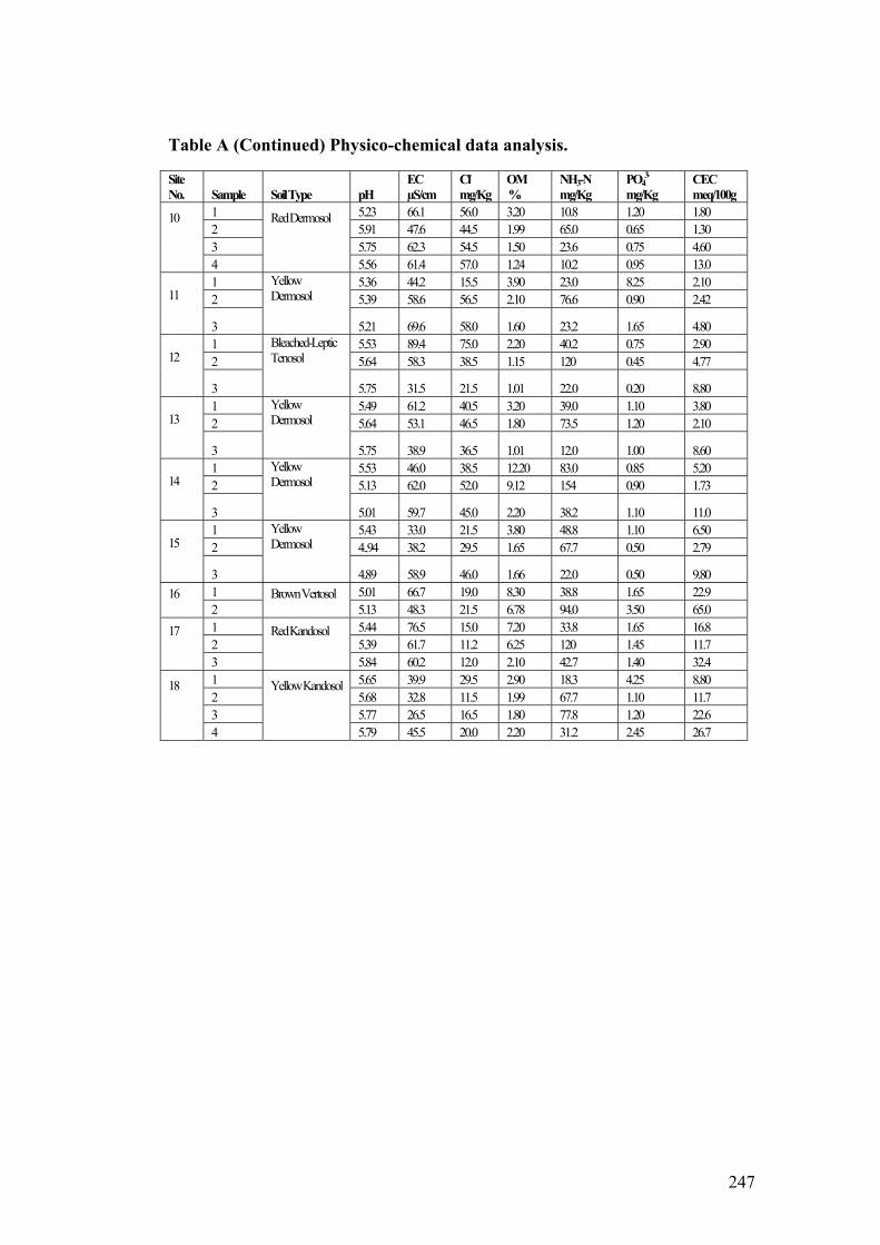
247

Table A (Continued) Physico-chemical data analysis.

Site No. Sample Soil Type pH

EC µS/cm

Cl- mg/Kg

OM %

NH3-N mg/Kg

PO43-

mg/Kg CEC meq/100g

1 5.23 66.1 56.0 3.20 10.8 1.20 1.80 2 5.91 47.6 44.5 1.99 65.0 0.65 1.30 3 5.75 62.3 54.5 1.50 23.6 0.75 4.60

10 4

Red Dermosol 5.56 61.4 57.0 1.24 10.2 0.95 13.0

1 5.36 44.2 15.5 3.90 23.0 8.25 2.10 2 5.39 58.6 56.5 2.10 76.6 0.90 2.42 11

3

Yellow Dermosol 5.21 69.6 58.0 1.60 23.2 1.65 4.80

1 5.53 89.4 75.0 2.20 40.2 0.75 2.90 2 5.64 58.3 38.5 1.15 120 0.45 4.77 12

3

Bleached-Leptic Tenosol 5.75 31.5 21.5 1.01 22.0 0.20 8.80

1 5.49 61.2 40.5 3.20 39.0 1.10 3.80 2 5.64 53.1 46.5 1.80 73.5 1.20 2.10 13

3

Yellow Dermosol 5.75 38.9 36.5 1.01 12.0 1.00 8.60

1 5.53 46.0 38.5 12.20 83.0 0.85 5.20 2 5.13 62.0 52.0 9.12 154 0.90 1.73 14

3

Yellow Dermosol 5.01 59.7 45.0 2.20 38.2 1.10 11.0

1 5.43 33.0 21.5 3.80 48.8 1.10 6.50 2 4..94 38.2 29.5 1.65 67.7 0.50 2.79 15

3

Yellow Dermosol 4.89 58.9 46.0 1.66 22.0 0.50 9.80

1 5.01 66.7 19.0 8.30 38.8 1.65 22.9 16 2

Brown Vertosol 5.13 48.3 21.5 6.78 94.0 3.50 65.0

1 5.44 76.5 15.0 7.20 33.8 1.65 16.8 2 5.39 61.7 11.2 6.25 120 1.45 11.7

17 3

Red Kandosol 5.84 60.2 12.0 2.10 42.7 1.40 32.4

1 5.65 39.9 29.5 2.90 18.3 4.25 8.80 2 5.68 32.8 11.5 1.99 67.7 1.10 11.7 3 5.77 26.5 16.5 1.80 77.8 1.20 22.6

18 4

Yellow Kandosol 5.79 45.5 20.0 2.20 31.2 2.45 26.7

248

Table A (Continued) Physico-chemical data analysis.

Site No. Sample Soil Type pH

EC µS/cm

Cl- mg/Kg

OM %

NH3-N mg/Kg

PO43-

mg/Kg CEC meq/100g

1 5.60 68.1 56.0 11.00 40.0 1.25 22.9 2 5.04 37.8 14.0 9.11 125 1.15 68.2 19

3

Yellow Kandosol 5.02 32.8 13.0 3.20 66.0 1.25 58.0

1 4.58 85.0 21.0 12.10 32.0 1.15 4.80 2 4.93 61.4 62.0 8.24 83.1 1.00 3.54 3 5.13 57.8 46.0 3.80 22.0 0.95 16.8

20 4

Red Vertosol 5.16 74.0 56.5 2.08 34.0 1.25 18.8

1 4.82 55.4 21.5 6.80 52.5 1.85 6.80 2 4.82 38.5 14.5 4.26 83.1 0.10 7.97 3 4.96 32.8 14.5 1.20 68.8 0.80 15.8

21 4

Yellow Kandosol 5.27 18.0 6.00 1.08 12.8 0.55 18.2

1 5.43 86.5 68.0 13.60 98.2 1.35 19.6 22 2

Yellow Kandosol 5.01 102 80.0 11.24 195 1.25 59.1

1 5.00 63.4 51.0 5.80 48.0 1.00 4.80 23 2

Gray Dermosol 5.35 91.1 55.5 2.90 167 2.25 16.3

24 1 Yellow Sodosol 4.65 22.1 10.0 6.13 142 1.70 59.1 1 4.36 66.7 17.0 10.20 48.0 3.10 8.02 2 4.65 91.6 62.5 9.75 148 0.90 14.8 3 4.74 84.1 70.0 3.93 111 1.50 86.6 4 4.57 88.4 74.5 1.60 44.6 1.25 88.8

25 5

Red Kandosol 4.68 79.0 53.0 11.20 47.9 1.30 33.8

1 4.89 77.0 68.0 9.83 35.2 1.25 39.8 2 5.06 70.0 58.0 7.79 142 1.25 14.8 26

3 Red Kandosol 4.51 56.4 43.0 3.98 76.6 0.85 75.0

1 5.14 88 80.0 8.90 48.7 1.60 22.1 2 4.98 66.2 53.0 7.26 181 1.85 82.5

27 3

Red Kandosol 4.60 53.3 48.0 1.70 68.2 1.65 88.6

1 4.60 90.6 22.5 5.80 88.0 0.90 14.8 2 4.98 63.0 62.0 2.14 106 1.00 33.4 3 4.60 37.7 28.0 1.80 40.6 1.60 38.8 4 5.14 48.0 46.5 1.60 22.8 1.10 44.2

28 5

Yellow Kandosol 4.45 109 100 1.20 21.4 1.10 36.2

1 4.86 33.0 20.0 4.86 66.8 11.8 2.40 29 2

Yellow Dermosol 5.19 68.5 58.5 2.93 181 2.35 5.19

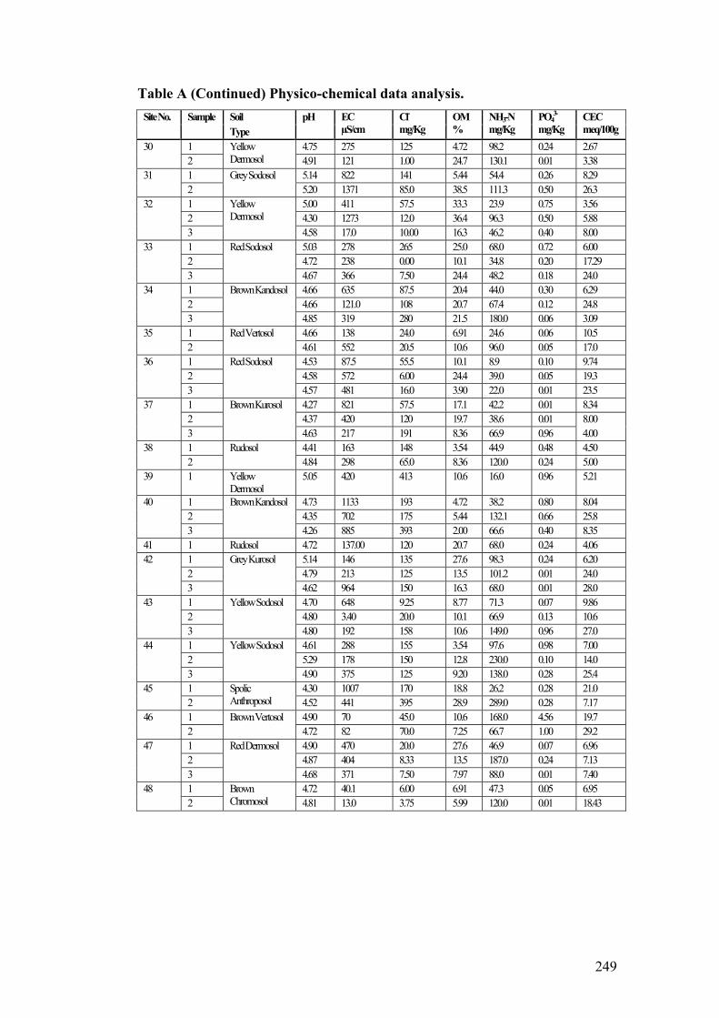
249

Table A (Continued) Physico-chemical data analysis. Soil Site No. Sample Type

pH EC µS/cm

Cl- mg/Kg

OM %

NH3-N mg/Kg

PO43-

mg/Kg CEC meq/100g

1 4.75 275 125 4.72 98.2 0.24 2.67 30 2

Yellow Dermosol 4.91 121 1.00 24.7 130.1 0.01 3.38

1 5.14 822 141 5.44 54.4 0.26 8.29 31 2

Grey Sodosol 5.20 1371 85.0 38.5 111.3 0.50 26.3

1 5.00 411 57.5 33.3 23.9 0.75 3.56 2 4.30 1273 12.0 36.4 96.3 0.50 5.88

32

3

Yellow Dermosol

4.58 17.0 10.00 16.3 46.2 0.40 8.00 1 5.03 278 265 25.0 68.0 0.72 6.00 2 4.72 238 0.00 10.1 34.8 0.20 17.29

33

3

Red Sodosol

4.67 366 7.50 24.4 48.2 0.18 24.0 1 4.66 635 87.5 20.4 44.0 0.30 6.29 2 4.66 121.0 108 20.7 67.4 0.12 24.8

34

3

Brown Kandosol

4.85 319 280 21.5 180.0 0.06 3.09 1 4.66 138 24.0 6.91 24.6 0.06 10.5 35 2

Red Vertosol 4.61 552 20.5 10.6 96.0 0.05 17.0

1 4.53 87.5 55.5 10.1 8.9 0.10 9.74 2 4.58 572 6.00 24.4 39.0 0.05 19.3

36

3

Red Sodosol

4.57 481 16.0 3.90 22.0 0.01 23.5 1 4.27 821 57.5 17.1 42.2 0.01 8.34 2 4.37 420 120 19.7 38.6 0.01 8.00

37

3

Brown Kurosol

4.63 217 191 8.36 66.9 0.96 4.00 1 4.41 163 148 3.54 44.9 0.48 4.50 38 2

Rudosol 4.84 298 65.0 8.36 120.0 0.24 5.00

39 1 Yellow Dermosol

5.05 420 413 10.6 16.0 0.96 5.21

1 4.73 1133 193 4.72 38.2 0.80 8.04 2 4.35 702 175 5.44 132.1 0.66 25.8

40

3

Brown Kandosol

4.26 885 393 2.00 66.6 0.40 8.35 41 1 Rudosol 4.72 137.00 120 20.7 68.0 0.24 4.06

1 5.14 146 135 27.6 98.3 0.24 6.20 2 4.79 213 125 13.5 101.2 0.01 24.0

42

3

Grey Kurosol

4.62 964 150 16.3 68.0 0.01 28.0 1 4.70 648 9.25 8.77 71.3 0.07 9.86 2 4.80 3.40 20.0 10.1 66.9 0.13 10.6

43

3

Yellow Sodosol

4.80 192 158 10.6 149.0 0.96 27.0 1 4.61 288 155 3.54 97.6 0.98 7.00 2 5.29 178 150 12.8 230.0 0.10 14.0

44

3

Yellow Sodosol

4.90 375 125 9.20 138.0 0.28 25.4 1 4.30 1007 170 18.8 26.2 0.28 21.0 45 2

Spolic Anthroposol 4.52 441 395 28.9 289.0 0.28 7.17

1 4.90 70 45.0 10.6 168.0 4.56 19.7 46 2

Brown Vertosol 4.72 82 70.0 7.25 66.7 1.00 29.2

1 4.90 470 20.0 27.6 46.9 0.07 6.96 2 4.87 404 8.33 13.5 187.0 0.24 7.13

47

3

Red Dermosol

4.68 371 7.50 7.97 88.0 0.01 7.40 1 4.72 40.1 6.00 6.91 47.3 0.05 6.95 48 2

Brown Chromosol 4.81 13.0 3.75 5.99 120.0 0.01 18.43

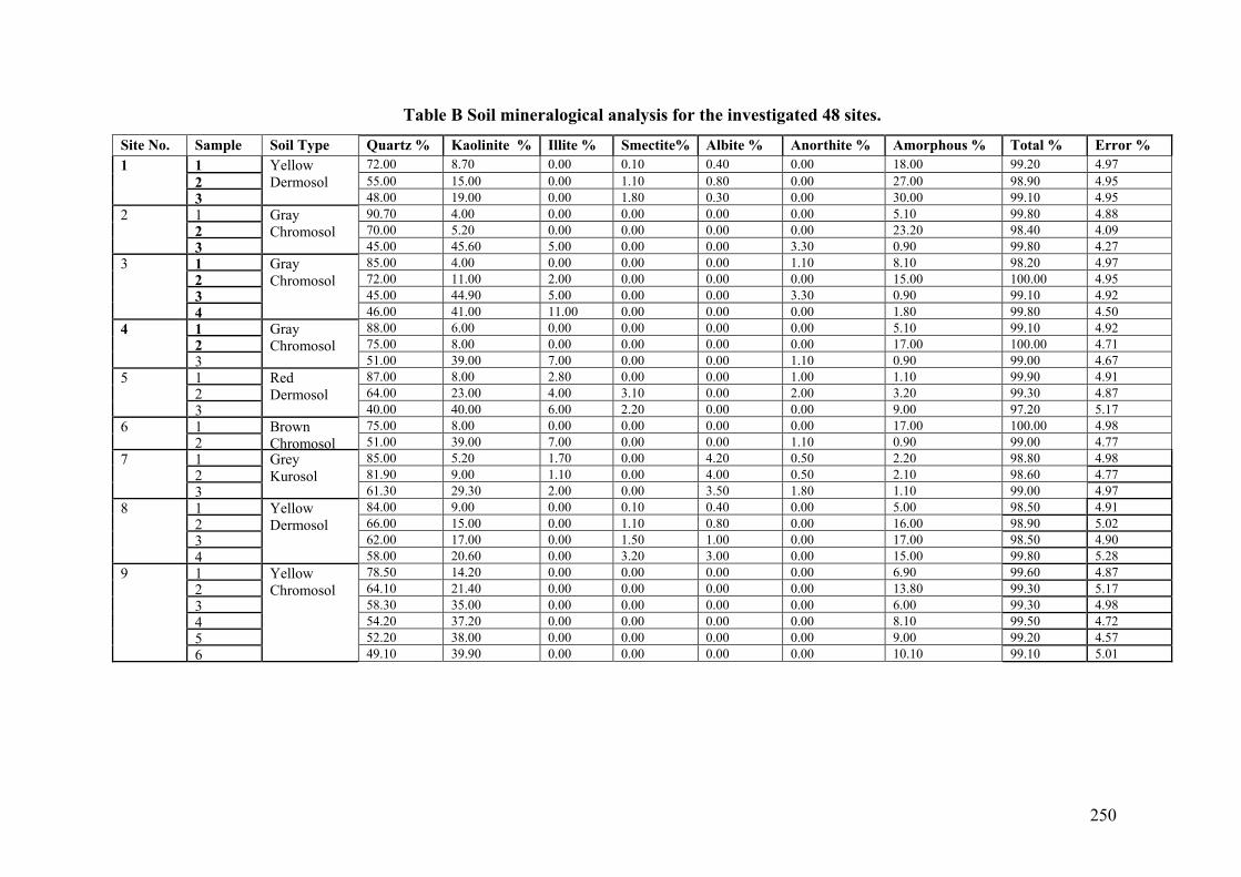
250

Table B Soil mineralogical analysis for the investigated 48 sites.

Site No. Sample Soil Type Quartz % Kaolinite % Illite % Smectite% Albite % Anorthite % Amorphous % Total % Error % 1 72.00 8.70 0.00 0.10 0.40 0.00 18.00 99.20 4.97 2 55.00 15.00 0.00 1.10 0.80 0.00 27.00 98.90 4.95

1

3

Yellow Dermosol

48.00 19.00 0.00 1.80 0.30 0.00 30.00 99.10 4.95 1 90.70 4.00 0.00 0.00 0.00 0.00 5.10 99.80 4.88 2 70.00 5.20 0.00 0.00 0.00 0.00 23.20 98.40 4.09

2

3

Gray Chromosol

45.00 45.60 5.00 0.00 0.00 3.30 0.90 99.80 4.27 1 85.00 4.00 0.00 0.00 0.00 1.10 8.10 98.20 4.97 2 72.00 11.00 2.00 0.00 0.00 0.00 15.00 100.00 4.95 3 45.00 44.90 5.00 0.00 0.00 3.30 0.90 99.10 4.92

3

4

Gray Chromosol

46.00 41.00 11.00 0.00 0.00 0.00 1.80 99.80 4.50 1 88.00 6.00 0.00 0.00 0.00 0.00 5.10 99.10 4.92 2 75.00 8.00 0.00 0.00 0.00 0.00 17.00 100.00 4.71

4

3

Gray Chromosol

51.00 39.00 7.00 0.00 0.00 1.10 0.90 99.00 4.67 1 87.00 8.00 2.80 0.00 0.00 1.00 1.10 99.90 4.91 2 64.00 23.00 4.00 3.10 0.00 2.00 3.20 99.30 4.87

5

3

Red Dermosol

40.00 40.00 6.00 2.20 0.00 0.00 9.00 97.20 5.17 1 75.00 8.00 0.00 0.00 0.00 0.00 17.00 100.00 4.98 6 2

Brown Chromosol 51.00 39.00 7.00 0.00 0.00 1.10 0.90 99.00 4.77

1 85.00 5.20 1.70 0.00 4.20 0.50 2.20 98.80 4.98 2 81.90 9.00 1.10 0.00 4.00 0.50 2.10 98.60 4.77

7

3

Grey Kurosol

61.30 29.30 2.00 0.00 3.50 1.80 1.10 99.00 4.97 1 84.00 9.00 0.00 0.10 0.40 0.00 5.00 98.50 4.91 2 66.00 15.00 0.00 1.10 0.80 0.00 16.00 98.90 5.02 3 62.00 17.00 0.00 1.50 1.00 0.00 17.00 98.50 4.90

8

4

Yellow Dermosol

58.00 20.60 0.00 3.20 3.00 0.00 15.00 99.80 5.28 1 78.50 14.20 0.00 0.00 0.00 0.00 6.90 99.60 4.87 2 64.10 21.40 0.00 0.00 0.00 0.00 13.80 99.30 5.17 3 58.30 35.00 0.00 0.00 0.00 0.00 6.00 99.30 4.98 4 54.20 37.20 0.00 0.00 0.00 0.00 8.10 99.50 4.72 5 52.20 38.00 0.00 0.00 0.00 0.00 9.00 99.20 4.57

9

6

Yellow Chromosol

49.10 39.90 0.00 0.00 0.00 0.00 10.10 99.10 5.01

251

Table B (Continued) Soil mineralogical analysis for the investigated 48 sites

Site No. Sample Soil Type Quartz %

Kaolinite %

Illite % Smectite% Albite % Anorthite % Amorphous % Total % Error %

1 84.00 8.00 5.00 0.00 0.00 1.00 1.10 99.10 4.88 2 54.00 32.00 3.10 3.10 0.00 3.90 3.20 99.30 4.72 3 40.00 40.00 6.00 2.20 0.00 0.00 9.00 97.20 4.87

10

4

Red Dermosol

41.00 38.00 7.00 5.20 0.00 0.00 8.00 99.20 4.57 1 76.00 10.10 0.00 0.10 0.40 0.00 12.00 98.60 4.95 2 71.00 17.00 0.00 1.10 0.80 0.00 10.00 99.90 4.88

11

3

Yellow Dermosol

59.00 22.00 0.00 4.00 2.00 0.00 12.00 99.00 4.72 1 88.00 4.00 0.00 0.00 1.00 0.00 6.20 99.20 4.57 2 71.00 12.00 0.00 0.00 1.70 0.00 14.20 98.90 5.01

12

3

Bleached-Leptic Tenosol

66.00 14.00 0.00 0.00 2.00 0.00 17.90 99.90 4.87 1 88.00 8.00 0.00 0.00 0.00 0.00 3.30 99.30 4.87 2 85.00 10.00 1.20 0.30 0.00 0.00 2.30 98.80 5.17

13

3

Yellow Dermosol

76.00 10.10 0.00 0.10 0.40 0.00 12.00 98.60 4.98 1 58.50 8.70 0.00 0.10 0.40 0.00 31.00 98.70 4.95 2 55.00 15.00 0.00 1.10 0.80 0.00 27.00 98.90 4.88

14

3

Yellow Dermosol

50.00 23.00 0.00 3.30 4.00 0.00 19.00 99.30 4.87 1 84.00 9.00 0.00 0.10 0.40 0.00 5.00 98.50 4.97 2 66.00 15.00 0.00 1.10 0.80 0.00 16.00 98.90 4.95

15

3

Yellow Dermosol

85.00 10.00 1.20 0.30 0.00 0.00 2.30 98.80 4.92 1 69.00 14.00 2.90 0.00 3.40 0.00 10.10 99.40 4.97 16 2

Brown Vertosol 55.40 37.00 1.70 0.30 3.40 0.20 1.30 99.30 4.88

1 81.00 7.00 7.80 0.00 0.00 0.00 1.60 97.40 4.37 2 61.00 23.00 9.00 3.50 0.70 0.00 2.10 99.30 4.91

17

3

Red Kandosol

46.10 36.00 9.10 0.00 8.50 0.00 0.00 99.70 5.02 1 87.00 5.00 4.00 0.00 0.00 0.00 2.10 98.10 4.97 2 61.00 15.00 18.00 0.00 0.00 0.00 4.20 98.20 4.95 3 56.00 26.00 16.00 0.00 0.00 0.00 1.10 99.10 5.17

18

4

Yellow Kandosol

51.30 31.00 16.10 0.00 0.00 0.00 1.30 99.70 4.98

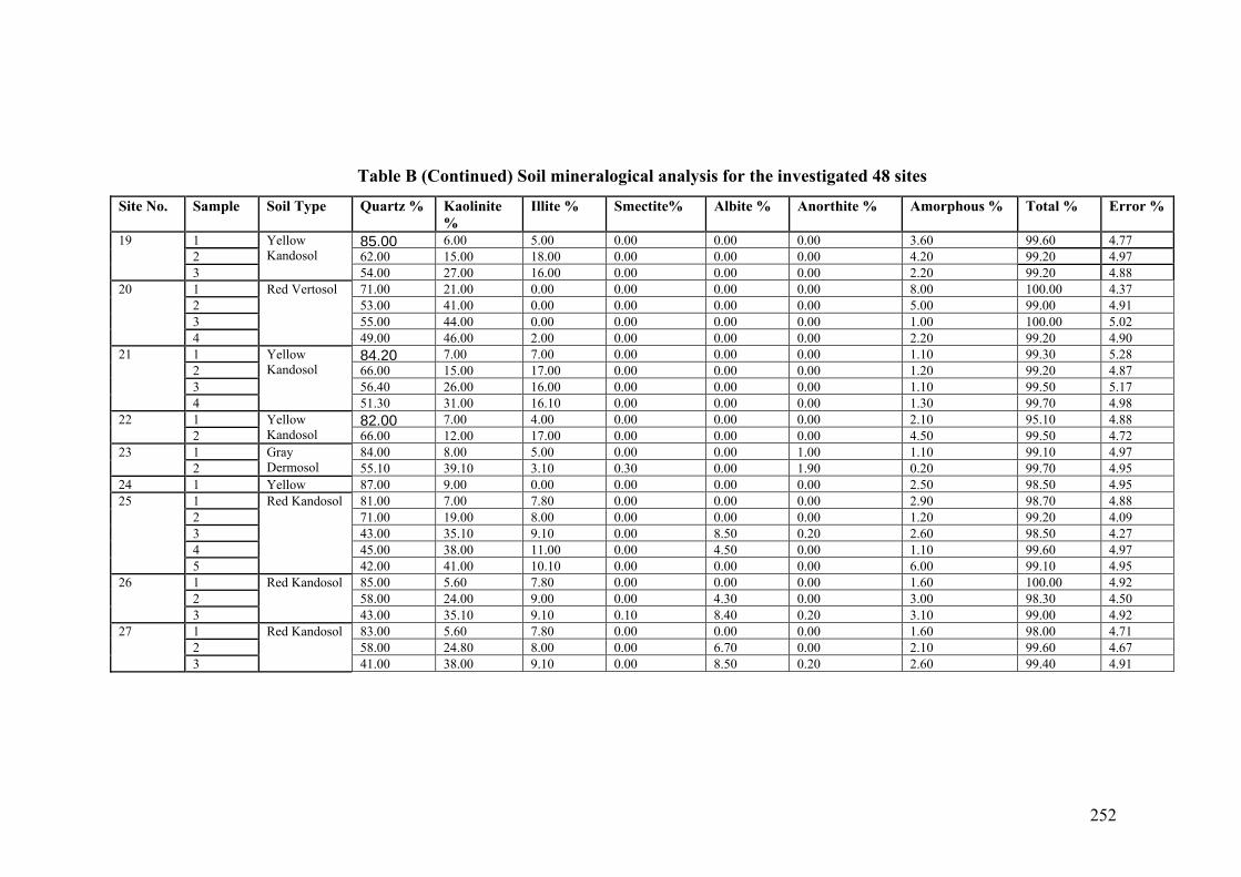
252


Site No. Sample Soil Type Quartz % Kaolinite %

Illite % Smectite% Albite % Anorthite % Amorphous % Total % Error %

1 85.00 6.00 5.00 0.00 0.00 0.00 3.60 99.60 4.77 2 62.00 15.00 18.00 0.00 0.00 0.00 4.20 99.20 4.97

19

3

Yellow Kandosol

54.00 27.00 16.00 0.00 0.00 0.00 2.20 99.20 4.88 1 71.00 21.00 0.00 0.00 0.00 0.00 8.00 100.00 4.37 2 53.00 41.00 0.00 0.00 0.00 0.00 5.00 99.00 4.91 3 55.00 44.00 0.00 0.00 0.00 0.00 1.00 100.00 5.02

20

4

Red Vertosol

49.00 46.00 2.00 0.00 0.00 0.00 2.20 99.20 4.90 1 84.20 7.00 7.00 0.00 0.00 0.00 1.10 99.30 5.28 2 66.00 15.00 17.00 0.00 0.00 0.00 1.20 99.20 4.87 3 56.40 26.00 16.00 0.00 0.00 0.00 1.10 99.50 5.17

21

4

Yellow Kandosol

51.30 31.00 16.10 0.00 0.00 0.00 1.30 99.70 4.98 1 82.00 7.00 4.00 0.00 0.00 0.00 2.10 95.10 4.88 22 2

Yellow Kandosol 66.00 12.00 17.00 0.00 0.00 0.00 4.50 99.50 4.72

1 84.00 8.00 5.00 0.00 0.00 1.00 1.10 99.10 4.97 23 2

Gray Dermosol 55.10 39.10 3.10 0.30 0.00 1.90 0.20 99.70 4.95

24 1 Yellow 87.00 9.00 0.00 0.00 0.00 0.00 2.50 98.50 4.95 1 81.00 7.00 7.80 0.00 0.00 0.00 2.90 98.70 4.88 2 71.00 19.00 8.00 0.00 0.00 0.00 1.20 99.20 4.09 3 43.00 35.10 9.10 0.00 8.50 0.20 2.60 98.50 4.27 4 45.00 38.00 11.00 0.00 4.50 0.00 1.10 99.60 4.97

25

5

Red Kandosol

42.00 41.00 10.10 0.00 0.00 0.00 6.00 99.10 4.95 1 85.00 5.60 7.80 0.00 0.00 0.00 1.60 100.00 4.92 2 58.00 24.00 9.00 0.00 4.30 0.00 3.00 98.30 4.50

26

3

Red Kandosol

43.00 35.10 9.10 0.10 8.40 0.20 3.10 99.00 4.92 1 83.00 5.60 7.80 0.00 0.00 0.00 1.60 98.00 4.71 2 58.00 24.80 8.00 0.00 6.70 0.00 2.10 99.60 4.67

27

3

Red Kandosol

41.00 38.00 9.10 0.00 8.50 0.20 2.60 99.40 4.91

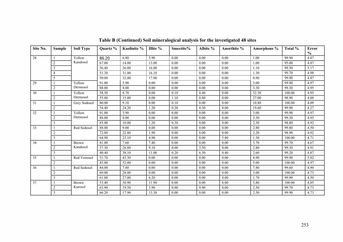
253


Site No. Sample Soil Type Quartz % Kaolinite % Illite % Smectite% Albite % Anorthite % Amorphous % Total % Error %

1 86.20 6.80 5.90 0.00 0.00 0.00 1.00 99.90 4.87 2 67.00 14.00 13.00 0.00 0.00 0.00 1.00 95.00 4.87 3 56.40 26.00 16.00 0.00 0.00 0.00 1.10 99.50 5.17 4 51.30 31.00 16.10 0.00 0.00 0.00 1.30 99.70 4.98

28

5

Yellow Kandosol

50.00 32.00 17.00 0.00 0.00 0.00 0.90 99.90 4.87 1 91.00 5.90 0.00 0.00 0.00 0.00 3.00 99.90 4.97 29 2

Yellow Dermosol 88.00 8.00 0.00 0.00 0.00 0.00 3.30 99.30 4.95

1 58.50 8.70 0.00 0.10 0.40 0.00 32.30 100.00 4.95 30 2

Yellow Dermosol 55.00 15.00 0.00 1.10 0.80 0.00 27.00 98.90 4.88

1 80.00 9.10 0.00 0.10 0.00 0.00 10.80 100.00 4.09 31 2

Grey Sodosol 54.40 24.20 1.20 0.20 0.30 0.00 19.60 99.90 4.27

1 91.00 5.90 0.00 0.00 0.00 0.00 3.00 99.90 4.97 2 88.00 8.00 0.00 0.00 0.00 0.00 3.30 99.30 4.95

32

3

Yellow Dermosol

85.00 10.00 1.20 0.30 0.00 0.00 2.30 98.80 4.92 1 88.00 9.00 0.00 0.00 0.00 0.00 2.80 99.80 4.50 2 72.00 22.80 1.90 0.00 0.00 0.00 2.20 98.90 4.92

33

3

Red Sodosol

64.90 23.10 4.90 0.00 0.00 5.80 1.30 100.00 4.71 1 81.00 7.60 7.40 0.00 0.00 0.00 3.70 99.70 4.67 2 57.30 26.80 9.10 0.00 3.30 0.00 2.80 99.30 4.91

34

3

Brown Kandosol

40.40 38.10 11.00 0.20 6.50 0.40 2.60 99.20 4.87 1 51.70 43.30 0.00 0.00 0.00 0.00 4.90 99.90 5.02 35 2

Red Vertosol 43.00 52.00 0.00 0.00 0.00 0.00 5.00 100.00 4.97

1 84.00 7.80 0.00 0.00 0.00 0.00 7.80 99.60 4.90 2 69.00 28.00 0.00 0.00 0.00 0.00 3.00 100.00 4.73

36

3

Red Sodosol

61.00 27.00 6.20 0.00 0.00 4.00 1.70 99.90 4.50 1 53.40 30.90 11.90 0.00 0.00 0.00 3.80 100.00 4.85 2 63.90 19.50 3.90 0.00 9.90 0.00 2.50 99.70 4.73

37

3

Brown Kurosol

66.20 17.90 13.30 0.00 0.00 0.00 2.50 99.90 4.73

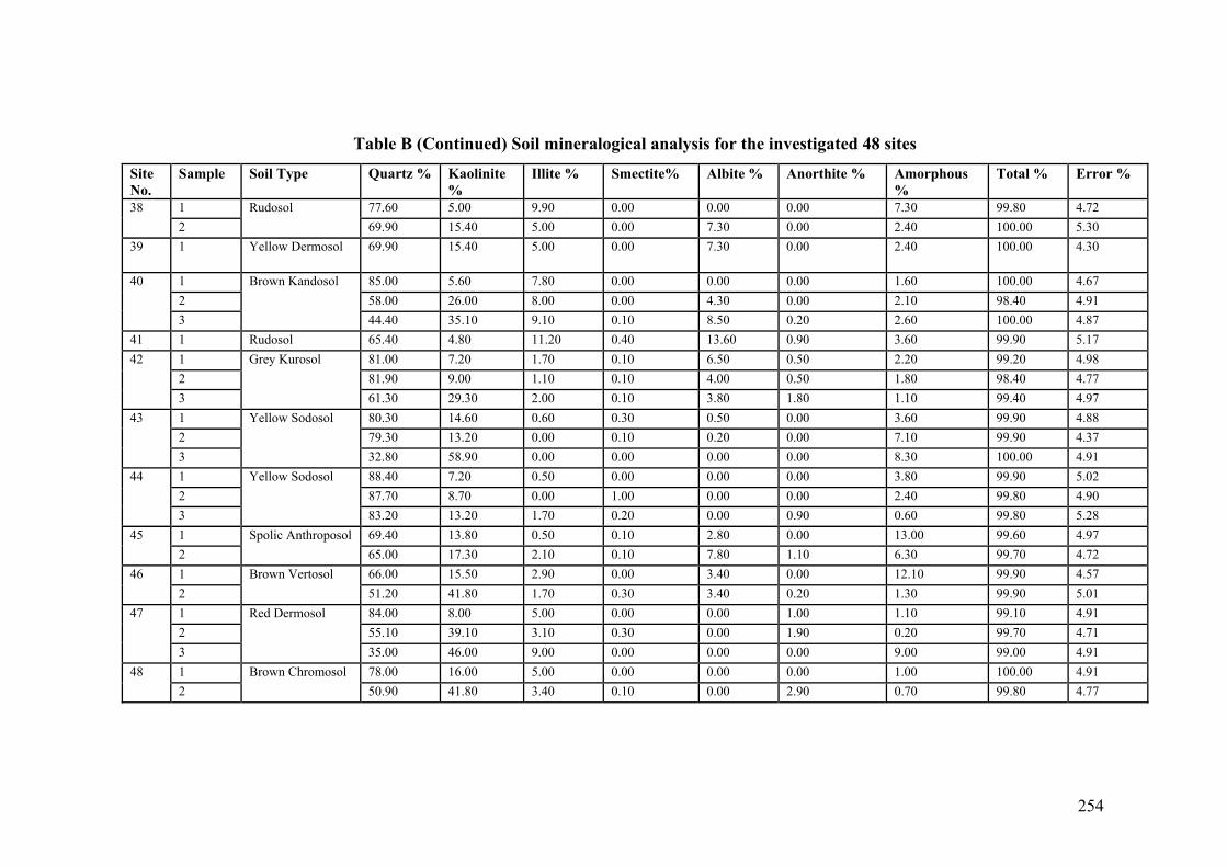
254


Site No.

Sample Soil Type Quartz % Kaolinite %

Illite % Smectite% Albite % Anorthite % Amorphous %

Total % Error %

1 77.60 5.00 9.90 0.00 0.00 0.00 7.30 99.80 4.72 38 2

Rudosol 69.90 15.40 5.00 0.00 7.30 0.00 2.40 100.00 5.30

39 1 Yellow Dermosol 69.90 15.40 5.00 0.00 7.30 0.00 2.40 100.00 4.30

1 85.00 5.60 7.80 0.00 0.00 0.00 1.60 100.00 4.67 2 58.00 26.00 8.00 0.00 4.30 0.00 2.10 98.40 4.91

40

3

Brown Kandosol

44.40 35.10 9.10 0.10 8.50 0.20 2.60 100.00 4.87 41 1 Rudosol 65.40 4.80 11.20 0.40 13.60 0.90 3.60 99.90 5.17

1 81.00 7.20 1.70 0.10 6.50 0.50 2.20 99.20 4.98 2 81.90 9.00 1.10 0.10 4.00 0.50 1.80 98.40 4.77

42

3

Grey Kurosol

61.30 29.30 2.00 0.10 3.80 1.80 1.10 99.40 4.97 1 80.30 14.60 0.60 0.30 0.50 0.00 3.60 99.90 4.88 2 79.30 13.20 0.00 0.10 0.20 0.00 7.10 99.90 4.37

43

3

Yellow Sodosol

32.80 58.90 0.00 0.00 0.00 0.00 8.30 100.00 4.91 1 88.40 7.20 0.50 0.00 0.00 0.00 3.80 99.90 5.02 2 87.70 8.70 0.00 1.00 0.00 0.00 2.40 99.80 4.90

44

3

Yellow Sodosol

83.20 13.20 1.70 0.20 0.00 0.90 0.60 99.80 5.28 1 69.40 13.80 0.50 0.10 2.80 0.00 13.00 99.60 4.97 45 2

Spolic Anthroposol 65.00 17.30 2.10 0.10 7.80 1.10 6.30 99.70 4.72

1 66.00 15.50 2.90 0.00 3.40 0.00 12.10 99.90 4.57 46 2

Brown Vertosol 51.20 41.80 1.70 0.30 3.40 0.20 1.30 99.90 5.01

1 84.00 8.00 5.00 0.00 0.00 1.00 1.10 99.10 4.91 2 55.10 39.10 3.10 0.30 0.00 1.90 0.20 99.70 4.71

47

3

Red Dermosol

35.00 46.00 9.00 0.00 0.00 0.00 9.00 99.00 4.91 1 78.00 16.00 5.00 0.00 0.00 0.00 1.00 100.00 4.91 48 2

Brown Chromosol 50.90 41.80 3.40 0.10 0.00 2.90 0.70 99.80 4.77

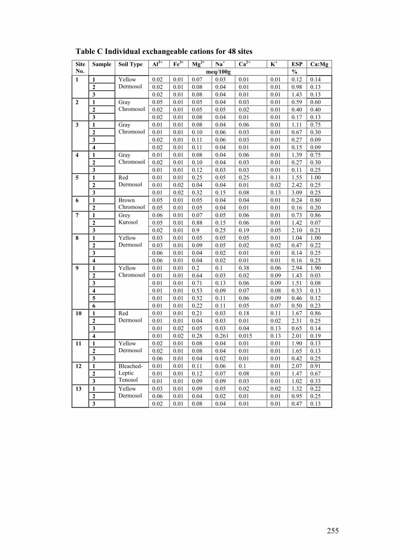
255

Table C Individual exchangeable cations for 48 sites Al3+ Fe3+ Mg2+ Na+ Ca2+ K+ ESP Ca:Mg Site

No. Sample Soil Type

meq/100g % 1 0.02 0.01 0.07 0.03 0.01 0.01 0.12 0.14 2 0.02 0.01 0.08 0.04 0.01 0.01 0.98 0.13

1

3

Yellow Dermosol

0.02 0.01 0.08 0.04 0.01 0.01 1.43 0.13 1 0.05 0.01 0.05 0.04 0.03 0.01 0.59 0.60 2 0.02 0.01 0.05 0.05 0.02 0.01 0.40 0.40

2

3

Gray Chromosol

0.02 0.01 0.08 0.04 0.01 0.01 0.17 0.13 1 0.01 0.01 0.08 0.04 0.06 0.01 1.11 0.75 2 0.01 0.01 0.10 0.06 0.03 0.01 0.67 0.30 3 0.02 0.01 0.11 0.06 0.03 0.01 0.27 0.09

3

4

Gray Chromosol

0.02 0.01 0.11 0.04 0.01 0.01 0.15 0.09 1 0.01 0.01 0.08 0.04 0.06 0.01 1.39 0.75 2 0.02 0.01 0.10 0.04 0.03 0.01 0.27 0.30

4

3

Gray Chromosol

0.01 0.01 0.12 0.03 0.03 0.01 0.11 0.25 1 0.01 0.01 0.25 0.05 0.25 0.11 1.55 1.00 2 0.01 0.02 0.04 0.04 0.01 0.02 2.42 0.25

5

3

Red Dermosol

0.01 0.02 0.32 0.15 0.08 0.13 3.09 0.25 1 0.05 0.01 0.05 0.04 0.04 0.01 0.24 0.80 6 2

Brown Chromosol 0.05 0.01 0.05 0.04 0.01 0.01 0.16 0.20

1 0.06 0.01 0.07 0.05 0.06 0.01 0.73 0.86 2 0.05 0.01 0.88 0.15 0.06 0.01 1.42 0.07

7

3

Grey Kurosol

0.02 0.01 0.9 0.25 0.19 0.05 2.10 0.21 1 0.03 0.01 0.05 0.05 0.05 0.01 1.04 1.00 2 0.03 0.01 0.09 0.05 0.02 0.02 0.47 0.22 3 0.06 0.01 0.04 0.02 0.01 0.01 0.14 0.25

8

4

Yellow Dermosol

0.06 0.01 0.04 0.02 0.01 0.01 0.16 0.25 1 0.01 0.01 0.2 0.1 0.38 0.06 2.94 1.90 2 0.01 0.01 0.64 0.03 0.02 0.09 1.43 0.03 3 0.01 0.01 0.71 0.13 0.06 0.09 1.51 0.08 4 0.01 0.01 0.53 0.09 0.07 0.08 0.33 0.13 5 0.01 0.01 0.52 0.11 0.06 0.09 0.46 0.12

9

6

Yellow Chromosol

0.01 0.01 0.22 0.11 0.05 0.07 0.50 0.23 1 0.01 0.01 0.21 0.03 0.18 0.11 1.67 0.86 2 0.01 0.01 0.04 0.03 0.01 0.02 2.31 0.25 3 0.01 0.02 0.05 0.03 0.04 0.13 0.65 0.14

10

4

Red Dermosol

0.01 0.02 0.28 0.261 0.015 0.13 2.01 0.19 1 0.02 0.01 0.08 0.04 0.01 0.01 1.90 0.13 2 0.02 0.01 0.08 0.04 0.01 0.01 1.65 0.13

11

3

Yellow Dermosol

0.06 0.01 0.04 0.02 0.01 0.01 0.42 0.25 1 0.01 0.01 0.11 0.06 0.1 0.01 2.07 0.91 2 0.01 0.01 0.12 0.07 0.08 0.01 1.47 0.67

12

3

Bleached-Leptic Tenosol 0.01 0.01 0.09 0.09 0.03 0.01 1.02 0.33

1 0.03 0.01 0.09 0.05 0.02 0.02 1.32 0.22 2 0.06 0.01 0.04 0.02 0.01 0.01 0.95 0.25

13

3

Yellow Dermosol

0.02 0.01 0.08 0.04 0.01 0.01 0.47 0.13

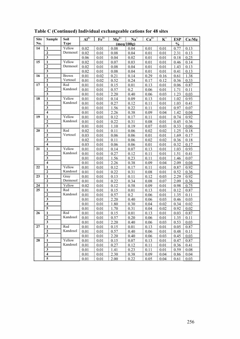
256

Table C (Continued) Individual exchangeable cations for 48 sites

Al3+ Fe3+ Mg2+ Na+ Ca2+ K+ ESP Ca:Mg Site No.

Sample Soil Type (meq/100g) %

1 0.02 0.01 0.08 0.04 0.01 0.01 0.77 0.13 2 0.02 0.01 0.08 0.04 0.01 0.01 2.31 0.13

14

3

Yellow Dermosol 0.06 0.01 0.04 0.02 0.01 0.01 0.18 0.25

1 0.02 0.01 0.07 0.03 0.01 0.01 0.46 0.14 2 0.02 0.01 0.08 0.04 0.01 0.01 1.43 0.13

15

3

Yellow Dermosol 0.02 0.01 0.08 0.04 0.01 0.01 0.41 0.13

1 0.01 0.02 0.21 0.14 0.29 0.16 0.61 1.38 16 2

Brown Vertosol 0.01 0.02 0.52 0.24 0.17 0.12 0.36 0.33

1 0.01 0.01 0.15 0.01 0.13 0.01 0.06 0.87 2 0.01 0.01 0.57 0.2 0.06 0.01 1.71 0.11

17

3

Red Kandosol 0.01 0.01 2.20 0.40 0.06 0.03 1.23 0.03

1 0.01 0.01 0.14 0.09 0.13 0.01 1.02 0.93 2 0.01 0.01 0.27 0.12 0.11 0.01 1.03 0.41 3 0.01 0.01 1.56 0.22 0.11 0.01 0.97 0.07

18

4

Yellow Kandosol

0.01 0.01 2.26 0.38 0.09 0.04 1.42 0.04 1 0.01 0.01 0.12 0.17 0.11 0.01 0.74 0.92 2 0.01 0.01 0.22 0.31 0.08 0.01 0.45 0.36

19

3

Yellow Kandosol

0.01 0.01 1.10 0.19 0.07 0.03 0.33 0.06 1 0.02 0.01 0.11 0.06 0.02 0.02 1.25 0.18 2 0.03 0.01 0.06 0.06 0.01 0.01 1.69 0.17 3 0.02 0.01 0.11 0.06 0.02 0.02 0.36 0.18

20

4

Red Vertosol

0.03 0.01 0.06 0.06 0.01 0.01 0.32 0.17 1 0.01 0.01 0.14 0.07 0.13 0.01 1.03 0.93 2 0.01 0.01 0.27 0.12 0.11 0.01 1.51 0.41 3 0.01 0.01 1.56 0.23 0.11 0.01 1.46 0.07

21

4

Yellow Kandosol

0.01 0.01 2.26 0.38 0.09 0.04 2.09 0.04 1 0.01 0.01 0.12 0.17 0.11 0.01 0.87 0.92 22 2

Yellow Kandosol 0.01 0.01 0.22 0.31 0.08 0.01 0.52 0.36

1 0.01 0.01 0.13 0.11 0.12 0.03 2.29 0.92 23 2

Gray Dermosol 0.01 0.01 0.22 0.34 0.08 0.07 2.09 0.36

24 1 Yellow 0.02 0.01 0.12 0.58 0.09 0.01 0.98 0.75 1 0.01 0.01 0.15 0.01 0.13 0.01 0.12 0.87 2 0.01 0.01 0.57 0.2 0.06 0.01 1.35 0.11 3 0.01 0.01 2.20 0.40 0.06 0.03 0.46 0.03 4 0.01 0.01 1.80 0.30 0.04 0.02 0.34 0.02

25

5

Red Kandosol

0.01 0.01 1.70 0.31 0.04 0.02 0.92 0.02 1 0.01 0.01 0.15 0.01 0.13 0.01 0.03 0.87 2 0.01 0.01 0.57 0.20 0.06 0.01 1.35 0.11

26

3

Red Kandosol

0.01 0.01 2.20 0.40 0.06 0.03 0.53 0.03 1 0.01 0.01 0.15 0.01 0.13 0.01 0.05 0.87 2 0.01 0.01 0.57 0.40 0.06 0.01 0.48 0.11

27

3

Red Kandosol

0.01 0.01 2.20 0.40 0.06 0.03 0.45 0.03 1 0.01 0.01 0.15 0.07 0.13 0.01 0.47 0.87 2 0.01 0.01 0.27 0.12 0.11 0.01 0.36 0.41 3 0.01 0.01 1.41 0.23 0.11 0.01 0.59 0.08 4 0.01 0.01 2.30 0.38 0.09 0.04 0.86 0.04

28

5

Yellow Kandosol

0.01 0.01 2.00 0.22 0.05 0.04 0.61 0.03

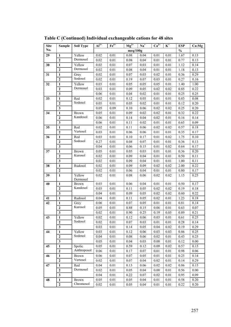
257

Table C (Continued) Individual exchangeable cations for 48 sites Al3+ Fe#+ Mg2+ Na+ Ca2+ K+ ESP Ca:Mg Site

No. Sample Soil Type

meq/100g % 1 0.02 0.01 0.08 0.04 0.01 0.01 1.67 0.13 29 2

Yellow Dermosol 0.02 0.01 0.08 0.04 0.01 0.01 0.77 0.13

1 0.02 0.01 0.07 0.03 0.01 0.01 1.12 0.14 30 2

Yellow Dermosol 0.02 0.01 0.08 0.04 0.01 0.01 1.18 0.13

1 0.02 0.01 0.07 0.03 0.02 0.01 0.36 0.29 31 2

Grey Sodosol 0.02 0.01 0.19 0.07 0.03 0.01 0.27 0.16

1 0.03 0.01 0.05 0.05 0.05 0.01 1.40 1.00 2 0.03 0.01 0.09 0.05 0.02 0.02 0.85 0.22

32

3

Yellow Dermosol

0.06 0.01 0.04 0.02 0.01 0.01 0.25 0.25 1 0.02 0.01 0.12 0.05 0.01 0.01 0.83 0.08 2 0.05 0.01 0.05 0.02 0.01 0.01 0.12 0.20

33

3

Red Sodosol

0.05 0.09 0.10 0.06 0.02 0.02 0.25 0.20 1 0.05 0.01 0.09 0.02 0.02 0.01 0.32 0.22 2 0.06 0.01 0.14 0.04 0.02 0.01 0.16 0.14

34

3

Brown Kandosol

0.06 0.01 0.11 0.02 0.01 0.01 0.65 0.09 1 0.02 0.01 0.11 0.06 0.02 0.02 0.57 0.18 35 2

Red Vertosol 0.03 0.01 0.06 0.06 0.01 0.01 0.35 0.17

1 0.03 0.01 0.10 0.17 0.01 0.02 1.75 0.10 2 0.27 0.01 0.08 0.07 0.01 0.01 0.36 0.13

36

3

Red Sodosol

0.04 0.01 0.06 0.15 0.01 0.02 0.64 0.17 1 0.05 0.01 0.05 0.03 0.01 0.01 0.36 0.20 2 0.02 0.01 0.09 0.04 0.01 0.01 0.50 0.11

37

3

Brown Kurosol

0.02 0.01 0.09 0.04 0.01 0.01 1.00 0.11 1 0.02 0.01 0.09 0.09 0.02 0.02 2.00 0.22 38 2

Rudosol 0.02 0.01 0.06 0.04 0.01 0.01 0.80 0.17

39 1 Yellow Dermosol

0.02 0.01 0.08 0.06 0.02 0.02 1.15 0.25

1 0.03 0.01 0.06 0.04 0.01 0.01 0.50 0.17 2 0.03 0.01 0.11 0.05 0.02 0.02 0.19 0.18

40

3

Brown Kandosol

0.04 0.01 0.09 0.05 0.02 0.02 0.60 0.22 41 1 Rudosol 0.04 0.01 0.11 0.05 0.02 0.01 1.23 0.18

1 0.06 0.01 0.07 0.05 0.01 0.01 0.81 0.14 2 0.05 0.01 0.88 0.15 0.06 0.01 0.63 0.07

42

3

Grey Kurosol

0.02 0.01 0.90 0.25 0.19 0.05 0.89 0.21 1 0.02 0.01 0.12 0.06 0.03 0.01 0.61 0.25 2 0.02 0.01 0.07 0.03 0.01 0.01 0.28 0.14

43

3

Yellow Sodosol

0.03 0.01 0.14 0.05 0.04 0.02 0.19 0.29 1 0.03 0.01 0.12 0.06 0.03 0.03 0.86 0.25 2 0.04 0.01 0.08 0.06 0.02 0.01 0.43 0.25

44

3

Yellow Sodosol

0.05 0.01 0.04 0.03 0.00 0.01 0.12 0.00 1 0.05 0.01 0.59 0.12 0.09 0.02 0.57 0.15 45 2

Spolic Anthroposol 0.06 0.01 0.17 0.07 0.01 0.01 0.98 0.06

1 0.06 0.01 0.07 0.05 0.01 0.01 0.25 0.14 46 2

Brown Vertosol 0.02 0.01 0.07 0.04 0.02 0.01 0.14 0.29

1 0.04 0.01 0.13 0.06 0.02 0.02 0.86 0.15 2 0.02 0.01 0.05 0.04 0.00 0.01 0.56 0.00

47

3

Red Dermosol

0.04 0.01 0.22 0.07 0.02 0.01 0.95 0.09 1 0.05 0.01 0.05 0.04 0.01 0.01 0.58 0.20 48 2

Brown Chromosol 0.02 0.01 0.05 0.04 0.01 0.01 0.22 0.20

258

Appendix B

Experimental Columns Data

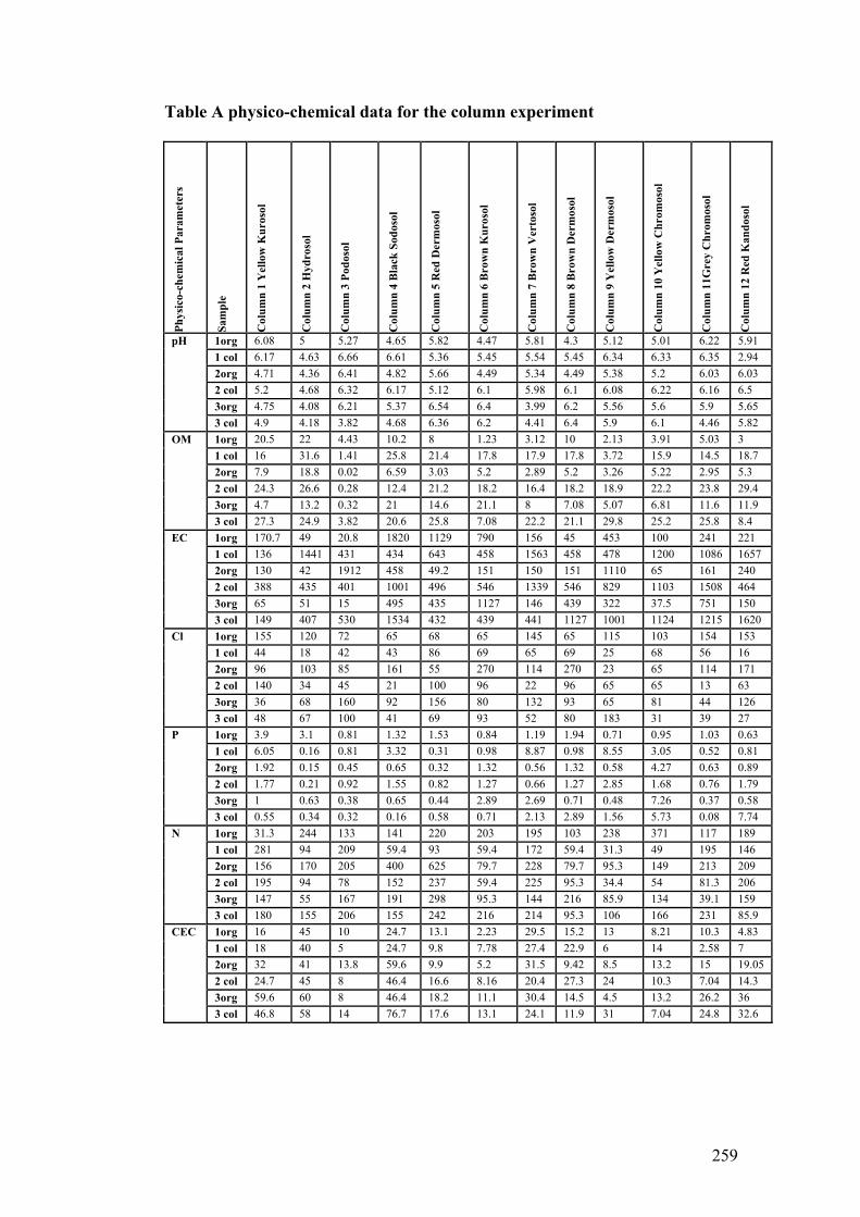
259

Table A physico-chemical data for the column experiment

Phys

ico-

chem

ical

Par

amet

ers

Sam

ple

Col

umn

1 Y

ello

w K

uros

ol

Col

umn

2 H

ydro

sol

Col

umn

3 Po

doso

l

Col

umn

4 B

lack

Sod

osol

Col

umn

5 R

ed D

erm

osol

Col

umn

6 B

row

n K

uros

ol

Col

umn

7 B

row

n V

erto

sol

Col

umn

8 B

row

n D

erm

osol

Col

umn

9 Y

ello

w D

erm

osol

Col

umn

10 Y

ello

w C

hrom

osol

Col

umn

11G

rey

Chr

omos

ol

Col

umn

12 R

ed K

ando

sol

1org 6.08 5 5.27 4.65 5.82 4.47 5.81 4.3 5.12 5.01 6.22 5.91 1 col 6.17 4.63 6.66 6.61 5.36 5.45 5.54 5.45 6.34 6.33 6.35 2.94 2org 4.71 4.36 6.41 4.82 5.66 4.49 5.34 4.49 5.38 5.2 6.03 6.03 2 col 5.2 4.68 6.32 6.17 5.12 6.1 5.98 6.1 6.08 6.22 6.16 6.5 3org 4.75 4.08 6.21 5.37 6.54 6.4 3.99 6.2 5.56 5.6 5.9 5.65

pH

3 col 4.9 4.18 3.82 4.68 6.36 6.2 4.41 6.4 5.9 6.1 4.46 5.82 1org 20.5 22 4.43 10.2 8 1.23 3.12 10 2.13 3.91 5.03 3 1 col 16 31.6 1.41 25.8 21.4 17.8 17.9 17.8 3.72 15.9 14.5 18.7 2org 7.9 18.8 0.02 6.59 3.03 5.2 2.89 5.2 3.26 5.22 2.95 5.3 2 col 24.3 26.6 0.28 12.4 21.2 18.2 16.4 18.2 18.9 22.2 23.8 29.4 3org 4.7 13.2 0.32 21 14.6 21.1 8 7.08 5.07 6.81 11.6 11.9

OM

3 col 27.3 24.9 3.82 20.6 25.8 7.08 22.2 21.1 29.8 25.2 25.8 8.4 1org 170.7 49 20.8 1820 1129 790 156 45 453 100 241 221 1 col 136 1441 431 434 643 458 1563 458 478 1200 1086 1657 2org 130 42 1912 458 49.2 151 150 151 1110 65 161 240 2 col 388 435 401 1001 496 546 1339 546 829 1103 1508 464 3org 65 51 15 495 435 1127 146 439 322 37.5 751 150

EC

3 col 149 407 530 1534 432 439 441 1127 1001 1124 1215 1620 1org 155 120 72 65 68 65 145 65 115 103 154 153 1 col 44 18 42 43 86 69 65 69 25 68 56 16 2org 96 103 85 161 55 270 114 270 23 65 114 171 2 col 140 34 45 21 100 96 22 96 65 65 13 63 3org 36 68 160 92 156 80 132 93 65 81 44 126

Cl

3 col 48 67 100 41 69 93 52 80 183 31 39 27 1org 3.9 3.1 0.81 1.32 1.53 0.84 1.19 1.94 0.71 0.95 1.03 0.63 1 col 6.05 0.16 0.81 3.32 0.31 0.98 8.87 0.98 8.55 3.05 0.52 0.81 2org 1.92 0.15 0.45 0.65 0.32 1.32 0.56 1.32 0.58 4.27 0.63 0.89 2 col 1.77 0.21 0.92 1.55 0.82 1.27 0.66 1.27 2.85 1.68 0.76 1.79 3org 1 0.63 0.38 0.65 0.44 2.89 2.69 0.71 0.48 7.26 0.37 0.58

P

3 col 0.55 0.34 0.32 0.16 0.58 0.71 2.13 2.89 1.56 5.73 0.08 7.74 1org 31.3 244 133 141 220 203 195 103 238 371 117 189 1 col 281 94 209 59.4 93 59.4 172 59.4 31.3 49 195 146 2org 156 170 205 400 625 79.7 228 79.7 95.3 149 213 209 2 col 195 94 78 152 237 59.4 225 95.3 34.4 54 81.3 206 3org 147 55 167 191 298 95.3 144 216 85.9 134 39.1 159

N

3 col 180 155 206 155 242 216 214 95.3 106 166 231 85.9 1org 16 45 10 24.7 13.1 2.23 29.5 15.2 13 8.21 10.3 4.83 1 col 18 40 5 24.7 9.8 7.78 27.4 22.9 6 14 2.58 7 2org 32 41 13.8 59.6 9.9 5.2 31.5 9.42 8.5 13.2 15 19.05 2 col 24.7 45 8 46.4 16.6 8.16 20.4 27.3 24 10.3 7.04 14.3 3org 59.6 60 8 46.4 18.2 11.1 30.4 14.5 4.5 13.2 26.2 36

CEC

3 col 46.8 58 14 76.7 17.6 13.1 24.1 11.9 31 7.04 24.8 32.6

260

Table B Soil columns mineralogy Column Sample Quartz

% Kaolinite %

Illite % Smectite %

Albite % Anorthite %

Amorphous %

Total % Error %

1org 60.3 20.5 0 0 18.3 0 0.73 99.8 4.2 1 col 68.4 28.2 0 0.9 0 0 1.98 99.5 4.3 2org 29.3 42.4 0 3 24 0 1.03 99.7 4.22 2 col 42 23.2 0 0 32 0 2.57 99.8 4.2 3org 39.8 21 0 7.8 30.4 0 0.85 99.9 4.2

1

3 col 38.9 20.1 0 6.8 34.1 0 0 99.9 4.25 1org 13.8 57.4 27 0 0 0 1.59 99.8 4.33 1 col 10.4 76 12 0 0 0 1.42 99.8 4.67 2org 9.1 67.1 21.4 0 0 0 2.19 99.8 4.27 2 col 23.6 61.5 9.4 0 0 0 5.08 99.6 4.86 3org 21.6 66 0 10.4 0 0 1.26 99.3 4.65

2

3 col 21.4 65.3 0 9.8 0 0 3.33 99.8 4.19 1org 94.1 3.3 0 0 0 0.1 2.07 99.6 4.07 1 col 86.7 0 0 0 0 2.6 10.7 100 5.13 2org 95.9 0 0 0 0.3 0 3.56 99.8 3.77 2 col 96.3 0 0 0 0 2.1 1.44 99.8 4.96 3org 89.9 3.4 0 0 0 0.5 5.98 99.8 4.34

3

3 col 83.7 0 0 0 1.6 14.4 0.15 99.9 5.43 1org 68.9 16.5 0 0 4.4 8.2 2 100 4.83 1 col 29.3 42.2 0 3 24 0 1.4 99.9 4.22 2org 68.4 28.2 0 0.2 0 0 2.2 99 4.55 2 col 39.8 21 0 7.8 29 0 1.1 98.7 4.52 3org 38.9 20.1 0 6.1 34.1 0 0 99.2 4.52

4

3 col 55.3 16.2 0 9.3 13.9 4.4 0.9 100 4.91

261

Table B (Continue) Soil columns mineralogy Column Sample Quartz % Kaolinite % Illite % Smectite % Albite % Anorthite % Amorphous % Total % Error %

1org 75 2 0 0 3.8 0 18.9 99.7 4.38 1col 58.4 5 6.8 0 21 3.8 4.86 99.9 5.95 2org 76.9 3.9 3.7 0 2.7 0 12.7 99.9 4.52 2col 55.4 10.9 6.2 0 0 0 27.5 100 5.02 3org 51.4 39.1 0 0 5.5 0 1.3 97.3 4.91

5

3col 55 36.5 4.9 0 0 0 2.6 99 4.32 1org 61.4 23.3 4.6 0 2.6 2.1 5.89 99.9 3.91 1 col 43.8 21.5 4.1 0 3.1 2.3 25.1 99.9 4.33 2org 75.4 14.1 4.2 0 3.6 1.6 0.92 99.8 3.84 2 col 63.1 11.8 4 0 3.2 1.65 16.2 99.9 4.01 3org 64.3 24 3.8 0 6.2 1.6 0 99.9 4.23

6

3 col 51.9 13.6 3.6 0 3.9 1.5 25.5 100 4.1 1org 82 12 0 0 0.4 0 5.2 99.6 5.32 1 col 78.2 15.6 0 0 1.6 0 4.4 99.8 4.83 2org 75.7 19.7 0 0 1.3 0 2.5 99.2 4 2 col 70.3 16.3 0 0 9.6 0 3.5 99.7 4.94 3org 55.8 43.1 0 0 0.3 0 0.3 99.5 4.89

7

3 col 58.8 40 0 0 0 0 1 99.8 4.88 1org 87.1 11.3 1.1 0 0 0 0.43 99.9 4.23 1 col 43.8 21.5 4.1 0 3.1 2.3 25.1 99.9 4.33 2org 75.4 14.1 4.2 0 3.6 1.6 0.92 99.8 3.84 2 col 42.5 27.1 4.01 0 3 2.2 20.2 99 4.8 3org 64.3 24 3.8 0 6.2 1.6 0 99.9 4.23

8

3 col 51.9 13.6 3.6 0 3.9 1.5 25.5 100 4.1

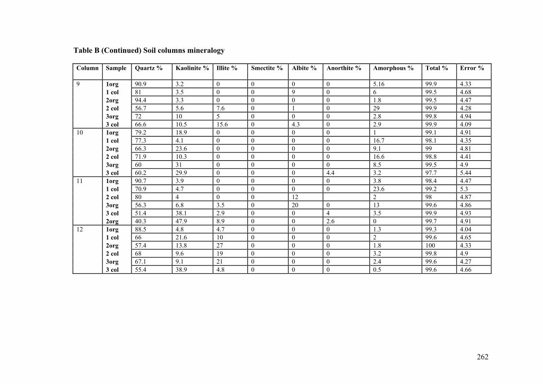
262

Table B (Continued) Soil columns mineralogy Column Sample Quartz % Kaolinite % Illite % Smectite % Albite % Anorthite % Amorphous % Total % Error %

1org 90.9 3.2 0 0 0 0 5.16 99.9 4.33 1 col 81 3.5 0 0 9 0 6 99.5 4.68 2org 94.4 3.3 0 0 0 0 1.8 99.5 4.47 2 col 56.7 5.6 7.6 0 1 0 29 99.9 4.28 3org 72 10 5 0 0 0 2.8 99.8 4.94

9

3 col 66.6 10.5 15.6 0 4.3 0 2.9 99.9 4.09 1org 79.2 18.9 0 0 0 0 1 99.1 4.91 1 col 77.3 4.1 0 0 0 0 16.7 98.1 4.35 2org 66.3 23.6 0 0 0 0 9.1 99 4.81 2 col 71.9 10.3 0 0 0 0 16.6 98.8 4.41 3org 60 31 0 0 0 0 8.5 99.5 4.9

10

3 col 60.2 29.9 0 0 0 4.4 3.2 97.7 5.44 1org 90.7 3.9 0 0 0 0 3.8 98.4 4.47 1 col 70.9 4.7 0 0 0 0 23.6 99.2 5.3 2 col 80 4 0 0 12 2 98 4.87 3org 56.3 6.8 3.5 0 20 0 13 99.6 4.86 3 col 51.4 38.1 2.9 0 0 4 3.5 99.9 4.93

11

2org 40.3 47.9 8.9 0 0 2.6 0 99.7 4.91 1org 88.5 4.8 4.7 0 0 0 1.3 99.3 4.04 1 col 66 21.6 10 0 0 0 2 99.6 4.65 2org 57.4 13.8 27 0 0 0 1.8 100 4.33 2 col 68 9.6 19 0 0 0 3.2 99.8 4.9 3org 67.1 9.1 21 0 0 0 2.4 99.6 4.27

12

3 col 55.4 38.9 4.8 0 0 0 0.5 99.6 4.66

263

Table C Columns individual cations analysis Column Sample Al3+ Fe3+ Mg2+ Na+ Ca2+ K+ ECEC ESP

meq/100g

Ca:Mg

meq/100g % 1org 0.09 0.04 0.54 0.13 0.54 0.15 1 27.2 0.81 1 col 0.00 0.06 0.36 0.2 0.56 0.28 1.53 27.9 1.12 2org 0.2 0.00 1.04 0.35 0.09 0.04 0.09 30.4 1.08 2 col 0.02 0.02 0.37 0.15 0.11 0.04 0.29 13.4 0.60 3org 0.65 0.00 1.68 0.54 0.06 0.09 0.04 47.5 0.90

1 3 col 0.19 0.01 1.16 0.74 0.04 0.02 0.04 39.2 1.57 1org 0.01 0.00 0.39 0.13 0.56 0.11 1.44 45.4 0.30 1 col 0.01 0.01 0.06 0.20 0.11 0.02 1.74 49.4 0.50 2org 0.00 0.00 0.09 0.10 0.17 0.07 1.92 39.0 0.18 2 col 0.00 0.00 0.13 0.11 0.22 0.00 1.70 21.6 0.24 3org 0.01 0.00 0.05 0.04 0.06 0.03 1.26 60.7 0.07





6 3 col 0.00 0.00 0.30 0.15 0.02 0.03 0.07 0.51 1.37

264

Table C (Continued) Columns individual cations analysis Column Sample Al#+ Fe3+ Mg2+ Na+ Ca2+ K+ ECEC ESP meq/100g

Ca:Mg

meq/100g % 1org 0.01 0.00 0.22 0.14 0.33 0.16 1.46 17.2 0.47 1 col 0.02 0.00 0.13 0.22 0.13 0.07 1.00 11.4 2.11 2org 0.01 0.00 0.52 0.24 0.17 0.12 0.33 21.2 1.35 2 col 0.00 0.00 0.15 0.10 0.05 0.06 0.36 7.1 0.31 3org 0.00 0.00 0.81 0.31 0.03 0.06 0.04 24.2 0.98





11 3 col 0.00 0.00 0.63 0.66 0.03 0.01 0.05 13.3 2.66 1org 0.00 0.00 0.15 0.09 0.07 0.01 0.48 3.27 1.95 1col 0.01 0.00 0.12 0.18 0.04 0.00 0.31 3.48 2.63 2org 0.01 0.00 0.53 0.19 0.06 0.01 0.11 8.10 2.14 2 col 0.00 0.00 0.61 0.15 0.03 0.00 0.04 7.77 1.03 3org 0.00 0.00 2.59 0.38 0.06 0.04 0.02 30.8 1.04

12 3 col 0.00 0.00 0.81 0.13 0.03 0.01 0.04 9.83 0.59

265

Table D1 Effluent data analysis for soil column No. 1

Column 1 (YellowKurosol) Sampling

Point Dates No. of

Samples Effluent Added (mL)

pH NH3-N mg/L

PO43+

mg/L EC

µS/cm TCOD mg/L

Nitrogen Removal

%

Phos. Removal

%

EC Reduction

%

TCOD removal

% Initial Average 6 5000 8 8.8 1.00 980 192

1 12/12/2002 1 120 7.5 4.1 0.08 509 67 53 92 48 65 1 15/01/2003 1 120 6.9 3.8 0.08 520 65 57 92 47 66 1 25/01/2003 1 120 7.1 3.9 0.09 518 48 56 91 47 75 1 28/02/2003 1 120 5.5 2.9 0.07 480 60 56 93 51 69 2 13/12/2002 1 40 6.6 0.7 0.01 483 37 92 99 51 81 2 25/03/2003 1 60 5.8 0.9 0.01 468 25 69 99 52 87 2 12/04/2003 1 40 5.9 1.1 0.02 388 19 88 98 60 90 2 31/07/2003 1 60 6.2 1.0 0.03 276 14 76 97 72 93 2 7/09/2003 1 100 6.5 1.2 0.04 148 10 68 96 85 95

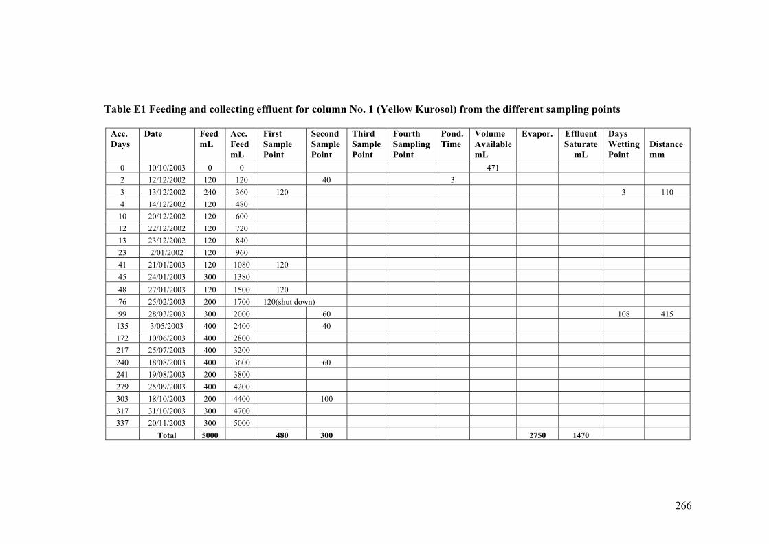
266

Table E1 Feeding and collecting effluent for column No. 1 (Yellow Kurosol) from the different sampling points

Acc. Days

Date

Feed mL

Acc. Feed mL

First Sample Point

Second Sample Point

Third Sample Point

Fourth Sampling Point

Pond. Time

Volume AvailablemL

Evapor.

Effluent Saturate

mL

Days WettingPoint

Distance mm

0 10/10/2003 0 0 471 2 12/12/2002 120 120 40 3 3 13/12/2002 240 360 120 3 110 4 14/12/2002 120 480 10 20/12/2002 120 600 12 22/12/2002 120 720 13 23/12/2002 120 840 23 2/01/2002 120 960 41 21/01/2003 120 1080 120 45 24/01/2003 300 1380 48 27/01/2003 120 1500 120 76 25/02/2003 200 1700 120(shut down) 99 28/03/2003 300 2000 60 108 415

135 3/05/2003 400 2400 40 172 10/06/2003 400 2800 217 25/07/2003 400 3200 240 18/08/2003 400 3600 60 241 19/08/2003 200 3800 279 25/09/2003 400 4200 303 18/10/2003 200 4400 100 317 31/10/2003 300 4700 337 20/11/2003 300 5000

Total 5000 480 300 2750 1470

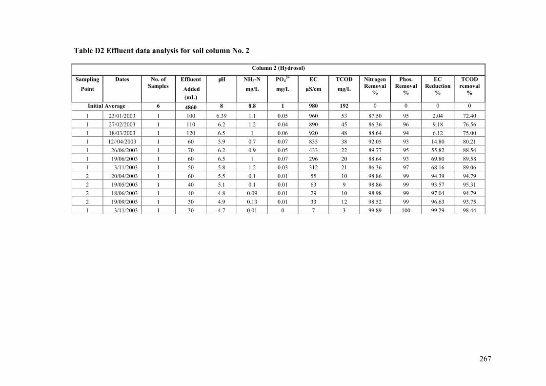
267


Column 2 (Hydrosol)

Sampling Effluent NH3-N PO43+ EC TCOD

Point Added mg/L mg/L µS/cm mg/L

Dates No. of Samples

(mL)

pH

Nitrogen Removal

%

Phos. Removal

%

EC Reduction

%

TCOD removal

%

Initial Average 6 4860 8 8.8 1 980 192 0 0 0 0

1 23/01/2003 1 100 6.39 1.1 0.05 960 53 87.50 95 2.04 72.40 1 27/02/2003 1 110 6.2 1.2 0.04 890 45 86.36 96 9.18 76.56 1 18/03/2003 1 120 6.5 1 0.06 920 48 88.64 94 6.12 75.00 1 12//04/2003 1 60 5.9 0.7 0.07 835 38 92.05 93 14.80 80.21 1 26/06/2003 1 70 6.2 0.9 0.05 433 22 89.77 95 55.82 88.54 1 19/06/2003 1 60 6.5 1 0.07 296 20 88.64 93 69.80 89.58 1 3/11/2003 1 50 5.8 1.2 0.03 312 21 86.36 97 68.16 89.06 2 20/04/2003 1 60 5.5 0.1 0.01 55 10 98.86 99 94.39 94.79 2 19/05/2003 1 40 5.1 0.1 0.01 63 9 98.86 99 93.57 95.31 2 18/06/2003 1 40 4.8 0.09 0.01 29 10 98.98 99 97.04 94.79 2 19/09/2003 1 30 4.9 0.13 0.01 33 12 98.52 99 96.63 93.75 1 3/11/2003 1 30 4.7 0.01 0 7 3 99.89 100 99.29 98.44

268

Table E2 Feeding and collecting effluent for column No. 2 (Hydrosol) from the different sampling points

Acc. First Second Third Fourth Pond. Volume Days Feed Sample Sample Sample Sampling Time Available Wetting Acc.

Days Date Feed mL mL Point Point Point Point mL Evapor.

Effluent Saturate

mL Point Distance mm

0 12/12/2003 0 0 1 12/12/2002 120 120 2 (occurred) 2 13/12/2002 120 240 3 14/12/2002 80 320 10 20/12/2002 120 440 13 22/12/2002 120 560 14 23/12/2002 100 660 18 26/12/2003 100 760 15 (Noticed) 18 150 45 21/01/2003 200 960 100 51 27/01/2003 220 1180 71 15/02/2003 220 1400 88 2/03/2003 180 1580 110

110 23/03/2003 200 1780 120 130 10/04/2003 200 1980 147 25/04/2003 200 2180 60 60 147 450 171 18/05/2003 200 2380 40 172 19/05/2003 160 2540 186 2/06/2003 200 2740 203 18/06/2003 200 2940 40 216 30/06/2003 150 3090 70 229 12/07/2003 150 3240 249 30/07/2003 200 3440 268 18/08/2003 120 3560 269 19/08/2003 100 3660 60 288 7/09/2003 200 3860 300 18/09/2003 200 4060 30 315 30/10/2003 200 4260 316 31/10/2003 200 4460 323 7/11/2003 200 4660 50 30 323 810 337 20/11/2003 200 4860

Total 4860 570 170 50 2750 1320

269


Column 3 (Podosol)


Point added mg/L mg/L µS/cm mg/L


(mL)

pH

Nitrogen Removal

%

Phos. Removal

%

EC Reduction

%

TCOD removal

% Intial average 4 4800 8.00 8.80 1 980 192 0.00 0 0.00 0.00 4 14/12/2002 1 120 4.50 2.00 0.18 445 47.0 77.3 82.0 54.6 75.5 4 16/12/2003 2 240 3.60 0.70 0.62 16.3 53.0 92.0 38.0 98.3 72.4 4 18/12/2003 1 120 3.80 0.60 1.29 134 56.0 93.2 -29.0 86.3 70.8 4 20/12/2003 2 240 3.95 2.80 0.70 1090 68.0 68.2 30.0 -11.2 64.6 3 27/12/2003 1 120 5.75 3.90 42.5 1055 66.0 55.7 -4145 -7.65 65.6 3 28/12/2003 1 120 4.05 2.30 42.5 968 72.0 73.9 -4145 1.22 62.5 3 2/01/2003 1 120 4.24 10.0 44.4 560 91.0 -13.6 -4339 42.9 52.6 3 4/01/2003 1 120 4.08 8.80 10.00 867 82.0 0.00 -900 11.5 57.3 3 6/01/2003 1 120 4.05 7.00 5.75 1007 68.0 20.5 -475 -2.76 64.6 3 10/01/2003 1 120 4.16 7.80 8.56 977 55.0 11.4 -756 0.31 71.4 2 12/01/2003 1 120 4.79 54.0 9.22 478 99.0 -513.6 -822 51.22 48.4 2 14/01/2003 1 120 4.43 22.0 8.83 870 67.0 -150.0 -783 11.2 65.1 2 15/01/2003 1 120 4.48 36.0 7.91 1023 79.0 -309.1 -691 -4.39 58.9 2 16/01/2003 1 120 4.68 38.0 11.2 1002 63.0 -331.8 -1020 -2.24 67.2 2 17/01/2003 1 120 4.87 59.0 13.8 987 109 -570.5 -1281 -0.71 43.2 2 18/01/2003 1 120 4.38 41.0 7.60 942 129 -365.9 -660 3.88 32.8 1 21/01/2003 1 120 5.60 23.0 2.20 870 120 -161.4 -120 11.2 37.5 1 24/01/2003 1 120 5.80 48.0 1.10 760 127 -445.5 -10.0 22.4 33.9 1 29/01/2003 1 120 5.92 43.0 0.90 799 123 -388.6 10.0 18.5 35.9 1 6/02/2003 1 120 6.01 36.0 2.80 840 119 -309.1 -180 14.3 38.0 1 7/02/2003 1 120 5.82 26.0 1.40 855 134 -195.5 -40.0 12.8 30.2 1 8/02/2003 1 120 6.10 49.0 0.89 901 139 -456.8 11.0 8.06 27.6 1 9/02/2003 1 120 5.95 54.0 0.64 870 127 -513.6 36.0 11.2 33.9 1 10/02/2003 1 120 5.50 61.0 1.03 910 135 -593.2 -3.0 7.14 29.7 1 11/02/2003 1 120 5.60 59.0 2.10 896 108 -570.5 -110 8.57 43.8

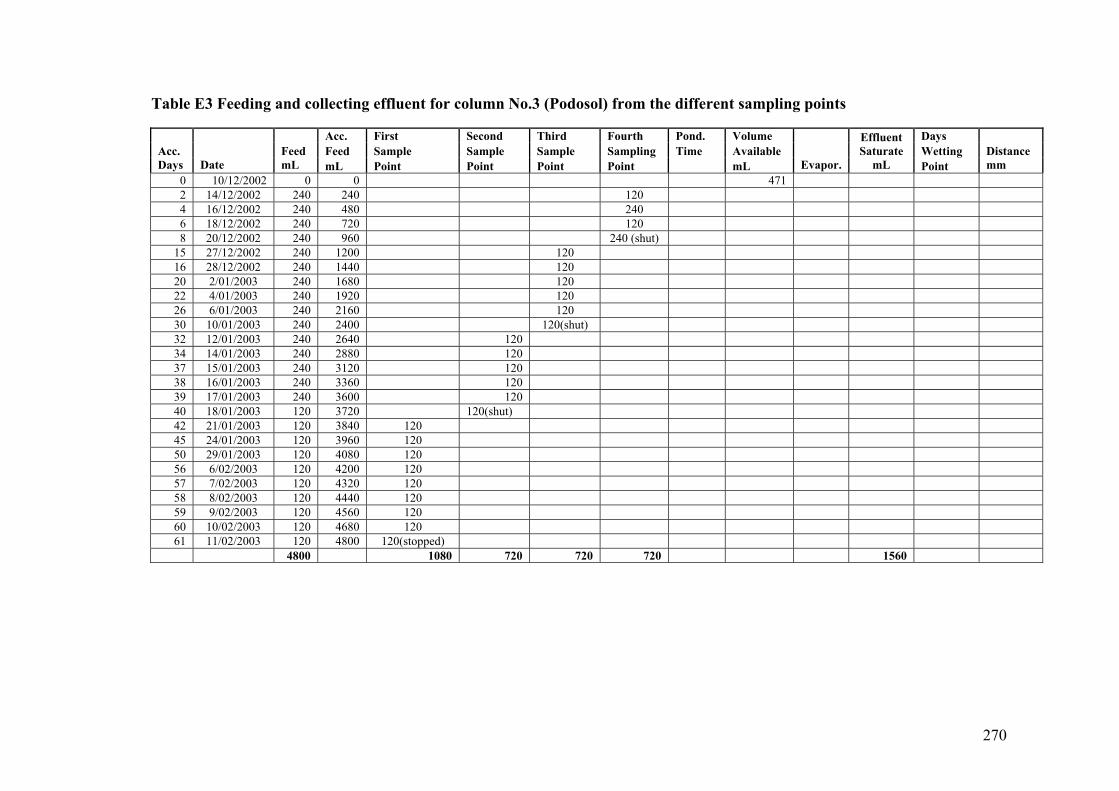
270

Table E3 Feeding and collecting effluent for column No.3 (Podosol) from the different sampling points



Effluent Saturate


0 10/12/2002 0 0 471 2 14/12/2002 240 240 120 4 16/12/2002 240 480 240 6 18/12/2002 240 720 120 8 20/12/2002 240 960 240 (shut)

15 27/12/2002 240 1200 120 16 28/12/2002 240 1440 120 20 2/01/2003 240 1680 120 22 4/01/2003 240 1920 120 26 6/01/2003 240 2160 120 30 10/01/2003 240 2400 120(shut) 32 12/01/2003 240 2640 120 34 14/01/2003 240 2880 120 37 15/01/2003 240 3120 120 38 16/01/2003 240 3360 120 39 17/01/2003 240 3600 120 40 18/01/2003 120 3720 120(shut) 42 21/01/2003 120 3840 120 45 24/01/2003 120 3960 120 50 29/01/2003 120 4080 120 56 6/02/2003 120 4200 120 57 7/02/2003 120 4320 120 58 8/02/2003 120 4440 120 59 9/02/2003 120 4560 120 60 10/02/2003 120 4680 120 61 11/02/2003 120 4800 120(stopped)

4800 1080 720 720 720 1560

271

Table D.4 Feeding and collecting effluent for column No. 4 (Black Sodosol from the different sampling points

Column 4 (Black Sodosol)




(mL)

pH

Nitrogen Removal

%

Phos. Removal

%

EC Reduction

%

TCOD removal

%

Intial average 6 5520 8.00 8.80 1.00 980 192 0.00 0.00 0.00 0.00 1 12/12/2002 1 110 5.60 1.50 0.63 194 54.0 83.0 37.0 80.2 71.9 1 16/12/2002 1 120 6.99 1.10 0.25 727 44.0 87.5 75.0 25.8 77.1 1 23/01/2003 1 100 6.02 0.40 0.23 74.2 43.0 95.5 77.0 92.4 77.6 1 25/02/2003 1 100 6.63 0.45 0.28 38.8 37.0 94.9 72.0 96.0 80.7 1 2/03/2003 1 60 5.80 0.60 0.52 22.9 25.0 93.2 48.0 97.7 87.0 1 20/08/2003 1 80 6.20 0.80 0.30 30.0 22.0 90.9 70.0 96.9 88.5 2 18/11/2003 1 40 5.60 0.10 0.01 12.0 5.0 98.9 99.0 98.8 97.4

272

Table D.5 Feeding and collecting effluent for column No.4 (Black Sodosol) from the different sampling points

Acc. Days

Date Feed mL

Evapor. Distance mm

Acc. Feed mL

First Sample Point

Second Sample Point

Third Sample Point


Pond. Time

Volume Available mL

Effluent Saturate mL

Days Wetting Point

0 0 706.5 1 12/12/2002 120 120 110 3 2 80 2 13/12/2002 240 360 3 15/12/2003 240 600

12 23/12/2002 240 840 120 22 2/01/2003 240 1080 41 21/01/2003 240 1320 75 25/02/2003 500 1820 100

108 28/03/2003 500 2320 100 143 3/05/2003 500 2820 179 10/06/2003 500 3320 60 223 25/07/2003 400 3720 246 18/08/2003 300 4020 247 19/08/2003 300 4320 281 25/09/2003 300 4620 80 304 18/10/2003 300 4920 317 31/10/2003 300 5220 337 20/11/2003 300 5520 40 330 390

Total 5520 460 40 2750 2270.00

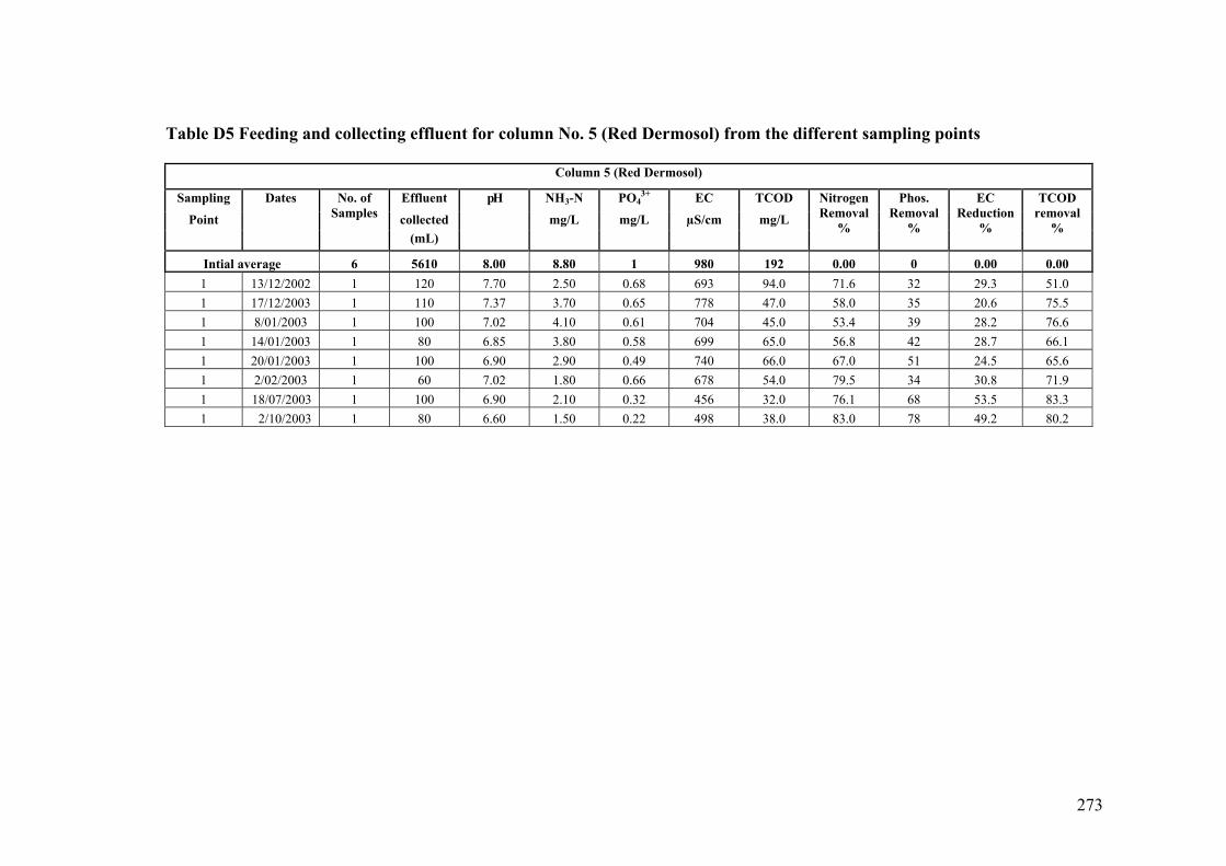
273

Table D5 Feeding and collecting effluent for column No. 5 (Red Dermosol) from the different sampling points

Column 5 (Red Dermosol)


Point collected mg/L mg/L µS/cm mg/L


(mL)

pH

Nitrogen Removal

%

Phos. Removal

%

EC Reduction

%

TCOD removal

%

Intial average 6 5610 8.00 8.80 1 980 192 0.00 0 0.00 0.00 1 13/12/2002 1 120 7.70 2.50 0.68 693 94.0 71.6 32 29.3 51.0 1 17/12/2003 1 110 7.37 3.70 0.65 778 47.0 58.0 35 20.6 75.5 1 8/01/2003 1 100 7.02 4.10 0.61 704 45.0 53.4 39 28.2 76.6 1 14/01/2003 1 80 6.85 3.80 0.58 699 65.0 56.8 42 28.7 66.1 1 20/01/2003 1 100 6.90 2.90 0.49 740 66.0 67.0 51 24.5 65.6 1 2/02/2003 1 60 7.02 1.80 0.66 678 54.0 79.5 34 30.8 71.9 1 18/07/2003 1 100 6.90 2.10 0.32 456 32.0 76.1 68 53.5 83.3 1 2/10/2003 1 80 6.60 1.50 0.22 498 38.0 83.0 78 49.2 80.2

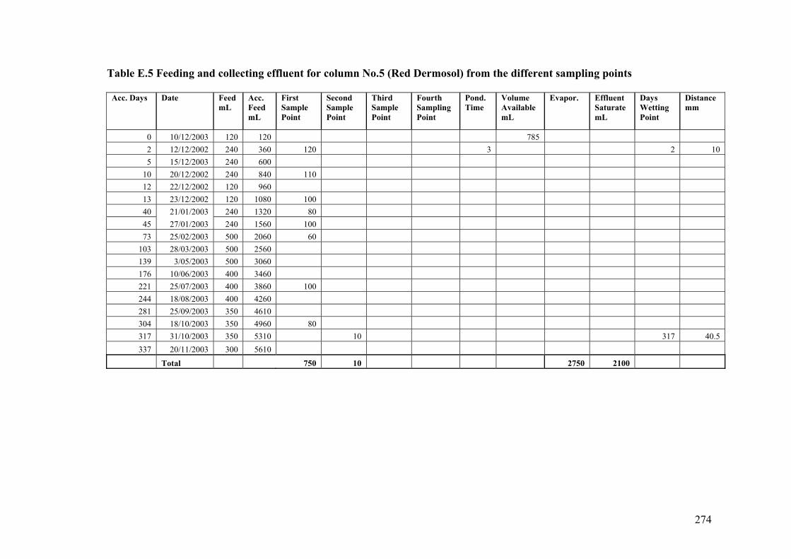
274

Table E.5 Feeding and collecting effluent for column No.5 (Red Dermosol) from the different sampling points

Acc. Days

Date

Feed mL

Acc. Feed mL

First Sample Point

Second Sample Point

Third Sample Point


Pond. Time

Volume Available mL

Evapor.

Effluent Saturate mL

Days Wetting Point

Distance mm

0 10/12/2003 120 120 785 2 12/12/2002 240 360 120 3 2 10 5 15/12/2003 240 600

10 20/12/2002 240 840 110 12 22/12/2002 120 960 13 23/12/2002 120 1080 100 40 21/01/2003 240 1320 80 45 27/01/2003 240 1560 100 73 25/02/2003 500 2060 60

103 28/03/2003 500 2560 139 3/05/2003 500 3060 176 10/06/2003 400 3460 221 25/07/2003 400 3860 100 244 18/08/2003 400 4260 281 25/09/2003 350 4610 304 18/10/2003 350 4960 80 317 31/10/2003 350 5310 10 317 40.5 337 20/11/2003 300 5610

Total 750 10 2750 2100

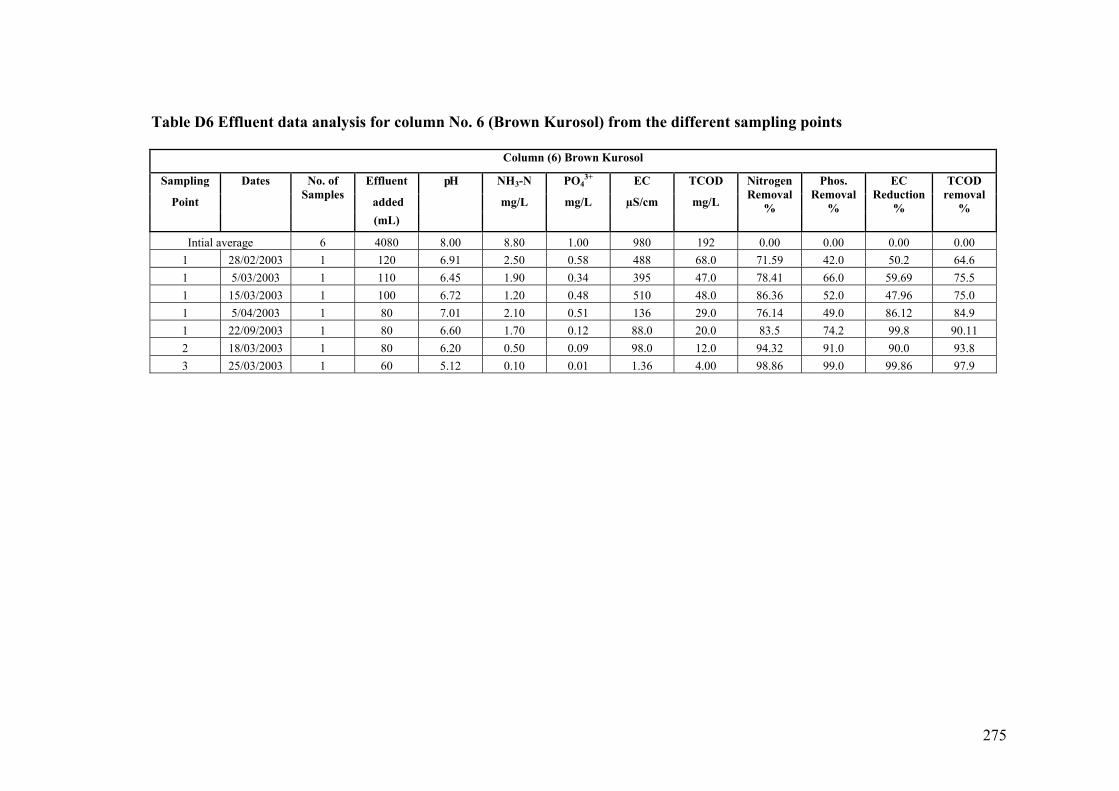
275

Table D6 Effluent data analysis for column No. 6 (Brown Kurosol) from the different sampling points

Column (6) Brown Kurosol




(mL)

pH

Nitrogen Removal

%

Phos. Removal

%

EC Reduction

%

TCOD removal

%

Intial average 6 4080 8.00 8.80 1.00 980 192 0.00 0.00 0.00 0.00 1 28/02/2003 1 120 6.91 2.50 0.58 488 68.0 71.59 42.0 50.2 64.6 1 5/03/2003 1 110 6.45 1.90 0.34 395 47.0 78.41 66.0 59.69 75.5 1 15/03/2003 1 100 6.72 1.20 0.48 510 48.0 86.36 52.0 47.96 75.0 1 5/04/2003 1 80 7.01 2.10 0.51 136 29.0 76.14 49.0 86.12 84.9 1 22/09/2003 1 80 6.60 1.70 0.12 88.0 20.0 83.5 74.2 99.8 90.11 2 18/03/2003 1 80 6.20 0.50 0.09 98.0 12.0 94.32 91.0 90.0 93.8 3 25/03/2003 1 60 5.12 0.10 0.01 1.36 4.00 98.86 99.0 99.86 97.9

276

Table E6 Feeding and collecting effluent for column No.6 (Brown Kurosol) from the different sampling points



Effluent Saturate


0 10/12/2002 120 120 314 2 12/12/2002 120 240 2 2 130

10 20/12/2002 240 480 12 22/12/2002 240 720 13 23/12/2002 240 960 41 21/01/2003 240 1200 47 27/01/2003 240 1440 75 25/02/2003 240 1680 120

101 21/03/2003 240 1920 110 80 101 430 141 3/05/2003 240 2160 100 178 10/06/2003 240 2400 80 199 1/07/2003 240 2640 60 199 800 238 10/08/2003 240 2880 247 19/08/2003 240 3120 265 7/09/2003 240 3360 306 18/10/2003 240 3600 80 325 7/11/2003 240 3840 338 20/11/2003 240 4080

490 80 60 2750 700

277

Table D7 Effluent data analysis for column No. 7 (Brown Vertosol) from the different sampling points

Column 7 (Brown Vertosol) Sampling Effluent NH3-N PO4

3+ EC TCOD



(mL)

pHw

Nitrogen Removal

%

Phos. Removal

%

EC Reduction

%

TCOD removal

%

Initial average 6 6080 8.00 8.80 1.00 980 192.0 0.00 0.00 0.00 0.00 1 12/12/2002 1 120 7.33 2.20 0.08 395 6.00 75.0 92.0 59.7 96.9 1 13/12/2002 1 120 6.92 2.20 0.08 439 8.00 75.0 92.0 55.2 95.8 1 7/01/2003 1 120 7.02 1.90 0.07 382 12.0 78.4 93.0 61.0 93.8 1 20/01/2003 1 120 7.01 1.80 0.10 312 34.0 79.5 90.0 68.2 82.3 1 28/01/2003 1 120 6.80 2.10 0.30 284 24.0 76.1 70.0 71.0 87.5 1 22/02/2003 1 100 6.80 2.20 0.30 388 22.0 75.0 70.0 60.4 88.5 1 5/03/2003 1 110 6.50 2.01 0.50 411 16.0 77.2 50.0 58.1 91.7 1 4/05/2003 1 120 6.60 1.10 0.30 311 19.0 87.5 70.0 68.3 90.1 2 28/03/2003 1 60 5.50 1.00 0.20 332 17.0 88.6 80.0 66.1 91.1 2 25/04/2003 1 100 5.90 0.70 0.11 121 2.00 92.0 89.0 87.7 99.0 2 1/07/2003 1 80 6.01 1.00 0.40 150 10.0 88.6 60.0 84.7 94.8 2 15/09/2003 1 60 5.80 1.30 0.32 110 15.0 85.2 68.0 88.8 92.2 3 25/04/2003 1 30 4.50 0.01 0.10 4.36 1.00 99.9 90.0 99.6 99.5 3 31/10/2003 1 40 5.10 0.02 0.08 26.0 6.00 99.8 92.0 97.3 96.9

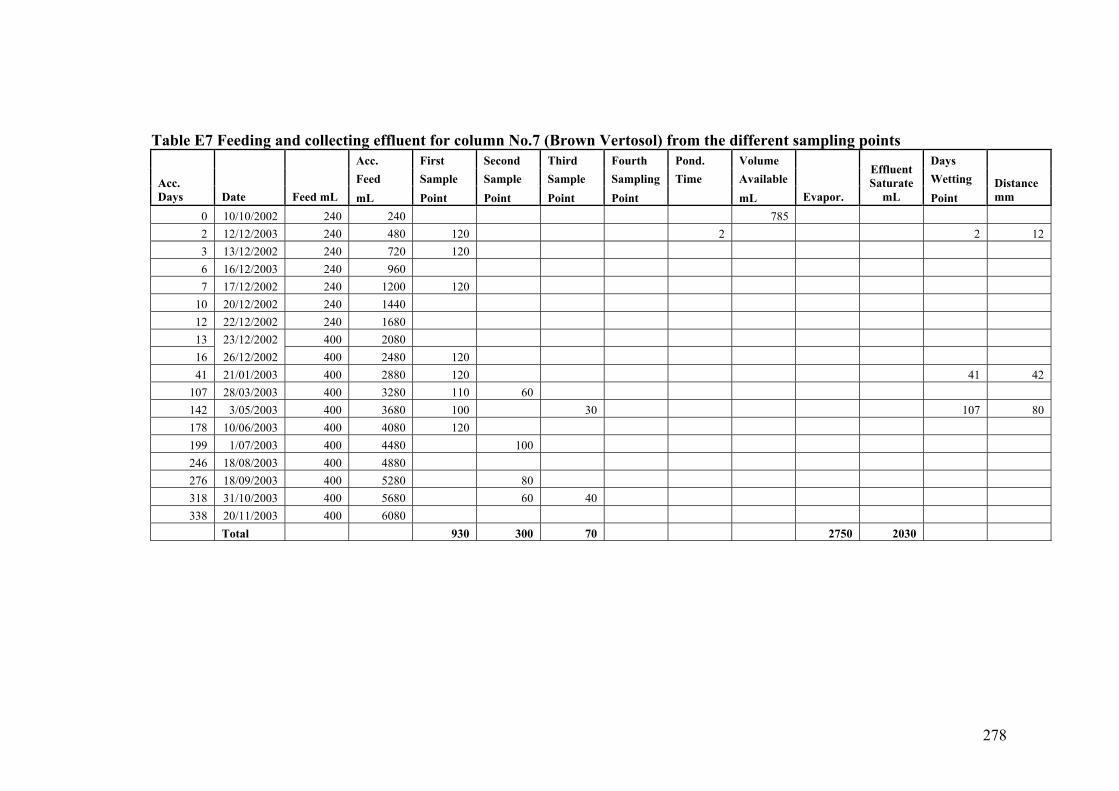
278

Table E7 Feeding and collecting effluent for column No.7 (Brown Vertosol) from the different sampling points



Effluent Saturate


0 10/10/2002 240 240 785 2 12/12/2003 240 480 120 2 2 12 3 13/12/2002 240 720 120 6 16/12/2003 240 960 7 17/12/2002 240 1200 120

10 20/12/2002 240 1440 12 22/12/2002 240 1680 13 23/12/2002 400 2080 16 26/12/2002 400 2480 120 41 21/01/2003 400 2880 120 41 42

107 28/03/2003 400 3280 110 60 142 3/05/2003 400 3680 100 30 107 80 178 10/06/2003 400 4080 120 199 1/07/2003 400 4480 100 246 18/08/2003 400 4880 276 18/09/2003 400 5280 80 318 31/10/2003 400 5680 60 40 338 20/11/2003 400 6080

Total 930 300 70 2750 2030

279

Table D8 Feeding and collecting effluent for column No. 8 (Dermosol) from the different sampling points

Column 8 Dermosol




(mL)

pH

Nitrogen Removal

%

Phos. Removal

%

EC Reduction

%

TCOD removal

%

Intial average 6 7020 8 8.8 1 980 192 0.00 0.00 0.00 0.00 1 12/12/2002 1 120 6.41 1.5 0.08 24 8 82.95 92 97.55 95.83 1 18/12/2002 1 120 6.22 2.2 0.08 126 11 75.00 92 87.14 94.27 1 20/01/2003 1 100 6.72 1.1 0.09 98 12 87.50 91 90.00 93.75 1 13/02/2003 1 100 6.8 1.9 0.1 87 18 78.41 90 91.12 90.63 1 5/03/2003 1 110 6.5 1.3 0.15 168 6 85.23 85 82.86 96.88 1 1/06/2003 1 120 6.2 2.1 0.21 320 10 76.14 79 67.35 94.79 1 2/08/2003 1 120 6.7 1.8 0.08 168 15 79.55 92 82.86 92.19 1 10/09/2003 1 120 7.01 1.9 0.2 110 22 78.41 80 88.78 88.54 1 18/10/2003 1 120 6.8 1.3 0.11 132 16 85.23 89 86.53 91.67 2 20/04/2003 1 40 5.72 0.5 0.01 36 7 94.32 99 96.33 96.35 2 10/06/2003 1 120 5.32 1.1 0.09 88 13 87.50 91 91.02 93.23 2 20/07/2003 1 120 5.18 0.9 0.01 100 6 89.77 99 89.80 96.88 2 2/10/2003 1 120 5.34 0.7 0.02 54 10 92.05 98 94.49 94.79 2 18/11/2003 1 60 4.9 1.1 0.01 23 8 87.50 99 97.65 95.83 3 18/11/2003 1 60 5.1 0.4 0.01 20 5 95.45 99 97.96 97.40

280

Table E8 Feeding and collecting effluent for column No.8 (Dermosol) from the different sampling points



Effluent Saturate


0 10/12/2002 120 120 1020.5 1 11/12/2002 240 360 120 2 80 2 12/12/2002 240 600 120 3 3 13/12/2003 240 840 7 17/12/2002 240 1080

23 2/01/2003 240 1320 100 36 15/01/2003 500 1820 100 46 25/01/2003 500 2320 79 28/02/2003 500 2820 110

114 3/04/2003 500 3320 40 114 380 147 7/05/2003 500 3820 180 10/06/2003 400 4220 120 120 224 25/07/2003 400 4620 120 247 18/08/2003 400 5020 120 248 19/08/2003 400 5420 282 25/09/2003 400 5820 120 305 18/10/2003 400 6220 120 318 31/10/2003 400 6620 120 338 20/11/2003 400 7020 60 60 330 840

Total 7020 1030 460 60 2750 2720

281

Table D9 Effluent data analysis for soil column No.9 (Yellow Dermosol)

Column 9 (Yellow Dermosol)




(mL)

pH

Nitrogen Removal

%

Phos. Removal

%

EC Reduction

%

TCOD removal

%

Intial average 6 6360 8.00 8.80 1.00 980 192 0.00 0.00 0.00 0.00 1 11/12/2002 1 120 6.89 3.70 0.08 508 47.0 58.0 92.0 48.2 75.5 1 12/12/2002 2 240 6.92 4.80 0.08 467 53.0 45.5 92.0 52.3 72.4 1 12/01/2003 1 120 7.00 1.00 0.08 572 58.0 88.6 92.0 41.6 69.8 1 17/01/2003 1 120 6.94 1.90 0.09 482 49.0 78.4 91.0 50.8 74.5 1 22/01/2003 1 120 6.89 1.80 0.12 522 42.0 79.5 88.0 46.7 78.1 1 25/02/2003 1 120 6.80 1.90 0.09 466 51.0 78.4 91.0 52.4 73.4 1 6/05/2003 2 240 6.50 2.10 0.38 365 42.0 76.1 62.0 62.8 78.1 1 25/08/2003 1 120 6.80 1.30 0.22 387 38.0 85.2 78.0 60.5 80.2 2 4/03/2003 1 40 6.30 0.60 0.01 288 12.0 93.2 99.0 70.6 93.8 2 30/03/2003 1 80 5.90 0.30 0.01 150 10.0 96.6 99.0 84.7 94.8 2 30/06/2003 1 60 6.20 0.40 0.01 126 15.0 95.5 99.0 87.1 92.2 2 19/08/2003 1 100 5.70 0.60 0.02 160 8.0 93.2 98.0 83.7 95.8 2 15/09/2003 1 100 6.00 0.70 0.03 110 17.0 92.0 97.0 88.8 91.1

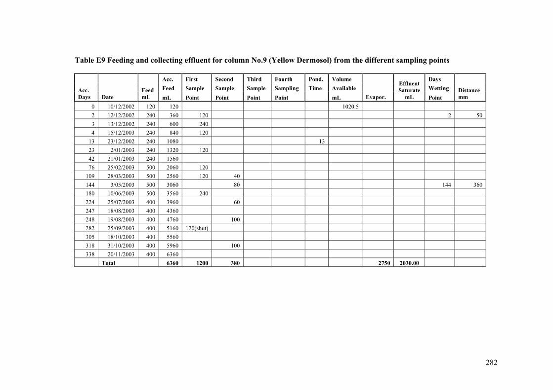
282

Table E9 Feeding and collecting effluent for column No.9 (Yellow Dermosol) from the different sampling points



Effluent Saturate


0 10/12/2002 120 120 1020.5 2 12/12/2002 240 360 120 2 50 3 13/12/2002 240 600 240 4 15/12/2003 240 840 120

13 23/12/2002 240 1080 13 23 2/01/2003 240 1320 120 42 21/01/2003 240 1560 76 25/02/2003 500 2060 120

109 28/03/2003 500 2560 120 40 144 3/05/2003 500 3060 80 144 360 180 10/06/2003 500 3560 240 224 25/07/2003 400 3960 60 247 18/08/2003 400 4360 248 19/08/2003 400 4760 100 282 25/09/2003 400 5160 120(shut) 305 18/10/2003 400 5560 318 31/10/2003 400 5960 100 338 20/11/2003 400 6360

Total 6360 1200 380 2750 2030.00

283

Table D10 Effluent data analysis for the soil column No.10 (Yellow Chromosol) Column 10 (Yellow Chromosol)


Point collected mg/L mg/L µS/cm mg/L


(mL)

pH

Nitrogen Removal

%

Phos. Removal

%

EC Reduction

%

TCOD removal

%

Initial average 6 6360 8.00 8.80 1.00 980 192 0.00 0.00 0.00 0.00 1 12/12/2002 1 120 7.12 5.70 0.78 674 54.0 35.2 22.0 31.2 71.9 1 12/12/2002 2 240 7.10 5.20 0.58 498 74.0 40.9 42.0 49.2 61.5 1 7/01/2003 1 100 7.20 4.20 0.54 572 88.0 52.3 46.0 41.6 54.2 1 20/01/2003 1 120 7.02 2.30 0.58 486 72.0 73.9 42.0 50.4 62.5 1 5/02/2003 1 100 6.99 1.80 0.68 488 66.0 79.5 32.0 50.2 65.6 1 25/02/2003 1 110 6.80 2.90 0.88 567 45.0 67.0 12.0 42.1 76.6 1 20/05/2003 1 120 7.12 3.00 0.70 399 40.0 65.9 30.0 59.3 79.2 1 1/08/2003 1 120 6.88 2.20 0.60 522 45.0 75.0 40.0 46.7 76.6 2 7/03/2003 1 80 6.10 1.10 0.09 320 20.0 87.5 91.0 67.3 89.6 2 20/03/2003 1 80 5.80 0.90 0.08 288 18.0 89.8 92.0 70.6 90.6 2 3/05/2003 1 60 6.20 0.80 0.09 270 22.0 90.9 91.0 72.4 88.5 2 25/07/2003 1 100 6.50 0.50 0.09 310 16.0 94.3 91.0 68.4 91.7 2 22/08/2003 1 100 6.30 2.00 0.08 289 12.0 77.3 92.0 70.5 93.8 3 20/04/2003 1 40 5.70 0.09 0.01 74.0 4.00 99.0 99.0 92.4 97.9 3 12/11/2003 1 40 5.50 0.02 0.03 100 8.00 99.8 97.0 89.8 95.8

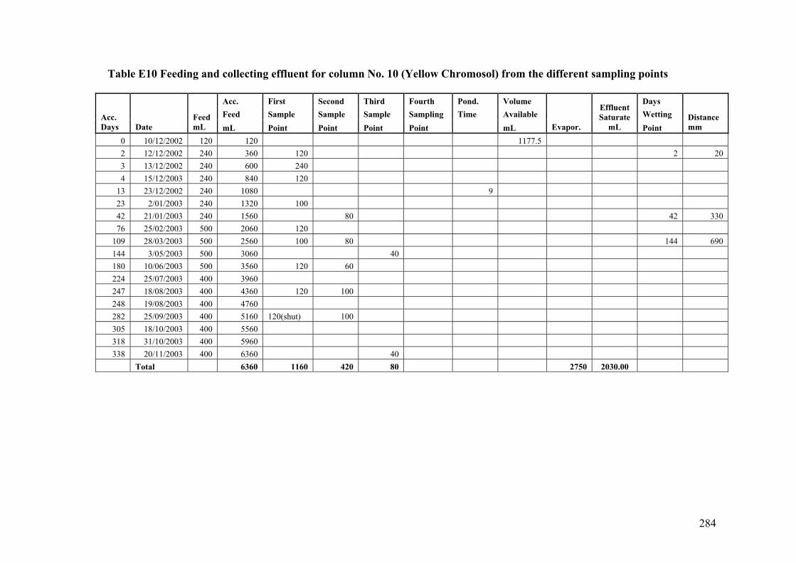
284

Table E10 Feeding and collecting effluent for column No. 10 (Yellow Chromosol) from the different sampling points



Effluent Saturate


0 10/12/2002 120 120 1177.5 2 12/12/2002 240 360 120 2 20 3 13/12/2002 240 600 240 4 15/12/2003 240 840 120

13 23/12/2002 240 1080 9 23 2/01/2003 240 1320 100 42 21/01/2003 240 1560 80 42 330 76 25/02/2003 500 2060 120

109 28/03/2003 500 2560 100 80 144 690 144 3/05/2003 500 3060 40 180 10/06/2003 500 3560 120 60 224 25/07/2003 400 3960 247 18/08/2003 400 4360 120 100 248 19/08/2003 400 4760 282 25/09/2003 400 5160 120(shut) 100 305 18/10/2003 400 5560 318 31/10/2003 400 5960 338 20/11/2003 400 6360 40

Total 6360 1160 420 80 2750 2030.00

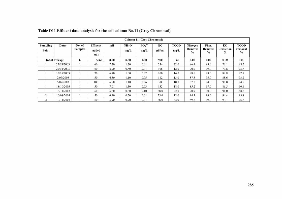
285

Table D11 Effluent data analysis for the soil column No.11 (Grey Chromosol)

Column 11 (Grey Chromosol)




(mL)

pH

Nitrogen Removal

%

Phos. Removal

%

EC Reduction

%

TCOD removal

%

Intial average 6 5660 8.00 8.80 1.00 980 192 0.00 0.00 0.00 0.00 1 25/03/2003 1 60 7.20 1.20 0.01 234 22.0 86.4 99.0 76.1 88.5 1 20/04/2003 1 60 6.90 0.80 0.01 198 12.0 90.9 99.0 79.8 93.8 1 10/05/2003 1 70 6.70 1.00 0.02 100 14.0 88.6 98.0 89.8 92.7 1 2/07/2003 1 50 6.50 1.10 0.05 112 13.0 87.5 95.0 88.6 93.2 1 5/09/2003 1 100 6.80 1.10 0.06 98 10.0 87.5 94.0 90.0 94.8 1 18/10/2003 1 50 7.01 1.30 0.03 132 18.0 85.2 97.0 86.5 90.6 1 18/11/2003 1 60 6.60 0.80 0.10 88.0 22.0 90.9 90.0 91.0 88.5 2 10/08/2003 1 50 6.10 0.50 0.01 55.0 12.0 94.3 99.0 94.4 93.8 2 10/11/2003 1 50 5.90 0.90 0.01 68.0 8.00 89.8 99.0 93.1 95.8

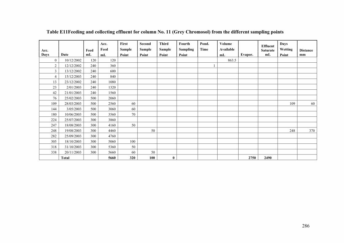
286

Table E11Feeding and collecting effluent for column No. 11 (Grey Chromosol) from the different sampling points



Effluent Saturate


0 10/12/2002 120 120 863.5 2 12/12/2002 240 360 1 3 13/12/2002 240 600 4 15/12/2003 240 840

13 23/12/2002 240 1080 23 2/01/2003 240 1320 42 21/01/2003 240 1560 76 25/02/2003 500 2060

109 28/03/2003 500 2560 60 109 60 144 3/05/2003 500 3060 60 180 10/06/2003 500 3560 70 224 25/07/2003 300 3860 247 18/08/2003 300 4160 50 248 19/08/2003 300 4460 50 248 370 282 25/09/2003 300 4760 305 18/10/2003 300 5060 100 318 31/10/2003 300 5360 50 338 20/11/2003 300 5660 60 50

Total 5660 320 100 0 2750 2490

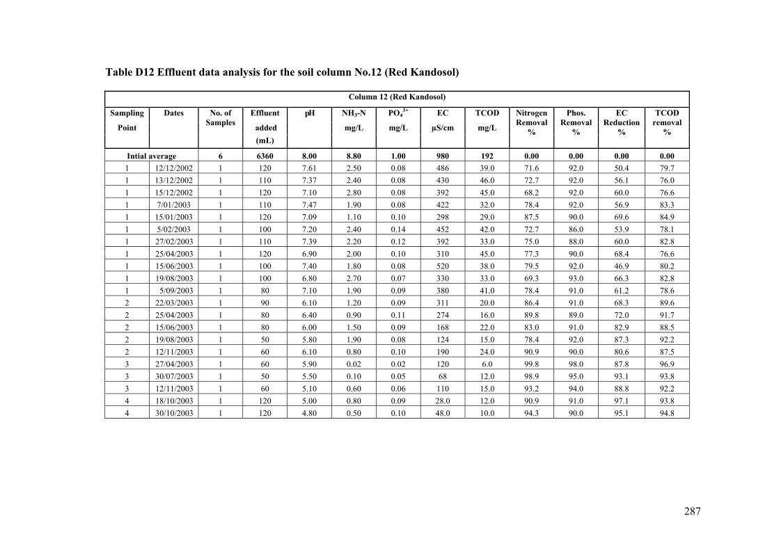
287

Table D12 Effluent data analysis for the soil column No.12 (Red Kandosol)

Column 12 (Red Kandosol)




(mL)

pH

Nitrogen Removal

%

Phos. Removal

%

EC Reduction

%

TCOD removal

%

Intial average 6 6360 8.00 8.80 1.00 980 192 0.00 0.00 0.00 0.00 1 12/12/2002 1 120 7.61 2.50 0.08 486 39.0 71.6 92.0 50.4 79.7 1 13/12/2002 1 110 7.37 2.40 0.08 430 46.0 72.7 92.0 56.1 76.0 1 15/12/2002 1 120 7.10 2.80 0.08 392 45.0 68.2 92.0 60.0 76.6 1 7/01/2003 1 110 7.47 1.90 0.08 422 32.0 78.4 92.0 56.9 83.3 1 15/01/2003 1 120 7.09 1.10 0.10 298 29.0 87.5 90.0 69.6 84.9 1 5/02/2003 1 100 7.20 2.40 0.14 452 42.0 72.7 86.0 53.9 78.1 1 27/02/2003 1 110 7.39 2.20 0.12 392 33.0 75.0 88.0 60.0 82.8 1 25/04/2003 1 120 6.90 2.00 0.10 310 45.0 77.3 90.0 68.4 76.6 1 15/06/2003 1 100 7.40 1.80 0.08 520 38.0 79.5 92.0 46.9 80.2 1 19/08/2003 1 100 6.80 2.70 0.07 330 33.0 69.3 93.0 66.3 82.8 1 5/09/2003 1 80 7.10 1.90 0.09 380 41.0 78.4 91.0 61.2 78.6 2 22/03/2003 1 90 6.10 1.20 0.09 311 20.0 86.4 91.0 68.3 89.6 2 25/04/2003 1 80 6.40 0.90 0.11 274 16.0 89.8 89.0 72.0 91.7 2 15/06/2003 1 80 6.00 1.50 0.09 168 22.0 83.0 91.0 82.9 88.5 2 19/08/2003 1 50 5.80 1.90 0.08 124 15.0 78.4 92.0 87.3 92.2 2 12/11/2003 1 60 6.10 0.80 0.10 190 24.0 90.9 90.0 80.6 87.5 3 27/04/2003 1 60 5.90 0.02 0.02 120 6.0 99.8 98.0 87.8 96.9 3 30/07/2003 1 50 5.50 0.10 0.05 68 12.0 98.9 95.0 93.1 93.8 3 12/11/2003 1 60 5.10 0.60 0.06 110 15.0 93.2 94.0 88.8 92.2 4 18/10/2003 1 120 5.00 0.80 0.09 28.0 12.0 90.9 91.0 97.1 93.8 4 30/10/2003 1 120 4.80 0.50 0.10 48.0 10.0 94.3 90.0 95.1 94.8

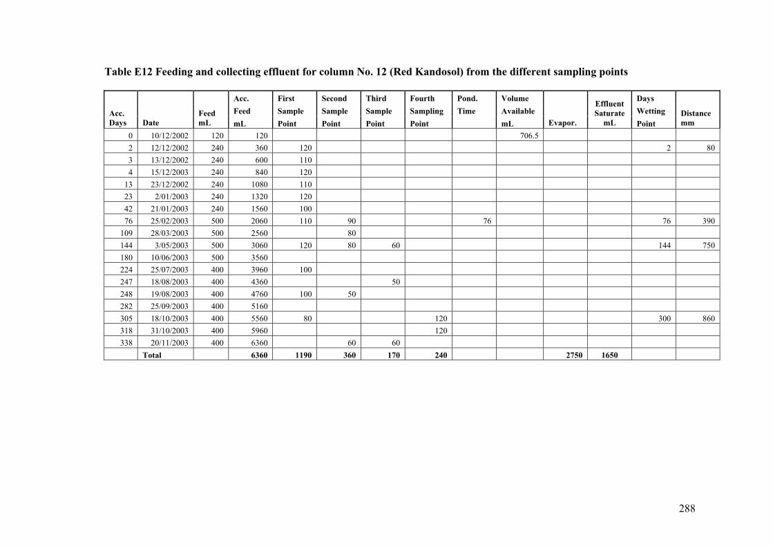
288

Table E12 Feeding and collecting effluent for column No. 12 (Red Kandosol) from the different sampling points



Effluent Saturate


0 10/12/2002 120 120 706.5 2 12/12/2002 240 360 120 2 80 3 13/12/2002 240 600 110 4 15/12/2003 240 840 120

13 23/12/2002 240 1080 110 23 2/01/2003 240 1320 120 42 21/01/2003 240 1560 100 76 25/02/2003 500 2060 110 90 76 76 390

109 28/03/2003 500 2560 80 144 3/05/2003 500 3060 120 80 60 144 750 180 10/06/2003 500 3560 224 25/07/2003 400 3960 100 247 18/08/2003 400 4360 50 248 19/08/2003 400 4760 100 50 282 25/09/2003 400 5160 305 18/10/2003 400 5560 80 120 300 860 318 31/10/2003 400 5960 120 338 20/11/2003 400 6360 60 60

Total 6360 1190 360 170 240 2750 1650

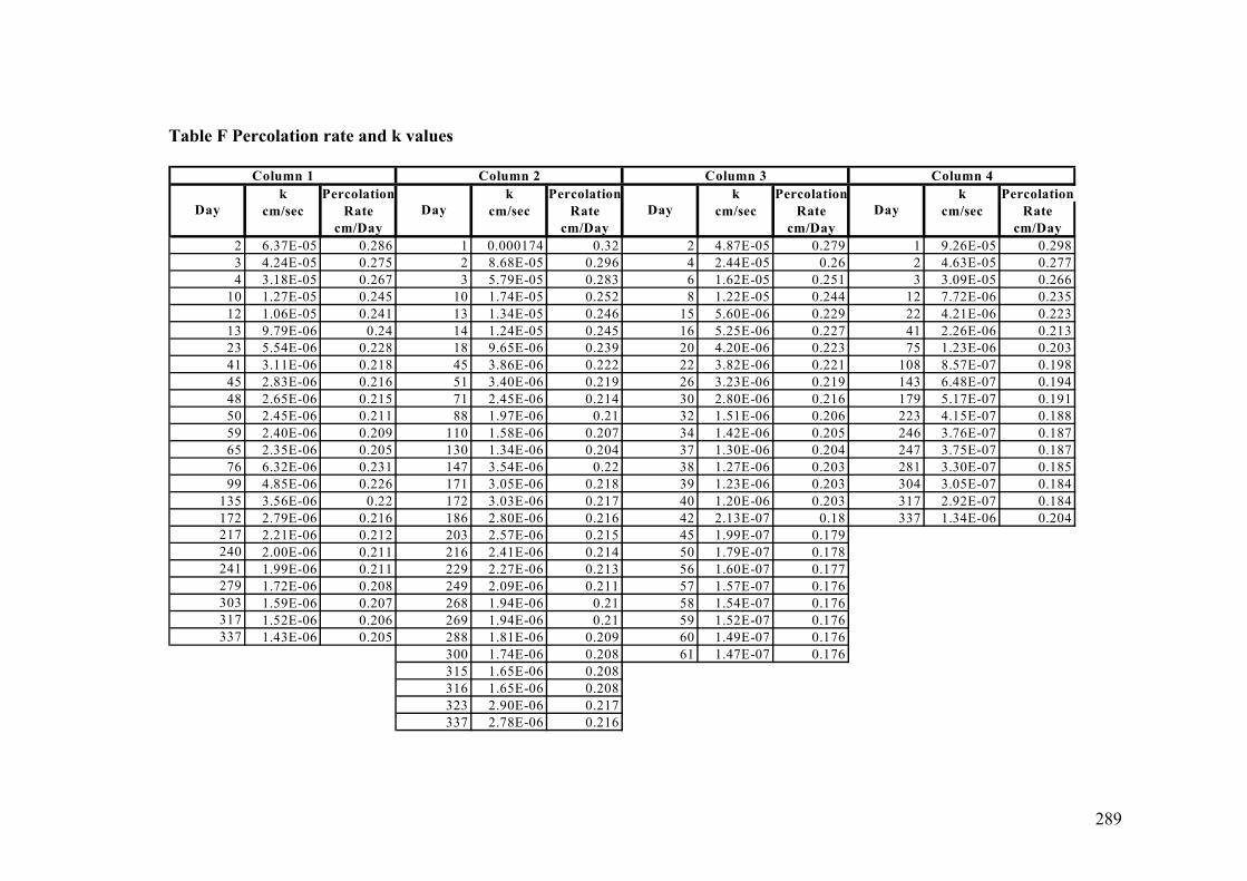
289

Table F Percolation rate and k values

k Percolation k Percolation k Percolation k Percolationcm/sec Rate cm/sec Rate cm/sec Rate cm/sec Rate

cm/Day cm/Day cm/Day cm/Day2 6.37E-05 0.286 1 0.000174 0.32 2 4.87E-05 0.279 1 9.26E-05 0.2983 4.24E-05 0.275 2 8.68E-05 0.296 4 2.44E-05 0.26 2 4.63E-05 0.2774 3.18E-05 0.267 3 5.79E-05 0.283 6 1.62E-05 0.251 3 3.09E-05 0.266

10 1.27E-05 0.245 10 1.74E-05 0.252 8 1.22E-05 0.244 12 7.72E-06 0.23512 1.06E-05 0.241 13 1.34E-05 0.246 15 5.60E-06 0.229 22 4.21E-06 0.22313 9.79E-06 0.24 14 1.24E-05 0.245 16 5.25E-06 0.227 41 2.26E-06 0.21323 5.54E-06 0.228 18 9.65E-06 0.239 20 4.20E-06 0.223 75 1.23E-06 0.20341 3.11E-06 0.218 45 3.86E-06 0.222 22 3.82E-06 0.221 108 8.57E-07 0.19845 2.83E-06 0.216 51 3.40E-06 0.219 26 3.23E-06 0.219 143 6.48E-07 0.19448 2.65E-06 0.215 71 2.45E-06 0.214 30 2.80E-06 0.216 179 5.17E-07 0.19150 2.45E-06 0.211 88 1.97E-06 0.21 32 1.51E-06 0.206 223 4.15E-07 0.18859 2.40E-06 0.209 110 1.58E-06 0.207 34 1.42E-06 0.205 246 3.76E-07 0.18765 2.35E-06 0.205 130 1.34E-06 0.204 37 1.30E-06 0.204 247 3.75E-07 0.18776 6.32E-06 0.231 147 3.54E-06 0.22 38 1.27E-06 0.203 281 3.30E-07 0.18599 4.85E-06 0.226 171 3.05E-06 0.218 39 1.23E-06 0.203 304 3.05E-07 0.184

135 3.56E-06 0.22 172 3.03E-06 0.217 40 1.20E-06 0.203 317 2.92E-07 0.184172 2.79E-06 0.216 186 2.80E-06 0.216 42 2.13E-07 0.18 337 1.34E-06 0.204217 2.21E-06 0.212 203 2.57E-06 0.215 45 1.99E-07 0.179240 2.00E-06 0.211 216 2.41E-06 0.214 50 1.79E-07 0.178241 1.99E-06 0.211 229 2.27E-06 0.213 56 1.60E-07 0.177279 1.72E-06 0.208 249 2.09E-06 0.211 57 1.57E-07 0.176303 1.59E-06 0.207 268 1.94E-06 0.21 58 1.54E-07 0.176317 1.52E-06 0.206 269 1.94E-06 0.21 59 1.52E-07 0.176337 1.43E-06 0.205 288 1.81E-06 0.209 60 1.49E-07 0.176

300 1.74E-06 0.208 61 1.47E-07 0.176315 1.65E-06 0.208316 1.65E-06 0.208323 2.90E-06 0.217337 2.78E-06 0.216

Day Day Day Day

Column 1 Column 2 Column 3 Column 4

290

Table F (Continued) Percolation rate and k values


Day k cm/sec

PercolationRate cm/Day

Day k cm/sec


Day k cm/sec


Day k cm/sec

Percolation Rate cm/Day

2 5.79E-05 0.283 2 7.52E-05 0.291 2 6.94E-05 0.289 1 9.26E-05 0.298 5 2.31E-05 0.259 10 1.5E-05 0.249 3 4.63E-05 0.277 2 4.63E-05 0.277 10 1.16E-05 0.243 12 1.25E-05 0.245 6 2.31E-05 0.259 3 3.09E-05 0.266 12 9.65E-06 0.239 13 1.16E-05 0.243 7 1.98E-05 0.255 7 1.32E-05 0.246 13 8.9E-06 0.238 41 3.67E-06 0.221 10 1.39E-05 0.247 23 4.03E-06 0.222 40 2.89E-06 0.217 47 3.2E-06 0.218 12 1.16E-05 0.243 36 2.57E-06 0.215 45 2.57E-06 0.215 75 2.01E-06 0.211 13 1.07E-05 0.241 46 2.01E-06 0.211 73 1.59E-06 0.207 101 4.93E-06 0.226 16 8.68E-06 0.237 79 1.17E-06 0.202 103 1.12E-06 0.202 141 3.53E-06 0.220 41 1.19E-05 0.244 114 3.86E-06 0.222 139 8.33E-07 0.197 178 2.8E-06 0.216 107 4.54E-06 0.225 147 2.99E-06 0.217 176 6.58E-07 0.194 199 4.65E-06 0.225 142 6.52E-06 0.231 180 2.44E-06 0.214 221 5.24E-07 0.191 238 3.89E-06 0.222 178 5.2E-06 0.227 224 1.96E-06 0.210 244 4.74E-07 0.190 247 3.75E-06 0.221 199 4.65E-06 0.225 247 1.78E-06 0.209 281 4.12E-07 0.188 265 3.49E-06 0.220 246 3.76E-06 0.221 248 1.77E-06 0.209 304 3.81E-07 0.187 306 3.03E-06 0.217 276 3.35E-06 0.219 282 1.56E-06 0.207 317 1.48E-06 0.206 325 2.85E-06 0.216 318 2.91E-06 0.217 305 1.44E-06 0.205 337 1.39E-06 0.205 338 2.74E-06 0.216 338 2.74E-06 0.216 318 1.38E-06 0.205 338 2.88E-06 0.217

291

Table F (Continued) Percolation rate and k values


Day k cm/sec


Day k cm/sec


Day k cm/sec


Day k cm/sec

Percolation Rate cm/Day

2 2.89E-05 0.265 2 1.16E-05 0.243 2 3.47E-05 0.269 2 4.63E-05 0.277 3 1.93E-05 0.255 3 7.72E-06 0.235 3 2.31E-05 0.259 3 3.09E-05 0.266 4 1.45E-05 0.248 4 5.79E-06 0.229 4 1.74E-05 0.252 4 2.31E-05 0.259 13 4.45E-06 0.224 13 1.78E-06 0.209 13 5.34E-06 0.228 13 7.12E-06 0.233 23 2.52E-06 0.214 23 1.01E-06 0.200 23 3.02E-06 0.217 23 4.03E-06 0.222 42 1.38E-06 0.205 42 9.09E-06 0.238 42 1.65E-06 0.208 42 2.2E-06 0.212 76 7.61E-07 0.196 76 5.03E-06 0.226 76 9.14E-07 0.199 76 5.94E-06 0.230 109 5.31E-07 0.191 109 7.33E-06 0.234 109 6.37E-07 0.194 109 4.14E-06 0.223 144 2.89E-06 0.217 144 5.55E-06 0.228 144 4.82E-07 0.190 144 6.03E-06 0.230 180 2.31E-06 0.213 180 4.44E-06 0.224 180 3.86E-07 0.187 180 4.82E-06 0.226 224 1.86E-06 0.209 224 3.57E-06 0.220 224 3.1E-07 0.184 224 3.88E-06 0.222 247 1.69E-06 0.208 247 3.23E-06 0.219 247 2.81E-07 0.183 247 3.51E-06 0.220 248 1.68E-06 0.208 248 3.22E-06 0.219 248 1.73E-06 0.208 248 3.5E-06 0.220 282 1.48E-06 0.206 282 2.83E-06 0.216 282 1.52E-06 0.206 282 3.08E-06 0.218 305 1.37E-06 0.205 305 2.62E-06 0.215 305 1.4E-06 0.205 305 3.26E-06 0.219 318 1.31E-06 0.204 318 2.51E-06 0.214 318 1.35E-06 0.204 318 3.13E-06 0.218 338 1.23E-06 0.203 338 2.36E-06 0.213 338 1.27E-06 0.203 338 2.94E-06 0.217

292

Appendix C

Checklists for Field Sampling

293

Checklist A Site Selection Information

Date / /

Site No.

Priority Level:

Factor Description

Slope

Vegetation

Soil Type

Soil Profile

Land Size

Land Use

Distance From Creeks

Distance from Previous

Site

General Comments

294

Checklist B Field site sampling information

Date: / / 2001

Site No./

GPS Coordinates/ …………N:………………………………E:…………………

Address/

UBD Reference/

Label/

No. Of Samples/

Site Field Description/

Planning Risk Level (priority)/

1) Very High 2) High 3) Medium-High 4) Low 5) Sewered

Expected Soil/

Actual Soil/

Vegetation (Type, assessment and land use)/

Water Sources/

Site Description (Landscape, Structure and use)/

Field Soil Moisture Content/

pH/

Weather Condition/

Ground Condition/

Drainage (creeks and patterns)/

General Comments/

integrated land capability for ecological sustainability of on-site … · 2010-06-09 · wael r....

Documents