integrated genomic circuits - cshlpress.com · 370 chapter 11 | integrated genomic circuits i n...
TRANSCRIPT

CH
AP
TER
11
Integrated Genomic Circuits
11.1 Natural Gene CircuitsDiscover how genes can form toggle switches.
Understand how computer models of genomic circuits can lead to discoveries about learning.
Read genomic circuit diagrams to understand cancer.
Evaluate the influence of genome organization on the whole system.
11.2 Synthetic BiologyUtilize design principles to construct synthetic toggle switches.
Apply engineering principles to measure our understanding of genomes.
Integrate stochastic behavior of proteins and gene regulation.
CAMPMC11_0805382194.QXD 6/12/06 11:56 AM Page 369
370 CHAPTER 11 | Integrated Genomic Circuits
In biology, investigators must balancethe utility of creating models againstthe danger of believing their models
accurately represent a living system. Models of biologicalprocesses are never perfect, but they can help us make newdiscoveries. In Section 11.1, we examine gene regulationfrom a different level of control. Rather than determiningexactly which DNA sequences control each aspect of agene’s overall productivity (Chapter 10), we will study generegulation at the level of protein production. How can onegene influence another? Can genes work together to togglebetween two alternative outcomes? Can we model genomiccircuits to gain insights into how cells work? To answerthese questions, we will explore a series of case studies thathave led the way in modeling genomic responses on a smallscale. Once we understand these types of integrated cir-cuits (multigene interactions), can we calculate their relia-bility and ask why we are diploids and why we haveapparently redundant genes? To understand how we learnnew information, we will integrate a series of small circuitsinto a larger network. From this complex integrated circuit,we hope to discover new properties that were not apparentwhen each circuit was studied in isolation. Similar princi-ples have been applied to understand cancer. Ultimately, wewant to understand how organisms function by under-standing how proteins work, both alone and as a part ofintegrated circuits.
11.1 Natural Gene CircuitsWe know our genes are regulated to be activated in somecells and repressed in others (Chapter 10). We also knowthat proteomes are dynamic, changing in response to envi-ronmental influences and aging (Chapter 8). How does acell know when to alter a particular gene’s transcription?Cells need a mechanism to switch from on to off and viceversa. Genes need to sense their intracellular environmentand respond accordingly. However, we don’t want our cellsto change so rapidly that genes are turned on and off everysecond of every minute. It would be a disaster for our braincells to sense a drop in glucose and respond by convertingthemselves into liver cells that can store sugar. Therefore,our genes have to be tolerant of some cellular variations.Furthermore, cells need to have alternative means foraccomplishing vital functions. Our genomes must be pre-pared for circumstances that might block one circuit fromperforming its cellular role. For example, human cells nor-mally consume oxygen to produce adenosine triphosphate(ATP). Aerobic ATP production is a good strategy untilyou are being chased by a bear; then it is good to have analternative (anaerobic) means to produce enough ATP tocontinue running. Knowledge of natural genomic circuitsallows us to calculate the reliability of each component in
the circuit, which can further our understanding ofgenomes as they are regulated in living cells.
Can Genes Form Toggle Switches and Make Choices?
Let’s look at one universal issue related to networks: bistabletoggle switches. You know what a toggle switch is; it turnson your lights, computer, iPod, etc. A biological, bistabletoggle switch will remain in one position (on or off ) untilthe circuit determines the switch should be toggled to theother position. Bistable toggle switches are easy to under-stand in electrical engineering terms, but how can biologicalcircuits determine when to flip a switch? In Chapter 10, wesaw how transcription factors regulate whether a gene willbe on or off, but what controls the transcription factors?And what controls the proteins that control them? Partof the answer is that an egg is not just an empty bag ofwater, but is filled (thanks to Mom) with many lipids,carbohydrates, nucleic acids (including mRNA ready fortranslation), and proteins (including transcription factors).Developmental biologists have discovered what causes anegg to enter mitosis and cytokinesis, and form a new organ-ism. Nonembryonic cell division repeats itself according tosome internal regulatory mechanism. Normally, our cellscan control their cell-division toggle switch, but if they losecontrol of this switch, we develop cancer. How biologicaltoggle switches exert control over gene expression is neitheresoteric nor insignificant.
How Do Toggle Switches Work?
There are two ways to start answering this question: Startwith data and build a model, or start with a model usingengineering principles and improve the model with experi-mental data. Harley McAdams (Stanford University Schoolof Medicine) and Adam Arkin (Physical Biosciences Divi-sion of the Lawrence Berkeley National Laboratory) com-bined the best of both approaches in an elegant analysis ofgenetic toggle switches. The first issue they had to addresswas the concept of noise.
Noise in a regulatory system such as a toggle switchmeans that, unlike your computer, genetic switches haveto deal with a degree of uncertainty. We know that geneactivation occurs when transcription factors bind to cis-regulatory elements. When a cell undergoes mitosis andcytokinesis (eukaryotes) or cell division (bacteria), the firstsource of noise is introduced: will both daughter cellsreceive the same number of transcription factors? Ofcourse, if cells were as wise as Solomon, the pool of tran-scription factors would be split right down the middle,50:50. However, cells are not “wise,” and to some extentthe partitioning process during cell division is random, orstochastic. For example, if a cell had 50 copies of the Otx
L I N KSAdam Arkin
Harley McAdams
CAMPMC11_0805382194.QXD 6/12/06 11:56 AM Page 370

SECTION 11.1 | Natural Gene Circuits 371
transcription factor, 6% of the time a particular daughtercell might get 19 or fewer copies, while 6% of the time itmight get at least 31 copies (Math Minute 11.1). Thatcould have a profound effect on the subsequent regulationof Endo16 expression.
Another component of genetic noise is the fact that fewbinding sites exist for each protein, and binding occurs at a slow rate. For example, Otx may be able to bind to only afew cis-regulatory elements in the entire genome, and it hasto find these elements. Each cis-regulatory element mustbe found by a small number of DNA-binding proteins.The limited number of transcription factors and bindingsites results in an increased range of times when all thetranscription factors are in the right places for any givengene. Another example of slow reaction rate is that oncethe cis-regulatory element is fully occupied and ready toinitiate transcription, the first RNA will be produced a vari-able amount of time later due to noise in the initiation ofthe transcription machinery. Transcription takes an averageof several seconds to begin, but again this is an average,with a distribution of times both shorter and longer thanthe average.
What Effect Do Noise and Stochastic Behavior Have on a Cell?
In prokaryotes and eukaryotes, proteins are produced inbursts of translation of varying durations and with varyingoutputs. Therefore, the total number of proteins producedfrom any gene is not the same each time, but rather anaverage with a normal distribution (see Math Minute 11.1).By producing proteins in bursts rather than at a constantrate, the cell provides proteins a higher probability of form-ing a quaternary structure (e.g., a dimer) that may berequired for full function. Most students learn that “gene Yis activated and produces X proteins per minute,” but thissummary statement is an oversimplification of a messy andmildly chaotic world inside each of your cells.
Genes are noisy, but what does this have to do with agenetic toggle switch? Everything. Let’s imagine two proteinsthat each bind to different but overlapping binding sites, andthat these sites have competing roles. For example, look backat the Endo16 cis-regulatory element in Figure 10.17 andfind the Z and CG2 binding sites. Here is a small segmentof DNA that can accommodate two different proteins, but
Math Minute 11.1 How Are Stochastic Models Applied to Cellular Processes?
At first, it is hard to imagine that some cellular processes are random. But randomdoesn’t necessarily mean chaotic; it is just a way of saying that the outcome is notexactly the same every time the process is repeated. Even sophisticated machinerydesigned to manufacture thousands of identical automobile parts produces parts thatare nearly the same, but not 100% identical. The field of probability theory providesstochastic models for random processes. We have already seen one example in MathMinute 8.1: a model for sampling from a finite population using the hypergeometricfrequency function. Now we will explore two stochastic models for cellular processes.
The Binomial Model
If 50 molecules of Otx (see Chapter 10) are floating around inside a nucleus prior tocell division, it seems likely that the two daughter cells will not always inherit exactly 25molecules each. In this situation, randomness captures the idea that if a large number ofidentical cells divided, the outcome (i.e., the number of molecules inherited by eachdaughter) would vary. Some outcomes would occur quite often, while others would berare. The fraction of the time that each possible outcome occurs in the long run (i.e., ina large number of cells) is an estimate of the probability of that outcome.
The standard stochastic model for situations like the allocation of Otx moleculesbetween two daughter cells uses the binomial frequency function. This model assumesthat a particular “experiment” is repeated n times, where each repetition, or trial, isindependent of all the others. In the example of Otx, a trial consists of determiningwhich daughter cell gets a particular molecule. We assume that the fate of each mole-cule is independent of the other 49, a reasonable assumption if each molecule of Otxhas randomly selected a location inside the nucleus. Since all 50 molecules must windup in one of the two daughter cells, there will be 50 trials (n � 50). Each trial resultsin a “success” with probability p. In this example, a trial is counted as a success if a par-ticular daughter cell gets the Otx molecule in question. To keep track of how many
CAMPMC11_0805382194.QXD 6/12/06 11:56 AM Page 371
372 CHAPTER 11 | Integrated Genomic Circuits
molecules go to each daughter, it is helpful to distinguish the cells by their relative posi-tions after cell division: daughter L (cell on the left) and daughter R (cell on the right).Let’s arbitrarily pick daughter L as the one we follow. In other words, the number ofsuccesses in 50 trials is the number of Otx molecules that go to daughter L. Sincedaughter L is just as likely to get each molecule as is daughter R, p � 0.5.
Under the binomial model, you can compute the probability of achieving k successesout of n independent trials with the binomial formula:
where is the binomial coefficient defined in Math Minute 8.1. Therefore, the
probability that daughter L receives 25 molecules of Otx is
You can find the probability that daughter L receives 19 or fewer molecules (meaningdaughter R receives 31 or more molecules) by computing the probability of each out-come satisfying this criterion (there are 20 such outcomes), and adding the 20 probabil-ities to get 0.06. Similarly, you can determine the probability that daughter L receives31 or more molecules (meaning daughter R receives 19 or fewer molecules) to be 0.06.Thus, with probability 0.12, each daughter will be 6 or more molecules away from theaverage value of 25.
The Normal Model
Many random factors influence the amount of protein produced by a gene at a particu-lar time, including the number, location, and timing of all proteins needed to transcribeand translate the gene. In this situation, randomness means that if you measure theamount of protein produced by the same gene in thousands of identical cells (or in asingle cell at thousands of time points), the outcome (i.e., number of protein moleculesproduced) will vary. Some outcomes will occur more frequently than others.
The standard stochastic model for a random quantity that represents the accumula-tion of many small random effects (e.g., protein production) is the normal distribution(also called the Gaussian distribution, or bell curve). The use of the normal distributionmodel is justified by one of the most powerful results in probability theory, the CentralLimit Theorem.
Let X be the number of molecules of protein produced by a gene. You can computethe probability that the value of X is in a certain interval by finding the appropriate areaunder the curve given by the normal probability density function:
In this function, µ is the mean of the distribution (the average, or expected, value of X )and σ is the standard deviation of the distribution (a measure of the variation in values ofX ). The values of µ and σ can be estimated by taking a random sample of measurements(i.e., measuring the quantity of protein produced at several randomly chosen times), andcalculating the sample mean and sample standard deviation of these measurements.
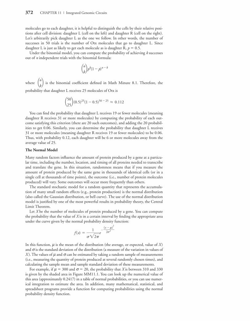
For example, if µ � 300 and σ � 20, the probability that X is between 310 and 330is given by the shaded area in Figure MM11.1. You can look up the numerical value ofthis area (approximately 0.2417) in a table of normal probabilities, or you can use numer-ical integration to estimate the area. In addition, many mathematical, statistical, andspreadsheet programs provide a function for computing probabilities using the normalprobability density function.
e-
(x - m)2
2s2f (x) =
1
s22p
a5025b (0.5)25(1 - 0.5)50 - 25
L 0.112
ankb
ankbpk(1 - p)n - k
CAMPMC11_0805382194.QXD 6/12/06 11:56 AM Page 372

SECTION 11.1 | Natural Gene Circuits 373
only one at a time. Either Z can be occupied, or CG2, butnot both. Both binding sites modify the output of moduleA; Z is responsible for repressing and CG2 for amplifying.Given the noise within the system, two genetically identicalcells (descendants of the same fertilized sea urchin egg) mayhave exactly opposite developmental fates. Noise and sto-chastic genomic circuits help explain why even “identical”human twins have different fingerprints. As a result ofnoise, genetic toggle switches are affected by DNA-bindingsite competition and stochastic production of transcriptionfactors. However, genetic toggle switches are too importantto be determined by noise alone. Toggle switches need afeedback loop that reinforces what was initially a random“decision.”
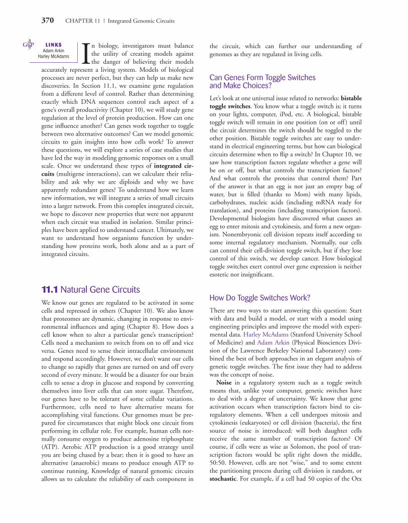
Let’s understand Figure 11.1 (a theoretical switch) beforewe study a naturally occurring toggle switch. Protein A canbind to the cis-regulatory elements of genes b and c to initi-ate transcription for both genes. Protein B has three possi-ble fates: it can be degraded by the cell; it can diffuse awayand perform other functions; and, most importantly for us,it can repress the expression of gene c. Conversely, protein Chas three fates, one of which is to repress gene b. Will pro-tein A bind to b and indirectly suppress c ? Or will A bindto c and suppress b ? Either outcome is possible, because thedetermining factors are stochastic: the amount of A and itsability to find a limited number of binding sites upstreamof b and c. Once the decision is made, a genetically identi-cal population of cells can be split into two subtypes
A handy property of the normal probability distribution is that X is in the interval µ ± σ 67% of the time; X is in the interval µ ± 2σ 95% of the time; and X is in theinterval µ ± 3σ 99% of the time. For example, with µ � 300 and σ � 20, we knowthat X is between 260 and 340 (300 ± 2 × 20) with probability 0.95. We used this prop-erty in Math Minute 8.2 to determine whether a particular node in a graph had anunusually large degree. Because the normal distribution is so often a reasonable approx-imation for random quantities, we can use this property any time we look at data witherror bars to get a rough estimate of the probability that the measured quantity is withinthe interval denoted by the error bars.
Standard stochastic models are excellent starting points for understanding randomcellular processes. However, these models rely on certain assumptions, which may ormay not hold. Like all models, stochastic models can be refined after gathering experi-mental data.
0.005
280 320 340300
0.01
0.015
0.02
1 800
20 2πe
(x�300)2�
Figure MM11.1 Normal probability density function with µ � 300 and σ � 20.The shaded area represents the probability that X is between 310 and 330.
CAMPMC11_0805382194.QXD 6/12/06 11:56 AM Page 373
374 CHAPTER 11 | Integrated Genomic Circuits
(Figure 11.1b). An individual cell will produce only B or C.No cells will make both, nor are there any genetic hard-wiring instructions that allow us to predict which path anyparticular cell will choose.
DISCOVE RY QU ESTIONS1. If two molecules of protein A were inside a single
cell, would it be possible to produce equalamounts of proteins B and C in the same cell?
2. In Figure 11.1b, why did more cells produce pro-tein C than protein B? Would you predict thissame outcome if you repeated the experiment?Explain your answer.
Theory Is Nice, but Do Toggle Switches Really Exist?
Theoretical models help us comprehend general principles,but they are useful only if they approximate reality. Manypathogens evade our immune systems by changing their
protein exteriors on a regular basis. How can genetically iden-tical pathogens present different exteriors? They take advan-tage of noise and toggle switches. As your immune systemlearns to search and destroy, the pathogen changes its appear-ance. For the pathogen, it is easy to see that there are evolu-tionary forces at work to maintain noise and toggle switches,but mechanistically, how does it work? This section discussesseveral naturally evolved circuits and the toggle switches ineach one; Section 11.2 highlights some recent research intosynthetic circuits constructed by investigators but testedinside cells. Both types of research help us measure our under-standing of noise, toggle switches, and biological circuits.
Let’s take a closer look at a naturally evolved toggleswitch that controls the behavior of the bacterial virus calledλ phage. λ has two behaviors from which to “choose.” It caneither live quietly within its Escherichia coli host (lysogeniclifestyle), or it can replicate rapidly and blow up its host asthe progeny are launched to infect new hosts (lyticlifestyle). The choice between peaceful coexistence andlethal parasitism is made by a single protein with the incon-spicuous name of CII (pronounced C two).
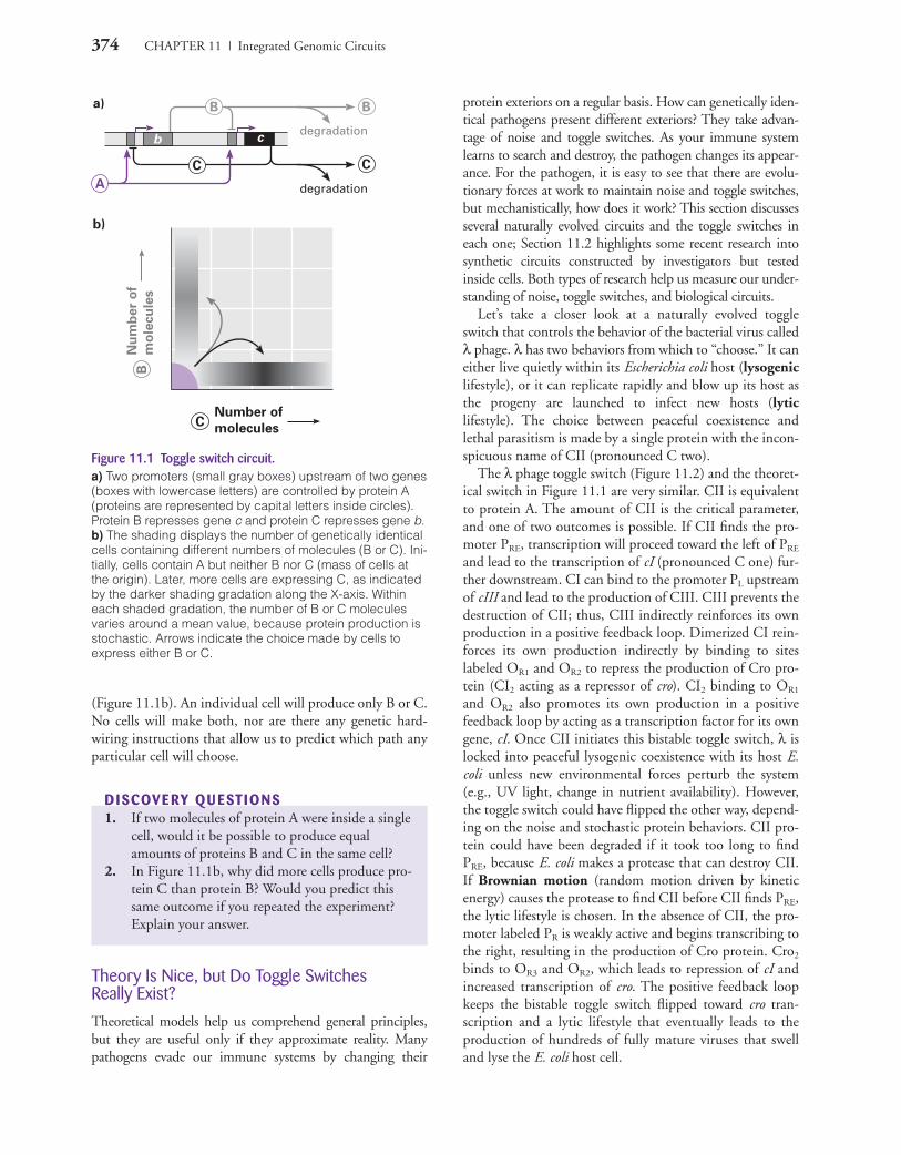
The λ phage toggle switch (Figure 11.2) and the theoret-ical switch in Figure 11.1 are very similar. CII is equivalentto protein A. The amount of CII is the critical parameter,and one of two outcomes is possible. If CII finds the pro-moter PRE, transcription will proceed toward the left of PRE
and lead to the transcription of cI (pronounced C one) fur-ther downstream. CI can bind to the promoter PL upstreamof cIII and lead to the production of CIII. CIII prevents thedestruction of CII; thus, CIII indirectly reinforces its ownproduction in a positive feedback loop. Dimerized CI rein-forces its own production indirectly by binding to siteslabeled OR1 and OR2 to repress the production of Cro pro-tein (CI2 acting as a repressor of cro). CI2 binding to OR1
and OR2 also promotes its own production in a positivefeedback loop by acting as a transcription factor for its owngene, cI. Once CII initiates this bistable toggle switch, λ islocked into peaceful lysogenic coexistence with its host E.coli unless new environmental forces perturb the system(e.g., UV light, change in nutrient availability). However,the toggle switch could have flipped the other way, depend-ing on the noise and stochastic protein behaviors. CII pro-tein could have been degraded if it took too long to findPRE, because E. coli makes a protease that can destroy CII.If Brownian motion (random motion driven by kineticenergy) causes the protease to find CII before CII finds PRE,the lytic lifestyle is chosen. In the absence of CII, the pro-moter labeled PR is weakly active and begins transcribing tothe right, resulting in the production of Cro protein. Cro2
binds to OR3 and OR2, which leads to repression of cI andincreased transcription of cro. The positive feedback loopkeeps the bistable toggle switch flipped toward cro tran-scription and a lytic lifestyle that eventually leads to theproduction of hundreds of fully mature viruses that swelland lyse the E. coli host cell.
Nu
mb
er
of
mo
lecu
les
B
Number of
moleculesC
cb
A
B B
C
degradation
C
degradation
b)
a)
Figure 11.1 Toggle switch circuit.a) Two promoters (small gray boxes) upstream of two genes(boxes with lowercase letters) are controlled by protein A(proteins are represented by capital letters inside circles).Protein B represses gene c and protein C represses gene b.b) The shading displays the number of genetically identicalcells containing different numbers of molecules (B or C). Ini-tially, cells contain A but neither B nor C (mass of cells atthe origin). Later, more cells are expressing C, as indicatedby the darker shading gradation along the X-axis. Withineach shaded gradation, the number of B or C moleculesvaries around a mean value, because protein production isstochastic. Arrows indicate the choice made by cells toexpress either B or C.
CAMPMC11_0805382194.QXD 6/12/06 11:56 AM Page 374

SECTION 11.1 | Natural Gene Circuits 375
Cro2
Cro
CII
CI
CIII
OR3
PRM PREPR
PL
OR2 OR1
cro cII
cIII
cI
λ switch
CII degradation
reactions
CIII inhibits CII
degradation
R3
Cro dimerization
and degradation
reactions
R2
CI dimerization
and degradation
reactions
R1
Cro2
CI2
CI2
Figure 11.2 λ toggle switch that chooses between coexistence and murder.DNA (light purple bands) and promoters (light gray boxes with arrows pointing to theirgenes) from λ phage. Genes are black boxes with white arrows indicating the directionRNA polymerase travels to transcribe the genes. Genes are induced (black arrows) orrepressed ⊥ as indicated. Three regulatory regions (purple boxes labeled R1, R2, andR3) determine the lifestyle “decision” for λ phage. Named circles are proteins, with sub-script 2 indicating dimerization. Arrows into and out of regulatory regions represent a flow of information.
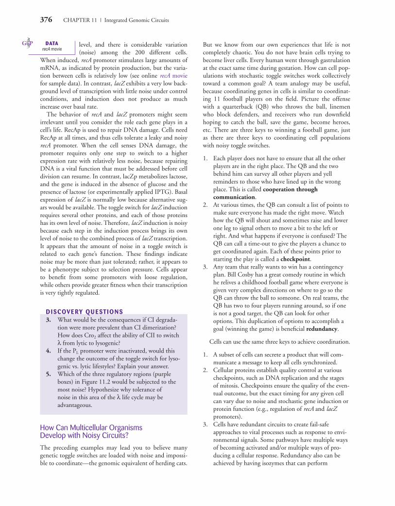
Figure 11.3 Monitoring recA and lacZ pro-moter activity in multiple individual cells.Go to www.GeneticsPlace.com to viewthis figure.
There are several noisy factors in the choice made by λ phage, such as the limited number of proteins and bind-ing sites as well as the variable amount of time it takes toinitiate transcription. Another factor is the burst of proteinproduction. Notice in Figure 11.2 that both Cro and CImust form homodimers to be functional. Dimerization ismore likely to happen when proteins are produced in burststhan when the same number of proteins is made at a slowbut steady rate. A final component worth noting is thatenvironmental influences can skew this decision. For exam-ple, if the bacterium host happens to be growing in a nutri-ent-rich environment (e.g., in a flask with lots of glucose),the bacterium produces more protease, resulting in fasterdestruction of CII and the production of many new λphage (lytic lifestyle). Conversely, if the bacterium hap-pened to be in a nutrient-poor environment (e.g., on thebottom of your shoe), there are fewer (but not zero) pro-tease molecules, so CII has a higher probability of findingits binding site on PRE before being destroyed. A longerhalf-life for CII leads to peaceful coexistence (lysogeniclifestyle), which makes good sense for the virus. Whyshould a virus reproduce rapidly if the environment is notconducive to making more potential hosts? Why not waitfor the nutrients to arrive (e.g., when you step in something
yucky) so the bacteria can grow? When the nutrients arrive,bacteria will grow faster, proteases will be more numerous,CII will be destroyed more readily, more viruses will form,more bacteria will lyse, and viruses will infect more hosts.The selective advantage for a noise-tolerant toggle switch isimpressive.
In recent studies, investigators have examined theamount of noise generated by different aspects of a genomiccircuit. For example, graduate student Yina Kuang in DavidWalt’s Chemistry Department lab at Tufts University led ateam that studied gene expression in single E. coli cells. Theinvestigators placed two different promoters (recA and lacZ )upstream of the reporter gene GFP and then measured theproduction of fluorescence in 200 individual cells wheninduced or under control conditions (Figure 11.3). The recApromoter is constitutively on (always activated) at a low
L I N KSDavid Walt
M ETHODSGFP
CAMPMC11_0805382194.QXD 6/12/06 11:56 AM Page 375
376 CHAPTER 11 | Integrated Genomic Circuits
level, and there is considerable variation(noise) among the 200 different cells.
When induced, recA promoter stimulates large amounts ofmRNA, as indicated by protein production, but the varia-tion between cells is relatively low (see online recA moviefor sample data). In contrast, lacZ exhibits a very low back-ground level of transcription with little noise under controlconditions, and induction does not produce as muchincrease over basal rate.
The behavior of recA and lacZ promoters might seemirrelevant until you consider the role each gene plays in acell’s life. RecAp is used to repair DNA damage. Cells needRecAp at all times, and thus cells tolerate a leaky and noisyrecA promoter. When the cell senses DNA damage, thepromoter requires only one step to switch to a higherexpression rate with relatively less noise, because repairingDNA is a vital function that must be addressed before celldivision can resume. In contrast, lacZp metabolizes lactose,and the gene is induced in the absence of glucose and thepresence of lactose (or experimentally applied IPTG). Basalexpression of lacZ is normally low because alternative sug-ars would be available. The toggle switch for lacZ inductionrequires several other proteins, and each of those proteinshas its own level of noise. Therefore, lacZ induction is noisybecause each step in the induction process brings its ownlevel of noise to the combined process of lacZ transcription.It appears that the amount of noise in a toggle switch isrelated to each gene’s function. These findings indicatenoise may be more than just tolerated; rather, it appears tobe a phenotype subject to selection pressure. Cells appearto benefit from some promoters with loose regulation,while others provide greater fitness when their transcriptionis very tightly regulated.
DISCOVE RY QU ESTIONS3. What would be the consequences if CI degrada-
tion were more prevalent than CI dimerization?How does Cro2 affect the ability of CII to switchλ from lytic to lysogenic?
4. If the PL promoter were inactivated, would thischange the outcome of the toggle switch for lyso-genic vs. lytic lifestyles? Explain your answer.
5. Which of the three regulatory regions (purpleboxes) in Figure 11.2 would be subjected to themost noise? Hypothesize why tolerance of noise in this area of the λ life cycle may be advantageous.
How Can Multicellular Organisms Develop with Noisy Circuits?
The preceding examples may lead you to believe manygenetic toggle switches are loaded with noise and impossi-ble to coordinate—the genomic equivalent of herding cats.
But we know from our own experiences that life is notcompletely chaotic. You do not have brain cells trying tobecome liver cells. Every human went through gastrulationat the exact same time during gestation. How can cell pop-ulations with stochastic toggle switches work collectivelytoward a common goal? A team analogy may be useful,because coordinating genes in cells is similar to coordinat-ing 11 football players on the field. Picture the offensewith a quarterback (QB) who throws the ball, linemenwho block defenders, and receivers who run downfieldhoping to catch the ball, save the game, become heroes,etc. There are three keys to winning a football game, justas there are three keys to coordinating cell populationswith noisy toggle switches.
1. Each player does not have to ensure that all the otherplayers are in the right place. The QB and the twobehind him can survey all other players and yellreminders to those who have lined up in the wrongplace. This is called cooperation through communication.
2. At various times, the QB can consult a list of points tomake sure everyone has made the right move. Watchhow the QB will shout and sometimes raise and lowerone leg to signal others to move a bit to the left orright. And what happens if everyone is confused? TheQB can call a time-out to give the players a chance toget coordinated again. Each of these points prior tostarting the play is called a checkpoint.
3. Any team that really wants to win has a contingencyplan. Bill Cosby has a great comedy routine in whichhe relives a childhood football game where everyone isgiven very complex directions on where to go so theQB can throw the ball to someone. On real teams, theQB has two to four players running around, so if oneis not a good target, the QB can look for otheroptions. This duplication of options to accomplish agoal (winning the game) is beneficial redundancy.
Cells can use the same three keys to achieve coordination.
1. A subset of cells can secrete a product that will com-municate a message to keep all cells synchronized.
2. Cellular proteins establish quality control at variouscheckpoints, such as DNA replication and the stagesof mitosis. Checkpoints ensure the quality of the even-tual outcome, but the exact timing for any given cellcan vary due to noise and stochastic gene induction orprotein function (e.g., regulation of recA and lacZpromoters).
3. Cells have redundant circuits to create fail-safeapproaches to vital processes such as response to envi-ronmental signals. Some pathways have multiple waysof becoming activated and/or multiple ways of pro-ducing a cellular response. Redundancy also can beachieved by having isozymes that can perform
DATArecA movie
CAMPMC11_0805382194.QXD 6/12/06 11:56 AM Page 376
SECTION 11.1 | Natural Gene Circuits 377
b
x
c
BA C
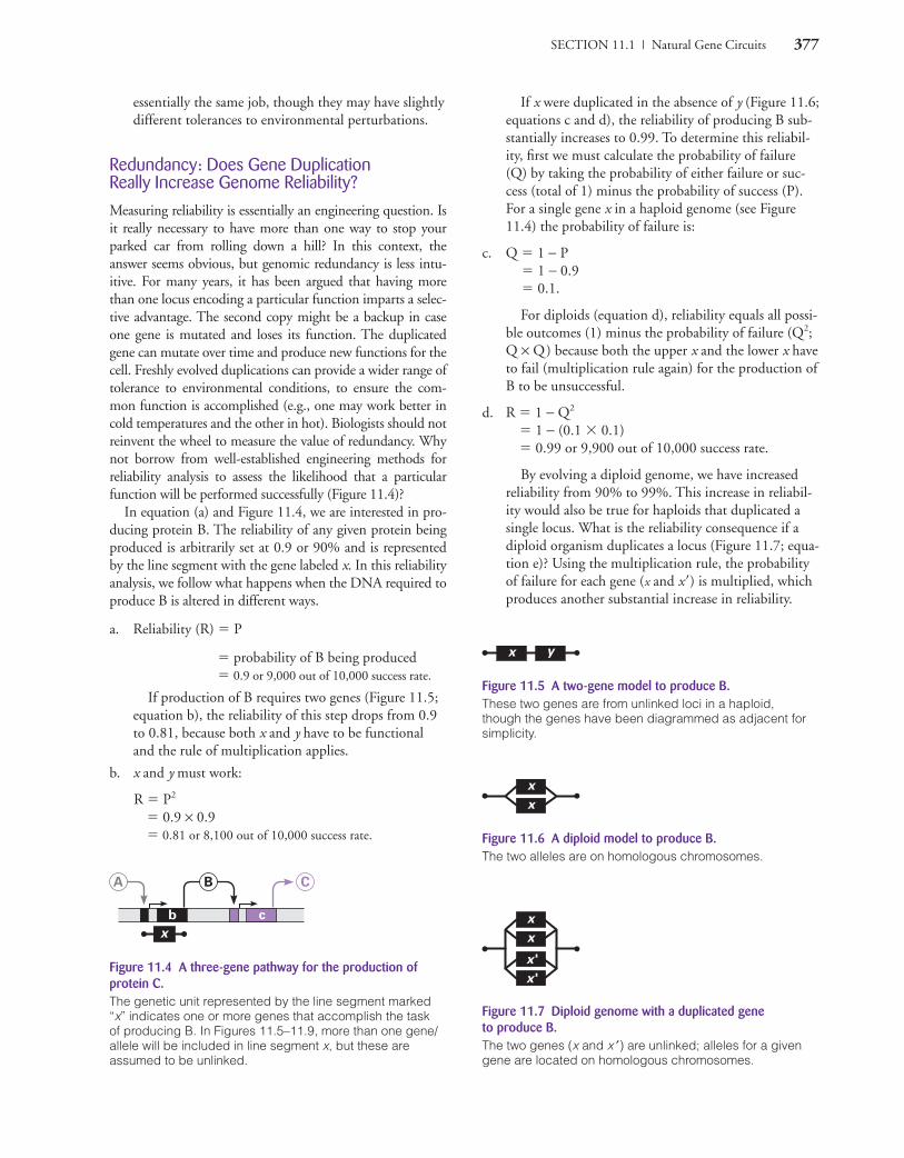
Figure 11.4 A three-gene pathway for the production of protein C.The genetic unit represented by the line segment marked“x” indicates one or more genes that accomplish the task of producing B. In Figures 11.5–11.9, more than one gene/allele will be included in line segment x, but these areassumed to be unlinked.
x y
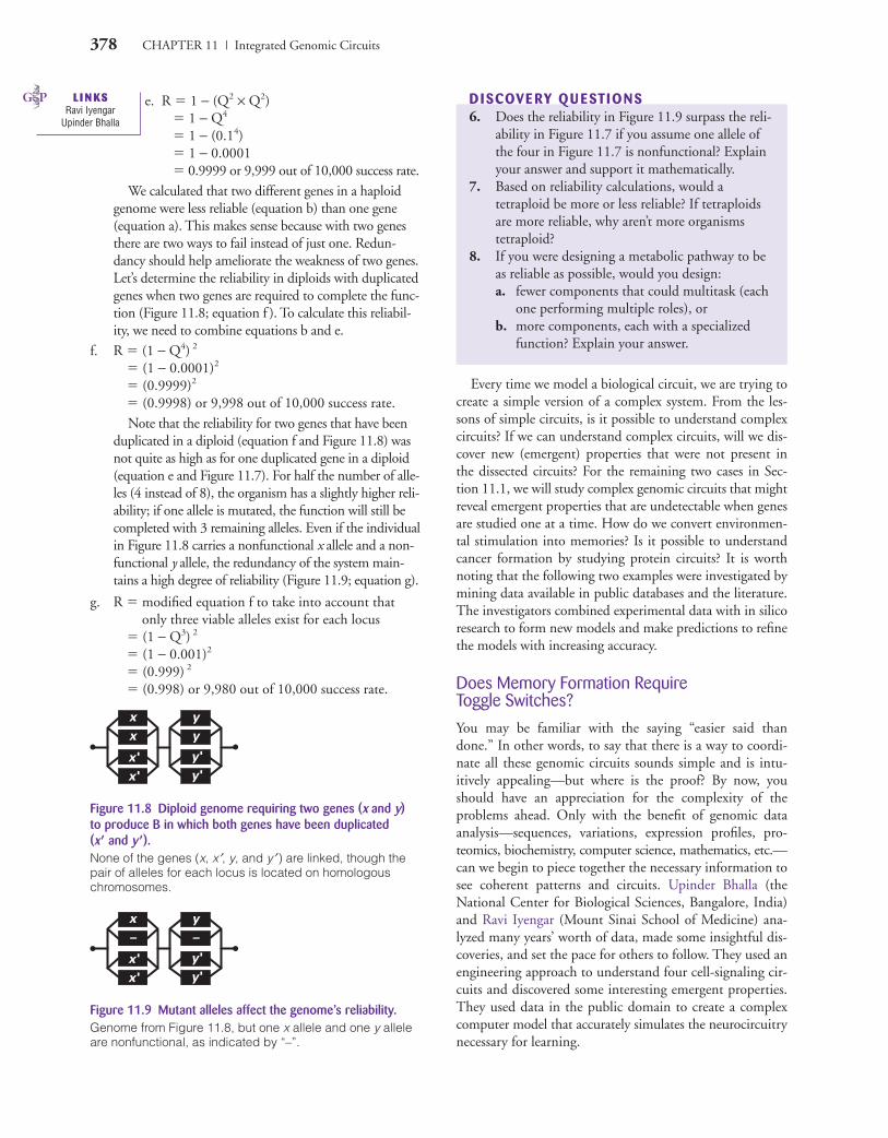
Figure 11.5 A two-gene model to produce B.These two genes are from unlinked loci in a haploid, though the genes have been diagrammed as adjacent forsimplicity.
x
x
Figure 11.6 A diploid model to produce B.The two alleles are on homologous chromosomes.
x '
x '
x
x
Figure 11.7 Diploid genome with a duplicated gene to produce B.The two genes (x and x ′) are unlinked; alleles for a givengene are located on homologous chromosomes.
essentially the same job, though they may have slightlydifferent tolerances to environmental perturbations.
Redundancy: Does Gene Duplication Really Increase Genome Reliability?
Measuring reliability is essentially an engineering question. Isit really necessary to have more than one way to stop yourparked car from rolling down a hill? In this context, theanswer seems obvious, but genomic redundancy is less intu-itive. For many years, it has been argued that having morethan one locus encoding a particular function imparts a selec-tive advantage. The second copy might be a backup in caseone gene is mutated and loses its function. The duplicatedgene can mutate over time and produce new functions for thecell. Freshly evolved duplications can provide a wider range oftolerance to environmental conditions, to ensure the com-mon function is accomplished (e.g., one may work better incold temperatures and the other in hot). Biologists should notreinvent the wheel to measure the value of redundancy. Whynot borrow from well-established engineering methods forreliability analysis to assess the likelihood that a particularfunction will be performed successfully (Figure 11.4)?
In equation (a) and Figure 11.4, we are interested in pro-ducing protein B. The reliability of any given protein beingproduced is arbitrarily set at 0.9 or 90% and is representedby the line segment with the gene labeled x. In this reliabilityanalysis, we follow what happens when the DNA required toproduce B is altered in different ways.
a. Reliability (R) � P
� probability of B being produced� 0.9 or 9,000 out of 10,000 success rate.
If production of B requires two genes (Figure 11.5;equation b), the reliability of this step drops from 0.9to 0.81, because both x and y have to be functionaland the rule of multiplication applies.
b. x and y must work:
R � P2
� 0.9 × 0.9� 0.81 or 8,100 out of 10,000 success rate.
If x were duplicated in the absence of y (Figure 11.6;equations c and d), the reliability of producing B sub-stantially increases to 0.99. To determine this reliabil-ity, first we must calculate the probability of failure(Q) by taking the probability of either failure or suc-cess (total of 1) minus the probability of success (P).For a single gene x in a haploid genome (see Figure11.4) the probability of failure is:
c. Q � 1 − P� 1 − 0.9� 0.1.
For diploids (equation d), reliability equals all possi-ble outcomes (1) minus the probability of failure (Q2;Q × Q) because both the upper x and the lower x haveto fail (multiplication rule again) for the production ofB to be unsuccessful.
d. R � 1 − Q2
� 1 − (0.1 � 0.1)� 0.99 or 9,900 out of 10,000 success rate.
By evolving a diploid genome, we have increasedreliability from 90% to 99%. This increase in reliabil-ity would also be true for haploids that duplicated asingle locus. What is the reliability consequence if adiploid organism duplicates a locus (Figure 11.7; equa-tion e)? Using the multiplication rule, the probabilityof failure for each gene (x and x�) is multiplied, whichproduces another substantial increase in reliability.
CAMPMC11_0805382194.QXD 6/12/06 11:56 AM Page 377
378 CHAPTER 11 | Integrated Genomic Circuits
x '
x '
x
–
y '
y
–
y '
Figure 11.9 Mutant alleles affect the genome’s reliability.Genome from Figure 11.8, but one x allele and one y alleleare nonfunctional, as indicated by “–”.
x '
x '
x
x
y '
y
y
y '
Figure 11.8 Diploid genome requiring two genes (x and y) to produce B in which both genes have been duplicated (x� and y�).None of the genes (x, x′, y, and y′ ) are linked, though thepair of alleles for each locus is located on homologouschromosomes.
e. R � 1 − (Q2 × Q2)� 1 − Q4
� 1 − (0.14)� 1 − 0.0001� 0.9999 or 9,999 out of 10,000 success rate.
We calculated that two different genes in a haploidgenome were less reliable (equation b) than one gene(equation a). This makes sense because with two genesthere are two ways to fail instead of just one. Redun-dancy should help ameliorate the weakness of two genes.Let’s determine the reliability in diploids with duplicatedgenes when two genes are required to complete the func-tion (Figure 11.8; equation f ). To calculate this reliabil-ity, we need to combine equations b and e.
f. R � (1 − Q4) 2
� (1 − 0.0001)2
� (0.9999)2
� (0.9998) or 9,998 out of 10,000 success rate.Note that the reliability for two genes that have been
duplicated in a diploid (equation f and Figure 11.8) wasnot quite as high as for one duplicated gene in a diploid(equation e and Figure 11.7). For half the number of alle-les (4 instead of 8), the organism has a slightly higher reli-ability; if one allele is mutated, the function will still becompleted with 3 remaining alleles. Even if the individualin Figure 11.8 carries a nonfunctional x allele and a non-functional y allele, the redundancy of the system main-tains a high degree of reliability (Figure 11.9; equation g).
g. R � modified equation f to take into account thatonly three viable alleles exist for each locus
� (1 − Q3) 2
� (1 − 0.001)2
� (0.999) 2
� (0.998) or 9,980 out of 10,000 success rate.
DISCOVE RY QU ESTIONS6. Does the reliability in Figure 11.9 surpass the reli-
ability in Figure 11.7 if you assume one allele ofthe four in Figure 11.7 is nonfunctional? Explainyour answer and support it mathematically.
7. Based on reliability calculations, would atetraploid be more or less reliable? If tetraploidsare more reliable, why aren’t more organismstetraploid?
8. If you were designing a metabolic pathway to beas reliable as possible, would you design:a. fewer components that could multitask (each
one performing multiple roles), orb. more components, each with a specialized
function? Explain your answer.
Every time we model a biological circuit, we are trying tocreate a simple version of a complex system. From the les-sons of simple circuits, is it possible to understand complexcircuits? If we can understand complex circuits, will we dis-cover new (emergent) properties that were not present inthe dissected circuits? For the remaining two cases in Sec-tion 11.1, we will study complex genomic circuits that mightreveal emergent properties that are undetectable when genesare studied one at a time. How do we convert environmen-tal stimulation into memories? Is it possible to understandcancer formation by studying protein circuits? It is worthnoting that the following two examples were investigated bymining data available in public databases and the literature.The investigators combined experimental data with in silicoresearch to form new models and make predictions to refinethe models with increasing accuracy.
Does Memory Formation Require Toggle Switches?
You may be familiar with the saying “easier said thandone.” In other words, to say that there is a way to coordi-nate all these genomic circuits sounds simple and is intu-itively appealing—but where is the proof? By now, youshould have an appreciation for the complexity of theproblems ahead. Only with the benefit of genomic dataanalysis—sequences, variations, expression profiles, pro-teomics, biochemistry, computer science, mathematics, etc.—can we begin to piece together the necessary information tosee coherent patterns and circuits. Upinder Bhalla (theNational Center for Biological Sciences, Bangalore, India)and Ravi Iyengar (Mount Sinai School of Medicine) ana-lyzed many years’ worth of data, made some insightful dis-coveries, and set the pace for others to follow. They used anengineering approach to understand four cell-signaling cir-cuits and discovered some interesting emergent properties.They used data in the public domain to create a complexcomputer model that accurately simulates the neurocircuitrynecessary for learning.
L I N KSRavi Iyengar
Upinder Bhalla
CAMPMC11_0805382194.QXD 6/12/06 11:56 AM Page 378
SECTION 11.1 | Natural Gene Circuits 379
G
E
R
k+2
k+1
k–2k–1
G
E
R
k+2
k+1
k–2k–1
G'
E'
R'
k'+2
k'+1
k'–2k'–1
Pairs of interactions: 69Concentrations: 24 Rate constants: 138
Pairs of interactions: 2Concentrations: 3Rate constants: 4
Pairs of interactions: 11Concentrations: 6Rate constants: 22
k +–
k+–
k +–
k+–
G
E
R
k+2
k+1
k–2k–1
G'
E'
E
E'
R'
k'+2
k'+1
k'–2k'–1
k +–
k +–
k +–
k +–
k+–
k +–
k+–
k+–
K
T
C
k+2
k+1
k–2k–1
K'
K
K'
T'
TT'
C'
k'+2
k'+1
k'–2k'–1
k +–
k +–
k +–
k+–
k +–
k+–
k+–
N
P
T
k+2
k+1
k–2k–1
N'
P'
T'
k'+2
k'+1
k'–2k'–1
k +–
k +–
k +–
k+–
k +–
k+–
k+–
c)b)a)
k +–
k +–
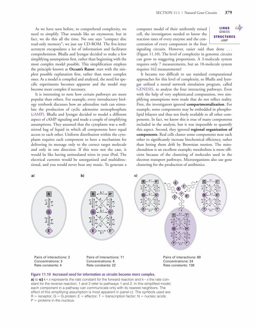
Figure 11.10 Increased need for information as circuits become more complex.a) to c) k�x represents the rate constant for the forward reaction and k�x the rate con-stant for the reverse reaction; 1 and 2 refer to pathways 1 and 2. In this simplified model,each component in a pathway can communicate only with its nearest neighbors. Theeffect of this simplifying assumption is most apparent in panel c). The symbols used are:R � receptor; G � G protein; E � effector; T � transcription factor; N � nucleic acids; P � proteins in the nucleus.
As we have seen before, to comprehend complexity, weneed to simplify. That sounds like an oxymoron, but infact, we do this all the time. No one says “compact discread-only memory”; we just say CD-ROM. The five-letteracronym encapsulates a lot of information and facilitatescomprehension. Bhalla and Iyengar decided to make a fewsimplifying assumptions first, rather than beginning with themost complex model possible. This simplification employsthe principle known as Occam’s Razor: start with the sim-plest possible explanation first, rather than more complexones. As a model is compiled and analyzed, the need for spe-cific experiments becomes apparent and the model maybecome more complex if necessary.
It is interesting to note how certain pathways are morepopular than others. For example, every introductory biol-ogy textbook discusses how an adrenaline rush can stimu-late the production of cyclic adenosine monophosphate(cAMP). Bhalla and Iyengar decided to model a differentaspect of cAMP signaling and made a couple of simplifyingassumptions. They assumed that the cytoplasm was a well-stirred bag of liquid in which all components have equalaccess to each other. Uniform distribution within the cyto-plasm requires each component to have a mechanism fordelivering its message only to the correct target moleculeand only in one direction. If this were not the case, itwould be like having uninsulated wires in your iPod. Theelectrical currents would be unorganized and multidirec-tional, and you would never hear any music. To generate a
computer model of their uniformly mixedcell, the investigators needed to know thereaction rates of every enzyme and the con-centration of every component in the foursignaling circuits. However, easier said than done . . .(Figure 11.10). The level of complexity in genomic circuitscan grow to staggering proportions. A 3-molecule systemrequires only 7 measurements, but an 18-molecule systemrequires 162 measurements!
It became too difficult to use standard computationalapproaches for this level of complexity, so Bhalla and Iyen-gar utilized a neural network simulation program, calledGENESIS, to analyze the four interacting pathways. Evenwith the help of very sophisticated computation, two sim-plifying assumptions were made that do not reflect reality.First, the investigators ignored compartmentalization. Forexample, some components may be embedded in phospho-lipid bilayers and thus not freely available to all other com-ponents. In fact, we know this is true of many componentsincluded in the analysis, but it was impossible to quantifythis aspect. Second, they ignored regional organization ofcomponents. Real cells cluster some components near eachother to significantly increase biochemical efficiency, ratherthan letting them drift by Brownian motion. The mito-chondrion is an excellent example; metabolism is more effi-cient because of the clustering of molecules used in theelectron transport pathways. Microorganisms also use geneclustering for the production of antibiotics.
L I N KSGENESIS
STRUCTU REScAMP
CAMPMC11_0805382194.QXD 6/12/06 11:56 AM Page 379
380 CHAPTER 11 | Integrated Genomic Circuits
Are Simple Models of ComplexCircuits Worthwhile?
Most biologists assume that interconnectedcircuits work synergistically. The existence of synergy is whymany in field biology dislike the reductionist approach usedby molecular biologists. However, the reductionists’ goal isnot merely to disassemble a cell to look at the parts, but tounderstand the parts well enough to explain synergisticinteractions and move beyond descriptions toward testablepredictions. The particular case under investigation was onethat philosophers and biologists have pondered for cen-turies: How do we learn?
Neurobiologists have given us great insights into the mech-anisms utilized whenever an animal (e.g., flies or humans)learns something new. Intuitively, we know our neurons mustundergo some sort of change in order for us to retain infor-mation. There is a genetic component to memory formation,so we know proteins are involved. Somehow, proteins mustalter what a neuron does—become depolarized when stimu-lated and release neurotransmitters to relay this information.Sounds simple, right? A neuron’s change in function is calledlong-term potentiation (LTP), which means the conse-quence of neuronal stimulation is maintained after the origi-nal stimulus is gone. To see a simple example of this, stare ata bright light and then turn away. Even though the light isno longer hitting your neurons, you still “see” it. Your neu-ron’s function was changed so that it performed differentlyafter the stimulus was removed. Bhalla and Iyengar decidedto model the complex circuitry of the mammalian brain.
Before we begin dissecting, we need to learn a little brainanatomy to provide the context for learning. Where in thebrain does learning taking place? Deep within your cere-brum is a collection of neurons called the hippocampus.For at least 30 years, memory research has focused on thehippocampus as the center of learning/memory. Inside thehippocampus are layers of neurons, and each layer has aname. We will focus on the CA1 layer. On the cell body anddendrite of CA1 neurons are bumps called spines. Embed-ded in these spines are integral membrane proteins, three ofwhich are of particular interest to us. The neurotransmitterglutamate binds to its receptor, called mGluR (mouseglutamate receptor). As with all receptors, it facilitates signaltransduction; that is, it transmits the extracellular signal acrossthe plasma membrane. NMDAR (N-methyl-D-aspartatereceptor) is a voltage-sensitive calcium ion channel. Thefinal plasma membrane component is AMPAR (α-amino-3-hydroxy-5-methyl-4-isoxazolepropionate receptor), anotherglutamate receptor that acts as an ion channel when stimu-lated by glutamate. LTP is initiated when mGluR andNMDAR are stimulated by a certain amount and frequencyof stimuli. Experimentally, LTP can be induced in mouseneurons when stimulated with 3 mild electrical inputs of100 Hz pulses, 1 second each and separated by 10 minutes.Bhalla and Iyengar set out to construct a computer model ofthe complex series of events from stimulation to LTP.
How Much Math Is Required to Model Memory?
Molecular biology is becoming mature enough to need theassistance of many other disciplines, especially mathematics.However, the math used in this study is quite simple. Tostart their in silico research, Bhalla and Iyengar consideredonly two types of connections: protein-protein interactionsand second messengers. Two additional facts they consid-ered were: (1) proteins degrade, that is, they are destroyedby the cell over time; and (2) enzymes have reaction rates—for example, there is an average amount of time it takes akinase to consume ATP and add a phosphate onto its sub-strate. In the first reaction below, A and B join to form AB.This illustrates how two proteins, such as a kinase and itsprotein substrate, can bind to each other. The binding has aforward reaction rate (kf ) and a backward reaction rate (kb).The second reaction shows the conversion of A and B intoC and D. For example, we could measure the amount ofNa� inside a cell (A) and the amount of K� outside a cell(B) as they are changed into Na� outside a cell (C) and K�
inside a cell (D). The forward rate of this conversion (kf ) isthe rate of the Na/K pump, and the backward rate (kb) is therate of ions passing through ion channels. This second reac-tion can be written as an equation, which says that thechange (d ) in the concentration of A ([A]) over a change intime (/dt) is equal to the production of A (the backward ratetimes the concentrations of C and D, which is written: kb
[C][D]) minus the amount of A lost (due to the forwardreaction that consumes A, which is written: kf [A][B]). Youhave studied these types of interactions and rates before,so this level of circuitry should be comprehensible so far.The math is only multiplication, division, and subtraction.To determine LTP, all we need is numbers to replace thevariables.
One more enzymatic interaction is needed to analyze thelearning circuit. The next equation states that an enzyme(E) binds to its substrate (S) to form a complex of the two(ES). This step can go forward (k1) or backward (k2), mean-ing the reaction is reversible. However, the second step isirreversible, as indicated by the forward arrow and only onerate constant (k3). Therefore, the ES complex can be con-verted into the original enzyme (E; an enzyme is never con-sumed in a reaction) plus a new product (P). Each stepoccurs at a measurable rate, and these values are called rateconstants (the k values). For example, the enzyme adenylylcyclase produces cAMP from the substrate ATP. Adenylylcyclase (E) binds to ATP (S) and forms (at rate k1) a com-plex of the two (ES). ATP and adenylyl cyclase can fall
d[A]/dt = kb[C ][D] - kf [A][B]
A + Bkf
∆
kb
C + DA + Bkf
∆
kb
AB
L I N KSlong-term potentiation
M ETHODSbrain anatomy
CAMPMC11_0805382194.QXD 6/12/06 11:56 AM Page 380
SECTION 11.1 | Natural Gene Circuits 381
apart (k2) or proceed (k3) toward an irreversible productionof adenylyl cyclase plus cAMP (P).
That’s all the math and chemistry you need to under-stand to grasp this very sophisticated in silico analysis oflearning! We still have one problem, though. We don’t haveany real numbers to put into these equations. Luckily, bio-chemists and cell biologists have published all the valuesneeded to initiate a GENESIS software analysis of a nerve’sability to learn.
How Do You Build Complex Models?
Fifteen well-studied circuits were needed to produce Bhallaand Iyengar’s LTP simulation (Figure 11.11). They started bybuilding computer models of each of the 15 circuits individ-ually. At each step, they made sure that the models matchedexperimental data. This alone was an impressive task, buthere is where the fun starts. They began to build integratedcircuits by gradually combining each of the 15 individual cir-cuits. Initially, they only allowed two types of connectionsbetween circuits: (1) secondary messengers arachidonic acid(AA) and diacylglycerol (DAG), and (2) an enzyme in onecircuit bound to its substrate produced in another circuit.
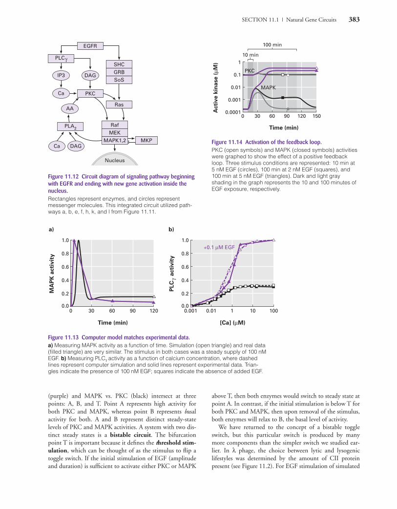
Permitting these two types of interactions allowed theinvestigators to combine the circuits labeled a, b, e, f, h, k,and l in Figure 11.11 into one integrated circuit (Fig-ure 11.12). Notice that epidermal growth factor (EGF)leads to the activation of two enzymes: mitogen-associatedprotein kinase (MAPK) (in circuit a) and PLCγ (in circuitf ). MAPK has been studied intensively for many years. It isassociated with substances that stimulate mitosis, and itphosphorylates proteins. Loss of control of MAPK can leadto the formation of cancerous cells. PLCγ is one isoform, orversion, of phospholipase-C (there are several PLC genes ineach person, and this version, or isoform, is called γ) thatcuts the phospholipid called phosphotidyl inositol bisphos-phate (PIP2) into inositol trisphosphate (IP3) and diacyl-glycerol (DAG). By connecting these seven circuits, a newlayer of complexity became evident—feedback loops. Afeedback loop occurs when the product has a stimulatoryor inhibitory effect on one of the upstream components,such as an enzyme that leads to product formation.
Can a Transient Stimulus Produce Persistent Kinase Activation?
Do individual circuits behave synergistically when they areintegrated into a larger pathway? Can a computer modelaccurately simulate LTP? Can we use this model to makepredictions that lead to improved understanding of how welearn new information? We know that these individualcomponents and circuits are involved in learning, and we
E + Sk1
∆
k2
ES :k3
E + P
know that LTP is the result of long-termactivation of a kinase. But is it really possi-ble to simulate something as complex as learning on a fewmegabytes of computer microcircuits?
How did the computer model compare with real data? InFigure 11.13a, you can see the simulation approximatedthe experimental data. In this graph, the MAPK activitywas plotted as a function of time (d [A]/dt ). The activationof MAPK was transient due to the normal degradationmechanisms in the cell. Equally impressive is Figure11.13b, comparing simulated PLCγ activity (dashed lines)with experimental data (solid lines) in the presence (trian-gles) or absence (squares) of EGF over a 10,000-fold rangeof calcium concentrations. Given the close agreementbetween experimental data and the computer model, thesetwo investigators had a good foundation on which to buildmore complex integrated circuits.
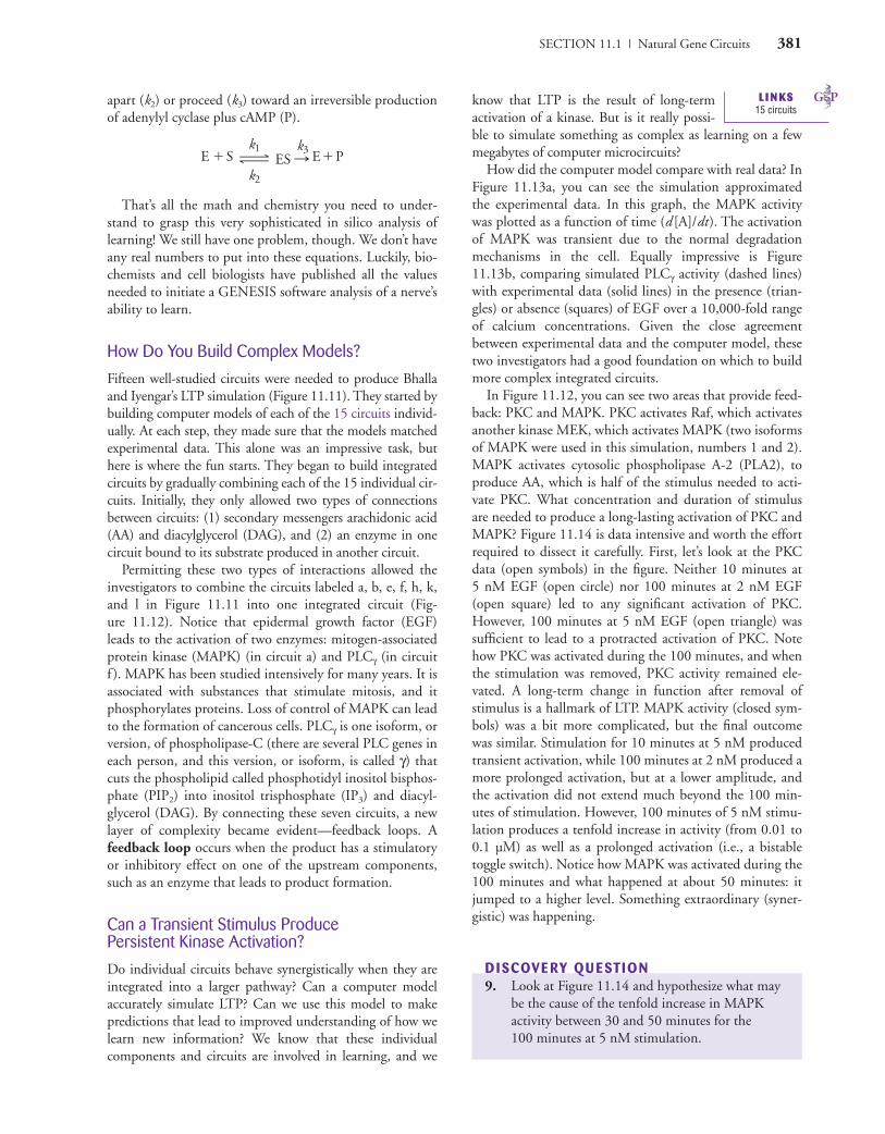
In Figure 11.12, you can see two areas that provide feed-back: PKC and MAPK. PKC activates Raf, which activatesanother kinase MEK, which activates MAPK (two isoformsof MAPK were used in this simulation, numbers 1 and 2).MAPK activates cytosolic phospholipase A-2 (PLA2), toproduce AA, which is half of the stimulus needed to acti-vate PKC. What concentration and duration of stimulusare needed to produce a long-lasting activation of PKC andMAPK? Figure 11.14 is data intensive and worth the effortrequired to dissect it carefully. First, let’s look at the PKCdata (open symbols) in the figure. Neither 10 minutes at 5 nM EGF (open circle) nor 100 minutes at 2 nM EGF(open square) led to any significant activation of PKC.However, 100 minutes at 5 nM EGF (open triangle) wassufficient to lead to a protracted activation of PKC. Notehow PKC was activated during the 100 minutes, and whenthe stimulation was removed, PKC activity remained ele-vated. A long-term change in function after removal ofstimulus is a hallmark of LTP. MAPK activity (closed sym-bols) was a bit more complicated, but the final outcomewas similar. Stimulation for 10 minutes at 5 nM producedtransient activation, while 100 minutes at 2 nM produced amore prolonged activation, but at a lower amplitude, andthe activation did not extend much beyond the 100 min-utes of stimulation. However, 100 minutes of 5 nM stimu-lation produces a tenfold increase in activity (from 0.01 to0.1 µM) as well as a prolonged activation (i.e., a bistabletoggle switch). Notice how MAPK was activated during the100 minutes and what happened at about 50 minutes: itjumped to a higher level. Something extraordinary (syner-gistic) was happening.
DISCOVE RY QU ESTION9. Look at Figure 11.14 and hypothesize what may
be the cause of the tenfold increase in MAPKactivity between 30 and 50 minutes for the 100 minutes at 5 nM stimulation.
L I N KS15 circuits
CAMPMC11_0805382194.QXD 6/12/06 11:56 AM Page 381

382 CHAPTER 11 | Integrated Genomic Circuits
Why Does 100 Minutes of 5 nM EGF Achieve Long-Term Activation?
For the toggle switch of long-term enzyme activation,determining the importance of a particular combinationof EGF concentration and duration of exposure is morecomplex than you might imagine at first. If MAPK couldbe transiently activated after 10 minutes at 5 nM or
100 minutes at 2 nM, then why were these levels of MAPKactivation insufficient stimulus to create long-term activation?To determine the answer, we need to analyze Figure 11.15.
These two activity plots were generated by theconcentration-effect curves for MAPK activation of PKC(purple line) and PKC activation of MAPK (black line),plotted on the same axes. The curves for PKC vs. MAPK
a)
d)
j)
m)n) o)
k)
e)
f)
l)
h) i)
g)
b)c)
EGF.EGFR_INTERNALEGF.EGFREGF + EGFR1
5
2
6
3
8 9
4SHC SHC*
GDP.Ras GTP.Ras
SHC*.SOS.GRB2SOS.GRB2SOS + GRB2
10SOS*.GRB2SOS* + GRB2
7MAPK*
AC1/8Gs.Ac1/81
2cAMP ATP
4cAMP ATP
87
AC2*
PKC
Deph.
GsαCa4.CaM.AC1/8
3Ca4.CaM
16Ca4.CaM
AC2Gs.Ac25
6cAMP ATP
119cAMP ATPATP
1213
PDE*
PKA
Deph.PDE
15AMPcAMP
18AMPcAMP
14AMP cAMP
PDE1 Ca4.CaM.PDE117
cAMP
Gsα
10Gs.AC2*1
2GEF* GEF
129
13
GTP.Ras
GDP.Ras
GAP
inact
PKA
3
4GAP GAP*
PKC
Deph.
6
8
5
7GEF*
PKC
Deph.Deph.
Ca4.CaM
Gβγ
Gβγ.GEF
CaM.GEF
1210 13
GTP.Ras
GAP
1211 13
GDP.Ras
GAP
7
1
2
3
5
6
4
9
Gαβγ–R
Glu–R Gαβγ–Glu–R
Gαβγ + R
8
Synapse
Glu
Gα–GDP Gα–GTP
Gβγ
Gαβγ
Gβγ
Glu
GTP
GTP
GDP
Gαβγ
Ca.PLCγPLCγ3
4 EGF.EGFR
PIP
2PIP2 DAG + IP3
1Ca
PLCγ*5Ca
Ca.PLCγ*
DAG + IP3
Deph.
6
PIP2
PIP2
1
2
CaPLC Ca–PLC
3 45
6
7
CaGq–PLC Ca–Gq–PLC
GqGq
8DAG PC
9IP3 Inositol
G*GDP DAG + IP3
1 2
5
GTP.Ras
MAPKtyr*
MAPKK**
MKP1
MAPK MAPK*
MAPKK**
MKP1
PP2–A PP2–A
Raf*
PKC
Raf Raf**
MAPK*
MAPKK*
GTP.Ras.Raf*
PP2–A
MAPKK MAPKK**
PP2–A
3 4
6 7
8 9
10 11
12 13
Deph.MAPK
AA13
12APC
AA13
8APC
AA13
4APC
AA13
6APC
AA13
2
1
3
APC
Ca–PLA2*
PLA2*
DAG–Ca–PLA2
Ca–PLA2PLA2–cyt.
PIP2–Ca–PLA2
PIP2–PLA2
DAG
PIP2*PIP2*
Ca
Ca
5
11
7
9
10
Ca2.CaMCaM12 Ca
Ca3.CaM2Ca
Ca4.CaM3Ca
Ng.CaM Ng* + CaM
Ng
4
CaM.Can.Ca4.PP2B
PKC
Ng*Deph.
5
67
8
CaM.CaMKII*thr286
PP1
PP1
PP1
CaMKII_a
Ca4.CaM
1
2,3,4,5
CaMKII
CaM.CaMKII
CaMKII**
Ca4.CaM
CaMKII*thr286
CaMKII*inact
PP1
CaMKII
CaM.CaMKIICaM.CaMKII*thr286
CaMKII*thr286
CaMKII**
Basa1_act
6
PP1CaMKII_a10,11,12,13
14
7
8
9
15
16
cAMP4.R2C
R2C2
cAMP.R2C2
cAMP1 PKA_a
PKA_inhib.PKA
PKA_inhib
7
cAMP2.R2C2
cAMP2
cAMP3.R2C2
cAMP3
cAMP4.R2
cAMP4.R2C2
cAMP4
5
6PKA_a
DAG.PKC
PKC–i
10AA 6AA.DAG.PKC
DAG.Ca.PKC
PKC–a
5PKC–a
4PKC–a
3PKC–a
9
Ca.PKC
DAGAA
2PKC–a
1PKC–a
AA
Basa1
7
8
Ca
DAG
4Ca3.CaM
Ca4.CaM
Ca2.CaM
Ca4.PP2B Ca3.CaM.Ca4.PP2B
Ca2.PP2B
2 Ca
2
2 Ca
1
PP2B
Ca2.CaM.Ca4.PP2B
5
Ca4.CaM.Ca4.PP2B
3
Cap_Channel
2 Ca_Stores
8
Ca_pump1
2
4
Leak
Ca_ext Ca Ca_Stores3
5
Leak
IP3R*Cap_Channel*
IP3R
3 IP39
Ca_transp
2 Ca
7
6
Ca2.Ca_transp
PP1–a2 3
I1I1 I1*
I1*.PP1 I1.PP1
CaM.Can.Ca4.PP2BPP2A
PP2A
Ca4.PP2BPKA
I1I1*
1
4
56
7 8
Gsα
Figure 11.11 The 15 circuits that were modeled individually before being integrated intomore complex networks.Reversible reactions are indicated by double-headed arrows. Enzyme reactions aredrawn as curved arrows, with the enzyme listed in the middle. For visual clarity, anycomponent may be present more than once in a single circuit.
CAMPMC11_0805382194.QXD 6/12/06 11:56 AM Page 382
SECTION 11.1 | Natural Gene Circuits 383
0.0
0.4
0 6030 90 120
0.2
0.6
0.8
1.0
Time (min)
MA
PK
acti
vit
y
0.0
0.4
0.001 10.01 10 100
0.2
0.6
0.8
1.0
[Ca] (µM)
PL
Cγ
acti
vit
y
a) b)
+0.1 µM EGF
10 min
PKC
MAPK
100 min
0.0001
0.01
0 9030 60 120 150
0.001
0.1
1
Time (min)
Acti
ve
kin
ase
(µM
)
Figure 11.14 Activation of the feedback loop.PKC (open symbols) and MAPK (closed symbols) activitieswere graphed to show the effect of a positive feedbackloop. Three stimulus conditions are represented: 10 min at 5 nM EGF (circles), 100 min at 2 nM EGF (squares), and100 min at 5 nM EGF (triangles). Dark and light gray shading in the graph represents the 10 and 100 minutes ofEGF exposure, respectively.
EGFR
DAG
DAG
SHCPLCγ
PKC
IP3GRBSoS
MAPK1,2 MKPMEKRaf
AA
Nucleus
Ca
Ca
Ras
PLA2
Figure 11.12 Circuit diagram of signaling pathway beginningwith EGFR and ending with new gene activation inside thenucleus.Rectangles represent enzymes, and circles represent messenger molecules. This integrated circuit utilized path-ways a, b, e, f, h, k, and l from Figure 11.11.
Figure 11.13 Computer model matches experimental data.a) Measuring MAPK activity as a function of time. Simulation (open triangle) and real data(filled triangle) are very similar. The stimulus in both cases was a steady supply of 100 nMEGF. b) Measuring PLCγ activity as a function of calcium concentration, where dashedlines represent computer simulation and solid lines represent experimental data. Trian-gles indicate the presence of 100 nM EGF; squares indicate the absence of added EGF.
(purple) and MAPK vs. PKC (black) intersect at threepoints: A, B, and T. Point A represents high activity forboth PKC and MAPK, whereas point B represents basalactivity for both. A and B represent distinct steady-statelevels of PKC and MAPK activities. A system with two dis-tinct steady states is a bistable circuit. The bifurcationpoint T is important because it defines the threshold stim-ulation, which can be thought of as the stimulus to flip atoggle switch. If the initial stimulation of EGF (amplitudeand duration) is sufficient to activate either PKC or MAPK
above T, then both enzymes would switch to steady state atpoint A. In contrast, if the initial stimulation is below T forboth PKC and MAPK, then upon removal of the stimulus,both enzymes will relax to B, the basal level of activity.
We have returned to the concept of a bistable toggleswitch, but this particular switch is produced by manymore components than the simpler switch we studied ear-lier. In λ phage, the choice between lytic and lysogeniclifestyles was determined by the amount of CII proteinpresent (see Figure 11.2). For EGF stimulation of simulated
CAMPMC11_0805382194.QXD 6/12/06 11:56 AM Page 383

384 CHAPTER 11 | Integrated Genomic Circuits
A
T
B
MAPK vs. PKCPKC vs. MAPK
0
0.1
0.01 1 100.1 100 1000
0.2
0.3
0.4
[MAPK] (nM)
[PK
C]
(µM
)
Figure 11.15 Bistability plot for feedback loop in Figure 11.12.The PKC vs. MAPK activities plot (purple line) was con-structed by holding the level of active MAPK constant, run-ning the simulation until steady state, and reading the valuefor active PKC. This process was continued for a series ofMAPK levels spanning the range of interest. A similarprocess was repeated for MAPK vs. PKC activities plot(black line) by holding the level of active PKC constant andcalculating MAPK activity. Both plots were drawn with theconcentrations of PKC on the Y-axis and MAPK on the X-axis. The curves intersect at three points: B (basal), T (threshold), and A (active). A and B are stable points, but T is the toggle switch point for the two steady-state“choices” of A and B.
Math Minute 11.2 Is It Possible to Predict Steady-State Behavior?
Figure 11.15 depicts the steady-state MAPK concentration when [PKC] is held con-stant (black line), and the steady-state PKC concentration when [MAPK] is held con-stant (purple line). If we want to know the response of MAPK to a particularconcentration of PKC, we begin at that value on the PKC axis, move horizontally untilwe hit the black line, move vertically until we hit the MAPK axis, and read the concen-tration at the point where we hit the MAPK axis. Conversely, if we want to know theresponse of PKC to a particular concentration of MAPK, we begin at that value on theMAPK axis, move vertically until we hit the purple line, move horizontally until wehit the PKC axis, and read the concentration at the point where we hit the PKC axis.Note that A, T, and B are stable points; if [PKC] or [MAPK] is at one of these threepoints, the response of the other kinase is at that same point.
You can analyze the stability of the feedback loop between MAPK and PKC by itera-tively determining the response of [MAPK] to [PKC] and the response of [PKC] to[MAPK]. The assumption behind this iterative process is that [MAPK] at a particulartime depends on [PKC] at an earlier time. Likewise, [PKC] at a particular time dependson [MAPK] at an earlier time. A graphical technique known as a cobweb diagram ishelpful in following the iterative process.
Figure MM11.2 illustrates a cobweb diagram for an initial value of [MAPK] justabove the threshold T, about halfway between 10 and 100 nM ([MAPK] ≈ 101.5 ≈32 nM). From this point on the MAPK axis, move vertically to the purple line and hor-izontally to the [PKC] axis. As described earlier, the resulting point (approximately 0.23 µM) is the response of PKC to the initial MAPK concentration. MAPK will nowrespond to this value (0.23 µM) of [PKC]. The resulting [MAPK] (approximately
LTP, a critical level of kinase activity in a positive feedbackloop determines whether the stimulus leads to LTP (i.e.,learning) or not.
Bhalla and Iyengar made an interesting analogy that wasvery appropriate given that they were simulating learning.They reminded us that a bistable (i.e., digital) system canstore information the same way that RAM stores informa-tion on a computer. It is also worth noting that the simu-lated enzymatic bistable system was very reliable, due to theredundant mechanisms for achieving steady-state level A.High activity of either PKC or MAPK was sufficient to flipthe system from off (steady-state B) to on (steady-state A).Earlier, we described biological systems in engineeringterms, including “redundant,” “reliable,” and “fail-safe.”Another engineering term, robust, means the circuit toler-ates a wide range of environmental conditions. Accordingto data not shown here, when the activities of five differentenzyme concentrations were varied (PKC, MAPK, Raf,PLA2, and MAPKK, which phosphorylates MAPK to acti-vate it), the simulated bistable circuit remained functional.An interesting consequence of this analysis was that most ofthe permutations were equally effective in achieving steady-state A, but PKC was the least tolerant to change, indicat-ing it was the least robust enzyme of the five tested. Theinvestigators hypothesized that PKC’s lack of robustnesswas due to a limited number of PKC isoforms in theircomputer simulation (i.e., too little redundancy).
CAMPMC11_0805382194.QXD 6/12/06 11:56 AM Page 384

SECTION 11.1 | Natural Gene Circuits 385
A
T
B
0
0.1
0.01 1 100.1 100 1000
0.2
0.3
0.4
[MAPK] (nM)
[PK
C]
(µM
)
MAPK vs. PKCPKC vs. MAPK
Start
Figure MM11.2 Cobweb diagram of MAPK and PKC concentration response curves.Start by determining the response of [PKC] to 32 nM [MAPK], and repeat this processwith MAPK’s response to the new PKC concentration, and so on, until converging to apoint (e.g., point A).
100 nM) is found by moving horizontally from 0.23 �M on the PKC axis to the blackline, and vertically to the MAPK axis. Repeat the process to find the following succes-sive concentration responses: [PKC] � 0.31 µM; [MAPK] � 200 nM (point A); [PKC] �0.35 µM (point A). The diagram, and thus the concentration of both kinases, has con-verged to A, as was observed in Figure 11.14.
You may have noticed that the lines from the curves to the axes were merely for keep-ing track of the concentrations of each kinase, and are always backtracked in the nextkinase response determination. Therefore, the cobweb diagram can be constructed bybeginning at [MAPK] � 32, moving vertically to the purple line, horizontally to theblack line, vertically to the purple line, and so on, until the diagram converges to A.
You can construct cobweb diagrams starting at various values of [MAPK]. If you beginat [MAPK] � T, the diagram should converge to A, but if you begin at [MAPK] � T,it should converge to B. This shows that T is a threshold stimulation level. Given con-centration-effect curves like those in Figure 11.15, cobweb diagrams allow us to predictthe behavior of systems like this feedback loop.
DISCOVE RY QU ESTIONS10. Design an experiment that allows you to test the
prediction that robust LTP (i.e., learning)requires more than one isoform of PKC.
11. Describe how the variation in different isoformsof PKC relates to the equations we used to calcu-late reliability (see pages 377–378).
12. How do the terms “robust” and “reliability” relateto each other in Figure 11.12?
Can the Modeled Circuit AccommodateLearning and Forgetting?
Although we are oversimplifying what is required to form amemory in your brain, LTP is one critical step. If LTPrequires the long-term activation of either PKC or MAPK,is it ever possible to inactivate these kinases and turn offLTP (i.e., forget a memory)? Bhalla and Iyengar added thisaspect of learning to their already successful model. MAPKmust be phosphorylated (by MAPKK) to be activated; to
CAMPMC11_0805382194.QXD 6/12/06 11:56 AM Page 385
386 CHAPTER 11 | Integrated Genomic Circuits
Acti
ve k
inase (
µM)
10 min
20 min
00 402010 30 50 60
0.1
0.2
0.3
0.4
Time (min)
PKC
MAPK
a)
11 10010 1000
10
100
1000
[MK
P]
(nM
)Time (min)
b)
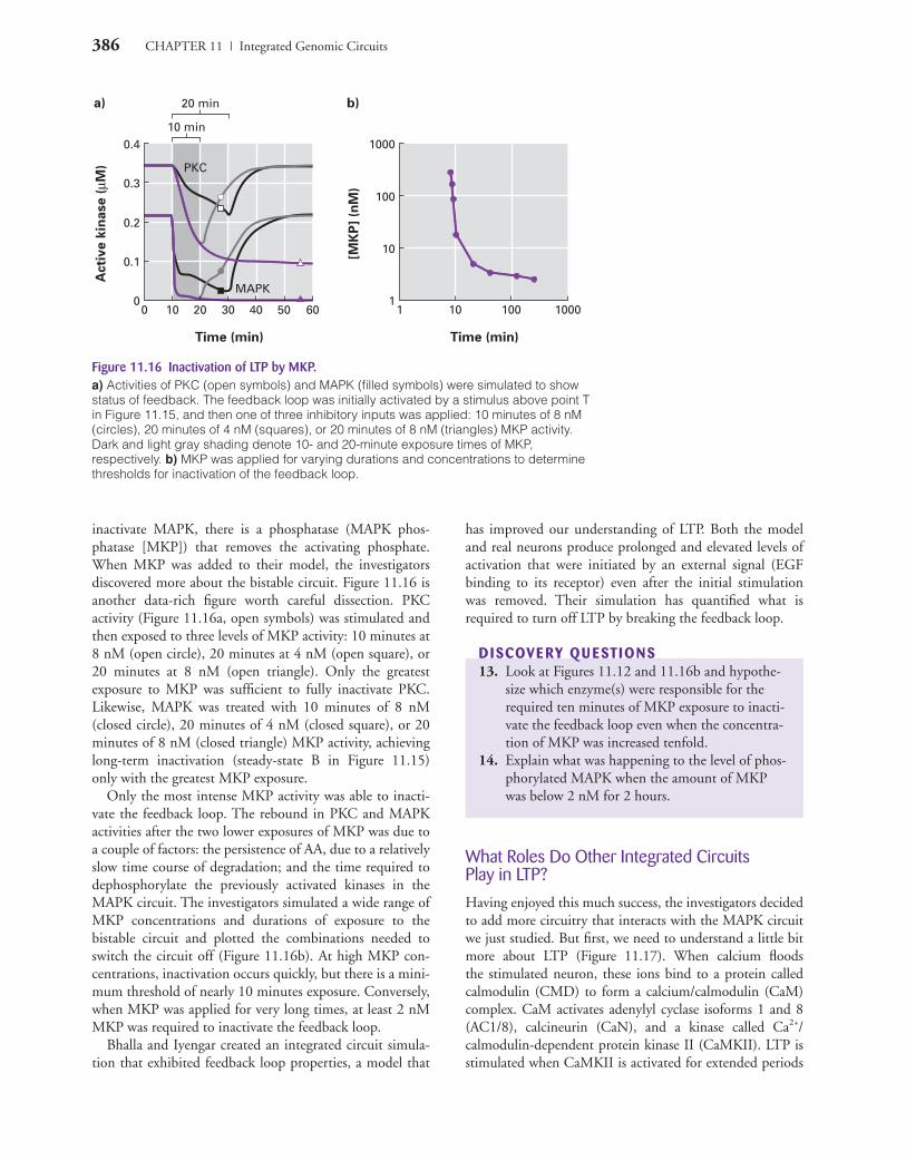
Figure 11.16 Inactivation of LTP by MKP.a) Activities of PKC (open symbols) and MAPK (filled symbols) were simulated to showstatus of feedback. The feedback loop was initially activated by a stimulus above point Tin Figure 11.15, and then one of three inhibitory inputs was applied: 10 minutes of 8 nM(circles), 20 minutes of 4 nM (squares), or 20 minutes of 8 nM (triangles) MKP activity.Dark and light gray shading denote 10- and 20-minute exposure times of MKP, respectively. b) MKP was applied for varying durations and concentrations to determinethresholds for inactivation of the feedback loop.
inactivate MAPK, there is a phosphatase (MAPK phos-phatase [MKP]) that removes the activating phosphate.When MKP was added to their model, the investigatorsdiscovered more about the bistable circuit. Figure 11.16 isanother data-rich figure worth careful dissection. PKCactivity (Figure 11.16a, open symbols) was stimulated andthen exposed to three levels of MKP activity: 10 minutes at8 nM (open circle), 20 minutes at 4 nM (open square), or20 minutes at 8 nM (open triangle). Only the greatestexposure to MKP was sufficient to fully inactivate PKC.Likewise, MAPK was treated with 10 minutes of 8 nM(closed circle), 20 minutes of 4 nM (closed square), or 20minutes of 8 nM (closed triangle) MKP activity, achievinglong-term inactivation (steady-state B in Figure 11.15)only with the greatest MKP exposure.
Only the most intense MKP activity was able to inacti-vate the feedback loop. The rebound in PKC and MAPKactivities after the two lower exposures of MKP was due toa couple of factors: the persistence of AA, due to a relativelyslow time course of degradation; and the time required todephosphorylate the previously activated kinases in theMAPK circuit. The investigators simulated a wide range ofMKP concentrations and durations of exposure to thebistable circuit and plotted the combinations needed toswitch the circuit off (Figure 11.16b). At high MKP con-centrations, inactivation occurs quickly, but there is a mini-mum threshold of nearly 10 minutes exposure. Conversely,when MKP was applied for very long times, at least 2 nMMKP was required to inactivate the feedback loop.
Bhalla and Iyengar created an integrated circuit simula-tion that exhibited feedback loop properties, a model that
has improved our understanding of LTP. Both the modeland real neurons produce prolonged and elevated levels ofactivation that were initiated by an external signal (EGFbinding to its receptor) even after the initial stimulationwas removed. Their simulation has quantified what isrequired to turn off LTP by breaking the feedback loop.
DISCOVE RY QU ESTIONS13. Look at Figures 11.12 and 11.16b and hypothe-
size which enzyme(s) were responsible for therequired ten minutes of MKP exposure to inacti-vate the feedback loop even when the concentra-tion of MKP was increased tenfold.
14. Explain what was happening to the level of phos-phorylated MAPK when the amount of MKPwas below 2 nM for 2 hours.
What Roles Do Other Integrated Circuits Play in LTP?
Having enjoyed this much success, the investigators decidedto add more circuitry that interacts with the MAPK circuitwe just studied. But first, we need to understand a little bitmore about LTP (Figure 11.17). When calcium floodsthe stimulated neuron, these ions bind to a protein calledcalmodulin (CMD) to form a calcium/calmodulin (CaM)complex. CaM activates adenylyl cyclase isoforms 1 and 8(AC1/8), calcineurin (CaN), and a kinase called Ca2+/calmodulin-dependent protein kinase II (CaMKII). LTP isstimulated when CaMKII is activated for extended periods
CAMPMC11_0805382194.QXD 6/12/06 11:56 AM Page 386

SECTION 11.1 | Natural Gene Circuits 387
NMDAR
Ca
CaM
CaN
CaMKIIPDEAC1/8
PP1
cAMP
PKA
of time. To be activated, CaMKII must be phosphorylated(by itself or another kinase). Bhalla and Iyengar hypothe-sized that protein kinase A (PKA) (a cAMP-dependentkinase) played a critical indirect role in the prolonged acti-vation of CaMKII, and they wanted to use their computersimulation to test their prediction. They called thiscAMP/PKA regulation of CaMKII a “gating” control,which can be thought of as another toggle switch. Ifenough PKA were activated, then CaMKII would becomeactivated (a second bistable switch). The connectionbetween CaM and CaMKII produced a new hard-wiredconnection that integrated smaller individual circuits (pan-els c, i, j, m, n, o in Figure 11.11). The new integrated cir-cuit (Figure 11.17) would help the investigators determinewhether interactions between CaMKII, cAMP, and CaNwere sufficient to produce prolonged activation of CaMKIIeven after the amount of cytoplasmic Ca2+ inside the neu-ron returned to resting concentrations. The critical switchpoint in this circuit is CaM, which activates two competingsignals that determine whether CaMKII will be activated ornot. As we have seen before, stochastic behavior of proteinsand noise in the switching mechanism will influence theoutcome.
DISCOVE RY QU ESTIONS15. How can one kinase (e.g., CaMKII) phosphory-
late so many different proteins? In other words,predict how so many different substrates can bindto a single active site.
16. How can a kinase (e.g., PKA) activate oneenzyme (PDE) and inhibit another (PP1) eventhough it adds a single phosphate in both cases?
17. How many pairs of proteins can you find inFigure 11.17 that are competing to produceopposite outcomes? What role would stochasticbursts of enzymatic activity play in the competi-tions you found in this figure?
When the new integrated circuit was stimulated withconditions that produce LTP in a real neuron, the simulatedactivities of four enzymes were graphed (Figure 11.18).When the concentration of cAMP was maintained at basallevels in the computer simulation, the external stimulationproduced three transient increases in activities for CaMKII,CaN, and PP1, but had no effect on PKA. When the con-centration of cAMP was allowed to rise as directed by themodel, CaMKII, PKA, and PP1 exhibited significantchanges in activities that were not present when cAMPconcentration was fixed at resting levels, though CaN activ-ity was unaltered. PKA needed elevated cAMP in order tobecome activated and PP1 was substantially reducedinstead of slightly increased. Since we are particularly inter-ested in the system’s ability to initiate LTP via CaMKII,CaMKII’s response to cAMP concentration changes wasespecially noteworthy. The amplitude of CaMKII activitywas increased by about twofold, and the time it took forthe activity to return to resting levels also doubled to about20 minutes. The prolonged activation of CaMKII in thepresence of elevated cAMP was due in large part to the sig-nificant inhibition of PP1, which otherwise would haveinactivated CaMKII quickly. Nevertheless, CaMKII activ-ity only increased transiently, which is not the expectedbehavior for a bistable toggle switch. Thus, the bistable tog-gle switch under these simulated conditions quicklyreverted to the off position (equivalent to steady-state level Bin Figure 11.15).
DISCOVE RY QU ESTIONS18. Predict what is needed to stimulate CaMKII to
become activated for the long term. Design ananimal experiment to test your hypothesis.
19. Would cAMP levels rise or fall when given the“freedom” to vary after stimulation?
20. Which enzyme(s) exhibited the greatest durationof activity after the stimulus was removed?
Do They Need a More Complex Model to Match Reality?
Finally, Bhalla and Iyengar were ready to create a fully inte-grated circuit. This model integrates four individual signal-ing circuits (Figure 11.19). When electrical engineers view
Figure 11.17 Circuit diagram examining the role of cAMP in LTP.NMDAR is a voltage-gated calcium ion channel in theplasma membrane of neurons. AC1/8 represents two iso-forms of adenylyl cyclase that produce cAMP. PDE is aphosphodiesterase that destroys cAMP. PP1 is a proteinphosphatase that removes a phosphate (and thus inacti-vates) CaMKII. CaM is calmodulin that is activated when itbinds calcium, and CaMKII is a kinase activated by CaM.CaMKII can autophosphorylate (small looping arrow). CaN,calcineurin, is a kinase that becomes activated when itbinds CaM. PKA inhibits PP1 by adding a deactivatingphosphate onto PP1.
CAMPMC11_0805382194.QXD 6/12/06 11:56 AM Page 387

388 CHAPTER 11 | Integrated Genomic Circuits
NMDARmGluR AMPAR
Ca
DAG
AA
IP3
CaMCa
CaN
CaMKIIPDE
GEF
PLCβ
AC2AC1/8
PP1
RasPKC
Raf
MEK1,2
MKP
MAPK1,2
cAMP
PKA
Regulation of nuclear and cytoskeletal events
βγGα
PLA2
LTP
Figure 11.19 Full-circuit diagram with feedback loop, synaptic output, and CaMKII activityand regulation.Two possible end points of the model are represented as AMPAR regulation and stimula-tion of nuclear/cytoskeletal events, which eventually leads to LTP. Note the feedbackloop between PKC and MAPK with PLA2 as the connecting enzyme. The four shadedregions highlight the four individual signaling circuits.
040200
0
60 80
10
5
15
20
25
[Ca
MK
II]
(µM
)
30
35
40
040200 60 80
0.1
0.2
[PK
A]
(µM
)
0.3
040200 60 80
0.4
0.8
[Ca
N]
(µM
)
1.2
04020 60 80
0.5
1
[PP
1]
(µM
)
1.5
Time (min)Time (min)
a) b)
d)c)
Figure 11.18 Temporary activation of four key enzymes for LTP.Graphs show the simulated activities of a) CaMKII, b) PKA, c) CaN, and d) PP1 afterstimulation with three 100 Hz pulses lasting 1 second each and separated by 10 min-utes (which produces LTP in real neurons). Open squares indicate that cAMP concentra-tions were allowed to rise; filled triangles indicate that cAMP levels were artificiallymaintained at resting concentrations. The arrows in panel a) indicate when the threepulses were given to the system, at the 10-, 20-, and 30-minute time points.
CAMPMC11_0805382194.QXD 6/12/06 11:56 AM Page 388

SECTION 11.1 | Natural Gene Circuits 389
040200 60 80
0.1
0.2
0.3
[PK
C]
(µM
)
0.4
Time (min) Time (min)
a)
040200 60 80
0.05
0.1
0.15
0.2
[MA
PK
] (µ
M)
0.25b)
Figure 11.20 Activity profile of a) PKC and b) MAPK.LTP is achieved with a fully functional integrated circuit (open squares) but not when the feedback loop is blocked by holding AA at resting concentrations (filled triangles).Electrical pulses of 100 Hz for 1 second were applied at 10, 20, and 30 minutes.
a circuit diagram such as this, they do not examine eachpiece individually. They look for functional units of cir-cuitry and the connections between them. Figure 11.19contains four functional units: PKC, MAPK, CaMKII, andthe cAMP circuits. We have seen how PKC and MAPK cir-cuits were connected (see Figure 11.12) and how theCaMKII and cAMP circuits were connected (see Figure11.17). PKC was connected to the cAMP circuit via AC2.These connections enabled Bhalla and Iyengar to producetheir final integrated circuit composed of four smallercircuits.
How powerful a research tool is the computer model thatsimulates integrated circuits? Can it elucidate critical fea-tures that result in LTP? Does the feedback loop betweenPKC and MAPK play a critical role in LTP? To build theirintegrated circuit shown in Figure 11.19, all the individualcircuits shown in Figure 11.11 were incorporated. The insilico neuron was stimulated with glutamate and depolar-ized at the plasma membrane, which opens the NMDARcalcium ion channel. How did the full integrated circuitrespond? Were there any unexpected activities?
The first pair of enzymes examined was PKC and MAPK(Figure 11.20), which are indirectly connected to eachother. PKC exhibited a strong on/off response to the threeelectrical stimulations in the absence of the feedback loop(AA held at basal levels). When the feedback loop wasallowed to function, notice how PKC activity substantiallyincreased; also, the duration of the activation was main-tained after the stimulation ceased. Compare the PKCactivity to the activity of MAPK. In the absence of the feed-back loop, MAPK activity was undetectable, but in thepresence of the feedback loop, MAPK was strongly acti-vated and the activation was sustained. Notice that MAPKactivity began at about 30 minutes.
DISCOVE RY QU ESTIONS21. Why does MAPK have to “wait” for 30 minutes
before it gets activated? Explain your answer interms of the full circuit in Figure 11.19.
22. Using the full circuit, follow the connectionsbetween NMDAR and PKC to explain the step-wise increase in PKC activation to its final levelof activity with the feedback loop.
Four additional enzymes were examined in this simula-tion (Figure 11.21). PKA was activated �/� the feedbackloop, as was CaMKII. But note that both of these enzymesexhibited a higher amplitude and sustained activity in thepresence of feedback than in the absence of feedback. CaNwas activated, but there was no difference �/� feedbackloop. PP1 had its activity reduced, as one would expect,and its inhibition was of greater amplitude after the stimuliwere removed. We are seeing the results of another bistabletoggle switch that does not require any new transcriptionor translation. PP1 inhibits CaMKII, but PKA inhibitsPP1 while also stimulating its own activity. In this toggleswitch, CaN is not involved at all, so it is no surprise thatCaN activity was not sustained when the feedback loop wasfunctioning.
The most striking outcome we discovered was that com-plex circuits exhibit emergent properties without the needfor new mRNA or protein production! What are the impli-cations for microarray and proteomics research, when newbiochemical properties emerge from a defined circuit thatlacks additional transcription or translation? The emergentproperty is both good news and bad news for students wholike to cram in material minutes before a test. The good newsis that you can learn new information (i.e., LTP is produced)
CAMPMC11_0805382194.QXD 6/12/06 11:56 AM Page 389
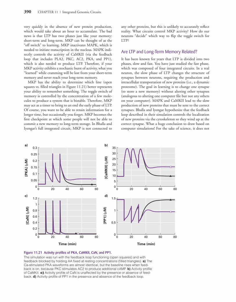
390 CHAPTER 11 | Integrated Genomic Circuits
d)
b)
c)
a)
040200 60 80
0.4
0.2
0.8
1
0.6
[Ca
N]
(µM
)
1.2
Time (min)
040200 60 80
0.5
1
[PP
1]
(µM
)
1.5
040200 60 80
10
5
20
25
30
15
[Ca
MK
II]
(µM
)
35
040200 60 80
0.1
0.05
0.15
0.2
0.25
[PK
A]
(µM
)
0.3
Time (min)
Figure 11.21 Activity profiles of PKA, CaMKII, CaN, and PP1.The simulation was run with the feedback loop functioning (open squares) and withfeedback blocked by holding AA fixed at resting concentrations (filled triangles). a) TheCa-stimulated PKA waveforms are almost identical, but the baseline rises when feed-back is on, because PKC stimulates AC2 to produce additional cAMP. b) Activity profileof CaMKII. c) Activity profile of CaN is unaffected by the presence or absence of feed-back. d) Activity profile of PP1 in the presence and absence of the feedback loop.
very quickly in the absence of new protein production,which would take about an hour to accumulate. The badnews is that LTP has two phases just like your memory:short-term and long-term. MKP can be thought of as the“off switch” to learning. MKP inactivates MAPK, which isneeded to initiate transcription in the nucleus. MAPK indi-rectly controls the activity of CaMKII (via the feedbackloop that includes PLA2, PKC, AC2, PKA, and PP1),which is also needed to produce LTP. Therefore, if yourMKP activity exhibits a stochastic burst of activity, what you“learned” while cramming will be lost from your short-termmemory and never reach your long-term memory.
MKP has the ability to determine which line (opensquares vs. filled triangles in Figure 11.21) better representsyour ability to remember something. The toggle switch ofmemory is controlled by the concentration of a few mole-cules to produce a system that is bistable. Therefore, MKPmay act as a timer to bring to an end the early phase of LTP.Of course, you want to be able to retain information for alonger time, but occasionally you forget. MKP becomes thefirst checkpoint at which some people will not be able tocommit a new memory to long-term storage. In Bhalla andIyengar’s full integrated circuit, MKP is not connected to
any other proteins, but this is unlikely to accurately reflectreality. What circuits control MKP activity? How do ourneurons “decide” which way to flip the toggle switch forLTP?
Are LTP and Long-Term Memory Related?
It has been known for years that LTP is divided into twophases, slow and fast. You have just studied the fast phase,which was composed of four integrated circuits. In a realneuron, the slow phase of LTP changes the structure ofsynapses between neurons, requiring the production andintracellular transportation of new proteins (i.e., a dynamicproteome). The goal in learning is to change one synapse(to store a new memory) without altering other synapses(analogous to altering one computer file but not any otherson your computer). MAPK and CaMKII lead to the slowproduction of new proteins that must be sent to the correctsynapses. Bhalla and Iyengar hypothesize that the feedbackloop described in their simulation controls the localizationof new proteins via the cytoskeleton so they wind up at thecorrect synapse. What a huge conclusion to draw based oncomputer simulations! For the sake of science, it does not
CAMPMC11_0805382194.QXD 6/12/06 11:56 AM Page 390
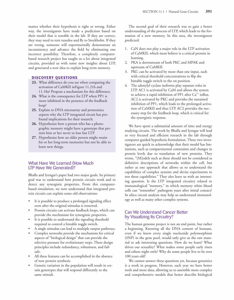
SECTION 11.1 | Natural Gene Circuits 391
matter whether their hypothesis is right or wrong. Eitherway, the investigators have made a prediction based ontheir model that is testable in the lab. If they are correct,they may need to rent tuxedos and fly to Stockholm. If theyare wrong, someone will experimentally demonstrate aninconsistency and advance the field by eliminating oneincorrect possibility. Therefore, a completely computer-based research project has taught us a lot about integratedcircuits, provided us with some new insights about LTP,and generated a new idea to explain long-term memory.
DISCOVE RY QU ESTIONS23. What difference do you see when comparing the
activation of CaMKII inFigure 11.21b and11.18a? Propose a mechanism for this difference.
24. What is the consequence for LTP when PP1 ismore inhibited in the presence of the feedbackloop?
25. Explain to DNA microarray and proteomicsexperts why the LTP integrated circuit has pro-found implications for their research.
26. Hypothesize how a person who has a photo-graphic memory might have a genotype that per-mits him or her never to lose fast LTP.
27. Hypothesize how an older person might retainhis or her long-term memories but not be able tolearn new things.
What Have We Learned (How Much LTP Have We Generated)?
Bhalla and Iyengar’s paper had two major goals. Its primarygoal was to understand how protein circuits work and todetect any synergistic properties. From this computer-based simulation, we now understand that integrated pro-tein circuits can explain some old observations:
• It is possible to produce a prolonged signaling effecteven after the original stimulus is removed.
• Protein circuits can activate feedback loops, which canprovide the mechanism for synergistic properties.
• It is possible to understand the signaling thresholdrequired to control a bistable toggle switch.
• A single stimulus can lead to multiple output pathways.• Complex networks provide the mechanism for critical
aspects of “biological design” that can provide theselective pressure for evolutionary steps. These designprinciples include redundancy, robustness, and fail-safe.
• All these features can be accomplished in the absenceof new protein synthesis.
• Genetic variation in the population will result in cer-tain genotypes that will respond differently to thesame stimuli.
The second goal of their research was to gain a betterunderstanding of the process of LTP, which leads to the for-mation of a new memory. In this area, the investigatorspredicted:
1. CaN does not play a major role in the LTP activationof CaMKII, which most believe is a critical protein inlearning.
2. PKA is downstream of both PKC and MPAK andupstream of CaMKII.
3. PKC can be activated by more than one input, eachwith critical threshold concentrations to flip thebistable toggle switch to the on position.
4. The adenylyl cyclase isoforms play separate roles inLTP. AC1 is activated by CaM and allows the systemto achieve a rapid inhibition of PP1 after Ca2+ influx.AC2 is activated by PKC and provides the sustainedinhibition of PP1, which leads to the prolonged activa-tion of CaMKII and thus LTP. AC2 provides the nec-essary step for the feedback loop, which is critical forthe synergistic response.
We have spent a substantial amount of time and energystudying circuits. The work by Bhalla and Iyengar will leadto very focused and efficient research in the lab throughcomputer-guided hypothesis formulation. These two inves-tigators are quick to acknowledge that their model has lim-itations, such as compartmental constraints and changes inprotein levels due to translation of new proteins. Theywrote, “[M]odels such as these should not be considered asdefinitive descriptions of networks within the cell, butrather as one approach that allows us to understand thecapabilities of complex systems and devise experiments totest these capabilities.” They also leave us with an interest-ing question. Is the LTP integrated circuitry related toimmunological “memory,” in which memory white bloodcells can “remember” pathogens years after initial contact?In silico circuit analysis may help us understand immunol-ogy as well as many other complex systems.
Can We Understand Cancer Better by Visualizing Its Circuitry?
The human genome project is not an end point, but rathera beginning. Knowing all the DNA content of humans,even if we knew every single nucleotide polymorphism(SNP) in the gene pool, would only give us the raw mate-rial to ask interesting questions. How do we learn? Whatdrives our sexuality? What makes some people early risersand others night owls? Why do some people live to be over100 years old?
We cannot answer these questions yet, because genomicsis a work in progress. However, each year we have bettertools and more data, allowing us to assemble more complexand comprehensive models that better describe biological
CAMPMC11_0805382194.QXD 6/12/06 11:56 AM Page 391
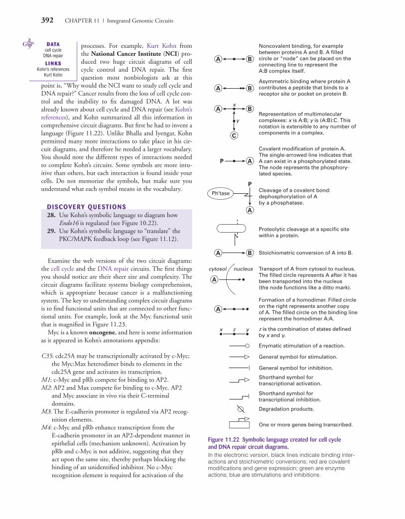
392 CHAPTER 11 | Integrated Genomic Circuits
A B
A B
C
A B
A
A B
A
P
P
A
x
z yx
cytosol nucleus
y
A
Ph’tase
Noncovalent binding, for examplebetween proteins A and B. A filledcircle or “node” can be placed on theconnecting line to represent theA:B complex itself.
Asymmetric binding where protein Acontributes a peptide that binds to areceptor site or pocket on protein B.
Representation of multimolecularcomplexes: x is A:B; y is (A:B):C. Thisnotation is extensible to any number ofcomponents in a complex.
Covalent modification of protein A.The single-arrowed line indicates thatA can exist in a phosphorylated state.The node represents the phosphory-lated species.
Cleavage of a covalent bond:dephosphorylation of Aby a phosphatase.
Proteolytic cleavage at a specific sitewithin a protein.
Transport of A from cytosol to nucleus.The filled circle represents A after it hasbeen transported into the nucleus(the node functions like a ditto mark).
Formation of a homodimer. Filled circleon the right represents another copyof A. The filled circle on the binding linerepresent the homodimer A:A.
z is the combination of states definedby x and y.
One or more genes being transcribed.
Degradation products.
Shorthand symbol fortranscriptional inhibition.
Shorthand symbol fortranscriptional activation.
General symbol for inhibition.
General symbol for stimulation.
Enymatic stimulation of a reaction.
Stoichiometric conversion of A into B.
Figure 11.22 Symbolic language created for cell cycleand DNA repair circuit diagrams. In the electronic version, black lines indicate binding inter-actions and stoichiometric conversions; red are covalentmodifications and gene expression; green are enzymeactions; blue are stimulations and inhibitions.
processes. For example, Kurt Kohn fromthe National Cancer Institute (NCI) pro-duced two huge circuit diagrams of cellcycle control and DNA repair. The firstquestion most nonbiologists ask at this
point is, “Why would the NCI want to study cell cycle andDNA repair?” Cancer results from the loss of cell cycle con-trol and the inability to fix damaged DNA. A lot wasalready known about cell cycle and DNA repair (see Kohn’sreferences), and Kohn summarized all this information incomprehensive circuit diagrams. But first he had to invent alanguage (Figure 11.22). Unlike Bhalla and Iyengar, Kohnpermitted many more interactions to take place in his cir-cuit diagrams, and therefore he needed a larger vocabulary.You should note the different types of interactions neededto complete Kohn’s circuits. Some symbols are more intu-itive than others, but each interaction is found inside yourcells. Do not memorize the symbols, but make sure youunderstand what each symbol means in the vocabulary.
DISCOVE RY QU ESTIONS28. Use Kohn’s symbolic language to diagram how
Endo16 is regulated (see Figure 10.22).29. Use Kohn’s symbolic language to “translate” the
PKC/MAPK feedback loop (see Figure 11.12).
Examine the web versions of the two circuit diagrams:the cell cycle and the DNA repair circuits. The first thingsyou should notice are their sheer size and complexity. Thecircuit diagrams facilitate systems biology comprehension,which is appropriate because cancer is a malfunctioningsystem. The key to understanding complex circuit diagramsis to find functional units that are connected to other func-tional units. For example, look at the Myc functional unitthat is magnified in Figure 11.23.
Myc is a known oncogene, and here is some informationas it appeared in Kohn’s annotations appendix:
C35: cdc25A may be transcriptionally activated by c-Myc;the Myc:Max heterodimer binds to elements in thecdc25A gene and activates its transcription.
M1: c-Myc and pRb compete for binding to AP2.M2: AP2 and Max compete for binding to c-Myc. AP2
and Myc associate in vivo via their C-terminaldomains.
M3: The E-cadherin promoter is regulated via AP2 recog-nition elements.
M4: c-Myc and pRb enhance transcription from the E-cadherin promoter in an AP2-dependent manner inepithelial cells (mechanism unknown). Activation bypRb and c-Myc is not additive, suggesting that theyact upon the same site, thereby perhaps blocking thebinding of an unidentified inhibitor. No c-Myc recognition element is required for activation of the
DATAcell cycle
DNA repair
L I N KSKohn’s references
Kurt Kohn
CAMPMC11_0805382194.QXD 6/12/06 11:56 AM Page 392

SECTION 11.1 | Natural Gene Circuits 393
Myc boxpRb
AP2
Maxc-Myc
E-cadherin
cdc25A C35
M2
M1
M4
M3
Figure 11.23 Myc subsection from Kohn’s cell cycle circuit.The Myc box can be found in area D10, in the top right cor-ner of the DNA repair circuit diagram. Symbols are definedin Figure 11.22.
E-cadherin promoter by c-Myc. Max blocks transcriptional activation from the E-cadherin pro-moter by c-Myc, presumably because it blocks thebinding between c-Myc and AP2.
The proteins retinoblastoma (pRb, a tumor suppressor)and c-Myc compete to bind to the transcription factor AP2.The two possible combinations c-Myc/Max and pRb/AP2can each bind to cis-regulatory elements to initiate tran-scription of E-cadherin. However, c-Myc can also bind toMax and lead to the transcription of cdc25A, a phosphatasethat regulates the activity of a number of proteins in otherfunctional domains. However, note that regulation of c-Mycin this functional unit is influenced by a different functionalunit, as indicated by the arrow to the left of c-Myc.
From our examination of learning circuits, we know thatfeedback loops are very important. Let’s look at one feed-back loop in each of these circuit diagrams. Open the cellcycle file to locate cdc25C and cycB:cdk1 (in area H4).
1. cdc25C is activated by phosphorylation (blue line withgreen C18 label).
2. cdc25C removes phosphates from cdk1 at amino acidsT14 and Y15 (shown as a green line coming fromcdc25C). Removal of the phosphates removes the inhi-bition from cdk1.
3. cdk1 interacts with cycA (black C5 label), and thisinteraction stimulates the phosphorylation of cdc25C(green C36). Although this positive feedback loop isdifficult to recognize at first glance, with practice andfamiliarity with the system, you would be able to seeother examples.
The second feedback loop is taken from the DNA repairdiagram. Locate p53 in area E7–9 on the right side of the
circuit. Immediately you can tell that p53 is a critical compo-nent, because there are so many interactions emanating fromit. If you look below p53, you will see three black dots (blackP18), which indicates that p53 (the protein) can formhomotetramers. The homotetramer can initiate transcription(black P17) from seven different genes (one box with sevenred lines emanating from it). One of the activated genes isMdm2 (red P39), and the protein MDM2 can form a het-erodimer with p53 (black P28), which inhibits transcriptionof the Mdm2 gene (blue P29). These components form anegative feedback loop. In the published paper accompany-ing this circuit diagram, Kohn reported that MDM2/p53formation leads to the degradation of p53 (black P30), asindicated by the blue arrow labeled P31.
All these interactions were discernible from circuit dia-grams with very few words, and they allow us to compre-hend interactions and make predictions. Kohn’s circuitdiagrams are works in progress; don’t make the mistake ofassuming that if a component is shown in the diagram, allof its interactions are known. Our knowledge is limited,and studying circuit diagrams will focus our research moreefficiently. We are beginning to make headway on larger-scale models, but we still have a lot to learn.
DISCOVE RY QU ESTIONS30. In Kohn’s circuit diagrams, try to locate one small
functional subcircuit (similar to the Myc subcir-cuit), and describe in words what you see. Whichcomponents are linked to other functional units?
31. Find BRCA1, the breast cancer gene, located inarea F10 of the DNA repair circuit. Describe inwords how BRCA1 interacts with p53.
32. One of the blue lines below p53 is labeled P31.Notice that two different repressors can block thedegradation of p53. Given what you know aboutcircuits, is blocking this degradation an impor-tant process or not? What effect would tworepressive interactions have on the reliability ofblocking the degradation of p53? Can you findany other pathways that also block the degrada-tion of p53?
33. If you became fluent in this symbolic language,do you think you should get a foreign languagecredit?
Summary 11.1We have seen that genetic toggle switches can be formedwith very few genes. Genomes contain hundreds or thou-sands of toggle switches so they can produce proteomes andmetabolomes in response to environmental changes. The“choice” between two responses can be driven by particularfactors (e.g., nutrient concentration for λ phage lysogenic
CAMPMC11_0805382194.QXD 6/12/06 11:56 AM Page 393

394 CHAPTER 11 | Integrated Genomic Circuits
promoter repressor GFPpromoterrepressor
Inducer
Inducer
Figure 11.24 Theoretical two-gene bistable toggle switch.The black gene “repressor” is transcribed from its black promoter. The black repressorprotein binds to the gray promoter to block the production of the gray repressor protein.The gray repressor protein blocks the production of the black repressor protein whenthe gray repressor protein binds to the black promoter. To detect which state the toggleswitch is in, GFP was placed downstream of the gray promoter so that the gray repres-sor and GFP are produced simultaneously.
versus lytic lifestyles) or by stochastic behaviorof proteins (e.g., recA and lacZ promoters).Given our understanding of how bistablegenetic switches operate, can we design and
construct synthetic bistable toggle switches that function aspredicted? If so, could these synthetic switches be used toproduce useful devices? If you were designing a bistableswitch for gene therapy, you would want to incorporate alevel of redundancy that provided the patient with anacceptable degree of reliability. It might seem uncomfort-able to treat genes like machines with reliability that can becalculated, but this approach to genome analysis is valu-able. Applying engineering principles to genomics helps usunderstand why diploids evolved the apparent waste incomplex circuits with redundancies. In Section 11.2, westudy a series of synthetic genomic circuits that illustratethe cutting edge of our knowledge of how biological cir-cuits work.
11.2 Synthetic BiologyEvery time we build a model, we are trying to create a sim-ple version of a complex system. Given the lessons in Sec-tion 11.1, is it possible to design and construct syntheticcircuits? The new field of synthetic biology (analogous tosynthetic chemistry) applies engineering principles togenomic circuits to construct small biological devices thatshould help us understand how naturally evolved circuitsfunction. Perhaps someday we will be able to construct syn-thetic circuits that can perform beneficial tasks, but for theforeseeable future, we will use synthetic components,devices, and systems to elucidate how natural circuits func-tion. In this section, we will consider four case studies thatincrease in complexity. Use these examples as starting placesfor synthetic circuits you might want to construct and test.Discovery Questions will allow you to explore the field of
synthetic biology, including an interactive constructionweb site which is part of the BioBricks project at theMassachusetts Institute of Technology (MIT).
Can Humans Engineer a Genetic Toggle Switch?
Often there is a division among biologists who like to argueabout which experiments are “real science”: those workingwith naturally produced organisms and molecules vs. thoseworking with theoretical models to unify experimentalobservations. Both approaches are necessary for a completeunderstanding, but it is important to remember that pre-dictions based on theoretical models must be tested withreal experiments. In 2000, two research groups describedgenetic toggle switches that had been design and con-structed. Both groups used E. coli as the host for theirswitches, but they made two different types of switches.One group built a toggle switch very similar to the oneused by λ phage to choose its lifestyle. We’ll examine thisswitch first. Later we examine a switch that oscillates like acircadian clock.
How to Build a Toggle Switch
Timothy Gardner and his colleagues Jim Collins andCharles Cantor at Boston University built a toggle switchthat could choose between two states. However, rather thanletting E. coli determine which direction to go, they con-structed a toggle switch that could be regulated by theinvestigators (Figure 11.24). In this switch, they neededtwo constitutive promoters (colored black and gray) andtwo repressor genes (also colored black and gray). Theblack repressor protein silences the gray promoter, whichdrives production of the gray repressor protein. Conversely,the gray repressor protein silences the black promoter,which drives production of the black repressor protein.
L I N KSJim Collins
Charles CantorTimothy Gardner
CAMPMC11_0805382194.QXD 6/12/06 11:56 AM Page 394
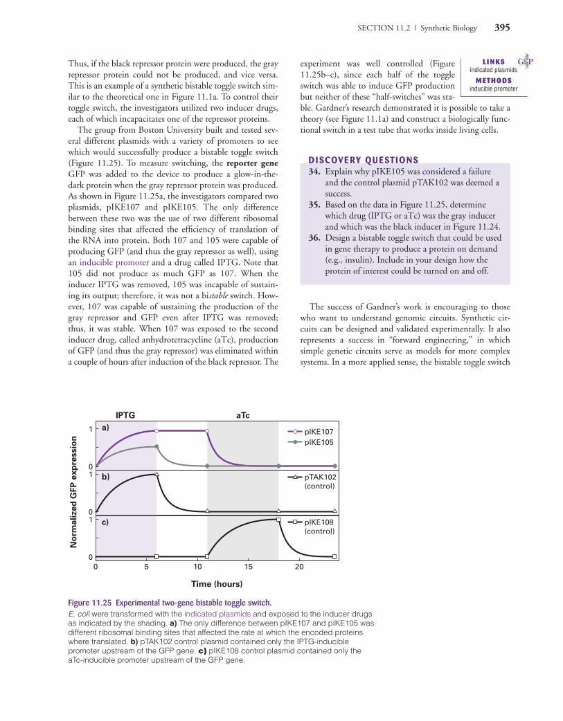
SECTION 11.2 | Synthetic Biology 395
aTcIPTG
0 5 10 15 200
10
10
1
Time (hours)
No
rma
lize
d G
FP
ex
pre
ssio
n
pIKE107pIKE105
pTAK102(control)
pIKE108(control)
a)
b)
c)
Figure 11.25 Experimental two-gene bistable toggle switch.E. coli were transformed with the indicated plasmids and exposed to the inducer drugsas indicated by the shading. a) The only difference between pIKE107 and pIKE105 wasdifferent ribosomal binding sites that affected the rate at which the encoded proteinswhere translated. b) pTAK102 control plasmid contained only the IPTG-inducible promoter upstream of the GFP gene. c) pIKE108 control plasmid contained only theaTc-inducible promoter upstream of the GFP gene.
Thus, if the black repressor protein were produced, the grayrepressor protein could not be produced, and vice versa.This is an example of a synthetic bistable toggle switch sim-ilar to the theoretical one in Figure 11.1a. To control theirtoggle switch, the investigators utilized two inducer drugs,each of which incapacitates one of the repressor proteins.
The group from Boston University built and tested sev-eral different plasmids with a variety of promoters to seewhich would successfully produce a bistable toggle switch(Figure 11.25). To measure switching, the reporter geneGFP was added to the device to produce a glow-in-the-dark protein when the gray repressor protein was produced.As shown in Figure 11.25a, the investigators compared twoplasmids, pIKE107 and pIKE105. The only differencebetween these two was the use of two different ribosomalbinding sites that affected the efficiency of translation ofthe RNA into protein. Both 107 and 105 were capable ofproducing GFP (and thus the gray repressor as well), usingan inducible promoter and a drug called IPTG. Note that105 did not produce as much GFP as 107. When theinducer IPTG was removed, 105 was incapable of sustain-ing its output; therefore, it was not a bistable switch. How-ever, 107 was capable of sustaining the production of thegray repressor and GFP even after IPTG was removed;thus, it was stable. When 107 was exposed to the secondinducer drug, called anhydrotetracycline (aTc), productionof GFP (and thus the gray repressor) was eliminated withina couple of hours after induction of the black repressor. The
experiment was well controlled (Figure11.25b–c), since each half of the toggleswitch was able to induce GFP productionbut neither of these “half-switches” was sta-ble. Gardner’s research demonstrated it is possible to take atheory (see Figure 11.1a) and construct a biologically func-tional switch in a test tube that works inside living cells.
DISCOVE RY QU ESTIONS34. Explain why pIKE105 was considered a failure
and the control plasmid pTAK102 was deemed asuccess.
35. Based on the data in Figure 11.25, determinewhich drug (IPTG or aTc) was the gray inducerand which was the black inducer in Figure 11.24.
36. Design a bistable toggle switch that could be usedin gene therapy to produce a protein on demand(e.g., insulin). Include in your design how theprotein of interest could be turned on and off.
The success of Gardner’s work is encouraging to thosewho want to understand genomic circuits. Synthetic cir-cuits can be designed and validated experimentally. It alsorepresents a success in “forward engineering,” in whichsimple genetic circuits serve as models for more complexsystems. In a more applied sense, the bistable toggle switch
L I N KSindicated plasmids
M ETHODSinducible promoter
CAMPMC11_0805382194.QXD 6/12/06 11:56 AM Page 395
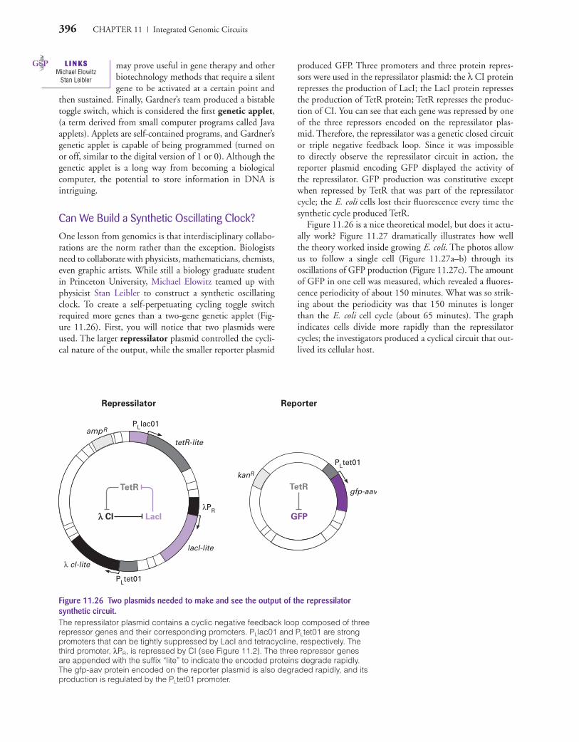
396 CHAPTER 11 | Integrated Genomic Circuits
TetR
LacI
Repressilator Reporter
λ λ Cl
TetR
GFP
PLlac01
PLtet01
λPR
tetR-lite
gfp-aav
kanR
ampR
lacI-lite
λ cI-lite
PLtet01
Figure 11.26 Two plasmids needed to make and see the output of the repressilator synthetic circuit.The repressilator plasmid contains a cyclic negative feedback loop composed of threerepressor genes and their corresponding promoters. PLlac01 and PLtet01 are strong promoters that can be tightly suppressed by LacI and tetracycline, respectively. Thethird promoter, λPR, is repressed by CI (see Figure 11.2). The three repressor genes are appended with the suffix “lite” to indicate the encoded proteins degrade rapidly. The gfp-aav protein encoded on the reporter plasmid is also degraded rapidly, and itsproduction is regulated by the PLtet01 promoter.
may prove useful in gene therapy and otherbiotechnology methods that require a silentgene to be activated at a certain point and
then sustained. Finally, Gardner’s team produced a bistabletoggle switch, which is considered the first genetic applet,(a term derived from small computer programs called Javaapplets). Applets are self-contained programs, and Gardner’sgenetic applet is capable of being programmed (turned onor off, similar to the digital version of 1 or 0). Although thegenetic applet is a long way from becoming a biologicalcomputer, the potential to store information in DNA isintriguing.
Can We Build a Synthetic Oscillating Clock?
One lesson from genomics is that interdisciplinary collabo-rations are the norm rather than the exception. Biologistsneed to collaborate with physicists, mathematicians, chemists,even graphic artists. While still a biology graduate studentin Princeton University, Michael Elowitz teamed up withphysicist Stan Leibler to construct a synthetic oscillatingclock. To create a self-perpetuating cycling toggle switchrequired more genes than a two-gene genetic applet (Fig-ure 11.26). First, you will notice that two plasmids wereused. The larger repressilator plasmid controlled the cycli-cal nature of the output, while the smaller reporter plasmid
produced GFP. Three promoters and three protein repres-sors were used in the repressilator plasmid: the λ CI proteinrepresses the production of LacI; the LacI protein repressesthe production of TetR protein; TetR represses the produc-tion of CI. You can see that each gene was repressed by oneof the three repressors encoded on the repressilator plas-mid. Therefore, the repressilator was a genetic closed circuitor triple negative feedback loop. Since it was impossibleto directly observe the repressilator circuit in action, thereporter plasmid encoding GFP displayed the activity ofthe repressilator. GFP production was constitutive exceptwhen repressed by TetR that was part of the repressilatorcycle; the E. coli cells lost their fluorescence every time thesynthetic cycle produced TetR.
Figure 11.26 is a nice theoretical model, but does it actu-ally work? Figure 11.27 dramatically illustrates how wellthe theory worked inside growing E. coli. The photos allowus to follow a single cell (Figure 11.27a–b) through itsoscillations of GFP production (Figure 11.27c). The amountof GFP in one cell was measured, which revealed a fluores-cence periodicity of about 150 minutes. What was so strik-ing about the periodicity was that 150 minutes is longerthan the E. coli cell cycle (about 65 minutes). The graphindicates cells divide more rapidly than the repressilatorcycles; the investigators produced a cyclical circuit that out-lived its cellular host.
L I N KSMichael Elowitz
Stan Leibler
CAMPMC11_0805382194.QXD 6/12/06 11:56 AM Page 396

SECTION 11.2 | Synthetic Biology 397
0
20
Time (min)
0 100 200 300
Flu
ore
scen
ce
(arb
irta
ry u
nit
s)
400 500 600
40
60
80
100
120
Time (min)
60 250140 300 390 450 550 600
c)
b)
a)
Figure 11.27 Cyclical toggle switching in live bacteria.a) Fluorescence and b) phase contrast microscopy images of cells, revealing the timecourse of GFP expression and cell growth beginning with a single bacterium containingthe repressilator and reporter plasmids (see Figure 11.26). Scale bar in b) indicates 4 µm in the photographs. c) The pictures in a) and b) correspond to peaks and troughsin the time course of GFP fluorescence intensity of the selected cell. Bars at the bottomof panel c) indicate the timing of cell division, as estimated from the phase contrast photomicrographs in panel b).
Math Minute 11.3 How Can You Visualize Gene Regulation Logic?
The schematic representation of the repressilator (Figure 11.26) contains informationabout how the device was constructed and how it works. However, schematic represen-tations require you to follow the logic in your head to understand the behavior of thesystem. In this Math Minute, we explore how two other representations, truth tablesand logic gates, are used to summarize gene regulation logic and behavior of systemslike the repressilator.
Truth tables and logic gates describe a system of binary variables, each of which hasthe value 0 or 1. Gene regulation can be modeled with a binary system by representinggene expression as either “on” (= 1) or “off ” (= 0) and regulatory elements as either“present” (= 1) or “absent” (= 0). For example, the simple binary function AND, whichhas the value 0 unless both input variables have the value 1, was used in statement 2 ofTable 10.3 to model the toggle between control by module A and module B. The logicgate and truth table for the AND function are shown in Figure MM11.3a. The purposeof a truth table is to list the value of output variables for each possible combination ofinput variable values. A logic gate is a standardized symbol that encapsulates the sameinformation for elementary functions; some of the most common logic gates and thecorresponding truth tables are shown in Figure MM11.3.
CAMPMC11_0805382194.QXD 6/12/06 11:56 AM Page 397
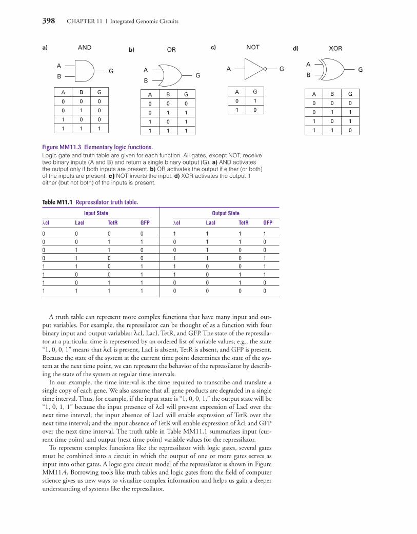
398 CHAPTER 11 | Integrated Genomic Circuits
a) AND
A
0
0
1
1 1 1
0
0
0
0
1
0
B G
A
BG
c) NOT
A
0
1 0
1
G
GA
b) OR
A
0
0
1
1 1 1
1
1
0
0
1
0
B G
A
BG
d) XOR
A
0
0
1
1 1 0
1
1
0
0
1
0
B G
A
BG
Figure MM11.3 Elementary logic functions.Logic gate and truth table are given for each function. All gates, except NOT, receivetwo binary inputs (A and B) and return a single binary output (G). a) AND activatesthe output only if both inputs are present. b) OR activates the output if either (or both)of the inputs are present. c) NOT inverts the input. d) XOR activates the output ifeither (but not both) of the inputs is present.
A truth table can represent more complex functions that have many input and out-put variables. For example, the repressilator can be thought of as a function with fourbinary input and output variables: λcI, LacI, TetR, and GFP. The state of the repressila-tor at a particular time is represented by an ordered list of variable values; e.g., the state“1, 0, 0, 1” means that λcI is present, LacI is absent, TetR is absent, and GFP is present.Because the state of the system at the current time point determines the state of the sys-tem at the next time point, we can represent the behavior of the repressilator by describ-ing the state of the system at regular time intervals.
In our example, the time interval is the time required to transcribe and translate asingle copy of each gene. We also assume that all gene products are degraded in a singletime interval. Thus, for example, if the input state is “1, 0, 0, 1,” the output state will be“1, 0, 1, 1” because the input presence of λcI will prevent expression of LacI over thenext time interval; the input absence of LacI will enable expression of TetR over thenext time interval; and the input absence of TetR will enable expression of λcI and GFPover the next time interval. The truth table in Table MM11.1 summarizes input (cur-rent time point) and output (next time point) variable values for the repressilator.
To represent complex functions like the repressilator with logic gates, several gatesmust be combined into a circuit in which the output of one or more gates serves asinput into other gates. A logic gate circuit model of the repressilator is shown in FigureMM11.4. Borrowing tools like truth tables and logic gates from the field of computerscience gives us new ways to visualize complex information and helps us gain a deeperunderstanding of systems like the repressilator.
Table M11.1 Repressilator truth table.
Input State Output State
λcI LacI TetR GFP λcI LacI TetR GFP
0 0 0 0 1 1 1 10 0 1 1 0 1 1 00 1 1 0 0 1 0 00 1 0 0 1 1 0 11 1 0 1 1 0 0 11 0 0 1 1 0 1 11 0 1 1 0 0 1 01 1 1 1 0 0 0 0
CAMPMC11_0805382194.QXD 6/12/06 11:56 AM Page 398

SECTION 11.2 | Synthetic Biology 399
TTetR
Lacl
λcl
GFP
input output
Tinput output
Tinput output
Tinput output
Figure MM11.4 Logic gate circuit model of repressilator.The time interval for propagating values from one variable toanother is represented by the “T” in each NOT gate. The inputstate of the system is indicated by the labeled arrows to theleft of each NOT gate. The output state of the system is indi-cated by the labeled arrows to the right of each NOT gate.
MATH M I N UTE D ISCOVE RY QU ESTION1. Why doesn’t the repressilator get locked into a cycle of alternating between all
0’s and all 1’s?
The very regular periodicity of the repressilator helpsyou appreciate your own circadian rhythm and how it toocan be controlled by a small number of genes that producecyclical amounts of protein. However, there is a fly in thisointment of perfect timing. Noise and stochastic behaviorof proteins are a fundamental property of gene regulationand protein production, so you might expect some prob-lems with the regularity of the repressilator.
DISCOVE RY QU ESTIONS37. How can a biological clock outlive its host cell?38. Graph the production of CI, LacI, and TetR
proteins on top of the graph in Figure 11.27c.
39. Why did the investigators choose proteins thatare rapidly degraded by cells? What would havehappened if the proteins were long-lived?
40. Predict what might happen to the repressilatorperiodicity inside sister cells after division.
41. What would be required for sister cells to main-tain the exact same periodicity of GFP produc-tion? In other words, does the repressilator haveany means for cooperation through communica-tion or checkpoints (see pages 376)?
Given the clarity of the data in Figure 11.27c, you mightthink humans can construct a clock that is unaffected by
CAMPMC11_0805382194.QXD 6/12/06 11:56 AM Page 399
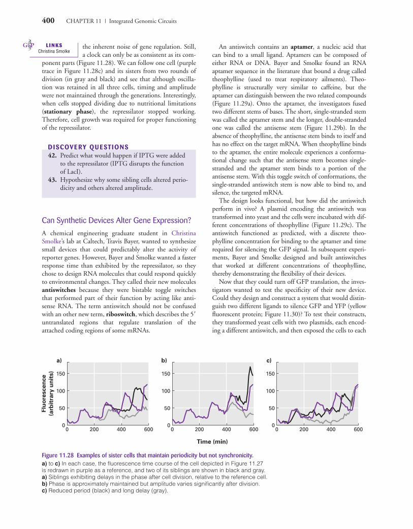
400 CHAPTER 11 | Integrated Genomic Circuits
Flu
ore
scen
ce
(arb
itra
ry u
nit
s)
a)
400
Time (min)
b) c)
0
50
0 200 400 600
100
150
0
50
0 200 600
100
150
0
50
0 200 400 600
100
150
Figure 11.28 Examples of sister cells that maintain periodicity but not synchronicity.a) to c) In each case, the fluorescence time course of the cell depicted in Figure 11.27is redrawn in purple as a reference, and two of its siblings are shown in black and gray.a) Siblings exhibiting delays in the phase after cell division, relative to the reference cell.b) Phase is approximately maintained but amplitude varies significantly after division. c) Reduced period (black) and long delay (gray).
the inherent noise of gene regulation. Still,a clock can only be as consistent as its com-
ponent parts (Figure 11.28). We can follow one cell (purpletrace in Figure 11.28c) and its sisters from two rounds ofdivision (in gray and black) and see that although oscilla-tion was retained in all three cells, timing and amplitudewere not maintained through the generations. Interestingly,when cells stopped dividing due to nutritional limitations(stationary phase), the repressilator stopped working.Therefore, cell growth was required for proper functioningof the repressilator.
DISCOVE RY QU ESTIONS42. Predict what would happen if IPTG were added
to the repressilator (IPTG disrupts the functionof LacI).
43. Hypothesize why some sibling cells altered perio-dicity and others altered amplitude.
Can Synthetic Devices Alter Gene Expression?
A chemical engineering graduate student in ChristinaSmolke’s lab at Caltech, Travis Bayer, wanted to synthesizesmall devices that could predictably alter the activity ofreporter genes. However, Bayer and Smolke wanted a fasterresponse time than exhibited by the repressilator, so theychose to design RNA molecules that could respond quicklyto environmental changes. They called their new moleculesantiswitches because they were bistable toggle switchesthat performed part of their function by acting like anti-sense RNA. The term antiswitch should not be confusedwith an other new term, riboswitch, which describes the 5�untranslated regions that regulate translation of theattached coding regions of some mRNAs.
An antiswitch contains an aptamer, a nucleic acid thatcan bind to a small ligand. Aptamers can be composed ofeither RNA or DNA. Bayer and Smolke found an RNAaptamer sequence in the literature that bound a drug calledtheophylline (used to treat respiratory ailments). Theo-phylline is structurally very similar to caffeine, but theaptamer can distinguish between the two related compounds(Figure 11.29a). Onto the aptamer, the investigators fusedtwo different stems of bases. The short, single-stranded stemwas called the aptamer stem and the longer, double-strandedone was called the antisense stem (Figure 11.29b). In theabsence of theophylline, the antisense stem binds to itself andhas no effect on the target mRNA. When theophylline bindsto the aptamer, the entire molecule experiences a conforma-tional change such that the antisense stem becomes single-stranded and the aptamer stem binds to a portion of theantisense stem. With this toggle switch of conformations, thesingle-stranded antiswitch stem is now able to bind to, andsilence, the targeted mRNA.
The design looks functional, but how did the antiswitchperform in vivo? A plasmid encoding the antiswitch wastransformed into yeast and the cells were incubated with dif-ferent concentrations of theophylline (Figure 11.29c). Theantiswitch functioned as predicted, with a discrete theo-phylline concentration for binding to the aptamer and timerequired for silencing the GFP signal. In subsequent experi-ments, Bayer and Smolke designed and built antiswitchesthat worked at different concentrations of theophylline,thereby demonstrating the flexibility of their devices.
Now that they could turn off GFP translation, the inves-tigators wanted to test the specificity of their new device.Could they design and construct a system that would distin-guish two different ligands to silence GFP and YFP (yellowfluorescent protein; Figure 11.30)? To test their constructs,they transformed yeast cells with two plasmids, each encod-ing a different antiswitch, and then exposed the cells to each
L I N KSChristina Smolke
CAMPMC11_0805382194.QXD 6/12/06 11:56 AM Page 400
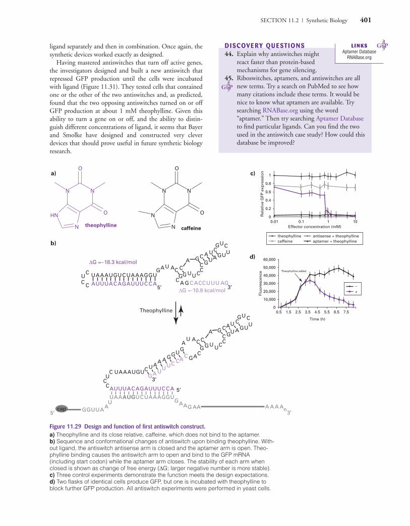
SECTION 11.2 | Synthetic Biology 401
a)
b)
c)
d)
O
O
theophyllinecaffeine
N N
N
HN
O
O
N N
N
N0.01 0.1 1 10
0.2
0
00.5 1.5 2.5 3.5 4.5
Time (h)
5.5 6.5 7.5
10,000
20,000
30,000
40,000
50,000
60,000
0.4
0.6
0.8
1
Rel
ativ
e G
FP e
xpre
ssio
nFl
uo
resc
ence
Effector concentration (mM)
Theophylline added
∆G =−18.3 kcal/mol
∆G =-10.8 kcal/mol
UC
C
C U
A
A
U
A
U
A
U
U
A
G
C
U
A
C
G
U
A
A
U
A
U
A
U
G
C
G
C
U
A
U
UU
UUU
UU
G
GG
G
G
GG
5’
5’
5’
3’
3’
3’
C
C
C CC
CC
CC
AA
A A A
AAAAA
A
AAAA
A A
AA
A AA
A
A A
UU
U
UU
U G G
A A An
G GC CCUUU
AA
A
Theophylline
U
A
AA
U
U
U
U
UUU
U
UU
UU
U
U
UU
A
U
A
A
U
C
G
GG
A
U
G
G
G
G
GG GG
GG
G
G
G
C
CC
C
CC
C
C
CC
C
CC
C
C
C
CA
U
U
A
U
A
U
A
C
G
C
G
A
U
cap
–+
theophyllinecaffeine
antisense + theophyllineaptamer + theophylline
Figure 11.29 Design and function of first antiswitch construct.a) Theophylline and its close relative, caffeine, which does not bind to the aptamer. b) Sequence and conformational changes of antiswitch upon binding theophylline. With-out ligand, the antiswitch antisense arm is closed and the aptamer arm is open. Theo-phylline binding causes the antiswitch arm to open and bind to the GFP mRNA(including start codon) while the aptamer arm closes. The stability of each arm whenclosed is shown as change of free energy (∆G; larger negative number is more stable).c) Three control experiments demonstrate the function meets the design expectations.d) Two flasks of identical cells produce GFP, but one is incubated with theophylline toblock further GFP production. All antiswitch experiments were performed in yeast cells.
ligand separately and then in combination. Once again, thesynthetic devices worked exactly as designed.
Having mastered antiswitches that turn off active genes,the investigators designed and built a new antiswitch thatrepressed GFP production until the cells were incubatedwith ligand (Figure 11.31). They tested cells that containedone or the other of the two antiswitches and, as predicted,found that the two opposing antiswitches turned on or offGFP production at about 1 mM theophylline. Given thisability to turn a gene on or off, and the ability to distin-guish different concentrations of ligand, it seems that Bayerand Smolke have designed and constructed very cleverdevices that should prove useful in future synthetic biologyresearch.
DISCOVE RY QU ESTIONS44. Explain why antiswitches might
react faster than protein-basedmechanisms for gene silencing.
45. Riboswitches, aptamers, and antiswitches are allnew terms. Try a search on PubMed to see howmany citations include these terms. It would benice to know what aptamers are available. Trysearching RNABase.org using the word“aptamer.” Then try searching Aptamer Databaseto find particular ligands. Can you find the twoused in the antiswitch case study? How could thisdatabase be improved?
L I N KSAptamer Database
RNABase.org
CAMPMC11_0805382194.QXD 6/12/06 11:56 AM Page 401

402 CHAPTER 11 | Integrated Genomic Circuits
Addition oftheophylline
Addition oftetracycline
cap AAAAngfp
GFP production off
cap AAAAn
YFP production off
a) b)
0
0.1
0.2
0.3
0.4
0.5
0.6
0.7
0.8
0.9
1
Rel
ativ
e ex
pre
ssio
n
GFP
YFP
0 mM
theo
/
0 mM
tet
5 mM
theo
/
0 mM
tet
0 mM
theo
/
5 mM
tet
5 mM
theo
/
5 mM
tet
yfp
Figure 11.30 Antiswitches respond specifically to different ligands and different mRNAs.a) New antiswitch was produced that binds to tetracycline and blocks YFP production.b) Yeast cells containing both antiswitch plasmids and exposed to theophylline, tetra-cycline, or both; fluorescent protein levels measured with fluorometer.
a)
b)
A C C
C CC
CC
CC
C
C
C
C
CC
C
U
U U U
UU
U
U
U
U
U
UU
U
U
U
U
U
U U A G
G
G G
G
G
GG
GG
G
G
G
A C A U U U A
A A
A A A AAnAA
A
G
C
C C CC
C
CC
C
C CGU
U
UU
A
A
A AA
A
A
A
A
A
AA
A
AAA
A
A A U G U C U A A A G G
G
G
GG
G
G
G
G
GA
AA
A
A A AU
U
U
U U
UU
UU
U
U U
∆G = −18.3 kcal/mol
∆G = -8.9 kcal/mol
3’
5’
3’
5’
3’5’
Theophylline
0.01 0.1 1 10
Rel
ativ
e G
FP e
xpre
ssio
n
Theophylline (mM)
0.10
0.20.30.40.50.60.70.80.9
1
cap
Figure 11.31 Antiswitch responds to ligand and permits GFP production.a) Antisense and aptamer arm sequences are modified sothat the greater stability of binding occurs between the anti-switch and mRNA in the absence of theophylline. b) Twodifferent yeast cell populations expressing either the on-antiswitch (black) or the off-antiswitch (purple), both ofwhich respond at the same ligand concentration.
46. Design an antiswitch device that could be used totreat a medical condition of your choosing. Don’tworry about delivering your antiswitch to cells,just think creatively about ways to alter proteinproduction.
If Circuits Are Interconnected, Does GeneOrder Matter?
We have seen integrated cis-regulatory elements (Chapter 10),and know that proteins and metabolites can also be inte-grated (Section 11.1) to form beautiful biological circuits.However, the raw material for evolutionary change isDNA. The functional (coding and noncoding) aspects ofDNA provide the foundation for natural selection. Thisbrings us to a new question. Does the location of a genewithin its genome have any influence on its role? Thisseems like a straightforward question, but it is actuallymuch more complex than you might think. For example,how do you design an experiment to answer this question?We cannot go back in time and genetically engineer somespecies and see which version is better. What can we do?There are two approaches to this question: the observa-tional approach and the computational approach.
Observational Approach
The first approach is the classic evolutionary biologist’sapproach of comparing what you find in nature. Therationale behind this is very sound. The best way to
CAMPMC11_0805382194.QXD 6/12/06 11:56 AM Page 402
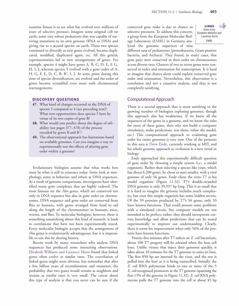
SECTION 11.2 | Synthetic Biology 403
examine fitness is to see what has evolved over millions ofyears of selective pressure. Imagine some original cell onearth, some tiny robust prokaryote that was capable of sur-viving mutations to its own genome (RNA or DNA) andgiving rise to a second species on earth. These two speciescontinued to diversify as new genes evolved, became dupli-cated, modified, duplicated again, etc. All this geneticexperimentation led to new arrangements of genes. Forexample, species 4 might have genes A, B, C, D, E, F, G,H, I, J, whereas species 5 evolved with a gene order of A,H, G, F, E, D, C, B, B�, I, J. At some point during thistime of species diversification, sex evolved and the order ofgenes became scrambled even more with chromosomalrearrangements.
DISCOVE RY QU ESTIONS47. What kind of changes occurred to the DNA of
species 5 compared to 4 (see preceding text)?What new opportunities does species 5 have byvirtue of its two copies of gene B?
48. What would you predict about the degree of reli-ability (see pages 377–378) of the processencoded by genes B and B�?
49. The observational approach has limitations basedon available genomes. Can you imagine a way toexperimentally test the effects of altering geneorder within a genome?
Evolutionary biologists assume that what works bestmust be what is still in existence today. Some look at mor-phology, some at behavior, and others at DNA sequences.As a result of genome comparisons, investigators have iden-tified many gene complexes that are highly ordered. Themost famous are the Hox genes, which are conserved notonly in DNA sequence but also in gene order on chromo-somes. DNA sequence and gene order are conserved fromflies to humans, with genes arranged from head to tailalong the length of the chromosomes in humans, mice,worms, and flies. To molecular biologists, however, there issomething unsatisfying about this kind of research: it leadsto correlations that have not been experimentally tested.Every molecular biologist accepts that the arrangement ofHox genes is evolutionarily advantageous, but it is impossi-ble to test this by altering history.
Recent work by many researchers who analyze DNAsequences has produced some interesting observations.Elizabeth Williams and Laurence Hurst found that linkedgenes often evolve at similar rates. The coevolution oflinked genes might seem obvious, but remember that aftera few billion years of recombination and mutation, theprobability that two genes would remain as neighbors andmutate at similar rates is very small. The caveat aboutthis type of analysis is that you never can be sure if the
conserved gene order is due to chance orselective pressures. To address this concern,a group from the European Molecular Biol-ogy Laboratory (EMBL) in Germany ana-lyzed the genomic sequences of ninedifferent taxa of prokaryotes (proteobacteria, Gram-positivebacteria, and Archaea). They found, in many cases, thatgene pairs were conserved in their order on chromosomesacross diverse taxa. Clusters of two to seven genes were con-served in order and orientation for transcription. It is hardto imagine that chance alone could explain conserved geneorder and orientation. Nevertheless, this observation is acorrelation and not a causative analysis, and thus is notcompletely satisfying.
Computational Approach
There is a second approach that is more satisfying to thegrowing number of biologists exploring genomes, thoughthis approach also has weaknesses. If we know all thesequences of the genes in a genome, and we know the rolesfor most of these genes, then why not build a computersimulation, make predictions, test them, refine the model,etc.? This computational approach to evaluating geneorder for entire genomes is very new. One of the pioneersin this area is Drew Endy, currently working at MIT, andhis whole genome approach to evolution is a new trend inbiology.
Endy approached this experimentally difficult questionof gene order by choosing a simple system (i.e., a modelorganism). Rather than selecting a species like yeast, whichhas about 6,200 genes, he chose to start smaller, with a viralgenome of only 56 genes. Endy chose the virus T7 as hismodel organism (Figure 11.32). T7’s double-strandedDNA genome is only 39,937 bp long. This is so small thatit is hard to imagine the genome includes much complex-ity, but even this simple organism has some hidden secrets.Of the 59 proteins produced by T7’s 56 genes, only 33have known functions. That could present some problemswith a simulated circuit, but computer models are notintended to be perfect; rather, they should incorporate cur-rent knowledge and allow predictions that can be testedexperimentally to improve our understanding. Clearly,there is room for improvement when only 56% of the pro-teins have known functions.
Twenty-five minutes after T7 infects an E. coli bacterium,about 100 T7 progeny will be released when the host celllyses. Unlike viruses that inject their genomes quickly, ittakes about 10 minutes for the T7 genome to enter its host.The first 850 bp are inserted by the virus, and the rest ispulled into the host as it is being transcribed. Initially, the E. coli RNA polymerase binds to one or more of the 5 E. coli-recognized promoters in the T7 genome (spanning thefirst 15% of the genome in Figure 11.32). E. coli RNA poly-merase pulls the T7 genome into the cell at about 45 bp
L I N KSDrew Endy
Elizabeth Williams andLaurence Hurst
EMBL
CAMPMC11_0805382194.QXD 6/12/06 11:56 AM Page 403
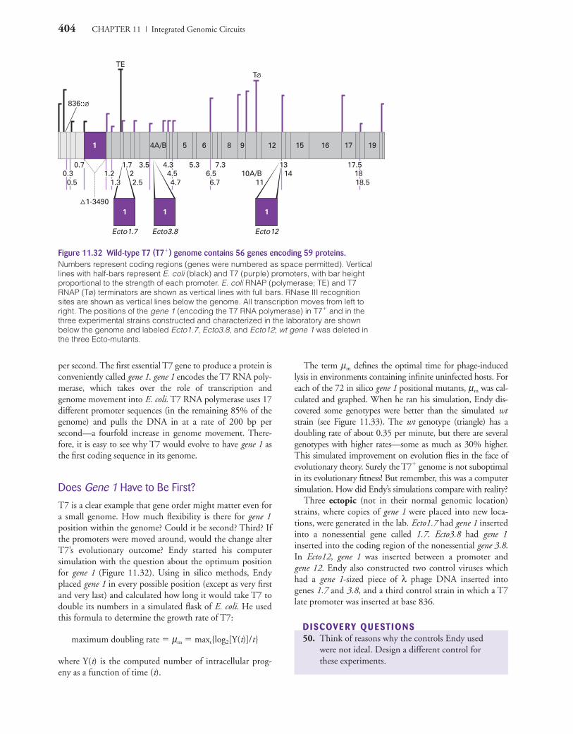
404 CHAPTER 11 | Integrated Genomic Circuits
0.7
1 5 6 8 9 12 15 16 17 194A/B
1.20.32.5 4.7 6.7 11 18.5
2 4.5 6.5 10A/B 14 183.5 4.3 5.3 7.3 17.5
0.5
Ecto1.7 Ecto12Ecto3.8
1 1 1
TET
1-3490
1.3
1.7 13
836::
Figure 11.32 Wild-type T7 (T7�) genome contains 56 genes encoding 59 proteins.Numbers represent coding regions (genes were numbered as space permitted). Verticallines with half-bars represent E. coli (black) and T7 (purple) promoters, with bar heightproportional to the strength of each promoter. E. coli RNAP (polymerase; TE) and T7RNAP (Tø) terminators are shown as vertical lines with full bars. RNase III recognitionsites are shown as vertical lines below the genome. All transcription moves from left toright. The positions of the gene 1 (encoding the T7 RNA polymerase) in T7� and in thethree experimental strains constructed and characterized in the laboratory are shownbelow the genome and labeled Ecto1.7, Ecto3.8, and Ecto12; wt gene 1 was deleted inthe three Ecto-mutants.
per second. The first essential T7 gene to produce a protein isconveniently called gene 1. gene 1 encodes the T7 RNA poly-merase, which takes over the role of transcription andgenome movement into E. coli. T7 RNA polymerase uses 17different promoter sequences (in the remaining 85% of thegenome) and pulls the DNA in at a rate of 200 bp persecond—a fourfold increase in genome movement. There-fore, it is easy to see why T7 would evolve to have gene 1 asthe first coding sequence in its genome.
Does Gene 1 Have to Be First?
T7 is a clear example that gene order might matter even fora small genome. How much flexibility is there for gene 1position within the genome? Could it be second? Third? Ifthe promoters were moved around, would the change alterT7’s evolutionary outcome? Endy started his computersimulation with the question about the optimum positionfor gene 1 (Figure 11.32). Using in silico methods, Endyplaced gene 1 in every possible position (except as very firstand very last) and calculated how long it would take T7 todouble its numbers in a simulated flask of E. coli. He usedthis formula to determine the growth rate of T7:
maximum doubling rate � µm � maxt{log2[Y(t)]/t }
where Y(t) is the computed number of intracellular prog-eny as a function of time (t).
The term µm defines the optimal time for phage-inducedlysis in environments containing infinite uninfected hosts. Foreach of the 72 in silico gene 1 positional mutants, µm was cal-culated and graphed. When he ran his simulation, Endy dis-covered some genotypes were better than the simulated wtstrain (see Figure 11.33). The wt genotype (triangle) has adoubling rate of about 0.35 per minute, but there are severalgenotypes with higher rates—some as much as 30% higher.This simulated improvement on evolution flies in the face ofevolutionary theory. Surely the T7� genome is not suboptimalin its evolutionary fitness! But remember, this was a computersimulation. How did Endy’s simulations compare with reality?
Three ectopic (not in their normal genomic location)strains, where copies of gene 1 were placed into new loca-tions, were generated in the lab. Ecto1.7 had gene 1 insertedinto a nonessential gene called 1.7. Ecto3.8 had gene 1inserted into the coding region of the nonessential gene 3.8.In Ecto12, gene 1 was inserted between a promoter and gene 12. Endy also constructed two control viruses whichhad a gene 1-sized piece of λ phage DNA inserted intogenes 1.7 and 3.8, and a third control strain in which a T7late promoter was inserted at base 836.
DISCOVE RY QU ESTIONS50. Think of reasons why the controls Endy used
were not ideal. Design a different control forthese experiments.
CAMPMC11_0805382194.QXD 6/12/06 11:56 AM Page 404

SECTION 11.2 | Synthetic Biology 405
06020 400 80
0.4
0.2
0.6
0.8
1
Re
lati
ve
pro
ge
ny
pe
r
infe
cte
d h
ost
03010 200 40
0.4
0.2
0.6
0.8
1
03010 200 40
0.4
0.2
0.6
0.8
1
03010 200 40
0.4
Re
lati
ve
pro
ge
ny
pe
r
infe
cte
d h
ost
0.2
0.6
0.8
1
Minutes postinfectionMinutes postinfection
d)
b)
c)
a)
T7+ Ecto1.7
Ecto3.8 Ecto12
Figure 11.34 Computed (solid lines) and observed (black dots) intracellular one-stepgrowth curves for T7�(wt) and the ectopic gene 1 strains.Note the different time scale for Ecto12. a) wt, b) Ecto1.7, c) Ecto3.8, and d) Ecto12 areshown (black), with T7� growth curve (purple line) for reference.
1.7
3.8
12
010 252015 3050 35 40
0.05
0.1
0.15
0.2
0.25
0.3
0.35
0.4
0.45
0.5
Gene 1 position
Maxim
um
do
ub
lin
g r
ate
per
min
ute
Figure 11.33 Predicted consequences of altered gene 1 position.Computed maximum phage doubling rate, µm, as gene 1was repositioned on the T7� genome. Black circles markthe 5� end of the in silico ectopic (inserted) gene 1 and theµm for 72 positional mutants. The purple diamonds indicatethe computed µm for the ectopic gene 1 strains that wereconstructed and characterized experimentally. The purpletriangle indicates the µm computed for T7�.
51. It is difficult to understand what would make amutant strain more efficient, but easier to under-stand less efficient mutants. Explain why themutations with gene 1 positioned late in thegenome would be the least efficient.
52. In the T7 computer simulation,identical viruses were programmedto behave identically. In reality, would you expecteach virus to perform exactly the same? Do youthink stochastic events might occur in naturalsettings? If so, what effect might randomnesshave on the difference between computer growthcurves and real growth curves?
Endy compared the simulated viruses to his three geneti-cally engineered mutant strains of T7. Each real strain wasadded to a separate population of E. coli in a flask, and thereal doubling rates for these T7 mutants were experimen-tally measured (Figure 11.34). The simulated growth curvefor T7� was four minutes faster than the experimentallydetermined growth curve for T7�. Compare the slopes ofcomputer growth rates and the real growth rates for T7,and you will see they are very similar. The simulatedgrowth curve for Ecto12 was ten minutes faster than theexperimentally determined curve. Live Ecto1.7 and Ecto3.8strains showed little agreement with predicted growth rates.
As part of his research, Endy simulated and measuredplaque sizes, DNA replication, protein production, andlysis rates for his three real mutants. Go to the web site toview the T7 simulation (with a link to the 80-MB movie)that shows the rate of transcription and translation forevery gene in the T7 genome. It also shows the E. coli and
DATAT7 simulation
CAMPMC11_0805382194.QXD 6/12/06 11:56 AM Page 405
406 CHAPTER 11 | Integrated Genomic Circuits
T7 RNA polymerases in action. All thiswork indicated that Endy was successful inthe scientific sense. He constructed a model,
made predictions, tested them, and now he will refine hismodel based on new experimental evidence.
DISCOVE RY QU ESTIONS53. Which part of the real curve differs the most
from the simulated curve (see Figure 11.34)?Explain why this part of each curve might be sodifferent, given what you know about stochasticprotein kinetics and noisy toggle switches.
54. Reevaluate the data in Figure 11.33 after analyz-ing the experimental data from Figure 11.34.What can you say about the optimum gene orderfor T7?
55. In the T7 simulation, which is produced ingreater quantities, mRNA or proteins? By the endof infection, which genes are most highly tran-scribed? Which proteins are most abundant?How many copies are present inside the infectedcell for the most abundant protein? At the end ofthe infection, the earliest T7 genes are no longertranscribed. Explain why this may be biologicallyadaptive and why this may indicate why theorder of T7 genes is functionally significant.
56. Can the T7 RNA polymerase transcribe all thegenes, or only the last 85%? In this simulation,what happens when a T7 RNA polymerasecatches an E. coli RNA polymerase from behind?Do you think this is biologically accurate?Explain your answer.
57. Initially, what two proteins are the only onespresent? What happens to each of them duringthe infection?
Endy’s research illustrates how difficult it will be tounderstand more complex genomes. Part of the problemwith T7� is that some genes overlap each other, whichmakes it impossible to mutate one gene but not the other.To address this challenge, Leon Chan and Sriram Kosurigenerated a synthetic T7 (called T7.1) in which every geneis completely separated from its neighbors. T7.1 soundslike a good idea that is bound to fail because synthetic biol-ogists cannot fully understand the selection pressures thathave driven maximization of fitness. However, T7.1 wasviable and produced viable progeny. The plaque size andmorphology were similar to T7�, but the time to lysis wasdelayed for T7.1. As with computer models designed toapproach biological reality, T7.1 is not perfect, but it doesimprove our previous understanding of the naturallyevolved T7�. With T7.1, we will be able to dissect eachcomponent of the genome to understand its function andlater build an improved model of T7 that will test our
newest insights. Over several iterations, T7.n will lead tobetter predictions and a better understanding of genetictoggle switches and synthetic circuits.
DISCOVE RY QU ESTIONS58. You may not realize it, but you can conduct syn-
thetic biology research too. Go to the MITBioBricks Registry to see a community-basedeffort to understand biological circuits andswitches. The concept behind BioBricks is thatDNA parts could be interchangeable, similar toLegos. If you could snap one part onto any otherpart, you could design and construct new devicesand systems to test your understanding of howgenomes perform some of their functions. Trythese tasks to learn your way around. a. Click on “Parts, Devices & Systems” to learn
the vocabulary, and “About Parts” in the left frame to learn what is in the BioBrickRegistry.
b. From the main page, click on the “reporter”icon to see a full list of reporter components.Find GFP and GFP-AAV. What is the differ-ence between these two components?
c. From the main page, enter “BBa_M0044” in the View Part search box on the bottomleft side. What is AAV, and what informa-tion would you like to know that is missing?
d. Click on the “Search” link on the left side,then click on the word “Example” above themiddle search box. The system you havesearched for is composed of four devices.Below it are the intermediate constructionphases that are available in the BioBricksfreezer. Mouse over the icons and see if youcan understand the four devices, as well as theintended function of the overall system. Totest your prediction, enter the term“BBa_I13907” into the search box and readthe description.
59. Information in the Registry may be read by any-one. You can sign up as a guest member andassemble parts in the “sandbox” area of the Registry. Your part numbers have to be in therange designated for nonregistered visitors. Youcan create parts, but they will not be maintainedon the database as a part of the full collection.However, if you find this process interesting, youmight want to join the iGEM competition nextyear to conduct real research in synthetic biology.Although the field is cutting edge, the equipmentrequirements are modest.
DATABioBricks Registry
T7 genes
CAMPMC11_0805382194.QXD 6/12/06 11:56 AM Page 406

References 407
Summary 11.2By applying engineering principles to toggle-switch design,we can construct biologically functional genetic switchesand experimentally test their reliability. It might seemuncomfortable to treat genomes like machines with inter-changeable parts, but by designing and building syntheticdevices and systems, we can test our understanding morecompletely. Whether we assemble three-gene circuits, pro-duce antiswitches to regulate the expression of proteins, orreengineer a model genome as a way of teasing apart thefunction of component parts, we are always trying tounderstand biology and evolution more completely. Even-tually, synthetic biology may lead to new medical treat-ments, but for now, research using designed DNA parts isproving to be challenging and insightful.
Chapter 11 ConclusionsUnderstanding a genome requires more than just listing thecomponent genes and defining their roles. We need tounderstand how the proteins interact, how genes regulateeach other’s transcription, and how positive and negativefeedback loops produce synergistic properties that affect acell’s response to its changing needs. Toggle switches enablegenomes to make “choices,” and the inherent noise in toggleswitches is a necessary part of how they function. Proteinsexhibit stochastic behavior, so it may be impossible to pro-duce a model that can predict with certainty how a particularcell will respond to a change in its environment. Complexcircuits have unique properties, and as we construct increas-ingly complex circuit diagrams, we will discover more emer-gent properties that improve our understanding of cells andorganisms. A cell web is composed of many interconnectedcomponents, and the ultimate challenge is to model thecombined information of genome sequences, variations inthe population, gene expression profiles, proteomics,metabolomics, and genomic circuits. These challenges areintimidating but exciting, too. In Chapter 12, we will useone case study to see what is possible now and where wewant to go in the future.
ReferencesBayer, T. S., & C. D. Smolke. 2005. Programmable ligand-controlled riboregulators of eukaryotic gene expression. NatureBiotechnology. 23(3): 337–343.
Bhalla, U. S., & R. Iyengar. 1999. Emergent properties of networksof biological signaling pathways. Science. 283: 381–387.
Bhalla, U. S., P. T. Ram, & R. Iyengar. 2002. MAP kinase phos-phatase as a locus of flexibility in a mitogen-activated proteinkinase signaling network. Science. 297: 1018–1023.
Bonifer, C. 2000. Developmental regulation of eukaryotic geneloci. Trends in Genetics. 16: 310–315.
Chan, L. Y., Sriram, K., & D. Endy. 2005. Refactoring bacteriophageT7. Molecular Systems Biology 64–73 doi: 10.1038/msb4100025.
Cho, R. J., & M. J. Campbell. 2000. Transcription, genomes,function. Trends in Genetics. 16: 409–415.
Clayton, D. F. 2000. The genomic action potential. Neurobiologyof Learning and Memory. 74: 185–216.
Dandekar, T., M. B. Snel, & P. Bork. 1991. Conservation of geneorder: A fingerprint of proteins that physically interact. Trends inBiochemical Sciences. 23: 324–328.
Edwards, J. S., & B. O. Palsson. 2000. The Escherichia coliMG1655 in silico metabolic genotype: Its definition, characteris-tics, and capabilities. PNAS. 97: 5528–5533.
Edwards, J. S., & B. O. Palsson. 2000. Metabolic flux balance ana-lysis and the in silico analysis of Escherichia coli K-12 gene deletions.BioMed Central Bioinformatics. 1(1): 1. <http://biomedcentral.com/1471-2105/1/1>
Elowitz, M. B., & S. Leibler. 2000. A synthetic oscillatory networkof transcriptional regulators. Nature. 403: 335–338.
Endy, D., & R. Brent. 2001. Modelling cellular behavior. Nature.409: 391–395.
Endy, D., L. You, et al. 2000. Computation, prediction, and exper-imental tests of fitness for bacteriophage T7 mutants with permutedgenomes. PNAS. 97: 5375–5380.
Frankland, P. W., C. O’Brien, et al. 2001. α-CaMKII-dependentplasticity in the cortex is required for permanent memory. Nature.411: 309–313.
Gardner, T. S., C. R. Cantor, & J. J. Collins. 2000. Constructionof a genetic toggle switch in Escherichia coli. Nature. 403: 339–342.
Genoux, D., U. Haditsch, et al. 2002. Protein phosphatase 1 is amolecular constraint on learning and memory. Nature. 418:970–975.
Gladwell, M. 2000. The tipping point: How little things can make abig difference. Boston: Little, Brown.
Hartwell, L. H., J. J. Hopfield, et al. 1999. From molecular tomodular cell biology. Nature. 402 Supplement: C47–C52.
Hasty, J., J. Pradines, et al. 2000. Noise-based switches and ampli-fiers for gene expression. PNAS. 97: 2075–2080.
Hurst, L. D., Williams, E. J. B., & Pál, C. 2002 Natural selectionpromotes the conservation of linkage of co-expressed genes. Trendsin Genetics. 18: 604–606.
Jeong, H. B., R. Tombor, et al. 2000. The large-scale organizationof metabolic networks. Nature. 407: 651–654.
Kelley, B. P., R. Sharan, et al. 2003. Conserved pathways withinbacteria and yeast as revealed by global protein network alignment.PNAS. 100(20): 11394–11399.
Kitami, T., & J. H. Nadeau. 2002. Biochemical networking con-tributes more to genetic buffering in human and mouse metabolicpathways than does gene duplication. Nature Genetics. 32: 191–194.
Kohn, K. 1999. Molecular interaction map of the mammalian cellcycle control and DNA repair systems. Molecular Biology of the Cell.10: 2703–2734.
Kuang, Y., I. Biran, & D. R. Walt. 2004. Simultaneously Monitor-ing Gene Expression Kinetics and Genetic Noise in Single Cells byOptical Well Arrays. Analytical Chemistry. 76: 6282–6286.
Lee, J. F., J. R. Hesselberth, et al. 2004. Aptamer database. NucleicAcids Research. 32(1): D95–100.
Legrain, P., J.-L. Jestin, & V. Schächter. 2000. From the analysis ofprotein complexes to proteome-wide linkage maps. Current Opin-ion in Biotechnology. 11: 402–407.
Lercher, M. J., J-V. Chamary, & L. D. Hurst. 2004. Genomic regionality in rates of evolution is not explained by clustering of
CAMPMC11_0805382194.QXD 6/12/06 11:56 AM Page 407

408 CHAPTER 11 | Integrated Genomic Circuits
genes of comparable expression profile. Genome Research. 14:1002–1013.
McAdams, H., & A. Arkin. 1999. It’s a noisy business! Genetic reg-ulation at the nanomolar scale. Trends in Genetics. 15: 65–69.
McAdams, H., & A. Arkin. 1997. Stochastic mechanisms in geneexpression. PNAS. 94: 814–819.
McAdams, H. H., & L. Shapiro. 1995. Circuit simulation ofgenetic networks. Science. 269: 650–656.
Miller, P., A. M. Zhabotinsky, et al. 2005. The stability of a sto-chastic CaMKII switch: Dependence on the number of enzymemolecules and protein turnover. PLoS Biology. 3(4): 0705–0717.
Milo, R., S. Shen-Orr, et al. 2002. Network motifs: Simple build-ing blocks of complex networks. Science. 298: 824–827.
Murthy, V. L. 2005. The RNA structure database. <www.RNABase.org>. Accessed 20 May 2005.
Pirson, I., N. Fortemaison, et al. 2000. The visual display of regula-tory information and networks. Trends in Cell Biology. 10:404–408.
Ptashne, M. 1987. A genetic switch: Gene control and phage λ. Cambridge, MA: Cell Press & Blackwell Scientific Publications.
Rzhetsky, A., T. Koike, et al. 2000. A knowledge model for analysisand simulation of regulatory networks. Bioinformatics. 16(12):1120–1128.
Suyama, M., & P. Bork. 2001. Evolution of prokaryotic geneorder: genome rearrangements in closely related species. Trends inGenetics. 17(1): 10–13.
Weng, G., U. S. Bhalla, & R. Iyengar. 1999. Complexity in biolog-ical signaling systems. Science. 284: 92–96.
Wray, G. A. 1991. Promoter logic. Science. 279: 1871–1872.
CAMPMC11_0805382194.QXD 6/12/06 11:56 AM Page 408