integrated framework for process and product synthesis/design
TRANSCRIPT

Integrated Framework for Process and Product Synthesis/Design
by
Susilpa Bommareddy
A dissertation submitted to the Graduate Faculty of
Auburn University
in partial fulfillment of the
requirements for the Degree of
Doctor of Philosophy
Auburn, Alabama
December 13, 2013
Keywords: Computer Aided Product Design, Computer Aided Process Synthesis & Design,
Integrated Framework, Group Contribution
Copyright 2013 by Susilpa Bommareddy
Approved by
Mario R. Eden, Chair, Department Chair and McMillan Professor of Chemical Engineering
Christopher B. Roberts, Dean of Engineering and Uthlaut Professor of Chemical Engineering
Allan E. David, John W. Brown Assistant Professor of Chemical Engineering
Nishanth G. Chemmangattuvalappil, Associate Professor of Chemical & Environmental
Engineering, The University of Nottingham

ii
Abstract
Future growth within the chemical process industries depends on various factors such as
raw material and energy availability, sustainability etc. A systematic process synthesis and design
framework integrated with molecular design is needed to synthesize processes that perform this
efficiently. Hence, this dissertation describes the development of a novel hybrid method for
Computer Aided Flowsheet Design (CAFD) and its effective integration with molecular design.
The interactions among process synthesis, process design and molecular design is through a
common set of properties that are employed to analyze the processes as well as external agents
involved in the process. Knowledge of these specific properties is needed to establish the feasibility
of a unit operation in a process and the corresponding conditions of operation. The same
information is needed for design of a component as an appropriate external agent. This forms the
very basis of the proposed hybrid methodology for flowsheet synthesis/design integrated with
molecular design. Both the Computer Aided Flowsheet Design (CAFD) and Computer Aided
Molecular Design (CAMD) frameworks developed are group contribution (GC) based approaches.
CAFD makes use of functional process groups, characterized by the type of unit operation/process
and their corresponding driving force, to generate and represent flowsheets; process group
contribution based property models to predict flowsheet properties from a-priori regressed
contributions of process groups; a notation system (called SFILES) for storing the flowsheet
structural information; and a synthesis method to generate and identify the feasible flowsheets.

iii
The identified candidate flowsheets are ranked based on flowsheet properties (like energy
consumption, amount (mass) of external agents used and/or cost/profit) representing flowsheet
performance in a quantitative sense. Once the promising flowsheet structures are identified, the
flowsheet design parameters that describe the process will be estimated. The reverse simulation
method is used to calculate the design variables of the unit operations involved in the process. This
also gives a good estimate of the important design parameters. Some alternatives may involve unit
operations that require an external agent. Conventional agents may not always meet the property
constraints set by the reverse simulation design problem of such operations. Novel agents can be
identified by solving a product design problem satisfying the property constraints. This is done by
integrating the flowsheet design problem with a molecular design problem. Depending on the type
of unit operation in the process where an external agent is required, the CAMD problem is
formulated accordingly and the effect of the solution alternatives from the CAMD problem on the
process is evaluated by the process models. CAMD includes building blocks (atoms and functional
groups) to generate and represent molecules; group contribution based property models to predict
target properties; a standard molecular structure notation system to store and visualize the
molecular structure information; and a synthesis method to generate and screen molecules that
match the target (design) properties. Once a set of near optimal flowsheet alternatives have been
identified, rigorous simulation is used to verify the predicted performance and select the best
flowsheet. The framework also aims at maintaining a good accuracy of solutions and large
application range. A completely automated tool to perform the above tasks is also developed.

iv
Acknowledgments
I would like to express my profound thanks to my research advisor, Dr. Mario R. Eden, for
his guidance and advice throughout the research work. His encouragement both on academic and
personal front has tremendously contributed towards the completion of my dissertation. My
knowledge and enthusiasm in the area of process and product design has increased significantly
while working under his guidance and am truly fortunate to have had worked with him.
I would like to thank my research committee, Dr. Christopher B. Roberts, Dr. Allan E. David, Dr.
Nishanth Chemmangattuvalappil and Dr. Steven Taylor for their suggestions and critical reading
of my dissertation. Their comments helped me improve and complete this dissertation. I would
also like to express my gratitude to Professor Rafiqul Gani at the Technical University of Denmark
for his suggestions.
My sincere thanks to my friends, co-workers and others at Auburn University. Special thanks to
my parents, Seeta Reddy Bommareddy and Siva Leela Bommareddy, my husband Mallikarjun
Reddy Nagolu and my sister Sudeepthi Bommareddy. This would have been impossible without
all the support and encouragement they have given me. Thanks to the entire Auburn University
Chemical Engineering Department.

v
Table of Contents
Abstract ........................................................................................................................................... ii
Acknowledgments.......................................................................................................................... iv
List of Tables ............................................................................................................................... viii
List of Figures ............................................................................................................................... xi
1. Introduction ............................................................................................................................ 1
2. Theoretical Background ........................................................................................................ 6
2.1 Chemical Process and Product Synthesis/ Design ..................................................... 6
2.1.1 Mathematical Formulation of the Process and Product Synthesis/Design Problem ... 8
2.2 Integrated Process and Product Design ...................................................................... 9
2.2.1 Property Models ........................................................................................................ 11
2.2.2 Reverse Problem Formulation ................................................................................... 13
2.3 Process Synthesis and Design ..................................................................................... 14
2.3.1 Process Integration .................................................................................................... 19
2.4 Computer Aided Molecular Design ........................................................................... 21
2.4.1 Formulation of property constraints .......................................................................... 22
2.4.2 Molecular Design Algorithms ................................................................................... 23
2.4.3 Group Contribution Methods and Property models .................................................. 25
2.5 Summary ...................................................................................................................... 29
3. Computer Aided Molecular Design ..................................................................................... 31
3.1 Molecular Design by decomposition based approach.............................................. 31

vi
3.2 Processing of Molecular Descriptors ......................................................................... 33
3.3 Mathematical model of the molecular design problem ........................................... 40
3.3.1 Problem prerequisites ................................................................................................ 41
3.3.2 Subproblem 1: Maximizing the number of each first-order group that could possibly
appear in the molecule ............................................................................................... 42
3.3.3 Subproblem 2: Enumerating all group subsets of available first-order groups that
could form at least one molecule ............................................................................... 44
3.3.4 Subproblem 3: Estimating possible higher order groups .......................................... 45
3.3.5 Subproblem 4: Eliminating property infeasible group subsets ................................. 48
3.3.6 Subproblem 5: Forming final molecules. .................................................................. 49
3.4 Summary ...................................................................................................................... 50
3.5 Case Studies – Computer Aided Molecular Design ................................................. 50
3.5.1 Case Study – Design of blanket wash solvent ........................................................... 50
3.5.2 Case Study – Design of cyclic molecules ................................................................. 64
4. Property Based Process Design and its Integration with Molecular Design ..................... 71
4.1 Property Operators and Clustering Techniques ...................................................... 71
4.1.1 Intra-Stream Conservation ........................................................................................ 73
4.1.2 Inter-Stream Conservation ........................................................................................ 74
4.2 Process Design by Visualization tools ....................................................................... 75
4.2.1 Identification of feasibility region for sink ................................................................ 75
4.2.2 Source - Sink Mapping .............................................................................................. 77
4.2.3 Identification of feasibility region for fresh source ................................................... 79
4.3 Process Design by Mathematical Programming ...................................................... 80
4.3.1 Mathematical model of the process design problem ................................................. 81
4.3.2 Global optimal solution ............................................................................................. 83
4.4 Framework for Integrated Process and Product Design......................................... 87
4.5 Optimal Solution to Integrated Process & Product Design Problem..................... 89
4.6 Summary ...................................................................................................................... 90

vii
4.7 Case Studies – Integrated Process & Product Design ............................................. 91
4.7.1 Case Study – Design of solvent for a gas treatment process ..................................... 91
5. Integrated Process & Product Synthesis/Design .............................................................. 107
5.1 Framework for Integrated Process and Product Design....................................... 107
5.2 Process Synthesis/Design by decomposition based approach ............................... 111
5.2.1 Methods for selecting/screening unit operations ..................................................... 112
5.2.2 Process Descriptors ................................................................................................. 113
5.3 The CAFD framework integrated with CAMD framework. ................................ 123
5.3.1 Problem Definition & Analysis ............................................................................... 125
5.3.2 Flowsheet Synthesis ................................................................................................ 130
5.3.3 Process Design and integration with Molecular Design ......................................... 138
5.3.4 Final Verification .................................................................................................... 140
5.3.5 Software Implementation ........................................................................................ 140
5.4 Summary .................................................................................................................... 142
5.5 Case Studies – Computer Aided Flowsheet Design ............................................... 143
5.5.1 Case Study – Production of Isobutene .................................................................... 143
5.5.2 Case Study – Production of Diethyl Succinate ....................................................... 150
6. Conclusions ........................................................................................................................ 156
6.1 Achievements ............................................................................................................. 156
6.2 Remaining challenges for CAFD and CAMD framework .................................... 160
7. References .......................................................................................................................... 162
Appendix A. ................................................................................................................................ 173
Appendix B. ................................................................................................................................ 198
Appendix C ................................................................................................................................. 204

viii
List of Tables
Table 2.1: Group Contribution Models ......................................................................................... 27
Table 2.2: Adjustable parameters in Group Contribution Models ................................................ 28
Table 3.1: Values of the Atomic Index 𝜹𝒗 for Each Atom/Vertex (nH is the number of connected
hydrogen atoms) (Gani et al., 2005) ........................................................................... 39
Table 3.2: Classification of Groups (Gani et al., 1991). ............................................................... 40
Table 3.3: Example of enumerated group subset. ......................................................................... 44
Table 3.4: Property targets for Blanket wash................................................................................ 52
Table 3.5: Molecular property targets for blanket wash. .............................................................. 53
Table 3.6: Possible higher order groups for blanket wash case study. ......................................... 56
Table 3.7: Possible blanket wash solvents. ................................................................................... 59
Table 3.8: Vapor pressure and solubility calculations for identified blanket wash solvents. ....... 62
Table 3.9: Property targets for cyclic molecules. ......................................................................... 64
Table 3.10: Molecular property targets for cyclic molecules. ...................................................... 65
Table 3.11: Possible higher order groups for cyclic molecules. ................................................... 67
Table 3.12: Possible cyclic molecules. ......................................................................................... 68
Table 4.1: Property data for gas purification process. .................................................................. 92
Table 4.2: Property targets for fresh solvent. ................................................................................ 94
Table 4.3: Additional property constraints. .................................................................................. 95
Table 4.4: Molecular property targets. .......................................................................................... 97
Table 4.5: Class and Category of selected first-order groups (Gani et al., 1991). ........................ 98
Table 4.6: Possible higher order groups. ...................................................................................... 99

ix
Table 4.7: Valid Molecules for Acid Gas Problem..................................................................... 105
Table 4.8: Source-Sink allocation with molecule 3 as fresh solvent. ......................................... 106
Table 5.1: Available Process groups (Alvarado, 2010). ............................................................. 120
Table 5.2: List of considered pure component properties ........................................................... 127
Table 5.3: Illustration of component order table. ....................................................................... 131
Table 5.4 : Illustration of binary split order table. ...................................................................... 132
Table 5.5: Initialized PGs of a ABC mixture. ............................................................................. 132
Table 5.6: Azeotropes at 1 atm pressure. .................................................................................... 144
Table 5.7: Separation tasks and potential techniques for Isobutene production. ........................ 145
Table 5.8: Design parameters of distillation columns ................................................................ 150
Table 5.9: Separation tasks and potential techniques for DES production ................................. 152
Table 5.10: Initialized process groups for DES production. ....................................................... 152
Table A.1: First order group contribution data (Marrero & Gani, 2001) ................................... 174
Table A.2: Second-order group contribution data (Marrero & Gani, 2001). .............................. 178
Table A.3: Third-order group contribution data (Marrero & Gani, 2001). ................................. 181
Table A.4: Property model for each property(Marrero & Gani, 2001) ...................................... 183
Table A.5: Value of Adjustable Parameters(Marrero & Gani, 2001) ......................................... 183
Table A.6: First-order group contribution data (Marrero & Gani, 2002) ................................... 184
Table A.7: Second-order group contribution data (Marrero & Gani, 2002). .............................. 186
Table A.8: Third-order group contribution data (Marrero & Gani, 2002). ................................. 188
Table A.9: Property Models for properties (Marrero & Gani, 2002). ........................................ 189
Table A.10: First-order group contributions to the dispersion partial solubility parameter, δd , the
polar partial solubility parameter, δp, and the hydrogen-bonding partial solubility
parameter, δhb (Stefanis & Panayiotou, 2008). ......................................................... 190
Table A.11: Second-order group contributions to the dispersion partial solubility parameter, δd ,
the polar .................................................................................................................... 192
Table A.12: Property Models for estimation of Hansen solubility parameters. ......................... 193
Table A.13: Regressed Parameters for the CI Method (Gani et al., 2005). ............................... 193

x
Table A.14: Classification of Groups (Gani et al., 1991). .......................................................... 194
Table A.15: Rules for generation of acyclic molecules(Gani et al., 1991). ................................ 195
Table A.16: Rules for generation of aromatic molecules(Gani et al., 1991). ............................. 196
Table A.17: Rules for generation of cyclic molecules(Gani et al., 1991). ................................. 197
Table B.1: Recommended limits on properties for separation techniques (Jaksland et al., 1995).
................................................................................................................................... 198
Table B.2: Available PGs (Alvarado, 2010; d'Anterroches, 2006). ........................................... 199
Table B.3: Rules to denote PGs by invariants through example(d'Anterroches, 2006). ............ 200
Table B.4: Contributions of the simple distillation process groups (d'Anterroches, 2006). ....... 201
Table B.5: Contributions of the extractive process groups (Alvarado, 2010). ........................... 202
Table B.6: Pre-calculated values based on driving force approach to design simple distillation
columns (Bek-Pedersen, 2003) ................................................................................. 203

xi
List of Figures
Figure 2.1: The product design process (R. Gani, 2004). ............................................................... 7
Figure 2.2: Simultaneous solution of process and molecular design problems (adapted from Eden
(2003)) ....................................................................................................................... 11
Figure 2.3: Reverse problem formulation (adapted from Eden (2003)) ....................................... 14
Figure 3.1: Reverse Problem Formulation of Molecular Design. ................................................. 32
Figure 3.2: CAMD framework ..................................................................................................... 42
Figure 3.3: Method to estimate maximum number of higher-order groups. ................................ 48
Figure 4.1: Ternary representation of clusters and their intra- and inter-stream conservation
characteristics. ........................................................................................................... 73
Figure 4.2: Boundary Feasible region ........................................................................................... 77
Figure 4.3: Source - Sink Mapping ............................................................................................... 78
Figure 4.4: Identification of feasibility region for fresh source (Eljack, Solvason,
Chemmangattuvalappil, & Eden, 2008) .................................................................... 80
Figure 4.5: (a) Reverse Problem Formulation by Eden et al. (2003a). (b) Proposed framework
for simultaneous solution to process & product design problems ............................. 88
Figure 5.1: Relation between properties and process synthesis , design, product design ........... 108
Figure 5.2: Methodology for integrated process and design....................................................... 109
Figure 5.3: Driving force as a function of composition (Bek-Pedersen, 2003) .......................... 115
Figure 5.4: Example of attainable region for the trambouze reaction scheme. .......................... 117
Figure 5.5: Representation of flowsheet (a). with process groups (b, c) process groups ........... 119
Figure 5.6: SFILES notation of a simple flowsheet (a) without recycle (b) with recycle. ......... 122
Figure 5.7: CAFD framework. .................................................................................................... 124

xii
Figure 5.8: Problem analysis steps (Jaksland et al., 1995). ........................................................ 125
Figure 5.9: Initialization of PGs for an mixture encountered in runtime.................................... 133
Figure 5.10: Illustration of PGs superstructure. .......................................................................... 134
Figure 5.11: Generation of superstructure of PGs. ..................................................................... 135
Figure 5.12: (a) Tree representation of a combination, (b) SFILES representation of the feasible
flowsheet ................................................................................................................. 137
Figure 5.13: Algorithm for SFILES generation. ......................................................................... 137
Figure 5.14: Data flow in the CAFD framework. ....................................................................... 141
Figure 5.15: View of the developed CAFD tool ......................................................................... 142
Figure 5.16: Generation of SFILES using the CAFD tool. ......................................................... 146
Figure 5.17: SFILES identified by the CAFD tool for Isobutene production problem. ............. 146
Figure 5.18: Selected optimal flowsheet. .................................................................................... 147
Figure 5.19: Flowsheet from literature (Yamase & Suzuki, 2005)............................................. 149

1
1. Introduction
Design of processes and products is among the most creative of engineering activities with many
opportunities to invent imaginative new products and processes. In simpler terms, it can be viewed
as the effective production of products that meet customer needs through an efficient process. The
question that is addressed in this dissertation is:
“Given the product requirements, determine the optimal process flowsheet to manufacture it.”
Once the identity of the chemical to be manufactured is known, process design involves
determining if it can be manufactured and how. This is the process synthesis and design step.
Again, for the designed process, we also need to determine the likely raw materials to be processed
in order to manufacture the desired product. Apart from the known raw materials there may be
cases where some external agents like mass separating agents etc. are needed in the process.
Specific properties governing the process direct the selection of these agents. These agents can be
identified by a database search but this approach limits the selection of novel compounds. Hence,
this scenario leads to invoking a product design problem.
It is clear that, in most cases process and product design problems cannot be easily decoupled and
hence, a framework capable of effectively integrating process and product design is needed. So, to
be precise the question addressed in this dissertation is:

2
“Given the product requirements, develop a framework for solving process and product
synthesis/design problems and their integration to ultimately identify the optimal process
flowsheet to manufacture it”
Also, traditionally, process/product synthesis and design has been performed in an iterative
fashion. Though this evolutionary method that is forward in nature led to a more sophisticated
design, it could not guarantee that no even better solution exists. If an efficient way to identify
targets beforehand exists, then the iterative nature of solving design problems could be relieved
and process/product specifics resulting in these targets could be identified in a reverse fashion. The
targets enable a performance assessment of the identified solutions. Since it is not possible to
specify the optimum solution apriori from a design perspective, specifying the targets in terms of
desired process/product performance is quite beneficial.
While it should be clear from the discussion above that process and product synthesis/design
should be solved simultaneously as a single problem in order to achieve an optimal solution, the
question of how to handle the complexity of such design problems arises. This issue is solved by
insightfully decoupling the process and product design problems and solving them piecewise based
on a reverse solution methodology (Eden, Jørgensen, Gani, & El-Halwagi, 2004) to achieve their
respective new targets. These new targets are surrogates of the overall design performance target.
The performance specification of a design is often in terms of certain measurable
properties/functionalities rather than the chemical species involved. For example, in the design of
a blanket wash solvent, the primary quality parameters for the designer are the solubility parameter,
flammability, vapor pressure etc. of the solvent. Therefore, a methodology capable of

3
systematically tracking these properties is called for and thus the concept of property
clustering (Shelley & El-Halwagi, 2000) is utilized in this work.
This dissertation introduces a novel hybrid method for Computer Aided Flowsheet Design (CAFD)
effectively integrated with Computer Aided Molecular Design (CAMD). The developed algorithm
systematically identifies feasible process flowsheets in a computationally efficient manner by
combining physical insights with algorithmic reverse design approaches. In the reverse approach,
the flowsheets meeting the desired process performance are identified. Then, the design variables,
which facilitate the desired process performance and the molecules that satisfy the property targets
identified by solution of the process design problem are found. Both CAFD and CAMD
methodologies are based on group contribution (GC) approaches. In these approaches, various
groups (molecular fragments/flowsheet fragments) are tabulated along with their contributions
towards a property of the molecule/flowsheet that includes these fragments. These contributions
are estimated through regression of large amounts of experimental data. The property model
equations for a set of tabulated data depend on how these values are regressed and are unique with
respect to each set of GC data. Hence utilizing these tabulated data and respective models,
methodologies to solve process and product design problems in a reverse fashion are developed.
Doing so, the evaluation of solution alternatives of each with reference to their respective targets
is straightforward given the models and the group contributions. A simple notation system,
SFILES is employed for efficient storage and transfer of flowsheet information. The design
variables for the selected flowsheet(s) are identified through a reverse simulation approach. Once
the design parameters of an optimal flowsheet alternative have been identified, rigorous simulation
is used to verify the predicted performance.

4
By solving the integrated process and product synthesis/design problems this way, the effect of
any changes in the products on the process as well as the effect of changes in the process on the
products can be rapidly evaluated. As an additional benefit the process and product design
problems are selectively decoupled, so the solution is achieved with less complexity.
The solution methodology for process and product design problems and their simultaneous
solution presented in Chapters 3 & 4. The work was published in Computer Aided Chemical
Engineering as well as Computers & Chemical Engineering (Bommareddy,
Chemmangattuvalappil, Solvason, & Eden, 2009b, 2010b). Complete description of the CAMD
framework with respect to how the first- and higher- order groups from the group contribution data
are incorporated in the different stages of framework was published in the Brazilian Journal of
Chemical Engineering and the book Design for Energy & the Environment (Bommareddy,
Chemmangattuvalappil, Solvason, & Eden, 2009a, 2010a). Detailed discussion of the CAFD
framework and a completely automated tool to perform the above tasks was developed and
published in Computer Aided Chemical Engineering (Bommareddy, Eden, & Gani, 2011). Also
the integrated framework for process and product synthesis/design was published in Computer
Aided Chemical Engineering (Bommareddy, Chemmangattuvalappil, & Eden, 2012)
The dissertation has been distributed in five chapters: Chapter 2 covers most of the background
information including a discussion of the nature of process and product synthesis/design problems,
current product design techniques, and basics of group contribution methods. Chapter 2 also covers
the role of property models, the concept of reverse problem formulations and the state of art of
process and product synthesis/design problems. Chapter 3 describes the development of a new
CAMD framework and its application examples. Chapter 4 starts with the basics of property
clustering and process design by both visualization and mathematical methods. Then, it covers the

5
systematic procedure for integrating process and product design and gives a case study to explain
its application. Chapter 5 provides the process synthesis and design (CAFD) framework and its
integration with CAMD followed by the software implementation of the developed methodology.
Finally, two application examples for the algorithms developed in the chapter are given. The last
chapter describes the major achievements and conclusions from this work followed by the next
steps to be undertaken as part of this work. Finally the dissertation is appended with the data used
from literature.

6
2. Theoretical Background
2.1 Chemical Process and Product Synthesis/ Design
Chemical product design, as quoted by Moggridge and Cussler (2000) is comprised of four steps:
“The first step is the identification of customer needs and the translation of the needs into product
specifications. The second step involves generating and winnowing ideas to fill these needs. In the
third step the best ideas are chosen for commercial development. The last step requires product
prototyping, decisions on manufacturing route and estimation of economic boundaries”. Although
this design scheme is simplified and thus applicable to many product design problems, it needs to
be more clearly defined to adapt it to different cases of problems.
The second and third steps comprise the product design problem, the first step is a pre-design step
or problem formulation step and the last step is part of a process design problem. Traditionally
process and product design problems have been treated as two separate problems, with little or no
feedback between them. Product design has been carried out based on heuristics and expert
knowledge to provide options that match the requirements. The compounds identified in this step
are analyzed to decide on their suitability and if an efficient manufacturing route to make it exists.
If none of the options are practical, the product design problem is redone with looser constraints.
Therefore, this is an iterative process as described in Figure 2.1.

7
Figure 2.1: The product design process (Gani, 2004).
The other way of analyzing the need for integration of process and product synthesis/design
problems is listed below. If we arrive at a stage, where we know the product satisfying the target
specifications and what raw materials could be treated physically or chemically to produce the
product, the remaining task is to design the process to manufacture it. This task involves
synthesizing the process alternatives and designing the selected process. One of the important
factors that decide the selection of one of the synthesized processes is the choice of chemicals used
as external agents (if appropriate) in the process. The steps of synthesizing and designing the
process and design of chemicals to be used are fairly interlinked. As cited in the introduction of
this dissertation, if the two steps are solved to together, the problem becomes fairly complex. If
they are decoupled and solved without analyzing, each of the problems as shown in Figure 2.1
falls prey to the iterative nature of the problem. Hence these problems have to be carefully
decoupled such that targets for each of the decoupled problems are functions of the ultimate
performance targets and the methodologies developed for each of them serve to provide solutions
that match their respective targets.
It is clear that when process and product design problems are solved together, each benefit from
the other to yield truly optimal solutions that meet the performance target(s) but the identification
of such optimal solutions is challenging. Hence methods to address this issue are presented in this
dissertation.

8
2.1.1 Mathematical Formulation of the Process and Product Synthesis/Design Problem
This dissertation addresses some of the issues in process and product synthesis/design by setting
up a mathematical model describing the problem and identifying the solutions. All different types
of product-process design problems can be represented using the following set of mathematical
expressions (Gani, 2004).
𝐹𝑜𝑏𝑗 = 𝑚𝑎𝑥[𝐶𝑇𝑦 + 𝑓(𝑥)] 2.1
Subject to: ℎ1(𝑥) = 0 2.2
ℎ2(𝑥) = 0 2.3
ℎ3(𝑥, 𝑦) = 0 2.4
𝑙1 ≤ 𝑔1(𝑥) ≤ 𝑢1 2.5
𝑙2 ≤ 𝑔2(𝑥, 𝑦) ≤ 𝑢2 2.6
𝑙3 ≤ 𝐵𝑦 + 𝐶𝑥 ≤ 𝑢3 2.7
where,
x : Vector of continuous variables like fraction of a mixture, flow rates etc.
y : Vector representing the presence or absence of a group, compound,
operation, etc.
h1 (x) : Set of equality constraints corresponding to process design specifications.
h2(x) : Set of equality constraints corresponding to process model equations.
h3(x, y) : Set of equality constraints related to molecular structure generation,
mixing rules for properties, etc.
g1 (x) : Set of inequality constraints related to process design specifications.

9
g2(x, y) : Set of inequality expressions corresponding to specific problems related to the
product design.
f(x) : Vector of objective functions.
Many variations of the above mathematical formulation may be derived to represent problems and
their corresponding solution methodologies (Gani, 2004). Some examples are:
1. Solve all the equations. This represents an integrated process-product design problem. The
combined problem represents a complex mixed integer non-linear programming problem.
2. Only satisfy the constraints in Equations 2.2 – 2.7. This generates a feasible set of products
and their corresponding process. Aspects of product-process design are considered
simultaneously.
3. Solve a mathematical programming problem that includes Equations 2.1, 2.4 and 2.6. This
is optimal product design of the molecule and/or mixture.
4. Satisfying the constraints in Equations 2.4 and 2.6. This is a chemical product design
problem that generates molecular structures (or mixtures of molecules) and identifies a set
of feasible candidates.
5. Satisfying only constraint 2.6. This represents a product design problem solution based on
a database search.
2.2 Integrated Process and Product Design
The traditional solution methods to identify optimum solutions to integrated product and process
design problems are forward and iterative in nature and thus may be cumbersome. Hence,
identifying process/product performance targets beforehand and matching the solution alternatives

10
with the targets would make the solution methodology more efficient. This methodology can be
stated as a reverse problem formulation. Also, as discussed in section 2.1, when process design
and molecular design are handled separately, each of them have inherent limitations due to the
nature of their input data. Solving process synthesis/design problems separately would require
committing to specific raw materials well in advance in order to reach a solution. On the other
hand, in molecular design problems, the desired target properties (dependent on the process) are
required input to the solution algorithm. These decisions regarding the input data to the respective
problems are made ahead of design and are usually based on experience and thus could possibly
yield a sub-optimal design.
To overcome the limitations encompassed by decoupling the process and molecular design
problems, a simultaneous approach as outlined in Figure 2.2 has been proposed (Eden, 2003).
Using this approach, the molecular building blocks and the desired process performance are given
as input to the integrated design problem. The final outputs of the algorithm are the design
variables, which facilitate the desired process performance target(s) and the molecules that satisfy
the property targets identified by solution of the process design problem.

11
Figure 2.2: Simultaneous solution of process and molecular design problems (adapted from Eden (2003))
As explained in section 2.1.1, when process and product design problems are solved
simultaneously, the models involved tend to be highly non-linear. The concept of reverse problem
formulation (RPF) has helped formulate integrated process-product design problems without
leading to MINLP formulations by insightful decoupling of the constitutive equations (property
models) from the process model (Eden, Jørgensen, Gani, & El-Halwagi, 2003a). Reverse problem
formulation enables design of novel molecules and solution of process design problems without
commitment to specific components during the solution step. One of the challenges in applying
such a method is that, the process design problem is solved in terms of the properties and not in
terms of components. A systematic way to track properties is presented in the chapter 4.
2.2.1 Property Models
Any mathematical model for a product or process consists of three types of equations, i.e. balance
equations, constitutive equations and constraint equations (Russel, Henriksen, Jørgensen, & Gani,

12
2002). The constitutive equations consist of a set of selected property models which play different
roles in the simulation and design calculations (Gani & O'Connell, 2001). The service role by
property models is when model parameters are given and the process/product model requests the
property values. These types of models are used primarily in process simulators. The service and
advice role is played by property models in process design and synthesis problems. Process design
and synthesis problems are solved in two steps – (a) a step where alternatives are generated – the
property models attempt to identify constraints on feasible conditions of operation and optimum
values of process conditions thus providing advice to the synthesis and design algorithms in terms
of eliminating infeasible solutions; and (b) a step where properties are determined and alternatives
are verified – the property models play only a service role here. Since the property model can
provide design targets along with constraints on feasible property values, it is possible to include
the property model as a part of the solution routine, thus adding a solve role to the service and
advice roles.
When property models (constitutive equations) are used in the solve role, they are decoupled from
the process model and solved separately (Eden et al., 2004). Furthermore it must be emphasized
that by performing this decoupling, the information flow to and from the property model is also
reversed, i.e. the process model is solved for the values of the constitutive variables (properties),
and then the property model is solved to yield the corresponding intensive variables, e.g. process
conditions, process flowsheets or products (including molecular structures). Also, by setting up
the problem to use the property model in the solve mode, it is possible to use different property
models for same variable at different stages of the solution.
Knowledge of some common specific properties (constitutive variables) is needed to establish the
feasibility of a unit operation in a process and the corresponding conditions of operation. The same

13
information is needed for design of a component as an appropriate external agent. Hence, the
constitutive variables that are used to analyze the processes and products in a system allow process
synthesis, process design and molecular design problems to interact with each other.
2.2.2 Reverse Problem Formulation
A mathematical model consisting of balance equations, constraint equations and constitutive
equations may be a mixed integer non-linear problem. Though several techniques to handle these
kinds of problems are available, in practice, these problems tend to be really hard to solve: they
combine the combinatorial nature of mixed integer programming and intrinsic difficulty of
nonlinear programs. Decoupling the equations involved in the model and solving them piecewise
in an integrated fashion to achieve a common constitutive variable would be an efficient way of
solving these models (Eden et al., 2004).
The procedure developed by (Eden, 2003) as illustrated in Figure 2.3 for decoupling the
constitutive equations assists in solving the MINLP formulations. The decoupling of the
constitutive equations as illustrated provides the foundation for two reverse problem formulations:
1. Given input stream(s) variables, equipment parameters and known output stream(s)
variables, determine the constitutive variables.
2. Given values of the constitutive variables, determine the unknown intensive variables
(from the set of temperature, pressure and composition) and/or flowsheet structure and/or
product.

14
Figure 2.3: Reverse problem formulation (adapted from Eden (2003))
As the complex constitutive equations are separated from the model, the solution step to the first
reverse problem is easy. In addition, for the second reverse problem, any number of property
models can be used (as needed to describe entire processes) as long as the target constitutive
variable values identified by the first reverse problem are matched. It is possible to have more than
one solution since the algorithm involves a matching procedure. Therefore, a performance index
can be defined and evaluated for all identified solutions to determine the optimal solution.
2.3 Process Synthesis and Design
Process synthesis and design deals with the determination of an optimal flowsheet configuration
including the required tasks, appropriate equipment capable of converting the feed streams to
product streams. In addition, the design of the equipment and their operating conditions need to be
determined. Once a feasible flowsheet has been identified, it is analyzed/tested to make sure the
process objectives are met. Finally, to gain this detailed understanding of how the process behaves

15
and whether the process objectives are met, process analysis tools such as ASPEN Plus, PRO II,
and HYSYS are often utilized (El-Halwagi, 2006).
Approaches for process synthesis and design include:
a. Heuristic and Knowledge-based Approaches: These approaches are based on a set of rules
developed through experience and available data. In such methods, basically the available
knowledge (e.g., known operation tasks or processes for achieving a particular task) is first
captured in a systematic manner and mined appropriately for a specific problem based on
certain rules and procedures and finally this knowledge is applied to the problem. Hence, such
methods, when automated, mimic the human approach to solving these problems, where
humans search for relevant existing data and apply useful information from it to the current
problem. These rules help in fixing some discrete variables in advance, leading to a reduction
in the size of the solution search space. Without these rules, design problems can often be too
difficult to converge and/or too large to search, however here again the optimality of the
generated solution may not guaranteed (Westerberg, 2004). Also the rules sometimes may be
contradictory as the context in which they can be applied is not necessarily fully defined and
this approach is useful only in cases when the problem to be solved is similar to previously
solved problems (El-Halwagi, 1997). One of the methods meeting this criterion is the one
developed by Douglas (1985). This framework is for separation system design and the
framework is divided into two parts, namely vapor and liquid recovery, and each part is
governed by a set of heuristic rules for the selection of separation tasks. Several solution
techniques along the same lines have also been developed (Barnicki & Fair, 1990, 1992; Chen
& Fan, 1993). In a strategic process synthesis method developed by Siirola (1996), a library of

16
various sets of unit operations called “islands” are made; critical unit operations are selected
from these islands and are interconnected to obtain the final process flowsheets.
b. Mathematical optimization approaches: Here the process synthesis and design problem is
solved using optimization techniques. These methods usually need to obtain a superstructure
of all possible alternative flowsheets. Hence, the optimality of the solution solely depends on
the comprehensiveness of the mathematical superstructure. Usually, representation of such
large optimization problems is in the form of Mixed Integer Non-Linear Programs (MINLPs)
which are computationally intensive, requiring efficient solvers to obtain a global optimal
solution. The MINLP problem as described by Grossmann, Aguirre, and Barttfeld (2005)
involves discrete linear variables (y) and continuous non-integer variables (x,) as shown below.
The goal of the MINLP formulations is to maximize/minimize one or more of the process
specifications, e.g. minimizing cost, maximizing throughput, and/or efficiency etc.
𝐹𝑜𝑏𝑗 = 𝑚𝑖𝑛[𝐶𝑇𝑦 + 𝑓(𝑥)] 2.8
Subject to:
ℎ(𝑥) = 0 2.9
𝐵𝑦 + 𝑔(𝑥) ≤ 0 2.10
𝑥 ∈ 𝑋, 𝑦 ∈ {0,1}𝑚 2.11
The mathematical superstructure determination has been addressed by Friedler, Tarjan, Huang,
and Fan (1993) using a graphical approach. Shah and Kokossis (2002) proposed a task based
approach, where tasks represent simple and/or complex distillation column configurations, to
generate the superstructure and the corresponding MINLP formulation. McCarthy, Fraga, and
Ponton (1998) introduced an automated procedure for product separation synthesis. First, the

17
procedure performs an in-depth tree search to locate solutions and unit operations, applying
design variable discretization to reduce the search space. This methodology has the benefit of
avoiding mapping into an apriori generated superstructure. In all these methods, the algorithm
generates a set of good, feasible solutions which may be further optimized by continuous
means.
c. Hybrid methods: The hybrid approaches combine functionalities of the different approaches
described above into one. Often these methods combine the physical insights of knowledge
based methods with mathematical programming techniques to formulate and solve process
synthesis and design problems. While the simplicity of the knowledge-based methods is carried
into these hybrid techniques, rather than heuristics, fixed rules and guidelines based on
physico-chemical properties of the components involved in the process are used for process
synthesis and design.
In this section, thermodynamic insights based process synthesis of separation processes, the
driving force based synthesis and design of separation processes and attainable region analysis
for reactor network design are discussed.
Thermodynamic insights based flowsheet synthesis:
Jaksland, Gani, and Lien (1995) developed a method that uses thermodynamic insights for
synthesis of separation processes rather than relying on heuristics. The knowledge about a
process is retrieved from the physico-chemical properties of the components in the mixture.
This method is hierarchical and consists of two main levels: a) the first level calculates the
difference in component properties as ratios over a wide range of properties, which in turn
are used as a screening criteria to identify the feasible separation techniques. The separation
technique is selected in such a way that it exploits the largest property differences between

18
components of the mixture to be separated. b) in the second level, a detailed mixture
analysis is done for further screening. If any external mass separating agents are required
in the process, the process design problem is integrated with a molecular design problem.
Driving force based process synthesis and design:
Gani and Bek-Pedersen (2000) introduced the concept of driving force based separation
design. The method developed enables fast and easy identification of near optimal design
without having to resort to computationally intensive calculations. The Driving Force (DF)
for any separation task to be carried out by a given separation technique is the difference
in technique specific chemical/physical properties between two coexisting phases that may
or may not be in equilibrium. Hence, when the DF is used as selection and sequencing
criterion, such that the maximum driving force is utilized at all stages of the process, the
most efficient separation system is quickly found. Also, the design of each separation unit
(e.g. the number of plates in a column, feed location, solvent requirement and its properties
etc.) is evaluated as a function of the maximum driving force. By targeting each unit
operation at the largest possible driving force, a near optimal separation sequence can be
obtained.
Attainable region for reactor networks:
Horn (1964) introduced a concept called attainable region (AR) analysis which enables
simpler, easier, and more robust reactor design and optimization. In attainable region
analysis, all possible output concentrations in the stoichiometric subspace from different
reactor configurations are determined apriori and the optimal reactor network is found from
it. Approaching the problem from this direction ensures that all reactor systems are
included in the analysis. There are several examples of methods for the construction of

19
such regions, e.g. the geometric approach by Glasser, Crowe, and Hildebrandt (1987) and
the algorithmic method presented by Hildebrandt and Biegler (1995). Once the attainable
region is identified, graphical analysis and solution of simple problems is relatively easy
and in the case of more complex problems, the AR can assist in the formulation of the
constraints in a mathematical optimization problem.
The integrated approach by Hostrup (2002) combines the thermodynamic insights of Jaksland
et al. (1995) and Gani and Bek-Pedersen (2000) with the formulation of structural optimization
problems, thus allowing for efficient screening among the alternative routes. d’Anterroches
and Gani (2005) provided the basis for a computer aided flowsheet design (CAFD) framework
based on group contribution approaches. In this group contribution approach, process groups
with their apriori regressed property contributions are used as building blocks. CAFD is solved
in a reverse fashion which enables their easy integration with CAMD. In the hybrid methods,
the flowsheet synthesis problem is solved as a reverse property prediction problem. Here, given
the property target values and/or their functions, the unknown process configurations that
match the property targets are identified. The flowsheet design problems are solved by reverse
simulation formulations. Here, the design variables are back calculated from the simulation
models.
2.3.1 Process Integration
Since chemical processes are integrated systems of interconnected units and streams, an effective
process is possible only by accounting for process integration. Process integration is a holistic
approach to process design, retrofitting and operation which emphasizes the unity of the process
(El-Halwagi, 1997). Based on the two main commodities consumed and processed in a typical
facility, namely mass and energy, process integration is categorized into mass integration and

20
energy integration. Mass integration is a systematic methodology that provides the fundamental
understanding of the global flow of mass within the process and employs this understanding in
identifying the performance targets and routing the species in a process. Energy integration, on the
other hand provides an understanding of energy utilization within the process, thus using it to
identify energy targets and optimize heat-recovery and energy-utility systems. There is a rich
volume of information available in literature that covers the development and uses of energy and
mass integration tools (Cerda, Westerberg, Mason, & Linnhoff, 1983; Dunn & Bush, 2001; El-
Halwagi, 1997; Gundersen & Naess, 1988; Linnhoff & Hindmarsh, 1983; Shenoy, 1995). Many
processes are driven and governed by properties or functionalities of the streams and not by their
chemical constituency. Constraints on process units that can accept recycled/reused process
streams and wastes are not limited to compositions of components but are also based on the
properties of the feeds to processing units (El-Halwagi, 2006). Since properties (or functionalities)
form the basis of performance of many processes, design procedures based on key properties
instead of key compounds are used. But, unlike mass, properties are not conserved and cannot be
tracked among units without undertaking component material balances. Therefore, to resolve these
limitations, conserved property-based clusters are used (Shelley & El-Halwagi, 2000).
Section 2.3 gave an overview of currently utilized process synthesis and design methods. The next
sections will concentrate on the methodologies in molecular design algorithms, and the importance
of property models for molecular design.

21
2.4 Computer Aided Molecular Design
Traditionally the search for solvents or products for specific applications has been carried out by
looking for them in a database of known compounds. A more systematic way to finding a solution
to such problems is computer aided molecular design (CAMD). However, both approaches need
thorough experimental validation before they are put to use. By following a systematic approach
one would be able to look for novel compounds and also trim the list to be experimentally tested
by an exponential factor in comparison to the traditional methods. By definition, a CAMD problem
is (Brignole & Cismondi, 2002): Given a set property constraints, determine the molecule or
molecular structure that matches these desired physico-chemical and/or environmental properties.
The structures of the compounds are represented using descriptors along with an algorithm that
identifies these descriptors. This means the property evaluation methods would also be based on
these descriptors.
The general approach to solving a CAMD problem is to first generate feasible molecular structures
using the set of descriptors (also called building blocks) and then testing them by estimating their
desired properties. These properties are estimated based on the apriori calculated values for each
descriptor participating in a molecular structure. The set of feasible compounds are identified as
those that match the property specifications. The optimal among them is obtained through a
problem specific selection criterion. The principal differences between various CAMD
methodologies are how the various steps in CAMD are performed, the type of descriptors used
and how the necessary property values are obtained. In the method developed in this dissertation
(see Chapter 3), CAMD includes building blocks (first- and higher-order groups) used to generate
and represent molecules; group contribution based property models to predict target properties

22
(Marrero & Gani, 2001); and a synthesis method to generate and screen molecules that match the
target (design) properties.
2.4.1 Formulation of property constraints
A set of properties with specific goal values or lower/upper bounds are identified here and are
problem specific, e.g. if a given chemical must be liquid at certain conditions it should be translated
into constraints on melting and boiling temperature. The property values can be directly
determined through a property model. Some properties however, cannot be explicitly described in
this way, e.g. smell, taste, etc. These properties can in some cases be represented as a function of
explicit properties.
While formulating these constraints, the questions below could help to define the design
boundaries (Harper, 2000):
a. Is the compound a replacement for another compound?
If yes, the constraints can be selected similar to or better than those of the existing
compound based on its drawbacks.
b. What would be the operational limits?
These limits help in defining the upper and lower limit of the constraints on the phase and
the phase transition related properties.
c. What criteria should be used to evaluate the performance of the desired product?
The performance criteria are related to the function of the desired product in the process
for which it is being designed. Sometimes, models for evaluation of performance may be
very complex.
d. Are there any downstream processing considerations?

23
When compounds are designed to play a role in downstream processes, in order to obtain
a global solution to the CAMD problem, the operational limits of the compounds need to
be extended to cover additional possible operations and consequently, other properties may
also have to be considered. The possible utilization of available process streams to be
mixed with the new compound can be studied here. Due to the evident link between process
and product, the molecular design and process design problems should be integrated.
Having the property constraints in hand from the above set of questions and estimation methods
to predict the selected properties, an appropriate molecular synthesis algorithm is needed to obtain
a CAMD solution.
2.4.2 Molecular Design Algorithms
All CAMD algorithms reported in literature, fall into three main categories: mathematical
programming, stochastic optimization, and enumeration techniques (Harper, 2000).
a. Mathematical programming: In solving CAMD problems using optimization
(mathematical programming) techniques, the property constraints identified are used as
mathematical bounds and the performance requirements are defined by an objective
function. Solutions techniques to such optimization problems in general involve solving
Mixed Integer Non-linear Programming (MINLP) models. Although widely used and
proven to be effective, MINLP methods suffer from a large computational load and lack
the guarantee of finding a globally optimal solution. (Duvedi & Achenie, 1996;
Pistikopoulos & Stefanis, 1998; Vaidyanathan & El-Halwagi, 1994).
b. Stochastic optimization: Using this method, the solution alternatives are generated by
trying random variations of the current solution. Analogous to general optimization
problems, this method also aims at finding the optimal value for the objective function, but

24
the technique it uses varies. The nature of the solution methodology involved here gives
the freedom to specify discontinuous properties as the involved optimization methods do
not require any gradient information. There are two forms of stochastic optimization based
CAMD algorithms: a) A simulated annealing approach that has the ability to easily deal
with highly non-linear models (e.g. predictive property models) and large numbers of
decision variables (e.g. numerous alternative molecular structures). “The algorithm runs as
an iterative process in which, possible parameter modifications generate new parameter
values, according to a set of perturbation probabilities” (Marcoulaki & Kokossis, 1998).
The generated parameters are tested against previous values in each iteration to satisfy a
probability criterion. b) A genetic algorithm approach in which a population of possible
solutions (called individuals) is evolved toward better solutions. The evolution usually
starts from a set of randomly generated individuals and is an iterative process, with the
population in each iteration being called a generation, where the individuals exist based on
“survival of the fittest”; i.e. the more fit individuals, usually based on objective function
value, are selected from the current population and each individual is modified to form a
new generation. Because of the stochastic nature, both approaches are capable of handling
non-linear models, although as the problem complexity increases, the genetic algorithm
approach reports challenges in terms of computational time (Marcoulaki & Kokossis, 1998;
Venkatasubramanian, Chan, & Caruthers, 1994).
c. Enumeration techniques: Here the structurally feasible molecular structures based on group
contribution methods are first generated using a combinatorial approach and are then tested
against the specifications, where molecules that fail to satisfy the constraints are
eliminated. As with stochastic optimization, no gradient information is needed here but the

25
disadvantage is that solving a CAMD by simple enumeration may lead to combinatorial
explosion (Constantinou, Bagherpour, Gani, Klein, & Wu, 1996; Friedler, Fan, Kalotai, &
Dallos, 1998; Gani, Nielsen, & Fredenslund, 1991; Joback & Stephanopoulos, 1995).
Using some rules, however, this method can be made more effective. This dissertations
aims at framing such rules and solving CAMD by rule based enumeration and test methods.
A new “generate and test” method was introduced by Harper (2000). Here, the feasible
formulations are generated from molecular building blocks using a rule based
combinatorial approach. This method uses a multi-level CAMD approach that controls the
generation and testing of molecules. Chemmangattuvalappil, Eljack, Solvason, and Eden
(2009) also developed an enumeration and test CAMD algorithm which considers
proximity effects of the atoms participating in a molecule.
2.4.3 Group Contribution Methods and Property Models
Many CAMD techniques use group contribution methods (GCM) to synthesize molecules and
verify whether the generated molecules exhibit the specified set of desirable properties. These
techniques prove to be powerful tools for primary estimation of reasonably accurate results for
many property values when experimental data is not readily available. Generally in these kinds of
methods, various groups (molecular fragments) are tabulated along with their contributions
towards a property of the molecule possessing these fragments. These contributions do not depend
on the position of the fragment in the molecule or nature of the molecule in which it exists. These
contributions are estimated through regression of large amounts of experimental data. The
property model equations for a set of tabulated data depends on how these values are regressed
and are unique with respect to each set of GCM data.

26
In the case of simple compounds, GCM can provide accurate trends. However, as the complexity
of the molecule increases, the accuracy of first order GCM becomes less reliable. They generally
cannot capture proximity effects or differentiate between isomers (Kehiaian, 1983; Wu & Sandler,
1989, 1991). So, several attempts have been made to make the GCM more general and reliable
(Constantinou, Prickett, & Mavrovouniotis, 1993; Fedors, 1982). The ABC method introduced by
Constantinou et al. (1993), though computationally challenging, provided the basis for future GC
methods. The ABC method is based on the contributions of atoms and bonds towards the properties
of different conjugate forms of a molecular structure. Here, the property of a molecule has been
estimated as the linear combination of contributions from all the conjugate forms of the molecule.
Group Contribution models with higher levels:
In the GC approach by Constantinou and Gani (1994), where, property estimation is done in two
stages, two types of molecular building blocks have been defined: first- and higher-order groups.
The higher-order groups give an idea about different types of interactions among the first-order
groups and the effects of certain molecular group combinations to the property of the final
molecule and could possibly differentiate among isomers. The higher-order groups enable a good
representation of poly ring compounds and open-chain polyfunctional compounds (Marrero &
Gani, 2001). The molecular groups from Marrero and Gani (2001) are used in the methodology
developed in this dissertation and their definition and classifications/contributions are provided in
Appendix A.
The property estimation model suggested in this approach has the following form:
𝑓(𝑋) =∑𝑁𝑖𝐶𝑖𝑖
+ 𝑤∑𝑀𝑗𝐷𝑗𝑗
+ 𝑧∑𝑂𝑘𝐸𝑘𝑘
2.12
where,

27
f(X) is a function of the actual property X, Ci is the contribution of first order group i that occurs
Ni times, Dj the contribution of second order group j that occurs Mj times and Ek the contribution
of third order group k that occurs Ok times in the molecule. The constants w and z can have values
of zero or unity depending on how many levels of estimation are of interest.
The primary properties and the corresponding property functions when using Marrero and Gani
groups are listed in Table 2.1. The universal constants for each property function are given in Table
2.2. There are several secondary properties like vapor pressure, flash point, etc. that can be
estimated as functions of primary properties. It should be noted that the application of group
contribution based CAMD techniques rely on the availability of molecular groups and the
estimated property contributions corresponding to each group.
Table 2.1: Group Contribution Models
Property Property function Group contribution terms
Normal melting
point, Tm
exp(𝑇𝑚𝑇𝑚0
) ∑𝑁𝑖𝑇𝑚1𝑖𝑖
+∑𝑀𝑗𝑇𝑚2𝑖𝑗
+∑𝑂𝑘𝑇𝑚3𝑖𝑘
Normal boiling point,
Tb
exp(𝑇𝑏𝑇𝑏0) ∑𝑁𝑖𝑇𝑏1𝑖
𝑖
+∑𝑀𝑗𝑇𝑏2𝑖𝑗
+∑𝑂𝑘𝑇𝑏3𝑖𝑘
Critical temperature,
Tc
exp(𝑇𝑐𝑇𝑐0) ∑𝑁𝑖𝑇𝑐1𝑖
𝑖
+∑𝑀𝑗𝑇𝑐2𝑖𝑗
+∑𝑂𝑘𝑇𝑐3𝑖𝑘
Critical pressure, Pc 1
√(𝑃𝑐 − 𝑃𝑐1)− 𝑃𝑐2 ∑𝑁𝑖𝑃𝑐1𝑖
𝑖
+∑𝑀𝑗𝑃𝑐2𝑖𝑗
+∑𝑂𝑘𝑃𝑐3𝑖𝑘

28
Critical volume, Vc 𝑉𝑐 − 𝑉𝑐0 ∑𝑁𝑖𝑉𝑐1𝑖𝑖
+∑𝑀𝑗𝑉𝑐2𝑖𝑗
+∑𝑂𝑘𝑉𝑐3𝑖𝑘
Standard Gibbs Free
energy, Gf
𝐺𝑓 − 𝐺𝑓0 ∑𝑁𝑖𝐺𝑓1𝑖𝑖
+∑𝑀𝑗𝐺𝑓2𝑖𝑗
+∑𝑂𝑘𝐺𝑓3𝑖𝑘
Standard enthalpy of
formation, Hf
𝐻𝑓 − 𝐻𝑓0 ∑𝑁𝑖𝐻𝑓1𝑖𝑖
+∑𝑀𝑗𝐻𝑓2𝑖𝑗
+∑𝑂𝑘𝐻𝑓3𝑖𝑘
Standard enthalpy of
vaporization, Hv 𝐻𝑣 − 𝐻𝑣0 ∑𝑁𝑖𝐻𝑣1𝑖
𝑖
+∑𝑀𝑗𝐻𝑣2𝑖𝑗
+∑𝑂𝑘𝐻𝑣3𝑖𝑘
Standard enthalpy of
fusion, Hfus
𝐻𝑓𝑢𝑠 − 𝐻𝑓𝑢𝑠0 ∑𝑁𝑖𝐻𝑓𝑢𝑠1𝑖𝑖
+∑𝑀𝑗𝐻𝑓𝑢𝑠2𝑖𝑗
+∑𝑂𝑘𝐻𝑓𝑢𝑠3𝑖𝑘
Table 2.2: Adjustable parameters in Group Contribution Models
Adjustable parameter Value
𝑻𝒎𝟎 147.45 K
𝑻𝒃𝟎 222.543 K
𝑻𝒄𝟎 231.239 K
𝑷𝒄𝟏 5.9827 bar

29
𝑷𝒄𝟐 0.108998 bar-0.5
𝑽𝒄𝟎 7.95 cm3/mol
𝑮𝒇𝟎 -34.967 kJ/mol
𝑯𝒇𝟎 5.549 kJ/mol
𝑯𝒗𝟎 11.733 kJ/mol
𝑯𝒇𝒖𝒔𝟎 -2.806 kJ/mol
2.5 Summary
This chapter provides an overview of chemical process and product synthesis/design. Because of
the huge amount of data involved and the non-linear nature of the mathematical formulations
involved in process and product design problems, computer aided solution techniques prove to be
convenient ways of solving these problems. Process and product synthesis/design problems are
explained along with the necessity to integrate them for efficient solutions to a given task. The
three different roles of property models are described and the concept of reverse problem
formulation (RPF) has been explained to illustrate the advantages of utilizing RPF in process and
product design. Finally, the applications of process integration and RPF in the simultaneous
consideration of process and product design problems are introduced along with the targeting
method to decouple the property models from the design equations.
There is a definite need for solving process and molecular synthesis/design problems together,
as the solution space is limited if these problems are solved separately due to the amount of

30
information that is required prior to invoking the design algorithm. To overcome these limitations,
a hybrid method for Computer Aided Flowsheet Design (CAFD) and its effective integration with
molecular design (CAMD) is proposed by incorporating the benefits of the principal concepts
outlined in this chapter. Using this approach, the process along with its design variables and the
molecules, which facilitate the desired process performance target, are identified.

31
3. Computer Aided Molecular Design
3.1 Molecular Design by decomposition based approach
Molecular design involves identifying a compound or a collection of compounds having specified
properties while the structure of these compounds (molecules) is represented using appropriate
molecular descriptors. Hence the objective here is; given the building blocks (descriptors) and a
specified set of target properties; to find an algorithm that identifies the given input (descriptors
and property targets), processes them subject to structural and property constraints and finally
determines the molecule that matches these properties.
The methodology developed in this dissertation can be termed as a solution to a reverse property
prediction problem. Typically a forwardly formulated problem would be designing various
molecules and testing if they exhibit the targeted performance. This kind of treatment of the
molecular design problem would obviously suffer from problems owing to its iterative nature. But
here, product performance targets in terms of properties are identified beforehand and solution
alternatives with the targeted performance are designed. This is shown in Figure 3.1.
It is evident from the Figure 3.1 that a forward problem has to be solved firsthand to have the
molecular groups and property models in hand. The molecular groups by Marrero and Gani (2001)
consisting of descriptors along with the property evaluation methods based on these descriptors is
a result of such forward problem and is used in the developed methodology. These are provided in

32
appendix. How efficiently the reverse problem shown in Figure 3.1 is addressed is proportional to
obtaining solution molecules with less computational load.
Figure 3.1: Reverse Problem Formulation of Molecular Design.
Numerous contributions have been made in the field of Computer-Aided Molecular Design
(CAMD). Many of these methods include the use of Group Contribution Methods (GCM) which
utilize tables comprising of various molecular fragments/groups and their contribution towards a
property in the molecule. Higher order groups are also given in these tables to better explain the
change in the contribution of a group towards a property due to its neighboring groups. Employing
a systematic methodology to design molecules based on GCM decreases the permutations of
groups that need to be checked if they have a valid molecule hidden in them. Algorithms to identify

33
the molecules that meet the process targets have been developed by many research groups,
including (Marcoulaki & Kokossis, 1998), (Harper & Gani, 2000), (Eljack & Eden, 2008), and
(Chemmangattuvalappil et al., 2009). In this contribution, the focus is to introduce methods that
improve the efficiency of solving the molecular design problem as part of the integrated solution
of process and product synthesis/design problems. Earlier methods either did not efficiently
incorporate higher groups within the algorithm or did not incorporate the contribution of higher
order groups during the initial stage thus increasing the number of combinations which need to be
checked whether the molecule leading to given process performance is structurally sound.
Incorporating higher order groups at a later stage in the algorithm may also lead to a situation
where some potential combinations are omitted without being considered in further stages of the
algorithm.
3.2 Processing of Molecular Descriptors
The molecular groups (descriptors) describing a compound is a collection of three types of groups:
first-order groups, second-order groups and third-order groups. The first-orders groups are
intended to describe a wide variety of organic compounds, while the role of the second and third-
order groups is to provide more structural information about molecular fragments of compounds
whose description is insufficient through the first-order groups. This kind of segregation ensures
unique representation of a wide number of compounds.
Constraints by the virtue of the nature of molecular groups
Based on the fundamental principles behind the formation of molecular groups (Marrero & Gani,
2001), the following rules are articulated:
Rule 1: The molecule must be described entirely by first-order groups.

34
Rule 2: There must be no overlap between first-order groups.
Rule 3: If the same fragment of a given compound is related to more than one first-order group, the
heavier group must be chosen to represent it instead of the lighter groups.
Rule 4: The decision on whether groups are to be part of a ring or aromatic ring compound should
be made ahead of design because the property contributions of the same group is different
in aromatic, cyclic and acyclic compounds.
Rule 5: A detailed first-order representation of aromatic compounds should be provided at a first
level of estimation, i.e. for an aromatic substituent, aC-R group should be considered over
an aC group.
Rule 6: The entire molecule does not need to be described with higher-order groups (second and
first-order groups).
Rule 7: Higher-order groups have first order groups as building blocks.
Rule 8: Double and triple bonds are included within the first order groups, i.e. two first order groups
connect by only a single bond.
Rule 9: Higher-order groups are allowed to overlap with each other.
Rule 10: If any of the higher order groups completely embodies some other higher order group, only
the larger group must be chosen in order to prevent redundant description of the same
molecular fragment.
Structural Constraints:
In graph theory, a branch of mathematics (Bondy & Murty, 2008), the handshaking lemma is the
statement that every finite undirected graph has an even number of vertices with odd degree. This
establishes the following relationship between the sum of the node degree, deg p, and the number
of graph edges, q.

35
∑deg𝑝 = 2∑𝑞 3.1
In the case of molecular design each first-order group is represented by a node in a graph
∑deg𝑝 =∑𝑛𝑓
𝑁𝑓
𝑓=1
𝐹𝐵𝑁𝑓 3.2
where, f stands for the first-order groups ranging from 1 to Nf, nf is the number of first-order group,
f, FBNf is the free bond number of first-order group f (valence of a group f)
In the case of acyclic molecules, these molecules can be viewed analogous to trees in conventional
graph theory. Hence, according to basic graph theory (Bondy & Murty, 2008):
𝑞 = ∑(𝑛𝑓)
𝑁𝑓
𝑓=1
− 1 3.3
In case of cyclic molecules or mixed structures involving cyclic and acyclic fragments:
𝑞 = (∑(𝑛𝑓)
𝑁𝑓
𝑓=1
− 1) + 𝑁𝑟𝑖𝑛𝑔𝑠 3.4
where, Nrings is the number of rings in the molecule.
In case of aromatic compounds or mixed structures involving aromatic, cyclic and acyclic
fragments:
𝑞 = (∑(𝑛𝑓)
𝑁𝑓
𝑓=1
− 1) + 𝑁𝑟𝑖𝑛𝑔𝑠 + 𝑁𝑑 3.5
where, Nrings here considers even the number of aromatic rings along with non-aromatic rings in
the molecule, Nd is the number of alternating double bonds in the aromatic rings.
Finally, the Free Bond Number, FBN of a molecule is given by:

36
𝐹𝐵𝑁 =∑𝑛𝑓
𝑁𝑓
𝑓=1
𝐹𝐵𝑁𝑓 − 2 [(∑(𝑛𝑓)
𝑁𝑓
𝑓=1
− 1) + 𝑁𝑟𝑖𝑛𝑔𝑠 + 𝑁𝑑] 3.6
Rule 11: The Free Bond Number, FBN of a molecule is zero. This ensures that there are no free
hanging bonds in any molecule.
Rule 12: The number of any first-order group is non-negative.
Rule 13: nr, the total number of first order groups forming cyclic fragments should be at least three
in case a cyclic molecule is allowed and nac, the total number of first order groups forming
aromatic fragments is exactly six or multiples of six. It is also possible that nac be assigned
a value other than multiples of six for fused ring compounds.
Molecular property feasibility constraints:
The formulation of property constraints is a prerequisite for solving molecular design problems. A
set of properties is selected as constraints with some combination of specific goal values, lower
and upper bounds.
The property values can be directly determined through a property model. Some properties
however, cannot be explicitly constrained like smell, taste etc. These properties can in some cases
be represented as a function of explicit properties.
A group contribution method is one that uses the principle that some simple aspects of the
structures of chemical components are always the same in many different molecules. The smallest
common constituents are the atoms and the bonds or more complex building blocks like the
molecular groups, which are themselves built of few atoms and bonds. These components behave
in a similar fashion irrespective of which molecule they exist in or their position in a given
molecule

37
Rule 14: The contribution of any first-order group towards a molecule’s property is independent of
the molecule in which the group occurs.
In group contribution methods, to predict properties of pure components and mixtures, group or
atom properties are used. This reduces the amount of needed data dramatically. Instead of needing
to know the properties of thousands or millions components, only data for a few dozen or few
hundred groups have to be known. The property estimation model for the molecular groups
considered in this molecular design algorithm is given by Marrero and Gani (2001) and is
mathematically represented as:
𝑓𝑀(𝑃𝑘) = ∑𝑛𝑓𝑃𝑘,𝑓
𝑁𝑓
𝑓=1
+∑𝑛ℎ𝑃𝑘,ℎ
𝑁ℎ
ℎ=1
3.7
where,
f stands for the first-order groups ranging from 1 to Nf, nf is the number of first order group, f, 𝑃𝑘,𝑓
is the contribution of first-order group, f towards molecular property, 𝑃𝑘 ;
h stands for the higher-order groups ranging from 1 to Nh, nh is the number of higher-order group,
h,𝑃𝑘,ℎ is the contribution of first-order group, h towards molecular property, 𝑃𝑘 (the higher order
groups constitute the second- and third-order groups; and 𝑓𝑀(𝑃𝑘) is a function of property,𝑃𝑘 and
𝑓𝑀(𝑃𝑘)is obtained by applying a respective property operator/property function to a property
value (as given in Table 2.1).
For some of the groups defined by Marrero and Gani (2001), their contribution towards a molecular
property is not available. In these cases, to better estimate the properties for molecules comprising
these groups, a property model developed by Gani, Harper, and Hostrup (2005) based on
connectivity indices described by Kier and Hall (1986) is used. The Connectivity Indices (CI)
based property model is given by Equation 3.8.

38
𝑓(𝑌𝑔) =∑𝑎𝑖𝐴𝑖𝑖
+ 𝑏( 𝜒0𝑣 ) + 2𝑐( 𝜒1𝑣 ) + 𝑑 3.8
where f(Yg ) is the property contribution of group g , Ai is the number of ith-atoms occurring in the
molecular structure, 𝜒0𝑣 is the zeroth-order (atom) connectivity index given by Equation 3.9,
𝜒1𝑣 is the first-order (bond) connectivity index given by Equation 3.10, ai is the contribution of
atom i, b and c are adjustable parameters, and d is a constant.
𝜒0𝑣 =∑(
1
√𝛿𝑖𝑣)
𝑖
𝑖 = 1, 𝐿 3.9
where, L is the number of atoms in the group and the values of 𝛿𝑖𝑣 are the atom indices whose
values can be obtained from Table 3.1 for the corresponding atom.
Similarly,
𝜒1𝑣 =∑(
1
√𝛽𝑘)
𝑘
𝑘 = 1,𝑀 3.10
where M is the number of bonds in the group while the bond index 𝛽𝑘 is given by Equation 3.11.
𝛽𝑘 = 𝛿𝑖𝑣𝛿𝑗
𝑣 3.11
Equation 3.8 can be treated as the sum of property contribution by the group and its correction due
to the effect of its surrounding groups, i.e.
𝑓𝑀(𝑌𝑔) = 𝑓𝑀(𝑌𝑔1) + 𝑓𝑀(𝑌𝑔
2) 3.12
where,
𝑓𝑀(𝑌𝑔1) =∑𝑎𝑖𝐴𝑖
𝑖
+ 𝑏( 𝜒0𝑣 ) + 𝑑 3.13
𝑓𝑀(𝑌𝑔2) = 2𝑐( 𝜒1𝑣 ) 3.14
Depending on the function of the desired product, operational limits in the process that the product
is to take part of and downstream processing conditions; the property constraints are framed. Due

39
to an evident link between process and product design, the scope of integrating the molecular
design with process design problems arises.
Rule 15: Having known from above, how to calculate the properties from participating molecular
groups in a molecule, compounds satisfying the property constraints are valid final
molecules.
Table 3.1: Values of the Atomic Index 𝜹𝒗 for Each Atom/Vertex (nH is the number of connected hydrogen
atoms) (Gani et al., 2005)
Molecular structure feasibility constraints:
To limit the compounds generated by the molecular design algorithm to a complexity that the
property estimation models described above can handle, or to limit the range of compounds to
types more likely to be commercially available, an upper bound is imposed on the number of types
of functional groups allowed in a molecule. These rules in a way confirm the stability of a molecule
as molecules overly crowded with a variety of functional groups tend to be unstable.
The first-order groups can be divided into multiple subcategories and classes as proposed by Gani
et al. (1991). This categorization and classification is given in Table 3.2. Additionally, an upper
bound is imposed on the total number of groups from a given sub-class or category that can
participate in a single molecule.

40
Table 3.2: Classification of Groups (Gani et al., 1991).
Rule 16: Selection of the number of first-order groups from each sub-category and class is subject
to apriori well defined restrictions.
3.3 Mathematical model of the molecular design problem
Molecular design problem is solved using a decomposition based approach where the problem is
divided into smaller sub problems, namely:
Subproblem 1: Maximizing the number of each first-order group that could possibly appear in the
molecule.

41
Subproblem 2: Enumerating all group subsets of available first-order groups that could form at
least one molecule.
Subproblem 3: Estimating possible higher order groups.
Subproblem 4: Eliminating property infeasible group subsets.
Subproblem 5: Forming final molecules.
Figure 3.2 gives a flow diagram of the developed CAMD methodology.
Each subproblem as well as its solution is explained below:
3.3.1 Problem prerequisites
Property constraints and set of first order groups are to be given as inputs to the model.
Step 1: The given property constraints are translated into maxima, 𝑓𝑀(𝑃𝑘𝑈), minima, 𝑓𝑀(𝑃𝑘
𝐿) and
goals, 𝑓𝑀(𝑃𝑚𝑔𝑜𝑎𝑙
) of the molecular property functions/operators using the corresponding functions
in GCM.
Step 2: The first-order groups are sub grouped into acyclic, aromatic and cyclic groups. However,
acyclic groups can be a part of mixed structures involving aromatic, cyclic and acyclic fragments.
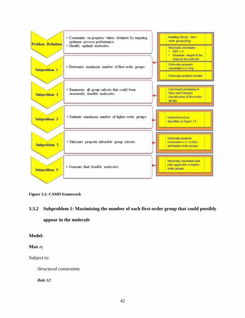
42
Figure 3.2: CAMD framework
3.3.2 Subproblem 1: Maximizing the number of each first-order group that could possibly
appear in the molecule
Model:
Max nf
Subject to:
Structural constraints
Rule 12:

43
𝑛𝑓 ≥ 0∀𝑛𝑓 = 1𝑡𝑜𝑁𝑓 3.15
Rule 13:
𝑛𝑟 {
= 0, 𝑛𝑜𝑐𝑦𝑐𝑙𝑖𝑐𝑓𝑟𝑎𝑔𝑚𝑒𝑛𝑡𝑠≥ 3, 𝑐𝑦𝑐𝑙𝑖𝑐𝑓𝑟𝑎𝑔𝑚𝑒𝑛𝑡𝑠𝑒𝑥𝑖𝑠𝑡
𝑛𝑎𝑐 {
= 0, 𝑛𝑜𝑎𝑟𝑜𝑚𝑎𝑡𝑖𝑐𝑓𝑟𝑎𝑔𝑚𝑒𝑛𝑡𝑠= 𝑚𝑢𝑙𝑡𝑖𝑝𝑙𝑒𝑠𝑜𝑓𝑠𝑖𝑥, 𝑝𝑜𝑙𝑦𝑟𝑖𝑛𝑔𝑎𝑟𝑜𝑚𝑎𝑡𝑖𝑐𝑓𝑟𝑎𝑔𝑚𝑒𝑛𝑡𝑠𝑒𝑥𝑖𝑠𝑡
≥ 10, 𝑓𝑢𝑠𝑒𝑑𝑎𝑟𝑜𝑚𝑎𝑡𝑖𝑐𝑓𝑟𝑎𝑔𝑚𝑒𝑛𝑡𝑠𝑒𝑥𝑖𝑠𝑡
3.16
Rule 11:
𝐹𝐵𝑁 =∑𝑛𝑓
𝑁𝑓
𝑓=1
𝐹𝐵𝑁𝑓 − 2 [(∑(𝑛𝑓)
𝑁𝑓
𝑓=1
− 1) + 𝑁𝑟𝑖𝑛𝑔𝑠 + 𝑁𝑑] = 0 3.17
Here the problem needs to be solved differently for each specified set of Nrings and Nd.
Additionally, to constrain the length of the chains that the current group contribution model
by Gani et al. (1991) can handle
∑𝑛𝑓
𝑁𝑓
𝑓=0
≤ 12∀𝑛𝑓 = 1𝑡𝑜𝑁𝑓 3.18
Rule 15
𝑓𝑀(𝑃𝑘𝐿) ≤ 𝑓𝑀(𝑃𝑘) ≤ 𝑓𝑀(𝑃𝑘
𝑈)∀𝑏𝑜𝑢𝑛𝑑𝑒𝑑𝑝𝑟𝑜𝑝𝑒𝑟𝑡𝑖𝑒𝑠
𝑓𝑀(𝑃𝑚) = 𝑓𝑀(𝑃𝑚
𝑔𝑜𝑎𝑙)∀𝑝𝑟𝑜𝑝𝑒𝑟𝑡𝑖𝑒𝑠𝑤𝑖𝑡ℎ𝑔𝑜𝑎𝑙𝑣𝑎𝑙𝑢𝑒𝑠
3.19
where, 𝑃𝑘 is calculated using Equations 2.12 & 3.8.
The model is linear in nature and can be globally solved using Microsoft Excel 2007 - Solver based
on the Simplex solution method. The model is fed to the system using Microsoft Excel 2007 -
Visual Basic for Applications (VBA). It is also obvious that the minimum number of each group
is zero.

44
3.3.3 Subproblem 2: Enumerating all group subsets of available first-order groups that
could form at least one molecule
A group subset is a set of distinct objects with length equal to the number of first-order groups
considered and with each object being the numbers of each first order group, f.
For example, consider the first-order groups: CH3, CH2, CH and OH, an example of a group subset
generated is shown in Table 3.3.:
Table 3.3: Example of enumerated group subset.
Group (f) CH3 CH2 CH OH FBN Molecule
Sub group 1 2 1 1 1 0
Subproblem 2 deals with the task of enumerating combinations of all first order groups while
ensuring these combinations are constrained by Rule 11 and Rule 16.
Rule 11 as given by Equation 3.17 ensures the FBN of all group subsets as zero. Additionally, the
group subsets are constrained according to Rule 16 for removing non-feasible subsets. The
constraints representing Rule 16 are derived as follows:
The first order groups are classified into four classes and five categories (Gani et al., 1991) as
shown in Table 3.2 and hence,
∑𝑛𝑋𝑋
≤ 𝐶𝑇,𝐿,𝑛𝐿𝑋
𝑋 = {
𝐶𝑎𝑡𝑒𝑔𝑜𝑟𝑦3𝐶𝑎𝑡𝑒𝑔𝑜𝑟𝑦4𝐶𝑎𝑡𝑒𝑔𝑜𝑟𝑦5
𝐶𝑎𝑡𝑒𝑔𝑜𝑟𝑦3 + 4 + 5𝐶𝑎𝑡𝑒𝑔𝑜𝑟𝑦4 + 5
3.20

45
where, nX is the number of groups in category X; L is the largest possible class; nL is number of
groups in class L; T, the total number of first order groups in a generated group subset is given by:
𝑇 =∑𝑛𝑓
𝑁𝑓
𝑓=0
3.21
and 𝐶𝑇,𝐿,𝑛𝐿𝑋 is the maximum allowable number of groups from category X as given in Equation 3.21
and these limits are given in Appendix A.
Subproblem 2 is an enumeration problem while the solutions are also subject to a few constraints.
The task is performed in Microsoft Excel 2007 with the code being fed to the system using
Microsoft Excel 2007 - Visual Basic for Applications (VBA). Hence the solution to subproblem 2
yields group subsets that could possibly form at least one structurally and functionally feasible
molecule.
3.3.4 Subproblem 3: Estimating possible higher order groups
Earlier methods (Chemmangattuvalappil et al., 2009; Eljack & Eden, 2008) either did not
incorporate the contribution of higher order groups or did not efficiently incorporate higher-order
groups within the algorithm during the initial stage thus carrying a number of infeasible group
subsets until the last stage of molecular design. Incorporating higher order groups at a later stage
in the algorithm may also lead to a situation where some potential combinations are omitted
without being considered in further stages of the algorithm. Algebraically enumerating higher
order groups beforehand would be an efficient extension to these methods, particularly for large
problems that normally are prone to combinatorial explosion.
From Rule 7 and Rule 9, it is evident that higher order groups are built from first order groups and
they overlap with each other. Additionally, owing to the knowledge of the connection between the

46
first order groups forming higher order groups, available free bonds in a higher order group and
possible maximum occurrence of a first order group in a molecule, an algebraic expression can be
generated to estimate the upper bound on the possible occurrence of a given higher order group in
a molecule.
Rule 7 leads to the following expression for identifying the possible number of maximum groups;
if (k : n) is the set of first order groups that are the building blocks of one higher order group, h,
then (nk : nn) is the number of those first order groups present in the molecule, η is the number of
occurrences of one particular first order group in a selected higher order group, nh is the number
of possible higher order groups from those first order groups, then according to
Chemmangattuvalappil et al. (2009):
𝑛ℎ = 𝑀𝑖𝑛 (
𝑛𝑘𝜂𝑘:𝑛𝑛𝜂𝑛) 3.22
According to Rule 7, for instance, to form the higher order group CH (CH3) CH (CH3), there must
be two CH and two (CH3) groups. It is not possible to consider a CH (CH3) group as half of a
higher order group. Hence, nh must be rounded down to the nearest integer number.
Moreover, according to Rule 9, two higher order groups of the same kind can even share first order
groups just like higher order groups of different kind. For instance, 2 OH and 1 CH group can form
2CHOH groups. Hence, possibility of the sharing of available first order groups participating in
the given higher order group is considered. To account for these additions, Equation 3.22 needs to
be corrected depending on the nature of higher order groups if nh > 0. Upper bounds on the possible
existence of higher-order groups are achieved by identifying closely connected confirmations of
their respective building blocks and counting the higher-order groups in that confirmation. Also,
while identifying these confirmations, it is ensured that the free bonds of each involved first-order

47
group are maximally utilized. Once this is identified, the correction factors to Equation 3.22 are
carefully explored for respective higher order groups.
For example, in the higher-order group, CH (CH3) CH (CH3), Equation 3.22 becomes:
𝑛ℎ = 𝑀𝑖𝑛 (
𝑛𝐶𝐻2:𝑛𝐶𝐻32) 3.23
But on account of the possibility of sharing of first-order groups, the upper bound of its existence
in a molecule is possible by the closely connected sequential confirmation of first order groups
CH3 and CH as -CH (CH3) CH (CH3) CH (CH3) CH (CH3)-
The correction to Equation 3.22 can now be given by the equation set in Equation 3.24.
𝑘 = 𝑀𝑖𝑛 (
𝑛𝐶𝐻1:𝑛𝐶𝐻31) 𝑎𝑛𝑑
𝑛ℎ = 𝑘 − 1
3.24

48
Figure 3.3: Method to estimate maximum number of higher-order groups.
3.3.5 Subproblem 4: Eliminating property infeasible group subsets
The property Pk of a molecule can be estimated using equation 2.12. The contribution towards a
property Pk from the higher order groups in each group subset obtained in subproblem 2 is not a
unique value. It fluctuates between an upper and lower bound as the different confirmations of
first-order groups in each group subset may lead to formation of different higher order groups. The
maximum and minimum of this value is obtained by solving the following linear model for each
group subset.

49
Max∑𝑛ℎ𝑃𝑘,ℎ
𝑁ℎ
ℎ=1
Subject to:
0 ≤ 𝑛ℎ ≤ 𝑛ℎ𝑚𝑎𝑥 3.25
Where, 𝑛ℎ𝑚𝑎𝑥 is obtained from subproblem 3 for each higher order group and 𝑃𝑘,ℎ is taken from
Marrero and Gani (2001)
Once the maximum and minimum property values for each group subsets are known, the
group subsets are checked against the property constraints given by Equation 3.19. If the estimated
property range of a group subset falls completely outside the targeted property range of molecules,
the group subset is excluded from being considered further.
3.3.6 Subproblem 5: Forming final molecules.
First, all possible combinations of higher order groups for each group subset capable of forming
structurally and functionally feasible molecule are enumerated. This ensures the identification of
structural isomers as the possibility of nonexistence of each higher order groups is considered
which in turn leads to different confirmations of first order groups. As the number of higher order
groups are estimated by considering that all its building first order blocks are used by it alone and
that since these higher order groups overlap with each other, some of the enumerated combinations
can be excluded prior to calculation of their properties. For example: From first order groups 2C,
4CH3, the number of possible higher order groups estimated are n[C(CH3)(CH3)C(CH3)(CH3)] =
1 and n[C(CH3)(CH3) (CH3)]=1. It is clearly seen that both these higher order groups cannot
coexist because for these higher order confirmations to coexist the minimum number of CH3
groups needed is 5. Again Rule 10 indicates that a higher order group is not completely overlapped

50
by any other higher order group. Hence, the combinations which could form a molecule only by
allowing a complete overlap of higher-order groups are also eliminated. Finally, for the remaining
combinations of first- and higher-order groups, if the combination of the groups forms possible
molecules satisfying all structural constraints without any floating free bonds, knowing the number
of existing first order and higher order groups in each enumerated combination, the property of the
molecule is calculated by Equations 3.7 & 3.8. Finally, the feasibility of all designed molecules
with respect to their properties is checked. This is done by checking if all the property constraints
from the process targeting model are met.
3.4 Summary
This chapter covers techniques to solve product design problems from a property platform.
Molecular design by a decomposition approach using Marrero and Gani (2001) GC groups is
discussed. In cases where the property contributions of groups are not available in literature, the
contribution is estimated using a CI based property model. The method developed in this
dissertation is a “generate and test” method, but taking into account the higher order groups and
handling them efficiently, the developed method does not suffer from combinatorial explosion –
an inherent drawback of conventional generate and test methods.
3.5 Case Studies – Computer Aided Molecular Design
3.5.1 Case Study – Design of blanket wash solvent
The application of the developed approach for product design is illustrated by reworking the design
of a blanket wash solvent for a phenolic resin printing ink. Sinha and Achenie (2001) originally
solved this design as a mixed-integer non-linear programming problem (MINLP). Eljack and Eden

51
(2008) solved the problem visually using molecular property clusters. An algebraic molecular
design approach using higher order groups has been developed by Chemmangattuvalappil et al.
(2009) but its application range could be improved if the accuracy of the property prediction is
enhanced by the improved techniques for enumerating higher order groups developed in this
dissertation. The method aims at removing most of the infeasible combinations of groups capable
of forming molecules before the final molecules can be further considered for experimental tests.
Also, this new method is significantly less computationally intensive compared to the previous
geometric and non-linear programming methods of molecular design.
Problem Statement:
Solvents are extensively used as a major component of ink in the printing industry. In letterpress
and offset lithographic printing processes, the inked image on a printing plate is printed on a
rubber cylinder commonly known as “blankets” and then transferred to paper or other material.
The produced quality images are greatly dependent on the cleanliness of the blanket. Paper fibers,
ink residue, paper coating and dried ink etc. must be removed from the rubber blankets. Blanket
washes are specially formulated to clean ink and other residues from rubber blankets. They are
generally petroleum-based solvents that consist of volatile organic compounds (VOCs).
Reasonably, there is a lot of concern regarding the effects of such solvents on the environment as
well as the direct effect on human health.
The goal of this study is to design optimal solvents to be used as a blanket wash. These solvents
should (a) have minimal drying time (b) be liquid at room temperature (c) have low vapor pressure
(VP), and (d) dissolve the ink. Hence, solubility (Rij) of the solvent is an important factor, the
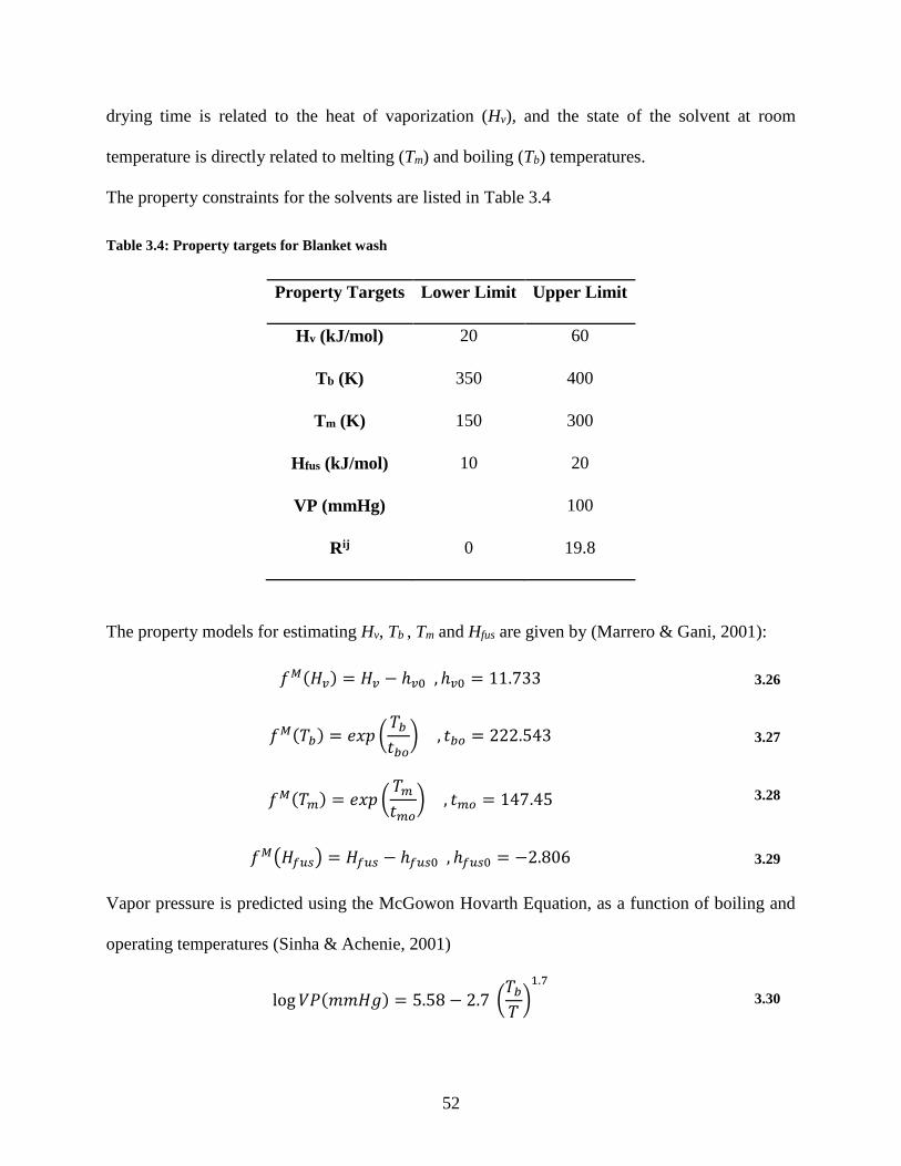
52
drying time is related to the heat of vaporization (Hv), and the state of the solvent at room
temperature is directly related to melting (Tm) and boiling (Tb) temperatures.
The property constraints for the solvents are listed in Table 3.4
Table 3.4: Property targets for Blanket wash
Property Targets Lower Limit Upper Limit
Hv (kJ/mol) 20 60
Tb (K) 350 400
Tm (K) 150 300
Hfus (kJ/mol) 10 20
VP (mmHg) 100
Rij 0 19.8
The property models for estimating Hv, Tb , Tm and Hfus are given by (Marrero & Gani, 2001):
𝑓𝑀(𝐻𝑣) = 𝐻𝑣 − ℎ𝑣0, ℎ𝑣0 = 11.733 3.26
𝑓𝑀(𝑇𝑏) = 𝑒𝑥𝑝 (
𝑇𝑏𝑡𝑏𝑜) , 𝑡𝑏𝑜 = 222.543 3.27
𝑓𝑀(𝑇𝑚) = 𝑒𝑥𝑝 (
𝑇𝑚𝑡𝑚𝑜
) , 𝑡𝑚𝑜 = 147.45 3.28
𝑓𝑀(𝐻𝑓𝑢𝑠) = 𝐻𝑓𝑢𝑠 − ℎ𝑓𝑢𝑠0, ℎ𝑓𝑢𝑠0 = −2.806 3.29
Vapor pressure is predicted using the McGowon Hovarth Equation, as a function of boiling and
operating temperatures (Sinha & Achenie, 2001)
log 𝑉𝑃(𝑚𝑚𝐻𝑔) = 5.58 − 2.7 (
𝑇𝑏𝑇)1.7
3.30

53
The effectiveness of the designed solvent is greatly dependent on its ability to dissolve the ink, i.e.
it is dependent on the solubility power of the designed solvent. The interactions between phenolic
resin molecules (solute) with the solvent molecules are very important in this design problem.
Solubility, Rij is determined by using (Sinha & Achenie, 2001):
𝑅𝑖𝑗 = √4(𝛿𝑑𝑖 − 𝛿𝑑𝑗)2 + (𝛿𝑝𝑖 − 𝛿𝑝𝑗)2 + (𝛿ℎ𝑖 − 𝛿ℎ𝑗)2 3.31
where i correspond to the solvent while j corresponds to the solute and each 𝛿 parameter can be
estimated using the following equations (Van Krevelen and Hoftyzer, 1976):
𝛿𝑑 =
∑ 𝐹𝑑𝑖𝑖
𝑉 𝛿𝑝 =
∑ 𝐹𝑝𝑖2
𝑖
𝑉 𝛿ℎ =
∑ 𝐸ℎ𝑖𝑖
𝑉 3.32
where Fd is the dispersion component, Fp the polar component and Eh the contribution of hydrogen
bonding forces. These parameters can also be calculated by the group contribution method
proposed by Pistikopoulos and Stefanis (1998).
Phenolic resins are commonly used in printing inks. The dried ink (solute) is assumed to be
phenolic resins, specifically ‘Super Bakacite® 1001, Reichhold’. The solubility parameter
components of the resin are non-polar, δdj= 23.3, polar, δpj = 6.6 and hydrogen bonding, δhj=
8.3 MPa1/2 (Barton, 1985). The molecular property targets based on Equations 3.26- 3.29 is given
in Table 3.5.
Table 3.5: Molecular property targets for blanket wash.
Molecular Property Targets Lower Limit Upper Limit
Hv (kJ/mol) 8.268 48.268
Tb (K) 4.8195 6.034

54
Tm (K) 2.7657 7.6489
Hfus (kJ/mol) 12.806 22.806
The following first order groups have been considered for molecular design:
1 CH3 5 CH-O
2 CH2 6 CH3-CO
3 CH 7 CH2-CO
4 OH
Subproblem 1:
Property data for these selected groups is taken from Marrero and Gani (2001), which are
reproduced in Appendix A. Now, inequality expressions for each property are formulated. The
number of preselected first order molecular groups is maximized subject to the specific constraints
mentioned in Table 3.5. The reason behind maximizing these groups is to ensure that no potential
molecule is left out. The variations in the property values caused by inclusion of the higher order
groups will be considered in the later stages.
The maximum values are as follows:
max max
CH3 3 CH-O 2
CH2 6 CH3-CO 1

55
CH 2 CH2-CO 1
OH 1
Subproblem 2:
The class and category of the groups considered above are obtained from the group classification
tables by Gani et al. (1991).
Group Class Category
CH3 1 1
CH2 2 1
CH 3 1
OH 1 4
CH-O 1 4
CH3-CO 1 3
CH2-CO 2 3
350 group subsets whose FBN is zero are generated. For each of these subsets, the number of
groups, nX in each of category X such that X= 3, 4, 5, 3+4+5, 4+5, is identified and checked
against 𝐶𝑇,𝐿,𝑛𝐿𝑋 such that:
∑𝑛𝑋𝑋
≤ 𝐶𝑇,𝐿,𝑛𝐿𝑋 3.33
where, L is the largest possible class; nL is the number of groups in class L; T is the total number
of first order groups in the group subset and 𝐶𝑇,𝐿,𝑛𝐿𝑋 is identified using Table A.15 .

56
269 of the tested group subsets satisfy the class and category constraints and these are considered
for further subproblems.
Subproblem 3:
The possible higher-order groups are identified in Table 3.6.
Table 3.6: Possible higher order groups for blanket wash case study.
1 (CH3)2CH
2 CH(CH3)CH(CH3)
3 CH-CHO
4 CH2-CH3CO
5 CH-CH3CO
6 CHOH
7 OH-CH-CH3CO
8 OH-CH2-CH3CO
The maximum possible number of each higher-group is computed algebraically by using the
methodology explained in the previous chapter as shown below.
1. (CH3)2CH
If the group subsets comprises of only 3 CH3 and 1CH groups,𝑛ℎ = 2;
Else, 𝑛ℎ = 𝑖𝑛𝑡 (min (𝑛𝐶𝐻3
2; 𝑛𝐶𝐻))
2. CH(CH3)CH(CH3)
Maximum number of groups of this kind can exist when the groups CH(CH3) are
positioned in a series, Hence, if a is the number of CH(CH3) groups i.e.,

57
𝐼𝑓𝑎 = 𝑖𝑛𝑡(min(𝑛𝐶𝐻3; 𝑛𝐶𝐻))𝑎𝑛𝑑𝑎 > 1;
𝑛ℎ = 𝑎 − 1𝐸𝑙𝑠𝑒𝑛ℎ = 0
3. CH-CHO
If a is the number of CH(CHO)2 groups, b is the number of CH-CHO groups from balance
CH and CHO groups, i.e.
𝐼𝑓𝑎 = 𝑖𝑛𝑡 (min (𝑛𝐶𝐻𝑂2
; 𝑛𝐶𝐻)) 𝑎𝑛𝑑𝑏 = 𝑖𝑛𝑡(min(𝑛𝐶𝐻𝑂; 𝑛𝐶𝐻))
𝑛ℎ = 2𝑎 + 𝑏
4. CH2-CH3CO
If the group subsets comprises of only 2 CH3CO and 1CH2 groups,𝑛ℎ = 2;
Else, 𝑛ℎ = 𝑖𝑛𝑡(min(𝑛𝐶𝐻3𝐶𝑂; 𝑛𝐶𝐻2))
5. CH- CH3CO
If a is the number of CH(CH3CO)2 groups, b is the number of CH- CH3CO groups from
balance CH and CH3CO groups, i.e.
𝐼𝑓𝑎 = 𝑖𝑛𝑡 (min (𝑛𝐶𝐻3𝐶𝑂
2; 𝑛𝐶𝐻)) 𝑎𝑛𝑑𝑏 = 𝑖𝑛𝑡(min(𝑛𝐶𝐻3𝐶𝑂; 𝑛𝐶𝐻))
𝑛ℎ = 2𝑎 + 𝑏
6. CHOH
If a is the number of CH(OH)2 groups, b is the number of CHOH groups from balance CH
and OH groups, i.e.
𝐼𝑓𝑎 = 𝑖𝑛𝑡 (min (𝑛𝑂𝐻2; 𝑛𝐶𝐻)) 𝑎𝑛𝑑𝑏 = 𝑖𝑛𝑡(min(𝑛𝑂𝐻; 𝑛𝐶𝐻))
𝑛ℎ = 2𝑎 + 𝑏
7. OH-CH-CH3CO

58
If the group subsets comprises of 1 CH and total of 3 [OH + CH3CO] groups alone 𝑛ℎ =
1;
Else, 𝑛ℎ = 𝑖𝑛𝑡(min(𝑛𝐶𝐻3𝐶𝑂; 𝑛𝐶𝐻; 𝑛𝑂𝐻))
8. OH-CH2-CH3CO
It is whole molecule, so, if the group subsets comprise of 1 CH2 and total of 1 OH and 1
CH3CO groups alone𝑛ℎ = 1;
Subproblem 4:
For each group subset to be tested in this subproblem, the maximum and minimum contributions
from possible higher-order groups are estimated. Based on the molecular property constraints
listed in Table 3.5, group subsets whose property range falls completely outside the targeted
property range of molecules are excluded from being considered further. 18 group subsets obey
the property constraints and are hence considered for the next subproblem.
Subproblem 5:
All possible combinations of higher order groups for each group subset capable of forming
structurally and functionally feasible molecule are enumerated. 42 group subsets have been
identified and checked if a molecule with targeted properties is possible from those subsets. The
molecules identified by solving molecular design model are listed below in Table 3.7.
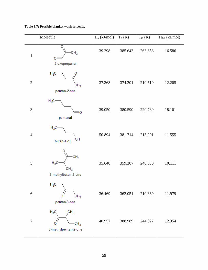
59
Table 3.7: Possible blanket wash solvents.
Molecule Hv (kJ/mol) Tb (K) Tm (K) Hfus (kJ/mol)
1
39.298
385.643
263.653
16.586
2
37.368 374.201 210.510 12.205
3
39.050 380.590 220.789 18.101
4
50.894 381.714 213.001 11.555
5
35.648 359.287 248.030 10.111
6
36.469 362.051 210.369 11.979
7
40.957 388.989 244.027 12.354

60
8
40.238 391.122 226.134 11.756
9
37.010 368.624 227.685 15.013
10
36.859 363.247 201.392 14.248
11
41.379 391.275 219.031 14.618
12
41.920 397.049 235.412 17.652
13
41.769 392.324 210.581 16.887
14
42.319 397.180 223.081 17.256

61
15
53.764 398.093 228.376 11.106
16
53.957 387.465 193.351 10.111
17
54.163 398.223 215.415 10.710
18
41.627 398.074 157.093 16.348
19
39.339 379.885 226.007 11.530
20
39.738 380.026 212.826 11.134
21
39.587 387.035 167.584 13.260

62
22
40.261 393.333 245.513 12.033
Vapor pressure (VP), and solubility (Rij) of the solvent are calculated for the above solvents and
listed in the following Table 3.8.
Table 3.8: Vapor pressure and solubility calculations for identified blanket wash solvents.
Molecule VP (mmHg) Solubility
1 2-oxopropanal 24.822 15.047
2 pentan-2-one 40.154 15.087
3 pentanal 30.735 15.113
4 butan-1-ol 29.313 15.542
5 3-methylbutan-2-one 74.022 15.638
6 pentan-3-one 66.176 14.886
7 3-methylpentan-2-one 21.523 15.779
8 4-methylpentan-2-one 19.645 15.779
9 3-methylbutanal 50.577 15.636
10 2-methylbutanal 63.035 15.636
11 hexan-3-one 19.516 15.007
12 4-methylpentanal 15.213 15.734
13 2-methylpentanal 18.656 15.734

63
14 3-methylpentanal 15.127 15.734
15 3-methylbutan-1-ol 14.539 15.999
16 pentan-2-ol 22.970 15.992
17 2-methylbutan-1-ol 14.457 15.992
18 octane 14.551 17.297
19 2-methylpentan-3-one 31.660 15.564
20 4-methylhexan-3-one 31.473 15.564
21 2-methylheptane 23.394 17.946
22 2-3-dimethylbutanal 17.863 16.279
Since all the molecules found by solving the molecular design satisfy the property target limits for
vapor pressure and solubility, they can be considered for further tests like experimentation or other
property checks. Molecules 1, 2, 3, 4, 6, 7, 10, 21, and 22 are the ones identified by
Chemmangattuvalappil et al. (2009) The other molecules identified in that work are excluded due
the feasibility constraints applied in subproblem 2. For example, the 2-Hydroxypropanol molecule
has OH and CHO groups on the same carbon and hence is likely to be unstable as a solvent. By
applying feasibility constraints based on class and category classification of first-order groups,
such infeasible molecules can be excluded. Also, the methodology developed here identifies the
possible structural isomers as the possibility of nonexistence of each higher order group is
considered while generating the combination of groups. Pentan-3-one identified by Sinha and
Achenie (2001) is identified using current methodology, the other two namely propanol and
methyl-ethyl ketone were not identified owing to the change in selection of property targets. Due

64
to the usage of algebraic approaches in the developed methodology, it generated the feasible
structures more efficiently than the visual approach by Eljack and Eden (2008).
3.5.2 Case Study – Design of cyclic molecules
A general problem is considered to illustrate the capability of the developed molecular design
methodology for generating cyclic molecules.
The property constraints for the solvents are listed in Table 3.9.
Table 3.9: Property targets for cyclic molecules.
Property Targets Lower Limit Upper Limit
Hv (kJ/mol) 20 60
Tb (K) 350 400
Tm (K) 150 300
Hfus (kJ/mol) 10 20
The property models for estimating Hv, Tb , Tm and Hfus are given by (Marrero & Gani, 2001):
𝑓𝑀(𝐻𝑣) = 𝐻𝑣 − ℎ𝑣0, ℎ𝑣0 = 11.733 3.34
𝑓𝑀(𝑇𝑏) = 𝑒𝑥𝑝 (
𝑇𝑏𝑡𝑏𝑜) , 𝑡𝑏𝑜 = 222.543 3.35
𝑓𝑀(𝑇𝑚) = 𝑒𝑥𝑝 (
𝑇𝑚𝑡𝑚𝑜
) , 𝑡𝑚𝑜 = 147.45 3.36
𝑓𝑀(𝐻𝑓𝑢𝑠) = 𝐻𝑓𝑢𝑠 − ℎ𝑓𝑢𝑠0, ℎ𝑓𝑢𝑠0 = −2.806 3.37
The molecular property targets based on Equations 3.34 - 3.37 is given in Table 3.10.

65
Table 3.10: Molecular property targets for cyclic molecules.
Molecular Property Targets Lower Limit Upper Limit
Hv (kJ/mol) 8.268 48.268
Tb (K) 4.8195 6.034
Tm (K) 2.7657 7.6489
Hfus (kJ/mol) 12.806 22.806
The following first order groups have been considered for molecular design:
1 CH3 5 CH-O
2 CH2 6 CH2 (ring)
3 CH 7 CH (ring)
4 OH
Subproblem 1:
The maximum values of each first-order group selected are as follows:
max max
CH3 4 CH-O 1
CH2 4 CH2 (ring) 3
CH 1 CH (ring) 4
OH 0
This shows that molecules with OH functional group do not possess the required properties.

66
Subproblem 2:
The class and category of the groups considered above are obtained from the group classification
tables by Gani et al. (1991).
Group Class Category
CH3 1 1
CH2 2 1
CH 3 1
OH 1 4
CH-O 1 4
CH2 (ring) 2 1
CH (ring) 3 1
187 group subsets whose FBN is zero are generated. FBN here is calculated using the following
equation. The number of rings is pre-specified to be 1.
𝐹𝐵𝑁 =∑𝑛𝑓
𝑁𝑓
𝑓=1
𝐹𝐵𝑁𝑓 − 2 [(∑(𝑛𝑓)
𝑁𝑓
𝑓=1
− 1) + 𝑁𝑟𝑖𝑛𝑔𝑠] = 0 3.38
For each of these subsets, the number of groups, nX in each category X such that X= 3, 4, 5, 3+4+5,
4+5, is identified and checked against 𝐶𝑇,𝐿,𝑛𝐿𝑋 such that:
∑𝑛𝑋𝑋
≤ 𝐶𝑇,𝐿,𝑛𝐿𝑋 3.39
where, L is the largest possible class; nL is number of groups in class L; T is the total number of
first order groups in the group subset and 𝐶𝑇,𝐿,𝑛𝐿𝑋 is identified using Table A.17.All 187 group

67
subsets satisfy constraints pertaining to class and category of the groups and hence all of them are
considered for further subproblems.
Subproblem 3:
The possible higher-order groups are identified in Table 3.11.
Table 3.11: Possible higher order groups for cyclic molecules.
1 (CH3)2CH
2 CH(CH3)CH(CH3)
3 CH-CHO
4 CHcyc-CH3
5 CHcyc-CH2
6 CHcyc-CH
7 CHcyc-CHO
The maximum possible number of each higher-group is computed algebraically by using the
methodology explained. The method to calculate the maximum number of each of groups 1-3 in
Table 3.11 was explained in subproblem 3 of case study 1. Groups 4-7 can be generally represented
as CHcyc-A as CHcyc has 3 free bonds and two of these are involved in bonding to only cyclic first-
order groups and only one free bond is available for their respective non-cyclic first order groups.
Hence, the maximum of these groups can be calculated by:
𝑛ℎ = 𝑖𝑛𝑡 (min (𝑛𝐶𝐻𝑐𝑦𝑐; 𝑛𝐴))
Subproblem 4:
For each of group subset to be tested in this subproblem, the maximum and minimum contributions
from possible higher-order groups are estimated. Based on the molecular property constraints

68
listed in Table 3.10, group subsets whose property range falls completely outside the targeted
property range of molecules are excluded from being considered further. 15 group subsets obey
the property constraints and are hence considered for the next subproblem.
Subproblem 5:
All possible combinations of higher order groups for each group subset capable of forming
structurally and functionally feasible molecule are enumerated. Additionally, for group subsets
containing both cyclic and acyclic first-order groups, another constraint to check if cyclic groups
(after forming a ring) can accommodate acyclic groups to form a molecule. 64 group subsets have
been identified and checked if a molecule with targeted properties is possible from those subsets.
The molecules identified by solving the molecular design model are listed below in Table 3.12.
Table 3.12: Possible cyclic molecules.
S.
No
Molecule
Hv
(kJ/mol)
Tb (K) Tm (K)
Hfus
(kJ/mol)
1
40.542 372.5846 245.0608 14.242
2
41.683 378.5528 203.5736 14.675

69
3
45.024 409.7074 223.318 15.744
4
46.593 405.8108 212.6318 17.314
5
40.589 358.6316 228.9984 16.308
6
43.93 392.4921 245.7865 17.377
7
44.983 396.2557 229.1574 17.029
8
44.975 392.37 226.408 17.777

70
9
45.071 397.9558 204.5344 17.81
10
43.977 379.7679 229.8074 19.443
11
39.663 399.3066 166.4824 10.262
12
38.602 383.9691 158.3832 11.944
Molecules 3 and 4 have properties outside of the targeted range and hence are eliminated from
the list of valid molecules.

71
4. Property Based Process Design and its Integration with Molecular Design
4.1 Property Operators and Clustering Techniques
Standard process design techniques are chemo-centric in nature, i.e. they are based on tracking,
manipulation, and allocation of individual chemical species. But, many processes are driven and
governed by properties or functionalities of the streams and not by their chemical constituency.
For instance, the usage of material utilities (e.g. solvents) relies on their characteristics, such as
equilibrium distribution coefficients, viscosity, and volatility without the need to chemically
characterize these materials. Constraints on process units that can accept recycled/reused process
streams and wastes are not limited to compositions of components but are also based on the
properties of the feeds to processing units (El-Halwagi, 2006). In the design of paper with a
specified quality, the quality is specified in terms of the physical properties and not in terms of
components as the basic component of all types of paper is cellulose (Eden et al., 2004). Since
properties (or functionalities) form the basis of performance for many processes, design procedures
based on key properties instead of key compounds are needed. But, unlike mass, properties are not
conserved and cannot be tracked among units without undertaking component material balances.
Therefore, to resolve these limitations, property-based clusters which are conserved are used
(Shelley & El-Halwagi, 2000). The property clusters are formed based on property operators,
which are functions of actual physical properties that obey linear additive rules (Eden et al., 2004;
Shelley & El-Halwagi, 2000).

72
For a mixture made up of Ns streams and described by j properties, the property operator, Ψj(PjM)
corresponding to the property P is formulated as follows:
𝛹𝑗(𝑃𝑗𝑀) =∑𝑥𝑠 ⋅ 𝛹𝑗(𝑃𝑗𝑠)
𝑁𝑠
𝑠=1
4.1
Here, Ψj (Pjs) is the operator of the jth property Pjs of stream s and xs is the fractional contribution
given by
𝑥𝑠 =
𝐹
∑ 𝐹𝑠𝑁𝑠𝑠=1
4.2
The property operators can be evaluated from first principles or estimated through empirical or
semi-empirical methods. Density for instance, where the resulting property of mixing two streams
is given as the inverse of the summation over the reciprocal property values multiplied by their
fractional contribution xs as shown below
1
𝜌𝑀=∑𝑥𝑠
𝑁𝑠
𝑠=1
⋅1
𝜌𝑠 𝛹𝑗(𝑃𝑗𝑀) =
1
𝜌𝑀 𝛹𝑗(𝑃𝑗𝑠) =
1
𝜌𝑠 4.3
The properties involved in the system are of different units and magnitudes. So, the operators are
normalized into a dimensionless form by dividing with an appropriately chosen reference operator.
The normalized property operator is given as:
𝛺𝑗𝑠 =
𝛹𝑗𝑠(𝑃𝑗𝑠)
𝛹𝑗𝑠(𝑃𝑗𝑟𝑒𝑓) 4.4
An Augmented Property index AUP for each stream s is the sum of all the NP dimensionless
property operators:
𝐴𝑈𝑃𝑠 =∑𝛺𝑗𝑠
𝑁𝑃
𝑗=1
4.5
Finally, the property cluster Cjs for property j is defined as:

73
𝐶𝑗𝑠 =
𝛺𝑗𝑠
𝐴𝑈𝑃𝑠 4.6
These clusters, in a way, give the contribution of each property to its respective targeted value.
Clusters enable the conserved tracking of properties and the derivation of visualization design
tools. Also, these clusters possess two characteristics: intra- and inter-stream conservation (Eden
et al., 2004). Figure 4.1 shows the ternary representation of these characteristics.
4.1.1 Intra-Stream Conservation
For any stream s, the sum of clusters corresponding to Nc properties is constant and adds up to
unity, i.e.
∑𝐶𝑗𝑠 = 1
𝑁𝑐
𝑗=1
4.7
Figure 4.1: Ternary representation of clusters and their intra- and inter-stream conservation characteristics.

74
Two points 𝐶𝑗𝑠1(𝐶1𝑠1,𝐶2𝑠1,𝐶3𝑠1) and 𝐶𝑗𝑠2(𝐶1𝑠2,𝐶2𝑠2,𝐶3𝑠2) are seen to be having the sum of their
respective property clusters to be unity. Hence, if (Nc-1) clusters for a stream are given, the Ncth
cluster can be uniquely identified.
4.1.2 Inter-Stream Conservation
For any two or more streams that are mixed, the resulting individual cluster is conserved. Additive
rules in the form of lever-arm rules aid in obtaining the mean cluster property of two or more
mixed streams. The lever-arm rule can be represented by (Eden et al., 2004):
𝐶𝑗𝑀 =∑𝛽𝑠 ⋅ 𝐶𝑗𝑠
𝑁𝑠
𝑠=1
4.8
where CjM is the mean cluster of jth property and s represents the fractional lever arm of cluster,
Cjs, of stream s. The cluster arm is given by:
𝛽𝑠 =
𝑥𝑠 ⋅ 𝐴𝑈𝑃𝑠𝐴𝑈𝑃𝑀
4.9
and also
∑𝛽𝑠 = 1
𝑁𝑠
𝑠=1
4.10
Indicating
𝐴𝑈𝑃𝑀 =∑𝑥𝑠⋅
𝑁𝑠
𝑠=1
𝐴𝑈𝑃𝑠 4.11
Using AUP in the lever-arm rule enables one-to-one mapping from raw properties to property
clusters and vice versa when streams are mixed (El-Halwagi, 2006). Hence, if clusters of (Ns-1)
streams are given, owing to the inter-stream conservation property, the Nsth clusters can be

75
uniquely found. Also the mixture cluster of two streams will lie on a straight line connecting those
two points.
4.2 Process Design by Visualization tools
The objective here is to develop visualization tools that systematically minimize usage of fresh
resources and maximize utilization of process resources into a process sink along with
identification of the fresh resource’s feasibility region and the corresponding property targets
without committing to any components in the fresh source (until the final step).
4.2.1 Identification of feasibility region for sink
The geometric shape of the feasibility region for each sink (units capable of processing the sources)
has to be identified first in order to address the above mentioned problem. Constructing the
boundaries of the feasibility region (BFR) for the sink is not that straightforward and hence needs
definite construction rules (El-Halwagi, Glasgow, Qin, & Eden, 2004)
Consider a sink with three targeted properties, each of them being bounded by a lower and upper
limit.
𝑃𝑗,𝑠𝑖𝑛𝑘𝑚𝑖𝑛 ≤ 𝑃𝑗 ≤ 𝑃𝑗,𝑠𝑖𝑛𝑘
𝑚𝑎𝑥 →Ω𝑗,𝑠𝑖𝑛𝑘𝑚𝑖𝑛 ≤ Ω𝑗 ≤ Ω𝑗,𝑠𝑖𝑛𝑘
𝑚𝑎𝑥 4.12
Based on Equation 4.12, the rules developed by El-Halwagi et al. (2004) for a system involving
three properties are summarized below.
Rule 17: The BFR is accurately represented by six line segments.
Rule 18: The extended linear segments of the BFR constitute three convex hulls (cones) with their
heads lying on the three vertices of the ternary cluster diagram.

76
Rule 19: The cluster boundary values defining the BFR are characterized by the following values
of dimensionless operators for the sink constraints.
𝐶1,𝑠𝑖𝑛𝑘𝑚𝑖𝑛 =
Ω1,𝑠𝑖𝑛𝑘𝑚𝑖𝑛
Ω1,𝑠𝑖𝑛𝑘𝑚𝑖𝑛 + Ω2,𝑠𝑖𝑛𝑘
𝑚𝑎𝑥 + Ω3,𝑠𝑖𝑛𝑘𝑚𝑎𝑥
4.13
𝐶1,𝑠𝑖𝑛𝑘𝑚𝑎𝑥 =
Ω1,𝑠𝑖𝑛𝑘𝑚𝑎𝑥
Ω1,𝑠𝑖𝑛𝑘𝑚𝑎𝑥 + Ω2,𝑠𝑖𝑛𝑘
𝑚𝑖𝑛 + Ω3,𝑠𝑖𝑛𝑘𝑚𝑖𝑛
4.14
𝐶2,𝑠𝑖𝑛𝑘𝑚𝑖𝑛 =
Ω2,𝑠𝑖𝑛𝑘𝑚𝑖𝑛
Ω1,𝑠𝑖𝑛𝑘𝑚𝑎𝑥 + Ω2,𝑠𝑖𝑛𝑘
𝑚𝑖𝑛 + Ω3,𝑠𝑖𝑛𝑘𝑚𝑎𝑥
4.15
𝐶2,𝑠𝑖𝑛𝑘𝑚𝑎𝑥 =
Ω2,𝑠𝑖𝑛𝑘𝑚𝑎𝑥
Ω1,𝑠𝑖𝑛𝑘𝑚𝑖𝑛 + Ω2,𝑠𝑖𝑛𝑘
𝑚𝑎𝑥 + Ω3,𝑠𝑖𝑛𝑘𝑚𝑖𝑛
4.16
𝐶3,𝑠𝑖𝑛𝑘𝑚𝑖𝑛 =
Ω3,𝑠𝑖𝑛𝑘𝑚𝑖𝑛
Ω1,𝑠𝑖𝑛𝑘𝑚𝑎𝑥 + Ω2,𝑠𝑖𝑛𝑘
𝑚𝑎𝑥 + Ω3,𝑠𝑖𝑛𝑘𝑚𝑖𝑛
4.17
𝐶3,𝑠𝑖𝑛𝑘𝑚𝑖𝑛 =
Ω3,𝑠𝑖𝑛𝑘𝑚𝑎𝑥
Ω1,𝑠𝑖𝑛𝑘𝑚𝑖𝑛 + Ω2,𝑠𝑖𝑛𝑘
𝑚𝑖𝑛 + Ω3,𝑠𝑖𝑛𝑘𝑚𝑎𝑥
4.18
By simply bounding the region within the minimum and maximum values of the clusters identified
above, the overestimation of the feasibility region is determined. While this boundary guarantees
the existence of feasible points inside it, the true feasible region is obtained by connecting the six
points corresponding to the above six cluster boundary values (each coordinate of whose represent
a property operator value) corresponding to respective boundary clusters. This stems from the fact
that all these points are part of the true feasibility region and that any mixtures of those points must
also lie within the true feasibility region. This is depicted in Figure 4.2 (Eden et al., 2004).

77
Figure 4.2: Boundary Feasible region
4.2.2 Source - Sink Mapping
After the BFR of the sink has been found as illustrated in section 4.2.1, the next step is to map
source streams and/or their mixtures into this sink. The stream or mixture stream is qualified to be
processed by a sink if
The point representing stream clusters is contained within the feasibility region of the sink on
the cluster ternary diagram.
The values of the augmented property index (AUP) for the source (or mixture of sources) and
the sink must match.
The flow rate of the source (or mixture of sources) must lie within the acceptable feed flow
rate range for the sink.
Any cluster point in the ternary diagram corresponds to multiple combinations of property points
due to the nonlinear mapping from the property to cluster domain (Section 4.1).

78
Therefore, having the cluster value inside the sink region alone will not ensure that the properties
are in the correct range. In order to make sure that the properties match the sink requirements, the
AUP values of sink and source streams must also match. Additionally the flow rate of the source,
or mixture of sources, must be within the upper and lower limits of sink’s capacity, otherwise only
a fraction can be recycled.
As all the possible mixture points of two streams lie on a straight line connecting those two points,
if the straight line passes through the sink region, the two streams can be mixed to get the required
stream, Smix, for the sink as shown in Figure 4.3(a).
(a) (b)
Figure 4.3: Source - Sink Mapping
Here S1 and S2 can be mixed to get the optimum output Smix. If Smix1 lies outside the sink’s BFR as
in Figure 4.3(b), another source is added to meet the sink property targets. Sometimes the S1-S2
line may pass through that sink but the mixture point Smix may lie outside the sink BFR. In these
cases, for the mixture to be accepted by the sink, the individual flowrates of S1 and S2 must be
changed.

79
4.2.3 Identification of feasibility region for fresh source
Process constraints based on the sink’s BFR and available source streams in a process are utilized
to design a needed fresh source. Given two available source streams S1 and S2 to be recycled to the
process sink, the source mixture (SM) is identified using the lever-arm principles as shown in
Figure 4.3(b). Owing to the flow rate constraint of the sink, the flow rate of fresh stream is
identified by:
𝐹𝑓𝑟𝑒𝑠ℎ = 𝐹𝑠𝑖𝑛𝑘 −𝐹𝑆𝑀 4.19
In, Figure 4.4, the first feasible region reflects the sink’s original property demands as given by
Equation 4.12. Lever-arm principles are utilized to identify a new feasibility region for the fresh
source. This region serves to integrate the process requirements with the design of fresh source to
be mixed with source mixture.
The feasibility region points (Aꞌ, Bꞌ, Cꞌ, Dꞌ, Eꞌ, Fꞌ) for the fresh stream are determined from point
SM and A, B, C, D, E, F respectively by using Equation 4.20.
For generalization, the line segment connecting points SM and Dꞌ in Figure 4.4 has been magnified
with SM and Dꞌ shown as S1 and S2 respectively in the magnification. D is marked as the mixture
point; the cluster point for Dꞌ is given by:
𝐶𝑗𝑆2 =
𝐶𝑗𝑀 − 𝛽𝑆1𝐶𝑗𝑆1(1 − 𝛽𝑆1)
4.20
Given 𝐶𝑗𝑆1 and 𝐶𝑗𝑀 and calculating 𝛽𝑆1 by Equation 4.9, 𝐶𝑗𝑆2 is determined. Similarly, Aꞌ, Bꞌ, Cꞌ,
Eꞌ, Fꞌ can be easily determined.
Hence, the new property requirements for the fresh source are back calculated from the determined
cluster values while also satisfying the AUP match condition mentioned in section 4.2.2:

80
𝑥𝑆1𝐴𝑈𝑃𝑆1 + (1 − 𝑥𝑆1)𝐴𝑈𝑃𝑆2 = 𝐴𝑈𝑃𝑀 4.21
Figure 4.4: Identification of feasibility region for fresh source (Eljack, Solvason, Chemmangattuvalappil, &
Eden, 2008)
4.3 Process Design by Mathematical Programming
The graphical approach has limitations pertaining to the number of properties it can handle and
also its practicality is inversely proportional to the number of streams and sinks present in the
process. It becomes quite hard to track the properties visually and hence, to overcome these

81
limitations, a mathematical programming formulation is used to address the process design
problem.
Consider a process sink i, 𝑖 = 1,2,3… . . 𝑁𝑠𝑖𝑛𝑘𝑠, The sink’s BFR is defined in terms of j bounded
properties, Pk,𝑘 = 1,2,3… . . 𝑁𝑝𝑟𝑜𝑝𝑒𝑟𝑡𝑖𝑒𝑠 and a permissible flow rate, 𝐹𝑖𝑠𝑖𝑛𝑘. The property bounds
for each sink, i are given by:
𝑃𝑘,𝑖𝐿 ≤ 𝑃𝑘,𝑖 ≤ 𝑃𝑘,𝑖
𝑈 4.22
Since the properties may not be conserved, they are reformulated in terms of their conserved
surrogates by the application of the property operators as mentioned in section 4.1:
[𝛹𝑘(𝑃𝑘,𝑖)]𝐿 ≤ 𝛹𝑘(𝑃𝑘,𝑖) ≤ [𝛹𝑘(𝑃𝑘,𝑖)]
𝑈 4.23
If available source streams j, 𝑗 = 1,2,3… . . 𝑁𝑠𝑜𝑢𝑟𝑐𝑒𝑠 with properties, Pk, j and flow rates,
𝐹𝑖𝑠𝑜𝑢𝑟𝑐𝑒 are to be recycled to the process sinks along with the fresh source, fresh, the process design
problem aims at mathematically finding the admissible property ranges 𝑃𝑘,𝑓𝑟𝑒𝑠ℎ𝑙𝑜𝑤𝑒𝑟 ≤ 𝑃𝑘𝑓,𝑟𝑒𝑠ℎ ≤
𝑃𝑘,𝑓𝑟𝑒𝑠ℎ𝑢𝑝𝑝𝑒𝑟
and flow rate, Ffresh of fresh source into the sinks without committing to any components
in the fresh source.
4.3.1 Mathematical model of the process design problem
Min ±𝛹𝑘(𝑃𝑘,𝑓𝑟𝑒𝑠ℎ)
Subject to:
Flow rate constraints:
𝐹𝑖𝑠𝑖𝑛𝑘 = 𝐹𝑖,𝑓𝑟𝑒𝑠ℎ + ∑ 𝐹𝑖,𝑗
𝑁𝑠𝑜𝑢𝑟𝑐𝑒𝑠
𝑗=1
∀𝑖 = 1𝑡𝑜𝑁𝑠𝑖𝑛𝑘𝑠 4.24

82
𝐹𝑗𝑠𝑜𝑢𝑟𝑐𝑒 = 𝑊𝑗 + ∑ 𝐹𝑖,𝑗
𝑁𝑠𝑖𝑛𝑘𝑠
𝑖=1
∀𝑗 = 1𝑡𝑜𝑁𝑠𝑜𝑢𝑟𝑐𝑒𝑠 4.25
𝐹𝑓𝑟𝑒𝑠ℎ = ∑ (𝐹𝑖𝑠𝑖𝑛𝑘) − ∑ 𝐹𝑖
𝑠𝑜𝑢𝑟𝑐𝑒
𝑁𝑠𝑜𝑢𝑟𝑐𝑒𝑠
𝑖=1
𝑁𝑠𝑖𝑛𝑘𝑠
𝑖=1
; 𝐼𝑓 ∑ 𝐹𝑖𝑠𝑖𝑛𝑘
𝑁𝑠𝑖𝑛𝑘𝑠
𝑖=1
≥ ∑ 𝐹𝑖𝑠𝑜𝑢𝑟𝑐𝑒
𝑁𝑠𝑜𝑢𝑟𝑐𝑒𝑠
𝑖=1
4.26
If ∑ 𝐹𝑖𝑠𝑖𝑛𝑘𝑁𝑠𝑖𝑛𝑘𝑠
𝑖=1 ≤ ∑ 𝐹𝑖𝑠𝑜𝑢𝑟𝑐𝑒𝑁𝑠𝑜𝑢𝑟𝑐𝑒𝑠
𝑖=1 and the source stream mixture do not meet the property
targets of the sinks, the proper bounds on the total fresh stream (Equation 4.27) are added to the
mathematical formulation. Also from upper bounds on waste streams (Equation 4.28), these
bounds on fresh stream can be calculated.
𝐹𝑓𝑟𝑒𝑠ℎ𝐿 ≤ 𝐹𝑓𝑟𝑒𝑠ℎ ≤ 𝐹𝑓𝑟𝑒𝑠ℎ
𝑈 4.27
𝑊𝑎𝑠𝑡𝑒 = ∑ 𝑊𝑗
𝑁𝑠𝑜𝑢𝑟𝑐𝑒𝑠
𝑗=1
≤ 𝑊𝑈 4.28
0 ≤ 𝐹𝑖,𝑗 ≤ 𝐹𝑗𝑠𝑜𝑢𝑟𝑐𝑒∀𝑗 = 1𝑡𝑜𝑁𝑠𝑜𝑢𝑟𝑐𝑒𝑠𝑎𝑛𝑑∀𝑖 = 1𝑡𝑜𝑁𝑠𝑖𝑛𝑘𝑠 4.29
Property Constraints
∀𝑖 = 1𝑡𝑜𝑁𝑠𝑖𝑛𝑘𝑠
𝐹𝑖𝑠𝑖𝑛𝑘Ψ𝑘(𝑃𝑘,𝑖) = 𝐹𝑖,𝑓𝑟𝑒𝑠ℎΨ𝑘(𝑃𝑘,𝑓𝑟𝑒𝑠ℎ) + ∑ 𝐹𝑖,𝑗Ψ𝑘(𝑃𝑘,𝑗)
𝑁𝑠𝑜𝑢𝑟𝑐𝑒𝑠
𝑗=1
4.30
Ψ𝑘(𝑃𝑘,𝑖)𝐿 ≤ Ψ𝑘(𝑃𝑘,𝑖) ≤ Ψ𝑘(𝑃𝑘,𝑖)
𝑈𝑖𝑓Ψ𝑘(𝑃𝑘) ∝ 𝑃𝑘 4.31
Ψ𝑘(𝑃𝑘,𝑖)
𝑈 ≤ Ψ𝑘(𝑃𝑘,𝑖) ≤ Ψ𝑘(𝑃𝑘,𝑖)𝐿𝑖𝑓Ψ𝑘(𝑃𝑘) ∝
1
𝑃𝑘 4.32
Where,

83
Fi,j is the flow rate of stream j entering the sink i, Fi,fresh is the flow rate of fresh stream entering
sink i and 𝑊𝑈 is the flow rate of the maximum waste that can be handled.
4.3.2 Global optimal solution
Although the nonlinearity in the process design problem is greatly reduced by using property
operators, it is still a nonlinear programming model because of the presence of bilinear terms,
𝐹𝑖,𝑓𝑟𝑒𝑠ℎ𝛹𝑘(𝑃𝑘,𝑓𝑟𝑒𝑠ℎ), which in general is not globally solvable.
The global optimal solution is obtained using a reformulation – linearization technique (Quesada
& Grossmann, 1995). This method involves reformulating the nonlinear problem by linearizing
the bilinear terms and then using its solution within a spatial branch and bound enumeration.
A bilinear term, β = xy, over the domain [𝑥𝐿 , 𝑥𝑈] × [𝑦𝐿 , 𝑦𝑈]can be tightly bounded by a relaxed
convex underestimator and concave overestimator (Al-Khayyal & Falk, 1983; McCormick, 1976).
These linear estimators are given by:
𝛽 ≥ 𝑥𝐿𝑦 + 𝑦𝐿𝑥 − 𝑥𝐿𝑦𝐿 4.33
𝛽 ≥ 𝑥𝑈𝑦 + 𝑦𝑈𝑥 − 𝑥𝑈𝑦𝑈 4.34
𝛽 ≤ 𝑥𝑈𝑦 + 𝑦𝐿𝑥 − 𝑥𝑈𝑦𝐿 4.35
𝛽 ≤ 𝑥𝐿𝑦 + 𝑦𝑈𝑥 − 𝑥𝐿𝑦𝑈 4.36
For the current problem the binary terms involved are given by:
𝛽𝑖 = 𝐹𝑖,𝑓𝑟𝑒𝑠ℎ𝛹𝑘(𝑃𝑘,𝑓𝑟𝑒𝑠ℎ)∀𝑖 = 1𝑡𝑜𝑁𝑠𝑖𝑛𝑘𝑠 4.37
It is clearly evident from the model in section 4.3.1 that the bounds on Fi, fresh is
0 ≤ 𝐹𝑖,𝑓𝑟𝑒𝑠ℎ ≤𝐹𝑖𝑠𝑖𝑛𝑘 ∀𝑖 = 1𝑡𝑜𝑁𝑠𝑖𝑛𝑘𝑠 4.38
The bounds on Pk, fresh is obtained as follows (Qin, 2007).

84
Taking the summation of the inequality equation 4.31 over all sinks, i,𝑖 = 1,2,3… . . 𝑁𝑠𝑖𝑛𝑘𝑠, and
substituting 𝛹𝑘(𝑃𝑘,𝑖) with Equation 4.30, we get
∑ 𝐹𝑖𝑠𝑖𝑛𝑘
𝑁𝑠𝑖𝑛𝑘𝑠
𝑖=1
Ψ𝑘(𝑃𝑘,𝑖)𝐿 ≤ 𝐹𝑓𝑟𝑒𝑠ℎΨ𝑘(𝑃𝑘,𝑓𝑟𝑒𝑠ℎ) + ∑ ∑ 𝐹𝑖,𝑗Ψ𝑘(𝑃𝑘,𝑗)
𝑁𝑠𝑜𝑢𝑟𝑐𝑒𝑠
𝑗=1
𝑁𝑠𝑖𝑛𝑘𝑠
𝑖=1
≤ ∑ 𝐹𝑖𝑠𝑖𝑛𝑘
𝑁𝑠𝑖𝑛𝑘𝑠
𝑖=1
Ψ𝑘(𝑃𝑘,𝑖)𝑈
4.39
Furthermore,
∑ ∑ 𝐹𝑖,𝑗Ψ𝑘[𝑚𝑖𝑛(𝑃𝑘,𝑗)]
𝑁𝑠𝑜𝑢𝑟𝑐𝑒𝑠
𝑗=1
𝑁𝑠𝑖𝑛𝑘𝑠
𝑖=1
≤ ∑ ∑ 𝐹𝑖,𝑗Ψ𝑘(𝑃𝑘,𝑗)
𝑁𝑠𝑜𝑢𝑟𝑐𝑒𝑠
𝑗=1
𝑁𝑠𝑖𝑛𝑘𝑠
𝑖=1
≤ ∑ ∑ 𝐹𝑖,𝑗Ψ𝑘[𝑚𝑎𝑥(𝑃𝑘,𝑗)]
𝑁𝑠𝑜𝑢𝑟𝑐𝑒𝑠
𝑗=1
𝑁𝑠𝑖𝑛𝑘𝑠
𝑖=1
4.40
And since,
∑ ∑ 𝐹𝑖,𝑗
𝑁𝑠𝑜𝑢𝑟𝑐𝑒𝑠
𝑗=1
𝑁𝑠𝑖𝑛𝑘𝑠
𝑖=1
= ∑ (𝐹𝑖𝑠𝑖𝑛𝑘) − 𝐹𝑓𝑟𝑒𝑠ℎ
𝑁𝑠𝑖𝑛𝑘𝑠
𝑖=1
4.41
Equation 4.40 is rewritten as
Ψ𝑘[𝑚𝑖𝑛(𝑃𝑘,𝑗)] ( ∑ (𝐹𝑖𝑠𝑖𝑛𝑘) − 𝐹𝑓𝑟𝑒𝑠ℎ
𝑁𝑠𝑖𝑛𝑘𝑠
𝑖=1
) ≤ ∑ ∑ 𝐹𝑖,𝑗Ψ𝑘(𝑃𝑘,𝑗)
𝑁𝑠𝑜𝑢𝑟𝑐𝑒𝑠
𝑗=1
𝑁𝑠𝑖𝑛𝑘𝑠
𝑖=1
≤ Ψ𝑘[𝑚𝑎𝑥(𝑃𝑘,𝑗)] ( ∑ (𝐹𝑖𝑠𝑖𝑛𝑘) − 𝐹𝑓𝑟𝑒𝑠ℎ
𝑁𝑠𝑖𝑛𝑘𝑠
𝑖=1
)
4.42
By adding 𝐹𝑓𝑟𝑒𝑠ℎ𝛹𝑘(𝑃𝑘,𝑓𝑟𝑒𝑠ℎ) to Equation 4.42 and combining it with Equation 4.39
∑ 𝐹𝑖𝑠𝑖𝑛𝑘
𝑁𝑠𝑖𝑛𝑘𝑠
𝑖=1
Ψ𝑘(𝑃𝑘,𝑖)𝐿 − Ψ𝑘[𝑚𝑎𝑥(𝑃𝑘,𝑗)] ( ∑ (𝐹𝑖
𝑠𝑖𝑛𝑘) − 𝐹𝑓𝑟𝑒𝑠ℎ
𝑁𝑠𝑖𝑛𝑘𝑠
𝑖=1
) 4.43

85
≤ 𝐹𝑓𝑟𝑒𝑠ℎΨ𝑘(𝑃𝑘,𝑓𝑟𝑒𝑠ℎ)
≤ ∑ 𝐹𝑖𝑠𝑖𝑛𝑘
𝑁𝑠𝑖𝑛𝑘𝑠
𝑖=1
Ψ𝑘(𝑃𝑘,𝑖)𝑈 − Ψ𝑘[𝑚𝑖𝑛(𝑃𝑘,𝑗)] ( ∑ (𝐹𝑖
𝑠𝑖𝑛𝑘) − 𝐹𝑓𝑟𝑒𝑠ℎ
𝑁𝑠𝑖𝑛𝑘𝑠
𝑖=1
)
Hence,
𝑖𝑓Ψ𝑘(𝑃𝑘) ∝ 𝑃𝑘 ∶ Ψ𝑘(𝑃𝑘,𝑓𝑟𝑒𝑠ℎ) ∈
{
∑ 𝐹𝑖
𝑠𝑖𝑛𝑘
𝑁𝑠𝑖𝑛𝑘𝑠
𝑖=1
𝛹𝑘(𝑃𝑘,𝑖)𝐿 − 𝛹𝑘[𝑚𝑎𝑥(𝑃𝑘,𝑗)] ( ∑ (𝐹𝑖
𝑠𝑖𝑛𝑘) − 𝐹𝑓𝑟𝑒𝑠ℎ
𝑁𝑠𝑖𝑛𝑘𝑠
𝑖=1
)
𝐹𝑓𝑟𝑒𝑠ℎ }
′
{
∑ 𝐹𝑖
𝑠𝑖𝑛𝑘
𝑁𝑠𝑖𝑛𝑘𝑠
𝑖=1
Ψ𝑘(𝑃𝑘,𝑖)𝑈 − Ψ𝑘[𝑚𝑖𝑛(𝑃𝑘,𝑗)] ( ∑ (𝐹𝑖
𝑠𝑖𝑛𝑘) − 𝐹𝑓𝑟𝑒𝑠ℎ
𝑁𝑠𝑖𝑛𝑘𝑠
𝑖=1
)
𝐹𝑓𝑟𝑒𝑠ℎ }
4.44
𝑖𝑓Ψ𝑘(𝑃𝑘) ∝ 1
𝑃𝑘 ∶ Ψ𝑘(𝑃𝑘,𝑓𝑟𝑒𝑠ℎ) ∈
{
∑ 𝐹𝑖
𝑠𝑖𝑛𝑘
𝑁𝑠𝑖𝑛𝑘𝑠
𝑖=1
𝛹𝑘(𝑃𝑘,𝑖)𝑈 − 𝛹𝑘[𝑚𝑎𝑥(𝑃𝑘,𝑗)] ( ∑ (𝐹𝑖
𝑠𝑖𝑛𝑘) − 𝐹𝑓𝑟𝑒𝑠ℎ
𝑁𝑠𝑖𝑛𝑘𝑠
𝑖=1
)
𝐹𝑓𝑟𝑒𝑠ℎ }
′
{
∑ 𝐹𝑖
𝑠𝑖𝑛𝑘
𝑁𝑠𝑖𝑛𝑘𝑠
𝑖=1
Ψ𝑘(𝑃𝑘,𝑖)𝐿 − Ψ𝑘[𝑚𝑖𝑛(𝑃𝑘,𝑗)] ( ∑ (𝐹𝑖
𝑠𝑖𝑛𝑘) − 𝐹𝑓𝑟𝑒𝑠ℎ
𝑁𝑠𝑖𝑛𝑘𝑠
𝑖=1
)
𝐹𝑓𝑟𝑒𝑠ℎ }
4.45
For cases, ∑ 𝐹𝑖𝑠𝑖𝑛𝑘𝑁𝑠𝑖𝑛𝑘𝑠
𝑖=1 ≤ ∑ 𝐹𝑖𝑠𝑜𝑢𝑟𝑐𝑒𝑁𝑠𝑜𝑢𝑟𝑐𝑒𝑠
𝑖=1 , 𝐹𝑓𝑟𝑒𝑠ℎ𝐿 is used to substitute 𝐹𝑓𝑟𝑒𝑠ℎ for calculating the
upper limit and 𝐹𝑓𝑟𝑒𝑠ℎ𝑈 is used to substitute 𝐹𝑓𝑟𝑒𝑠ℎ for calculating the lower limit. These bounds
may not be exact but since overestimation of target regions does not do any harm to the model,
they serve the purpose of fitting in the spatial branch and bound algorithm. With bounds on

86
𝐹𝑖,𝑓𝑟𝑒𝑠ℎ, (Equation 4.38) and 𝛹𝑘(𝑃𝑘,𝑓𝑟𝑒𝑠ℎ), (Equation 4.44 and 4.45) known, the mathematical
model described in section 4.3.1 is reformulated into a relaxed linear problem formulation using
Equations 4.33 - 4.36. The global optimal solution of the proposed problem is obtained using the
following procedure as reported by Quesada and Grossmann (1995).
Lower bounds of the global minimum value of the objective function are computed by solving a
reformulated linear relaxation model of the original non convex problem. Upper bounds on the
global minimum are obtained by any feasible solution of the nonlinear model. The lower bound
found above is not a feasible solution to the original nonlinear model, but it can be used as a good
initial point to solve the model. The feasible region of the relaxed problem is divided into efficient
subregions depending on its parent subregion’s lower bound. This is done to effectively improve
the quality of lower bound with each partition. Lower and upper bounds over these smaller
partition regions are then computed. The upper bound for each subregion is updated whenever a
feasible point with an objective function value less than the parent subregion’s upper bound is
found. Subregions with infeasible solutions with their lower bound close to or above the upper
bound, are discarded. If no subregions are left and if the relaxation gap (the difference between
upper and lower bounds) is within the specified tolerance the global solution corresponds to the
best upper bound. Since the relaxed linear formulation of the problem provides valid lower bounds
over the specified partition, the above procedure is guaranteed to converge to a global optimum.
Hence, solving the model to find the maximum and minimum values of required properties of the
fresh feed into the sink would provide the target properties for molecular design problem. Also
the initial bounds on properties of fresh solvent are overestimated, but overestimation of the
boundaries of the feasibility region (BFR) is allowable although, more accurate solutions can be
found if the BFR is tighter.

87
4.4 Framework for Integrated Process and Product Design
Having in the hand, the methods to design a process visually and mathematically, this chapter
concentrates on pointing out the need for a simultaneous solution to process and molecular design
problems. The chapter also gives the developed framework that integrates process design with
molecular design. It is evident from above sections of the chapter that solving process design
problem based on properties enables it to fall into reverse problem formulation paradigm. It can
thus be termed as reverse simulation problem. If the process design problem is solved chemo
centrically, the nature of the problem would have been forward.
Solving process design and molecular design problems individually limits the solution space. For
example, the properties of fresh material to a process depend on the existing recycle streams within
the process. Solving process design problems alone would require committing to specific raw
materials well in advance in order to lead to a solution. Hence, when process and product design
problems are solved together each benefits from other in the method of designing molecules that
meet process performance. The identification of optimal molecule(s) corresponding to optimum
process performance is a challenging issue. Molecular design subject to process constraints
through Property Integration and Group Contribution Methods is one possible solution to
overcome the above limitation. The concept of reverse problem formulation (RPF) (Eden et al.,
2003a) has helped formulate integrated process-product design problems without leading to
MINLP formulations by insightful decoupling of constitutive equations from the process model.
Reverse Problem Formulation enables design of novel molecules and solution of process design
problems without commitment to specific components during the solution step. An outline of how
the process design and molecular design problems are solved simultaneously is given by Figure
4.5.

88
Once the set of molecules having properties within the limits set by solving the process design
problems are identified, the optimal molecule(s) and the corresponding optical process design(s)
can be easily obtained as a solution to a simple linear optimization problem.
Figure 4.5: (a) Reverse Problem Formulation by Eden et al. (2003a). (b) Proposed framework for simultaneous
solution to process & product design problems
Techniques developed by Eden et al. (2003a); Eden, Jorgensen, Gani, and El-Halwagi (2003b),
2003b) for the identification of property targets corresponding to the optimum process
performance using a visual approach are shown in section 4.2. Techniques to mathematically

89
identify the same property targets are shown in section 4.3. The targets thus found from solving a
reversely formulated decoupled process design model, [Ψ 𝑘(𝑃𝑘𝐿), Ψ 𝑘(𝑃𝑘
𝑈)] or Ψ 𝑘(𝑃𝑘𝑔𝑜𝑎𝑙
) are
translated into property targets for molecular design problem in terms of molecular property
functions, [𝑓𝑀(𝑃𝑘𝐿), 𝑓𝑀(𝑃𝑘
𝑈)] or 𝑓𝑀𝑘(𝑃𝑘
𝑔𝑜𝑎𝑙).This kind of translation can be made as a simple
correlation as both process and molecular property functions/operators are functions of a known
property value. Algorithms to identify the molecules that meet the process are discussed in chapter
3.
4.5 Optimal Solution to Integrated Process & Product Design Problem
As explained above, it is important that process and product design are solved simultaneously as
a single problem. In order to achieve an optimal solution, the complexity of such design problems
is shown to have been handled by insightfully decoupling the process and product design problems
and solving them piecewise based on a reverse solution methodology to achieve their respective
new targets as shown in Sections 4.3 and 3.1. These new targets are surrogates of the overall design
performance target. On the process side, the task was to find the upper and lower limits of the fresh
solvent that may be needed subject to the targeted minimum usage of fresh solvent or minimum
waste discharge. On the product side, the task is to identify an optimal solvent or set of solvents
subject to the property constraints on the fresh solvent identified by the process design problem.
Solving the problem by dividing it into two reverse problems and then integrating them from a
property platform, gives us a list of molecules that meet the process performance targets. The
integrated process and product design model now is free of the constitutive equations (here the
molecular property models) and also, we have solutions to the constitutive equations in the form
of a set of feasible molecules and their properties. Allocation of the sources to the sink along with

90
the fresh solvent make the problem complete. Since the properties of the fresh solvent are now
known, the source-sink allocation is easily solved using the synthesized molecules. The model for
this becomes linear and thus a global minimum is obtained. The model is comprised of Equations
4.24 - 4.32.
In the case where multiple optimal solvents are identified by the CAMD framework and all the
solvents need to be considered, the optimal solvent or set of solvents (different solvent for each
sink) is identified based on energy or cost considerations. The integrated process and product
design model can now be represented as follows:
Min Cost
Subject to:
Cost = f(Amount of fresh solvent for each sink, Cost of the solvent for
each sink, waste disposal costs of each source stream, piping costs etc. ) 4.46
and Equations 4.24 - 4.32.
Though the properties of the fresh molecule(s) are now known, the model becomes nonlinear as
the selection of a fresh solvent for a given sink is not known. This problem can again be solved
again by a decomposition based methodology. All combinations of identified fresh solvents to the
sinks can be generated first and then by fixing those variables, the problem becomes linear which
can be easily solved. The combination of fresh solvents that leads to the minimum cost solution
can be verified further with rigorous simulation.
4.6 Summary
This chapter covers techniques to solve process design problems from a property platform. The
concept of property operators, property clusters and their visual/mathematical treatments have

91
been analyzed. The chapter finally concentrates on showing the need to solve process and product
design problems simultaneously and give a framework that enable to identify an optimal solution
for a simultaneous process and product design problem.
4.7 Case Studies – Integrated Process & Product Design
4.7.1 Case Study – Design of solvent for a gas treatment process
Consider a gas treatment process involving five units to purify a gaseous mixture that contains
acid gases. Currently four source streams, S1, S2, S3 and S4 with properties given in Table 4.1 are
available in the process as feed to the acid gas removal unit. Design objectives and requirements
are to find a fresh solvent source to be mixed with the process sources such that the maximum
amount of source streams are utilized.
Qin (2007) solved this type of problem as a mixed-integer non-linear programming problem
(MINLP) and Kazantzi, Qin, El-Halwagi, Eljack, and Eden (2007) solved it visually using
molecular property clusters. Solving the molecular and process design problems together makes it
highly non-linear; hence the problem is divided into two reverse problems approaching the same
targets. In this case study, the process design part comprises of a reverse simulation problem, in
which the property bounds for the fresh solvent are targeted using process property models. The
process design problem involves a non-linear model with bi-linear terms, so the reformulation –
linearization technique by Quesada and Grossmann (1995) is used to solve it. The molecular design
part is a reverse property prediction problem in which the same property bounds are targeted by
using molecular property models. This is solved by a GC based decomposition approach as
explained in the previous chapter. This method helps in preventing the formulation of MINLP
problems and thus ensures that the problem does not suffer from combinatorial explosion. Group

92
contribution data for the properties considered were taken from Marrero and Gani (2001, 2002).
Hence, the process and molecular design problems are integrated through the same property
targets.
The following three properties are considered: critical temperature (Tc), heat of vaporization (Hv)
and heat of fusion (Hfus). Additionally, two thermal constraints are imposed on the synthesized
molecules to make sure that the designed molecule(s) will remain in liquid state at the process
conditions and to prevent excessive solvent losses via evaporation. Also the boiling point
constraint ensures that the solvents’ flammability is checked, as the parameter used in the context
of flammability, the flash point, directly depends on boiling point (Affens, 1966). An additional
environmental constraint is imposed to check the toxicity level of solvents used. LC50 is the
parameter that measures the limiting concentration of material to which test organisms can be
exposed. The higher the LC50 value, the less toxic the substance is. The octanol/water partition
coefficient (Kow) is defined as the ratio of a chemical's concentration in the octanol phase to its
concentration in the aqueous phase of a two-phase octanol/water system. It represents the tendency
of the chemical to partition itself between an organic phase (e.g., a fish, soil) and an aqueous phase.
The LC50 value is related to the Kow value (Konemann, 1981) and hence a constraint on the log Kow
value places a bound on the toxicity. A constraint of log Kow < 4 is imposed based on studies of
reducing the environmental impact of acid gas control technologies.
The process sinks’ property bounds as well as flow rate and property data for all streams (S1, S2,
S3 and S4) are summarized in Table 4.1.
Table 4.1: Property data for gas purification process.
Property Property bounds on process sinks S1 S2 S3 S4
Tc (K) Sink 1: [667.0 ; 730.0] 678.0 670.0 715.0 699.0

93
Sink 2: [672.0 ; 730.0]
Sink 3: [672.0 ; 735.0]
Sink 4: [675.0 ; 735.0]
Sink 5: [675.0 ; 740.0]
Hv (kJ/mol)
Sink 1: [90.5 ; 100.0]
95.0 64.0 85.0 82.0
Sink 2: [90.5 ; 104.5]
Sink 3: [95.0 ; 104.5]
Sink 4: [95.0 ; 110.0]
Sink 5: [100.5 ; 110.0]
Hfus (kJ/mol)
Sink 1: [18.0 ; 34.0]
23.0 18.4 22.1 21.7
Sink 2: [18.0 ; 34.5]
Sink 3: [20.0 ; 34.5]
Sink 4: [20.0 ; 35.0]
Sink 5: [21.0 ; 35.0]
Flowrate, F
(kmol/month)
Sink 1: 200
60 90 70 60
Sink 2: 210
Sink 3: 230
Sink 4: 190
Sink 5: 170

94
Process Design by Mathematical Programming
As explained in the previous chapter, though only three properties are handled, it becomes hard to
keep track of five sinks and four process streams to identify optimal property values of the required
fresh solvent. Hence, a mathematical method is used to identify the property targets for the fresh
stream.
The selected process properties combine linearly and hence the property operator of each is the
property itself. The process property models of the above properties are given by:
𝑓𝑃(𝑇𝑐) = 𝑇𝑐 =∑𝑥𝑆𝑖𝑇𝑐,𝑆𝑖𝑆𝑖
4.47
𝑓𝑃(𝐻𝑣) = 𝐻𝑣 =∑𝑥𝑆𝑖𝑉𝑐,𝑆𝑖𝑆𝑖
4.48
𝑓𝑃(𝐻𝑓𝑢𝑠) = 𝐻𝑓𝑢𝑠 =∑𝑥𝑆𝑖𝑉𝑐,𝑆𝑖𝑆𝑖
4.49
𝑥𝑆𝑖 =
𝐹𝑆𝑖𝐹
4.50
where, Si represents the streams that are mixed and F represents the total flowrate of the stream
mixture. 𝑓𝑃 indicates process operator, while Ψ𝑘 is used for simplicity purposes.
The property bounds for the fresh solvent are determined by employing the reformulation-
linearization technique and the reformulated model is solved using the commercial optimization
software, LINGO. The identified property targets are listed in Table 4.2.
These values are utilized as the property constraints in the molecular design problem.
Table 4.2: Property targets for fresh solvent.
Process Property Targets Lower Limit Upper Limit
Tc (K) 665.4 751.2

95
Hv (kJ/mol) 100.5 115.6
Hfus (kJ/mol) 19.4 39.9
Additionally, property targets for boiling and melting points and environment related properties
are given in Table 4.3.
Table 4.3: Additional property constraints.
Property Lower Limit Upper Limit
Tm (K) 340
Tb (K) 480
log Kow 4
Molecular Design by decomposition approach
Based on the problem data and constraints, 13 first-order groups are pre-selected from the group
tables in Marrero and Gani (2001, 2002). The molecular property models for the targeted
properties are given by:
𝑓𝑀(𝑇𝑐) = ∑𝑛𝑔𝑇𝑐𝑔
𝑁𝑔
𝑔=1
4.51
𝑓𝑀(𝐻𝑣) = ∑𝑛𝑔𝐻𝑣𝑔
𝑁𝑔
𝑔=1
4.52
𝑓𝑀(𝐻𝑓𝑢𝑠) = ∑𝑛𝑔𝐻𝑓𝑢𝑠𝑔
𝑁𝑔
𝑔=1
4.53

96
𝑓𝑀(𝑇𝑏) = ∑𝑛𝑔𝑇𝑏𝑔
𝑁𝑔
𝑔=1
4.54
𝑓𝑀(𝑇𝑚) = ∑𝑛𝑔𝑇𝑚𝑔
𝑁𝑔
𝑔=1
4.55
𝑓𝑀(𝑙𝑜𝑔𝐾𝑜𝑤) = ∑𝑛𝑔𝑙𝑜𝑔𝐾0𝑤𝑔
𝑁𝑔
𝑔=1
4.56
Since the molecular property operators and process property operators target the same property, a
relation between them is needed to integrate the process and molecular design problems. The
functions that link molecular property operators to the process property operators are given below:
𝑓𝑀(𝑇𝑐) = 𝑒𝑥𝑝 (
𝑓𝑃(𝑇𝑐)
𝑡𝑐𝑜) , 𝑡𝑐𝑜 = 231.239 4.57
𝑓𝑀(𝐻𝑣) = 𝑓𝑃(𝐻𝑣) − ℎ𝑣0, ℎ𝑣0 = 11.733 4.58
𝑓𝑀(𝐻𝑓𝑢𝑠) = 𝑓𝑃(𝐻𝑓𝑢𝑠) − ℎ𝑓𝑢𝑠0, ℎ𝑓𝑢𝑠0 = −2.806 4.59
𝑓𝑀(𝑇𝑏) = 𝑒𝑥𝑝 (
𝑇𝑏𝑡𝑏𝑜) , 𝑡𝑏𝑜 = 222.543 4.60
𝑓𝑀(𝑇𝑚) = 𝑒𝑥𝑝 (
𝑇𝑚𝑡𝑚𝑜
) , 𝑡𝑚𝑜 = 147.45 4.61
𝑓𝑀(𝑙𝑜𝑔𝐾𝑜𝑤) = 𝑙𝑜𝑔𝐾𝑜𝑤 − 𝐾𝑜𝑤0, 𝐾𝑜𝑤0 = 0.543 4.62
The property targets from the process design problem are translated using Equations 4.57- 4.62
and are used as property targets in the molecular design problem.
Table 4.4 gives the property target inputs to the molecular design model.

97
Table 4.4: Molecular property targets.
Molecular Property Targets Lower Limit Upper Limit
Tc (K) 17.73983 25.62062
Hv (kJ/mol) 88.267 103.267
Hfus (kJ/mol) 22.806 42.806
Tm (K) 10.032
Tb (K) 8.644
log Kow 3.457
The following first order groups have been considered for molecular design:
1 CH3 5 OH 9 C-O 13 CH-NH
2 CH2 6 CH3-O 10 CH2-NH2
3 CH 7 CH2-O 11 CH3-NH
4 C 8 CH-O 12 CH2-NH
Subproblem 1:
Property data for these selected groups is taken from Marrero and Gani (2001, 2002), which are
included in Appendix A. Now, inequality expressions for each property are formulated. The
number of preselected first order molecular groups is maximized subject to the specific constraints
mentioned in Table 4.4. The reason behind maximizing these groups is to ensure that no potential
molecule is left out. The variations in the property values caused by inclusion of the higher order
groups will be considered in the later stages. To insure water solubility and to reduce vapor

98
pressure, the molecule must have two or more –OH groups. To limit the extent of corrosion, only
one amino group is allowed to be in the amine (N in the amino group either connects to H or C).
Finally, to limit detrimental effects of direct exposure to the solvent, tertiary amines are ruled out
in this case study.
The maximum values are as follows:
max max max max
CH3 5 OH 3 C-O 2 CH-NH 1
CH2 7 CH3-O 3 CH2-NH2 1
CH 4 CH2-O 4 CH3-NH 1
C 2 CH-O 2 CH2-NH 1
Subproblem 2:
The class and category of the groups considered above are obtained from the group
classification tables by Gani et al. (1991).
Table 4.5: Class and Category of selected first-order groups (Gani et al., 1991).
Group Class Category Group Class Category
CH3 1 1 CH-O 3 4
CH2 2 1 C-O 4 4
CH 3 1 CH2-NH2 1 4
C 4 1 CH3-NH 1 4

99
OH 1 4 CH2-NH 2 4
CH3-O 1 4 CH-NH 3 4
CH2-O 2 4
1500 group subsets whose FBN is zero are generated. For each of these subsets, the number of
groups, nX in each of category X such that X= 3, 4, 5, 3+4+5, 4+5, is identified and checked
against 𝐶𝑇,𝐿,𝑛𝐿𝑋 such that:
∑𝑛𝑋𝑋
≤ 𝐶𝑇,𝐿,𝑛𝐿𝑋 4.63
where, L is the largest possible class; nL is number of groups in class L; T is the total number of
first order groups in the group subset and 𝐶𝑇,𝐿,𝑛𝑋 is identified using Table A.15
44 of the tested group subsets satisfy the class and category constraints and these are considered
for further subproblems.
Subproblem 3:
The possible higher-order groups are identified in Table 4.6. Groups 1- 9 are second-order
and 10 – 13 are third-order groups. The third-order groups are considered in cases of open-chain
polyfunctional compounds with more than four carbon atoms in the main chain.
Table 4.6: Possible higher order groups.
1 (CH3)2CH
2 (CH3)3C
3 CH(CH3)CH(CH3)

100
4 CH(CH3)C(CH3)2
5 C(CH3)2C(CH3)2
6 CHOH
7 COH
8 CHm(OH)CHn(OH) (m,n, 0..2)
9 CHm(OH)CHn(NHp) (m,n,p, 0..2)
10 NH2(CHn)mOH (m>2, n in 0..2)
11 HO(CHn)mOH (m>2, n in 0..2)
12 HO(CHp)k-O-(CHn)mOH (m,k>0, p,n in 0..2)
13 HO(CHp)k-NHx-(CHn)m-OH (m,k>0, p,n,x in 0..2)
Where, m,n,p,k,x are integers within the bounds mentioned for them respectively for each
higher-order group. The maximum possible number of each higher-group is computed
algebraically as shown below.
1. (CH3)2CH
If the group subsets comprises of only 3 CH3 and 1CH groups,𝑛ℎ = 2;
Else, 𝑛ℎ = 𝑖𝑛𝑡 (min (𝑛𝐶𝐻3
2; 𝑛𝐶𝐻))
2. (CH3)3C
If the group subsets comprises of only 4 CH3 and 1Cgroups, 𝑛ℎ = 2
Else, 𝑛ℎ = 𝑖𝑛𝑡 (min (𝑛𝐶𝐻3
3; 𝑛𝐶))
3. CH(CH3)CH(CH3)

101
Maximum number of groups of this kind can exist when the groups CH(CH3) are
positioned in a series, Hence, if a is the number of CH(CH3) groups i.e.,
𝐼𝑓𝑎 = 𝑖𝑛𝑡(min(𝑛𝐶𝐻3; 𝑛𝐶𝐻))𝑎𝑛𝑑𝑎 > 1;
𝑛ℎ = 𝑎 − 1𝐸𝑙𝑠𝑒𝑛ℎ = 0
4. CH(CH3)C(CH3)2
Maximum number of groups of this kind can exist when the groups CH(CH3)C(CH3)2 are
positioned in series. Hence, if a is the number of CH(CH3)C(CH3)2 groups i.e.,
𝐼𝑓𝑎 = 𝑖𝑛𝑡 (min (𝑛𝐶𝐻3
3; 𝑛𝐶𝐻; 𝑛𝐶)) 𝑎𝑛𝑑𝑎 > 0
𝑛ℎ = 2𝑎 − 1𝐸𝑙𝑠𝑒𝑛ℎ = 0
Again, if a balance of CH, CH3 and C groups exists in the group subset, existence of one
CH(CH3) or one C(CH3)2 group is possible. In these cases nh is incremented by 1.
5. C(CH3)2C(CH3)2
Maximum number of groups of this kind can exist when the groups C(CH3)2 are positioned
in a series, Hence, if a is the number of C (CH3)2 groups i.e.,
𝐼𝑓𝑎 = 𝑖𝑛𝑡 (min (𝑛𝐶𝐻3
2; 𝑛𝐶)) 𝑎𝑛𝑑𝑎 > 1;
𝑛ℎ = 𝑎 − 1𝐸𝑙𝑠𝑒𝑛ℎ = 0
6. CHOH
If a is the number of CH(OH)2 groups, b is the number of CHOH groups from balance CH
and OH groups, i.e.
𝐼𝑓𝑎 = 𝑖𝑛𝑡 (min (𝑛𝑂𝐻2; 𝑛𝐶𝐻)) 𝑎𝑛𝑑𝑏 = 𝑖𝑛𝑡(min(𝑛𝑂𝐻; 𝑛𝐶𝐻))
𝑛ℎ = 2𝑎 + 𝑏
7. COH

102
If a is the number of C(OH)3 groups, b is the number of C(OH)2 groups from balance CH
and OH groups and c is the is the number of C(OH) groups from balance CH and OH
groups , i.e.
𝐼𝑓𝑎 = 𝑖𝑛𝑡 (min (𝑛𝑂𝐻3; 𝑛𝐶)); 𝑎 = 𝑖𝑛𝑡 (min (
𝑛𝑂𝐻2; 𝑛𝐶)) 𝑎𝑛𝑑
𝑐 = 𝑖𝑛𝑡(min(𝑛𝑂𝐻; 𝑛𝐶))
𝑛ℎ = 3𝑎 + 2𝑏 + 𝑐
8. CHm(OH)CHn(OH) ; (m,n, 0..2)
If a is the number of COH groups, b is the number of CHOH groups using balance OH
groups and c is the number of C(OH)2 groups from balance OH groups and d is the balance
OH groups ranging from 0 to 2, i.e.
𝐼𝑓𝑎 = 𝑖𝑛𝑡(min(𝑛𝑂𝐻; 𝑛𝐶)); 𝑏 = 𝑖𝑛𝑡(min(𝑛𝑂𝐻; 𝑛𝐶𝐻))𝑎𝑛𝑑
𝑐 = 𝑖𝑛𝑡 (min (𝑛𝑂𝐻2; 𝑛𝐶))
𝑛ℎ = 𝑎 + 𝑏 + 𝑐 − 1 + 𝑑
9. CHm(OH)CHn(NHp) ; (m,n,p, 0..2)
If a is the number of CHx(OH)CHy(NHp) with x,y ranging from 0 to 1, b is the number of
C(OH)2 groups from balance OH groups, c is the sum of balance OH groups and
CH2(NHp) groups ranging from 0 to 2, i.e.
𝐼𝑓𝑎 = 𝑖𝑛𝑡 (min (𝑛𝑂𝐻; 𝑛𝐶𝐻𝑁𝐻𝑝 + 𝑛𝐶𝑁𝐻𝑝; 𝑛𝐶 + 𝑛𝐶𝐻));
𝑎 = 𝑖𝑛𝑡 (min (𝑛𝑂𝐻2; 𝑛𝐶)) 𝑎𝑛𝑑
𝑛ℎ = 2𝑎 − 1 + 𝑏 + 𝑐
10. NH2(CHn)mOH ; (m>2, n in 0..2)

103
If a is the number of (NH2)CHn and OH sets, b is number of sets of three CHn groups and
c is balance OH groups ranging from 0 to min of b and 2nC + nCH, i.e.
𝐼𝑓𝑎 = 𝑖𝑛𝑡(min(𝑛𝐶𝐻𝑛(𝑁𝐻2); 𝑛𝑂𝐻))𝑎𝑛𝑑𝑏 =𝑛𝐶𝐻𝑛
3
𝑛ℎ = 𝑖𝑛𝑡(min(𝑎; 𝑏)) + 𝑐
11. HO(CHn)mOH ; (m>2, n in 0..2)
If a is the number of sets of 2 OH groups, b is number of sets of three CHn groups, and c
is balance OH groups ranging from 0 to min of b and 2nC + nCH, i.e.
𝐼𝑓𝑎 =𝑛𝑂𝐻2𝑎𝑛𝑑𝑏 =
𝑛𝐶𝐻𝑛3
𝑛ℎ = 𝑖𝑛𝑡(min(𝑎; 𝑏)) + 𝑐
12. HO(CHp)k-O-(CHn)mOH ; (m,k>0, p,n in 0..2)
If a is the number of sets of 2 OH groups, b is number of sets of 2 CHn groups and 1 CHp-
O group , c is balance OH groups ranging from 0 to min of b and 2nC + nCH, i.e.
𝐼𝑓𝑎 =𝑛𝑂𝐻2𝑎𝑛𝑑𝑏 = 𝑖𝑛𝑡 (min (
𝑛𝐶𝐻𝑛2
;𝑛𝐶𝐻𝑝−𝑂))
𝑛ℎ = 𝑖𝑛𝑡(min(𝑎; 𝑏)) + 𝑐
13. HO(CHp)k-NHx-(CHn)m-OH ; (m,k>0, p,n,x in 0..2)
If a is the number of sets of 2 OH groups, b is number of sets of 2 CHn groups and 1
CHp(NHp) group, c is balance OH groups ranging from 0 to min of b and 2nC + nCH, i.e.
𝐼𝑓𝑎 =𝑛𝑂𝐻2𝑎𝑛𝑑𝑏 = 𝑖𝑛𝑡 (min (
𝑛𝐶𝐻𝑛2
;𝑛𝐶𝐻𝑝(𝑁𝐻𝑝)))
𝑛ℎ = 𝑖𝑛𝑡(min(𝑎; 𝑏)) + 𝑐
Subproblem 4:
For each of group subset to be tested in this subproblem, maximum and minimum contribution
from possible higher-order groups is estimated. Based on the molecular property constraints as

104
listed in Table 4.4, group subsets whose property range falls completely outside the targeted
property range of molecules are excluded from being considered further. 32 group subsets obey
the property constraints and are hence considered for the next subproblem.
Subproblem 5:
All possible combinations of higher order groups for each group subset capable of forming
structurally and functionally feasible molecules are enumerated. This ensures the identification of
structural isomers as the possibility of nonexistence of each higher order groups is considered
which in turn leads to different conformations of first order groups. 260 group subsets have been
enumerated and their property values estimated using Equation 2.12. Group subsets that possess
the targeted properties as listed in Table 4.4 are identified. Finally 31 group subsets are considered
for checking if these subsets form structurally feasible molecules i.e. having the list of first- and
higher-order groups, molecules are formed by satisfying the bonding requirements of each first-
order group and also by checking if the molecular conformation leads to the specified higher-order
groups.
The following molecules that could be used as a fresh solvent are identified.

105
Table 4.7: Valid Molecules for Acid Gas Problem
Molecule Tc (K)
Hv
(kJ/mol)
Hfus
(kJ/mol)
Tm (K) Tb (K) log Kow
1
733.5575 102.989 30.3352 326.2293 529.5349 3.92638
2
726.9041 102.783 29.7362 320.4894 523.6358 3.94885
3
730.4473 101.348 26.8512 323.2631 523.5617 3.74937
4
723.7024 101.142 26.2522 317.4042 517.4999 3.77184
5
740.9033 103.109 23.4132 327.0837 530.1933 3.95992
The generated molecular structures have properties consistent with the property limits of the sinks
and also since subproblem 5 of the molecular design considers the elimination of each possible

106
higher order group, structural isomers due to the positioning and existence of higher-order can be
identified.
Optimal Solution to Integrated Process & Product Design Problem
Once the variables of the reverse property prediction problem (molecular design) have been
identified, an optimal molecule can be selected by virtue of its cost or any additional constraints.
No economic data was found in the open literature for the identified solvents, therefore the final
optimal solution set in terms of cost is hard to find. All the molecules above lead to a solution
where the minimum amount of fresh solvent is used. If, molecule 3 is considered to obtain a source
sink allocation, a simple linear optimization problem can be formulated and the source-sink
allocations can be easily identified for the selected molecule.
Table 4.8: Source-Sink allocation with molecule 3 as fresh solvent.
Sink 1 Sink 2 Sink 3 Sink 4 Sink 5
Source 1 0.00 0.00 60.00 0.00 0.00
Source 2 27.45 0.00 26.39 32.29 3.86
Source 3 70.00 0.00 0.00 0.00 0.00
Source 4 0.00 55.17 4.83 0.00 0.00
Fresh solvent 102.55 154.83 138.78 157.71 166.14

107
5. Integrated Process & Product Synthesis/Design
“Given the product requirements, develop a framework for solving process and product
synthesis/design problems and their integration to ultimately identify the optimal process
flowsheet to manufacture it”
In this chapter the details of the solution to the above question is presented. A systematic
framework for integrated process and product synthesis/design from a property perspective that is
also non-iterative in nature is presented here. This chapter starts with a main section that gives the
outline of the integrated framework followed by three important sections that present the
requirements of the framework. Finally, the software implementation of this part of the framework
is given in detail in this chapter.
5.1 Framework for Integrated Process and Product Design
The interactions among process synthesis, process design and molecular design is through a
common set of properties that are employed to analyze the processes as well as external agents
involved in the process. Knowledge of these specific properties is needed to establish the feasibility
of a unit operation in a process and the corresponding conditions of operation. The same
information is needed for design of a component as an appropriate external agent. This forms the
very basis of the proposed hybrid methodology for flowsheet synthesis/design integrated with
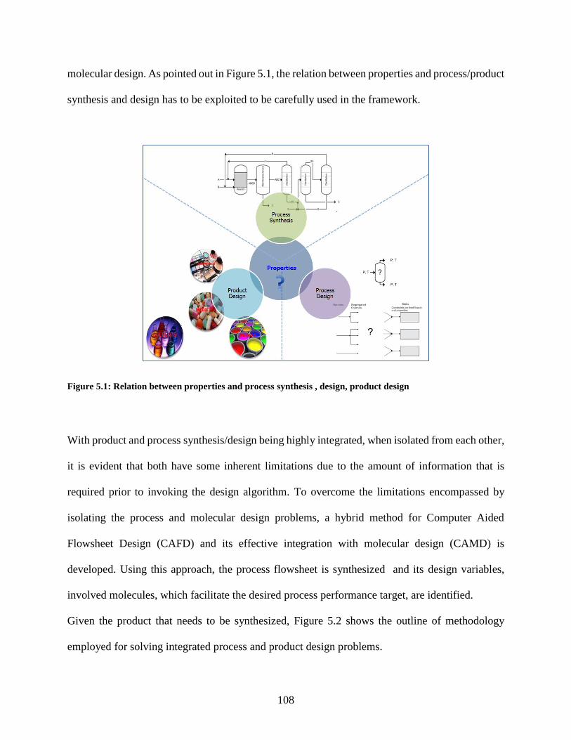
108
molecular design. As pointed out in Figure 5.1, the relation between properties and process/product
synthesis and design has to be exploited to be carefully used in the framework.
Figure 5.1: Relation between properties and process synthesis , design, product design
With product and process synthesis/design being highly integrated, when isolated from each other,
it is evident that both have some inherent limitations due to the amount of information that is
required prior to invoking the design algorithm. To overcome the limitations encompassed by
isolating the process and molecular design problems, a hybrid method for Computer Aided
Flowsheet Design (CAFD) and its effective integration with molecular design (CAMD) is
developed. Using this approach, the process flowsheet is synthesized and its design variables,
involved molecules, which facilitate the desired process performance target, are identified.
Given the product that needs to be synthesized, Figure 5.2 shows the outline of methodology
employed for solving integrated process and product design problems.

109
Figure 5.2: Methodology for integrated process and design.
Both the developed CAFD and CAMD frameworks are group contribution (GC) based approaches.
CAFD makes use of functional process groups, characterized by the type of unit operation/process
and their corresponding driving force, to generate and represent flowsheets; process group
contribution based property models to predict flowsheet properties from apriori regressed
contributions of process groups; a notation system for storing the flowsheet structural information;
and a synthesis method to generate and identify the feasible flowsheets. The identified candidate
flowsheets are ranked based on flowsheet properties (e.g. energy consumption, amount (mass) of
external agents used and/or cost/profit) representing flowsheet performance in a quantitative sense.
Once the promising flowsheet structures are identified, the flowsheet design parameters that
describe the process will be estimated. The reverse simulation method is used to calculate the
design variables of the unit operations involved in the process. This also gives a good estimate of
the important design parameters. Some alternatives may involve unit operations that require an
external agent. Also, the properties of any external agent needed by the process may depend on
potential existing recycle streams within the process. Thus, a property based platform is utilized

110
for integrating process and molecular design. The property clustering technique introduced by
Shelley and El-Halwagi (2000) provides the tools to track properties. Conventional agents may
not always meet the property constraints set by the reverse simulation design problem of such
operations. Novel agents can be identified by solving the product design problem, which includes
satisfying these property constraints. This is done by integrating the flowsheet design problem
with a molecular design problem. Depending on the type of unit operation in the process where an
external agent is required, the CAMD problem is formulated accordingly and the effect of the
solution alternatives from the CAMD problem on the process is evaluated by the process models.
CAMD includes building blocks (atoms and functional groups) to generate and represent
molecules; group contribution based property models to predict target properties; a standard
molecular structure notation system to store and visualize the molecular structure information; and
a synthesis method to generate and screen molecules that match the target (design) properties.
Once a set of near optimal flowsheet alternatives have been identified, rigorous simulation is used
to verify the predicted performance and select the best flowsheet. The framework also aims at
maintaining a good accuracy of solutions and large application range.
The principal concepts introduced in the chapter 2 are utilized to develop the framework shown
in Figure 5.2. The requirements for developing the framework are listed below:
Process Synthesis/Design
a) Systematic methods for selecting/screening unit operations involved in the process.
b) Simple string-like representations capable of systematically representing process
alternatives.
c) Models to calculate each flowsheet property.
d) Methods to synthesize flowsheets that meet the targets.

111
e) Method to calculate design parameters of the flowsheet.
Requirements a-c and e are based on available literature and listed in the next sections in the
sequence they are utilized. Requirement d is what is addressed in this dissertation and it is
one of the important step in CAFD.
Integration of Process & Molecular Design
a) Translation of information from process design problem to molecular design.
b) Nature of external agent based on the process recycle streams, type of unit operation
and solubility data.
These requirements are addressed in chapter 4.
Molecular Design
a) Models to calculate each desired molecular property.
b) Methods to synthesize molecules that meet target properties.
These requirements are addressed in chapter 3.
Hence, this chapter deals with developing an integrated framework for process and product
synthesis/design by using the concepts from literature and those shown in chapters 3 and 4.
5.2 Process Synthesis/Design by decomposition based approach
There are many different approaches to process synthesis including expert systems, optimization
or algorithmic methods, and conceptual methods based on physical insights. The objective here is,
given the raw materials and the desired product specifications, to develop a methodology that
systematically identifies the optimal process flowsheet transforming the raw materials into the
desired products in a more efficient manner. This dissertation highlights a novel hybrid method
for Computer Aided Flowsheet Design (CAFD) that combines physical insights with algorithmic

112
reverse design approaches to enable systematic identification of feasible flowsheets at significantly
reduced computational expense. Large number of components have to be dealt with while
developing a process flowsheet. Also, there are a wide range of unit operations that are available.
This leads to the possibility of a large number of process flowsheet alternatives. This complexity
is handled by a decomposition approach based on a targeted reverse methodology. Preliminary
screening of alternatives is done based on thermodynamic insights. Secondly, more promising
alternatives are screened based on performance indices. Finally the reduced list of alternatives are
verified using rigorous simulations. The developed framework utilizes the group contribution (GC)
approach developed by d’Anterroches and Gani (2005) in which, the flowsheets could be
represented using appropriate process descriptors. Also the framework relies on the exploited
relationships between properties and separation process principles by (Jaksland et al., 1995).
5.2.1 Methods for selecting/screening unit operations
For a typical process synthesis problem, the first thing to be known is if the required product is
naturally available (although in most cases with some impurities) or if a reaction route is needed
to synthesize it. Different reaction pathways based on the problem can be identified from literature.
Based on this background information different mixture streams can be imitated and the tasks of
identifying a) the respective upstream or downstream separation schemes b) the optimal among
all the identified process flowsheets remains to be worked on.
Separation of a mixture is caused by the addition of a separating agent, which takes the form of
another stream of matter or of energy (King, 1980). Separation processes in general can be
classified as three types – Mechanical separation processes, Equilibrium separation processes
(energy separating agent based and mass- separating agent based) and Rate – governed separation
processes. For any separation process classified as above, having an insight on their underlying

113
physical or chemical principles and phenomena, one or more specific pure component property
can be associated with it. Based on the evaluation of appropriateness of those characteristic
property differences between the key components of a mixture to effect the separations, respective
separation process may be selected as an alternative for separating/splitting the mixture across the
key components. One such physical insights based methodology is by (Jaksland et al., 1995). Here,
for a separation between two components and a given separation process, the separation process
can be checked for its feasibility based on the ratios of its corresponding pure component
properties. If the ratio is above a threshold value corresponding to this operation task and if some
additional property constraints are satisfied the operation task is considered as feasible. For
example, if the melting point ratio is larger or equal to 1.20 and the minimum value of melting
point is greater than a Tmin of 250K, crystallization is considered as very feasible separation
process for the binary mixture. The characteristic properties and their respective threshold limits
are given in the appendix. In some cases, where the very feasible separation processes cannot be
identified, just feasible separation processes can be considered as an alternative with a warning. In
identifying these, the trapezoidal representation (Qian & Lien, 1995) of threshold limits for a
separation process is applied. This representation helps in predicting the extent of feasibility of a
separation process for binary mixture.
5.2.2 Process Descriptors
The process groups by (d’Anterroches & Gani, 2005) are used in development of the framework.
The process flowsheet can be easily generated and represented by functional process-groups (PGs).
These PGs represent different unit operations such as reactor, distillation, extractive distillation
etc. and hence characterized by the type of unit operation. The bonds among the process groups

114
represent the streams connecting the unit operations. Also the separation PGs are characterized by
driving force and reactor PGs are characterized by their attainable region.
Driving Force
The driving force (DF) of component i with respect to component k in a binary pair for property
(or separation process) j, Dij, is given by
𝐷𝑖𝑗 = 𝑦𝑖 − 𝑥𝑖 =
𝑥𝑖𝛽𝑖𝑗
1 + 𝑥𝑖(𝛽𝑖𝑗 − 1) 5.1
Where, xi and yi are compositions of component i in two co-existing phases and βij is an adjustable
parameter with respect to separation process, j, that may be a constant or a function of other
variables (Gani & Bek-Pedersen, 2000). Also, it is evident that all the component indices are in
principle with respect to the second component k (in the binary pair). This difference in
composition of i in coexisting phases may be due to thermodynamic equilibrium in case of
equilibrium separation processes like distillation. Nevertheless, transport mechanisms other than
thermodynamic equilibrium, for instance diffusion or convection, can also promote driving forces,
and enable the separation to take place. For different compositions of i, we can hence obtain
corresponding DF by knowing 𝛽𝑖𝑗 for a given separation process or phase composition data.
Figure 5.3 gives the graphical representation of the phase composition data (that is, plot of the DF
as a function of liquid (or vapor) composition). It can be seen that DF in general is a concave
function with respect to composition with a well-defined maximum. Since, using the maximum
driving force for a given operation enables it to cause the change easily, the energy needed to be
added to or removed from the system to create and maintain two coexisting vapor liquid phases is
indirectly related to the DF. i.e. if DF is large, less energy is involved, while if DF is small more
energy is involved. Hence having this information readily available for a PG, we can have an
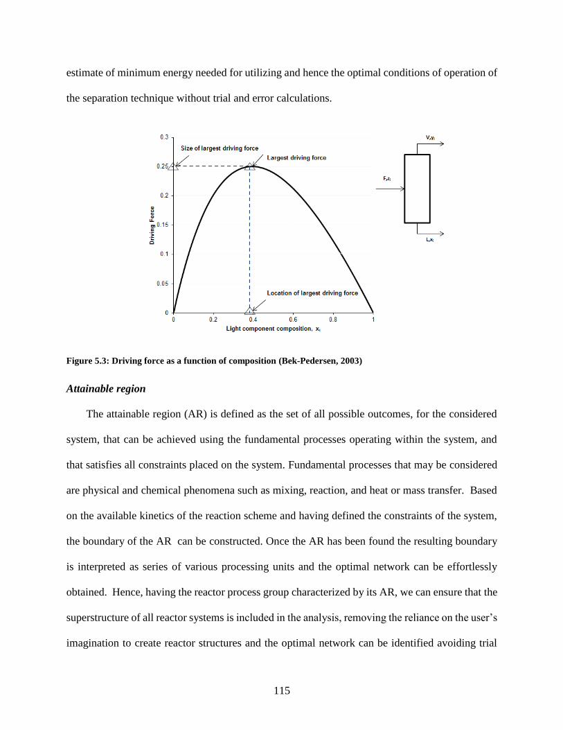
115
estimate of minimum energy needed for utilizing and hence the optimal conditions of operation of
the separation technique without trial and error calculations.
Figure 5.3: Driving force as a function of composition (Bek-Pedersen, 2003)
Attainable region
The attainable region (AR) is defined as the set of all possible outcomes, for the considered
system, that can be achieved using the fundamental processes operating within the system, and
that satisfies all constraints placed on the system. Fundamental processes that may be considered
are physical and chemical phenomena such as mixing, reaction, and heat or mass transfer. Based
on the available kinetics of the reaction scheme and having defined the constraints of the system,
the boundary of the AR can be constructed. Once the AR has been found the resulting boundary
is interpreted as series of various processing units and the optimal network can be effortlessly
obtained. Hence, having the reactor process group characterized by its AR, we can ensure that the
superstructure of all reactor systems is included in the analysis, removing the reliance on the user’s
imagination to create reactor structures and the optimal network can be identified avoiding trial

116
and error calculations. For example, for the trambouze reaction scheme, defined by the following
reaction set and kinetics, the AR in concentrations of A&C space is shown in Figure 5.4. It shows
that the boundary of AR is defined by a “bypassed” CSTR reactor between point O and A, followed
by plug flow reactor.
Reactions of trambouze reaction scheme:
𝐴 → 𝐵(1)
𝐴 → 𝐶(2)
𝐴 → 𝐷(3)
5.2
Reaction kinetics of trambouze reaction scheme:
𝑟1 =
𝑘1𝑐𝐴1 + 𝑘4𝑐𝐴
𝑟2 → 𝑘2𝑐𝐴(2)
𝑟3 =𝑘3𝑐
2𝐴
1 + 𝑘5𝑐2𝐴
5.3

117
Figure 5.4: Example of attainable region for the trambouze reaction scheme.
Again, it is also evident that since flowsheet synthesis is done based on the premise that each
separation process operates utilizing maximum driving force, the purity of outlet process groups
can be ensured to be at least 99.5% pure. This enables the simple mass balance around process
groups at the final stage.
Figure 5.5 shows a flowsheet with reaction process group, distillation, membrane separation
process group and a extractive distillation process group along. It can be seen that the process
groups represent either a unit operation (such as reactor, distillation, flash), or a set of unit
operations (such as, two distillation columns in extractive distillation, pressure swing distillation).
Consider the process flowsheet in Figure 5.5; the feed mixtures are represented by two inlet process
groups; (iA), (iB). The end products are represented by four outlet process groups; (oA), (oB), (oC),
(oD). The four process groups representing a reactor (rAB/pABCD), distillation (AB/CD), a solvent
based separation (cycB/C) and a molecular sieve separation (msA/B) have at least one inlet and one
outlet streams.

118
It is evident that, the same process groups can be used to represent different components having
similar properties. Note, however, that the inlet and outlet streams (bonds) of process groups must
maintain the list of components present in them and that the path of a component through a process
group establishes the flowsheet structure. That is, process groups (AB/CD) and (msA/B) can be
connected to form [(AB/CD)(msA/B)] without knowing the identities of the components A, B, and
C. Only when the properties of the flowsheet need to be calculated, the identities of the chemicals
(components) are needed.

119
Figure 5.5: Representation of flowsheet (a). with process groups (b, c) process groups

120
Currently, seventeen process groups are available (Alvarado, 2010). These are listed in Table 5.1.
Table 5.1: Available Process groups (Alvarado, 2010).
Unit Operation Process-group example
Simple Distillation Column (AB/C)
Solvent Based Azeotropic Separation (cycA/B)
Flash Separation (fAB/CD)
Kinetic Model Based Reactor (rABC/nE/pABCD)
Fixed Conversion Reactor (rABC/nE/pABCD)
Pressure Swing Distillation (swA/B)
Polar Molecular Sieve Based Separation (pmsABC/D)
Molecular Sieve Based Separation (msABC/D)
Liquid Membrane Based Separation (lmemABC/D)
Liquid Adsorption Based Separation (ladsABC/D)
Gas Membrane Based Separation (gmemABC/D)
Pervaporation Based Separation (pervABC/D)
Crystallization Based Separation (crsABC/D)
Liquid Liquid Extraction Based Separation (lleABC/S/SC/AB)
Simple Solid Liquid Separation (slAB/CD)
Absorption (abEAB/eF/EABF/EF)
Ion Exchange Separation (ieABCD/ABC)

121
This kind of representation of the involved streams and unit operations in a process also gives an
additional benefit of being able to represent the flowsheets by a simple line entry called SFILES
(Simplified Flowsheet Input Line Entry System) (d'Anterroches, 2006). This enables easy
representation of the synthesized flowsheets.
Simplified Flowsheet Input Line Entry System
According to d'Anterroches (2006), any flowsheet comprising of the above described PGs can be
represented by a unique SFILES. This concept in turn can be traced back for its roots to SMILES
(Simplified Molecular Input Line Entry System) (Weininger, 1988). If in a flowsheet, the analogy
between flowsheet and a graph; its PGs and graph nodes; connection between PGs and graph edges
respectively is established, a unique representation of each flowsheet by a SFILES representation
is maintained by canonicalization of a graph using the product of corresponding primes function
on the ranks of each node based on the ranks of their invariant set. In Figure 5.6, flowsheets with
and without recycle streams are shown to be represented by their respective SFILES. Branches in
the flowsheet are represented within square brackets and recycle stream are represented by
numbers. Also, owing to the fact that PGs can be connected in only one direction, the orientation
of the group when not following left to right direction is clarified by a smaller than symbol (<).

122
Figure 5.6: SFILES notation of a simple flowsheet (a) without recycle (b) with recycle.
Determining unique SFILES for a flowsheet prevents ambiguity and provides its own share of
computational benefits during flowsheet synthesis. For example, when a number of flowsheet
alternatives are generated for a problem, checking if an alternative is already found becomes easy
with this SFILES representation. Also, by virtue of how these are made to describe a flowsheet
uniquely, they can help in efficient transfer/storage of PG information for a flowsheet.
Finally having the flowsheets described by well characterized PGs and represented by SFILES,
the property of a flowsheet can be easily identified using a GC based property model. This surfaces
from the fact that this representation of flowsheets by PGs is part of utilizing GC techniques to
flowsheet synthesis. d’Anterroches and Gani (2005) pointed out that energy consumption of a
process flowsheet is one flowsheet property which can be predicted by a GC based property model.

123
Hence, the separation PGs along with being characterized by type of unit process/operation and
driving force should be also characterized by their contributions towards the flowsheet property of
interest.
Flowsheet property model
d'Anterroches (2006) shows that a flowsheet property – energy consumption of a flowsheet can be
represented by a sum of process group contributions towards this property.
𝑓(𝑃) = 𝐸𝑥 =∑𝑝𝑜𝑠𝑘 ∙ 𝑎𝑘
𝑁𝐺
𝑘=1
5.4
where, 𝐸𝑥 is the flowsheet property – energy consumption; NG is the number of process groups;
𝑎𝑘 is the regressed contribution of PG, k and 𝑝𝑜𝑠𝑘 is the topology factor.
As stated above, it is clear that any PG is component independent if it is based on the driving force.
Hence, a general property model irrespective of its components can be derived. The contributions
𝑎𝑘 of the process groups can be regressed by means of fitting experimental data.
5.3 The CAFD framework integrated with CAMD framework.
In any GC based method, as long as the structure can be fully described with the groups, the
properties of the structure are immediately available. So, these methods can be used to synthesize
new structures easily as the evaluation of the properties of a structure is straightforward given the
models and the group contributions. In CAFD, based on a GC method, flowsheets are described
by process groups and the goal of generating flowsheet structures matching the target properties
within the structural constraints is achieved easily without the need of rigorous models. Also from
the information the process groups carry, the minimum set of design parameters to fully describe
the flowsheet can be identified.

124
The CAFD framework, based on the GC-concept is handled by the following steps: a) Problem
Definition and Analysis (analyze the synthesis/design problem to define the performance criteria
in terms of a set of target properties and to establish the desired target property values; define the
initial search space in terms of a superstructure of alternatives); b) Process Synthesis (generate and
screen process flowsheet alternatives); c) Process Design (determine the equipment/operation
designs for the selected feasible process flowsheets); and d) Process Verification (verify the design
through rigorous simulation and/or experiments). The outline of the CAFD framework and
necessary information at each stage is shown in Figure 5.7.
Figure 5.7: CAFD framework.

125
5.3.1 Problem Definition & Analysis
Given the raw materials and the desired product specifications, the problem is to identify the
optimal process flowsheet that transforms the raw materials into the desired products in the most
efficient manner. The problem is later analyzed to define the type of process that needs to be
synthesized, e.g. processes with or without reaction based on the raw materials and product
specifications; to identify the phases (vapor, liquid, and/or solids) that may be involved; to
determine the number of operations/tasks that need to be performed; to select the types of unit
process/operations that may be involved in the flowsheet alternatives based on rules proposed by
Jaksland et al. (1995); to select the performance criteria by which to evaluate the process flowsheet
alternatives.
Figure 5.8: Problem analysis steps (Jaksland et al., 1995).
Reaction Analysis
If in the definition of the problem, desired product components are different from raw materials,
it is clearly evident that chemical conversion of raw materials to products is needed. In such cases,
a database search can be performed to identify the reaction routes making the chemical
transformation possible. Depending on the knowledge of reaction rates or conversion rates of the

126
involved reaction routes, we can initialize the kinetic reactor or fixed conversion reactor PGs,
respectively along with the inlet PGs for raw materials. If more than one reaction are involved and
have to occur sequentially in the selected route, corresponding reaction PGs are initialized for each
of them which may have to be connected by separation PGs or recycle streams. Another interesting
evaluation would be to check for the possibility of simultaneous reaction+separation processes.
This kind of evaluation about the possibility of simultaneous reaction+separation process can be
made by having an insight of the nature of side reactions, involved inerts, as well as Damkohler
numbers (Kulprathipanja, 2001) and is beyond the scope of this dissertation. But once the
possibility of such groups is established, the reaction+separation PGs can be easily used within the
scope of the developed framework. Finally with the reaction process groups in hand, resulting
mixtures from each of them can be initialized and the separation schemes for the mixtures
depending on the problem definition have to be synthesized.
Pure Component and Mixture Analysis
The nature of each of the mixtures obtained is determined at this stage. This kind of
preliminary assessment enables the selection or rejection of separation operations. If for example,
two of the components in the mixture tend to form azeotropes, distillation operation may be ruled
out for that pair. Here preliminarily, the following information about the mixture is identified at
the given reference conditions.
a. State of components (vapor, liquid, and/or solids).
b. Pure component properties.
c. Bulk/dilute components (if compositions of components are known).
d. Polar/non polar components.
e. Azeotropes [hetero/homo] and eutectic points.

127
f. Temperature sensitive components.
g. Toxic components.
Also, all possible preliminarily information is gathered at this stage. This information helps
in deciding on the thermodynamic models for predicting phase equilibrium when necessary.
The 22 pure component properties listed in Table 5.2 are identified using available chemical
databases or using any property prediction models.
Table 5.2: List of considered pure component properties
Property Secondary/Primary
MW Molecular Weight (g/mol) Primary
ω Acentric Factor Primary
Tc Critical Temperature (K) Primary
Pc Critical Pressure (bar) Primary
Zc Critical Compressibility Factor Primary
Vc Critical Volume (m3/kmol) Primary
Tb Normal Boiling Point (K) Secondary
dm Dipole Moment ×1 · 10−30 (C · m) Primary
rg Radius of Gyration (nm) Primary
Tm Melting Point (K) Secondary
Ttp Triple Point Temperature (K) Primary
Ptp Triple Point Pressure (Pa) Primary
Mv Molar Volume (m3/kmol) Secondary
Hf Ideal Gas Heat of Formation (kJ/kmol) Secondary

128
Gf Ideal Gas Gibbs Energy of Formation (kJ/kmol) Secondary
SI G Ideal Gas Absolute Entropy (kJ/(kmol · K)) Secondary
Hfus Heat of Fusion at Tm (kJ/kmol) Secondary
Hcomb Standard Net Heat of Combustion (MJ/kmol) Secondary
δ Solubility parameter (kJ/m3) Secondary
Vvw Van der Waals Volume (m3/kmol) Primary
Avw Van der Waals Area (m2/kmol) Primary
Pnvap Normal Vapor Pressure (Pa) Secondary
Having this data in hand, mixture analysis can be made by enumerating all possible binary pairs
and calculating their respective ratio of all above 22 properties.
If NC is the number of components in the mixture, the number of binary pairs,
𝑛𝑏𝑖𝑛 is given by:
𝑛𝑏𝑖𝑛 =
𝑁𝐶(𝑁𝐶 − 1)
2 5.5
And the number of separation tasks, 𝑛𝑠𝑒𝑝 if sharp split between components is aimed at is given
by:
𝑛𝑠𝑒𝑝 = 𝑁𝐶 − 1 5.6
This enables the identification of feasible separation techniques/operations for each binary
separation task.
For all 𝑖 = 1𝑡𝑜𝑛𝑏𝑖𝑛 binary pairs, the property ratio, 𝑟𝑖𝑗𝑘 corresponding to jth property and kth
separation technique is given by

129
𝑟𝑖𝑗 =
𝑃𝑗,𝐴
𝑃𝑗,𝐵 ; 𝑃𝑗,𝐴 ≥ 𝑃𝑗,𝐵 5.7
For the properties marked as secondary in Table 5.2, the binary values may be calculated over a
range of pressure or/and temperature. Doing this gives the initial estimates of conditions of
operation of a separation technique.
Selection of Candidate Separation operations
The rules proposed by Jaksland et al. (1995) as explained in section 5.2.1. are utilized here. With
the limits on the property ratios for a separation operations/techniques to be used for a binary
separation task set a-priori from literature, by comparing the above tabulated binary property ratios
against these limits, candidate separation tasks can be identified. The limits on property ratios for
different separation operations are given in Appendix B.
This can be mathematically explained as follows:
For a binary pair i = 1 to 𝑛𝑏𝑖𝑛 and separation operation/technique, k and and property j, the upper
and lower limits of corresponding separation technique’s property, 𝑟𝑖𝑗𝑘 are given by a trapezoidal
form of limits (Qian & Lien, 1995) as below:
𝐿𝑜𝑤𝑒𝑟𝑙𝑖𝑚𝑖𝑡𝑠 ∶ [𝑚𝑘,𝑗 , 𝑀𝑘,𝑗]
𝑈𝑝𝑝𝑒𝑟𝑙𝑖𝑚𝑖𝑡𝑠 ∶ [𝑁𝑘,𝑗, 𝑛𝑘,𝑗] 5.8
The feasibility of a separation technique is then decided by:
𝑟𝑖𝑗𝑘 ≤ 𝑚𝑘,𝑗 − −→ 𝜇(𝑟𝑖𝑗𝑘) = 0&𝑘𝑖𝑠𝑖𝑛𝑓𝑒𝑎𝑠𝑖𝑏𝑙𝑒𝑓𝑜𝑟𝑖
𝑚𝑘,𝑗 ≤ 𝑟𝑖𝑗𝑘 ≤ 𝑀𝑘,𝑗 − −→ 𝜇(𝑟𝑖𝑗𝑘) =(𝑟𝑖𝑗𝑘 −𝑚𝑘,𝑗)
(𝑀𝑘,𝑗 −𝑚𝑘,𝑗)&𝑘𝑖𝑠𝑓𝑒𝑎𝑠𝑖𝑏𝑙𝑒𝑓𝑜𝑟𝑖
𝑀𝑘,𝑗 ≤ 𝑟𝑖𝑗𝑘 ≤ 𝑁𝑘,𝑗 − −→ 𝜇(𝑟𝑖𝑗𝑘) = 1&𝑘𝑖𝑠𝑣𝑒𝑟𝑦𝑓𝑒𝑎𝑠𝑖𝑏𝑙𝑒𝑓𝑜𝑟𝑖
5.9

130
𝑁𝑘,𝑗 ≤ 𝑟𝑖𝑗𝑘 ≤ 𝑛𝑘,𝑗 − −→ 𝜇(𝑟𝑖𝑗𝑘) =(𝑛𝑘,𝑗 − 𝑟𝑖𝑗𝑘)
(𝑛𝑘,𝑗 − 𝑁𝑘,𝑗)&𝑘𝑖𝑠𝑖𝑛𝑓𝑒𝑎𝑠𝑖𝑏𝑙𝑒𝑓𝑜𝑟𝑖
𝑟𝑖𝑗𝑘 ≥ 𝑛𝑘,𝑗 − −→ 𝜇(𝑟𝑖𝑗𝑘) = 0𝑎𝑛𝑑𝑘𝑖𝑠𝑖𝑛𝑓𝑒𝑎𝑠𝑖𝑏𝑙𝑒𝑓𝑜𝑟𝑖
Additionally
0 ≤ 𝜇(𝑟𝑖𝑗𝑘) ≤ 1 − −→ 𝐴𝑤𝑎𝑟𝑛𝑖𝑛𝑔𝑜𝑛𝑘𝑓𝑜𝑟𝑖𝑖𝑠𝑖𝑠𝑠𝑢𝑒𝑑 5.10
Finally, separation techniques which might be feasible at extreme T, P ranges are considered as
infeasible at the preliminary stage. Only when no flowsheet can be synthesized, these separation
techniques are reconsidered.
5.3.2 Flowsheet Synthesis
Once the problem has been analyzed, the objective here is to generate and evaluate feasible
flowsheet alternatives based on the selected process groups; the minimum number of processing
steps and the product specifications. A number of methods and tools are needed here. Flowsheet
synthesis was earlier done by d’Anterroches and Gani (2005) and Alvarado (2010) but owing to
the high combinatorial nature of the problem, a systematic method for processing of data from
problem analysis is needed. In earlier works, all the possible PGs are initialized irrespective of
constraints related to connections and are then connected. In such cases, the list would be large
and may contain many useless PGs leading to structurally infeasible flowsheets. This tedious task
can be avoided by a much more sophisticated way of generating the flowsheets as explained below.
Hence, initialization and connecting the PGs is done hand in hand in this work.
Owing to the PG’s characteristics, the PGs by themselves are property dependent and component
independent while connections between the PGs are component dependent. As PGs are component
independent, for any PG of a particular separation technique type, one for each set of components

131
can be initialized provided its characteristic property ratio between key components falls into
feasible limits of the separation technique.
Generation of Superstructure with Initialized Process Groups
Initialization of Process Groups
Here, instead of initializing all PGs for different separation techniques at once, for each product
mixture when encountered, the separation PGs of different separation technique type are initialized
with respect to the number of chemicals and their identities. This is done through the following
three step procedure and each step is illustrated through an imaginary mixture list.
1. Order mixture components wrt. characteristic property for each feasible separation task.
For example:
Table 5.3: Illustration of component order table.
2. Order feasible binary splits based on property ratio (ease of separation)

132
Table 5.4 : Illustration of binary split order table.
3. Initialize the PGs involving all components of the mixture: For each separation technique,
only the PGs with the highest property ratios are initialized. This constraint reduces the
number of initialized PGs that could form practically feasible flowsheets. If the binary pair
with the highest property ratio for any of the separation technique in not of adjacent
components from the component order table, the PGs with next highest property ratio are
initialized. From Table 5.4, the S1A/C PG falls into such category.
Table 5.5: Initialized PGs of a ABC mixture.
Again, if separation barriers affect the separation task further analysis is done to keep the
PG in and also the effect of non-key components on the properties enabling separation are
checked before initializing the process group. For example, If S3 is a distillation based PG,
and AC forms an azeotropic mixture and only sharp splits are considered, S3(CB/A) is
eliminated from the set of initialized PGs as azeotropic AC becomes a separation barrier

133
to S3. If azeotropes or eutectic mixtures exist in the component, they have to be considered
as a single entity and ordered accordingly in the component order table before initializing
any PG involving them.
The algorithm for initializing PGs for a mixture is shown in Figure 5.9.
Figure 5.9: Initialization of PGs for an mixture encountered in runtime.

134
Generation of Superstructure
The superstructure for each of the initial mixtures (defined by the problem or from initialized
reaction PGs) is generated using the following methodology. Once the PGs for each of these
mixtures are initialized, the consequent mixture lists resulting from these PGs are listed and if they
comprise of more than one component, their matching PGs are initialized using the algorithm in
Figure 5.9 else an outlet PG is initialized. This is continued until no mixture is left. As each PG
carries the information of the number and identity of the components along with the separation
task, this information can be utilized to impose structural constraints on the consequent PGs by
limiting the number of PGs that could be linked to the parent PG in the super structure. Hence,
here basically, the tree lists of PGs resulting from its parent PGs are made. Figure 5.10 gives an
example of one such superstructure involving imaginary component lists and unit
operations/processes.
Figure 5.10: Illustration of PGs superstructure.

135
If for all the components from the initial mixture (A,B,C), outlet PGs exist in the
superstructure, the header PG can be termed as a feasible first order group and the
superstructure remains in the list for further processing else it can be discarded or the problem
can be reanalyzed relieving some constraints on separation techniques. The algorithm for
generating a superstructure is shown in Figure 5.11.
Figure 5.11: Generation of superstructure of PGs.

136
As each PG carries the information of the number and identity of the components along with the
separation task, this information is utilized to impose structural constraints on the consequent PGs.
Finally from the list of superstructures combinations, flowsheets leading to targeted product
components are identified and represented by their unique SFILES.
SFILES Representation of Flowsheets
All feasible flowsheets generated in this step are represented by their corresponding SFILES
notation according to the method developed by d'Anterroches (2006) and stored in terms of this
notation. In order to generate the feasible SFILES, all paths from the generated superstructures are
populated and combined to form a binary tree structure such that the combination has NC
components (the number of components in the initial mixture/product of the initial reactor PG of
a superstructure), sharp splits and NC-1 separation PGs involved. Once these trees are formed,
each PG is denoted with an invariant as described in d'Anterroches (2006). The root node is first
selected each time and branching decisions are taken based on the invariant of PG, the one with
lowest is selected first. The rules to denote a PG with an invariant is shown in appendix. Figure
5.12 gives an example of a tree representation and its SFILES representation. The algorithm to
generate SFILES is given by Figure 5.13.

137
Figure 5.12: (a) Tree representation of a combination, (b) SFILES representation of the feasible flowsheet
Figure 5.13: Algorithm for SFILES generation.

138
Ranking of Flowsheet Alternatives
The target properties for each generated feasible flowsheet alternative are calculated using the
flowsheet property models combined with a-priori calculated property contributions of each PG.
The target property models may be only structure dependent (primary properties), or, they may be
dependent on multiple phenomena (effect of energy and mass separating agents). Based on these
target properties, the flowsheet alternatives that are structurally feasible and that satisfy the
property targets are identified. Currently, there are property models to assess the performance in
terms of energy consumption for distillation, flash, solvent based distillation process groups and
pressure swing distillation PGs. The flowsheet property model is given by:
𝐸 = ∑1+ 𝑝𝑘
𝑑𝑖𝑗𝑘
𝑁𝐺
𝑘=1
×𝑎𝑘 5.11
where, E is the energy consumption performance of the flowsheet, NG is the number of PGs, 𝑑𝑖𝑗𝑘 is
the maximum driving force of PG, k, 𝑎𝑘 is the contribution of PG, k and 𝑝𝑘 is the topology factor
given by
𝑝𝑘 =∑𝐷�̅�
𝑛𝑡
𝑖=1
5.12
where, nt is the number of separation tasks that should be performed before the task, k and 𝐷�̅� is
the maximum driving force of task, i. The PG contribution are taken from Alvarado (2010);
d'Anterroches (2006) and are listed in appendix.
5.3.3 Process Design and integration with Molecular Design
The objective here is to determine the optimal values of the minimum number of design variables
corresponding to each process equipment and/or operation in the selected feasible flowsheet. For

139
counter-current staged separation processes, this includes variables such as number of stages, feed
location, product specifications and reflux ratio. For reactors, examples of the design variables are
reactor volume, residence time, reactor effluent composition, and temperature. With the reverse
approach, separation related PGs such as distillation, extractive distillation, and flash drums are
characterized in terms of their driving force (Bek-Pedersen, 2003) while reaction related PGs are
characterized in terms of their highest attainable reaction point (Horn, 1964). The design method
back-calculates the design variables from the highest driving force or highest attainable reaction
point. The detailed methodology for each of this can be understood through methodologies shown
in appendix as well as part of the case studies.
Some of the unit operations may be in need of an external agent and as stated, the performance of
the flowsheet varies depending on the external agent. Process and product design are closely
related and failing to correctly achieve the simultaneous design can lead to unexpected results like
increase in cost of production etc. Having process models that can rapidly evaluate the impact on
a process of a change of an involved component, based on the process type a CAMD problem is
set up to identify the feasible external agent corresponding to the molecular design targets
translated from the targets set by the process design problem. Also as the PGs carry all information
about the properties of its inlet and outlet components, the process design methodology given in
section 4.3 can be utilized to identify property targets on the external agent (like a solvent)
depending on the other streams in the process. Finally, the best option among the solutions to
CAMD problem can be chosen based on its effect on the process.
CAMD
To design the external agents, the CAMD methodology developed by Bommareddy et al. (2010a)
is used. Depending on the type of unit operation the process targets are translated into targets for

140
the CAMD problem. In the developed CAMD methodology which is given in chapter 3, the
molecular structures that match the targets are identified by a reverse property prediction problem.
The molecules designed are further screened based on the mixture property targets. With each
feasible molecule found, different flowsheets with corresponding properties are identified and
ranked.
5.3.4 Final Verification
The objective here is to verify the synthesis/design results from the previous steps as well as to
determining the remaining unknown variables of the process. This is done through rigorous
simulation using design variables identified by reverse simulation provided the necessary models
are available. As the design corresponds to maximum driving force and/or highest attainable
region, the candidate design should correspond to the minimum energy requirement design. If
necessary, the design can be verified experimentally with the established optimal operating
conditions and equipment parameters.
5.3.5 Software Implementation
The CAFD and CAMD methods involve screening a lot of data and it is practically impossible to
apply them without an efficient software implementation. A beta version of the tool for the CAFD
has been developed based on the framework using VC++ - Microsoft Foundation Class Libraries.
The data flow of the CAFD framework along with the solution steps is given by Figure 5.14.

141
Figure 5.14: Data flow in the CAFD framework.
The beta version of the tool considers the problem analysis being done and given the unit
operations that could perform the binary separation tasks, the tools works to initialize the PGs and
generate the list of SFILES with their respective property. Once the tool generates the list the
optimal flowsheet could be selected, designed and verified. The steps as seen by the user of the
tool are shown in the Figure 5.15.

142
Figure 5.15: View of the developed CAFD tool
5.4 Summary
This chapter presented a novel systematic framework for CAFD integrated with CAMD. The
CAFD methodology is based on GC concepts, and when integrated using the reverse problem
formulation technique with CAMD leads to very efficient simultaneous process and product
synthesis/design, while keeping the high level of accuracy associated with the group contribution
methods. The architecture of the developed prototype software has been presented and its
utilization is shown by developing the following interesting application examples.

143
5.5 Case Studies – Computer Aided Flowsheet Design
5.5.1 Case Study – Production of Isobutene
Problem statement
Isobutene is a potential starting material for production of butyl rubber, poly isobutylene etc. In
this case study, the production of isobutene by decomposition of Methyl tert Butyl Ether at about
493K is investigated. The objective is to identify the optimal process configuration by minimizing
the energy requirements. The potential reaction pathways to form Isobutene are identified as
shown in Equations 5.13, 5.14 and 5.15.
MethyltertButylEther®Methanol + Isobutene 5.13
Methanol®DimethylEther + Water 5.14
Isobutene®IsobuteneDimer 5.15
For the sake of initializing PGs and easy representation of components in a mixture, the
components involved in the above reactions are denoted by
A Methyl tert Butyl Ether
B Methanol
C Isobutene
D Dimethyl Ether
E Water
F Isobutene Dimer

144
Since the conversion is incomplete, the product (Isobutene) needs to be recovered and then purified
from the reactor effluent while the reactants recycled to the reactor. The reactor affluent stream
consists of all A-F components. Each of the components is to be recovered at > 99% purity.
Problem Analysis
Since the reaction route is given, the reactor PG - (rA/pABCDEF) is initialized. The total number
of components in the resulting mixture from reaction is six. Hence minimum number of separation
processing steps is five. Pure component properties and mixture properties are analyzed at
reference conditions of 298K and 1 atm. The mixture properties are in terms of the ratios of
properties of all the possible fifteen binary pairs among the components in the mixture. The initial
mixture analysis identifies the azeotropes among the components listed in Table 5.6.
Table 5.6: Azeotropes at 1 atm pressure.
Azeotrope T(K) & x(mole %) Azeotrope type
B/C 266.2K – 0.2% B Min Boiling
B/F 336K – 86.9% B Min Boiling
F/E 346.1K – 67.3% E Min Boiling
A/E 325.6K – 96.5% A Min Boiling
B/A 325.54K – 68.2% A Pressure sensitive
The feasible separation techniques identified using rules from Jaksland (1996) are shown in Table
5.7.

145
Table 5.7: Separation tasks and potential techniques for Isobutene production.
Flowsheet Synthesis
At this stage the developed software is initiated with all the information and all the SFILES with
their respective flowsheet properties (based on only distillation columns at this stage) are obtained.
Separation Technique Property Ratio Threshold Values Separation Tasks
Azeotropic Distillation Azeotrope B/F, B/A, F/E, A/E
Liquid-Liquid Extraction Azeotrope B/F, B/A, F/E, A/E
Molecular Sieve
Kinetic Diameter > 1.05
van der Walls Volume > 1.07
Polarisability > 1.0
Dipolemoment>1.05
B/F, B/D, B/C, B/A, F/D,
D/C, D/E
Pressure Swing
Distillation
Pressure sensitive azeotrope B/A
Distillation
Boiling point > 1.01
Vapor Pressure>1.05
B/D, B/E, F/D, F/C, F/A,
D/A, D/E,C/E
Flash
Boiling point > 1.23
Vapor Pressure>10
B/D, F/D, F/C, D/A, D/E,
C/E

146
Figure 5.16: Generation of SFILES using the CAFD tool.
This information hence was provided to the developed CAFD tool and 12 feasible flowsheets were
identified as shown in Figure 5.17 from the candidate process groups represented by the
corresponding SFILES notation.
Figure 5.17: SFILES identified by the CAFD tool for Isobutene production problem.

147
The energy index flowsheet property was calculated for all candidate configurations and the
SFILES string with the energy index (0.1575) is selected for design. It is combined with the inlet
PGs and reaction PGs. The obtained configuration consists of a reactor and five separation units:
molecular sieve, extraction and three distillation columns.
(rA/pABCDEF)(lleEBFDAC/S/SEB/FDAC)[(B/SE)(oSE)[(oB)]][(DC/AF)[(A/F)[(oF)]
(oA)](msC/D)[(oD)](oC)
Figure 5.18: Selected optimal flowsheet.
Before invoking the molecular design problem to identify the solvent for LLE PG, it is evident
that methanol is highly soluble in water (one of the components in the mixture) while other

148
components in the mixture are not soluble in water. Hence, this information confirms water as the
candidate solvent for the extraction unit. But in many cases it’s not simple to find a solvent like
water, hence a thorough emphasis has to be put on setting the targets for the molecular design
problem and the solvents may be found using any CAMD tool (like the one by Bommareddy et al.
(2010a).
The contributions towards the flowsheet property model are currently available for only distillation
process groups. The flowsheets generated using the software have different number of distillation
type PGs and hence the flowsheet having less number of distillation PGs in them might have the
least property value. The contribution of PGs other than distillation type may be high or low.
Therefore in the current case study an old heuristic: “prefer distillation columns first” is used to
select the flowsheet shown in Figure 5.18. Once the contributions from PGs of other than
distillation type are found as cited in the future work shown in this dissertation, the optimal
flowsheet could be selected without the help of heuristics. Also this case study can be compared
with the flowsheet for separation of the mixture from isobutylene production (Yamase & Suzuki,
2005) – as shown in Figure 5.19. Sharp splits have been considered at each stage. The unit
operations used and their order looks to be similar to the published one.

149
Figure 5.19: Flowsheet from literature (Yamase & Suzuki, 2005).
Flowsheet Design
The LLE PG does not involve energy consumption; the maximum solvent free driving force is
used as the performance criterion. Knowing the solvent free driving force of the unit, the amount
of solvent can be estimated. The higher the maximum driving force, the less solvent is required.
Here for this process group the LLE data between water, methanol, and Isobutene dimer are to be
available for further calculations. This information could not be readily retrieved from literature.
If more than two solvents are feasible, their respective maximum driving force corresponding to
given solvent amount or solvent amount corresponding to selected driving force can be used in a
comparative sense. The solvent with larger maximum driving force value or the one that when
used in lesser quantity does the job is the optimal solvent. The reverse simulation of the distillation

150
columns using the driving force approach (Gani & Bek-Pedersen, 2000) yielded a design operating
at the maximum driving force. The design parameters are shown in Table 5.8. The VLE data for
the key components in each distillation column is taken from literature and the maximum driving
force (difference between vapor phase composition and liquid phase composition) is noted.
Table 5.8: Design parameters of distillation columns
These conditions can be used as initial conditions for performing the rigorous simulation to
validate the obtained optimal flowsheet further.
5.5.2 Case Study – Production of Diethyl Succinate
Succinic acid is a potential co-product from bioethanol manufacture, which can be further reacted
with ethanol to produce diethyl succinate (DES), a useful solvent for cleaning metal surfaces and
paint stripping. In this case study, the production of diethyl succinate from ethanol and succinic
acid is investigated. The objective is to identify the optimal process configuration by minimizing
Parameter (DC/AF) (E/B) (A/F)
Max driving force (from VLE data): 0.5078 0.3916 0.4919
Light key composition at max driving force,
Dx ( from VLE data):
0.22 0.2 0.2
Recovery of light key (from definition of PG): >0.995 >0.995 >0.995
Ideal no. of stages (from (Gani & Bek-
Pedersen, 2000) or knowledge) :
20 15 20
Feed location (= Ideal No of stages *(1- Dx) ): 15 12 16
Min Reflux Ratio (from (Gani & Bek-
Pedersen, 2000)) :
0.4105 1.095 0.515

151
the energy requirements. The potential reaction pathways to form diethyl succinate are identified
as shown in Equations 5.16 and 5.17
SuccinicAcid + Ethanol®MonoethylSuccinate + Water 5.16
MonoethylSuccinate + Ethanol®DiethylSuccinate + Water 5.17
For the sake of initializing PGs and easy representation of components in a mixture, the
components involved in the above reactions are denoted by
A Ethanol
B Water
C Diethyl Succinate
D Monoethyl Succinate
E Succinic Acid
Since the conversion of succinic acid and ethanol is incomplete, the product (diethyl succinate)
needs to be recovered and then purified from the reactor effluent while the reactants recycled to
the reactor. Each of components is to be recovered at > 99% purity.
Problem Analysis
Since the reaction route is given, the reactor PG - (rAE/pABCDE) is initialized. From literature
Kolah, Asthana, Vu, Lira, and Miller (2008), a pervaporation assisted reactor is also considered as
one of the options for this system. Hence the reaction+separation PG – (rpervAE/pB/ACDE) is
also initialized. The total number of components in the resulting mixtures from the reaction PGs
are 5 and 4, respectively. Hence the minimum number of separation processing steps is four and
three, respectively. Pure component properties and mixture properties are analyzed at reference
conditions of 298K and 1 atm. The mixture properties are in terms of the ratios of properties of all
the possible ten binary pairs among the components in the mixture.

152
The initial problem analysis identifies the feasible separation techniques shown in Table 5.9.
Table 5.9: Separation tasks and potential techniques for DES production
The initialized PGs while generating the flowsheets is listed in Table 5.10.
Flowsheet Synthesis
Table 5.10: Initialized process groups for DES production.
Unit Operation Process Group
Reactor rAE/pABCDE, rpervAE/pB/ACDE
Crystallization crsE/DBCA, crsE/DCA, crsDBC/A, crsE/DC,
crsDC/A
Separation Technique Property Ratio Threshold Values Separation Tasks
Crystallization Melting Point > 1.27 A/C, C/E, D/E
Liquid Membrane
Radius of Gyration > 1.03
Molar Volume > 1.08
Solubility Parameter > 1.28
A/B, A/D, A/E, B/C, B/D,
C/D, C/E, D/E
Pervaporation
Molar Volume > 1.08
A/B, A/D, A/E, B/C, B/D,
C/D, C/E, D/E
Distillation
Boiling point > 1.01
Vapor Pressure>1.05
A/C, B/C
Flash
Boiling point > 1.23
Vapor Pressure>10
A/C, B/C

153
Liquid Membrane lmemCDEA/B, lmemCDE/A, lmemCDA/B,
lmemCD/E, lmemCD/A, lmemCD/B, lmemC/D,
lmemA/B
Pervaporation pervCDEA/B, pervCDE/A, pervCDA/B, pervCD/E,
pervCD/A, pervCD/B, pervC/D, pervA/B
Distillation AB/CDE, AB/CD, A/CDE, A/CD, B/CD
Flash fAB/CDE, fAB/CD, fA/CDE,fA/CD, fB/CD
The mixture analysis also reveals the existence of two binary azeotropes (water/diethyl succinate
and water/ethanol). Therefore, azeotropic distillation, extractive distillation, and liquid-liquid
extraction might also be potential separation techniques to be considered in the synthesis problem.
However, pervaporation and the liquid membrane selectively remove water from the mixture thus
alleviating the need for azeotropic separation. To enable the user taking such decisions the
developed tool interacts with the user to select the separation techniques for the tasks. A
pervaporation assisted reactor is found to be an efficient configuration for esterification reactions.
The PGs highlighted in blue in Table 5.10 are the potential first separation operations for the
reactor mixture, ABCDE. Similarly they could be identified for mixture ACDE. A total of 176
feasible flowsheets were identified from the candidate process groups and represented by the
corresponding SFILES notation. The energy index flowsheet property was calculated for all
candidate configurations and the two SFILES strings with the lowest value of the energy index
(0.051) are shown below. The first configuration consists of a reactor and four separation units:
pervaporation, distillation, crystallization and liquid membrane. The second configuration

154
involves a pervaporation reactor and three separations: distillation, crystallization and liquid
membrane.
1. (iAE)(rAE/ABCDE)(pervCDEA/B)[(A/CDE)[(crsE/DC)[(oE)](lmemC/D)[(oC)]
(oD)](oA)](oB)
2. (iAE)(rAE/pervB/ACDE)[(A/CDE)[(crsE/DC)[(oE)](lmemC/D)[(oC)] (oD)](oA)](oB)
Flowsheet Design
It is assumed that the membranes exhibit very high selectivity thus leading to a near perfect
separation and recovery. The reverse simulation of the distillation column using the driving force
approach yielded a design operating at a maximum driving force of 0.85 corresponding to a column
with 15 stages (feed location 13.5) and a reflux ratio of 0.552 (minimum 0.368). For the two
feasible flowsheets selected for final verification, one has already been shown to be the same as
found by Alvarado (2010) while the other with the pervaporation assisted reactor is found by the
tool showing that new process groups generated could fit into the framework. Reaction kinetics
from Kolah et al. (2008) for macro porous Amberlyst-15 ion-exchange resin are used to design the
reactor PG - (rAE/pABCDE).
A
E
ABCDE
A
ACDE
(A/C
DE
)
(rAE/pABCDE)
(pervB/CDEA)
B CDE
(crs
E/D
C)
E
CD
(lmemC/D)
C
D

155
5.18
5.19
Parameter Units value
𝑘10 kgsoln/kgcatS 5.3*107
𝑘20 kgsoln/kgcatS 8.0*107
𝐸𝐴,1 kJ/kmol 66000
𝐸𝐴,2 kJ/kmol 70000
𝐾𝑒𝑞𝑥,1 5.3
𝐾𝑒𝑞𝑥,2 1.2
Using 85% conversion, attainable region analysis gives the optimal configuration as CSTR with
bypass (Alvarado, 2010). For a given residence time, reactor volume and outlet concentrations can
easily be calculated as shown in appendix. These conditions can be used as initial conditions for
performing the rigorous simulation to validate the obtained optimal flowsheet further.

156
6. Conclusions
6.1 Achievements
In this dissertation, the main achievement is the development of a systematic methodology that
enables solution of process and product synthesis/design problems. The dissertation clearly
articulates the need for solving the process and product design problems in an integrated fashion.
The methodologies for three different problems viz, process synthesis, process design, product
design and their integration by linking the targets for each of the respective problems have been
shown via Chapters 4, 5 and 6. All the decoupled problems are clearly defined and their interlinked
targets irrespective of their respective solutions are carefully set and methods to identify an optimal
solution with respect to overall targeted performance are developed.
In this work, the main achievement on the product design side has been the development of a
molecular design framework for its effective integration with process synthesis and design.
Algorithms to identify the molecules that meet the process targets based on group contribution
approaches have been developed in the past, but, the CAMD framework developed here differs
from the prior works by considering the efficient inclusion of the property contribution from
higher-order groups at an early stage of molecular design. The earlier methods either did not
efficiently incorporate higher groups within the algorithm or did not incorporate the contribution
of higher order groups during the initial stage thus increasing the number of group subsets which
need to be checked in order to assess the molecules’ structural stability. Incorporating higher order

157
groups at a later stage in the algorithm may also lead to a situation where some potential group
subsets are omitted without being considered in further stages of the algorithm. The accuracy of
property prediction is enhanced by using these improved techniques to enumerate higher order
groups. Incorporation of these higher order enumeration techniques increases the efficiency of
property prediction and thus the range of applicability of group contribution methods to molecular
design problems. The developed methodology also enables the identification of structural isomers
as it puts a check on the possibility of nonexistence of each higher order group in each group
subset. An algebraic approach is an efficient extension to earlier visual (geometric) methods,
particularly for large problems that normally are prone to combinatorial explosion. Unlike the
geometric approach, the developed algebraic approach automatically generates a complete solution
set which will ensure that no potential solution is missing.
Traditionally process design and molecular design problems have been treated as two separate
problems, with little or no feedback between them. But, solving process design and molecular
design problems individually limits the solution space. The properties of fresh material to a process
depend on the existing recycle streams within the process and solving process design problems
alone would require committing to specific raw materials well in advance in order to lead to a
solution. Hence, when process and product design problems are solved together each benefits from
other in the method of designing molecules that meet process performance. The property clustering
techniques are used to track properties in both process and molecular design problems. The
property integration framework has allowed for simultaneous representation of processes and
products from a property perspective and hence established a link between molecular and process
design. The simultaneous approach involves solving two reverse problems. The first reverse
problem identifies the input molecules’ property targets corresponding to the desired process

158
performance. The second reverse problem is the reverse of a property prediction problem, which
identifies the molecular structures that match the targets identified in the first problem. The
developed CAMD framework helps in solving this second reverse problem.
The main target on the process synthesis side of this work was to develop a systematic process
synthesis and design framework to be integrated with molecular design. A systematic framework
for computer aided flowsheet design and its completely automated tool are developed. Overall,
analogous to the CAMD framework based on group contribution methods, a systematic group
contribution based CAFD framework is developed for synthesis of process flowsheets from a given
set of input and output specifications. Feasible flowsheet configurations are generated using
efficient generate and test algorithms and the performance of each candidate flowsheet is evaluated
using a set of flowsheet properties. A systematic notation system called SFILES is used to store
the structural information of each flowsheet. The design variables for the selected flowsheet(s) are
identified through a reverse simulation approach and are used as initial estimates for rigorous
simulation to verify the feasibility and performance of the design
In the developed methodology for CAFD, it can been seen that, having initialized PGs from their
base PGs (defined in section 5.2.2) after analyzing the problem and connecting them based on the
connectivity rules to synthesize flowsheet structures with required process performance before
committing to any design aspects makes the methodology fall into the reverse problem formulation
paradigm. In contrast to a forward problem where the flowsheets are synthesized on a trial and
error based methodology here in the reverse property prediction problem having the targets set,
we could use the PGs and their systematic processing methodology as described above to find the
optimal solution without trial and error. This was possible as the initialized PGs are also
characterized by a flowsheet property contribution as they are derived from base PGs whose

159
contribution towards a flowsheet property is available apriori; the connection between these PGs
determine the topology factor (similar to higher order group correction in molecular groups) and
process flowsheet models, by just using the contributions of each PG and not committing to any
design aspects, easily calculate the targeted property. The optimal flowsheet synthesized can be
designed by the reverse simulation techniques which may sometimes involve invoking a molecular
design (again a reverse property prediction) problem when external agents are needed. The target
for the reverse simulation problem is the flowsheet property and for molecular design problem,
the targets are a feasible property range for the molecule. This dissertation hence presented novel
methodologies for CAFD, CAMD and their integration. The two methods based on GC concepts,
when integrated using reverse problem formulation techniques lead to very efficient simultaneous
process and product synthesis/design, while keeping the high level of accuracy associated to the
group contribution methods.
A beta version of the prototype software for solving CAFD problems has been developed. As
pointed out in the dissertation, the size of the process synthesis problem being too large to be
solved without the help of computer aided tools, development of one such tool helped in solving
interesting application examples.
Also, the developed framework as well as its software implementation are seen to be modular in
nature thus allowing space for updating of the methodologies within the framework as well as new
methodologies to be developed and integrated with the methodologies of the framework.

160
6.2 Remaining challenges for CAFD and CAMD framework
Mixture design problems are very complex in nature since it involves identifying the new
compounds as well as their proportion in the mixture. Mathematical formulation of mixture design
problems may be highly non-linear in nature, thus challenging the usage of generate and test
methods used in this work. However, modifying the current framework may help in selection of
mixture components whose various combinations can be generated and tested if they have the
required property targets. Research of this kind is being actively done using past molecular design
techniques. Also, some molecules may not be described by using predefined molecular descriptors.
Instead of using these pre-described groups for a given problem, methods to generate descriptors
and their respective property models within the developed framework can efficiently increase the
applicability of the framework.
Thermodynamic insights based identification of candidate tasks and respective unit operations in
the problem analysis part of CAFD should be extended to include a wider range of unit operations
that may be utilized in the process. The process synthesis methodology depends on the availability
of process groups and their contribution towards a flowsheet property. Efforts need to be focused
on extending the scope of the methodology by developing more process groups (PGs). The current
CAFD methodology employs only one property related to process performance. Additional
property models to cater for environmental effects have to be developed for extending the scope
of the developed methodology. Also, in order to use the available property model, apriori regressed
values of the contributions of each involved PGs have to be tabulated, these are available for only
certain PG’s and hence effort has to be put in obtaining such data by regression of available
experimental data. On the integration of process synthesis and molecular design front, real time

161
case studies with available equilibrium data, needs to be done to show the evaluation of flowsheets
generated by the developed CAFD methodology based on the designed molecules.
Again, sufficient work needs to be put for developing the beta version of the prototype tool. It
should be improved in terms of writing the code for other parts of the CAFD framework like -
programming the thermodynamic insights based unit operation identification method and
integrating it with the current CAFD tool.

162
7. References
Affens, W. A. (1966). Flammability Properties of Hydrocarbon Fuels. Interrelations of
Flammability Properties of n-Alkanes in Air. Journal of Chemical & Engineering Data,
11(2), 197-202.
Al-Khayyal, F. A., & Falk, J. E. (1983). Jointly constrained biconvex programming. Mathematics
of Operations Research, 8(2), 273-286.
Alvarado, M. (2010). Process-product synthesis, design and analysis through the Group
Contribution (GC) approach. (Doctoral dissertation), Technical University of Denmark
Lyngby, Denmark. Retrieved from
http://orbit.dtu.dk/fedora/objects/orbit:83238/datastreams/file_5231342/content
Barnicki, S D., & Fair, J R. (1990). Separation system synthesis: a knowledge-based approach. 1.
Liquid mixture separations. Industrial & Engineering Chemistry Research, 29(3), 421-
432.
Barnicki, S D., & Fair, J R. (1992). Separation system synthesis: a knowledge-based approach. 2.
Gas/vapor mixtures. Industrial & Engineering Chemistry Research, 31(7), 1679-1694.
Barton, A. F. M. (1985). CRC handbook of solubility parameters and other cohesion parameters.
Boca Raton, Fla.: CRC press.
Bek-Pedersen, E. (2003). Synthesis and Design of Distillation based Separation Schemes.
(Doctoral dissertation), Technical University of Denmark, Lyngby, Denmark. Retrieved
from http://orbit.dtu.dk/fedora/objects/orbit:78003/datastreams/file_2658142/content

163
Bommareddy, S., Chemmangattuvalappil, N. G., & Eden, M. R. (2012). An Integrated Framework
for Flowsheet Synthesis and Molecular Design. Computer Aided Chemical Engineering,
30A, 662-666.
Bommareddy, S., Chemmangattuvalappil, N. G., Solvason, C. C., & Eden, M. R. (2009a).
Simultaneous Consideration of Process and Product Design Problems using an Algebraic
Property Based Approach Design for Energy & the Environment (pp. 851-860): Taylor
and Francis.
Bommareddy, S., Chemmangattuvalappil, N. G., Solvason, C. C., & Eden, M. R. (2009b).
Simultaneous Solution of Process and Molecular Design Problems Using an Algebraic
Approach Computer Aided Chemical Engineering (Vol. Volume 27, pp. 1095-1100):
Elsevier.
Bommareddy, S., Chemmangattuvalappil, N. G., Solvason, C. C., & Eden, M. R. (2010a). An
algebraic approach for simultaneous solution of process and molecular design problems.
Brazilian Journal of Chemical Engineering, 27, 441-450.
Bommareddy, S., Chemmangattuvalappil, N. G., Solvason, C. C., & Eden, M. R. (2010b).
Simultaneous solution of process and molecular design problems using an algebraic
approach. Computers & Chemical Engineering, 34(9), 1481-1486.
Bommareddy, S., Eden, M. R., & Gani, R. (2011). Computer Aided Flowsheet Design using Group
Contribution Methods. Computer Aided Chemical Engineering, 29A, 321-325.
Bondy, A., & Murty, U.S.R. (2008). Graph Theory: Springer.
Brignole, E. A., & Cismondi, M. (2002). Molecular design-generation & test methods. In Rafiqul
Gani Luke E.K. Achenie & Venkatasubramanian Venkat (Eds.), Computer Aided
Chemical Engineering (Vol. 12, pp. 23-41): Elsevier

164
Cerda, J., Westerberg, A. W., Mason, D., & Linnhoff, B. (1983). Minimum utility usage in heat
exchanger network synthesis A transportation problem. Chemical Engineering Science,
38(3), 373-387.
Chemmangattuvalappil, Nishanth G., Eljack, Fadwa T., Solvason, Charles C., & Eden, Mario R.
(2009). A novel algorithm for molecular synthesis using enhanced property operators.
Computers & Chemical Engineering, 33(3), 636-643.
Chen, Yi-Ming, & Fan, L. T. (1993). Synthesis of complex separation schemes with stream
splitting. Chemical Engineering Science, 48(7), 1251-1264.
Constantinou, L., Bagherpour, K., Gani, R., Klein, J. A., & Wu, D. T. (1996). Computer aided
product design: problem formulations, methodology and applications. Computers &
Chemical Engineering, 20(6–7), 685-702.
Constantinou, L., & Gani, R. (1994). New Group-Contribution Method for Estimating Properties
of Pure Compounds. Aiche Journal, 40(10), 1697-1710.
Constantinou, L., Prickett, S E., & Mavrovouniotis, M L. (1993). Estimation of thermodynamic
and physical properties of acyclic hydrocarbons using the ABC approach and conjugation
operators. Industrial & Engineering Chemistry Research, 32(8), 1734-1746.
d'Anterroches, L. (2006). Process Flow Sheet Generation & Design through a Group Contribution
Approach. (Doctoral dissertation), Technical University of Denmark Lyngby, Denmark.
Retrieved from
http://orbit.dtu.dk/fedora/objects/orbit:82699/datastreams/file_5067161/content
d’Anterroches, L., & Gani, R. (2005). Group contribution based process flowsheet synthesis,
design and modelling. Fluid Phase Equilibria, 228–229(0), 141-146.

165
Douglas, J. M. (1985). A hierarchical decision procedure for process synthesis. AIChE Journal,
31(3), 353-362.
Dunn, R F., & Bush, G E. (2001). Using process integration technology for cleaner production.
Journal of Cleaner Production, 9(1), 1-23.
Duvedi, Amit P., & Achenie, Luke E. K. (1996). Designing environmentally safe refrigerants using
mathematical programming. Chemical Engineering Science, 51(15), 3727-3739.
Eden, M. R. (2003). Property Based Process and Product Synthesis and Design. (Doctoral
dissertation), Technical University of Denmark, Lyngby, Denmark. Retrieved from
http://orbit.dtu.dk/en/publications/id(de983d05-148a-4c01-a9e3-6d670e788c92).html
Eden, M. R., Jorgensen, S. B., Gani, R., & El-Halwagi, M. M. (2003a). Reverse problem
formulation based techniques for process and product synthesis and design. Computer
Aided Chemical Engineering, 15, 451-456.
Eden, M. R., Jorgensen, S. B., Gani, R., & El-Halwagi, M. M. (2003b). Property cluster based
visual technique for synthesis and design of formulations. In Chen Bingzhen & W.
Westerberg Arthur (Eds.), Computer Aided Chemical Engineering (Vol. 15, pp. 1175-
1180): Elsevier.
Eden, M. R., Jørgensen, S. B., Gani, R., & El-Halwagi, M. M. (2004). A novel framework for
simultaneous separation process and product design. Chemical Engineering and
Processing: Process Intensification, 43(5), 595-608.
El-Halwagi, M. M., Glasgow, I. M., Qin, X. Y., & Eden, M. R. (2004). Property integration:
Componentless design techniques and visualization tools. AIChE Journal, 50(8), 1854-
1869.

166
El-Halwagi, M.M. (1997). Pollution Prevention through Process Integration: Systematic Design
Tools: Elsevier Science.
El-Halwagi, M.M. (2006). Process Integration: Elsevier
Eljack, F T., & Eden, M R. (2008). A systematic visual approach to molecular design via property
clusters and group contribution methods. Computers & Chemical Engineering, 32(12),
3002-3010.
Eljack, F. T., Solvason, C.C., Chemmangattuvalappil, N. G., & Eden, M. R. (2008). A Property
Based Approach for Simultaneous Process and Molecular Design. Chinese Journal of
Chemical Engineering, 16(3), 424-434.
Fedors, R. F. (1982). A relationship between chemical structure and the critical temperature.
Chemical Engineering Communications, 16(1-6), 149-151.
Friedler, F., Fan, L. T., Kalotai, L., & Dallos, A. (1998). A combinatorial approach for generating
candidate molecules with desired properties based on group contribution. Computers &
Chemical Engineering, 22(6), 809-817.
Friedler, F., Tarjan, K., Huang, Y. W., & Fan, L. T. (1993). Graph-theoretic approach to process
synthesis: Polynomial algorithm for maximal structure generation. Computers &
Chemical Engineering, 17(9), 929-942.
Gani, R. (2004). Chemical product design: challenges and opportunities. Computers & Chemical
Engineering, 28(12), 2441-2457.
Gani, R., & Bek-Pedersen, E. (2000). Simple new algorithm for distillation column design. AIChE
Journal, 46(6), 1271-1274.

167
Gani, R., Harper, P. M., & Hostrup, M. (2005). Automatic Creation of Missing Groups through
Connectivity Index for Pure-Component Property Prediction. Industrial & Engineering
Chemistry Research, 44(18), 7262-7269.
Gani, R., Nielsen, B., & Fredenslund, A. (1991). A Group Contribution Approach to Computer-
Aided Molecular Design. AIChE Journal, 37(9), 1318-1332.
Gani, R., & O'Connell, J. P. (2001). Properties and CAPE: from present uses to future challenges.
Computers & Chemical Engineering, 25(1), 3-14.
Glasser, D., Crowe, C., & Hildebrandt, D. (1987). A geometric approach to steady flow reactors:
the attainable region and optimization in concentration space. Industrial & Engineering
Chemistry Research, 26(9), 1803-1810.
Grossmann, I. E., Aguirre, P. A., & Barttfeld, M. (2005). Optimal synthesis of complex
distillation columns using rigorous models. Computers & Chemical Engineering, 29(6),
1203-1215.
Gundersen, T., & Naess, L. (1988). The synthesis of cost optimal heat exchanger networks: An
industrial review of the state of the art. Computers & Chemical Engineering, 12(6), 503-
530.
Harper, P. M., & Gani, R. (2000). A multi-step and multi-level approach for computer aided
molecular design. Computers & Chemical Engineering, 24(2–7), 677-683.
Harper, P.M. (2000). A Multi-Phase, Multi-Level Framework for Computer Aided Molecular
Design. (Doctoral dissertation), Technical University of Denmark,Lyngby, Denmark.
Hildebrandt, D., & Biegler, L.T. (1995). Synthesis of Reactor Networks. AIChE Symposium Series,
91, 52-67.

168
Horn, F. (1964). Attainable and Non-Attainable Regions in Chemical Reaction Technique. Third
European Symposium on Chemical Reaction Engineering, 1-10.
Hostrup, M. (2002). Integrated Approach to Computer Aided Process Synthesis. (Doctoral
dissertation), Technical University of Denmark, Lyngby, Denmark. Retrieved from
http://orbit.dtu.dk/en/publications/integrated-approach-to-computer-aided-process-
synthesis(d477b3c5-64f8-450e-9ab9-a4d258c73945).html
Jaksland, C. (1996). Separation Process Design and Synthesis Based on Thermodynamic Insights.
(Doctoral dissertation), Technical University of Denmark, Lyngby, Denmark.
Jaksland, C., Gani, R., & Lien, K M. (1995). Separation process design and synthesis based on
thermodynamic insights. Chemical Engineering Science, 50(3), 511-530.
Joback, K. G., Stephanopoulos, G. (1995). Searching Spaces of Discrete Solutions: The Design of
Molecules Possessing Desired Physical Properties, Advanced Chemical Engineering, 21,
257-311.
Kazantzi, V., Qin, X., El-Halwagi, M., Eljack, F., & Eden, M. R. (2007). Simultaneous Process
and Molecular Design through Property Clustering Techniques: A Visualization Tool.
Industrial & Engineering Chemistry Research, 46(10), 3400-3409.
Kehiaian, H. V. (1983). Group contribution methods for liquid mixtures: A critical review. Fluid
Phase Equilibria, 13(0), 243-252.
Kier, L.B., & Hall, L.H. (1986). Molecular connectivity in structure-activity analysis. New York:
John Wiley & Sons.
King, C. J. (1980). Separation Processes, Second Edition.
Kolah, Aspi K., Asthana, Navinchandra S., Vu, Dung T., Lira, Carl T., & Miller, Dennis J. (2008).
Reaction Kinetics for the Heterogeneously Catalyzed Esterification of Succinic Acid with

169
Ethanol. Industrial & Engineering Chemistry Research, 47(15), 5313-5317. doi:
10.1021/ie0706616
Konemann, H. (1981). Quantitative structure-activity relationships in fish toxicity studies. Part 1:
relationship for 50 industrial pollutants. Toxicology, 19(3), 209-221.
Kulprathipanja, S. (2001). Reactive Separation Processes: Taylor & Francis.
Linnhoff, B., & Hindmarsh, E. (1983). The pinch design method for heat exchanger networks.
Chemical Engineering Science, 38(5), 745-763.
Marcoulaki, E. C., & Kokossis, A. C. (1998). Molecular design synthesis using stochastic
optimisation as a tool for scoping and screening. Computers & Chemical Engineering, 22,
Supplement 1(0), S11-S18.
Marrero, J., & Gani, R. (2001). Group-contribution based estimation of pure component properties.
Fluid Phase Equilibria, 183–184(0), 183-208.
Marrero, J., & Gani, R. (2002). Group-Contribution-Based Estimation of Octanol/Water Partition
Coefficient and Aqueous Solubility. Industrial & Engineering Chemistry Research,
41(25), 6623-6633.
McCarthy, E., Fraga, E S., & Ponton, J W. (1998). An automated procedure for multicomponent
product separation synthesis. Computers & Chemical Engineering, 22, Supplement 1(0),
S77-S84.
McCormick, G. P. (1976). Computability of global solutions to factorable nonconvex programs:
Part I — Convex underestimating problems. Mathematical Programming, 10(1), 147-
175.

170
Metzger, M., Glasser, B.J., Glasser, D., Hausberger, B., & Hildebrandt, D. (2007). Teaching
Reaction Engineering Using the Attainable Region. Chemical Engineering Education,
41:4, 258-264.
Moggridge, G. D., & Cussler, E. L. (2000). An Introduction to Chemical Product Design. Chemical
Engineering Research and Design, 78(1), 5-11.
Pistikopoulos, E. N., & Stefanis, S. K. (1998). Optimal solvent design for environmental impact
minimization. Computers & Chemical Engineering, 22(6), 717-733.
Qian, Y., & Lien, K. M. (1995). Rule based synthesis of separation systems by predictive best first
search with rules represented as trapezoidal numbers. Computers & Chemical
Engineering, 19(11), 1185-1205. doi: http://dx.doi.org/10.1016/0098-1354(94)00116-2
Qin, X.Y. (2007). Simultaneous process and molecular design/selection through property
integration. (Doctoral dissertation), Texas A&M University, College Station, Texas.
Retrieved from http://hdl.handle.net/1969.1/4918
Quesada, I., & Grossmann, I. E. (1995). Global optimization of bilinear process networks with
multicomponent flows. Computers & Chemical Engineering, 19(12), 1219-1242.
Russel, Boris M., Henriksen, Jens P., Jørgensen, Sten B., & Gani, Rafiqul. (2002). Integration of
design and control through model analysis. Computers & Chemical Engineering, 26(2),
213-225.
Shah, P B., & Kokossis, A C. (2002). New synthesis framework for the optimization of complex
distillation systems. AIChE Journal, 48(3), 527-550.
Shelley, Mark D., & El-Halwagi, Mahmoud M. (2000). Component-less design of recovery and
allocation systems: a functionality-based clustering approach. Computers & Chemical
Engineering, 24(9–10), 2081-2091.

171
Shenoy, U.V. (1995). Heat Exchanger Network Synthesis: Process Optimization by Energy and
Resource Analysis: Gulf Publishing Company.
Siirola, J J. (1996). Strategic process synthesis: Advances in the hierarchical approach. Computers
& Chemical Engineering, 20, Supplement 2(0), S1637-S1643.
Sinha, M., & Achenie, L E. K. (2001). Systematic design of blanket wash solvents with recovery
considerations. Advances in Environmental Research, 5(3), 239-249.
Stefanis, E., & Panayiotou, C. (2008). Prediction of Hansen Solubility Parameters with a New
Group-Contribution Method. International Journal of Thermophysics, 29(2), 568-585.
doi: 10.1007/s10765-008-0415-z
Vaidyanathan, R., & El-Halwagi, M. (1994). Global optimization of nonconvex nonlinear
programs via interval analysis. Computers & Chemical Engineering, 18(10), 889-897.
Venkatasubramanian, V., Chan, K., & Caruthers, J. M. (1994). Computer-aided molecular design
using genetic algorithms. Computers & Chemical Engineering, 18(9), 833-844.
Weininger, D. (1988). SMILES, a chemical language and information system. 1. Introduction to
methodology and encoding rules. Journal of Chemical Information and Computer
Sciences, 28(1), 31-36. doi: 10.1021/ci00057a005
Westerberg, Arthur W. (2004). A retrospective on design and process synthesis. Computers &
Chemical Engineering, 28(4), 447-458.
Wu, H S., & Sandler, S I. (1989). Proximity effects on the predictions of the UNIFAC model: I.
Ethers. AIChE Journal, 35(1), 168-172.
Wu, H S., & Sandler, S I. (1991). Use of ab initio quantum mechanics calculations in group
contribution methods. 1. Theory and the basis for group identifications. Industrial &
Engineering Chemistry Research, 30(5), 881-889.

172
Yamase, M., & Suzuki, Y. (2005). U.S. Patent No. 10/173,415. Washington DC: U.S. Patent and
Trademark Office.

173
Appendix A.
The property contributions used in the case studies are given in Table A.1 through Table A.12. In
the first three tables, three levels of property contributions given in the property model used by
Marrero and Gani (2001) are given. The following properties are predicted using these models:
Normal boiling and melting temperatures
Critical pressure, critical volumes and critical temperature
Standard enthalpy of vaporization and standard Gibbs energy, and standard enthalpy of
formation
Table A.6 through Table A.8 provide the group contribution values estimated to be used in the
property models used by Marrero and Gani (2002) for the prediction of Kow value.
Table A.10 and Table A.11 provide the group contribution values estimated to be used in the
property models used by Stefanis and Panayiotou (2008) for the prediction of Hansen solubility
parameters. Table A.12 provides the property models for predicting Hansen solubility parameters.
Table A.13 provides the regressed parameters in the equation for the connectivity index method.
These expressions are used for the prediction of properties of groups by Marrero and Gani (2001)
whose contributions are missing.
Table A.14 through Table A.17 gives the classification and rules to generate molecules.

174
Table A.1: First order group contribution data (Marrero & Gani, 2001)
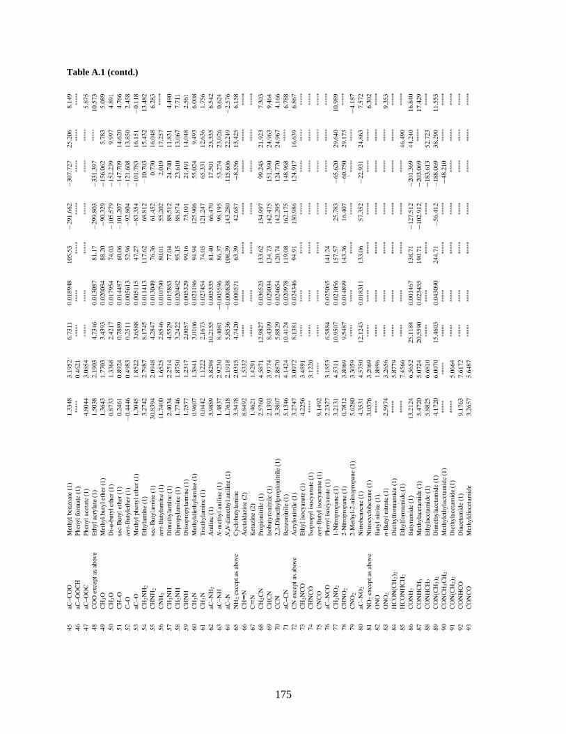
175
Table A.1 (contd.)

176
Table A.1 (contd.)

177
Table A.1 (contd.)

178
Table A.2: Second-order group contribution data (Marrero & Gani, 2001).

179
Table A.2 (contd.)

180
Table A.2 (contd.)

181
Table A.3: Third-order group contribution data (Marrero & Gani, 2001).
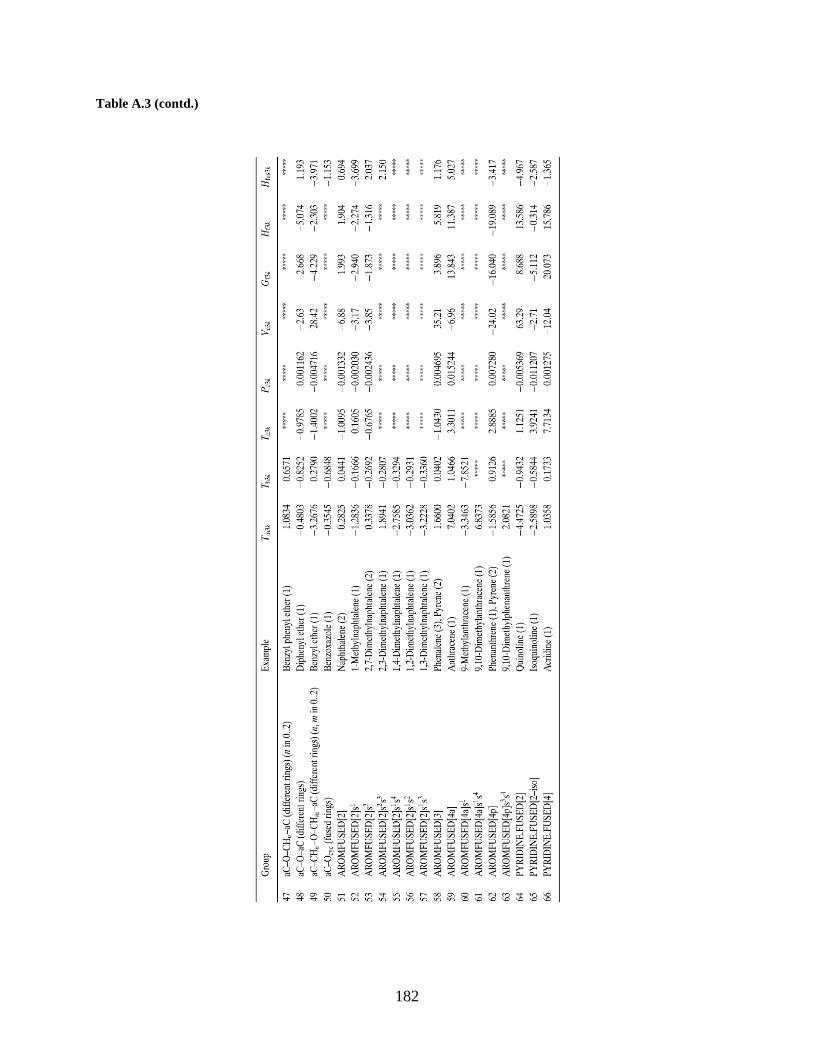
182
Table A.3 (contd.)

183
Table A.4: Property model for each property (Marrero & Gani, 2001)
Table A.5: Value of Adjustable Parameters (Marrero & Gani, 2001)

184
Table A.6: First-order group contribution data (Marrero & Gani, 2002)

185
Table A.6 (contd.)

186
Table A.7: Second-order group contribution data (Marrero & Gani, 2002).

187
Table A.7 (contd.)

188
Table A.8: Third-order group contribution data (Marrero & Gani, 2002).

189
Table A.9: Property Models for properties (Marrero & Gani, 2002).

190
Table A.10: First-order group contributions to the dispersion partial solubility parameter, δd , the polar partial
solubility parameter, δp, and the hydrogen-bonding partial solubility parameter, δhb (Stefanis & Panayiotou,
2008).

191
Table A.10(contd.)

192
Table A.11: Second-order group contributions to the dispersion partial solubility parameter, δd , the polar
partial solubility parameter, δp, and the hydrogen-bonding partial solubility parameter, δhb. (Stefanis &
Panayiotou, 2008)

193
Table A.12: Property Models for estimation of Hansen solubility parameters.
Table A.13: Regressed Parameters for the CI Method (Gani et al., 2005).

194
Table A.14: Classification of Groups (Gani et al., 1991).

195
Table A.15: Rules for generation of acyclic molecules (Gani et al., 1991).

196
Table A.16: Rules for generation of aromatic molecules (Gani et al., 1991).

197
Table A.17: Rules for generation of cyclic molecules (Gani et al., 1991).

198
Appendix B.
Appendix B gives the required literature data for computer aided flowsheet design.
Table B.1: Recommended limits on properties for separation techniques (Jaksland et al., 1995).

199
Table B.2: Available PGs (Alvarado, 2010; d'Anterroches, 2006).
Unit Operation Process-group example
Simple Distillation Column (AB/C)
Solvent Based Azeotropic Separation (cycA/B)
Flash Separation (fAB/CD)
Kinetic Model Based Reactor (rABC/nE/pABCD)
Fixed Conversion Reactor (rABC/nE/pABCD)
Pressure Swing Distillation (swA/B)
Polar Molecular Sieve Based Separation (pmsABC/D)
Molecular Sieve Based Separation (msABC/D)
Liquid Membrane Based Separation (lmemABC/D)
Liquid Adsorption Based Separation (ladsABC/D)
Gas Membrane Based Separation (gmemABC/D)
Pervaporation Based Separation (pervABC/D)
Crystallization Based Separation (crsABC/D)
Liquid Liquid Extraction Based Separation (lleABC/S/SC/AB)
Simple Solid Liquid Separation (slAB/CD)
Absorption (abEAB/eF/EABF/EF)
Ion Exchange Separation (ieABCD/ABC)

200
Table B.3: Rules to denote PGs by invariants through example (d'Anterroches, 2006).

201
Table B.4: Contributions of the simple distillation process groups (d'Anterroches, 2006).

202
Table B.5: Contributions of the extractive process groups (Alvarado, 2010).

203
Table B.6: Pre-calculated values based on driving force approach to design simple distillation columns (Bek-
Pedersen, 2003)

204
Appendix C
Reverse simulation procedure for distillation PGs based on the driving force concept (Bek-
Pedersen, 2003)
The procedure to determine the design parameters of the distillation column in the distillation
process group is as follows:
1. Given a NC component process group.
2. Order the components by relative volatility and identify the key components.
3. Retrieve the maximum DF between the key components, FDimax and the composition of the light
key Dx at its maximum, either from experimental data or VLE calculations.
4. Select the values of product purities or recoveries for the key components, if they are not given
by default 99.5%.
5. If the input composition is between the requested purities for the bottom and top products, then
get the ideal number of stages Nideal for the column from the table of pre calculated values Table
B.6 in Appendix.
6. Set the feed plate location of the column to be NF = (1-Dx)Nideal (plate one is the top plate of the
column).

205
Reverse simulation procedure for kinetic reactor PGs based on attainable region concept
(Glasser et al., 1987) – excerpted from Metzger, Glasser, Glasser, Hausberger, and Hildebrandt
(2007)
Determining the candidate attainable region for a given reaction scheme involves the following
steps: (a) selecting the fundamental processes, (b) choosing the state variables, (c) defining and
drawing the process vectors, (d) constructing the region, (e) interpreting the boundary as the
process flow sheet, and (f) finding the optimum.
(a) Choosing the fundamental process: In this step, the possible physical and chemical
phenomenon possible such as reaction mixing, separation and mass transfer etc. are
selected.
(b) Choosing the state variables: In this step, the state variable that characterize the state of the
system are selected. These variable must be sufficient to describe the dynamics of all the
fundamental process occurring within the system and must include all the variables in the
objective function
(c) Defining and drawing the process vectors: A process vector is one that gives the
instantaneous change in system due to the occurrence of a fundamental process. For
mixing, this vector gives the divergence from the current state, c, based upon the added
state, c*, or v(c, c*) = c* – c. For reactions, vector, r[CA,CB], will give the instantaneous
direction and magnitude of change from the current concentration position. The plug flow
reactor has a defining equation given by 𝑑𝐶
𝑑𝜏= 𝑟(𝑐) and c(t=0) = c0. For a continuous stirred
tank reactor, the same is given by c- c0 = r(c)t.

206
(d) Construction of attainable region: According to Glasser et al. (1987), in order for some
region to be a candidate for the attainable region, it is required that the following necessary
conditions hold true for the Attainable region candidate.
1. The region includes all feed points.
2. No process vectors on the boundary of the region point out of the region
3. No stationary point with mixing as a process exists in compliment to the region.
With these conditions in hand, the general steps to construct an attainable region are as
follows. The attainable region candidate is constructed using a growth approach and a trial
and error method. At each stage the necessary conditions are checked to look for possible
extensions to the region (excerpted from d'Anterroches (2006)).
1. The first step in finding the AR will be to find a CSTR curve PFR trajectory
using the system feed.
2. As the region is not convex, allow mixing between the points. that can be
achieved by the PFR(s). This process is finding the convex hull of the curves
3. Check whether any reaction vectors point out of the surface of the convex hull.
If the reaction vector points out wards over certain regions, then find the
CSTR(s) with feed points in the convex hull that extend the AR the most. If no
reaction vectors point outwards, then check whether the third necessary
condition is met. If they are not met, extend the region using the appropriate
reactor
4. Find the new, enlarged convex hull. If a CSTR lies in the boundary at this stage,
the reaction vectors must point out of the region, and the PFR with feed points

207
on the CSTR will extend the region. Extend the region by finding the convex
hull with these PFR´s included.
5. Repeat the last two steps, alternating between PFR’s and CSTR’s, until no reaction
vectors point out over the region, and necessary third condition is met.
(e) Interpretation of the boundary: Once we have attainable region in hand, to identify the
process flowsheet required to obtain a particular product we trace the path to get to the
particular point of concern. This allows us to determine the correct sequence of
fundamental processes required to achieve the specified product. There is usually only one
path to a particular point on the boundary.
(f) Finding the optimum: With the attainable region fully determined, the optimal value for
any objective function may be determined in a straight forward manner along with the best
process design.
A final point of note is the AR analysis does not guarantee the determination of the complete
attainable region. The analysis is composed of guidelines for the creation of a candidate
attainable region, as no mathematically derived sufficiency conditions exist