integrated analysis of csem, seismic and well log data for...

© 2012 EAGE www.firstbreak.org 43

special topicfirst break volume 30, April 2012

EM & Potential Methods

Integrated analysis of CSEM, seismic and well log data for prospect appraisal: a case study from West Africa.

Lucy MacGregor,2* Slim Bouchrara,1 James Tomlinson,1 Uwe Strecker,1 Jianping Fan,3 Xuefeng Ran4 and Gang Yu4 argue that a significantly more robust interpretation of rock and fluid properties for a pre-drill prospect appraisal can be obtained from the resistivity information acquired by a controlled source electromagnetic (CSEM) survey if seismic and well informa-tion are incorporated. This is illustrated using a case study from offshore West Africa, where a CSEM dataset was acquired in 2009.

I ntegrated analysis of geophysical data can provide valu-able information on reservoir properties and content, on which exploration, appraisal, and development decisions can be based. Traditional reservoir charac-

terization studies integrate seismic data with well-log derived information, using carefully calibrated rock physics relation-ships to relate rock and fluid properties at a log scale, to their surface seismic expression at a geophysical scale. More recently, controlled source electromagnetic (CSEM) data analysis has been integrated into characterization workflows, particularly in cases where the geophysical question of inter-est is ambiguous, or remains unanswered when using a more traditional characterization approach. CSEM provides a measure of subsurface resistivity, which when interpreted in terms of the underlying rock and fluid properties, is a com-plement to seismically derived attributes (e.g., Constable and Srnka, 2007; MacGregor, 2012).

The largest variations in seismic properties such as Vp, Vs, bulk density, acoustic impedance, and Poisson’s ratio often occur at lithology boundaries. In contrast the effect on the seismic properties of a change in fluid is often small. In prin-ciple fluid information can be extracted from seismic data: sometimes this is a successful strategy, however in other situ-ations it is difficult or impossible to do so with certainty. In contrast, electrical resistivity shows a high degree of sensitiv-ity to fluid content. In most hydrocarbon saturated intervals, resistivity is one to two orders of magnitude higher than in the surrounding water saturated sediments. For this reason, downhole resistivity measurements have long provided a key measurement, used by petrophysicists in determining water saturation and fluid properties in a well. The addition of remote measurements of resistivity using CSEM methods

allows the benefits of such information to be utilized away from the wellbore, in conjunction with seismic and other geophysical data.

Analyzing and interpreting seismic or CSEM data to provide a measure of impedance or resistivity is only the first step in an interpretation process. Measurements of physical properties must be further interpreted to determine the underlying rock and fluid properties causing them. This transformation is often non-unique, and subject to uncer-tainty. For example, whereas a zone of high resistivity can be caused by the presence of hydrocarbon fluids, there are many other competing formation types, such as cemented sand-stone, limestones, volcanics, gas hydrates, salt, or coals which could all account for measurements of anomalously high resistivity. Similar uncertainties exist in seismically derived properties. For example AVO and amplitude anomalies may be caused by lithology or thin bed effects rather that fluids, and saturation is often difficult to determine on the basis of seismic data alone.

The most reliable answer to a geophysical question is obtained by using the tool, or combination of tools best suit-ed for the task. Consequently, integrating the resulting data within a rock physics framework provides an Earth model that is consistent with each of the geophysical measurements available, and consistent with the geology of the area under investigation. In this case study, these ideas are applied to the pre-drill appraisal of a prospect offshore West Africa.

Background and surveyThe survey area lies in 2000–2200 m of water in an area dominated by a passive margin rift basin developed since the early Cretaceous. Regionally the basin is characterized by

1 RSI, 2600 South Gessner, Suite 650, Houston, Texas 77063 USA.2 RSI, The Technology Centre, Claymore Drive Bridge of Don Aberdeen AB23 8GD, UK.3 CNODC, CNPC, Beijing, P.R. China.4 BGP, CNPC, Zhuozhou, Hebei Province, 072751, P.R. China.* Corresponding author, E-mail: [email protected]

www.firstbreak.org © 2012 EAGE44

special topic first break volume 30, April 2012


Analysis of the CSEM dataThe interpretation of CSEM data proceeds in stages, starting with simple 1D approaches and gradually adding complex-ity as required to explain the data. The first stage uses a 1D forward modelling approach, aimed at establishing a 1D geoelectric layer profile driven by the known seismic struc-ture/thickness trends encountered in the area, to generate a calibrated background model. Although this approach cannot account for complex or higher dimensional structure, it allows the class of structures to which the data are sensitive, and variations in these structures across the area to be assessed. At this stage any inconsistencies with the expected structure and well-log derived resistivity can be investigated. The degree of electrical anisotropy in the structure can also be assessed and constrained. The results form an important component in the development of inversion approaches and constraints. In this example, initial analysis of the CSEM data demonstrated a high level of electrical anisotropy in the overburden section.

The next stage in the interpretation is to apply a 2.5D inversion. The unconstrained inversion approach seeks a 2D resistivity model that provides a good fit to the acquired data, and which is smooth in a first derivative sense (Constable et al., 1987). Resistivity reconstructions are there-fore as close to a uniform half-space as can be supported by the data. Sharp resistivity contrasts would be expected to be smoothed, whereas the resistivity-thickness product would be accurately estimated. Although this unconstrained approach results in a low resolution image of the resistivity structure, it is a useful first step, allowing the sensitivity of the data to earth structure to be assessed before any a priori constraints are added. In this case the structure and depths to major stratigraphic boundaries are well constrained by

the progradation of upper, middle, and lower slope paleo-depositional environments, with different trap types devel-oped in each (Brownfield and Charpentier; 2006a, 2006b). The survey area is located on the current lower slope and comprises distal deep water fans and channel lobe systems. The late Cretaceous (Maastrichian-Campanian-Santonian) marine turbidite sandstones deposited during the rifting phase are the primary targets. These have already proven to be economic pay zones with sound reservoir quality in adjacent areas, and lie at 2000–3000 m below seabed.

The survey area is covered with a 3D seismic survey providing high resolution structural information. Although there is no well in the immediate vicinity, wells from sur-rounding areas, penetrating the same stratigraphic intervals encountered in the prospect area, are available. These, along with knowledge of the regional geology, were used to construct a background model, and examine the sensitivity of both seismic and CSEM attributes to variations in rock and fluid properties likely to be encountered.

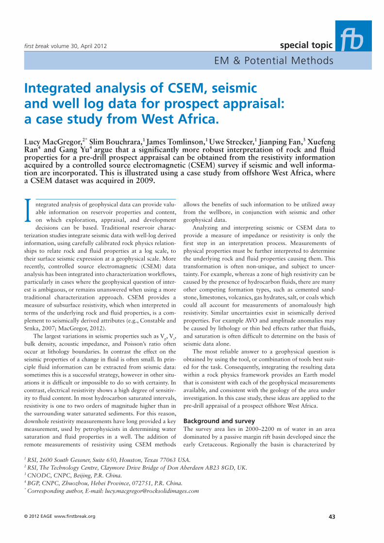
The prospect centred CSEM survey targeted a large four-way dip closure, and was designed to provide high resolution 3D coverage. An array totalling 61 receivers was deployed, and the CSEM source towed along six transmission lines to provide comprehensive in-line and multi-azimuth data cover-age, a requirement to constrain the electrical anisotropy in the section which previous experience in West Africa suggests can be significant. The fundamental frequency of the source was 0.08Hz, with significant power in its harmonics to yield a dataset with rich frequency coverage between the funda-mental and 1.5Hz. Of the 61 receivers deployed, 38 were equipped with magnetic field sensors to allow simultaneous collection of magnetotelluric data during the deployment.

Figure 1 Layout of the prospect specific 3D CSEM survey overlain on seafloor bathymetry. The Campanian (blue) and Santonian (green) prospects are outlined. Receiver locations are shown in yel-low, and CSEM source tow lines in black.




appears to be low compared to the same depth interval outside the seismically mapped prospect extents. A similar effect was observed on the other lines in the survey.

To investigate these features further, the lateral variation in integrated vertical resistivity (corresponding to the trans-verse resistance across an interval of choice) derived from inversion of each line in the survey was co-rendered with a seismic depth slice (Figure 3). The left panel shows resistivity at shallow depths, highlighting the variation in the shallow structure and its correlation with seismic variations. The right panel shows the equivalent integrated vertical resistivity across the prospect interval (Campanian-Santonian) mapped onto a seismic depth slice, taken at 5000 m below sea sur-face. The approximate prospect outlines are shown in grey. The results confirm the observation from Line 1 and 2: the area of the prospect appears to be coincident with a region of low resistivity.

InterpretationTwo conclusions can be drawn from the CSEM data analysis above. Firstly, in the shallow structure (about 500 m–1 km below seafloor) there is a region of high resistivity that was not predicted in the pre-survey analysis. Secondly, and more importantly, within the prospective interval of interest the resistivity mapped appears to be low compared to the same interval outside the prospect extent. However before either conclusion can be considered final, it must be placed in the geological context of the area, and as far as possible a hypothesis for the cause, or causes, of the resistivity effects observed must be established.

coincident seismic data. Seismic structural constraints can be included in the CSEM inversion in order to improve the resolution of the result.

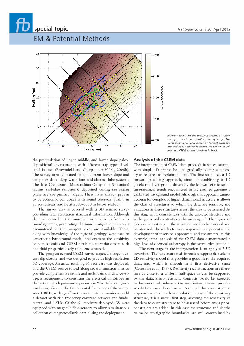
A 2.5D constrained anisotropic inversion approach was applied along each line in the survey. Figure 2 shows the resulting horizontal and vertical resistivity sections along line 1 and line 2 as example. The CSEM derived resistivity has been co-rendered with seismic data, and major stratigraphic boundaries are shown. The inversion was prejudiced to an a priori resistivity of 10 Wm, derived from analysis of the coin-cident magnetotelluric data, below the deepest stratigraphic boundary where CSEM sensitivity is poor, and a break in the smoothness constraint was allowed at this boundary. Apart from this, the inversion was allowed to vary the resistivity freely. The starting model was a pseudo-section derived in the 1D reconnaissance modelling phase.

The horizontal resistivity section is relatively featureless for both lines. In contrast there are pronounced lateral and vertical variations in the vertical resistivity sections. This suggests that the features observed in the vertical resistivity section originate from relatively thin features in the seafloor, which are not well resolved by the data constraining the horizontal resistivity.

Two main features can be seen. Firstly at relatively shallow depths (2.5–3 km below sea surface) there is a zone of high resistivity, which varies laterally along the line. The prospect lies at 5–5.5 km in the below sea surface in the Campanian-Santonian interval. At this level there are clear lateral variations in resistivity along the line. However, for both lines shown in Figure 2, the resistivity at prospect level

Figure 2 Vertical (left) and horizontal (right) resistivity sections along line 1 (top) and line 2 (bottom), co-rendered with seismic data. Red colours correspond to areas of high resistivity. Major stratigraphic boundaries are also shown. Black ticks show the receiver locations at the seafloor and the crossing point of the two lines is marked by the vertical black dashed line. The approximate extent of the seismically mapped prospect is shown by the white arrow.

Picture of low resolution quality, please provide new one




There are a number of possible interpretations of these shallow resistive features. Gas hydrates for example are present in some areas in West Africa (e.g., Cunningham and Lindholm, 2000), and may produce shallow resistivity anomalies such as those observed (e.g., Weitmeyer et al., 2006). However in this case the seismic and well log data from the area suggest an alternative cause. Although there is no well within the survey area itself, a seismic tie line to the nearest well, approximately 70 km to the East of the survey area penetrating the same shallow Tertiary section was analyzed. The resistivity log from this well shows similar high resistivity spikes in the Tertiary section. Detailed analysis of seismic data in the survey area shows morphological features that suggest biogenic carbonate deposits may be the cause of the high resistivity observed, and

Shallow resistivity variationsA region of relatively high resistivity, which varies laterally across the survey area, is observed in the Tertiary section at about 500 m–1 km below mudline. The left panel of Figure 3 shows that areas of high resistivity are present at the northern and southern end of the survey, with a lower resistivity region in between showing an EW trend. Correlation between the seismic and the shallow resistivity features can also be seen in Figure 3. A seismic depth slice has been extracted from the 3D volume available at the depth of the features, and co-rendered with a depth resistivity map interpolated from the 2.5D inversion results. This shows good correlation at the NE end of the survey where the shallow resistor is consistently present.

Figure 3 Lateral variations in vertically integrated resistivity at shallow depth (left panel) and at prospect depths (right panel), mapped onto equivalent seismic depth slices. CSEM receiver lines are overlain (white lines). In the shallow structure the lateral variations in resistivity appear well correlated with the variation in seismic character across the area. At prospect depths, the lateral variations in resistivity observed conform to the results from lines 1 and 2 (Figure 2). The prospects, outlined in grey, appear coincident with a region of low resistivity (green/blue colours).

Figure 4 Resistivity vs acoustic impedance (AI) cross-plots from a representative well in the region. The left panel is colour coded by water saturation. The right panel is colour coded by clay content. Clean reservoir sands show a consistently lower resistivity than either hydrocarbon sands or the surrounding clay rich intervals.

Picture of low resolution quality, please provide new one




tivity zone coincident with the seismically mapped prospect is disappointing, however a plausible geological explanation must be sought before it can be considered conclusive. Two hypotheses were considered:

Hypothesis 1: Tight carbonates of variable thicknessA regional resistive carbonate layer is present at or around the prospect depth, which thins over the prospect. As the layer thins the integrated resistance, to which the CSEM data

indeed carbonates are present in most of the wells in the region. Although these features are not of immediate exploration inter-est, the good correlation with seismic and well log information, and a geologically consistent explanation of their origin, builds confidence in the interpretation of the remaining features.

Resistivity variations at prospect depthOf more interest is the variation in resistivity at prospect depths (Figure 3, right panel). The observation of a low resis-

Figure 5 Synthetic tests used to examine the two hypotheses established to explain the observed data. Left panels: anisotropic resistivity models constructed from well and seismic information. Right panels: Resistivity sections derived from inversion of synthetic data, using the same inversion approach and constraints as applied to the survey data. Top two rows represent hypothesis (1): the variation in resistivity observed is explained by a lateral change in the thickness of a regional resistive carbonate layer. Bottom two rows represent hypothesis (2): The resistivity variations observed are the result of high porosity brine saturated sands in the prospect, giving rise to a lateral variation in resistivity.




a low impedance compared to the surrounding strata, whereas a high resistivity tight carbonate would be expected to be a high impedance feature. However given that neither hypothesis supported the presence of hydrocarbons in this case, no further work was undertaken, and the block was relinquished without drilling.

ConclusionCSEM methods can add valuable information in pre-drill prospect appraisal. In this example the results of CSEM analysis suggested a low resistivity zone coincident with the prospect. However such resistivity information is significantly more robust when interpreted with seismic and well log infor-mation and placed in a regional geological context. In this instance the observed variations could be explained either by the presence of a regional carbonate layer of varying thickness or the presence of good quality sands saturated with brine in the prospect area. Both hypotheses are supported by regional rock physics analysis, and on this occasion neither supports the presence of hydrocarbons in the prospect. Although further work to refine this interpretation could be undertaken, given the high cost of drilling in such a deep water area, as a result of the integrated analysis the block was dropped.

AcknowledgementsWe are grateful to BGP, CNODC, and CNPC for permission to publish this case study. We also thank Franklin Ruiz, Josh Hataaja, and Skander Hili for their valuable input to the project.

ReferencesBrownfield, M.E. and Charpentier, R.R. [2006a,] Geology and Total

Petroleum Systems of the West-Central Coastal Province (7203),

West Africa. US Geological Survey Bulletin, 2207-B.

Brownfield, M.E. and Charpentier, R.R. [2006b] Geology and Total

Petroleum Systems of the Gulf of Guinea Province of West Africa

(7183). US Geological Survey Bulletin, 2207-C.

Constable, S.C., Parker, R.L. and Constable, C.G. [1987] Occam’s inver-

sion: A practical algorithm for generating smooth models from EM

sounding data. Geophysics, 52, 289–300.

Constable, S. and Srnka, L.J. [2007] An introduction to marine controlled

source electromagnetic methods for hydrocarbon exploration.

Geophysics, 72, WA3-WA12.

Cunningham, R. and Lindholm, R.M. [2000] Seismic evidence for wide-

spread gas hydrate formation, offshore West Africa. In Mello, M.R.

and Katz, B.J. (Eds.) Petroleum systems of South Atlantic margins.

AAPG Memoir, 73, 93–105.

MacGregor, L.M. [2012] Integrating seismic, CSEM and well log data

for reservoir characterization. The Leading Edge, 31(3), 258–265.

Weitmeyer, K.A., Constable, S.C., Key, K.W. and Behrens, J.P. [2006] First

results from a marine controlled-source electromagnetic survey to

detect gas hydrates offshore Oregon. Geophysical Research Letters,

33. L03304, doi:10.1029/2005GL024896.

are sensitive, reduces resulting in the observed low resistivity zone. This would be consistent with the observation from wells in the region that carbonates are present across most of the section at various locations.

Hypothesis 2: Laterally varying resistivity within the prospect intervalThe resistivity of the prospect interval varies laterally and is lower over the prospect than outside it. Support for this hypothesis comes from analysis of over 40 wells in the region, penetrating Campanian-Santonian reservoir sands. Cross-plots of the properties from a nearby well with sig-nificant hydrocarbon saturation is shown in Figure 4, colour coded by saturation and clay content. The data are character-ized by a horizontal trend corresponding to the background shales and silty sands. Their resistivity is almost constant at around 1 Ωm, consistent with the CSEM inversion results in the overburden. The hydrocarbon saturated sands are represented by the cyan colour on the right plot and the red colour on the left plot. They are, as expected, more resistive than both brine-saturated sands and background shales/silty sands. However clean brine saturated sands show a signifi-cantly lower resistivity than the hydrocarbon saturated and shaley sands. This type of response is typical for the region, and a pattern that can be related to what is observed in the target region on CSEM analysis results. The low resistivity region within the prospect area could be explained by the presence of high quality reservoir sands within the prospect, which are saturated with brine.

To test these hypotheses further, anisotropic resistivity models along Line 1 were constructed representing each. From these, synthetic CSEM data were generated and con-taminated with noise levels consistent with those observed in the survey data. These synthetic data were then inverted using the same approach as applied to the survey data. This approach allows the effect on the result of the inversion approach and constraints applied to be assessed. The results are shown in Figure 5.

Comparing the results of the synthetic inversion (Figure 5) with the results of the inversion of the survey data shown in Figure 2, it is clear that both hypotheses give a result that is consistent with the CSEM data analysis results. The observed resistivity variation could be caused by either a regional resis-tive carbonate layer that thins over the prospect, or by good quality reservoir sands within the prospect that are saturated with brine, giving rise to a lateral variation in resistivity. CSEM data are primarily sensitive to the transverse resist-ance (vertically integrated resistivity) and therefore a change in thickness of a layer of constant resistivity will have much the same effect on the data as a lateral change in resistivity of a constant thickness layer. Seismic data analysis could be used to distinguish these possibilities: a good quality reservoir sand of high porosity would be expected to have

integrated analysis of csem, seismic and well log data for...

Documents