Integrate Learning and Control in Queueing Systems withUncertain Payoff

Wei-Kang Hsu, Jiaming Xu, Xiaojun Lin, Mark R. Bell

Purdue University

Abstract

We study task assignment in online service platforms where un-labeled clients arrive according to astochastic process and each client brings a random number of tasks. As tasks are assigned to servers,they produce client/server-dependent random payoffs. The goal of the system operator is to maximizethe long-term average payoff subject to the servers’ capacity constraints. However, both the statisticsof the dynamic client population and the client-specific payoff vectors are unknown to the operator.Thus, the operator must design task-assignment policies that integrate adaptive control (of the queueingsystem) with online learning (of the clients’ payoff vectors). A key challenge in such integration is howto account for the non-trivial closed-loop interactions between the queueing process and the learningprocess, which may significantly degrade system performance. We propose a new utility-guided onlinelearning and task assignment algorithm that seamlessly integrates learning with control to address suchdifficulty. Our analysis shows that, compared to an oracle that knows all client dynamics and payoffvectors beforehand, the payoff gap of our proposed algorithm decreases as O(1/V ) + O(

√logN/N),

as a parameter V of the algorithm and the average number N of tasks per client increase. Throughsimulations, we show that our proposed algorithm significantly outperforms a myopic matching policyand a standard queue-length based policy that does not explicitly address the closed-loop interactionsbetween queueing and learning.

1 Introduction

Thanks to the advance in communication and computing, new generations of online service platformshave transformed the business models in many domains, from online labor market of freelance work (e.g.,Upwork [Upw]), online hotel rental (e.g., Airbnb [Air]), online education (e.g., Coursera [Cou]), crowd-sourcing (e.g., Amazon Mechanical Turk [Ipe10]), to online advertising (e.g., AdWords [AdW]) and manymore. By bringing unprecedented number of clients and service providers together, these online serviceplatforms greatly increase access to service, lower the barrier-to-entry for competition, improve resourceutilization, reduce cost and delay, and thus enhance the overall well-being of society and our daily life.

Motivated by these online service platforms, in this paper we are interested in learning and controlproblems in queueing systems with uncertain agent dynamics and uncertain payoffs. Note that a key controldecision in operating such online service platforms is how to assign clients to servers to attain the maximumsystem benefit. Such decisions are challenging because there often exist significant uncertainty in bothagent payoffs and agent dynamics. First, there is significant uncertainty in the quality, i.e., payoff, of aparticular assignment between a client (needing service) and a server (providing service). For example,in online ad platforms, when an ad from a particular ad campaign is displayed in response to a searchrequest for a given keyword, the click-throughput rate is unknown in advance [CJS15]. Similarly, in crowd-sourcing, the efficiency of completing a particular task by a given worker is unknown a priori [KOS11a,

1

KOS13, KOS11b, KO16]. Second, the population of agents (i.e., clients or servers) is often highly dynamic.For example, ad campaigns arrive and depart constantly in online ad platforms [TS12]; so do requestorsin crowd-sourcing. The statistics of such arrivals and departures are often unknown beforehand, resultinginto uncertain queueing dynamics. Therefore, the operator of these platforms must not only continuouslylearn the payoffs associated with each new agent, but also adaptively control the assignment and resourceallocation in response to the uncertain arrival/departure dynamics. Thus, it is imperative to study both onlinelearning (of uncertain payoffs) and adaptive control (of uncertain queueing dynamics) in a unified frameworkto achieve optimal performance in such a dynamic and uncertain environment.

Prior Work That Studies Learning and Queueing Seperately: Prior studies on online service plat-forms often treat the optimal learning problem and the adaptive control problem separately, and as a resultmay produce significantly sub-optimal results when there is uncertainty in both agent dynamics and agentpayoffs. From the learning side, multi-armed bandits (MAB) [LR85, ACBF02, GGW11, BCB+12] havebeen extensively used to model online decision problems with uncertain payoffs. In a classical MAB formu-lation, a client has a sequence of jobs that need to be assigned, one at a time, to servers with uncertain payoffs(corresponding to “arms” in the MAB literature). The key question is how to balance exploitation (using thecurrently-known best server) and exploration (finding out which server is the best). However, these studiesusually focus on a static setting, without considering the uncertainty in queueing dynamics. For example,most stochastic bandit [LR85, ACBF02], Markovian bandit [Git79, Whi88] and adversarial bandit problems[ACBFS02] assume only one client. Although bandits with dynamic arms (e.g., the open-bandit processes)[LY88, WZ13, Whi81] allow the number of servers/arms to follow a Markov process, the statistics of theMarkov chain must be known in advance. Similarly, although contextual bandits (as in the studies of onlinead [CJS15, JS13, PO07, BLS14, LZ08] and crowd-sourcing [JNN14, TTSRJ14]) may be interpreted as al-lowing arriving jobs of multiple types, the label (i.e., context) of each job must be known in advance. Thus,they cannot be used when there is a dynamic population of clients with unknown labels. More recently, thework in [KNJ14, NKJ16, GKJ12, AMTS11, LEGJP11, LPT13, CP15, LCS15, SRJ17, BTZ15] considers amore-general multi-player setting and combines learning (of agent features) with matching, combinatorialoptimization, and/or consensus decisions. However, such results still assume a static setting with a fixednumber of agents, and thus do not account for the queueing dynamics due to agent arrivals and departuresin practical online service platforms. In this sense, they can at best be viewed as a myopic solution for asnapshot of the system in time. As we will elaborate in Section 3, using such a myopic solution from a staticsetting could lead to substantially lower levels of system performance when the agent dynamics are takeninto account.

At the other end of the spectrum, the operation of online service platforms has been studied as a stochas-tic or adversarial matching/queueing problem. Adaptive control policies under uncertain dynamics havebeen provided, e.g., for online ad [TS12, FKM+09, CZL08, AHL13, ZCXL13] and/or queueing networksin general [TE92, NML05, Chi04, ES05, LS05, LSS06, LSS08], to maintain system stability, maximizepayoff, and/or minimize cost and delay. However, these studies usually assume that the payoff vectors of theclients are known. In practice, the payoff vectors of new clients are often unknown. These adaptive controlpolicies will break down without this crucial piece of information. Recently, there have been studies thatcombine the notion of learning with queueing [HLH14, HZCL16]. However, the focus of these studies is inlearning the arrival rates. Thus, they have not considered uncertain payoffs.

Our Contributions: In constrast to the above lines of work that study learning and queueing separately,in this paper we focus on the following queueing system model that incorporates uncertainty in both agentdynamics and payoffs. Note that in many online service platforms, the operator often has enough aggregateinformation on the servers’ features, and servers arrive at and depart from the system at a slower time scalethan clients [JKK16, MX16, JKK17]. Thus, in this work we assume that there are a fixed number of servers,while clients of multiple classes arrive to the system with unknown arrival rates. Each client brings a randomnumber of tasks. Associate with each class is a payoff vector over all servers. As the tasks of a client are

2

assigned to different servers, they produce random payoff feedback with mean given by the underlyingclass-dependent payoff vector. However, neither the class label of a client nor its payoff vector is knownto the operator. Thus, the operator has to learn the payoff vector of a new client from the random payofffeedback. We then develop a utility-guided online learning and task assignment algorithm that can achievenear-optimal system payoff even compared to an “oracle” that knew the statistics of client dynamics and allclients’ payoff vectors beforehand. Specifically, we will show that the gap between the long-term averagepayoff achieved by our proposed algorithm and the upper-bound payoff of the “oracle” is at most the sum oftwo terms, one of which is of the order O(1/V ) where V is a parameter of the proposed algorithm that canbe taken to a large value; the other is of the order O(

√logN/N) where N is the average number of tasks

per client.There are a few recent studies in the literature that also attempt to integrate learning and queueing

[JKK16, MX16, JKK17, BM15, SGMV17]. Compared to these related studies, our work makes a numberof new contributions. Note that a key challenge in integrating learning with queueing is the non-trivialclosed-loop interactions between the queueing process and the learning process. Specifically, excessivequeueing, which can be caused by both agent arrivals/departures and task assignments/completion, leadsto both delay in observing the payoff feedback and a slow-down of the learning process of the uncertainpayoffs. Ineffective learning, in turn, leads to suboptimal assignment decisions based on inaccurate payoffestimates, which increases queueing delay and lowers system payoff under uncertain agent dynamics. Suchclosed-loop interactions, if not properly managed, can produce a vicious cycle that severely degrades theoverall system performance (see further discussions in Section 3). Prior work in [JKK16, MX16, JKK17]attempts to deal with this closed-loop interactions by essentially decoupling queueing from learning. Forexample, the policies there explicitly divide exploration (where learning occurs) and exploitation (wherequeueing and control occur) into two stages. However, in doing so they require strong assumptions onprior knowledge of uncertainty, such as the knowledge of the type-dependent payoff vectors, the numberof tasks per client, and/or the arrival statistics of the clients (see further comparison in Section 3). Whilethese assumptions simplify the analysis, they become highly restrictive when such prior knowledge is eitherunavailable or inaccurate.

In contrast, our study contributes to the understanding of the aforementioned closed-loop interactions(between queueing and learning) by introducing new ideas in both algorithm design and performance anal-ysis. In terms of algorithm design, we develop new algorithm (with provable performance guarantees) thatrequires no prior knowledge of the class-dependent payoff vectors, arrival statistics, nor the number of tasksper client. Further, it does not employ a separation between the exploration stage and the exploitation stage,but instead seamlessly integrates exploration, exploitation, and dynamic assignment at all times. To accom-plish this goal, our proposed algorithm employs a novel form of utility-guided fair assignment combinedwith Upper-Confidence-Bound (UCB)-style [ACBF02] payoff estimates. A desirable feature of this utility-guided algorithm is that it eliminates the delay in the payoff feedback due to task-queues at servers, and thussignificantly reduces the negative impact in the direction from queueing to learning (see Section 4 for moredetailed discussions).

Then in terms of performance analysis, we provide new analytical techniques to prove the performanceguarantees of the proposed algorithm. In contrast to the analyses in [JKK16, MX16, JKK17] that rely on aseparation between exploration and exploitation, our analysis is more involved because it needs to explictlyaccount for the closed-loop interactions between the queueing process and the learning process at all time.Specifically, we develop a novel Lyapunov-based drift analysis that carefully captures both the impact of thepayoff estimation errors on the queueing dynamics, and the impact of congestion on the rate of learning foreach client’s payoff vector (see Section 6 for more detailed discussions). This refined analysis thus providesnew and non-trivial insights on how to choose the parameters of the algorithm to achieve the desirableperformance guarantees.

The rest of the paper is organized as follows. The system model is defined in Section 2, and related

3

𝜇1

𝜇2

𝜇𝐽

…

𝜆

𝑁(=? )

𝐶𝑖1∗ (=? )

𝐶𝑖2∗ (=? )

Server 1

Server 2

Server 𝐽

𝐶𝑖𝐽∗ (=? )

1

𝑁(=? )

[𝜌𝑖]

Clients

𝑙

Figure 1: Uncertain client dynamics and payoffs.

approaches are discussed in Section 3. We then present our new algorithm and main analytical results inSection 4. Simulation results are shown in Section 5, and key proofs are presented in Section 6. Finally, weconclude and discuss possible future directions.

2 System Model

We model an online service platform as a multi-server queueing system that can process tasks from a dy-namic population of clients, as shown in Fig. 1. Time is slotted. At the beginning of each time-slot t, anew client arrives with probability λ/N , independently of other time-slots. Upon arrival, the client carriesa random number of tasks that is geometrically distributed with mean N . Note that in this way the totalrate of arriving tasks is λ. A client leaves the system once all of her tasks have been served. We assumethat each client must belong to one of I classes. There is a probability distribution [ρi, i = 1, ..., I] with∑I

i=1 ρi = 1, such that a newly-arriving client belongs to class i with probability ρi, independently of otherclients. Let S = {1, 2, . . . , J} denote the fixed set of servers. Each server j ∈ S can serve exactly µj tasksin a time-slot. (We will briefly discuss in Section 7 how to treat the case when the service is random.) Letµ =

∑Jj=1 µj .

Each class i is associated with a payoff vector [C∗ij , j = 1, ..., J ], where C∗ij is the expected payoff whena task from a class-i client is served by server j. Note that all tasks associated with a client have the samepayoff vector. However, the arrival rate λ, the class distribution ρi, the expected number N of tasks perclient, the class label of a new client, her total number of tasks, and her payoff vector are all unknown tothe system. The system does know the identity of the servers and their service rates µj . Another importantquantity that the system can learn from is that, after a task from a client is served by server j, the systemcan observe a noisy payoff of the task. Conditioned on the task being from a class-i client, this noisy payoffis assumed to be a Bernoulli random variable with mean C∗ij , (conditionally) independently of other tasksand servers. (The Bernoulli assumption is used here for ease of exposition. We expect that it would bestraightforward to extend the results of this paper to more general distributions.)

The goal of the system is then to use the noisy payoff feedback to learn the payoff vectors of the clients,and to assign their tasks to servers in order to maximize the total system payoff. Such decisions must beadaptively made without knowing the statistics of the client arrivals and departures. At each time-slot t, letn(t) be the total number of clients in the system (including any new arrival at the beginning of the time-slot).Let plj(t) be the expected number of tasks from the l-th client that are assigned to server j in this time-slot,l = 1, ..., n(t). Further, let i(l) denote the underlying (but unknown) class of the l-th client. Then, thedecision at time t of a policy Π essentially maps from the current state of the system (including all payofffeedback observed before time t) to the quantities plj(t). The average payoff of such a policy Π is given by:

R(Π) = limT→∞

1

T

T∑t=1

J∑j=1

E

n(t)∑l=1

plj(t)C∗i(l),j

. (1)

4

In contrast, note that if an “oracle” knew in advance the statistics of the arrival and departure dynamics (i.e.,λ, ρi and N ), as well as the class label and payoff vector of each client, one can formulate the followinglinear program:

R∗ = max[pij ]≥0

λ

I∑i=1

ρi

J∑j=1

pijC∗ij (2)

subject to λI∑i=1

ρipij ≤ µj for all servers j, (3)

J∑j=1

pij = 1 for all classes i, (4)

where pij is the probability that a task from a class-i client is assigned to server j. It is not difficult to showthat R∗ provides an upper bound for the average payoff R(Π) under any policy Π [JKK16, JKK17]. Thus,our goal is to achieve a provably-small gap R∗ −R(Π).

3 Related Approaches in the Literature and Their Weakness

Before we present our solution to this problem, we briefly overview approaches to related problems inthe literature and discuss why they cannot be used to solve the problem that we introduced in Section 2.First, the work in [JKK16, JKK17] also studies how to maximize the average payoff for a system withunknown client types. (The notion of “type” in [JKK16, JKK17] is comparable to “class” in this paper,while “worker” is comparable to “client” in this paper.) However, there are a number of crucial differences.In [JKK16, JKK17], the expected payoff vector of each type is assumed to be known in advance. Further,the theoretical results in [JKK16, JKK17] assume that the policy knows the “shadow prices,” which in turnrequires that the statistics of the client dynamics (i.e., λ, ρi and N ) are known in advance. Moreover, thepolicies in [JKK16, JKK17] explicitly divide exploration (where learning occurs) and exploitation (wherequeueing and control occur) into two stages. In order to control the length of the exploration stage, thesepolicies require prior knowledge of the total number of tasks for each client. In contrast, in our model neitherthe payoff vector for each type (i.e., each “class” in this paper) nor the client arrival/departure statistics areknown to the system. As a result, the theoretic policies in [JKK16, JKK17] are not applicable in our setting.Although [JKK17] also provides a heuristic policy that uses queue length to replace the shadow price, notheoretical performance guarantee is proved. Moreover, this heuristic policy requires that the unused serviceof the servers can be queued and utilized later. Since our model does not allow such queueing of unusedservice, we cannot use this heuristic policy either. One could argue that, after the system has been operatedin a stationary setting for a long time, the operator may eventually be able to learn the arrival/departurestatistics and the class-dependent payoff vectors, in which case the theoretic policies in [JKK16, JKK17]could then be used (although acquiring such knowledge would require highly non-trivial learning proceduresfor estimating both the clients’ payoff vectors and their underlying classes.) Still, the setting studied in thispaper, as well as the adaptive algorithm that we will develop, will be important both for the early phaseof the system operation, and when the class composition or arrival/departure statistics experience recentchanges. Finally, note that the work in [MX16] also assumes the knowledge of the payoff vectors for alltypes in advance and divides exploration and exploitation into distinct stages, although [MX16] does notaim to maximize the system payoff as in this paper.

Myopic Matching: A second line of related work is the multi-player MAB formulation in [KNJ14,NKJ16, GKJ12, AMTS11, LEGJP11, LPT13, CP15, SRJ17, BTZ15], which is also a common way in theliterature to study online learning in a two-sided system, where clients and servers with unknown payoffs

5

1

1

𝜆

𝑁=1.2

𝑁0.9

Server 1

Server 2

1

𝑁

Class 1

0.1

0.3

0.9

1/2

1/2

Clients

Class 2

Figure 2: Myopic matching is suboptimal.

need to be matched to maximize the system payoff. However, this class of work assumes that both the clientpopulation and the server population are fixed. In contrast, in our model the client population is constantlychanging. Thus, the multi-player MAB solution can at best be viewed as a myopic solution for a snapshot ofour system in time. It is not difficult to envision that such a myopic matching strategy (for each snapshot intime) is sub-optimal in the long run with client dynamics. Indeed, as illustrated below, this sub-optimalityexists even when the payoffs vectors are known in advance!

Example (Myopic matching is suboptimal): Assume two servers, each of service rate µj = 1 as shownin Fig. 2. There are two classes, and a new client belongs to one of the two classes with equal probability0.5. The payoff vectors of the two classes are [0.9 0.1] and [0.9 0.3], respectively. Assume N = 100 andλ/N = 1.2/N . It is easy to see that the optimal solution should assign all class-1 tasks to server 1, 2/3of class-2 tasks to server 1, and the rest 1/3 of class-2 tasks to server 2. The resulting optimal payoff is0.6 ∗ 0.9 + 0 ∗ 0.1 + 0.4 ∗ 0.9 + 0.2 ∗ 0.3 = 0.96. However, if a myopic matching strategy is used, withclose-to-1 probability two tasks will be assigned at each time, one of which will have to be assigned to server2. Thus, the overall payoff is approximately upper-bounded by 1.2 ∗ (0.9 + 0.3)/2 = 0.72. As we can see,the myopic matching strategy focuses too much on maximizing the current payoff, and as a result sacrificesfuture payoff opportunities. Naturally, if the class labels and payoff vectors are unknown and need to belearned, a similar inefficiency will incur.

Queue-Length Based Control: The above example clearly illustrates the need to cater to uncertain clientdynamics in the system. In the literature, a third line of related work uses queue-length based contol tobalance current payoff with long-term payoff in the presence of uncertain arrival/departure dynamics [TE92,NML05, Chi04, ES05, LSS06]. This line of work usually assumes that each client’s payoff vector is known.By building up queues of unserved tasks at the servers, one can use the queue length qj at server j asa “shadow price” that captures the congestion level at the server. The system operator then adjusts eachclient’s payoff parameter C∗ij to C∗ij − qj/V with a proper choice of V , and assigns the next task to theserver with the highest adjusted payoff. When the payoff vector of each client is known in advance, thistype of queue-length based control can be shown to attain near-optimal system payoff when the parameterV is large [TS12], although the length of the server-side queues also grows with V .

However, when the payoff vector of each client is unknown, such a queue-length based control leads tocomplicated closed-loop interactions between queueing and learning. In one direction, queueing degradeslearning in at least two ways. First, because the operator only learns the noisy payoff of a task after the taskis served, excessive server-side queues (esp. when V is large) not only delay the service of the tasks, but alsodelay the payoff feedback. As a result, the learning of the clients’ uncertain payoff vectors is also delayed.(We will refer to this effect as the “learning delay.”) Second, because all clients compete for the limitedserver capacity, the learning process of some clients will inevitably be slowed down, which also results inpoor estimate of their payoff vectors. (We will refer to this second effect as the “learning slow-down.”) Then,in the opposite direction, ineffective learning in turn affects queueing because assignment decisions have tobe made based on delayed or inaccurate payoff estimates. Such sub-optimal decisions not only lower systempayoff, but also increase queueing delay. Together, the above closed-loop interactions between queueing andlearning will produce complex system dynamics which, if not designed and controlled properly, can severely

6

degrade system performance. Indeed, as we will demonstrate in Section 5, a straightforward version of suchqueue-length based control will lead to lower system payoff when combined with online learning.

Online Matching: There is a fourth line of related work on online matching that also aims to addressuncertainty in future client dynamics (albeit in an adversarial setting) [AHL13, CZL08, FKM+09, ZCXL13].However, similar to queue-length based control, such studies typically do not deal with payoff uncertaintyeither.

Finally, although [BM15] and [SGMV17] also study the integration of learning and control, they eitherallow only a small system with two types of clients and two servers [BM15], or have to use an exponentialnumber of virtual queues to approach optimality [SGMV17]. In contrast, in this work we aim to developcomputationally-efficient algorithms that can be implemented even for large systems.

In summary, it remains an open question how to seamlessly integrate online learning with adaptivecontrol when there is uncertainty in both client dynamics and payoff vectors, and how to account for thecomplex closed-loop interactions between queueing and learning. Below, we will propose our new algorithmand analytical techniques that address these difficulties.

4 Dynamic Assignment with Online Learning under Uncertainties

In this section, we present a new algorithm that seamlessly integrates online learning with dynamic taskassignment. Somewhat analogously to the idea of queue-length based control [TE92, NML05, Chi04, ES05,LSS06], our new algorithm also uses some form of backlog in the system as a congestion indicator to guidethe task assignment decisions. However, recall that when a queue-length based control policy uses the lengthof the task-queue at each server as the “shadow price,” it produces complex closed-loop interactions betweenqueueing and learning (including the issues of “learning delay” and “learning slow-down”). To circumventthis difficulty, we instead eliminate the task-queues at the servers, and thus eliminate the “learning delay”altogether. This is achieved by controlling the number of tasks assigned to each server j at each time-slotto be always no greater than its service rate µj . However, without the server-side task-queues or “shadowprices”, we need another congestion indicator to guide us in the dynamic assignment of tasks. Here, wepropose to rely on the number of backlogged clients in the system. Specifically, we use the solution to autility-maximization problem (that is based on the current number of backlogged clients in the system) tohelp us trade-off between the current and future payoffs. The parameters of the utility-maximization problemare carefully chosen to also control the “learning slow-down” of all clients in a fair manner. We note thatthe structure of our proposed utility-guided algorithm has some similarity to that of flow-level congestioncontrol in communication networks [LSS08, DLK01, FFL+01, Ye03, BM01], where a fair utility-optimalcongestion controller is shown to ensure system stability (i.e., the number of clients in the system will notapproach infinity). However, the focus there is only on the system stability, but not the system payoff.Further, there is no online learning of uncertain parameters. To the best of our knowledge, our work is thefirst in the literature that uses utility-guided adaptive control policies with online learning to optimize systempayoff.

4.1 Utility-Guided Dynamic Assignment with Online Learning

We present our algorithm in Algorithm 1. At each time-slot t, the algorithm operates in three steps. Step 1generates an estimate [C lj(t)] of the payoff vector for each client l based on any previous payoff feedback(Lines 4-7). Note that n(t) is the current number of clients in the system, including any newly-arrivingclient. For each client l = 1, ..., n(t), if no task of this client has been assigned to server j yet, we setC lj(t) = 1 (Line 6); otherwise, we use a truncated Upper-Confidence-Bound (UCB) estimate [ACBF02] to

7

Algorithm 1: Utility-Guided Dynamic Assignment with Online Learning

1 For every time slot t:2 Update the total number of clients n(t) (including newly arriving clients)3 Step 1: Form UCB-style payoff estimates4 for l = 1 : n(t) do5 for j = 1 : J do6 if hlj(t− 1) = 0 then C lj(t)← 1;7 else Set C lj(t) according to (7) ;

8 Step 2: Assign [plj(t)] as the solution to the following optimization problem9

max[plj ]≥0

n(t)∑l=1

1

Vlog

J∑j=1

plj

+J∑j=1

plj(Clj(t)− γ)

(5)

sub ton(t)∑l=1

plj ≤ µj , for all servers j ∈ S. (6)

10 Step 3: Assign tasks and obtain payoff feedback11 Initialize to zero the number of tasks from client l to be assigned to server j, i.e., Y l

j (t) = 0.12 for j = 1 : J do13 for ν = 1 : µj do14 Choose a client l∗ randomly such that the probability of choosing client l is equal to

plj(t)/µj . Assign one task from client l∗ to server j and let Y l∗j (t)← Y l∗

j (t) + 1 ;

15 for l = 1 : n(t) do16 for j = 1 : J do17 Observe Y l

j (t) number of Bernoulli noisy payoffs

X lj(t, 1), . . . , X l

j

(t, Y l

j (t))

i.i.d.∼ Bern(C∗i(l),j

);

18 hlj(t)← hlj(t− 1) + Y lj (t) ;

19 hl(t) =∑J

j=1 hlj(t) ;

20 Clients with no remaining tasks leave the system.

generate C lj(t) (Line 7):

C lj(t) = min

{Clj(t− 1) +

√2 log hl(t− 1)

hlj(t− 1), 1

}, (7)

where hlj(t−1) is the number of tasks from client l that have previously been assigned to server j before the

end of the (t− 1)-th time-slot and hl(t− 1) =∑J

j=1 hlj(t− 1); C lj(t− 1) is the empirical average payoff

of client l based on the received noisy payoff feedback for server j until the end of the (t− 1)-th time-slot:

Clj(t− 1) =

1

hlj(t− 1)

t−1∑s=1

Y lj (s)∑r=1

X lj(s, r)

8

with Y lj (s) denoting the number of tasks from client l served by sever j at time s, andX l

j(s, 1), . . . , X lj

(s, Y l

j (s))

denoting the received noisy payoff feedback in time-slot s. Since the true payoffs C∗ij’s are within [0, 1],we truncate the UCB estimate at threshold 1 in (7). Then, Step 2 solves a maximization problem (Line9), subject to the capacity constraint of each server, to obtain the values of plj(t), which corresponds to theexpected number of new tasks of client l to be assigned to server j in time-slot t. The objective (5) can beviewed as the sum of some utility functions over all clients. The parameter γ in (5) is chosen to be strictlylarger than 1, and V is a positive parameter. Finally, Step 3 determines the exact number Y l

j (t) of tasks fromclient l that are assigned to server j (Lines 12-14). The values of Y l

j (t) are randomly chosen in such a way

that (i) each server j receives at most µj tasks, i.e.,∑n(t)

l=1 Ylj (t) ≤ µj ; and (ii) the expected value of Y l

j (t)

is equal to plj(t). The tasks are then sent to the servers and new noisy payoffs are received (Lines 15-19).Before we present our analytic results, we make several remarks on the design of our proposed algorithm.Seamless Integration of Learning and Control: First, recall that the policies in [JKK16, MX16, JKK17]

seperate exploration and exploitation into distinct stages. Further, they assume prior knowledge of class-dependent payoff vectors, the total number of tasks per client, and/or “shadow prices.” In contrast, our algo-rithm does not require such prior knowledge at all, and it seamlessly integrates exploration and exploitationin every time-slot.

Zero Learning Delay: Second, note that by Step 3 of the algorithm, the number of assigned tasks toeach server j is no more than the service rate µj . Since server j can serve exactly µj tasks per time-slot, thisimplies that there is no longer any “learning delay,” i.e., all payoff feedback will be immediately revealed atthe end of the time-slot.

The Importance of Fairness: Third, if we removed the logarithmic term in (5) and set γ = 0, then themaximization problem in (5) would have become a myopic matching policy that maximized the total payoffin time-slot t based on the current payoff estimates. However, as we have seen from the counter examplein Section 3, such a myopic matching policy focuses too much on the current payoff, and as a result canunderperform for the long-term average payoff. Instead, the logarithmic term in (5) serves as a concaveutility function that promotes fairness [LSS08, DLK01, FFL+01, Ye03, BM01], so that even clients withlow payoff estimates can still receive some service (i.e.,

∑Jj=1 p

lj(t) is always strictly positive). This fairness

property is desirable in two ways. First, it has an eye for the future (which is somewhat related to the fact thatfair congestion-control ensures long-term system stability [BM01]), so that we can strike the right balancebetween current and future payoffs. Second, it also controls the learning slow-down of all clients in a fairmanner. Specifically, thanks to this fairness property, we can show that the “learning rate” of each clientbased on imprecise payoff estimates will not be too far off from the “learning rate" of the client based on itstrue payoff vector (see detailed discussions in Section 6.5), which constitutes a crucial step in our analysiswhen we bound the payoff loss due to errors of the payoff estimates.

Parameter Choice: Fourth, the choice γ > 1 in (5) and the truncation of the UCB estimates in (7) alsoplay a crucial role in achieving near-optimal system payoff. Note that if γ = 0, then every client l will havethe incentive to increase

∑Jj=1 p

lj(t) by utilizing as many available servers as possible, even when the server

payoff is very close to zero. In contrast, as can be seen again from the counter example in Section 3, in manysettings the optimal policy must restrict some clients to only use the high-payoff servers (see, e.g., class-1clients in the example). Hence, such an aggressive approach may lead to suboptimal performance. Instead,by choosing γ > 1 ≥ C lj(t), the second term inside the summation in (5) becomes negative. As a result,a low-payoff server will only be picked if

∑Jj=1 p

lj(t) is sufficiently small (and thus the derivative of the

logarithmic term, which is equal to 1/[V∑J

j=1 plj(t)], is sufficiently large). This feature leads to an inherent

“conservativeness” of our algorithm. Not surprisingly, we will see that the choice of γ is also crucial in ouranalysis, specifically in Section 6.2 and Section 6.5.

Complexity: Last but not least, the maximization problem in Step 2 is a convex program and can be

9

0 1 2 3 4Time 104

0

0.2

0.4

0.6

0.8

1Av

erag

e pa

yoff

Upper bound Algorithm 1, V = 21 Algorithm 1, V = 2 Queue-length based policy, V= 100 Queue-length based policy, V= 2 Myopic matching

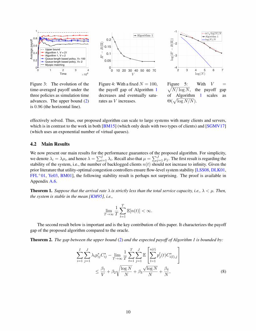
Figure 3: The evolution of thetime-averaged payoff under thethree policies as simulation timeadvances. The upper bound (2)is 0.96 (the horizontal line).

0 10 20 30 40 50 60 700

0.05

0.1

0.15

0.2

Figure 4: With a fixedN = 100,the payoff gap of Algorithm 1decreases and eventually satu-rates as V increases.

2 3 4 5 6 7-4

-3

-2

-1

Figure 5: With V =√N/ logN , the payoff gap

of Algorithm 1 scales asΘ(√

logN/N).

effectively solved. Thus, our proposed algorithm can scale to large systems with many clients and servers,which is in contrast to the work in both [BM15] (which only deals with two types of clients) and [SGMV17](which uses an exponential number of virtual queues).

4.2 Main Results

We now present our main results for the performance guarantees of the proposed algorithm. For simplicity,we denote λi = λρi, and hence λ =

∑Ii=1 λi. Recall also that µ =

∑Jj=1 µj . The first result is regarding the

stability of the system, i.e., the number of backlogged clients n(t) should not increase to infinity. Given theprior literature that utility-optimal congestion controllers ensure flow-level system stability [LSS08, DLK01,FFL+01, Ye03, BM01], the following stability result is perhaps not surprising. The proof is available inAppendix A.6.

Theorem 1. Suppose that the arrival rate λ is strictly less than the total service capacity, i.e., λ < µ. Then,the system is stable in the mean [KM95], i.e.,

limT→∞

1

T

T∑t=1

E[n(t)] <∞.

The second result below is important and is the key contribution of this paper. It characterizes the payoffgap of the proposed algorithm compared to the oracle.

Theorem 2. The gap between the upper bound (2) and the expected payoff of Algorithm 1 is bounded by:

I∑i=1

J∑j=1

λip∗ijC∗ij − lim

T→∞

1

T

T∑t=1

J∑j=1

E

n(t)∑l=1

plj(t)C∗i(l),j

≤ β1

V+ β2

√logN

N+ β3

√logN

N+β4

N, (8)

10

where [p∗ij ] is the optimal solution to (2), and

β1 =I

2+µ2

2

(1 +

γ2

(γ − 1)2N

) I∑i=1

1

λi, β2 = 4

√2λJ,

β3 = 4√

2λµ, β4 = 3λ

(1 +

Jγ2

(1− γ)2

)µ.

To the best of our knowledge, this is the first result in the literature that establishes the payoff optimalityfor this type of utility-guided adaptive controllers under payoff uncertainty. (Prior work in [LSS08, DLK01,FFL+01, Ye03, BM01] only studies system stability.) The above result is quite appealing as it capturesseparately the impact of the uncertainty in client dynamics and the impact of the uncertainty in payoffs. In(8), the first term on the right-hand-side captures the impact of the uncertainty in client dynamics (e.g., we donot know what are the values of λi andN ). As V increases, this term will approach zero at the speed of 1/V ,indicating that the policy adapts to the unknown client dynamics. The rest of the terms in (8), whose sum isof the order Θ(

√logN/N), are related to the notion of “regret” in typical MAB problems, which captures

the loss due to uncertain payoffs, i.e, the tradeoff between exploration and exploitation [ACBF02, LR85].The Θ(

√logN/N) regret here may seem inferior compared to the Θ(logN/N) regret in [JKK16, JKK17].

However, the model in [JKK16, JKK17] is quite different (assuming prior knowledge of shadow prices andclass-dependent payoff vectors, etc.). Hence, these two results are not directly comparable. It remains aninteresting open question whether the second-to-fourth terms in (8) can be further reduced to Θ(logN/N).Finally, note that the bound in (8) holds for any finite V and N , not only in the asymptotic regimes.

In Section 6, we will provide the proof of Theorem 2. As readers will see, our proof employs newtechniques that carefully account for the closed-loop interactions between the queueing dynamics and thelearning process, which are also the key contribution of our paper.

5 Numerical Results

In this section, we report some representative numerical results. We consider the same setup as described inthe counter example in Section 3 and illustrated in Fig. 2. In particular, there are two servers and two classesof clients. We recall the key parameters: µj = 1 for each server j = 1, 2; λi = 0.6 for each class i = 1, 2,and hence λ = λ1 + λ2 = 1.2. The expected number of tasks per client is initially set to be N = 100,but we will vary the value later. The true payoff vectors for class 1 and class 2 are given by [0.9 0.1] and[0.9 0.3], respectively, although they are unknown to the operator. Note that server 1 has larger expectedpayoff for both class 1 and class 2. However, its service rate is insufficient to support all clients. Hence, thiscontention must be carefully controlled when the system aims to maximize the payoff. For a given policyand simulation time T , the average system payoff reported below is computed as the total accrued payoffdivided by T .

5.1 Two Other Policies for Comparison

We compare our proposed Algorithm 1 with the myopic matching policy and a queue-length based policy.These two policies also use UCB estimates to deal with unknown payoff vectors. The myopic matchingpolicy aims at maximizing the total payoff for the current time-slot. Specifically, at each time slot t, thepolicy solves the modified maximization problem of the form (5)–(6), but with the logarithmic term removedand with γ = 0. Then, based on the solution to this modified maximization problem, the tasks are assignedto each server in the same way as described in Step 3 in Algorithm 1. As suggested by the counter-examplein Section 3, We expect that the myopic matching policy incurs relatively large payoff loss because it doesnot look at the future.

11

On the other hand, the queue-length based policy maintains a queue of tasks at each server j, and usesthe length of this task-queue qj(t) at time-slot t to indicate the congestion level at server j. At each time-slot t and for each client l, the operator finds the server j∗(l) with the highest queue-adjusted payoff, i.e.,j∗(l) = arg maxj{C lj(t) − qj(t)/V }. The operator then adds one task from each client l to the end ofthe task queue at the server j∗(l). Every server j then processes µj = 1 task from the head of its ownqueue and observes the random payoff generated. As we discussed in Section 3, the weakness of such aqueue-length based policy is that, when tasks are waiting in the queues, the system cannot observe theirpayoff feedback right away. Hence, there is significant learning delay, which in turns leads to suboptimalassignment decisions for subsequent tasks.

5.2 Performance Comparisons

We fix γ = 1.1 for our proposed Algorithm 1 in all experiements, but we may vary N and V . The first setof experiements give a general feel of the dynamics of different policies. In Fig. 3, we fix N = 100 andplot the evolution of the time-averaged system payoff up to time T under the three policies (with differentV ), as the simulation time T advances. We can see that, even when N is not very large (N = 100), thesystem payoff under our proposed Algorithm 1 with V = 21 (the solid curve with marker N) approachesthe upper bound (2) (the horizontal dashed line). Further, comparing V = 2 (marker N, dashed curve) withV = 21 (marker N, solid curve), we observe significantly higher system payoff under Algorithm 1 when Vincreases. In comparison, the payoff achieved by the myopic matching policy (the lowest dotted curve) issignificantly lower. The performance of the queue-length based policy (the two curves with marker H) alsoexhibits a noticable gap from that of the proposed Algorithm 1. Further, even when V increases from V = 2(marker H, dashed curve) to V = 100 (marker H, solid curve), the improvement of the queue-length basedpolicy is quite limited. This result suggests that, due to the increase in learning delay, controlling V is noteffective in improving the performance of the queue-length based policy.

In Fig. 4, we fix N = 100, increase V and plot the payoff gap (compared to the upper bound (2)) ofour proposed Algorithm 1 over T = 7× 105 time slots. Each plotted data point represents the average of 5independent runs. We can observe that initially the payoff gap decreases significantly with V , but eventuallyit saturates at V ≥ 50. This is because the regret due to small N , i.e., the second to fourth terms of (8),eventually dominates the payoff gap when V is large. A similar figure with increasing N but fixed V (notshown) shows a similar saturation behavior when N is large. Such saturation makes it difficult to assesswhether the scaling reported in (8) is accurate. To answer this question, we next set V =

√N/ logN .

In this way, both the first and second terms in (8) are of the order Θ(√

logN/N). We then increase N(and V simultaneously) and show in Fig. 5 how the payoff gap of our Algorithm 1 decreases with N on alog-log scale. The result indeed matches well with a Θ(

√logN/N) scaling. Note that there is a noticable

difference in slope from the Θ(logN/N) scaling. The difference remains even if we set V to be larger atV = N/ logN . Thus, the results suggest that the performance bound in (8) for our proposed Algorithm 1may be tight.

6 Proofs

The rest of the paper is devoted to proving our main results. In this section, we will focus on the proof ofTheorem 2 to highlight how to deal with the main difficulties due to the interactions between the queueingdynamics and the learning process. The stability proof for Theorem 1 is along similar lines and will beprovided in Appendix A.6.

12

Table 1: List of NotationsSymbol Meaning

Ckij(t) UCB estimate for server j by client k of class iC lj(t) UCB estimate for server j by client lC∗ij True expected payoff for server j and class i

Ckij(t), C

lj(t) Empirical payoff average

γ > 1 Parameter in (5) and (10)p∗ij Solution to upper bounds (2) or (13)pkij(t), plj(t) Solution to (5) or (10) using UCB payoff estimatespkij(t) Solution to (10) with Ckij(t) replaced by C∗ij

6.1 Equivalent Reformulation

We will use a Lyapunov-drift analysis with special modifications to account for the learning of uncertainpayoffs. Note that for the purpose of this drift analysis, we can use the underlying class label of each clientto keep track of the system dynamics, even though our algorithm does not know this underlying class label.Thus, we re-label the n(t) clients at time-slot t as follows. Let ni(t) be the number of clients at time-slott whose underlying class is i and I(t) = {i : ni(t) ≥ 1}. We have

∑i∈I(t) ni(t) = n(t). For each

class i ∈ I(t), we use k = 1, ..., ni(t) to index the clients of this class at time t. Similar to the notationsC∗i(l),j , C

lj(t) andC lj(t), we denoteC∗ij , C

kij(t) andCkij(t) as the true value, empirical average of past payoffs

at time t, and the UCB estimate at time t, respectively, for the payoff of server j serving a task from thek-th client of the underlying class i. We also define hkij(t), hki (t) =

∑Jj=1 h

kij(t), and pkij(t) analogously to

hlj(t), hl(t) and plj(t). Thus, the UCB estimate (7) in Step 1 of our proposed Algorithm 1 is equivalent to

Ckij(t)← min

{Ckij(t− 1) +

√2 log hki (t− 1)

hkij(t− 1), 1

}, (9)

and the maximization problem (5) in Step 2 of our proposed Algorithm 1 is equivalent to:

max[pkij ]≥0

∑i∈I(t)

ni(t)∑k=1

1

Vlog

J∑j=1

pkij

+

J∑j=1

pkij

(Ckij(t)− γ

) (10)

s.t.∑i∈I(t)

ni(t)∑k=1

pkij ≤ µj , for all j ∈ S. (11)

Our proof below will use these equivalent forms of the proposed Algorithm 1. In the rest of the analysis, wewill use boldface variables (e.g., n, p, and C) to denote vectors, and use regular-font variables (e.g., ni, pkij ,and Ckij) to denote scalars. A list of notations is provided in Table 1.

6.2 Handling Uncertain Client Dynamics

Recall that λi = λρi, λ =∑I

i=1 λi and µ =∑J

j=1 µj . Define the vector n(t) = [ni(t), i = 1, . . . , I]

and p(t) = [pkij(t), i ∈ I(t), j = 1, . . . , J, k = 1, . . . , ni(t)]. With the above re-indexing of the clients, wechoose the Lyapunov function L(n(t)) as

L(n(t)) =1

2

I∑i=1

n2i (t)

λi. (12)

13

Let [p∗ij ] be the optimal solution of the upper bound in (2). Note that if we replace each C∗ij in (2) byC∗ij−γ, this will result in the same optimal solution. Thus, [p∗ij ] is also the optimal solution to the followingoptimization problem:

max[pij ]≥0

I∑i=1

λi

J∑j=1

pij(C∗ij − γ), subject to (3) and (4). (13)

Next, we will add a properly-scaled version of the following term to the drift of the Lyapunov functionL(n(t+ 1))− L(n(t)):

∆(t) =I∑i=1

J∑j=1

λip∗ij(C

∗ij − γ)−

∑i∈I(t)

ni(t)∑k=1

J∑j=1

pkij(t)(C∗ij − γ). (14)

The value of ∆(t) captures the gap between the achieved payoff and the upper bound in (13), both adjustedby γ. The following lemma is the first step towards bounding the Lyapunov drift plus this payoff gap.

Lemma 3. The expected drift plus payoff gap is bounded by

E[L(n(t+ 1))− L(n(t)) +

V

N∆(t) | n(t),p(t)

]≤ 1

NA1(t) +

V

N

I∑i=1

J∑j=1

λip∗ij(C

∗ij − γ)1{ni(t)=0} +

c1 + c2

N, (15)

where c1 = I2 , c2 = µ2

2

(1 + γ2

(γ−1)2N

)∑Ii=1

1λi

, and

A1(t) ,∑i∈I(t)

ni(t)∑k=1

J∑j=1

(ni(t)

λi+ V (C∗ij − γ)

)(λip∗ij

ni(t)− pkij(t)

).

Proof. We first note thatni(t+ 1) = ni(t) + Ui(t+ 1)−Di(t),

where Ui(t+ 1) and Di(t) are the number of client arrivals at the beginning of time t+ 1 and the number ofdepartures at the end of time t, respectively, of class i. Note that Ui(t) is a Bernoulli random variable withmean λi/N . For i /∈ I(t), i.e., ni(t) = 0, we have Di(t) = 0 and ni(t+ 1) = Ui(t+ 1). It follows that

E[n2i (t+ 1)− n2

i (t) | ni(t) = 0] = E[U2i (t+ 1)

]=λiN. (16)

For i ∈ I(t), the expected time-difference of n2i (t) is bounded by

E[n2i (t+ 1)− n2

i (t) | n(t),p(t)]

= E[2ni(t) (Ui(t+ 1)−Di(t)) + (Ui(t+ 1)−Di(t))

2 | n(t),p(t)]

≤ 2ni(t)

(λiN− E [Di(t)|n(t),p(t)]

)+λiN

+ E[D2i (t)|n(t),p(t)

]≤ 2ni(t)

N

λi − ni(t)∑k=1

J∑j=1

pkij(t)

+λiN

+µ2

N

(1 +

γ2

(γ − 1)2N

), (17)

14

where in the last step we have used the following bounds shown in Lemma 8 in Appendix A.1:

E [Di(t)|n(t),p(t)] ≥ 1

N

ni(t)∑k=1

J∑j=1

pkij(t)−γ2µ2

2(γ − 1)2ni(t)N2, (18)

and E[D2i (t) | n(t),p(t)

]≤ µ2

N . Combining (16) and (17), the expected Lyapunov drift is then bounded by

E [L((n(t+ 1)))− L(n(t)) | n(t),p(t)]

≤ 1

N

∑i∈I(t)

ni(t)

λi

λi − ni(t)∑k=1

J∑j=1

pkij(t)

+c1 + c2

N

=1

N

∑i∈I(t)

ni(t)

λi

ni(t)∑k=1

J∑j=1

(λip∗ij

ni(t)− pkij(t)

)+c1 + c2

N, (19)

where c1 and c2 are defined in the lemma. Adding VN∆(t) in (14), the result then follows. Note that we need

to single out the first term of (14) corresponding to ni(t) = 0, which produces the second term of (15).

Proof of Theorem 2. Recall that in Step 2 of our proposed algorithm, we have chosen γ > 1 ≥ C∗ij . Hence,the second term on the right-hand-side of (15) is always no greater than zero. Then, taking expectations of(15) over n(t) and p(t), summing over T , and divided by T , we have

1

TE [L(n(T + 1))− L(n(1))] +

V

TN

T∑t=1

E [∆(t)]

≤ 1

NT

T∑t=1

E [A1(t)] +c1 + c2

N.

Since L(n(T + 1)) ≥ 0, we have

1

T

T∑t=1

E [∆(t)] ≤ N

TVE [L(n(1))] +

1

TV

T∑t=1

E [A1(t)] +c1 + c2

V. (20)

In the rest of this section, we will show that, for all T ,

1

TV

T∑t=1

E [A1(t)]

≤ λ

N

(4J√

2N logN +

(4√

2 logN + 3 +3Jγ2

(1− γ)2

)µ

). (21)

Substituting it into (20), taking the limit as T →∞, and bounding the parts of ∆(t) that are related to γ by

γ

N

I∑i=1

J∑j=1

λip∗ij = γ

λ

N= γ lim

T→∞

1

T

T∑t=1

E

∑i∈I(t)

Di(t)

≤ γ

NlimT→∞

1

T

T∑t=1

E

∑i∈I(t)

ni(t)∑k=1

J∑j=1

pkij(t)

,15

where we have used the stability (Theorem 1) and Lemma 8 from Appendix A.1 in the second and thirdsteps, respectively, the result of Theorem 2 then follows.

The remainder of the section will prove (21).

6.3 Bounding A1(t): Handling Payoff Uncertainty

As we will see soon, if there were no errors in the payoff estimates [Ckij(t)], we would have obtainedA1(t) ≤0 (see discussions after (25)). Thus, the key in bounding A1(t) is to account for the impact of the errors ofthe payoff estimates. In the rest of this subsection, we fix n = n(t). Recall that I(t) = {i|ni(t) ≥ 1}, andp(t) = [pkij(t)] is the solution to the optimization problem (10). Denote vectors W = [W k

ij , i ∈ I(t), j =

1, ..., J, k = 1, ..., ni(t)] and π = [πkij , i ∈ I(t), j = 1, ..., J, k = 1, ..., ni(t)]. We define the function

f(π|n,W) ,∑i∈I(t)

ni(t)∑k=1

log

J∑j=1

πkij

+ VJ∑j=1

(W kij − γ)πkij

. (22)

Note that when W = [Ckij(t)], the value of this function at π = p(t) is precisely the objective function of

(10) multiplied by V . Now, let p(t) denote the vector [pkij(t)] such that pkij(t) =λip∗ij

ni(t)for all i ∈ I(t),

j = 1, ..., J and k = 1, ..., ni(t). Using the concavity of the function f and the fact that ni(t)λi+V (W k

ij − γ)is the partial derivative of f at p(t), the following lemma can be easily shown (see Appendix A.2 for details).

Lemma 4. For any W = [W kij ] and π = [πkij ], it holds that

∑i∈I(t)

J∑j=1

ni(t)∑k=1

(ni(t)

λi+ V (W k

ij − γ)

)(λip∗ij

ni(t)− πkij

)≤ f(p(t)|n,W)− f(π|n,W). (23)

The significance of this lemma is as follows. Let C∗ denote the vector [W kij ] such that W k

ij = C∗ij for alli ∈ I(t), j = 1, ..., J and k = 1, ..., ni(t). If we choose W = C∗ and π = p(t) in Lemma 4, then A1(t) issimply the left-hand-side of (23). Applying Lemma 4, we then have

A1(t) ≤ f(p(t)|n,C∗)− f(p(t)|n,C∗). (24)

Next, denote p(t) =[pkij(t)

]as the maximizer of f(π|n,C∗) over the constraint (11). Since p(t) also

satisfies the constraint (11), we have f(p(t)|n,C∗) ≤ f(p(t)|n,C∗). Combining with (24), we get

A1(t) ≤ f(p(t)|n,C∗)− f(p(t)|n,C∗). (25)

To appreciate the difference between the two terms, recall that p(t) maximizes f(π|n,C∗), while p(t)maximizes f(π|n,C(t)), where we have denoted C(t) = [Ckij(t)]. Clearly, if there were no errors in thepayoff estimates C(t), i.e., if C(t) = C∗, we would have obtained p(t) = p(t) and A1(t) ≤ 0 trivially. Inorder to bound the difference when C(t) 6= C∗, we use

f(p(t)|n,C∗) = f(p(t)|n,C(t)) +A3(t)

≤ f(p(t)|n,C(t)) +A3(t) (by the optimality of p(t))

= [f(p(t)|n,C∗) +A2(t)] +A3(t), (26)

16

where the two equalities follow directly from the definition of f and that of A2(t) and A3(t) below:

A2(t) = V∑i∈I(t)

ni(t)∑k=1

J∑j=1

(Ckij(t)− C∗ij

)pkij(t),

A3(t) = V∑i∈I(t)

ni(t)∑k=1

J∑j=1

(C∗ij − Ckij(t)

)pkij(t).

Combining (25) and (26), we thus have

A1(t) ≤ A2(t) +A3(t). (27)

6.4 Bounding A2(t)

In this subsection, we wish to bound 1T

∑Tt=1 E[A2(t)] for a given T. We define Λ as a particular realization

of the sequence of client arrival-times up to time slot T . We use EΛ to denote the conditional expectationgiven Λ. Given Λ, we slightly abuse notation and use the index k now to denote the k-th client of class ithat arrives to the system. Let t1(k) denote the arrival time of this client, and t2(k) denote the minimumof her departure time and T . The following lemma is useful to bound the contribution of this client to∑T

t=1 E[A2(t)]. Since the proof of this lemma is along similar lines as that of Lemma 7 in Section 6.5, wemove it to Appendix A.4.

Lemma 5. Suppose that the k-th arriving client of the underlying class i brings a total number ak of tasksinto the system. For all 1 ≤ j ≤ J , it holds that

EΛ

t2(k)∑s=t1(k)

(Ckij(s)− C∗ij)pkij(s)

≤ 4√

2ak log ak + 4µj√

2 log ak + 3µj . (28)

Remark: The result of the lemma can be interpreted as follows. Suppose that pkij(s) = 1 for all times. Then, after s time-slots, the gap Ckij(s) − C∗ij is within the order of Θ(

√log s/s) with high probability

by the Chernoff-Hoeffding bound (see Lemma 9 in Appendix A.3). Summing over all 1 ≤ s ≤ ak, weget an expression on the order of the first term in (28). Of course, under our algorithm pkij(t) is random.Fortunately, here the loss given by the left-hand-side of (28) accumulates at the same rate as the probabilitypkij(t) of choosing a server (which will not be the case in Section 6.5). Thus, we may view the time asbeing slowed down at the rate of

∑Jj=1 p

kij(t), and expect the bound in (28) to hold. However, the tricky

part is that the value of pkij(t) also depends on previous values of Ckij(s), s < t. Our proof uses a delicatemartingale argument to take care of such dependency. We also note that this lemma is the main reason thatwe get Θ(

√logN/N) regret in the second-term of (8). In the classical MAB problem in [ACBF02], there

is a non-zero gap δ between the best arm and the second-best arm. Thus, once the estimation error is withinδ, which takes Θ(logN) time, learning can stop. As a result, the regret is on the order of Θ(logN/N).In contrast, in our problem the notion of “best/second-best arms” is more fluid because they depend on thenumber of clients in the system. As a result, we do not have such a fixed gap δ, which is why we have alarger Θ(

√logN/N) loss due to learning.

Now, we are ready to bound E [A2(t)]. First, given a sequence of arrival times Λ, by re-indexing theclients in the order of their arrival times, we have

T∑t=1

A2(t) = VI∑i=1

mi(T )∑k=1

t2(k)∑t=t1(k)

J∑j=1

(Ckij(t)− C∗ij

)pkij(t),

17

where mi(T ) is the total number of arrivals of class i up to time slot T. Since Lemma 5 holds for any clientk and any server j, we have

T∑t=1

EΛ [A2(t)] ≤ VI∑i=1

mi(T )∑k=1

(4J√

2ak log ak +(

4√

2 log ak + 3)µ).

Note that ak has meanN , and further both√x log x and

√log x are concave functions. Moreover, E [mi(T )] =

λiT/N . Taking the expectation of ak and then Λ over both sides of the last displayed equation and applyingJensen’s inequality, we get

1

TV

T∑t=1

E [A2(t)] ≤ λ

N

(4J√

2N logN +(

4√

2 logN + 3)µ). (29)

6.5 Bounding A3(t)

We now bound the contribution to 1T

∑Tt=1 E[A3(t)] by the k-th arriving client of class i, using similar ideas

as in Section 6.4. Here, however, we face a major new difficulty related to the issue of “learning slow-down” discussed in Section 3. Note that the rate with which tasks of this client are assigned to the serversat time t is given by

∑Jj=1 p

kij(t), which may decrease as there are more clients in the system. We thus

refer to this value as the “learning rate,” since it determines how quickly (or slowly) the system can receivepayoff feedback for this client and improve her payoff estimate. However, the loss inA3(t) accumulates at adifferent rate pkij(t). We therefore refer to

∑Jj=1 p

kij(t) as the “loss-accummulation rate.” If the learning rate

is small and the loss-accummulation rate is large, it is possible that the total loss may grow unboundedlybecause the system does not learn as quickly as it incurs losses. The following lemma thus becomes crucial.It shows that, thanks to our choice in Algorithm 1 that all the UCB estimates are no greater than 1 and γ > 1,the learning rate for any client will be at most a constant factor away from the loss-accummulation rate. Wewill then use this lemma to show that 1

T

∑Tt=1 E[A3(t)] must then be upper-bounded by a constant.

Lemma 6. At any time t, suppose that [pkij(t)] and [pkij(t)] are the maximizers of f(π|n(t),C∗) andf(π|n(t),C(t)) defined in (22), respectively, subject to the constraint (11). Then, for all clients k of allclasses i, the following holds ∑J

j=1 pkij(t)∑J

j=1 pkij(t)

≤(

γ

γ − 1

)2

.

The proof is available in Appendix A.5. The main idea is as follows. Note that for any W, the maximizerof f(π|n(t),W) subject to server capacity constraint (11) must satisfy the KKT condition:

J∑j=1

πkij(t) =1

V minj{qj(t) + γ −W kij},

where qj(t) ≥ 0 is the optimal dual variable corresponding to server j’s capacity constraint. For eitherW = C∗ or W = C(t), the value of W k

ij cannot differ by more than 1. Hence, the value of qj(t) +γ−W kij

cannot differ by more than a factor γγ−1 . This implies that the value of

∑Jj=1 p

kij(t) or

∑Jj=1 p

kij(t) across

different clients cannot differ much either. The result of the lemma can then be readily shown.

Lemma 7. Suppose that the k-th arriving client of class i arrives at time t1(k), and let t2(k) be the minimumof T and her departure time. Then, the following holds,

EΛ

J∑j=1

t2(k)∑s=t1(k)

(C∗ij − Ckij(s)

)pkij(s)

≤ 3J

(γ

γ − 1

)2

µ. (30)

18

We give the intuition behind this lemma before the proof. Recall that hkij(t − 1) is the number of tasksfrom this particular client that have been assigned to server j by the end of time t − 1, and hki (t − 1) =∑J

j=1 hkij(t − 1). Further, let hkij(0) = hki (0) = 0. For each time-slot s and 1 ≤ j ≤ J , define the “good”

event

Gj(s) =

{hkij(s− 1) ≥ 1, C∗ij − C

kij(s− 1) ≤

√2 log hki (s− 1)

hkij(s− 1)

}∪{hkij(s− 1) = 0

},

where Ckij(s− 1) is the empirical average of the received payoffs at the end of time slot s− 1. Let G(s) =

∩Jj=1Gj(s). Note that on the event G(s), the UCB estimates satisfy Ckij(s) ≥ C∗ij and thus the terms(C∗ij − Ckij(s)

)pkij(s) on the left hand side of (30) are negative. Hence, to prove the lemma, it suffices

to bound the sum due to the probability of the “bad” event Gc(s) (i.e., the complement of G(s)), whichaccumulates at the rate of

∑Jj=1 p

kij(s). Thanks to Lemma 6, this loss-accumulation rate is upper bounded

by a constant multiplied by the learning rate∑J

j=1 pkij(s). Finally, using concentration bounds and a delicate

martingale argument, we can show that the probability of the bad event Gc(s) decreases polynomially fastas the learning rate accumulates, resulting to the bound in (30).

Proof. Without loss of generality, we take t1(k) = 1, i.e., we label the first time-slot as the time-slot whenthis particular client arrives to the system. Let cγ = γ2/(γ − 1)2. Let 1G(s) denote the indicator variablewhich is 1 if G(s) holds and 0 otherwise. Then

t2(k)∑s=1

(C∗ij − Ckij(s)

)pkij(s)

=

t2(k)∑s=1

(C∗ij − Ckij(s)

)pkij(s)1G(s) +

t2(k)∑s=1

(C∗ij − Ckij(s)

)pkij(s)1Gc(s)

≤t2(k)∑s=1

pkij(s)1Gc(s),

where the last inequality holds because C∗ij ≤ 1 and C∗ij ≤ Ckij(s) on the event G(s). Summing over allserver j, we obtain

J∑j=1

t2(k)∑s=1

(C∗ij − Ckij(s)

)pkij(s) ≤

J∑j=1

t2(k)∑s=1

pkij(s)1Gc(s)

≤ cγt2(k)∑s=1

1Gc(s)

J∑j=1

pkij(s),

where the last inequality holds because 1Gc(s) does not depend on the index j, and in view of Lemma 6.Taking the conditional expectation given Λ (i.e., the realization of arriving times) over both sides of the lastdisplayed equation, we obtain

EΛ

J∑j=1

t2(k)∑s=1

(C∗ij − Ckij(s)

)pkij(s)

≤ cγEΛ

t2(k)∑s=1

1Gc(s)

J∑j=1

pkij(s)

. (31)

19

Similar to Y jl (t) in Section 4, denote Y k

ij(t) as the actual number of tasks from client k of class i servedby server j at time slot t. We now show that

EΛ

t2(k)∑s=1

1Gc(s)

J∑j=1

pkij(s)

= EΛ

t2(k)∑s=1

1Gc(s)

J∑j=1

Y kij(s)

. (32)

To see this, let Ft denote the filtration (which contains all the system information) up to the end of time-slot t. In particular, Y k

ij(s) and 1Gc(s+1) are measurable with respect to Ft for all s ≤ t. Let Mt ,∑ts=1 1Gc(s)

∑Jj=1

(Y kij(s)− pkij(s)

). Since EΛ[Y k

ij(s + 1) − pkij(s + 1)|Fs] = 0, it follows that Mt is

martingale. Further, note that t2(k) is the minimum between T and the first time that hki (t) exceeds ak.Hence, t2(k) is a stopping time with respect to the filtration Ft and is upper bounded by T. Invoking theOptional Stopping Theorem [Haj15, Section 10.4], we then have E[Mt2(k)] = 0, which is precisely (32). Inview of (31) and (32), to prove the lemma it suffices to show that

EΛ

t2(k)∑s=1

1Gc(s)

J∑j=1

Y kij(s)

≤ 3Jµ. (33)

Towards this end, for each integer a = 0, 1, ..., ak, define

τa = min{T + 1, inf

{s ≥ 1 | hki (s− 1) ≥ a

}}.

In other words, τa is the first time-slot s such that the number of client k’s tasks already assigned to serversat the end of the previous time-slot s − 1 is at least a. Note that 1 = τ0 ≤ τ1 ≤ · · · ≤ τak = t2(k) + 1.Then, we have

t2(k)∑s=1

1Gc(s)

J∑j=1

Y kij(s) =

∑a∈[0,ak−1]:τa+1>τa

τa+1−1∑s=τa

1Gc(s)

J∑j=1

Y kij(s)

=∑

a∈[0,ak−1]:τa+1>τa

1Gc(τa+1−1)

J∑j=1

Y kij(τa+1 − 1)

≤ µ+ µ∑

a∈[1,ak−1]:τa+1>τa

1Gc(τa+1−1), (34)

where the second equality holds because across all s ∈ [τa, τa+1− 1], the value of∑J

j=1 Ykij(s) can be non-

zero only at the last time-slot τa+1−1 (otherwise, hki (s) will be at least a+1 before τa+1−1, contradictingthe definition of τa+1); and the last inequality holds because

∑Jj=1 Y

kij(s) ≤ µ and it can also be non-zero

at most once across all s ∈ [τ0, τ1 − 1].Now, fix an integer a such that τa+1 > τa. It follows that the number hki (τa − 1) of tasks assigned by

the end of time-slot τa − 1 must be exactly equal to a. Note that τa − 1 ≤ τa+1 − 2 < τa+1 − 1. Hence, wemust also have hki (τa+1 − 2) = a. By the union bound,

PΛ {Gc(τa+1 − 1)} ≤J∑j=1

PΛ

{Gcj(τa+1 − 1)

}. (35)

Fix a 1 ≤ j ≤ J . When hkij(τa+1 − 2) ≥ 1, the empirical average Ckij(τa+1 − 2) is the average ofhkij(τa+1 − 2) i.i.d. Bernoulli random variables X(1), X(2), . . . with mean C∗ij . Although hkij(τa+1 − 2) is

20

random, it holds that hkij(τa+1 − 2) ≤ hki (τa+1 − 2) = a. Therefore,

PΛ

{Gcj(τa+1 − 1)

}≤ PΛ

{∀1 ≤ r ≤ a :

1

r

r∑u=1

X(u)− C∗ij < −√

2 log a

r

}

≤a∑r=1

P

{1

r

r∑u=1

X(u)− C∗ij < −√

2 log a

r

}≤

a∑r=1

1

a4≤ 1

a3, (36)

where the second inequality is due to the Chernoff-Hoeffding Bound (see Lemma 9 in Appendix A.3).Combining (34)-(36) yields

EΛ

t2(k)∑s=1

1Gc(s)

J∑j=1

Y kij(s)

≤ µ+ µJ∞∑a=1

1

a3≤ µ+ 3µJ/2 ≤ 3µJ,

which is exactly (33). The result of the lemma then follows.

Using Lemma 7 and following the same steps at the end of Section 6.4, we then get

1

TV

T∑t=1

E[A3(t)] ≤ 3λµJ

N

(γ

1− γ

)2

. (37)

Finally, the desired (21) follows by combining (27), (29), and (37).

7 Conclusion

In this paper, we propose a new utility-guided task assignment algorithm for queueing systems with un-certain payoffs. Our algorithm seamlessly integrates online learning and adaptive control, without relyingon any prior knowledge of the statistics of the client dynamics or knowledge of the payoff vectors. Weshow that, compared to an oracle that knows all client dynamics and payoff vectors beforehand, the payoffgap of our proposed algorithm decreases as O(1/V ) + O(

√logN/N), where V is a parameter control-

ling the weight of a logarithmic utility function, and N is the average number of tasks per client. Ouranalysis carefully accounts for the closed-loop interactions between the queueing process and the learningprocess. Numerical results indicate that the proposed algorithm outperforms a myopic matching policy anda standard queue-length based policy that does not explicitly address the closed-loop interactions betweenqueueing and learning.

There are a number of interesting directions for future studies. First, note that a straightforward lowerbound on the payoff loss is O(logN/N) [ACBF02]. Thus, it would be interesting to study whether theproposed algorithm can be further improved to reduce the second to fourth terms of (8) to O(logN/N).Another related question is to understand the potential tradeoff between the payoff optimality and the delayfor each client to complete all her tasks, as the parameter V increases [HN09, HN10, YN17]. Second,in order to limit the learning delay, our algorithm assumes that the service of each server is deterministic.Our future work plans to generalize to the case with random service or even unknown service rates. Onepossibility is to use a dual algorithm for solving (5)–(6), and study the system dynamics when a smallnumber of dual iterations are executed in each time-slot (similar to the flow-level stability study withouttime-scale separation in [LSS08]). In this way, the algorithm will be robust to random service variations and

21

even unknown service rates. How to quantify the resulting performance guarantees will be an interestingdirection for future studies. Finally, although our model does not assume any prior knowledge of the class-dependent payoff vectors, it would also be interesting to study whether the idea from this paper can be usedto improve the policies in [JKK16, MX16, JKK17] when such knowledge is available.

22

References

[ACBF02] Peter Auer, Nicolo Cesa-Bianchi, and Paul Fischer. Finite-time analysis of the multiarmedbandit problem. Machine learning, 47(2-3):235–256, 2002.

[ACBFS02] Peter Auer, Nicolo Cesa-Bianchi, Yoav Freund, and Robert E Schapire. The nonstochasticmultiarmed bandit problem. SIAM journal on computing, 32(1):48–77, 2002.

[AdW] Adwords. https://adwords.google.com/. Accessed: 2017-08-30.

[AHL13] Saeed Alaei, MohammadTaghi Hajiaghayi, and Vahid Liaghat. The online stochastic general-ized assignment problem. In Approximation, Randomization, and Combinatorial Optimization.Algorithms and Techniques, pages 11–25. Springer, 2013.

[Air] Airbnb. https://www.airbnb.com/. Accessed: 2017-08-30.

[AMTS11] Animashree Anandkumar, Nithin Michael, Ao Kevin Tang, and Ananthram Swami. Distributedalgorithms for learning and cognitive medium access with logarithmic regret. IEEE Journalon Selected Areas in Communications, 29(4):731–745, 2011.

[BCB+12] Sébastien Bubeck, Nicolo Cesa-Bianchi, et al. Regret analysis of stochastic and nonstochasticmulti-armed bandit problems. Foundations and Trends R© in Machine Learning, 5(1):1–122,2012.

[BLS14] Ashwinkumar Badanidiyuru, John Langford, and Aleksandrs Slivkins. Resourceful contextualbandits. In Conference on Learning Theory, pages 1109–1134, 2014.

[BM01] T. Bonald and L. Massoulie. Impact of Fairness on Internet Performance. In Proceedings ofACM SIGMETRICS, pages 82–91, Cambridge, MA, June 2001.

[BM15] Kostas Bimpikis and Mihalis G Markakis. Learning and hierarchies in service systems. underreview, 2015.

[BTZ15] Swapna Buccapatnam, Jian Tan, and Li Zhang. Information sharing in distributed stochasticbandits. In IEEE INFOCOM, pages 2605–2613. IEEE, 2015.

[Chi04] M. Chiang. To Layer or Not to Layer: Balancing Transport and Physical Layers in WirelessMultihop Networks. In IEEE INFOCOM, Hong Kong, March 2004.

[CJS15] Richard Combes, Chong Jiang, and Rayadurgam Srikant. Bandits with budgets: Regretlower bounds and optimal algorithms. ACM SIGMETRICS Performance Evaluation Review,43(1):245–257, 2015.

[Cou] Coursera. https://www.coursera.org/. Accessed: 2017-08-30.

[CP15] Richard Combes and Alexandre Proutiere. Dynamic rate and channel selection in cognitiveradio systems. IEEE Journal on Selected Areas in Communications, 33(5):910–921, 2015.

[CZL08] Deeparnab Chakrabarty, Yunhong Zhou, and Rajan Lukose. Online knapsack problems. InWorkshop on Internet and Network Economics (WINE), 2008.

[DLK01] G. De Veciana, T. J. Lee, and T. Konstantopoulos. Stability and Performance Analysis ofNetworks Supporting Elastic Services. IEEE/ACM Trans. on Networking, 9(1):2–14, February2001.

23

[ES05] A. Eryilmaz and R. Srikant. Fair Resource Allocation in Wireless Networks Using Queue-length-based Scheduling and Congestion Control. In IEEE INFOCOM, Miami, FL, March2005.

[FFL+01] G. Fayolle, A. L. Fortelle, J. M. Lasgouttes, L. Massoulie, and J. Roberts. Best Effort Net-works: Modeling and Performance Analysis via Large Network Asymptotics. In IEEE INFO-COM, Anchorage, Alaska, April 2001.

[FKM+09] Jon Feldman, Nitish Korula, Vahab S Mirrokni, S Muthukrishnan, and Martin Pál. Online adassignment with free disposal. In WINE, volume 9, pages 374–385. Springer, 2009.

[GGW11] John Gittins, Kevin Glazebrook, and Richard Weber. Multi-armed bandit allocation indices.John Wiley & Sons, 2011.

[Git79] John C Gittins. Bandit processes and dynamic allocation indices. Journal of the Royal Statis-tical Society. Series B (Methodological), pages 148–177, 1979.

[GKJ12] Yi Gai, Bhaskar Krishnamachari, and Rahul Jain. Combinatorial network optimization withunknown variables: Multi-armed bandits with linear rewards and individual observations.IEEE/ACM Transactions on Networking (TON), 20(5):1466–1478, 2012.

[Haj15] Bruce Hajek. Random Processes for Engineers. Cambridge University Press, March 2015.

[HLH14] Longbo Huang, Xin Liu, and Xiaohong Hao. The power of online learning in stochastic net-work optimization. In ACM SIGMETRICS Performance Evaluation Review, volume 42, pages153–165. ACM, 2014.

[HN09] L. Huang and M. J. Neely. Delay Reduction via Lagrange Multipliers in Stochastic NetworkOptimization. In WiOpt, 2009.

[HN10] L. Huang and M. J. Neely. Delay Efficient Scheduling Via Redundant Constraints in MultihopNetworks. In WiOpt, 2010.

[HZCL16] Longbo Huang, Shaoquan Zhang, Minghua Chen, and Xin Liu. When backpressure meetspredictive scheduling. IEEE/ACM Transactions on Networking, 24(4):2237–2250, 2016.

[Ipe10] Panagiotis G. Ipeirotis. Analyzing the amazon mechanical turk marketplace. XRDS, 17(2):16–21, December 2010.

[JKK16] Ramesh Johari, Vijay Kamble, and Yash Kanoria. Know your customer: Multi-armed banditswith capacity constraints. arXiv preprint arXiv:1603.04549, 2016.

[JKK17] Ramesh Johari, Vijay Kamble, and Yash Kanoria. Matching while learning. In Proceedings ofthe 2017 ACM Conference on Economics and Computation (EC ’17), Cambridge, MA, June2017.

[JNN14] Shweta Jain, Balakrishnan Narayanaswamy, and Y Narahari. A multiarmed bandit incentivemechanism for crowdsourcing demand response in smart grids. In AAAI, pages 721–727, 2014.

[JS13] Chong Jiang and R Srikant. Bandits with budgets. In 2013 IEEE 52nd Annual Conference onDecision and Control (CDC), pages 5345–5350. IEEE, 2013.

[KM95] P. R. Kumar and S. P. Meyn. Stability of Queueing Networks and Scheduling Policies. IEEETransactions on Automatic Control, 40:251–260, February 1995.

24

[KNJ14] Dileep Kalathil, Naumaan Nayyar, and Rahul Jain. Decentralized learning for multiplayermultiarmed bandits. IEEE Transactions on Information Theory, 60(4):2331–2345, 2014.

[KO16] Ashish Khetan and Sewoong Oh. Achieving budget-optimality with adaptive schemes incrowdsourcing. In Advances in Neural Information Processing Systems, pages 4844–4852,2016.

[KOS11a] David R Karger, Sewoong Oh, and Devavrat Shah. Budget-optimal crowdsourcing using low-rank matrix approximations. In 49th Annual Allerton Conference on Communication, Control,and Computing, pages 284–291. IEEE, 2011.

[KOS11b] David R Karger, Sewoong Oh, and Devavrat Shah. Iterative learning for reliable crowdsourcingsystems. In Advances in Neural Information Processing Systems, pages 1953–1961, 2011.

[KOS13] David R Karger, Sewoong Oh, and Devavrat Shah. Efficient crowdsourcing for multi-classlabeling. ACM SIGMETRICS Performance Evaluation Review, 41(1):81–92, 2013.

[LCS15] Tor Lattimore, Koby Crammer, and Csaba Szepesvári. Linear multi-resource allocation withsemi-bandit feedback. In Proceedings of the 28th International Conference on Neural Infor-mation Processing Systems, NIPS’15, pages 964–972, Cambridge, MA, USA, 2015.

[LEGJP11] Lifeng Lai, Hesham El Gamal, Hai Jiang, and H Vincent Poor. Cognitive medium access: Ex-ploration, exploitation, and competition. IEEE Transactions on Mobile Computing, 10(2):239–253, 2011.

[LPT13] Marc Lelarge, Alexandre Proutiere, and M Sadegh Talebi. Spectrum bandit optimization. InIEEE Information Theory Workshop (ITW), pages 1–5, 2013.

[LR85] Tze Leung Lai and Herbert Robbins. Asymptotically efficient adaptive allocation rules. Ad-vances in Applied Mathematics, 6(1):4–22, 1985.

[LS05] X. Lin and N. B. Shroff. The Impact of Imperfect Scheduling on Cross-Layer Rate Control inMultihop Wireless Networks. In IEEE INFOCOM, Miami, FL, March 2005.

[LSS06] X. Lin, N. B. Shroff, and R. Srikant. A Tutorial on Cross-Layer Optimization in WirelessNetworks. IEEE Journal on Selected Areas in Communications (JSAC), 24(8):1452–1463,2006.

[LSS08] X. Lin, N. B. Shroff, and R. Srikant. On the Connection-Level Stability of Congestion-Controlled Communication Networks. IEEE Trans. on Inf. Theory, 54(5):2317–2338, May2008.

[LY88] Tze Leung Lai and Zhiliang Ying. Open bandit processes and optimal scheduling of queueingnetworks. Advances in Applied Probability, 20(2):447–472, 1988.

[LZ08] John Langford and Tong Zhang. The epoch-greedy algorithm for multi-armed bandits with sideinformation. In Advances in Neural Information Processing Systems, pages 817–824, 2008.

[MX16] Laurent Massoulie and Kuang Xu. On the capacity of information processing systems. InConference on Learning Theory, pages 1292–1297, 2016.

[NKJ16] Naumaan Nayyar, Dileep Kalathil, and Rahul Jain. On regret-optimal learning in decentralizedmulti-player multi-armed bandits. IEEE Transactions on Control of Network Systems, 2016.

25

[NML05] M. J. Neely, E. Modiano, and C. Li. Fairness and Optimal Stochastic Control for Heteroge-neous Networks. In IEEE INFOCOM, Miami, FL, March 2005.

[PO07] Sandeep Pandey and Christopher Olston. Handling advertisements of unknown quality insearch advertising. In Advances in Neural Information Processing Systems, pages 1065–1072,2007.

[SGMV17] Virag Shah, Lennart Gulikers, Laurent Massoulie, and Milan Vojnovic. Adaptive matching forexpert systems with uncertain task types. arXiv preprint arXiv:1703.00674, 2017.

[SRJ17] Shahin Shahrampour, Alexander Rakhlin, and Ali Jadbabaie. Multi-armed bandits in multi-agent networks. In 2017 IEEE International Conference on Acoustics, Speech and SignalProcessing (ICASSP), pages 2786–2790. IEEE, 2017.

[TE92] L. Tassiulas and A. Ephremides. Stability Properties of Constrained Queueing Systems andScheduling Policies for Maximum Throughput in Multihop Radio Networks. IEEE Trans. onAutomatic Control, 37(12):1936–1948, December 1992.

[TS12] Bo Tan and R Srikant. Online advertisement, optimization and stochastic networks. IEEETransactions on Automatic Control, 57(11):2854–2868, 2012.

[TTSRJ14] Long Tran-Thanh, Sebastian Stein, Alex Rogers, and Nicholas R Jennings. Efficient crowd-sourcing of unknown experts using bounded multi-armed bandits. Artificial Intelligence,214:89–111, 2014.

[Upw] Upwork. https://www.upwork.com/. Accessed: 2017-08-30.

[Whi81] Peter Whittle. Arm-acquiring bandits. The Annals of Probability, 9(2):284–292, 1981.

[Whi88] Peter Whittle. Restless bandits: Activity allocation in a changing world. Journal of AppliedProbability, 25(A):287–298, 1988.

[WZ13] Xianyi Wu and Xian Zhou. Open bandit processes with uncountable states and time-backwardeffects. Journal of Applied Probability, 50(2):388–402, 2013.

[Ye03] H. Q. Ye. Stability of Data Networks under an Optimization-Based Bandwidth Allocation.IEEE Trans. on Automatic Control, 48(7):1238–1242, July 2003.

[YN17] Hao Yu and M. J. Neely. A New Backpressure Algorithm for Joint Rate Control and Rout-ing with Vanishing Utility Optimality Gaps and Finite Queue Lengths. In IEEE INFOCOM,Atlanta, GA, May 2017.

[ZCXL13] Feifeng Zheng, Yongxi Cheng, Yinfeng Xu, and Ming Liu. Competitive strategies for an onlinegeneralized assignment problem with a service consecution constraint. European Journal ofOperational Research, 229(1):59–66, 2013.

A Appendix

A.1 Bounds on the Expected Number of Client Departures

Lemma 8. Given n(t) = [ni(t)], let p(t) = [pkij(t)] denote the vector of assignment probabilities computedin Step 2 of the proposed Algorithm 1 at time-slot t. Fix a class i with ni(t) ≥ 1. Let Di(t) denote the

26

number of client departures of class i at time-slot t. Conditioned on n(t) and p(t), the expectation of Di(t)satisfies the following bounds:

E [Di(t)|n(t),p(t)] ≥ 1

N

ni(t)∑k=1

J∑j=1

pkij(t)−γ2µ2

2(γ − 1)2ni(t)N2, (38)

E [Di(t)|n(t),p(t)] ≤ 1

N

ni(t)∑k=1

J∑j=1

pkij(t) ≤µ

N, (39)

and

E[D2i (t) | n(t),p(t)

]≤ µ2

N, (40)

where µ =∑J

j=1 µj .

The intuition behind this lemma is as follows. Note that in Step 3 of the proposed Algorithm 1, each unitservice of server j has

∑ni(t)k=1 p

kij(t)/µj probability to pick a client from class i. Hence, if all units of the µj

service rate of all servers j were fully used, the expected number of departures of class i would have been1N

∑ni(t)k=1

∑Jj=1 p

kij(t), which appears in both (38) and (39). However, note that if a client of class i already

runs out of tasks after she is picked by one server, there will be no additional departure when a subsequentserver picks this client again. The additional term γ2µ2

2(γ−1)2ni(t)N2 in the lower bound (38) accounts for suchdescrepancy. We also note that this additional term decreases with N and ni(t), which is true because thelarger the values of N and ni(t), the smaller the departure probability

∑Jj=1 p

kij(t)/(Nµj) of a particular

client, and hence the smaller the discrepancy.

Proof. Denote Eki (t) as the event that client k of class i remains in the system at the end of time t, k =1, ..., ni(t). Recall that in Step 3 of our proposed Algorithm 1, each unit service of server j has pkij(t)/µjprobability of picking client k of class i, independently of other units of service of the same or other servers.Thus, if this client has not run out of tasks yet, it has pkij(t)/(Nµj) probability to leave the system. We thenhave

P[Eki (t)|n(t),p(t)] =J∏j=1

(1−

pkij(t)

Nµj

)µj,

and

E[Di(t)|n(t),p(t)] =

ni(t)∑k=1

(1− P[Eki (t)]

). (41)

Next, we derive the desired lower and upper bounds. In order to derive a lower bound, we use the inequality1− x ≤ e−x ≤ 1− x+ x2/2 for x ≥ 0. We have

1− P[Eki (t)|n(t),p(t)] ≥ 1− exp

− J∑j=1

pkij(t)

N

≥ 1

N

J∑j=1

pkij(t)−1

2N2

J∑j=1

pkij(t)

2

.

27

Hence,

E[Di(t)|n(t),p(t)] ≥ 1

N

ni(t)∑k=1

J∑j=1

pkij(t)−1

2N2

ni(t)∑k=1

J∑j=1

pkij(t)

2

. (42)

To bound the second term of (42), we now show that, for all k = 1, ..., ni(t),

J∑j=1

pkij(t) ≤γµ

(γ − 1)ni(t). (43)

To see this, recall that p(t) solves the maximization problem (10) subject to the capacity constraint (11).Let qj(t) ≥ 0 be the optimal dual variable corresponding to server j’s capacity constraint in (11). Then forany two different clients k and k′ of class i,

qj(t) + γ − Ckij(t) ≥ qj(t) + γ − 1 ≥ γ − 1

γ

(qj(t) + γ − Ck′ij

),

where we have used Ckij(t) ≤ 1 and Ck′ij ≥ 0. Hence, by the KKT condition, we have,

J∑j=1

pkij(t) =1

V minj{qj(t) + γ − Ckij(t)}

≤ γ/(γ − 1)

V minj{qj(t) + γ − Ck′ij }=

γ

γ − 1

J∑j=1

pk′ij (t).

By the capacity constraint (11), we have

ni(t)∑k=1

pkij(t) ≤ µj .

Thus, summing over all j, we have

µ =

J∑j=1

µj ≥ni(t)∑k=1

J∑j=1

pkij(t)

≥J∑j=1

pkij(t) +∑k′ 6=k

J∑j=1

pk′ij (t)

≥ (γ − 1)ni(t)

γ

J∑j=1

pkij(t).

The inequality (43) then follows. Substituting (43) into (42), we then have,

E[Di(t)|n(t),p(t)] ≥ 1

N

ni(t)∑k=1

J∑j=1

pkij(t)−γ2µ2

2(γ − 1)2ni(t)N2.

This proves (38).

28

On the other hand, in order to obtain an upper bound on (41), we iteratively apply the relationship(1− x)(1− y) ≥ 1− (x+ y) for all x, y ≥ 0. We then obtain

P[Eki (t)|n(t),p(t)] ≥ 1−J∑j=1

µjpkijNµj

= 1− 1

N

J∑j=1

pkij .

Substituting into (41), the inequality (39) then follows.Finally, to show (40), we use Di(t) ≤

∑Jj=1 µj = µ. Combining with (39), we then have

E[D2i (t) | n(t),p(t)

]≤ E [Di(t) | n(t),p(t)]µ ≤ µ2

N.

A.2 Proof of Lemma 4

Proof. For any given n and W = [W kij ], the gradient of f(π|n,W) (defined in (22)) with respect to π is

given by∇f(π|n,W) =

[∂f

∂πkij

]with

∂f

∂πkij=

1∑Jj=1 π

kij

+ V (W kij − γ). (44)

Since the function f is concave in πkij , we thus have, for any p,

f(π|n,W)− f(p|n,W) ≤ [∇f(p|n,W)]′(π − p). (45)

Using the value of p(t) given in the lemma, the partial derivative of f at p(t) is equal to

∂f

∂πkij

∣∣∣∣πkij=

λip∗ij

ni(t)

=ni(t)

λi+ V (W k

ij − γ). (46)

Therefore, for any π, we have,

f(π|n,W)− f(p(t)|n,W)

≤∑i∈I(t)

ni(t)∑k=1

J∑j=1

(ni(t)

λi+ V (W k

ij − γ)

)(πkij −

λip∗ij

ni(t)

).

The result of the lemma then follows.

A.3 Chernoff-Hoeffding Bound

We cite the following lemma from Fact 1 in [ACBF02], which is simply the Chernoff-Hoeffding bound.

Lemma 9. Let X(s), s = 1, 2, ... be a sequence of i.i.d. Bernoulli random variables with mean C∗ij . Forany given positive integer a and any real number t ≥ 1, the followings hold:

P

{∑as=1X(s)

a− C∗ij ≥

√2 log t

a

}≤ 1

t4,

and

P

{∑as=1X(s)

a− C∗ij ≤ −

√2 log t

a

}≤ 1

t4.

29

A.4 Proof of Lemma 5

Fix k, i and j. Without loss of generality, we can take t1(k) = 1, i.e., we label the first time-slot as thetime-slot when this particular client arrives to the system. Recall that hkij(t) is the number of tasks from thisparticular client that have been assigned to server j by the end of time t, and hki (t) =

∑Jj=1 h

kij(t). For

t = 0, we take hkij(0) = hki (0) = 0. In the definition of the event Fj(t) below, in order to avoid the difficultyof division by zero, we further define hkij(t) = max{hkij(t), 1} and hki (t) = max{hki (t), 1}. Then, definethe event

Fj(t) =

Ckij(t− 1)− C∗ij ≤

√√√√2 log hki (t− 1)

hkij(t− 1)

,

where Ckij(t − 1) is the empirical average of the received payoffs at the end of time slot t − 1. We letQkij(t) = Ckij(t)− C∗ij ≤ 1. Then

t2(k)∑s=1

Qkij(s)pkij(s) ≤

t2(k)∑s=1

Qkij(s)pkij(s)1Fj(s) +

t2(k)∑s=1

pkij(s)1F cj (s). (47)

We first bound the expectation of the first term in (47). By the definition of the event Fj(t) and thedefinition of the UCB estimate Ckij(t),

t2(k)∑s=1

Qkij(s)pkij(s)1Fj(s) ≤

t2(k)∑s=1

2

√√√√2 log hki (s− 1)

hkij(s− 1)pkij(s)

≤ 2√

2 log ak

t2(k)∑s=1

√1

hkij(s− 1)pkij(s). (48)

Recall that Y kij(t) is the actual number of tasks served by server j at time slot t. We now show that

EΛ

t2(k)∑s=1

√1

hkij(s− 1)Y kij(s)

= EΛ

t2(k)∑s=1

√1

hkij(s− 1)pkij(s)

. (49)

To see this, let Ft denote the filtration (which contains all the system information) up to the end of time-slott. In particular, Y k

ij(s) and pkij(s) are measurable with respect to Ft for all s ≤ t. Let

Mt ,t∑

s=t1(k)

√1

hkij(s− 1)(Y kij(s)− pkij(s)).

Since EΛ[Y kij(s+1)|pkij(s+1)] = pkij(s+1), we have EΛ[Y k

ij(s+1)−pkij(s+1)|Fs] = 0. It then follows thatMt is martingale. Further, note that t2(k) is the minimum between T and the first time that hki (t) exceedsak. Hence, t2(k) is a stopping time with respect to the filtration Ft and is upper bounded by T. Invoking theOptional Stopping Theorem [Haj15, Section 10.4], we then have E[Mt2(k)] = 0, which is precisely (49).

30

By definition, Y kij(t) = hkij(t)− hkij(t− 1). It follows that

t2(k)∑s=1

√1

hkij(s− 1)Y kij(s) =

t2(k)∑s=1

√1

hkij(s− 1)

(hkij(s)− hkij(s− 1)

)≤ 2µj +

∫ ak−1

1

1√x

dx

≤ 2µj + 2√ak,

where the second-to-last step follows because whenever hkij(t) = 0, we must have hkij(t)− hkij(t− 1) = 0

and we always have hkij(t) − hkij(t − 1) ≤ µj . Combining the last displayed equation with (48) and (49),we have

EΛ

t2(k)∑s=1

Qkij(s)pkij(s)1Fj(s)

≤ 4√

2ak log ak + 4µj√

2 log ak. (50)

To bound the expected value of the second term in (47), we first note that

EΛ

t2(k)∑s=1

Y kij(s)1F cj (s)

= EΛ

t2(k)∑s=1

pkij(s)1F cj (s)

, (51)

which can be derived similarly to (49). For each integer 0 ≤ a ≤ ak, define

τa = min{T + 1, inf

{s ≥ 1 | hkij(s− 1) ≥ a

}}.

Note that 1 = τ0 ≤ τ1 ≤ · · · ≤ τak = t2(k) + 1. Then,

t2(k)∑s=1

Y kij(s)1F cj (s) =

∑a∈[0,ak−1]:τa+1>τa

τa+1−1∑s=τa

Y kij(s)1F cj (s)

=∑

a∈[0,ak−1]:τa+1>τa

Y kij(τa+1 − 1)1F cj (τa+1−1)

≤ µj + µj∑

a∈[1,ak−1]:τa+1>τa

1F cj (τa+1−1), (52)

where the second equality holds because across all s ∈ [τa, τa+1 − 1], the value of Y kij(s) can be non-zero

only at τa+1 − 1 (otherwise, hkij(s) will be at least a + 1 before τa+1 − 1, contradicting the definition ofτa+1). Combining (51) and (52) yields that

EΛ

t2(k)∑s=1

pkij(s)1F cj (s)

≤ µj + µj

∑a∈[1,ak−1]:τa+1>τa

PΛ

{F cj (τa+1 − 1)

}. (53)

Fix an integer a such that τa+1 > τa. It follows that the number hkij(τa − 1) of tasks assigned to server j bythe end of time-slot τa − 1 must be exactly equal to a. Note that τa − 1 ≤ τa+1 − 2 < τa+1 − 1. Hence, we

31

must also have hkij(τa+1 − 2) = a and thus the empirical average Ckij(τa+1 − 2) is the average of exactlya i.i.d. Bernoulli random variables X(1), . . . , X(a) with mean C∗ij . Moreover, a ≤ hki (τa+1 − 2) ≤ ak.Therefore,

F cj (τa+1 − 1) ⊂ ∪akη=a

{1

a

a∑u=1

X(u)− C∗ij >√

2 log η

a

}.

By the union bound,

PΛ

{F cj (τa+1 − 1)

}≤

ak∑η=a

P

{∑au=1X(u)

a− C∗ij >

√2 log η

a

}

≤ak∑η=a

1

η4≤ 1

a4+

∫ ∞a

1

η4dη ≤ 4

3a3,

where the second inequality is due to Lemma 9. Substituting it into (53), we then have

EΛ

t2(k)∑s=1

pkij(s)1F cj (s)

≤ µj + µj

∞∑a=1

4

3a3= 3µj . (54)

The final result follows by combining (50) and (54) with (47).

A.5 Proof of Lemma 6

Fix t and client k of class i. Let n = n(t) and recall that Ckij(t) ≤ 1. First, consider [pkij(t)], which is themaximizer of f(p|n,C∗)) over the constraint (11). Let qj(t) ≥ 0 be the optimal dual variable correspondingto server j’s capacity constraint in (11). By the KKT condition, for any client k of any class i, we have

J∑j=1

pkij(t) =1

V minj{qj(t) + γ − C∗ij}≤ 1

V (γ − 1), (55)

where the inequality holds because qj(t) ≥ 0 and C∗ij ≤ 1. We now compare the pair (i, k) with anotherpair (i′, k′) 6= (i, k). Note that for any c, c′ ∈ [0, 1], we have

qj(t) + γ − c ≥ qj(t) + γ − 1 ≥ γ − 1

γ

(qj(t) + γ − c′

). (56)

Applying this relationship to the KKT condition (55), we have

J∑j=1

pkij(t) =1

V minj{qj(t) + γ − C∗ij}

≤ γ/(γ − 1)

V minj{qj(t) + γ − C∗i′j}=

γ

γ − 1

J∑j=1

pk′i′j(t).

By the capacity constraint (11),

J∑j=1

pkij(t) +∑

(i′,k′)6=(i,k)

J∑j=1

pk′i′j(t) ≤ µ,

32

where µ ,∑J

j=1 µj . Combining the above two inequalities, we have

J∑j=1

pkij(t) ≤µ

1 + (n(t)− 1)(γ − 1)/γ≤ γµ

(γ − 1)n(t), PA,

where n(t) =∑I

i=1 ni(t). Combining the last displayed equation with (55), we have

J∑j=1

pkij(t) ≤ min

{PA,

1

V (γ − 1)

}. (57)

Next, we consider [pkij(t)], which is the maximizer of f(p|n,C(t))) over the constraint (11). Let qj(t)now denote the optimal dual variable for this optimization problem. Using the KKT condition again, wehave

J∑j=1

pkij(t) =1

V minj{qj(t) + γ − Ckij(t)}.

Combining the last displayed equation with (56) again, we have that for any pairs (i, k) and (i′, k′),

J∑j=1

pkij(t) ≥(γ − 1)/γ

V γminj{qj(t) + γ − Ck′i′j(t)}=γ − 1

γ

J∑j=1

pk′i′j(t).

Now, consider the following two sub-cases. In sub-case 1, suppose that qj(t) > 0 for all j, which meansthat all servers are fully utilized. Then, we get

J∑j=1

µj =J∑j=1

pkij(t) +∑

(i′,k′) 6=(i,k)

J∑j=1

pk′i′j(t).

Hence, it follows from the last two displayed equations that

J∑j=1

pkij(t) ≥µ

1 + γ(n(t)− 1)/(γ − 1)≥ (γ − 1)µ

γn(t), PB.

In sub-case 2, suppose that there is some server j0 such that qj0(t) = 0. Then

J∑j=1

pkij(t) =1

V minj{qj(t) + γ − Ckij(t)}

≥ 1

V (qj0(t) + γ − Cki,j0)≥ 1

V γ.

Combining these two sub-cases together, we have

J∑j=1

pkij(t) ≥ min

{PB,

1

V γ

}. (58)

Combining (57) and (58), we have∑Jj=1 p

kij(t)∑J

j=1 pkij(t)

≤min{PA, 1

V (γ−1)}min{PB, 1/(V γ)}

≤(

γ

γ − 1

)2

.

33

A.6 Proof of Stability (Theorem 1)

In this subsection, we prove Theorem 1 that the system is stable under our proposed algorithm. As inSection 6.1, we use k = 1, ..., ni(t) to index the clients of class i at time t, and we use the equivalent formsof the proposed Algorithm 1 given in (10) and (11). Recall that I(t) = {i : ni(t) ≥ 1}. Using the definitionof the function f(π|n,W) in (22), the utility maximization problem (10) solved at every time slot t can alsobe rewritten as

maxπ≥0

f (π|n(t),C(t))

subject to∑i∈I(t)

ni(t)∑k=1

πkij ≤ µj , for all servers j. (59)

Before the main proof, we first prove a key lemma, which states that, at any time t under our proposedAlgorithm 1, the difference between the expected number of arrivals and the expected number of departuresof each class i, when properly weighted by the current number of clients of class i, adds to a sum that isalways upper-bounded by a constant.

Lemma 10. Suppose that the arrival rate λ is strictly less than the total service capacity, i.e., λ < µ. Then,there exists an ε > 0 such that, under our proposed Algorithm 1, the following holds at all time t:

∑i∈I(t)

ni(t)

(1 + ε)λi

(1 + ε)λi −ni(t)∑k=1

J∑j=1

pkij(t)

≤ (1 + ε)γλV.

Proof. Since λ < µ, there exist ε > 0 and [p0ij ] ≥ 0 such that

J∑j=1

p0ij = 1 for all classes i, and

(1 + ε)I∑i=1

λip0ij ≤ µj for all servers j. (60)

Fix time t. Define

pkij =(1 + ε)λip

0ij

ni(t), i ∈ I(t), k = 1, ..., ni(t), j = 1, ..., J.

It follows from (60) that p = [pkij ] is also a feasible solution to the utility maximization problem (59). Sincep(t) is the optimal solution to (59), f(p(t)|n(t),C(t)) ≥ f(p|n(t),C(t)). Similar to Lemma 4, we canthen show that ∑

i∈I(t)

J∑j=1

ni(t)∑k=1

(ni(t)

(1 + ε)λi+ V (Ckij(t)− γ)

)((1 + ε)λip

0ij

ni(t)− pkij(t)

)≤ f(p|n(t),C(t))− f(p(t)|n(t),C(t)) ≤ 0.

Rearranging the terms, we get

∑i∈I(t)

ni(t)

(1 + ε)λi

(1 + ε)λi −ni(t)∑k=1

J∑j=1

pkij(t)

≤ V

∑i∈I(t)

ni(t)∑k=1

J∑j=1

(γ − Ckij(t)

)((1 + ε)λip0ij

ni(t)− pkij(t)

). (61)

34

To complete the proof, note that

∑i∈I(t)

ni(t)∑k=1

J∑j=1

(γ − Ckij(t)

)((1 + ε)λip0ij

ni(t)− pkij(t)

)

≤∑i∈I(t)

ni(t)∑k=1

J∑j=1

(γ − Ckij(t)

)((1 + ε)λip0ij

ni(t)

)

≤ γ∑i∈I(t)

ni(t)∑k=1

J∑j=1

(1 + ε)λip0ij

ni(t)

= γ∑i∈I(t)

ni(t)∑k=1

(1 + ε)λini(t)

≤ (1 + ε)γλ,

where we have used the relationship γ ≥ Ckij , pkij(t) ≥ 0, and

∑Jj=1 p

0ij = 1. The result of the lemma then

follows.

We are now ready to prove Theorem 1. Our strategy is to pick a proper Lyapunov function L(n(t)), andto show that its expected drift satisfies

E [L(n(t+ 1))− L(n(t))|n(t)] ≤ −ε′‖n(t)‖1, ∀‖n(t)‖1 ≥ n0 (62)

for some positive constants n0 > 0 and ε′ > 0. Then, the system must be stable in the mean [KM95].Towards this end, let

L(n(t)) =

I∑i=1

n2i (t)

2(1 + ε)λi, (63)

where ε > 0 is determined in Lemma 10. Similar to (19), we can show that the expected Lyapunov driftsatisfies

E [L(n(t+ 1))− L(n(t))|n(t),p(t)]

≤ 1

N(1 + ε)

∑i∈I(t)

ni(t)

λi

λi − ni(t)∑k=1

J∑j=1

pkij(t)

+c1 + c2

(1 + ε)N

=1

N(1 + ε)

∑i∈I(t)

ni(t)

λi

(1 + ε)λi −ni(t)∑k=1

J∑j=1

pkij(t)

− 1

N(1 + ε)

∑i∈I(t)

εni(t) +c1 + c2

(1 + ε)N.

Combining the last displayed equation with Lemma 10, we get that

E [L(n(t+ 1))− L(n(t))|n(t),p(t)]

≤ − ε

(1 + ε)N

I∑i=1

ni(t) +c1 + c2

(1 + ε)N+ (1 + ε)

γλV

N.

35

Since the last displayed equation holds for all p(t), taking another expectation over p(t), we have

E [L(n(t+ 1))− L(n(t))|n(t)]

≤ − ε

(1 + ε)N

I∑i=1

ni(t) +c1 + c2

(1 + ε)N+ (1 + ε)

γλV

N.

Take n0 such thatε

(1 + ε)N

I∑i=1

ni(t) ≥ 2

[c1 + c2

(1 + ε)N+ (1 + ε)

γλV

N

]for all ‖n(t)‖1 ≥ n0. We then have

E [L(n(t+ 1))− L(n(t))|n(t)] ≤ − ε

2(1 + ε)N

I∑i=1

ni(t)

for all ‖n(t)‖1 ≥ n0. We thus arrive at the desired inequality (62), and hence the system is stable in themean.

36