integral transforms of the mellin convolution type and their generating operators
TRANSCRIPT

This article was downloaded by: [University of Guelph]On: 05 May 2012, At: 10:10Publisher: Taylor & FrancisInforma Ltd Registered in England and Wales Registered Number: 1072954 Registeredoffice: Mortimer House, 37-41 Mortimer Street, London W1T 3JH, UK
Integral Transforms and SpecialFunctionsPublication details, including instructions for authors andsubscription information:http://www.tandfonline.com/loi/gitr20
Integral transforms of the Mellinconvolution type and their generatingoperatorsYury Luchko aa Department of Mathematics II, Technical University of AppliedSciences Berlin, Berlin, Germany
Available online: 18 Oct 2008
To cite this article: Yury Luchko (2008): Integral transforms of the Mellin convolution type and theirgenerating operators, Integral Transforms and Special Functions, 19:11, 809-851
To link to this article: http://dx.doi.org/10.1080/10652460802091617
PLEASE SCROLL DOWN FOR ARTICLE
Full terms and conditions of use: http://www.tandfonline.com/page/terms-and-conditions
This article may be used for research, teaching, and private study purposes. Anysubstantial or systematic reproduction, redistribution, reselling, loan, sub-licensing,systematic supply, or distribution in any form to anyone is expressly forbidden.
The publisher does not give any warranty express or implied or make any representationthat the contents will be complete or accurate or up to date. The accuracy of anyinstructions, formulae, and drug doses should be independently verified with primarysources. The publisher shall not be liable for any loss, actions, claims, proceedings,demand, or costs or damages whatsoever or howsoever caused arising directly orindirectly in connection with or arising out of the use of this material.

Integral Transforms and Special FunctionsVol. 19, No. 11, November 2008, 809–851
Integral transforms of the Mellin convolution type and theirgenerating operators
Yury Luchko*
Department of Mathematics II, Technical University of Applied Sciences Berlin, Berlin, Germany
(Received 3 September 2007; final version received 3 March 2008 )
In this article, the theory of the integral transforms of the Mellin convolution type is presented. The classicalintegral Laplace and Mellin transforms and their important properties, as well as a general schema for theapplications of the integral transforms are first discussed. Based on the Mellin transform theory, a verygeneral integral transform of the Mellin convolution type is introduced and investigated. An importantcase of this transform – the so-called H -transform with the Fox H -function as the kernel – is definedand considered in detail. Using the Parseval formula for the Mellin integral transform the generalizedH -transform is introduced and investigated. For the generalized H -transform, the notion of the generatingoperator is defined and discussed. Numerous examples of the generating operators for the H -transformstogether with the corresponding operational relations are presented.
Keywords: special functions; H -function; G-function; integral transforms; Laplace transform; Mellintransform; H -transform; generating operator; Erdélyi–Kober derivative; Erdélyi–Kober integral; integralequations; operational calculus
2000 Mathematics Subject Classification: Primary: 45-02; Secondary: 33C60, 44A10, 44A15, 44A20,44A45, 45A05, 45E10, 45J05
1. Introduction
In this article, we consider both the classical integral transforms like the Laplace transform andthe Mellin transform and the new ones like the general integral transform with the Fox H -functionas the kernel or the mixed operators of the Erdélyi–Kober type. An essential difference betweenthese two classes of the integral transforms as they appear in the article is that the classical integraltransforms, mainly the Mellin transform, are used as the tools to derive the properties of otherintegral transforms like the H -transform and to construct their generating operators, convolutions,and operational relations that can be employed to develop the new operational calculi.
The remainder of the article is organized as follows. In Section 2, a general schema for appli-cations of the integral transforms for solution of the integral, differential, and integro-differentialequations is presented. This schema is illustrated on the example of the Laplace integral trans-form in Section 3. Section 4 is devoted to the Mellin integral transform and its properties. The
*Email: [email protected]
ISSN 1065-2469 print/ISSN 1476-8291 online© 2008 Taylor & FrancisDOI: 10.1080/10652460802091617http://www.informaworld.com
Dow
nloa
ded
by [
Uni
vers
ity o
f G
uelp
h] a
t 10:
10 0
5 M
ay 2
012

810 Yu. Luchko
machinery of the Mellin transform is applied in the next sections as the basic tool. In Section 5,some special functional spaces associated with the Mellin integral transform are first introduced.Then the general Mellin convolution type transform is defined and investigated in these spacesof functions. The next section deals with a very important case of the Mellin convolution typeintegral transform – the so-called H -transform – that has the Fox H -function as its kernel. Todevelop a complete theory of this transform, the generalized H -transform is introduced throughthe Parseval equality for the Mellin transform. In Section 7, the notion of a generating opera-tor for the generalized H -transform is presented. The generating operator can be represented inthe general case as a finite composition of the right- and left-hand sided Erdélyi–Kober frac-tional integration and differentiation operators. It is connected with the generalized H -transformthrough the operational relations that are presented in this section, too. Finally, the last sectionis devoted to the presentation of numerous particular cases of the generalized H -transforms andtheir generating operators.
2. A general schema for applications of the integral transforms
In this article, the integral transforms are mainly considered not from the functional analysisviewpoint but rather as a useful technique of mathematical physics. This means that we notalways deal with the mapping properties of the integral transforms; the main focus is to show howthey can be applied to different problems of mathematical physics like the solution of ordinaryand partial differential equations or integral equations. In this section, we briefly demonstrate themain applications of the integral transforms to solve some classes of differential, integral, andintegro-differential equations. In many cases, we restrict ourselves to formal manipulations. Thefocus of this section is rather on the underlying ideas than on the rigorous proofs that can be foundin the books dealing with the theory of integral transforms.
The integral transforms that naturally appear while considering certain problems of mathemat-ical physics are not arbitrary linear integral operators. For all integral transforms of mathematicalphysics, both their inverse operators and the so called generating operators are known. Moreprecisely, if an integral transform is defined by the integral
g(t) = T {f (x); t} =∫ +∞
−∞K(t, x) f (x)dx, (1)
that converges in one or another sense then its inverse operator should be a linear integraltransform, too:
f (x) = T −1{g(t); x} =∫ +∞
−∞K(x, t) g(t)dt, (2)
where the kernel function K is a known function. The kernels K and K of the integral transform(1) and its inverse (2) are related to each other through the formula∫ +∞
−∞K(x, t)K(t, y)dt = δ(x − y), (3)
where δ is the Dirac function.The applications of the integral transforms of the mathematical physics are often based on the
‘similarity relations’ of the type
T {(Lf )(x); t} = L(t)T {f (x); t}. (4)
Dow
nloa
ded
by [
Uni
vers
ity o
f G
uelp
h] a
t 10:
10 0
5 M
ay 2
012

Integral Transforms and Special Functions 811
This relation means that the integral transform T is a similarity that transforms the operator Linto operation of multiplication by the function L. Following [13] we refer to the operator L asto the generating operator of the integral transform T .
Formulae (2) and (4) build a basis for different applications of the integral transforms techniqueto many problems in mathematical physics. The application schema is as follows. Suppose, theequation
P(L)y(x) = f (x) (5)
has to be solved, where P is a known function (as a rule, a polynomial) of the operator L and f
is a given function. In many cases, the application of the integral transform (1) to both parts ofEquation (5) and the similarity relation (4) leads to the formula
P(L(t))T {y(x); t} = T {f (x); t}, (6)
that gives the value of the integral transform T of the solution:
T {y(x); t} = T {f (x); t}P(L(t))
. (7)
Finally, the inversion formula (2) lets to write the solution (at least, formally) in the form
y(x) = T −1
{T {f (x); t}P(L(t))
; x
}. (8)
An important class of the generating operators of the classical integral transforms of themathematical physics consists of the linear differential operators of the form
L(
x,d
dx
)y =
k∑i=0
li(x)diy
dxi. (9)
If the inverse transform of the integral transform (1) is given by formula (2), its generating operatorby formula (8) and the similarity relation (4) holds true then, under certain additional conditions,the kernel K of the integral transform is an eigenfunction of the operator LT conjugate of theoperator L and the kernel K of the inverse transform is an eigenfunction of the operator L (see,e.g., [14]):
LT
(x,
d
dx
)K(t, x) = L(t)K(t, x),
L(
x,d
dx
)K(x, t) = L(t)K(x, t),
where
LT
(x,
d
dx
)y =
k∑i=0
(−1)idi
dxi(li(x)y) (10)
is the operator conjugate of the operator (9).We note that formulae (1) and (2) written in the form
f (x) =∫ +∞
−∞K(x, t)T {f (x); t} dt
can be interpreted as an expansion of a function f through the integral of the Fourier type by theeigenfunctions of the linear differential operator L.
Dow
nloa
ded
by [
Uni
vers
ity o
f G
uelp
h] a
t 10:
10 0
5 M
ay 2
012
812 Yu. Luchko
Because the eigenvalues of the differential operators can be exactly evaluated only in a fewcases, the set of the available integral transforms of mathematical physics is a very restricted. Asa rule, generating operators of the classical integral transforms are differential operators either ofthe first or of the second order. The Laplace transform (K(t, x) = e−xt if x > 0 and K(t, x) = 0 ifx ≤ 0), sine- and cosine Fourier transforms (K(t, x) = √
2/π sin(xt) if x > 0 and K(t, x) = 0 ifx ≤ 0 and K(t, x) = √
2/π cos(xt) if x > 0 and K(t, x) = 0 if x ≤ 0, respectively), the Fouriertransform (K(t, x) = e−ixt ), and the Mellin transform (K(t, x) = xt−1 if x > 0 and K(t, x) = 0if x ≤ 0) are examples of the integral transforms with the generating operators of the first order.The Hankel transform (K(t, x) = √
xtJν(xt) if x > 0 and K(t, x) = 0 if x ≤ 0), the Meijertransform (K(t, x) =
√xtKν(xt) if x > 0 and K(t, x) = 0 if x ≤ 0), the Kontorovich–Lebedev
transform (K(t, x) = Kit (x) if x > 0 and K(t, x) = 0 if x ≤ 0), and the Mehler–Fock transform(K(t, x) = P k
it−1/2(x) if x > 1 and K(t, x) = 0 if x ≤ 1) all have generating operators of thesecond order.
In this article, we consider a very general integral transform with the Fox H -function as thekernel, the so called H -transform. The generating operator of this integral transform is a finitecomposition of the Erdélyi–Kober fractional integral and differential operators. This fact allowsus to solve equations of the type (5), where the operator L is defined as a finite composition ofthe Erdélyi–Kober fractional operators.
Another object that plays a very important role in applications of the integral transforms tocertain problems of mathematical physics, in particular, to linear integral equations, is convolutionsof integral transforms.
Generally speaking, a convolution is a binary operation defined on the direct product of a linearvector space that plays the role of the multiplication operation in the vector space. This means thatevery convolution is a bilinear, commutative, and associative operation that converts the linearvector space into a commutative ring. Not all convolutions defined in this general sense are reallyinteresting objects for applications. For example, in many functional vector spaces the operationof usual multiplication of two functions is a convolution that, however, does not play an importantrole in analysis.
In the applications, including operational calculi of the Mikusinski type, integral transforms are
often used rather than arbitrary convolutions. A convolutionT∗ of the integral transform T defined
on the elements of a linear functional vector space X has to additionally satisfy the relation
T {(f T∗g)(x); t} = C(t)T {f (x); t}T {g(x); t} ∀f, g ∈ X . (11)
For most of the classical integral transforms, the function C in Equation (11) is identically equalto one. Numerous examples of convolutions for the integral transforms of mathematical physicsare presented, e.g., in [52].
One of the best known applications of the convolutions is the solution of the integral equationsof the convolution type. The known convolutions of integral transforms of mathematical physicsare often represented as some integral operators. That is why the convolution equation
y(x) − λ(yT∗K)(x) = f (x), λ ∈ R or λ ∈ C, (12)
where f and K are some known functions and the function y has to be found is usually an integralequation.
Application of the integral transform T to both parts of Equation (12) leads to
T {y(x); t} − λT {y(x); t}T {K(x); t} = T {f (x); t}. (13)
Dow
nloa
ded
by [
Uni
vers
ity o
f G
uelp
h] a
t 10:
10 0
5 M
ay 2
012

Integral Transforms and Special Functions 813
This algebraic equation can easily be solved:
T {y(x); t} = T {f (x); t}1 − λT {K(x); t} . (14)
Applying the inverse transform T −1 to both parts of formula (14) we obtain the solution ofEquation (12) in the form
y(x) = T −1
{ T {f (x); t}1 − λT {K(x); t} ; x
}. (15)
In many cases, the solution (15) can be represented in the convolution form
y(x) = f (x) + λ(fT∗M)(x), (16)
where M is a known function.In some cases, both the integral equations of the type (12) and Equation (5) with the generating
operators that can be of the integral, differential or integro-differential type can be solved withoutapplying the integral transforms. Instead of the integral transforms, an algebraic approach forthe solution of these equations based on the operational calculi of the Mikusinski type (see,e.g., [2,7,9,38,52,53] for the theory and applications of the Mikusinski operational calculus) canbe employed.
While developing an operational calculus of the Mikusinski type, a close relation betweenan integral transform, its convolution and its generating operator plays an essential role. Thisconnection was investigated in detail by Dimovski in [6] (see also references therein). In particular,Dimovski introduced a notion of a convolution of a linear operator L given by the followingdefinition.
DEFINITION 1 Let X be a linear vector space and L : X → X a linear operator defined on theelements of X . A bilinear, commutative, and associative operation ∗ : X × X → X is said to bea convolution of the linear operator L iff the relation
L(f ∗ g) = (Lf ) ∗ g (17)
holds true for all f, g ∈ X .
Let us show that if L is a generating operator of an integral transform T , i.e., formula (4)
holds true andT∗ is a convolution of T satisfying the relation (11) then
T∗ is a convolution of thegenerating operator L in the Dimovski sense.
According to the definition,T∗ is a bilinear, commutative, and associative operation defined on
X × X . Let us check the relation (17). By using formulae (4) and (11) we arrive at the followingrepresentations
T {L(fT∗g)(x); t} = L(t)T {(f T∗g)(x); t}
= L(t)C(t)T {f (x); t}T {g(x); t} (18)
and
T {((Lf )T∗g)(x); t} = C(t)T {(Lf )(x); t}T {g(x); t}
= C(t)L(t)T {f (x); t}T {g(x); t}. (19)
Application of the inverse transform T −1 both to Equations (18) and (19) and comparison of theresults finishes the proof.
Dow
nloa
ded
by [
Uni
vers
ity o
f G
uelp
h] a
t 10:
10 0
5 M
ay 2
012

814 Yu. Luchko
Another important idea that, in fact, underlies many of the applications of the operational calculi
of the Mikusinski type is that if a convolutionT∗ of the integral transform T is known then any of
the operators of the type
(Lf )(x) = (hT∗f )(x), (20)
where h is a fixed element of X satisfies the condition (4), i.e., is a generating operator of theintegral transform T .
Indeed, we have the following simple chain of relations:
T {(Lf )(x); t} = T {(hT∗f )(x); t}= C(t)T {h(x); t}T {f (x); t}= L(t)T {f (x); t},
where L(t) = C(t)T {h(x); t}.The operator L given by Equation (20) is an integral operator that is defined on the convolution
ring R = (X ,T∗ , +) as operator of multiplication by a fixed element h ∈ X . The representation of
this type is not possible for generating operators of the differential type, e.g., for the left-inverse
operators of the operator (20). To ‘save’ the situation, the convolution ring R = (X ,T∗ , +) is
extended to the so-called field of the convolution quotients: this is the main idea behind anyoperational calculus of the Mikusinski type. This extension mainly follows the pattern of theextension of the ring of integer numbers to the field of rational numbers. The simplest situation
is if the ring R = (X ,T∗ , +) has no divisors of zero then they are defined as in the following:
DEFINITION 2 An element f of the convolution ring R = (X ,T∗ , +) is said to be a divisor of zero
with respect toT∗ in X iff f = 0 and there exists an element g ∈ X , g = 0 such that f
T∗g = 0,where 0 is a neutral element of the ring R with respect to the addition operation +.
If the ring R = (X ,T∗ , +) has some divisors of zero then the construction of the field of convo-
lution quotients becomes more complicated (see, e.g., [6] for details). A divisor-free convolutionring can be extended to a quotient field F by factorizing the set X × (X − {0}) with respect tothe equivalence relation
(f, g) ∼ (f1, g1) ⇐⇒ (fT∗g1)(x) = (g
T∗f1)(x). (21)
The elements of the fieldF are classes of all pairs (f, g), f, g ∈ X , that are equivalent to each otheraccording to the relation (21); they are often formally denoted as quotients f/g. The operationsof addition + and multiplication · are defined in F by the standard formulae
f
g+ f1
g1= (f
T∗g1 + gT∗f1)
(gT∗g1)
, (22)
f
g· f1
g1= (f
T∗f1)
(gT∗g1)
. (23)
Equipped with the operations + and · the set F becomes a commutative field that is denotedby (F, ·, +).
Dow
nloa
ded
by [
Uni
vers
ity o
f G
uelp
h] a
t 10:
10 0
5 M
ay 2
012

Integral Transforms and Special Functions 815
The ring R = (X ,T∗ , +) is embedded in the field (F, ·, +) by the map
f ∈ R −→ (fT∗h)
h∈ F, (24)
where h ∈ R is a non-zero element of the ring R. In fact, a natural choice for the element h ∈ Ris to take it from formula (20) for the generating operator L. In this case the operational calculusis said to be constructed for the differential operator D that is a left-inverse operator to the integraloperator (20), i.e.
D(Lf ) = f, ∀f ∈ X . (25)
Whereas the operator L applied to a function f ∈ X is nothing else than just the multiplication
of f with a fixed element h ∈ X in the ring R = (X ,T∗ , +), the differential operator D (a left-
inverse operator to the integral operator L) can be represented as operation of multiplication inthe field (F, ·, +):
Df = S · f − S · Pf, (26)
where the operator P = Id − LD is called a projector of the generating operator L and S ∈ F isthe element reciprocal to h ∈ R ⊂ F defined by formula (20), i.e.
S = I
h= h/(h
T∗h) = h
h2= · · · = hk
hk+1, k = 0, 1, 2, . . . . (27)
The element S ∈ F is often called an algebraic inverse to the generating operator L.Formula (26) is very important in applications of operational calculus because it allows the
reduction of the differential equations with the operator D to the algebraic equations in thefield (F, ·, +). The obtained equations can be often solved in the field (F, ·, +) that leads to‘generalized’ solutions. In many cases, by making use of the embedding (24) and of the so-calledoperational relations, the generalized solutions can be rewritten in terms of the functions fromthe ring R. In particular, the following operational relation plays a very important role in anyoperational calculus:
I/(S − ρ) = h/(I − ρh) = h · (I + ρh + ρ2h2 + · · · ) = h(x) + ρh2(x) + ρ2h3(x) + · · ·= H(x) ∈ R, ρ ∈ C, hk = h
T∗hT∗ . . .
T∗h︸ ︷︷ ︸k
. (28)
The general schema for the development of an operational calculus and its applications we pre-sented above do not seem to be especially complicated. However, in the case of a concrete operatora lot of serious problems can appear while developing the corresponding operational calculus.How to construct an appropriate convolution, determine its divisors of zero in the constructedring of functions (or show that it is divisors-free), calculate the projector operator (the projectoroperator determines the form of the initial conditions for the problems that can be solved byemploying the operational calculus), obtain operational relations like (28), etc. – these are noteasy questions to answer. For methods of overcoming these difficulties for operational calculi fordifferent operators of fractional calculus see, e.g., [52].
Dow
nloa
ded
by [
Uni
vers
ity o
f G
uelp
h] a
t 10:
10 0
5 M
ay 2
012
816 Yu. Luchko
3. The Laplace integral transform
One of the most important classical integral transforms – along with the Fourier transform – thatis widely used in analysis and its applications is the Laplace integral transform defined by
f (p) = L{f (t); p} =∫ ∞
0e−pt f (t) dt, � (p) > af . (29)
A sufficient condition for the existence of the Laplace integral (29) for a function f ∈ Lc(0, +∞)
is the estimate of the type
|f (t)| ≤ Mf eaf t , t > Tf , (30)
where Mf , af , and Tf are some constants depending on the function f . We remind that the spaceLc(0, +∞) consists of all real- or complex-valued functions of a real variable that are continuouson (0, +∞) except, possibly, at a counted number of isolated points where these functions can beinfinite and for that the Riemann improper integral absolutely converges on (0, +∞) . The set ofall functions from Lc(0, +∞) that satisfy the estimate (30) will be denoted by O. We assume thatall functions that appear in this section are from the space O. It is easy to check that the Laplacetransform f (p) defined by (29) is a function analytic in the half plane �(p) > af . This featuremakes the Laplace transform technique very powerful because it lets to employ all methods andideas from the theory of analytical functions.
Iff is piecewise differentiable and its Laplace transform exists for� (p) > af , then the functionf can be represented at all points where it is continuous via the inverse Laplace transform
f (t) = L−1{f (p); t} = 1
2πi
∫ γ+i∞
γ−i∞ept f (p) dp, � (p) = γ > af , (31)
where the integral is understood in the sense of the Cauchy principal value.For the theory of the Laplace integral transform, we refer, e.g., to the texts [4,7,8,39,43,44,51].
In this section, the abstract schema of applications of the integral transforms that was brieflydiscussed in Section 2 is demonstrated on the example of the Laplace integral transform. Similarbut slightly more complicated constructions are presented in Section 6 for the general H -transformand its numerous particular cases.
If f ′ ∈ O, then integration by parts of the Laplace integral leads to the similarity relation forthe Laplace integral transform
L{
d
dtf (t); p
}= pL{f (t); p} − f (0), (32)
i.e., the Laplace integral transform converts the differentiation operator into the much more simpleroperation of algebraic multiplication.
Formula (32) and its natural generalization (if f (n) ∈ O)
L{f (n)(t); p} = pn L{f (t); p} − pn−1f (0) − · · · − f (n−1)(0) (33)
are the main formulae while applying the Laplace transform technique to solve the lineardifferential equations.
Dow
nloa
ded
by [
Uni
vers
ity o
f G
uelp
h] a
t 10:
10 0
5 M
ay 2
012

Integral Transforms and Special Functions 817
Example 1 The initial value problem for an ordinary linear differential equation with the constantcoefficients is
x(n)(t) + a1x(n−1)(t) + · · · + anx(t) = f (t), t > 0,
x(0) = x0,dx
dt|t=0 = x1, . . . ,
dn−1x
dtn−1|t=0 = xn−1. (34)
Application of the Laplace integral transform to Equation (34) along with formula (33) reducesthe Cauchy problem (34) to the following algebraic equation:
l(p)L{x(t); p} = L{f (t); p} + M(p), (35)
where l(p) = pn + a1pn−1 + · · · + an and M(p) = pn−1x0 + · · · + xn−1 + a1(p
n−2x0 + · · · +xn−2) + · · · + an−1x0. The function l is called a characteristic polynomial of Equation (34). Aswe can see, the initial conditions of the problem (34) are automatically taken into considerationwhile writing down Equation (35).
A restriction of this approach compared to the Mikusinski operational calculus is that the left-hand side of Equation (34), the function f , has to satisfy the condition (30), i.e., its growth atinfinity is restricted.
The linear algebraic Equation (35) has a unique solution given by
L{x(t); p} = L{f (t); p} + M(p)
l(p). (36)
The solution of the Cauchy problem (34) is obtained by applying the inverse Laplace transformto the expression given by Equation (36):
x(t) = L−1
{L{f (t); p} + M(p)
l(p); t
}. (37)
If the right-hand side of Equation (34) is a known function, the inverse Laplace transform (37) canbe evaluated either using the analytical properties of the Laplace transform and the Cauchy residuetheorem or just by looking for an appropriate function in the tables of the Laplace transforms andthe inverse Laplace transforms (see, e.g., [43,44]). Later on, another form of the solution that isderived from Equation (36) is presented in this section.
The same procedure can be applied to the solution of systems of ordinary linear differentialequations with the constant coefficients and, with some modifications, to the solution of theordinary linear differential equations with the polynomial coefficients (see, e.g., [7] for details).As to the partial linear differential equations with the constant coefficients, by applying the Laplaceintegral transform they can be reduced to the ordinary linear differential equations.
The convolution of the Laplace transform plays a prominent role in the application of theLaplace integral transform, that is defined by
(fL∗g)(t) =
∫ t
0f (τ)g(t − τ) dτ. (38)
The famous Borel theorem gives the main property of the Laplace convolution (38):
THEOREM 1 Let the Laplace transforms of the functions f and g from the space O be well definedin the domain � (p) > γ . Then their convolution (38) exists in the domain � (p) > γ and theformula
L{(f L∗g)(t); p} = L{f (t); p} × L{g(t); p} (39)
holds true, i.e., the Laplace transform of the Laplace convolution of the functions f and g is equalto the product of their Laplace transforms.
Dow
nloa
ded
by [
Uni
vers
ity o
f G
uelp
h] a
t 10:
10 0
5 M
ay 2
012

818 Yu. Luchko
In fact, the Laplace convolution is closely related to the Euler Beta-function (see, e.g., [52]);in some sense formula (38) is an operational analogy of the formula
B(s, t) =∫ 1
0xs−1(1 − x)t−1 dx = (s)(t)
(s + t), (40)
being the Euler Gamma-function defined as
(s) =∫ ∞
0e−xxs−1 dx, �(s) > 0. (41)
Both the Laplace convolution (38) and formula (40) are basic elements for construction of theconvolutions of many other integral transforms including the general H -transform (see [52] formore details).
The relation (39) is used, in particular, to solve integral equations of the Laplace convolutiontype.
Example 2 Consider an integral equation of the Laplace convolution type of the second kind
x(t) − λ
∫ t
0k(t − τ)x(τ ) dτ = f (t). (42)
Applying the Laplace transform to Equation (42) and using the relation (39), we obtain thefollowing algebraic equation
L{x(t); p} − λL{x(t); p}L{k(t); p} = L{f (t); p} (43)
with the solution given by
L{x(t); p} = L{f (t); p}1 − λL{k(t); p} . (44)
Now the inverse Laplace transform can be applied to obtain a solution formula for the integralequation (42), but we prefer to use another approach and obtain a representation of the solutionby using formula (39). Let us consider the expression L{x(t); p} − L{f (t); p}. Using formula(44) we obtain
L{x(t); p} − L{f (t); p} = L{f (t); p}1 − λL{k(t); p} − L{f (t); p}
= L{f (t); p}(
1
1 − λL{k(t); p} − 1
)= λL{f (t); p} L{k(t); p}
1 − λL{k(t); p} . (45)
According to formula (39), the inverse Laplace transform of a product of two functions is equalto their Laplace convolution and we can rewrite formula (45) in the form
x(t) = f (t) + λ
∫ t
0h(t − τ)f (τ) dτ, (46)
where the function h is the inverse Laplace transform of the function L{k(t); p}/(1 − λL{k(t); p}).
Dow
nloa
ded
by [
Uni
vers
ity o
f G
uelp
h] a
t 10:
10 0
5 M
ay 2
012

Integral Transforms and Special Functions 819
It is worth mentioning that the same idea can be applied while solving the Cauchy problem(34). Let us revisit formula (36) which gives the value of the Laplace transform of the solution tothe problem (34) and represents the rational functions 1/l and M/l as the sums of partial fractions
1
l(p)= 1
(p − λ1)m1 × · · · × (p − λk)mk=
k∑j=1
mj∑r=1
cjr
(p − λj )r, λj , cjr ∈ C (47)
M(p)
l(p)=
m∑j=1
sj∑r=1
djr
(p − ηj )r, ηj , djr ∈ C. (48)
Taking into consideration the well-known formula
L{tn eat ; p} =∫ ∞
0tn e−t (p−a) dt = (n + 1)
(p − a)n+1= n!
(p − a)n+1, �(p − a) > 0 (49)
and formula (39), the solution of (34) can be represented in the form
x(t) =∫ t
0f (t − τ)
⎛⎝ k∑j=1
mj∑r=1
cjr
(r − 1)!τr−1 eλj τ
⎞⎠ dτ +m∑
j=1
sj∑r=1
djr
(r − 1)! tr−1 eηj t . (50)
It is worth mentioning that formula (49) is valid for an arbitrary power function with an exponentα > −1, too:
L{tα eat ; p} =∫ ∞
0tα e−t (p−a) dt = (α + 1)
(p − a)α+1, α > −1, �(p − a) > 0. (51)
While solving the linear differential equations with polynomial coefficients by employing theLaplace transform technique, a slightly different approach than the one used to solve the initialvalue problem for the equation with the constant coefficients (34) is often used. Namely, anunknown solution is sought in the form
x(t) =∫
C
φ(p) ept dp, (52)
where the contour C is not supposed to be known. The contour C has to be appropriately chosenin the process of solution; in fact, the problem of how to choose the contour is the main problemto be solved while using the Laplace method (see, e.g., [12] for more details).
Example 3 The Euler Gamma function (41) is a natural generalization of the factorial functionand satisfies the difference equation
(s + 1) = s (s), �(s) > 0, (1) = 1. (53)
Let us show that the difference equation (53), if solved in the class of smooth functions, has theGamma-function as its only solution. To solve Equation (53) the Laplace method is employed.
Dow
nloa
ded
by [
Uni
vers
ity o
f G
uelp
h] a
t 10:
10 0
5 M
ay 2
012
820 Yu. Luchko
We suppose that the solution of Equation (53) can be represented in the form
(s) =∫ ∞
−∞φ(p) e−ps dp. (54)
Then
s (s) = s
∫ ∞
−∞φ(p) e−ps dp = −φ(p) e−ps |∞−∞ +
∫ ∞
−∞φ′(p) e−ps dp,
if the unknown function φ is from the space C1(R), and limp→±∞ φ(p) e−ps exist and are finite.Moreover, let limp→±∞ φ(p) e−ps = 0. First we just suppose that φ satisfies these conditions;after the difference equation is solved, the conditions can be directly verified.
Because
(s + 1) =∫ ∞
−∞φ(p) e−ps e−p dp,
the difference equation (53) can be rewritten as a simple differential equation for the function φ
φ(p) e−p = φ′(p)
with the solution given by
φ(p) = −C e−e−p
, C ∈ R. (55)
It is now easy to check that the function φ defined by Equation (55) satisfies the conditionslimp→±∞ φ(p) e−ps = 0 if �(s) > 0. Substituting the representation (55) into Equation (54) andchanging the integration variable x = exp(−p) we arrive at the formula
(s) = C
∫ ∞
0e−x xs−1 dx, �(s) > 0. (56)
Taking into consideration the initial condition,
1 = (1) = C
∫ ∞
0e−x dx = C
formula (56) leads to the Euler representation of the Gamma-function as the only smooth solutionof the difference equation (53).
Example 4 Let us prove formula (40) for the Beta-function by employing the Laplace transformtechnique. First we note that the Beta-function B is in fact a convolution of two power functionsevaluated at the point x = 1:
B(s, t) = (τ s−1 L∗τ t−1)(x)|x=1 =∫ x
0τ s−1 (x − τ)t−1 dτ |x=1.
Let us introduce the notation
β(s, t, x) = (τ s−1 L∗τ t−1)(x) =∫ x
0τ s−1 (x − τ)t−1 dτ, x > 0
and evaluate the Laplace transform of this function. Formula (51) with a = 0 and the Boreltheorem lead to the relation
(Lβ)(p) = (s)
ps
(t)
pt= (s)(t)
ps+t. (57)
Dow
nloa
ded
by [
Uni
vers
ity o
f G
uelp
h] a
t 10:
10 0
5 M
ay 2
012

Integral Transforms and Special Functions 821
Because the product (t)(s) does not depend on the variable p, formula (51) allows us todetermine the function β from its known Laplace transform (57):
β(s, t, x) = (s)(t)
(s + t)xs+t−1. (58)
Then
B(s, t) =∫ x
0τ s−1 (x − τ)t−1 dτ |x=1 = β(s, t, 1) = (s)(t)
(s + t).
In the construction of an operational calculus of the Mikusinski type, the Volterra integral operatorplays a very important role. This operator applied to a function f is the Laplace convolution ofthe functions f and {1} that is identically equal to 1:
(V f )(t) = (fL∗{1})(t) =
∫ t
0f (τ)dτ. (59)
As we have seen in the previous section, the Volterra operator V defined by Equation (59) is oneof the generating operators of the Laplace integral transform. It can be easily checked that theVolterra integral operator is a linear operator in the linear vector space C[0, ∞) and the Laplaceconvolution is its convolution in the sense of Definition 1.
According to the Titchmarsh theorem (see, e.g., [46]), the space C[0, ∞) equipped with the
operations + andL∗ has no divisors of zero and thus can be extended to a field of convolution quo-
tients: this is the main idea behind the classical Mikusinski operational calculus. The constructionof the Mikusinski operational calculus follows the schema presented in the previous section. It isworth mentioning that the Mikusinski operational calculus is developed for the operator d/dt thatis the the left-inverse operator to the Volterra integral operator (59) defined as the convolution (or
multiplication in the ring (C[0, ∞),L∗, +)) with the constant function {1}. The projector of the
Volterra operator is given by
Pf = f − V df
dt= f (0), (60)
that determines the form of the initial conditions for the initial value problems for the differentialequations the Mikusinski operational calculus can be applied to.
4. The Mellin integral transform
This section is devoted to the presentation of some selected topics from the theory of the Mellinintegral transform that are used in further discussions. In fact, the Mellin integral transform isthe main tool for the construction and description of the integral transforms and their gener-ating operators presented in this article. For more information concerning the Mellin integraltransform including its properties and particular cases we refer the interested reader, e.g., to[11,18,32,40,41,42,47].
The Mellin integral transform of a sufficiently well-behaved function f is defined as
M{f (t); s} = f ∗(s) =∫ +∞
0f (t)t s−1 dt, (61)
and the inverse Mellin integral transform as
f (t) = M−1{f ∗(s); t} = 1
2πi
∫ γ+i∞
γ−i∞f ∗(s)t−s ds, t > 0, γ = �(s), (62)
where the integral is understood in the sense of the Cauchy principal value.
Dow
nloa
ded
by [
Uni
vers
ity o
f G
uelp
h] a
t 10:
10 0
5 M
ay 2
012
822 Yu. Luchko
It is worth mentioning that the Mellin integral transform can be obtained from the Fourierintegral transform using an exponential substitution and by rotating the complex plane by a rightangle:
M{f (t); s} =∫ +∞
0f (t)t s−1 dt =
∫ +∞
−∞f (et )eit (−is) dt = F{f (et ); −is}.
Accordingly, the inverse Mellin transform and the convolution for the Mellin transform can beobtained by the same substitutions from the inverse Fourier transform and the convolution forthe Fourier transform. This means that, at least theoretically, one can just ‘rewrite’ the completetheory of the Fourier transform for the case of the Mellin integral transform. However, we pre-fer to consider the Mellin integral transform independently because of its great importance forapplications, in general, and for this article in particular.
It is easily seen that the integral (61) is well defined, e.g., for the functions f ∈ Lc(ε, E), 0 <
ε < E < ∞ continuous in the intervals (0, ε], [E, +∞) and satisfying the estimates |f (t)| ≤M t−γ1 for 0 < t < ε, |f (t)| ≤ M t−γ2 for t > E, where M is a constant and γ1 < γ2 . Whenthese conditions hold true, the Mellin transform f ∗ exists and is an analytical function in thevertical strip γ1 < �(s) < γ2.
If a function f is piecewise differentiable, f (t) tγ−1 ∈ Lc(0, +∞), and its Mellin integraltransform f ∗ is given by Equation (61) then formula (62) holds true at all points where thefunction f is continuous.
The Mellin convolution
(fM∗ g)(x) =
∫ +∞
0f (x/t)g(t)
dt
t(63)
plays an essential role in the further discussions. Following Titchmarsh [47], we formulate thefollowing important theorem.
THEOREM 2 Let f (t) tγ−1 ∈ L(0, ∞) and g(t) tγ−1 ∈ L(0, ∞). Then the Mellin convolution
h = (fM∗ g) given by Equation (63) is well defined, h(x) xγ−1 ∈ L(0, ∞) and
M{(f M∗ g)(x); s} = M{f (t); s} × M{g(t); s}, (64)
i.e., the Mellin transform of the convolution of the functions f and g is equal to the product oftheir Mellin transforms.
Moreover, the Parseval equality∫ +∞
0f(x
t
)g(t)
dt
t= 1
2πi
∫ γ+i∞
γ−i∞f ∗(s)g∗(s)x−s ds. (65)
holds true.
In particular, the Parseval equality (65) is useful in treating integrals of the Fourier type for x > 0:
Ic(x) = 1
π
∫ ∞
0f (t) cos(tx) dt,
Is(x) = 1
π
∫ ∞
0f (t) sin(tx) dt,
when the Mellin transform f ∗ of the function f is known.
Dow
nloa
ded
by [
Uni
vers
ity o
f G
uelp
h] a
t 10:
10 0
5 M
ay 2
012

Integral Transforms and Special Functions 823
In fact, we recognize that the integrals Ic and Is can be interpreted as Mellin convolutions (63)of the function f and the functions gc, gs , respectively, evaluated at the point 1/x, where
gc(t) := 1
πxtcos
(1
t
), gs(t) := 1
πxtsin
(1
t
).
In the tables from [33] or [44] the Mellin integral transforms of the functions gc, gs can be found:
M{gc(t); s} = (1 − s)
πxsin (πs/2) := g∗
c (s), 0 < �(s) < 1,
M{gs(t); s} = (1 − s)
πxcos (πs/2) := g∗
s (s), 0 < �(s) < 2.
By using the Parseval equality (65) the integrals Ic and Is can be rewritten as follows:
Ic(x) = 1
πx
1
2πi
∫ γ+i∞
γ−i∞f ∗(s)(1 − s) sin
(πs
2
)xs ds, x > 0, 0 < γ < 1,
Is(x) = 1
πx
1
2πi
∫ γ+i∞
γ−i∞f ∗(s)(1 − s) cos
(πs
2
)xs ds, x > 0, 0 < γ < 2.
The same method as presented above is used in Section 6 to introduce the notion of the generalizedH -transform that is one of the main objects of this article.
In the further discussions, we often use some of the elementary properties of the Mellin integraltransform that are summarized in the remainder of this section.
Denoting byM↔ the juxtaposition of a function f with its Mellin transform f ∗, the main
rules are:
f (at)M←→ a−sf ∗(s), a > 0, (66)
tpf (t)M←→ f ∗(s + p), (67)
f (tp)M←→ 1
|p|f∗(
s
p
), p = 0, (68)
f (n)(t)M←→ (n + 1 − s)
(1 − s)f ∗(s − n)
if limt→0
t s−k−1f (k)(t) = 0, k = 0, 1, . . . , n − 1, (69)(t
d
dt
)n
f (t)M←→ (−s)nf ∗(s), (70)(
d
dtt
)n
f (t)M←→ (1 − s)nf ∗(s). (71)
The Mellin transform formulae of the elementary and many of the special functions can befound, e.g., in [11,32,40,41]. We mention here the Mellin transform formulae that are used in thefurther discussions (for definitions of the special functions appearing in the formulae see, e.g.,[11,32,40,41], or [52])
e−tp M↔ 1
|p|(
s
p
)if �
(s
p
)> 0, (72)
Dow
nloa
ded
by [
Uni
vers
ity o
f G
uelp
h] a
t 10:
10 0
5 M
ay 2
012

824 Yu. Luchko
(1 − tp)α−1+
(α)
M←→ (s/p)
|p|(s/p + α)if �(α) > 0, �
(s
p
)> 0, (73)
(tp − 1)α−1+
(α)
M←→ (1 − α − s/p)
|p|(1 − s/p)if 0 < �(α) < 1 − �
(s
p
), (74)
(ρ)(1 + t)−ρ M←→ (s)(ρ − s) if 0 < �(s) < �(ρ), (75)
1
π(1 − t)
M←→ (s)(1 − s)
(s + 1/2)(1/2 − s)if 0 < �(s) < 1, (76)
sin(2√
t)√π
M←→ (s + 1/2)
(1 − s)if |�(s)| <
1
2, (77)
√π erf (
√t)
M←→ (s + 1/2)(−s)
(1 − s)if − 1
2< �(s) < 0, (78)
Jν(2√
t)M←→ (s + ν/2)
(1 + ν/2 − s)if − �
(ν
2
)< �(s) <
3
4, (79)
2Kν(2√
t)M←→
(s + ν
2
)(s − ν
2
)if �(s) >
|�(ν)|2
, (80)
e−t/2Kν
(t
2
)M←→ √
π(s + ν)(s − ν)
(s + 1/2)if �(s) > |�(ν)|, (81)
et/2Kν
(t
2
)M←→ 1√
πcos(πν)(s + ν)(s − ν)
(1
2− s
)if |�(ν)| < �(s) <
1
2, (82)
πeterfc(√
t)M←→
(s + 1
2
)(s)
(1
2− s
)if 0 < �(s) <
1
2, (83)
�(a, b; t)M←→ 1
(a)(a − b + 1)(s)(s + 1 − b)(a − s)
if max{0, �(b − 1)} < �(s) < �(a), (84)
(a)
(c)1F1(a; c; −t)
M←→ (s)(a − s)
(c − s)if 0 < �(s) < �(a), (85)
|1 − t |μ/2P μν (
√t)
M←→ (s)(s + 1/2)((1 + ν − μ)/2 − s)(−(μ + ν)/2 − s)
π2μ+1(1 − μ + ν)(−μ − ν)
if 0 < �(s) < min
{1 + �(ν − μ)
2, −�(ν + μ)
2
}, (86)
J 2ν (
√t) + Y 2
ν (√
t)M←→ 2 cos(νπ)
π5/2(s)(s + ν)(s − ν)
(1
2− s
)if |�(ν)| < �(s) <
1
2, (87)
Eα,β(−t)M←→ (s)(1 − s)
(β − αs)if 0 < �(s) < 1, α < 2 or
0 < �(s) < min
{1,
�(β)
2
}, α = 2, (88)
Dow
nloa
ded
by [
Uni
vers
ity o
f G
uelp
h] a
t 10:
10 0
5 M
ay 2
012

Integral Transforms and Special Functions 825
φ(ρ, β; −t)M←→ (s)
(β − ρs)if 0 < �(s), ρ < 1 or
0 < �(s) <�(β)
2− 1/4, ρ = 1, (89)
(a)(b)
(c)2F1(a, b; c; −t)
M←→ (s)(a − s)(b − s)
(c − s)
if 0 < �(s) < min{�(a), �(b)}, (90)
(1 − t)c−1+
(c)2F1(a, b; c; 1 − t)
M←→ (s)(s + c − a − b)
(s + c − a)(s + c − b)if 0 < �(s),
0 < �(c), 0 < �(s + c − a − b), (91)
pFq((a)p; (b)q; −t)M←→
∏q
j=1 (bj )∏p
j=1 (aj )
∏p
j=1 (aj − s)(s)∏q
j=1 (bj − s)
if 0 < �(s) < min1≤j≤p
�(aj ),
bk = 0, −1, . . . , 1 ≤ k ≤ q (92)
and
(1) q = p − 1 or
(2) q = p or
(3) q = p + 1 and
�(s) <1
4− 1
2
⎛⎝�⎛⎝ p∑
j=1
aj −q∑
j=1
bj
⎞⎠⎞⎠,
Gm, n
p, q
((α)p(β)q
∣∣∣∣t) M←→∏m
j=1 (βj + s)∏n
j=1 (1 − αj − s)∏p
j=n+1 (αj + s)∏q
j=m+1 (1 − βj − s)
if − min1≤j≤m
�(βj ) < �(s) < 1 − max1≤j≤n
�(αj ) (93)
and
(1) 2(m + n) > p + q or
(2) 2(m + n) = p + q, |q − p| ≥ 2, (q − p)�(s) < q − p + 1/2 + �(∑p
j=1 αj −∑q
j=1 βj
)or
(3) m + n = p, q = p ≥ 1, �(∑p
j=1(αj − βj ))
> 0,
Hm, n
p, q
((α, a)p(β, b)q
∣∣∣∣t) M←→∏m
j=1 (βj + bj s)∏n
j=1 (1 − αj − aj s)∏p
j=n+1 (αj + aj s)∏q
j=m+1 (1 − βj − bj s)
if − min1≤j≤m
�(βj )
bj
< �(s) < min1≤j≤n
(1 − �(αj ))
aj
(94)
Dow
nloa
ded
by [
Uni
vers
ity o
f G
uelp
h] a
t 10:
10 0
5 M
ay 2
012
826 Yu. Luchko
and
(1) a∗ > 0 or
(2) a∗ = 0, δ�(s) < q − p/2 − 1 + �(∑p
j=1 αj −∑q
j=1 βj
),
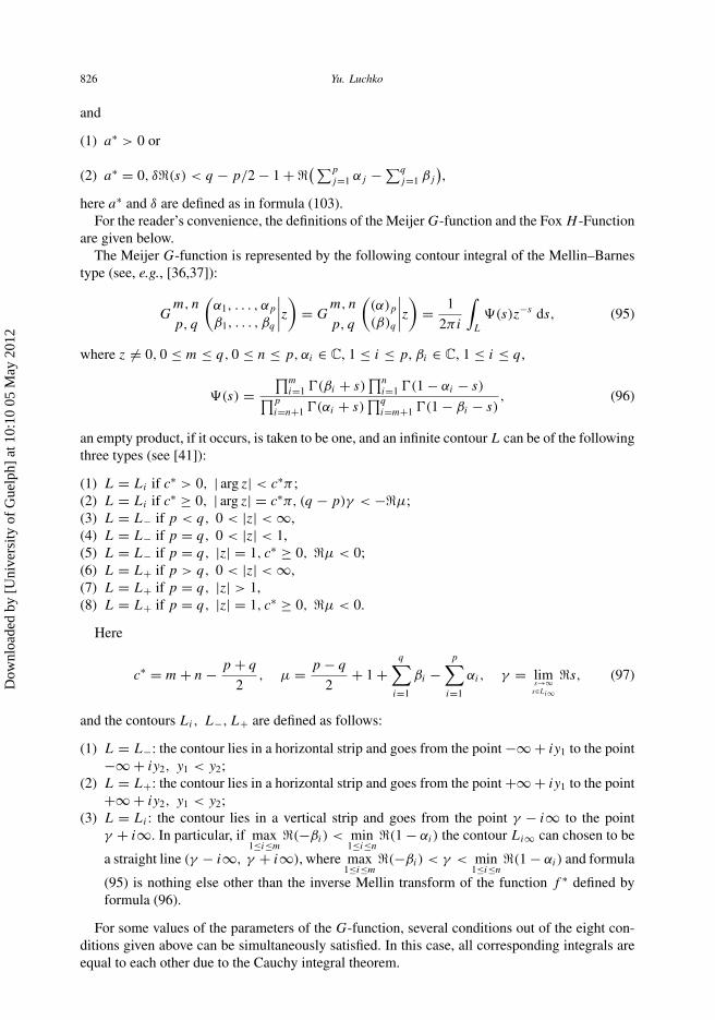
here a∗ and δ are defined as in formula (103).For the reader’s convenience, the definitions of the Meijer G-function and the Fox H -Function
are given below.The Meijer G-function is represented by the following contour integral of the Mellin–Barnes
type (see, e.g., [36,37]):
Gm, n
p, q
(α1, . . . , αp
β1, . . . , βq
∣∣∣∣z) = Gm, n
p, q
((α)p(β)q
∣∣∣∣z) = 1
2πi
∫L
�(s)z−s ds, (95)
where z = 0, 0 ≤ m ≤ q, 0 ≤ n ≤ p, αi ∈ C, 1 ≤ i ≤ p, βi ∈ C, 1 ≤ i ≤ q,
�(s) =∏m
i=1 (βi + s)∏n
i=1 (1 − αi − s)∏p
i=n+1 (αi + s)∏q
i=m+1 (1 − βi − s), (96)
an empty product, if it occurs, is taken to be one, and an infinite contour L can be of the followingthree types (see [41]):
(1) L = Li if c∗ > 0, | arg z| < c∗π ;(2) L = Li if c∗ ≥ 0, | arg z| = c∗π, (q − p)γ < −�μ;(3) L = L− if p < q, 0 < |z| < ∞,(4) L = L− if p = q, 0 < |z| < 1,(5) L = L− if p = q, |z| = 1, c∗ ≥ 0, �μ < 0;(6) L = L+ if p > q, 0 < |z| < ∞,(7) L = L+ if p = q, |z| > 1,(8) L = L+ if p = q, |z| = 1, c∗ ≥ 0, �μ < 0.
Here
c∗ = m + n − p + q
2, μ = p − q
2+ 1 +
q∑i=1
βi −p∑
i=1
αi, γ = lims→∞
s∈Li∞�s, (97)
and the contours Li, L−, L+ are defined as follows:
(1) L = L−: the contour lies in a horizontal strip and goes from the point −∞ + iy1 to the point−∞ + iy2, y1 < y2;
(2) L = L+: the contour lies in a horizontal strip and goes from the point +∞ + iy1 to the point+∞ + iy2, y1 < y2;
(3) L = Li : the contour lies in a vertical strip and goes from the point γ − i∞ to the pointγ + i∞. In particular, if max
1≤i≤m�(−βi) < min
1≤i≤n�(1 − αi) the contour Li∞ can chosen to be
a straight line (γ − i∞, γ + i∞), where max1≤i≤m
�(−βi) < γ < min1≤i≤n
�(1 − αi) and formula
(95) is nothing else other than the inverse Mellin transform of the function f ∗ defined byformula (96).
For some values of the parameters of the G-function, several conditions out of the eight con-ditions given above can be simultaneously satisfied. In this case, all corresponding integrals areequal to each other due to the Cauchy integral theorem.
Dow
nloa
ded
by [
Uni
vers
ity o
f G
uelp
h] a
t 10:
10 0
5 M
ay 2
012
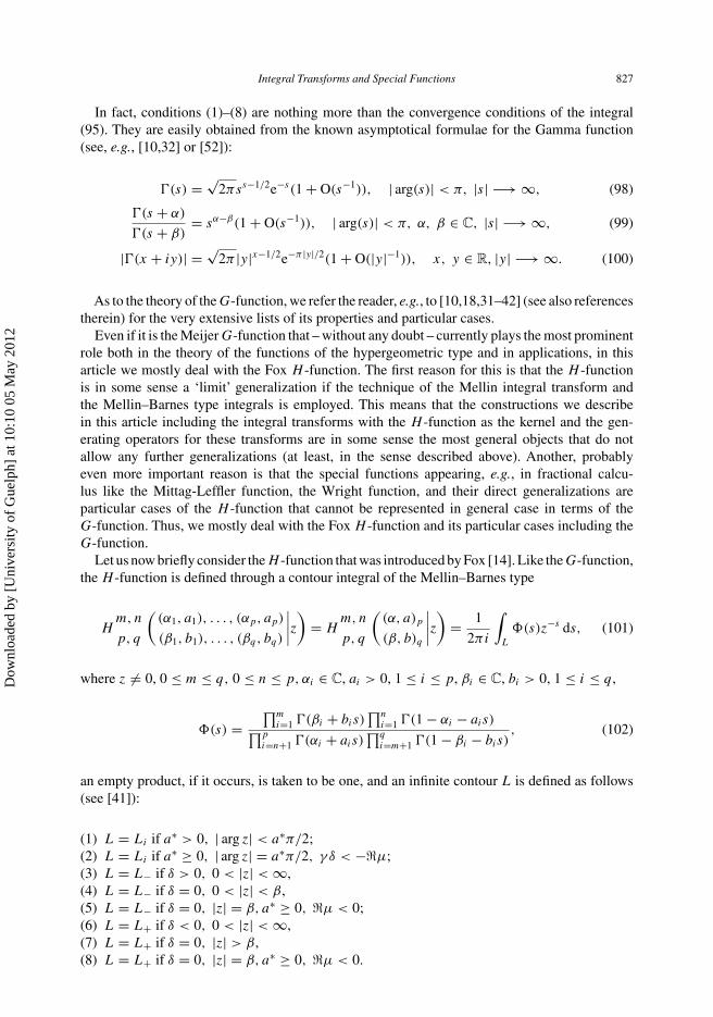
Integral Transforms and Special Functions 827
In fact, conditions (1)–(8) are nothing more than the convergence conditions of the integral(95). They are easily obtained from the known asymptotical formulae for the Gamma function(see, e.g., [10,32] or [52]):
(s) = √2πss−1/2e−s(1 + O(s−1)), | arg(s)| < π, |s| −→ ∞, (98)
(s + α)
(s + β)= sα−β(1 + O(s−1)), | arg(s)| < π, α, β ∈ C, |s| −→ ∞, (99)
|(x + iy)| = √2π |y|x−1/2e−π |y|/2(1 + O(|y|−1)), x, y ∈ R, |y| −→ ∞. (100)
As to the theory of the G-function, we refer the reader, e.g., to [10,18,31–42] (see also referencestherein) for the very extensive lists of its properties and particular cases.
Even if it is the Meijer G-function that – without any doubt – currently plays the most prominentrole both in the theory of the functions of the hypergeometric type and in applications, in thisarticle we mostly deal with the Fox H -function. The first reason for this is that the H -functionis in some sense a ‘limit’ generalization if the technique of the Mellin integral transform andthe Mellin–Barnes type integrals is employed. This means that the constructions we describein this article including the integral transforms with the H -function as the kernel and the gen-erating operators for these transforms are in some sense the most general objects that do notallow any further generalizations (at least, in the sense described above). Another, probablyeven more important reason is that the special functions appearing, e.g., in fractional calcu-lus like the Mittag-Leffler function, the Wright function, and their direct generalizations areparticular cases of the H -function that cannot be represented in general case in terms of theG-function. Thus, we mostly deal with the Fox H -function and its particular cases including theG-function.
Let us now briefly consider theH -function that was introduced by Fox [14]. Like theG-function,the H -function is defined through a contour integral of the Mellin–Barnes type
Hm, n
p, q
((α1, a1), . . . , (αp, ap)
(β1, b1), . . . , (βq, bq)
∣∣∣∣z) = Hm, n
p, q
((α, a)p
(β, b)q
∣∣∣∣z) = 1
2πi
∫L
�(s)z−s ds, (101)
where z = 0, 0 ≤ m ≤ q, 0 ≤ n ≤ p, αi ∈ C, ai > 0, 1 ≤ i ≤ p, βi ∈ C, bi > 0, 1 ≤ i ≤ q,
�(s) =∏m
i=1 (βi + bis)∏n
i=1 (1 − αi − ais)∏p
i=n+1 (αi + ais)∏q
i=m+1 (1 − βi − bis), (102)
an empty product, if it occurs, is taken to be one, and an infinite contour L is defined as follows(see [41]):
(1) L = Li if a∗ > 0, | arg z| < a∗π/2;(2) L = Li if a∗ ≥ 0, | arg z| = a∗π/2, γ δ < −�μ;(3) L = L− if δ > 0, 0 < |z| < ∞,(4) L = L− if δ = 0, 0 < |z| < β,(5) L = L− if δ = 0, |z| = β, a∗ ≥ 0, �μ < 0;(6) L = L+ if δ < 0, 0 < |z| < ∞,(7) L = L+ if δ = 0, |z| > β,(8) L = L+ if δ = 0, |z| = β, a∗ ≥ 0, �μ < 0.
Dow
nloa
ded
by [
Uni
vers
ity o
f G
uelp
h] a
t 10:
10 0
5 M
ay 2
012

828 Yu. Luchko
In conditions (1)–(8), γ and μ are defined as in Equation (97), the values of a∗, δ, β are given by
a∗ =n∑
i=1
ai −p∑
i=n+1
ai +m∑
i=1
bi −q∑
i=m+1
bi, δ =q∑
i=1
bi −p∑
i=1
ai, β =p∏
i=1
a−ai
i
q∏i=1
bbi
i ,
(103)and the contours Li, L−, L+ are taken as in the case of the G-function.
Once again, conditions (1)–(8) are convergence conditions of the integral (101) that followfrom the asymptotical formulae (98) and (100) for the Gamma–function (41).
5. Functional spaces associated with the Mellin integral transform
As we have seen in the previous section, the Mellin transforms of the functions of thehypergeometric type are represented in the form∏m
i=1 (αi + ais)∏n
i=1 (βi − bis)∏li=1 (γi + cis)
∏ki=1 (δi − dis)
, αi, βi, γi, δi ∈ C, ai, bi, ci, di > 0, (104)
i.e., as quotients of products of the Gamma functions with the linear functions of the independentvariable as their arguments. This fact is used throughout the whole article, in one from or another. Inparticular, in this section we describe some special spaces of functions that appear in a very naturalway while studying properties of a large class of the integral transforms of the Mellin convolutiontype with the functions of the hypergeometric type as the kernels. These classes of functionstake into account both the structure of the direct and inverse Mellin integral transforms and theasymptotics of the expression (104) when |�s| → ∞ that easily follows from the asymptotics ofthe Gamma function given by Equations (98)–(100). If the integral transforms with the functionsof the hypergeometric type as the kernels are defined through the right-hand side of the Parsevalequality (65) then a unified theory of such integral transforms can be constructed without takinginto account any specific properties of their kernels. We present some elements of this theory inSection 6.
The idea behind this approach is based on the fact that even if different functions of thehypergeometric type behave differently, their Mellin integral transforms have the same form andsimilar properties. As presented in Sections 6 and 7, these simple considerations let us to developa very general theory of the integral transforms of the Mellin convolution type with the functionsof the hypergeometric type as the kernels and to construct their generating operators.
Following [49,50,52] we first introduce the space M−1(L).
DEFINITION 3 A function f is said to belong to the space M−1(L) if it can be represented as
f (x) = M−1{f ∗(s); x} = 1
2πi
∫σ
f ∗(s) x−s ds, x > 0, σ ={s ∈ C : �(s) = 1
2
}, (105)
where f ∗ ∈ L(σ).
Equipped with the operations of usual addition and multiplication by scalar and with the norm
‖ f ‖M−1(L)= 1
2π
∫ +∞
−∞
∣∣∣∣f ∗(
1
2+ it
)∣∣∣∣ dt, (106)
the space M−1(L) becomes a Banach space.
Dow
nloa
ded
by [
Uni
vers
ity o
f G
uelp
h] a
t 10:
10 0
5 M
ay 2
012
Integral Transforms and Special Functions 829
The features of M−1(L) that are needed in the further discussions can be obtained directlyfrom the definition of the space M−1(L) and from the known properties of the Mellin integraltransform and are collected in the following lemma.
LEMMA 1 Let f ∈ M−1(L). Then
(1) x−1f (x−1) ∈ M−1(L) and vice versa, if x−1f (x−1) ∈ M−1(L) then f ∈ M−1(L).(2) x1/2f (x) is uniformly bounded, continuous on (0, +∞), and the relation x1/2f (x) = o(1)
when x → +∞ and x → 0 holds true.(3) If g ∈ M−1(L) then x1/2f (x)g(x) ∈ M−1(L).
(4) If x−1/2g(x) ∈ L(R+) then fM∗ g ∈ M−1(L).
In the space M−1(L), several useful theorems concerning integral transforms of the Mellinconvolution type can be easily proved for a sufficiently large class of kernels containing, e.g., manyfunctions of the hypergeometric type. This class of kernels is introduced in the following definition.
DEFINITION 4 ([49]) A function k : (0, ∞) → R is said to belong to the class K of kernels if itsatisfies the following conditions:
(1) k ∈ L(ε, E) for any ε, E such that 0 < ε < E < ∞.(2) The integral
k∗(s) = M{k(u); s} =∫ ∞
0k(u)us−1du, s ∈ σ, σ =
{s ∈ C : �(s) = 1
2
}(107)
converges for any s ∈ σ .(3) For almost all ε, E > 0 and t ∈ R∣∣∣∣ ∫ E
ε
k(u)uit−1/2du
∣∣∣∣ < Ck, (108)
where the constant Ck > 0 does not depend on ε, E, and t .If for a function k ∈ K there exists a kernel k∗ ∈ K such that the equality
k∗(s)k∗(1 − s) = 1, k, k ∈ K (109)
holds true almost everywhere on the line �(s) = 1/2, we say that k ∈ K∗ ⊂ K. The kernelk ∈ K∗ satisfying Equation (109) is called a conjugate kernel of the kernel k ∈ K∗ (and viceversa, the kernel k is conjugate of k).
It is easy to check that if x−1/2k(x) ∈ L(0, ∞), then k ∈ K but k ∈ K∗.Following [25,26,48,49,52] we consider in this part of the section the integral transforms of
the Mellin convolution type
g(x) = (Kf )(x) =∫ ∞
0k(xy)f (y) dy (110)
with the kernels from the space K and their inverse transforms
f (x) = (Kg)(x) =∫ ∞
0k(xy)g(y) dy (111)
with the kernels from the space K∗ and some of their properties in the functional space M−1(L).The main results we use in the further discussions are formulated in Theorems 3 and 4 (for theproofs we refer the interested reader to [48,49,52]).
Dow
nloa
ded
by [
Uni
vers
ity o
f G
uelp
h] a
t 10:
10 0
5 M
ay 2
012

830 Yu. Luchko
THEOREM 3 ([48]) Let f ∈ M−1(L), k ∈ K, k∗ be given by Equation (107) and f ∗ be definedas in Equation (105). Then the Parseval formula∫ ∞
0k(xy)f (y) dy = 1
2πi
∫σ
k∗(s)f ∗(1 − s)x−s ds (112)
holds true.
THEOREM 4 Let k ∈ K∗ and k ∈ K∗ be its conjugate kernel. Then the integral transform
g(x) = (Kf )(x) =∫ ∞
0k(xy)f (y) dy
is an automorphism in the space M−1(L) and its inverse transform is given by
f (x) = (Kg)(x) =∫ ∞
0k(xy)g(y) dy.
COROLLARY 1 Let k ∈ K∗, k ∈ K∗ be its conjugate kernel, and |k∗(s)| = 1, s ∈ σ . Then theintegral transforms (110) and (111) are isometric automorphisms in the space M−1(L).
Example 5 The sine-Fourier transform
(Fsf )(x) =√
2
π
∫ ∞
0sin(xy)f (y) dy (113)
is an isometric automorphism in the space M−1(L) and its inverse transform has the same form.
Example 6 The modified Hankel transform
(Jνf )(x) =∫ ∞
0Jν(2
√xy)f (y) dy, �(ν) > −1 (114)
is an automorphism in the space M−1(L) and its inverse transform has the same form. If ν ∈ R,then the modified Hankel transform (114) is an isometric automorphism in the space M−1(L).
These examples are particular cases of the following important theorem.
THEOREM 5 ([49,52]) Let the conditions
q − m − n = m + n − p = η
2= 0, (115)
�⎛⎝ p∑
j=1
αj −q∑
j=1
βj
⎞⎠ = 0, (116)
�(αj ) <1
2, 1 ≤ j ≤ n; �(βj ) > −1
2, 1 ≤ j ≤ m; (117)
�(αj ) > −1
2, n + 1 ≤ j ≤ p; �(βj ) <
1
2, m + 1 ≤ j ≤ q. (118)
hold true. Then the kernel defined in terms of the Meijer G-function in the form
k(x) = Gm,np,q
((α)p(β)q
∣∣∣∣x) (119)
Dow
nloa
ded
by [
Uni
vers
ity o
f G
uelp
h] a
t 10:
10 0
5 M
ay 2
012

Integral Transforms and Special Functions 831
belongs to the class K∗ of kernels and its conjugate kernel is given by
k(x) = Gq−m,p−np,q
(−(α)p
n+1, −(α)n1−(β)q
m+1, −(β)m1
∣∣∣∣x) , (120)
where the symbol (a)j
i denotes the set {ai, ai+1, ai+2, . . . , aj }.
As known in the theory of special functions, the Fox H -function is a very general object thathas the Meijer G-function among its particular cases. Following [25,26], a Mellin convolutiontype transform with a particular case of the H -function as the kernel is considered in this part ofthe section. Because this kernel can also be written in terms of the G-function, we prefer to giveall formulations by using the ‘language’ of the G-function.
DEFINITION 5 ([25,26]) Let β, η > 0, m ∈ N, γj ∈ R, j = 1, . . . , 2m. The integral transformof the Mellin convolution type
g(x) = (Hβf )(x) =∫ ∞
0Hβ(xy) f (y) dy, x > 0, (121)
with the kernel
Hβ(x) = β√ηG
m,00,2m
(−
(γj + 1 − 1β)2m
∣∣∣∣ (x
η
)β)
(122)
is called the generalized Hankel integral transform.
The classical Hankel integral transform
(Jνf )(x) =∫ ∞
0
√xy Jν(xy)f (y) dy (123)
is a particular case of the generalized Hankel integral transform (121) with β = 2, η = 2, m =2, γ1 = −1/4 + ν/2, γ2 = −1/4 − ν/2. Another more important reason to call the transform(121) the generalized Hankel transform is that this integral transform plays the same role forthe hyper-Bessel differential operator as the Hankel transform does for the Bessel differentialoperator, i.e., the hyper-Bessel differential operator is the generating operator of the generalizedHankel transform. These results are presented in Section 7.
THEOREM 6 ([25,26]) The generalized Hankel integral transform (121) is an automorphism inthe space M−1(L) under the conditions
m +2m∑j=1
γj = m
β; γj >
1
2β− 1, j = 1, . . . , m; γj <
1
2β, j = m + 1, . . . , 2m, (124)
and its inverse transform is given by
f (x) = (Hβg)(x) =∫ ∞
0Hβ(xt)g(t) dt, x > 0, (125)
where
Hβ(x) = β√ηG
m,00,2m
(−
(−γj )2mm+1, (−γj )
m1
∣∣∣∣ (x
η
)β)
.
Dow
nloa
ded
by [
Uni
vers
ity o
f G
uelp
h] a
t 10:
10 0
5 M
ay 2
012

832 Yu. Luchko
Probably the most interesting case of a pair of the integral transforms (110), (111) is thesymmetrical one, i.e., the case when both transforms have the same form. For the generalizedHankel integral transform (121) this situation takes place if and only if γj + γj+m = 1/β − 1, j =1, . . . , m. Then Theorem 6 can be rewritten as follows.
THEOREM 7 ([25,26]) Under the conditions
γj >1
2β− 1, j = 1, . . . , m,
the generalized symmetrical Hankel integral transform
g(x) = (Gβf )(x) =∫ ∞
0Gβ(xy)f (y) dy, x > 0, (126)
where
Gβ(x) = β√ηG
m,00,2m
(−
(γj + 1 − 1β)m, (−γj )m
∣∣∣∣ (x
η
)β)
, β, η > 0
is an isometric automorphism in the space M−1(L) and its inverse transform has the same form.
A result similar to the statement of Theorem 7 can be proved for the direct and inverse integraltransforms from Theorem 5, too. In general, the kernels (119) and (120) do not match like thekernels of the generalized Hankel integral transform and its inverse transform. The case of thesymmetrical transforms, i.e., the case when the kernel (119) coincides with the conjugate kernel(120) is described in the following theorem.
THEOREM 8 ([49]) Let the conditions
m = n, αj <1
2, 1 ≤ j ≤ n, βj > −1
2, 1 ≤ j ≤ m (127)
hold true. Then the integral transform
g(x) =∫ ∞
0G
m,n2n,2m
((α)n, −(α)n
(β)m, −(β)m
∣∣∣∣xy
)f (y) dy (128)
is an isometric automorphism in the space M−1(L) and its inverse transform has the same form.
As we have seen in this section, the Mellin convolution type integral transforms defined as
g(x) = (Kf )(x) =∫ ∞
0k(xy)f (y) dy
with the kernels from the space K∗ as well as their inverse transforms can be very easily describedand investigated in the functional space M−1(L). This fact becomes clear if we note that thespace M−1(L) is defined in terms of the inverse Mellin integral transform, i.e., the class of theintegral transforms and the functional space they act in are well adjusted each to other.
Even if the class K∗ of kernels contains some important special functions of the hypergeometrictype (see the examples and theorems given earlier in this section) it is not large enough to includethe G- and H -functions in the general case. The reason for this situation is in the asymptoticsof the Mellin integral transforms of the G- and H -functions that are given by formulae (93) and(94), respectively. As we have seen in Section 3, the Mellin transforms of the functions of the
Dow
nloa
ded
by [
Uni
vers
ity o
f G
uelp
h] a
t 10:
10 0
5 M
ay 2
012

Integral Transforms and Special Functions 833
hypergeometric type are given by quotients of the products of the Gamma functions (104). Whens ∈ σ(�(s) = 1/2), the asymptotics of the expression (104) is as follows:
f ∗(s) = |s|−γ e−πc|�(s)|(C + O(|s|−1), |�(s)| → ∞, (129)
where C is a constant,
γ = 1
2(m + n − k − l) −
m∑i=1
(αi + 1
2ai
)−
n∑i=1
(βi − 1
2bi
)+
l∑i=1
(γi + 1
2ci
)
+k∑
i=1
(δi − 1
2di
), (130)
c = 1
2
(n∑
i=1
ai +m∑
i=1
bi −l∑
i=1
ci −k∑
i=1
di
). (131)
Formula (129) is a simple consequence of formula (100) that gives the asymptotics of theGamma function.
In particular, it follows from the asymptotics (129) and the Mellin transform formula (93) forthe G-function that conditions (115)–(118) of Theorem 5 mean, among other things, that boththe Mellin transform k∗ of the G-function (119) considered in the theorem and the expression1/k∗(1 − s) are restricted when �(s) → ∞. This special asymptotics ensures that the G-function(119) belongs to the class K∗ of the kernels. If conditions (115)–(118) are not satisfied, i.e., if theMellin transform of the G-function or of another function of the hypergeometric type is allowedto grow or to decrease when �(s) → ∞ then we need to take their asymptotics into considerationwhile defining the functional spaces where the Mellin convolution type integral transforms withthe hypergeometric type functions as the kernels act in.
In the remainder of this section, we introduce such functional spaces that are used in Sections 6and 7 while discussing the H -transform, the generalized H -transform and their generating oper-ators. The H -transform is nothing else than the integral transform of the Mellin convolution typewith the Fox H -function as the kernel. The asymptotics of the Mellin transform of the H -functionis given by an expression of the type (129). The asymptotics (129) play the role of a weightfunction in the definition of the space M−1
c,γ (L). This space is in fact a special subspace of thespace M−1(L), which takes into consideration the asymptotics of the Mellin transform of theH -function and its analytical properties.
DEFINITION 6 A function f is said to belong to the space M−1c,γ (L) if it can be represented in the
form
f (x) = M−1{f ∗(s); x} = 1
2πi
∫σ
f ∗(s) x−s ds, x > 0, σ ={s ∈ C : �(s) = 1
2
}(132)
with a function f ∗ such that
f ∗(s)|s|γ eπc|�(s)| ∈ L(σ), (133)
and
2 sgn(c) + sgn(γ ) ≥ 0, c, γ ∈ R. (134)
Because |�(s)| ≈ |s| when |s| → ∞, s ∈ σ , the integral (132) converges if c > 0, γ ∈ R orif c = 0, γ ≥ 0, i.e., under the condition (134).
Dow
nloa
ded
by [
Uni
vers
ity o
f G
uelp
h] a
t 10:
10 0
5 M
ay 2
012

834 Yu. Luchko
The space M−1c,γ (L) is a Banach space with the norm
‖f ‖M−1c,γ (L) = 1
2π
∫σ
eπc|�(s)||sγ f ∗(s) ds|. (135)
If c = 0, γ = 0, the space M−1c,γ (L) coincides with the whole space M−1(L). In the general
situation, the inclusion
M−1c1,γ1
(L) ⊂ M−1c,γ (L) (136)
holds true if and only if
2 sgn(c1 − c) + sgn(γ1 − γ ) ≥ 0. (137)
Another important subspace of the space M−1(L) has been introduced and investigated by theauthor in [23] (see also [52]). This space plays an important role while considering the generatingoperators of the generalized H -transform (see Section 7).
DEFINITION 7 Let c, λ ≥ 0, γ ∈ R and the condition
2 sgn(c) + sgn(γ ) ≥ 0 (138)
hold true. By λM−1c,γ we denote the space of all functions that can be represented in the form
f (x) = 1
2πi
∫σ(1/2)
f ∗(s)x−s ds, x > 0, σ (τ ) = {s ∈ C : �(s) = τ } (139)
with a function f ∗, analytical in the strip |�(s) − 1/2| ≤ λ, such that f ∗(s) = |1/2 +i�(s)|−γ e−πc|�(s)|F(s), where the function F satisfies the following conditions:∫
σ(τ)
|F(s) ds| ≤ CF for
∣∣∣∣τ − 1
2
∣∣∣∣ ≤ λ, (140)
with a constant CF not depending on λ,
F(s) → 0 when �(s) → ∞ (141)
uniformly with respect to �(s) in the strip |�(s) − 1/2| ≤ λ.
It is clear that the space λM−1c,γ is a subspace of the space M−1
c,γ (L) introduced earlier in thissection. Of course, the set of spaces λM−1
c,γ can be partially ordered:
λ1M−1c1,γ1
⊆ λM−1c,γ
if
λ1 ≥ λ, 2 sgn(c1 − c) + sgn(γ1 − γ ) ≥ 0. (142)
One of the important properties of the space λM−1c,γ is given by the following theorem.
THEOREM 9 Let ρ ∈ R, λ > 0, |ρ| ≤ λ. If f ∈ λM−1c,γ then the function xρf (x) belongs to the
space λ1M−1c,γ , where λ1 = min{λ − ρ, λ + ρ} and
xρf (x) = 1
2πi
∫σ( 1
2 )
f ∗(s + ρ)x−s ds, x > 0. (143)
Dow
nloa
ded
by [
Uni
vers
ity o
f G
uelp
h] a
t 10:
10 0
5 M
ay 2
012

Integral Transforms and Special Functions 835
The proof of the theorem can be found in [23,52].Let us mention that a functional space similar to the space λM−1
c,γ has been introduced earlierand studied in [3]. The result proved in Theorem 9 is especially important while consideringthe generating operators of the generalized H -transform in Section 7. Indeed, the generatingoperator of the generalized H -transform translates the action of the generalized H -transform intooperation of multiplication by a power function. To study the mapping properties of the generatingoperator of the generalized H -transform, we thus need to trace the action of the operation ofmultiplication by a power function that is described by Theorem 9.
6. H-transform and the generalized H-transform
In this section, we consider the Mellin convolution-type transform (110) with Fox’s H -function(101) as the kernel in the space M−1
c,γ (L). For the theory of this transform in other functionalspaces see the recent book [19] and references therein.
The H -transform is defined by
[Hf ](x) = g(x) =∫ ∞
0Hm,n
p,q
((αp, ap)
(βq, bq)
∣∣∣∣xu
)f (u) du, (144)
where the Fox H -function Hm,np,q is given by Equation (101). The inversion of the H -transform
in the space M−1c,γ (L) and its other properties have been studied in [23] (see also [52]). In par-
ticular, we refer to the following important theorem that describes the mapping properties of theH -transform and its inversion formula.
THEOREM 10 Let f (x) ∈ M−1c,γ (L) and
�(βj ) + bj
2> 0, 1 ≤ j ≤ m; 1 − �(αj ) − aj
2> 0, 1 ≤ j ≤ n, (145)
2 sgn(κ) + sgn(μ − 1) > 0, (146)
2 sgn(c + κ) + sgn(γ + μ) ≥ 0, (147)
where
κ = 1
2
⎛⎝ m∑j=1
bj +n∑
j=1
aj −p∑
j=n+1
aj −q∑
j=m+1
bj
⎞⎠, (148)
μ = �⎛⎝ p∑
j=1
αj −q∑
j=1
βj
⎞⎠+ 1
2
⎛⎝ p∑j=1
aj −q∑
j=1
bj
⎞⎠− p − q
2. (149)
Then the H -transform (144) exists and the following inclusion holds true:
g(x) = [Hf ](x) ∈ M−1c+κ,γ+μ(L). (150)
If, in addition,
�(αj ) + aj
2> 0, n + 1 ≤ j ≤ p; 1 − �(βj ) − bj
2> 0, m + 1 ≤ j ≤ q, (151)
then the H -transform is the one-to-one correspondence from the space M−1c,γ (L) onto the space
M−1c+κ,γ+μ(L) and its inverse has the following form:
Dow
nloa
ded
by [
Uni
vers
ity o
f G
uelp
h] a
t 10:
10 0
5 M
ay 2
012

836 Yu. Luchko
(a) In the case κ = 0, μ > 1
f (x) = [Hg](x) = dk
dxkxk
∫ ∞
0H
q−m,p−n+1p+1,q+1
((αp+1, ap+1)
(βq+1, bq+1)
∣∣∣∣xu
)g(u) du, (152)
where k ∈ N, k > μ + 1, (αp+1, ap+1) = {(0, 1), (1 − αi − ai, ai)p
n+1, (1 − αi − ai, ai)n1},
(βq+1, bq+1) = {(1 − βi − bi, bi)q
m+1, (1 − βi − bi, bi)m1 , (−k, 1)}.
(b) In the case κ > 0
f (x) = [Hg](x) = limk→∞
kk
(k − 1)!xk/r
(rx(r+1)/r d
dx
)k
×∫ ∞
0H
q−m+1,p−n
p,q+1
((αp, ap)
(βq+1, bq+1)
∣∣∣∣krxu
)g(u) du, (153)
where r ∈ N, r > 2κ, (αp, ap) = {(1 − αi − ai, ai)p
n+1, (1 − αi − ai, ai)n1}, (βq+1, bq+1) =
{(0, r), (1 − βi − bi, bi)q
m+1, (1 − βi − bi, bi)m1 }.
Now we consider some examples of the H -transform and, in particular, the Erdélyi-Koberfractional integration operators.
Example 7 The Erdélyi–Kober fractional integration operators have the form ([20,21,45,52])
[I γ,δ
β f ](x) = β
(δ)x−β(γ+δ)
∫ x
0(xβ − uβ)δ−1uβ(γ+1)−1f (u) du, (154)
[Kτ,αβ f ](x) = β
(α)xβτ
∫ ∞
x
(uβ − xβ)α−1u−β(τ+α−1)−1f (u) du, (155)
where β > 0, �(δ) > 0, �(α) > 0. For δ = 0 or α = 0, respectively, these operators are definedas the identity operator:
[I γ,0β f ] ≡ Id, [Kτ,0
β f ](x) ≡ Id.
The Erdélyi–Kober fractional integration operators (154), (155) are reduced to the Riemann–Liouville fractional integration operators with the power weights in the case β = 1:
(x−γ−δI δ0+xγ f )(x) = 1
(δ)x−γ−δ
∫ x
0(x − u)δ−1uγ f (u) du, (156)
(xτ I α−x−τ−αf )(x) = 1
(α)xτ
∫ ∞
x
(u − x)α−1u−τ−αf (u) du. (157)
Using the relations (73), (74), formulae (154) and (155) can be represented in the form
[I γ,δ
β f ](x) =∫ ∞
0H1(xu)f (u−1)
du
u, (158)
where H1(u) = H0,11,1
((−γ,1/β)
(−γ−δ,1/β)
∣∣u) ,
[Kτ,αβ f ](x) =
∫ ∞
0H2(xu)f (u−1)
du
u, (159)
where H2(u) = H1,01,1
((τ+α,1/β)
(τ,1/β)
∣∣u) . According to Lemma 1, f (u) ∈ M−1c,γ (L) iff f (u−1)u−1 ∈
M−1c,γ (L). Thus we can apply Theorem 10 to the transforms (158), (159) and obtain the existence
Dow
nloa
ded
by [
Uni
vers
ity o
f G
uelp
h] a
t 10:
10 0
5 M
ay 2
012

Integral Transforms and Special Functions 837
condition
1 + �(γ ) >1
2β, �(δ) > 1 (160)
for the transform (158) on the space M−1c,γ (L) as well as the inclusion g(x) = [I γ,δ
β f ](x) ∈M−1
c,γ+�(δ)(L). The condition �(δ) > 1 is a very restrictive one. It can be replaced by the condition�(δ) > 0 by observing the following relation for the kernel of the transform (158):
H1(u) = H0,11,1
((−γ, 1/β)
(−γ − δ, 1/β)
∣∣∣∣u) = βG0,11,1
( −γ
−γ − δ
∣∣∣∣uβ
), (161)
that permits the results for the G-transform to apply (see, e.g., [52]) to the transform (158) suchthat we obtain the same existence statement under the weaker condition �(δ) > 0.
Since M{f (u−1)u−1; s} = f ∗(1 − s), the Parseval formula (65) has the form
g(x) = [I γ,δ
β f ](x) = 1
2πi
∫σ
k∗(s)f ∗(s)x−s ds, (162)
where k∗(s) = (1 + γ − s/β)/(1 + γ + δ − s/β). It follows from Theorem 10 that the trans-form (158) is a one-to-one correspondence from the space M−1
c,γ (L) onto the space M−1c,γ+�(δ)(L).
Theorem 10 could be now applied to obtain the inversion for the Erdélyi–Kober fractional integral(158), but we prefer to use a slightly different approach. From the relation (162) we obtain
f ∗(s) = (1 + γ + δ − s/β)
(1 + γ − s/β)g∗(s) = (1 + γ + δ − s/β)
(1 + γ + η − s/β)
(1 + γ − s
β
)η
g∗(s), (163)
where
η ={
[�(δ)] + 1, δ ∈ Z,
δ, δ ∈ Z.
Since the function
H3(u) = H0,11,1
((−γ − δ, 1/β)
(−γ − η, 1/β)
∣∣∣∣u) (164)
has the same properties as the function H1 defined by (161), we can apply the Parseval formula(65), the relation (70) and thus obtain the inversion formula:
η∏j=1
(γ + j + 1
βx
d
dx
)[I γ+δ,η−δ
β g](x) =η∏
j=1
(γ + j + 1
βx
d
dx
)∫ ∞
0H3(xu)g(u−1)
du
u
= 1
2πi
η∏j=1
(γ + j + 1
βx
d
dx
)∫σ
(1 + γ + δ − s/β)
(1 + γ + η − s/β)g∗(s)x−s ds
= 1
2πi
∫σ
(1 + γ + δ − s/β)
(1 + γ + η − s/β)(1 + γ − s/β)η
(1 + γ − s/β)
(1 + γ + δ − s/β)f ∗(s)x−s ds
= 1
2πi
∫σ
f ∗(s)x−s ds = f (x). (165)
The operator
[Dγ,δ
β g](x) ≡η∏
j=1
(γ + j + 1
βx
d
dx
)[I γ+δ,η−δ
β g](x), (166)
where η is determined by the relation (163) is called the Erdélyi–Kober fractional derivative.
Dow
nloa
ded
by [
Uni
vers
ity o
f G
uelp
h] a
t 10:
10 0
5 M
ay 2
012

838 Yu. Luchko
For the Erdélyi–Kober fractional integral (155), the same considerations can be used to showthat this transform is a one-to-one correspondence from the space M−1
c,γ (L) onto the space
M−1c,γ+�(α)(L) under the conditions
�(τ ) + 1
2β> 0, �(α) > 0 (167)
and the inverse transform (the Erdélyi–Kober fractional derivative) is given by the formula
f (x) =η−1∏j=0
(τ + j − 1
βx
d
dx
)[Kτ+α,η−α
β g](x) = [P τ,αβ g](x), (168)
where
η ={
[�(α)] + 1, α ∈ Z,
α, α ∈ Z.
Example 8 Let us consider now a generalization of the Obrechkoff transform ([5,52]) in theform
[Of ](x) = g(x) =∫ ∞
0H
0,nn,0
((α, a)1,n
−∣∣∣∣xu)
f (u)du
u. (169)
By using the definition of the H -function (101) and formula (41), this transform can be representedin the form
[Of ](x) =∫ ∞
0�n
((αi, ai)
n1 | x
u
)f (u)
du
u, (170)
where
�n((αi, ai)n1|τ) = τ (αn−1)/an
an
∫ ∞
0. . .
∫ ∞
0exp
{−
n−1∑i=1
ui − τ−1/an
n−1∏i=1
u−ai/an
i
}
×n−1∏i=1
u−ai (1−αn)/an−αi
i du1 . . . dun−1.
It follows from Theorem 10, that the generalized Obrechkoff transform (169) is a one-to-onemapping from the space M−1
c,γ (L) onto the space M−1c+κ,γ+μ(L) under the conditions
1 − �(αj ) − aj
2> 0, 1 ≤ j ≤ n;
2 sgn(κ) + sgn(μ − 1) > 0;2 sgn(c + κ) + sgn(γ + μ) ≥ 0, (171)
where
κ = 1
2
n∑j=1
aj , μ = �⎛⎝ n∑
j=1
αj
⎞⎠+ 1
2
n∑j=1
aj − n
2.
The Parseval formula (65) for the generalized Obrechkoff transform takes the form
[Of ](x) = g(x) = 1
2πi
∫σ
n∏j=1
(1 − αj − aj s)f∗(s)x−s ds. (172)
Dow
nloa
ded
by [
Uni
vers
ity o
f G
uelp
h] a
t 10:
10 0
5 M
ay 2
012

Integral Transforms and Special Functions 839
The relation (172) leads to the representation
f ∗(s) = g∗(s)∏nj=1 (1 − αj − aj s)
. (173)
To obtain the real inversion formula for the generalized Obrechkoff transform, the same consid-erations as for the Laplace transform (see, e.g., [51]) can be used. The result is as follows [52]):
f (x) = limk1,...,kn→∞
n∏j=1
kαj −1j
kj !kj −1∏i=0
(i + 1 − αj + ajx
d
dx
)g
⎛⎝x
n∏j=1
kj
⎞⎠. (174)
Example 9 Following the author’s paper [25], we consider now the generalized Obrechkoff–Stieltjes transform. The generalized Obrechkoff transform has been already introduced in theprevious example, so let us define the generalized Stieltjes transform ([24,52]):
[Sαβ f ](x) = xα/β
β
∫ ∞
0
f (u)u(1−α)/β
x1/β + u1/β
du
u, u > 0, β > 0. (175)
The case α = 0, β = 1 of the operator (175) corresponds to the classical Stieltjes transform.The Parseval formula (65) and formulae (67), (68), and (75) lead to the following representation
of the generalized Stieltjes transform (175) on the space M−1(L):
[Sαβ f ](x) = 1
2πi
∫σ
(1 − α − βs)(α + βs)f ∗(s)x−s ds. (176)
Based on the representations (172) and (176) of the generalized Obrechkoff and Stieltjes trans-forms, let us introduce the generalized Obrechkoff-Stieltjes transform that satisfies the followingrelation:
[OSf ](x) = 1
2πi
∫σ
n∏j=1
(1 − αj − aj s)
m∏j=1
(βj + bj s)f∗(s)x−s ds. (177)
DEFINITION 8 The generalized Obrechkoff–Stieltjes transform is an integral transform of theMellin convolution type with the Fox H -function of a special type as the kernel:
[OSf ](x) =∫ ∞
0Hm,n
n,m
((α, a)1,n
(β, b)1,m
∣∣∣∣xu)
f (u)du
u, u > 0, (178)
where
Hm,nn,m
((α, a)1,n
(β, b)1,m
∣∣∣∣t) = 1
2πi
∫L
�(s)t−s ds,
�(s) =n∏
j=1
(1 − αj − aj s)
m∏j=1
(βj + bj s).
Formula (94) for the Mellin transform of the H -function, the Parseval formula for theMellin integral transform and the asymptotic of the H -function (see, e.g., [19,35,41,52])ensure the representation (177) of the generalized Obrechkoff–Stieltjes transform (178) on thespace M−1(L).
Dow
nloa
ded
by [
Uni
vers
ity o
f G
uelp
h] a
t 10:
10 0
5 M
ay 2
012

840 Yu. Luchko
It follows from the relations (178), (172), and (176) that both the generalized Obrechkoff trans-form and the generalized Stieltjes transform are particular cases of the generalized Obrechkoff–Stieltjes transform (178). Formulae (80)–(87) lead to other particular cases different from theones mentioned above (for the sake of reader’s convenience some constant factors in the kernelsof the integral transforms are omitted in several cases (see formulae (80)–(87)):
(a) modified Meijer’s transform (m = 2, n = 0, b1 = b2 = 1, β1 = ν/2, β2 = −ν/2):
[OSf ](x) =∫ ∞
0Kν
(2
√x
u
)f (u)
du
u, u > 0, (179)
(b) integral transform with the Macdonald function as the kernel (m = 2, n = 1, b1 = b2 = a1 =1, β1 = ν, β2 = −ν, α1 = 1/2):
[OSf ](x) =∫ ∞
0ex/2uKν
( x
2u
)f (u)
du
u, u > 0, (180)
(c) integral transform with the probability integral as the kernel (m = 2,n = 1,b1 = b2 = a1 = 1,β1 = 1/2, β2 = 0, α1 = 1/2):
[OSf ](x) =∫ ∞
0ex/uerfc
(√x
u
)f (u)
du
u, u > 0, (181)
(d) integral transform with the Tricomi function as the kernel (m = 2, n = 1, b1 = b2 = a1 = 1,β1 = 0, β2 = 1 − b, α1 = 1 − a):
[OSf ](x) =∫ ∞
0�(a; b; x
u
)f (u)
du
u, u > 0, (182)
(e) integral transform with the Legendre function of the first kind as the kernel (m = 2, n = 2,b1 = b2 = a1 = a2 = 1, β1 = 0, β2 = 1/2, α1 = 1 − (1 + ν − μ)/2, α2 = 1 + (ν + μ)/2):
[OSf ](x) =∫ ∞
0
∣∣∣1 − x
u
∣∣∣μ/2P μ
ν
(√x
u
)f (u)
du
u, u > 0, (183)
(f) integral transform with the sum of squares of the Bessel function and the Neumann functionas the kernel (m = 3, n = 1, b1 = b2 = b3 = a1 = 1, β1 = 0, β2 = ν, β3 = −ν, α1 = 1/2):
[OSf ](x) =∫ ∞
0
(J 2
ν
(√x
u
)+ Y 2
ν
(√x
u
))f (u)
du
u, u > 0. (184)
Like the Obrechkoff transform (169) the generalized Obrechkoff–Stieltjes transform can berepresented through a multiple integral with an exponential function and power multipliers as thekernel. The corresponding formula can be found in [24].
As we have seen, the inversion formulae for the H -transform and its particular cases dependson the values of κ and μ (see the Theorem 10) which are determined by the parameters of theH -function from the kernel of the H -transform. This fact does not cause much trouble if weconsider a particular case of the H -transform. However, while developing a general theory of theH -transform, a new approach, which unites the already studied cases (κ = 0, μ > 1 and κ > 0)with the new ones (κ = 0, μ ≤ 1 and κ < 0) is needed. This approach is based on the Parsevalformula (65) and was studied in [45,48–50,52]. The main role in this theory is played by thenotion of the generalized H -transform:
Dow
nloa
ded
by [
Uni
vers
ity o
f G
uelp
h] a
t 10:
10 0
5 M
ay 2
012
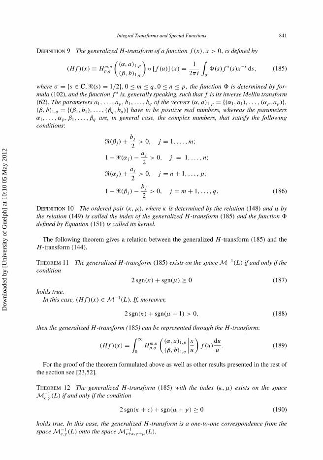
Integral Transforms and Special Functions 841
DEFINITION 9 The generalized H -transform of a function f (x), x > 0, is defined by
(Hf )(x) ≡ Hm,np,q
((α, a)1,p
(β, b)1,q
)◦ [f (u)] (x) = 1
2πi
∫σ
�(s)f ∗(s)x−s ds, (185)
where σ = {s ∈ C, �(s) = 1/2}, 0 ≤ m ≤ q, 0 ≤ n ≤ p, the function � is determined by for-mula (102), and the function f ∗ is, generally speaking, such that f is its inverse Mellin transform(62). The parameters a1, . . . , ap, b1, . . . , bq of the vectors (α, a)1,p = {(α1, a1), . . . , (αp, ap)},(β, b)1,q = {(β1, b1), . . . , (βq, bq)} have to be positive real numbers, whereas the parametersα1, . . . , αp, β1, . . . , βq are, in general case, the complex numbers, that satisfy the followingconditions:
�(βj ) + bj
2> 0, j = 1, . . . , m;
1 − �(αj ) − aj
2> 0, j = 1, . . . , n;
�(αj ) + aj
2> 0, j = n + 1, . . . , p;
1 − �(βj ) − bj
2> 0, j = m + 1, . . . , q. (186)
DEFINITION 10 The ordered pair (κ, μ), where κ is determined by the relation (148) and μ bythe relation (149) is called the index of the generalized H -transform (185) and the function �
defined by Equation (151) is called its kernel.
The following theorem gives a relation between the generalized H -transform (185) and theH -transform (144).
THEOREM 11 The generalized H -transform (185) exists on the space M−1(L) if and only if thecondition
2 sgn(κ) + sgn(μ) ≥ 0 (187)
holds true.In this case, (Hf )(x) ∈ M−1(L). If, moreover,
2 sgn(κ) + sgn(μ − 1) > 0, (188)
then the generalized H -transform (185) can be represented through the H -transform:
(Hf )(x) =∫ ∞
0Hm,n
p,q
((α, a)1,p
(β, b)1,q
∣∣∣∣xu)
f (u)du
u. (189)
For the proof of the theorem formulated above as well as other results presented in the rest ofthe section see [23,52].
THEOREM 12 The generalized H -transform (185) with the index (κ, μ) exists on the spaceM−1
c,γ (L) if and only if the condition
2 sgn(κ + c) + sgn(μ + γ ) ≥ 0 (190)
holds true. In this case, the generalized H -transform is a one-to-one correspondence from thespace M−1
c,γ (L) onto the space M−1c+κ,γ+μ(L).
Dow
nloa
ded
by [
Uni
vers
ity o
f G
uelp
h] a
t 10:
10 0
5 M
ay 2
012

842 Yu. Luchko
THEOREM 13 Let the condition (190) be fulfilled. Then the generalized H -transform[Hm,n
p,q
((α, a)1,p
(β, b)1,q
)]−1
◦ [g(u)] (x) = Hp−n,q−mq,p
((β, b)
q
m+1, (β, b)m1
(α, a)p
n+1, (α, a)n1
)◦ [g(u)] (x)
= 1
2πi
∫σ
1
�(s)g∗(s)x−sds (191)
is the inverse transform of the generalized H -transform (185) in the space M−1c+κ,γ+μ(L).
THEOREM 14 Let
(H1f )(x) ≡ Hm,np,q
((α, a)1,p
(β, b)1,q
)◦ [f (y)] (x), (192)
(H2f )(x) ≡ Hu,vl,t
((ν, c)1,l
(δ, d)1,t
)◦ [f (y)] (x) (193)
be two generalized H -transforms with the indices (κ1, μ1) and (κ2, μ2), respectively. Then thecomposition of these H -transforms
(H2 ◦ H1)(f )(x) = [H2 ◦ (H1f )] (x) (194)
exists on the space M−1c,γ (L) if and only if the conditions
2 sgn(κ1 + c) + sgn(μ1 + γ ) ≥ 0,
2 sgn(κ1 + κ2 + c) + sgn(μ1 + μ2 + γ ) ≥ 0. (195)
hold true.In this case, the composition (194) is a new generalized H -transform given by
(H2 ◦ H1f )(x) = Hm+u,n+vp+l,q+t
((α, a)n1, (ν, c)v1, (α, a)
p
n+1, (ν, c)lv+1
(β, b)m1 , (δ, d)u1, (β, b)q
m+1, (δ, d)tu+1
)◦ [f (y)](x). (196)
This H -transform isomorphically maps the space M−1c,γ (L) onto the space M−1
c+κ1+κ2,γ+μ1+μ2(L).
7. Generating operators for the H-transform
It is well known that the Laplace transform (29) possesses the operational property
L
{d
dtf (t); p
}= p L{f (t); p} − f (0), (197)
where the function f belongs to a suitable space of functions. This formula can be used, forexample, for the solution of the linear differential equations with the constant coefficients. Due tothe Mellin transform formula (72), the Laplace transform is a particular case of the H -transformwe discussed in the previous section. In this section, following [23–29], we consider an analogueof formula (197) for the generalized H -transform (185).
First we present some auxiliary results needed in the further discussions (the space λM−1c,γ was
introduced in Definition 7).
Dow
nloa
ded
by [
Uni
vers
ity o
f G
uelp
h] a
t 10:
10 0
5 M
ay 2
012
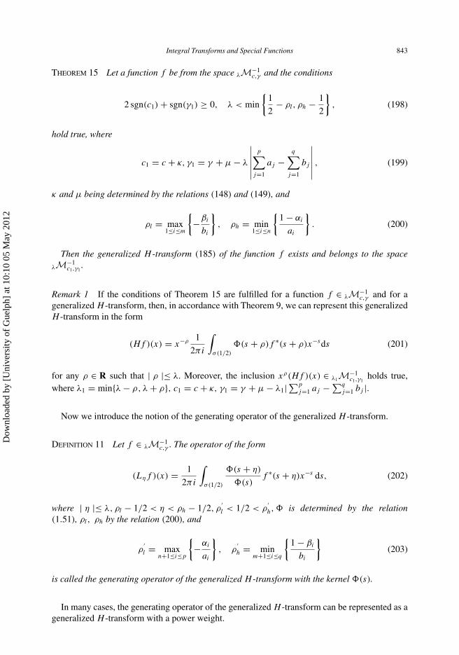
Integral Transforms and Special Functions 843
THEOREM 15 Let a function f be from the space λM−1c,γ and the conditions
2 sgn(c1) + sgn(γ1) ≥ 0, λ < min
{1
2− ρl, ρh − 1
2
}, (198)
hold true, where
c1 = c + κ, γ1 = γ + μ − λ
∣∣∣∣∣∣p∑
j=1
aj −q∑
j=1
bj
∣∣∣∣∣∣ , (199)
κ and μ being determined by the relations (148) and (149), and
ρl = max1≤i≤m
{−βi
bi
}, ρh = min
1≤i≤n
{1 − αi
ai
}. (200)
Then the generalized H -transform (185) of the function f exists and belongs to the spaceλM−1
c1,γ1.
Remark 1 If the conditions of Theorem 15 are fulfilled for a function f ∈ λM−1c,γ and for a
generalized H -transform, then, in accordance with Theorem 9, we can represent this generalizedH -transform in the form
(Hf )(x) = x−ρ 1
2πi
∫σ(1/2)
�(s + ρ)f ∗(s + ρ)x−sds (201)
for any ρ ∈ R such that | ρ |≤ λ. Moreover, the inclusion xρ(Hf )(x) ∈ λ1M−1c1,γ1
holds true,where λ1 = min{λ − ρ, λ + ρ}, c1 = c + κ, γ1 = γ + μ − λ1|∑p
j=1 aj −∑q
j=1 bj |.
Now we introduce the notion of the generating operator of the generalized H -transform.
DEFINITION 11 Let f ∈ λM−1c,γ . The operator of the form
(Lηf )(x) = 1
2πi
∫σ(1/2)
�(s + η)
�(s)f ∗(s + η)x−s ds, (202)
where | η |≤ λ, ρl − 1/2 < η < ρh − 1/2, ρ′l < 1/2 < ρ
′h, � is determined by the relation
(1.51), ρl, ρh by the relation (200), and
ρ′l = max
n+1≤i≤p
{−αi
ai
}, ρ
′h = min
m+1≤i≤q
{1 − βi
bi
}(203)
is called the generating operator of the generalized H -transform with the kernel �(s).
In many cases, the generating operator of the generalized H -transform can be represented as ageneralized H -transform with a power weight.
Dow
nloa
ded
by [
Uni
vers
ity o
f G
uelp
h] a
t 10:
10 0
5 M
ay 2
012
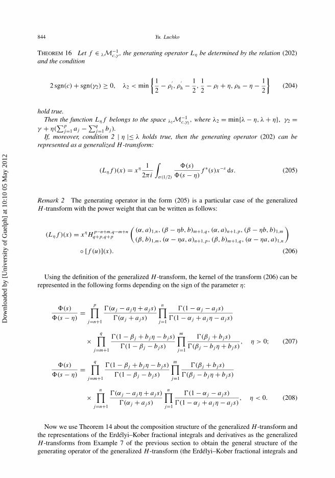
844 Yu. Luchko
THEOREM 16 Let f ∈ λM−1c,γ , the generating operator Lη be determined by the relation (202)
and the condition
2 sgn(c) + sgn(γ2) ≥ 0, λ2 < min
{1
2− ρ
′l , ρ
′h − 1
2,
1
2− ρl + η, ρh − η − 1
2
}(204)
hold true.Then the function Lηf belongs to the space λ2M−1
c,γ2, where λ2 = min{λ − η, λ + η}, γ2 =
γ + η(∑p
j=1 aj −∑q
j=1 bj ).If, moreover, condition 2 | η |≤ λ holds true, then the generating operator (202) can be
represented as a generalized H -transform:
(Lηf )(x) = xη 1
2πi
∫σ(1/2)
�(s)
�(s − η)f ∗(s)x−s ds. (205)
Remark 2 The generating operator in the form (205) is a particular case of the generalizedH -transform with the power weight that can be written as follows:
(Lηf )(x) = xηHp−n+m,q−m+nq+p,q+p
((α, a)1,n, (β − ηb, b)m+1,q , (α, a)n+1,p, (β − ηb, b)1,m
(β, b)1,m, (α − ηa, a)n+1,p, (β, b)m+1,q , (α − ηa, a)1,n
)◦ [f (u)](x). (206)
Using the definition of the generalized H -transform, the kernel of the transform (206) can berepresented in the following forms depending on the sign of the parameter η:
�(s)
�(s − η)=
p∏j=n+1
(αj − ajη + aj s)
(αj + aj s)
n∏j=1
(1 − αj − aj s)
(1 − αj + ajη − aj s)
×q∏
j=m+1
(1 − βj + bjη − bj s)
(1 − βj − bj s)
m∏j=1
(βj + bj s)
(βj − bjη + bj s), η > 0; (207)
�(s)
�(s − η)=
q∏j=m+1
(1 − βj + bjη − bj s)
(1 − βj − bj s)
m∏j=1
(βj + bj s)
(βj − bjη + bj s)
×n∏
j=n+1
(αj − ajη + aj s)
(αj + aj s)
n∏j=1
(1 − αj − aj s)
(1 − αj + ajη − aj s), η < 0. (208)
Now we use Theorem 14 about the composition structure of the generalized H -transform andthe representations of the Erdélyi–Kober fractional integrals and derivatives as the generalizedH -transforms from Example 7 of the previous section to obtain the general structure of thegenerating operator of the generalized H -transform (the Erdélyi–Kober fractional integrals and
Dow
nloa
ded
by [
Uni
vers
ity o
f G
uelp
h] a
t 10:
10 0
5 M
ay 2
012

Integral Transforms and Special Functions 845
derivatives Iγ,δ
β , Kτ,αβ , D
γ,δ
β , Pτ,αβ are defined by (154), (155), (166), (168), respectively):
(Lηf )(x) = xη
⎛⎝ m∏j=1
Pβj −bj η,bj η
1/bj
q∏j=m+1
D−βj ,bj η
1/bj
×n∏
j=1
I−αj ,aj η
1/aj
p∏j=n+1
Kαj −aj η,aj η
1/aj
⎞⎠ f (x), η > 0; (209)
(Lηf )(x) = xη
⎛⎝ n∏j=1
D−αj +aj η,−aj η
1/aj
p∏j=n+1
Pαj ,−aj η
1/aj
×m∏
j=1
Kβj ,−bj η
1/bj
q∏j=m+1
I−βj +bj η,−bj η
1/bj
⎞⎠ f (x), η < 0. (210)
Finally, we formulate the main theorem of this section that can serve as a tool for the solutionof some large classes of the differential, integral, and integro-differential equations involving thegenerating operators (for examples of these operators see the next section).
THEOREM 17 Let a function f belong to the space λM−1c,γ , a generalized H -transform possess
the kernel �, Lη be the generating operator of this generalized H - transform and the conditions
2 sgn(c) + sgn(γ2) ≥ 0, 2 sgn(c + κ) + sgn(μ + γ3) ≥ 0, 2 | η |≤ λ, (211)
λ2 < min
{1
2− ρ
′l , ρ
′h − 1
2,
1
2− ρl + η, ρh − η − 1
2,
1
2− ρl, ρh − 1
2
}, (212)
hold true, where
γ2 = γ + η
⎛⎝ p∑j=1
aj −q∑
j=1
bj
⎞⎠, γ3 = γ2 + μ − λ2
∣∣∣∣∣∣p∑
j=1
aj −q∑
j=1
bj
∣∣∣∣∣∣ ,λ2 = min{λ − η, λ + η},
κ, μ being determined by the relations (148) and (149), ρl, ρh by the relation (200) and ρ ′l , ρ
′h
by the relation (203).Then the following operational relation for the generalized H -transform holds true:
H(Lηf )(x) = xη(Hf )(x), (213)
that is, the generalized H -transform is a similarity, which translates the generating operator Lη
into the operation of multiplication by the power function xη.
Dow
nloa
ded
by [
Uni
vers
ity o
f G
uelp
h] a
t 10:
10 0
5 M
ay 2
012
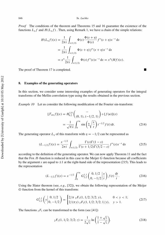
846 Yu. Luchko
Proof The conditions of the theorem and Theorems 15 and 16 guarantee the existence of thefunctions Lηf and H(Lηf ) . Then, using Remark 1, we have a chain of the simple relations:
H(Lηf )(x) = 1
2πi
∫σ(1/2)
�(s)�(s + η)
�(s)f ∗(s + η)x−s ds
= 1
2πi
∫σ(1/2)
�(s + η)f ∗(s + η)x−s ds
= xη 1
2πi
∫σ(1/2)
�(s)f ∗(s)x−s ds = xη(Hf )(x).
The proof of Theorem 17 is completed. �
8. Examples of the generating operators
In this section, we consider some interesting examples of generating operators for the integraltransforms of the Mellin convolution type using the results obtained in the previous section.
Example 10 Let us consider the following modification of the Fourier sin-transform:
[Fsmf ](x) = H1,00,2
( −(0, 1), (−1/2, 1)
)◦ [f (u)](x)
= 1√πx
∫ ∞
0sin
(2
√x
t
)t−1/2f (t) dt. (214)
The generating operator Lη of this transform with η = −1/2 can be represented as
(L−1/2f )(x) = x−1/2
2πi
∫σ(1/2)
(s)(1 − s)
(s + 1/2)(3/2 − s)f ∗(s)x−s ds (215)
according to the definition of the generating operator. We can now apply Theorem 11 and the factthat the Fox H -function is reduced in this case to the Meijer G-function because all coefficientsby the argument s are equal to ±1 at the right-hand side of the representation (215). This leads tothe representation
(L−1/2f )(x) = x−1/2∫ ∞
0G
1,12,2
(0, 1/2
0, −1/2
∣∣∣∣xt)
f (t)dt
t. (216)
Using the Slater theorem (see, e.g., [32]), we obtain the following representation of the MeijerG-function from the kernel of this transform:
G1,12,2
(y
∣∣∣∣ 0, 1/2
0, −1/2
)={
2/π 2F1(1, 1/2; 3/2; y), 0 < y < 1;2/(πy) 2F1(1, 1/2; 3/2; 1/y), y > 1.
(217)
The functions 2F1 can be transformed to the form (see [41])
2F1(1, 1/2; 3/2; z) = 1
2√
zln
(1 + √
z
1 − √z
). (218)
Dow
nloa
ded
by [
Uni
vers
ity o
f G
uelp
h] a
t 10:
10 0
5 M
ay 2
012

Integral Transforms and Special Functions 847
It follows from the relations (217) and (218) that
G1,12,2
(y
∣∣∣∣ 0, 1/2
0, −1/2
)= 1
π√
yln
(1 + √
y
| √y − 1 |
). (219)
The last relation, together with the representation (216) of the generating operator, leads to theformula:
(L−1/2f )(x) = 1
πx
∫ ∞
0ln
( √x + √
t
| √x − √
t |)
f (t)t−1/2 dt. (220)
Theorem 17 ensures that the modified Fourier sin-transform (214) and the integral operator withthe logarithmic kernel (220) are connected by means of the following operational relation:
[FsmL−1/2f ](x) = x−1/2[Fsmf ](x). (221)
Example 11 We define the modified Stieltjes transform as a particular case of the generalizedH -transform:
[Sαβ f ](x) = H
1,11,1
((α, β)
(α, β)
)◦ [f (u)] (x) =
∫ ∞
0
f (xtβ)t−α
1 + tdt. (222)
For α = 0, β = 1, the operator (222) coincides with the classical Stieltjes transform.The generating operator of the modified Stieltjes transform is given by
(Lηf )(x) = xη 1
2πi
∫σ(1/2)
(α + βs)(1 − α − βs)
(α + β(s − η))(1 − α − β(s − η))f ∗(s)x−s ds. (223)
The kernel of the operator (223) can be transformed with the help of the well-known supplementformula for the Euler -function:
(α + βs)(1 − α − βs)
(α + β(s − η))(1 − α − β(s − η))= sin(π(α − βη + βs))
sin(π(α + βs))
= cos(πβη) sin(π(α + βs)) − sin(πβη) cos(π(α + βs))
sin(π(α + βs))= cos(πβη) − sin(πβη)
× cos(π(α + βs))
sin(π(α + βs))= cos(πβη) − sin(πβη)
(α + βs)(1 − α − βs)
(1/2 + α + βs)(1/2 − α − βs). (224)
Substituting the representation (224) into formula (223), we arrive at the representation
(Lηf )(x) = xη(cos(πβη)f (x) − sin(πβη)[Hαβ f ](x)), (225)
where
[Hαβ f ](x) = H
1,12,2
((α, β),
(12 + α, β
)(α, β),
(12 + α, β
)) ◦ [f (u)] (x) = 1
π
∫ ∞
0
f (xtβ)t−α
t − 1dt (226)
is a generalized Hilbert transform (the integral in the right-hand side of the relation (226) isconsidered in the sense of the principal value). The generalized Hilbert transform coincides withthe classical Hilbert transform if α = 0 and β = 1.
Dow
nloa
ded
by [
Uni
vers
ity o
f G
uelp
h] a
t 10:
10 0
5 M
ay 2
012
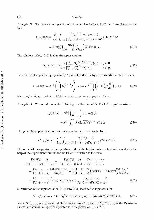
848 Yu. Luchko
Example 12 The generating operator of the generalized Obrechkoff transform (169) has theform
(Lηf )(x) = xη
2πi
∫σ( 1
2 )
∏nj=1 (1 − αj − aj s)∏n
j=1 (1 − αj − aj (s − η))f ∗(s)x−s ds
= xηH 0,nn,n
((α, a)1,n
(α − ηa, a)1,n
)◦ [f (u)] (x). (227)
The relations (209), (210) lead to the representation
(Lηf )(x) ={
xη(∏n
j=1 D−αj +aj η,−aj η
1/ajf)(x), η < 0;
xη(∏n
j=1 I−αj ,aj η
1/ajf)(x), η > 0.
(228)
In particular, the generating operator (228) is reduced to the hyper-Bessel differential operator
(Lηf )(x) = x−β
⎛⎝ n∏j=1
Dγj −1,1β f
⎞⎠ (x) = x−β
n∏j=1
(γj + 1
βx
d
dx
)f (x) (229)
if η = −β < 0, aj = −1/η = 1/β, 1 ≤ j ≤ n, and −αj = γj , 1 ≤ j ≤ n.
Example 13 We consider now the following modification of the Hankel integral transform:
[Jνf ](x) = G1,00,2
( −0, −ν
)◦ [f (u)] (x)
= xν/2∫ ∞
0Jν(2
√x/t)tν/2−1f (t) dt. (230)
The generating operator Lη of this transform with η = −ν has the form
(L−νf )(x) = x−ν
2πi
∫σ(1/2)
(s)(1 − s)
(1 + ν − s)(s + ν)f ∗(s)x−s ds. (231)
The kernel of the operator in the right-hand side of the last formula can be transformed with thehelp of the supplement formula for the Euler -function to the form:
(s)(1 − s)
(1 + ν − s)(s + ν)= (s)(1 − s)
(1 − ν − s)(s + ν)
(1 − s − ν)
(1 + ν − s)
= (1 − s − ν)
(1 + ν − s)
sin(π(s + ν))
sin(πs)= (1 − s − ν)
(1 + ν − s)
(cos(πν) + sin(πν)
cos(πs)
sin(πs)
)= (1 − s − ν)
(1 + ν − s)
(cos(πν) + sin(πν)
(s)(1 − s)
(1/2 − s)(1/2 + s)
). (232)
Substitution of the representation (232) into (231) leads to the representation
(L−νf )(x) = x−ν(x−νI 2ν
0+t−ν(cos(πν)f (t) + sin(πν)(H 01 f )(t))
)(x), (233)
where (H 01 f )(x) is a generalized Hilbert transform (226) and (xνI 2ν
0+t−νf )(x) is the Riemann–Liouville fractional integration operator with the power weights (156).
Dow
nloa
ded
by [
Uni
vers
ity o
f G
uelp
h] a
t 10:
10 0
5 M
ay 2
012
Integral Transforms and Special Functions 849
Example 14 The generating operator for the generalized Obrechkoff–Stieltjes transform (178)is called the mixed operator of the Erdélyi–Kober type (see [24]). This operator is a compositionof the Erdélyi–Kober fractional integrals and derivatives of the following form:
(Lηf )(x) ={
xη(∏m
i=1 Pβi−biη,biη
1/bi
∏ni=1 I
−αi ,aiη
1/aif )(x), η > 0,
xη(∏n
i=1 D−αi+aiη,−aiη
1/ai
∏mi=1 K
βi,−biη
1/bif )(x), η < 0,
(234)
where ai > 0, αi ∈ IR, i = 1, . . . , n; bi > 0, βi ∈ IR, i = 1, . . . , m. The mixed Erdélyi–Kobertype operator (234) is an ‘integral’ operator for η > 0 if
∑ni=1 ai >
∑mi=1 bi and for η < 0 if∑n
i=1 ai <∑m
i=1 bi . If∑n
i=1 ai <∑m
i=1 bi for η > 0 or∑n
i=1 ai >∑m
i=1 bi for η < 0 the operator(234) is a ‘differential’one. Finally, if
∑ni=1 ai =∑m
i=1 bi the mixed Erdélyi–Kober type operator(234) can be considered to be a generalization of the Hilbert integral transform.
Example 15 Finally, we consider the generalized Hankel transform (121). As it has been shownin [25,26], the generating operator for the generalized Hankel transform (121) can be representedas a particular case of the hyper-Bessel differential operators of even order 2m:
Bβ :=(
x
η
)−β 1
β2m
2m∏j=1
(x
d
dx+ βγj
). (235)
For a function f ∈ βM−1γ,0(L) the operational relation,
(HβBβf )(x) = (−1)mxβ(Hβf )(x) (236)
is fulfilled under the conditions
γ ≥ 2m; m
β≥ m +
2m∑j=1
γj ; γj >1
2β− 1, j = 1, . . . , m.
The operational relations for the generalized H -transforms and their generating operators, inparticular, those presented in Examples 10–15 can be used for solving linear equations containingthe generating operators by applying the corresponding integral transforms (see Section 2 fora general scheme how to do this). This method is often called an operational method. Anotherapproach to the solution of the same equations consists in the development of the operationalcalculus of the Mikusinski type and applying it for solving the corresponding equations. Wediscussed the idea of this method in Section 2. For the concrete realizations of this method forthe operators discussed in this paper (especially for those from the last section) the convolutionsof the corresponding integral transforms are required. The construction of the convolutions forthe generalized H -transform and for its different particular cases as well as different operationalcalculi of the Mikusinski type for various fractional calculus operators and their applications canbe found in [1,15–17,22,23,27–30,52].
References
[1] M.A. Al-Bassam andYu.F. Luchko, On generalized fractional calculus and its application to the solution of integro-differential equations, J. Fract. Calc. 7 (1995), pp. 69–88.
[2] L. Berg, Operational calculus in linear spaces, Studia Math. 20 (1961), pp. 1–18.[3] B.L.J. Braaksma andA. Schuitman, Some classes ofWatson transforms and related integral equations for generalized
functions, Siam. J. Math. Anal. 7 (1976), pp. 771–798.[4] R.V. Churchill, Operational Mathematics, McGraw-Hill, New York, 1958.
Dow
nloa
ded
by [
Uni
vers
ity o
f G
uelp
h] a
t 10:
10 0
5 M
ay 2
012

850 Yu. Luchko
[5] I.H. Dimovski, A transform approach to operational calculus for the general Bessel-type differential operator,C. R. Acad. Bulg. Sci. 27 (1974), pp. 155–158.
[6] ———, Convolutional Calculus, Publishing House of the Bulgarian Academy Sciences Sofia, 1982.[7] V.A. Ditkin and A.P. Prudnikov, Operational Calculus, Nauka, Moscow, 1975 (Russian).[8] G. Doetsch, Handbuch der Laplace-Transformation, Bd. I–IV, Birkhauser Verlag, Basel, 1950–1956.[9] A. Erdelyi, Operational Calculus and Generalized Functions, Holt, Rinehart and Winston, New York, 1962.
[10] A. Erdelyi, W. Magnus, F. Oberhettinger, and F.G. Tricomi, Higher Transcendental Functions, Vol. 1, McGraw-Hill,New York, 1953.
[11] ———, Tables of Integral Transforms, Vols. 1, 2, McGraw-Hill, 1953–1955.[12] M.A. Evgrafov, Series and integral representations, Itogi Nauki i Techniki, VINITI 13 (1986), pp. 5–92 (Russian).[13] M.V. Fedoryuk, Integral transforms, Itogi Nauki i Techniki, VINITI 13 (1986), pp. 211–253 (Russian).[14] C. Fox, The G- and H -functions as symmetrical Fourier kernels, Tran. Amer. Math. Soc. 98(3) (1961), pp. 395–429.[15] R. Gorenflo and Yu.F. Luchko, An operational method for solving fractional differential equations with the Caputo
derivatives. Acta Math. Vietnam. 24 (1999), pp. 207–233.[16] ———, Operational method for solving generalized Abel integral equations of second kind, Integral Transforms
Spec. Funct. 5 (1997), pp. 47–58.[17] R. Gorenflo, Yu.F. Luchko, and H.M. Srivastava, Operational method for solving integral equations with Gauss’s
hypergeometric function as a kernel, Inter. J. Math. Stati. Sci. 6 (1997), pp. 179–200.[18] I.H. Gradshteyn and I.M. Ryzhik, Tables of Integrals, Series, and Products, 6th edn, Academic Press, San Diego,
CA, 2000.[19] A.A. Kilbas and M. Saigo, H -transform. Theory and Applications, Chapman and Hall, Boca Raton, Florida,
2004.[20] A.A. Kilbas, H.M. Srivastava, and J.J. Trujillo, Theory and Applications of Fractional Differential Equations,
Elsevier, North-Holland, 2006.[21] H. Kober, On fractional integrals and derivatives, Q. J. Math. II Oxford, Ser. 11(1940), pp. 193–211.[22] Yu.F. Luchko, Operational method in fractional calculus, Fract. Calc. Appl. Anal. 2 (1999), pp. 463–489.[23] ———, Some operational relations for theH -transforms and their applications, Ph.D. thesis, Minsk, 1993 (Russian).[24] ———, Operational rules for a mixed operator of the Erdélyi-Kober type, Fract. Calc. Appl. Anal. 7 (2004),
pp. 339–364.[25] Yu.F. Luchko and V.S. Kiryakova, Hankel type transforms connected with the hyper-Bessel differential operators,
Proc. of Algebraic Analysis and Related Topics (Warsaw, 21–25 Sept.’99), Banach Center Publications (Inst. Math.PAN, Warsaw 2000) 53 (2000), pp. 155–165.
[26] ———, Generalized Hankel transforms for hyper-Bessel differential operators, C. R. Acad. Bulg. Sci. 53(8) (2000),pp. 17–20.
[27] Yu.F. Luchko and H.M.Srivastava, The exact solution of certain differential equations of fractional order by usingoperational calculus, Comput. Math. Appl. 29 (1995), pp. 73–85.
[28] Yu.F. Luchko and S.B. Yakubovich, Generating operators and convolutions for some integral transforms, Dokl.Akad. Nauk. BSSR. 35 (1991), pp. 773–776.
[29] ———, Convolutions for the generalized fractional integration operators, Proc. Intern. Conf. Complex Analysisand Appl. (Varna), Bulgarian Academy of Sciences (1993), pp. 199–211.
[30] ———, Operational method of solution of some classes of integro-differential equations, Differ. Uravn. 30 (1994),pp. 269–280.
[31] Y.L. Luke, The Special Functions and Their Approximations, Vols. 1, 2, Academic Press, NewYork, London, Tokyo,1969.
[32] O.I. Marichev, Handbook of Integral Transforms of Higher Transcendental Functions, Theory and AlgorithmicTables, Ellis Horwood, Chichester, 1983.
[33] A.M. Mathai, A Handbook of Generalized Special Functions for Statistical and Physical Sciences, Oxford UniversityPress, New York, 1993.
[34] A.M. Mathai and R.K. Saxena, Generalized hypergeometric functions with applications in statistics and otherdisciplines, Lecture Notes in Mathematics, 348, Springer-Verlag, Berlin, Heidelberg, New-York, 1973.
[35] ———, The H -Functions with Applications in Statistics and Other Disciplines, John Wiley, New York, London,Sydney, 1978.
[36] C.S. Meijer, Multiplikationstheoreme für die Funktion Gm,np,q (z), Proc. Nederl. Akad. Wet. 44 (1941), pp. 1062–1070.
[37] ———, On the G-function, I, II, III, IV, V, VI, VII, VIII, Proc. Nederl. Akad. Wet. 49 (1946), pp. 227–237, 344–356,457–469, 632–641, 765–772, 936–943, 1063–1072, 1165–1175.
[38] J. Mikusinski, Operational Calculus, Oxford University Press, Oxford, 1959.[39] F. Oberhettinger, Tables of Laplace Transforms, Springer-Verlag, New York, 1973.[40] ———, Tables of Mellin Transforms, Springer-Verlag, New-York, Heidelberg, Berlin, 1974.[41] A.P. Prudnikov,Yu.A. Brychkov, and O.I. Harichev, Integrals and Series, Volume 3: More special functions, Gordon
and Breach, New York, 1989.[42] ———, Evaluation of integrals and the mellin transform, Itogi Nauki Tekh. Ser. Mat. Analiz 27 (1989), pp. 3–146.[43] ———, Integrals and Series, Vol. 4 Direct Laplace Transforms, Gordon and Breach, New York, 1992.[44] ———, Integrals and Series, Vol. 5 Inverse Laplace Transforms, Gordon and Breach, New York, 1992.[45] S.G. Samko,A.A. Kilbas, and O.I. Marichev, Fractional Integrals and Derivatives: Theory and Applications, Gordon
and Breach, New York, 1993.[46] E.C. Titchmarsh, The zeros of certain integral functions, Proc. London Math. Soc. 25 (1926), pp. 283–302.
Dow
nloa
ded
by [
Uni
vers
ity o
f G
uelp
h] a
t 10:
10 0
5 M
ay 2
012

Integral Transforms and Special Functions 851
[47] ———, Introduction to theory of Fourier integrals, Oxford University Press, Oxford, 1937.[48] K.T. Vu, On the theory of generalized integral transforms in a certain function space, Dokl. AN SSSR 286 (19869),
pp. 521–524; J. Soviet Math 33 (1986), pp. 103–106 (English).[49] ———, Integral transforms and their composition structure, Dr.Sc. thesis, Minsk, 1987 (Russian).[50] K.T. Vu, O.I. Marichev, and S.B. Yakubovich, Composition structure of integral transformations, Dokl. AN SSSR
286 (1986), pp. 786–790; J. Soviet Math. 33 (1986), pp. 166–169 (English).[51] D.V. Widder, The Laplace Transform, Oxford University Press, Oxford, 1946.[52] S.B.Yakubovich andYu.F. Luchko, The Hypergeometric Approach to Integral Transforms and Convolutions, Kluwer,
Amsterdam, Netherlands, 1994.[53] K. Yosida, Operational Calculus: A Theory of Hyperfunctions, Springer-Verlag, Berlin, New York, 1984.
Dow
nloa
ded
by [
Uni
vers
ity o
f G
uelp
h] a
t 10:
10 0
5 M
ay 2
012