int. j. mathematics in operational research, vol. 10, no...
TRANSCRIPT

Int. J. Mathematics in Operational Research, Vol. 10, No. 2, 2017 229
Copyright © 2017 Inderscience Enterprises Ltd.
Multi-station manufacturing system analysis: theoretical and simulation study
Mohamed Boualem* Research Unit LaMOS (Modeling and Optimization of Systems), University of Bejaia, 06000 Bejaia, Algeria Fax: +213-34-21-51-88 Email: [email protected] *Corresponding author
Amina Angelika Bouchentouf Mathematics Laboratory, Department of Mathematics, Djillali Liabes University of Sidi Bel Abbes, 89, Sidi Bel Abbes 22000, Algeria Email: [email protected]
Mouloud Cherfaoui Department of Mathematics, University of Biskra, 07000, Algeria and Research Unit LaMOS (Modeling and Optimization of Systems), University of Bejaia, 06000 Bejaia, Algeria Email: [email protected]
Djamil Aïssani Research Unit LaMOS (Modeling and Optimization of Systems), University of Bejaia, 06000 Bejaia, Algeria Fax: +213-34-21-51-88 Email: [email protected]
Abstract: This paper deals with a flexible multi-station manufacturing system modelled by re-entrant queueing model. Our model incorporates classical queueing systems with exponential service times and controlled arrival process under a priority service discipline. The system is decomposed into N

230 M. Boualem et al.
fundamental multi-productive stations and 2N – 1 classes, a part follows the route fixed by the system, where each one is processed by N stations requiring 2N – 1 services. We assume that there is an infinite supply of work available, so that there are always parts ready for processing step 1. Our purpose in this paper is to present a detailed theoretical and simulation analysis of this priority multi-station manufacturing system.
Keywords: queues; manufacturing; priority scheduling policies; stability; modelling; virtual infinite buffers; simulation.
Reference to this paper should be made as follows: Boualem, M., Bouchentouf, A.A., Cherfaoui, M. and Aïssani, D. (2017) ‘Multi-station manufacturing system analysis: theoretical and simulation study’, Int. J. Mathematics in Operational Research, Vol. 10, No. 2, pp.229–260.
Biographical notes: Mohamed Boualem is a Lecturer at the Department of Technology, University of Bejaia, Algeria. He received his MS in Stochastic Methods of Operational Research from the USTHB, Algiers, Algeria, in 2003. He received his Doctorate degree in Applied Mathematics in 2009 and University Habilitation (HDR) in Mathematics in 2012 from University of Bejaia. He is a permanent researcher at the Research Unit LaMOS (Modeling and Optimization of Systems). His main current research interests include queueing theory, retrial queues, performance evaluation, stochastic orders, monotonicity, probability and statistics.
Amina Angelika Bouchentouf is a faculty member of Department of Mathematics, Djillali Liabes University of Sidi Bel Abbes, Algeria. She completed her PhD and University Habilitation (HDR) from the same university. Her research interests are in queueing theory, performance evaluation and stochastic orders.
Mouloud Cherfaoui is an Assistant Professor at the Department of Mathematics, Biskra University, Algeria. He received his MSc in Mathematics from Bejaia University, Algeria. He is a permanent researcher at the Research Unit LaMOS. His research interests include Markov chains and their stability, queuing theory, stochastic modelling and statistics.
Djamil Aïssani is a Full Professor of Mathematics at the Department of Operations Research at the University of Bejaia, Algeria. He started his career at the University of Constantine in 1978. He received his PhD in 1983 from Kiev State University (Soviet Union). He is at the University of Bejaia since its opening in 1983/1984. He is the Director of Research, Head of the Faculty of Science and Engineering (1999 to 2000), Director of the Research Unit LaMOS, and Scientific Head of the Computer Science Doctorate School ReSyD (2003 to 2011), and he has taught in many universities (USTHB Algiers, Annaba, Rouen, Dijon, ENITA, EHESS Paris, CNAM Paris, etc.). He has published many papers on Markov chains, queueing systems, reliability theory, performance evaluation and their applications in electrical, telecommunication networks and computer systems.
Multi-station manufacturing system analysis 231
1 Introduction
A manufacturing system can be defined as a combination of humans, machinery, and equipment that are bound by a common material and information flow. The materials input to a manufacturing system are raw materials and energy. Information is also input to a manufacturing system, in the form of customer demand for the system’s products. The outputs of a system can likewise be divided into materials, such as finished goods and scrap, and information, such as measures of system performance (Chryssolouris, 2006).
These sort of systems have been widely studied, Tiwari and Tiwari (2014) gave a novel methodology for sensor placement for the multi-station manufacturing processes so that the dimensional variation in the manufactured product will be reduced, Sangwan (2013) presented a criteria catalogue and a multi-criteria decision model for the evaluation of manufacturing systems based on environmental aspects of the manufacturing system, Fazlollahtabar and Saidi-Mehrabad (2013) developed a mathematical model to assess the reliability of machines and automated guided vehicles in flexible manufacturing systems, Polotski et al. (in press) analysed a failure prone manufacturing system producing two part types and requiring a setup for switching from one part type to another.
In recent years, queueing theory constitutes a powerful tool in modelling and performance analysis of many complex systems, such as production/flexible manufacturing systems, computer networks, telecommunication systems, call centres, and service systems. Many researchers focused on analysing these different machining systems, let us cite for instance, Jain (2013), Jain et al. (2013, 2014) and references therein.
Stability and performance analysis of multi-class queueing networks is by nowadays an agreeably-researched field. Some preeminent papers in this research field are Harrison (1988), Chen and Mandelbaum (1991), and Kumar (1993). Some notorious contributions with respect to the stability analysis can be summarised in Rybko and Stolyar (1992), Baccelli and Foss (1994), Dai (1995), Bramson (2008), Chen and Yao (2001), Meyn (2008) and Gurvich (2014).
Queueing networks with product form have been greatly studied, Visschers et al. (2011) considered a memoryless single station service system with many servers, authors showed that there exist assignment probabilities under which the system has a product form stationary distribution, and obtained explicit expressions for it, the waiting time distributions in steady state have been derived. Mather et al. (2011) showed for some multi-class queueing networks that time-dependent distributions for the multi-class queue lengths can have a factorised form which reduces the problem of computing such distributions to a similar problem for related single-class queueing networks. Jung and Morrison (2010) gave closed form solutions for the equilibrium probability distribution in the closed Lu-Kumar network under two buffer priority policies, Kim and Morrison (2010) presented an equilibrium probabilities in a class of two station closed queueing network.
Re-entrant lines [described in Harrison (1988)] are a special case of queueing models related with systems composed of some machines/stations, in which customers are processed several times by the same server. These schemes are used to model a variety of real life systems including service centres, production/manufacturing systems, computer
232 M. Boualem et al.
and communication networks…. Much attention has been devoted to obtain stability conditions for this kind of networks, Adan and Weiss (2005, 2006), Nazarathy and Weiss (2008), Weiss (2004, 2005) and Nazarathy (2008). A succinct study of these results is given in Guo et al. (2014), Kim and Morrison (2013), and Guo (2009).
Simulation technique is one of possible ways of modelling many complex systems. It can help to improve performance in terms of productivity, and most importantly it can help to identify and detect bottlenecks in production. Simulation has been used to study the behaviour of real systems in order to identify and understand problems associated with the systems. Therefore, in order to improve the performance in any manufacturing system, it is necessary to improve constraints also known as bottlenecks. Joseph and Sridharan (2014) focused on the evaluation of the routing flexibility of a flexible manufacturing system with the dynamic arrival of part types for processing in the system. A typical flexible manufacturing system configuration is chosen for detailed study and analysis. Ramaswami and Jeyakumar (2014) studied non-Markovian bulk queueing system with state dependent arrivals and multiple vacations using a simulation approach, Korytkowski and Wisniewski (2012) examined a multi-product production systems with in-line quality control, Rad et al. (2014) gave an analysis of a manufacturing system using simulation and multi-criteria decision-making tools were applied, Hasan et al. (2014) considered reconfigurable manufacturing systems to be one of the newer technologies which cannot only meet stochastic product demand but can also produce products having customised variety, Tajini et al. (2014) developed a flexible modelling environment for the simulation and analysis of different production systems, Boualem et al. (2015) focused on flexible production system modelled by re-entrant queueing network, where several performance measures have been investigated through expanded Monte Carlo simulations.
The main objective of this paper is to discuss the stability of a manufacturing system model under a specific service discipline, as an important source of the motivation of our research we mention Weiss (2004), where a stability analysis of a particular case ‘a re-entrant line with two stations and three processing steps’ of our general model is carried out. Thus, the main motivation of this research is to develop the stability study of general multi-station manufacturing system with an arbitrary N (N ≥ 2) number of stations by using two different techniques including fluid approach and Foster’s criterion. Note that it is not obvious how to extend the proofs beyond two machines queueing systems. In addition, in this paper the simulation is used to model our system. Using simulation technique as a means for improving existing manufacturing systems allows to evaluate the effect of local changes on the global system performance. The considered re-entrant model consists of N stations with infinite supply of work at the first one. In an infinite re-entrant line, we suppose that there are continually infinitely many class 1 customers available, which assures that the station serving class 1 will be always busy under non-idling service discipline.
Infinite supply of work expresses an ability to control the arrivals and is often a reasonable way to model a processing system. In some situations there may indeed be an infinite supply of work. In manufacturing systems, the supply of parts for processing at an expensive machine may be controlled and not allowed to exhaust. We refer to this as an infinite virtual queue: it acts like an infinite queue while in fact it only contains a few customers which are continually replenished. In standard queueing networks, one can regard the input stream as the output of a server which is fed by an infinite supply of work (Nazarathy and Weiss, 2010).

Multi-station manufacturing system analysis 233
Our system is a generalised infinite re-entrant line initialised by Weiss (2004). By using Foster criterion, the author gave a sufficient condition for the stability of the system. In the present work, we study stability condition for our system using Foster criterion and fluid approach, then the effects of various parameters on the performance of the system have been examined numerically.
This paper is organised as follows: Section 2 describes the manufacturing system modelled by a re-entrant queueing model. In Section 3, the theoretical analysis is given, the stability via fluid model approach and Foster criterion approach is established. In Section 4, a detailed simulation study is carried out considering two different specific policies, then the obtained results are compared.
2 The mathematical model
The multi-station manufacturing system considered in this paper consists of inputs, queues and servers as service centres (see Figure 1). Generally, it consists of N servers serving customers arriving in some manner and having some service requirements. The customers (the flow of entities) represent users, customers, transactions or programs. They arrive at the service facility for service, waiting for service, and leave the system after being served. The queueing system is described by distribution of inter-arrival times, distribution of service times, the number of servers, and the service discipline. More precisely we consider a multi-station manufacturing system model consisting of N stations, and a 2N – 1 steps. Customers arrive to the system at rate α, and follow the route fixed by the system, each one is processed first by station 1 for the first step with rate μ1, after that by station 2 for the second step with rate μ2, then aligns all the steps of the network, until the (2N – 1)th one at which it will be processed again by the first station with rate μ2N–1 then leaves definitively the system. The processing times for each of the 2N – 1 steps are independent sequences of independent identically distributed random variables, with means mi and rates 1 , 1,
ii mμ i N= = and without loss of generality we
scale time so that 1
1.N
iiμ
==∑ It is well-known that the customers arrive at this system in
a renewal stream, at rate α, and under the condition
( )2 1, 1, 1,1,
i i N i
N N
ρ m m i Nρ m
−⎧ = + < = −⎪⎨
= <⎪⎩
αα
(1)
the queues of customers waiting for each step are stable, and in fact the system is positive Harris recurrent, for any work conserving policy (see Dai and Weiss, 1996; Kumar and Kumar, 1994).
Assume that there is an infinite supply of work available, so that there are always customers ready for processing step 1. In this case, machine 1 will always be busy. In other words, the input and output rates at the first station are such that the offered load to all the resources is equal to ρ1 = 1. We call buffer 1 a virtual infinite queue. The queue is virtual because in practice buffer 1 need not contain many customers, but it needs to be monitored so it will never be empty. The concept of infinite supply of work is quite natural in many practical situations, and in particular it is very relevant to manufacturing systems. The fact that there are always infinitely many class 1 customers available

234 M. Boualem et al.
guarantees that the station serving class 1 will be always busy under non-idling service discipline.
Our purpose in this study is to discuss in details this system under last in first out policy (last buffer first server) (LIFO). In particular, we show that if m1 + m2N > mi + m2N–i, 2, 1i N= − and m1 + m2N > mN then under LIFO policy machine 1 will work all the time (that is we will have ρ1 = 1), but the queues for steps 2, 3, …, 2N – 1 will be stable. Suppose that in our system there are always customers available for processing of step 1. When these later finish processing step 1 by station 1, they queue in buffer 2 where they remain until they will be processed by machine 2 for step 2, then they move to machine 3 for step 3. The customers continue requiring services until they arrive to buffer N where they will be served by machine N for step N, after that they align the (N + 1)th queue requiring a service of mean mN+1 from the (N – 1)th station, and move to other stations for other services till the first one where they will be served with mean m2N–1, and finally they leave the system. Each buffer is processed in FIFO order. Processing is non-idling, that is a machine will always process a customer when there is work. We assume that machine i, 1, 1i N= − gives preemptive priority to buffer j, j = 2N – i. Whenever there are customers in buffer j, machine i will work on the first of them. When buffer j empties, machine i will immediately resume processing of a customer in step i. If during the processing of step i a customer arrives from buffer j – 1 into buffer j, machine i will preempt its work at buffer i, and immediately start processing buffer j. Since the processing times are exponential, this system can be described as a discrete state continuous time Markov jump process, with the state given by the number of customers in buffers 2, 2 1N − denoted n2, …, n2N–1.
Figure 1 Multi-station manufacturing model
Our result has an important practical applications in job-shop scheduling; the best realistic application of our model is job shop manufacturing system in which little batches of a variety of custom products are made. Job shops are usually businesses that perform custom parts manufacturing for other businesses. Examples of job shops include a large class of businesses a machine tool shop, a machining centre, a commercial printing shop, and many other manufacturers. Our model can be also found in many other realistic situations like communication network where each node transmits unlimited supply of materials and various classes of messages originating at this node, under some specific preemptive priority discipline. Metropolitan area networks is a particular computer communication case of our model, it is a network of ducting and fibre optic cable laid within a metropolitan area which can be used by a variety of businesses and organisations to provide services including telecom, internet access, television, etc.

Multi-station manufacturing system analysis 235
3 Theoretical study
The main objective of this paper is to discuss the stability conditions of our multi-station manufacturing system (see Figure 1). A sufficient condition for the stability of two machines and a three step production process, with an infinite supply of work was established in Weiss (2004) using the Foster criterion. In the current work, we give the condition stability of large class of general re-entrant line queueing networks initialised by Weiss (2004) using two different approaches, namely, the Foster criterion approach, and the fluid model approach. The main result is given in the following theorem.
Theorem 1: The multi-station manufacturing system with N stations and 2N – 1 processing step is stable if and only if
1 2 2
1 2
, 2, 1,.
N i N i
N N
m m m m i Nm m m
−⎧ + > + = −⎪⎨
+ >⎪⎩ (2)
Proof: The proof of this theorem will be given into two ways, the first one is based on Foster criterion approach, the second one on fluid model approach, but at first, let us give a succinctly explanation of the suggestion of equation (2). By hypothesis, the first queue is infinite virtual, this assumption assures that station 1 is working all the time, which means that the traffic intensity of the station is ρ1 = 1. So, every part which enter the system requires expected m1 + m2N time units from it. Station 1 is always busy, thus the number of parts which processes in the system per time unit is
1 21 .
Nm m+ Then for
2, ,j N= the number of parts that are processed when the station is fully utilised is mi +
mj, 2, 1,i N= − j = 2N – i and mN per time unit. To this end, it is reasonable to say that
the system will be stable if and only if m1 + m2N > mi + m2N–i, 2, 1,i N= − and m1 + m2N > mN.
The two following sub-sections establish the necessary and sufficient condition of our system, using two approaches.
3.1 First approach: the stability via foster criterion
In this part, we have to discuss the stability for Q(t) = (Qk), 2, 2 1k N= − by using the Foster criterion.
For our study, we need to employ the following result.
Lemma 2 (Meyn and Tweedie, 1993): Let h be a non-negative measurable function on state space of Markov chain Zn (the set of all non-negative integer numbers, it is written as S). S0 is a finite set of S.
The chain Zn is positive recurrent if there exist ε > 0 and B < ∞such that
( )( )1 0( ) for all .z h Z h z ε z S− < − ∉E (3)
( )( )1 0for all .z h Z B z S< ∈E (4)
Suppose that the non-negative function h satisfies

236 M. Boualem et al.
( )( )1 0( ) for all \ ,z h Z h z z S S≥ ∈E (5)
( )1 0 0sup ( ) if for any \ ,zz S
h Z h z z S S∈
− < ∞ ∈E (6)
( )0 0( ) for all ,h z h z z S> ∈ (7)
then we have 0( ) ,Sτ = ∞E where 0Sτ = inf{n ≥ Zn ∈ S0}. Now, we need to find a function h(∙) defined on S such that inequalities (3) to (4)
hold. Let h(n) = n, for all non-negative numbers. Let us prove that
1 2 1 2
1 2 1
, if 2, 1,,
N i N i
N N
m m m m i Nm m m
− −
−
⎧ + > + = −⎪⎨
+ >⎪⎩
is sufficient condition for the stability of process Q(t), in other words the Markov chain Zn is positive Harris recurrent.
We have, for z0 > L, with L the random number of customers processed in the each busy period of an M/M/1 queue with arrival rate μj and service rate μj+1, , 2 2;j N N= −
( )( ) ( ) ( )0
11 0 1
1 2 1.z i
N
mh Z h z μ μ Lm m −
′− ≤ −+
E E
:L′ number of customers served in a truncated busy period. Two cases are considered, either the busy period ends before all customers of class j are processed, and thus at that moment class j + 1 is empty, or class j empties the first.
We now choose ξ > 0 small enough, and define S0 = {0, 1, …, n2N–1}, so that for any z0 ∉ S0 we have:
( )( ) ( )01
1 0 11 2 1 2
0.iz i
N i N i
m mh Z h z μ μ ξm m m m− −
− ≤ − + <+ +
E
Thus, equation (3) holds and equation (4) follows directly from the definition of h(∙), this yields that Zs is positive recurrent.
Next, we need to find a function h(∙) defined on S such that inequalities (5) to (7) hold.
To prove the necessity of the stability conditions, we suppose that
1 2 1 2
1 2 1
, if 2, 1,,
N i N i
N N
m m m m i Nm m m
− −
−
⎧ + ≤ + = −⎪⎨
+ ≤⎪⎩
and we have to demonstrate that the Markov chain Zn is not positive Harris recurrent. So, for all z0 > n2N–1, and since m1 + m2N–1 ≤ mi + m2N–i, and m1 + m2N–1 ≤ mN we have
( )( ) ( )01
1 0 11 2 1 2
0.iz i
N i N i
m mh Z h z μ μm m m m− −
− ≥ − ≥+ +
E
Thus equation (5) holds. Now, for all z ∈ S

Multi-station manufacturing system analysis 237
( )( )2
11 1 1
1 2 1( ) .
N i
iz z i
N i m
m mh Z h z Z z μ μm m m −− +
− = − ≤ −+
E E
So, 1sup | ( ( )) ( ) | .z S z h Z h z∈ − < ∞E Then (6) holds. Equation (7) follows directly from the definition of h(∙), which completes the proof.
3.2 Second approach: the stability via fluid model
First, let us present some performance measures which are particularly interesting. Let 2N – 2 dimensional queue length process Q = (Qk) with Qk = {Qk(t): t ≥ 0}, where Qk(t) indicates the number of class k customers in the network at time t. The process S = {Sk(t), t ≥ 0}, where Sk(t) indicates the number of service completions for class k after station σ(k) serves k for a cumulative of t units of time. T = {Tk(t): t ≥ 0}, where Tk(t) indicates the cumulative amount of processing time that the station σ(k) has served class k customers during [0, t]. Thus, Sk(Tk(t)) is the total number of class k customer service completions by time t.
So, since there is a fixed route for all parts in the system, one can check that S(∙), T(∙), Y(∙) and Q(∙) satisfy the following queueing system:
( ) ( )1 1( ) (0) ( ) ( ) 0, 2, 2 1.k k k k k kQ t Q S T t S T t k N− −= + − ≥ = − (8)
[ ]( ) 00
( ) 1 , , 2 1.k
tk Q sT t ds k N N>= = −∫ (9)
[ ]22 2 ( ) 00
( ) ( ) ( ) 1 , 1, 1.N i
ti N i N i Q sT t t T t Y t ds i N−− − == − = = = −∫ (10)
[ ]( ) 00
( ) ( ) 1 .N
tN N Q sY t t T t ds== − = ∫ (11)
Then, referring to Chen (1995), and Dai and Weiss (1996), it is easy to verify that the fluid models corresponding to formulas (8)–(11) are given by:
( ) ( )1 1( ) (0) ( ) ( ) 0, 2, 2 1.k k k k k kQ t Q μ T t μ T t k N− −= + − ≥ = − (12)
[ ]( ) 00
( ) 1 , , 2 1.k
tk Q sT t ds k N N>= = −∫ (13)
[ ]22 2 ( ) 00
( ) ( ) ( ) 1 , 1, 1.N i
ti N i N i Q sT t t T t Y t ds i N
−− − == − = = = −∫ (14)
[ ]( ) 00
( ) ( ) 1 .N
tN N Q sY t t T t ds== − = ∫ (15)
Using formulas (13) to (15), Qk(∙) and Tk(∙), 1, 2 1,k N= − are Lipschitz continuous. Now, it is well-known that the fluid model given by expressions (12) to (15) is
strongly stable if there exists a time γ > 0 such that for any fluid solution Q(∙), T(∙) of the
fluid model with the initial condition 2 1
2(0) 1,
Nkk
Q−
==∑ we have
2 1
2( ) 0,
Nkk
Q t−
==∑ for
t ≥ γ.

238 M. Boualem et al.
To prove that our multi-station queueing model is stable, it suffices to prove that its corresponding fluid is stable, to this end, we have to demonstrate that the fluid model given by (12) to (15) is stable if and only if condition (2) is satisfied.
First, let us suppose that
1 2 2
1 2
, 2, 1,.
N i N i
N N
m m m m i Nm m m
−⎧ + ≤ + = −⎪⎨
+ ≤⎪⎩
By assumption, the first station is always busy, there is an infinitely customers waiting for service all the time, so 1 2 1( ) ( ) ,NT t T t t−+ = and 1 2 1( ) ( ) 1.NT t T t−+ =
Thus, for station 1 we have 1 2 11 1( ) 0.Nm m
m T t t−+ − ≥
The processing rate of class 1 is 1 1( ),μ T t such that
1 1 1 11 2 1 1 2 1
1 1( ) , and ( ) ,N N
μ T t t μ T tm m m m− −
≥ ≥+ +
Since for station 2, ,i N= we have 2( ) ( )i N iT t T t t−+ ≤ and ( ) ,NT t t≤ this yields
2
1 2 1 1 2 11 0, 0, and 1 0, 0.i N i N
N N
m m mt t t tm m m m
−
− −
+⎛ ⎞ ⎛ ⎞− ≥ ∀ > − ≥ ∀ >⎜ ⎟ ⎜ ⎟+ +⎝ ⎠ ⎝ ⎠
So, if mi + m2N–i ≥ m1 + m2N–1 and mN ≥ m1 + m2N–1, | ( ) |Q t → ∞ as t → ∞, with 2 1
1| ( ) | ( ).
Nkk
Q t Q t−
==∑ Thus, the necessity of the condition stability is proved.
Now, the necessary stability condition of the system turns out to be sufficient, it is simply to proceed by contra positive to get the sufficient result.
At first suppose that 2 1( ) 0,NQ t− ≠ this yield 1( ) 0,T t = and 2 1( ) 1.NT t− =
Thus, 2 1
2 11( ) .
Nk Nk
Q t μ−
−== −∑
If 2 1( ) 0, ( ) 0, 2, 2 1,N jQ t Q t j N− = ≠ = − and 2 1 2 1
1 2 1
( ) 0.i N i N
N
m m m mm m
− −
−
+ − ++ <
Since 2 1
2(0) 1
N
kQ
−
==∑ and Lipschitz continuity of
2 1
2( ),
N
kQ
−
=⋅∑ there exists a γ > 0
such that for t ≥ γ, 2 1
2( ) 0.
N
kQ t
−
==∑
Finally, we have proved that the fluid model given by formulas (12) to (15) associated with our network given by expressions (8) to (11) is stable, thus our manufacturing system is stable.
Next section is devoted to the simulation approach study, where a class of manufacturing system is modelled by a re-entrant queueing system to analyse its performance measures. In addition, we compare and verify the results obtained from the simulation techniques and the theoretical results given for this type of systems.

Multi-station manufacturing system analysis 239
4 Manufacturing system modelling and performance analysis
Consider a multi-station re-entrant manufacturing system composed of four stations and seven classes (see Figure 2), a prototype of a general model given in Section 2 (see Figure 1), customers arrive from outside requiring services, when these later finish processing step 1 by station 1, they align the second queue where they remain until they will be processed for step 2, after that they move to station 3 for the third service, and then to station 4 for the fourth one. Later, customers align the fifth queue requiring service of mean m5 from the third station, then continue requiring services from stations 2 and 1, afterwards they leave definitively the whole system. Stations 1, 2 and 3 give priority to buffer 7, 6 and 5 over buffer 1, 2, respectively.
Figure 2 Four station seven class manufacturing system
2
Station 2
1 4
Station 1
6 7
Station 4
3
Station 3
5
α
This system will be verified in order to ensure the theoretical result and finally analysis of the simulation model will be conducted. After the model is verified, there are different decisions that are made before the study proceeds any further. These include duration of the simulation, number of replication calculation, method of analysis used, etc. Finally, performance analysis and evaluation of the model and different operational procedures will be performed.
So, we analyse, evaluate and improve different performance measures of our system ‘The mean number of customers in the whole system and in each class, the mean number of customers waiting in the global system and in each station, and the load in the whole system and in each station’. Subsequently, we analyse the influence of parameters of the considered system for two specific policies:
• First policy: The arriving customers follow a Poisson process with rate α, service priority is given to class i, class 2N – i is not interrupted since it begins to be served.
• Second policy: This latter has been already defined in Section 2 (the mathematical model).
Throughout the analysis, several conclusions will be drawn by comparing the results obtained of the two policies. The primary objective of this part of paper is to model a class of multi-station manufacturing line, to analyse, to evaluate and improve its performance using computer simulation techniques. Finally, conclusions are drawn from the analysis made and then recommendations are given based on those

240 M. Boualem et al.
concluded points. Therefore, it is believed that the work will add some value to the existing knowledge. Analysis and evaluation of a multi-station manufacturing system usually uses performance indicators capable of assessing the adequacy of the model used with respect to the real system.
We first start by specifying performance measures which we consider interesting to study: In all what follows, we fixed Tmax = 20,000 time units (duration of the simulation) and MC = 100 (number of replication of Monte Carlo).
The following notations are used throughout this paper.
• Ni1, Ni2: The mean number of customers in the ith ( 1, 7)i = class in the case of the first and the second policy respectively.
• Qi1, Qi2: The mean number of customers in the queue of the ith ( 1, 7)i = class in the case of the first and the second policy respectively.
• Ci1, Ci2: The load (%) of the ith ( 1, 7)i = class in the case of the first and the second policy respectively.
• Ni1, Ni2 ( 8, 10) :i = The mean number of customers in the 1st, 2nd and 3d station in the case of the first and the second policy respectively.
• Qi1, Qi2 ( 8, 10) :i = The mean number of customers waiting in the first (resp. in the second) station in the case of the first and the second policy respectively.
• Ci1, Ci2 ( 8, 10) :i = The load (%) in the first (resp. in the second) station in the case of the first and the second policy respectively.
• N11,1, N11,2: The mean number of customers in the global system in the case of the first and the second policy respectively.
• Q11,1, Q11,2: The mean number of customers waiting in the global system in the case of the first and the second policy respectively.
• C11,1, C11,2: The load (%) of the global system in the case of the first and the second policy respectively.
First, let us fixed the service rates μi, ( 1, 7)i = and vary the arrival rates γ. Thereafter, we carry out inversely so as to obtain different states of the network.
4.1 First case: variation of the arrival rates α
For μi = 1/7, 1, 7,i = we vary α with a pitch equal to 0.01 starting with α = 0.05, for the two policies. The results are summarised in Tables 1 to 3.

Multi-station manufacturing system analysis 241
Table 1 Variation of the mean number of customers in the system in terms of α
α 0.0300 0.0500 0.0700 0.0900
αe 0.0738 0.0741 0.0739 0.0740 N11 0.4004 1.4426 15.3908 163.6631 N12 0.5180 0.5179 0.5176 0.5199 N21 0.3916 1.5115 16.0990 36.7867 N22 40.4849 35.9752 40.4291 37.5077 N31 0.3942 1.5689 13.3126 24.9258 N32 24.1205 27.5055 27.2439 26.9458 N41 0.2665 0.5773 1.0858 1.1549 N42 1.1492 1.1698 1.1564 1.1575 N51 0.3076 0.6742 1.1712 1.2338 N52 1.2411 1.2466 1.2465 1.2436 N61 0.3152 0.6894 1.2447 1.3158 N62 1.3300 1.3331 1.3326 1.3191 N71 0.3159 0.6969 1.2772 1.3819 N72 1.3881 1.3932 1.3913 1.3894 N81 0.7163 2.1395 16.6680 165.0450 N82 1.9062 1.9111 1.9089 1.9092 N91 0.7068 2.2008 17.3437 38.1024 N92 41.8150 37.3083 41.7617 38.8268 N10,1 0.7018 2.2431 14.4837 26.1597 N10,2 25.3616 28.7521 28.4904 28.1895 N11,1 2.3914 7.1607 49.5812 230.4620 N11,2 70.2319 69.1414 73.3173 70.0830
Table 2 Variation of the mean number of customers waiting in the system in terms of α
α 0.0300 0.0500 0.0700 0.0800
αe 0.0738 0.0741 0.0739 0.0738 Q11 0.1214 0.8799 14.4692 67.9457 Q12 0.0000 0.0000 0.0000 0.0000 Q21 0.1155 0.9466 15.1861 33.0355 Q22 39.5183 35.0080 39.4592 38.3486 Q31 0.1186 0.9998 12.4126 23.2096 Q32 23.1791 26.5561 26.2948 24.5111 Q41 0.0575 0.2298 0.6159 0.6535 Q42 0.6693 0.6877 0.6747 0.6681 Q51 0.0589 0.2199 0.5243 0.5575 Q52 0.5721 0.5744 0.5743 0.5740 Q61 0.0672 0.2487 0.6165 0.6607

242 M. Boualem et al.
Table 2 Variation of the mean number of customers waiting in the system in terms of α (continued)
Q62 0.6794 0.6822 0.6807 0.6856 Q71 0.0692 0.2620 0.6585 0.7229 Q72 0.7414 0.7472 0.7433 0.7398 Q81 0.2945 1.4425 15.7175 69.3034 Q82 0.9062 0.9111 0.9089 0.9072 Q91 0.2863 1.5038 16.3977 34.3246 Q92 40.8358 36.3287 40.7805 39.6738 Q10,1 0.2837 1.5457 13.5490 24.4103 Q10,2 24.3998 27.7854 27.5236 25.7364 Q11,1 1.5382 6.1744 48.5814 131.0905 Q11,2 69.2319 68.1414 72.3173 69.4109
Table 3 Variation of the load of the system in terms of α
α 0.0300 0.0500 0.0700 0.0800
αe 0.0738 0.0741 0.0739 0.0738 C11 27.9034 56.2669 92.1597 98.3781 C12 51.8036 51.7936 51.7620 51.8370 C21 27.6098 56.4846 91.2942 95.5056 C22 96.6659 96.7170 96.9885 96.8079 C31 27.5605 56.9101 90.0016 93.6947 C32 94.1472 94.9383 94.9073 94.5793 C41 20.8983 34.7421 46.9887 47.9379 C42 47.9867 48.2142 48.1625 48.0859 C51 24.8660 45.4305 64.6858 66.4758 C52 66.8971 67.2259 67.2148 66.9888 C61 24.8001 44.0694 62.8204 64.5011 C62 65.0587 65.0936 65.1888 65.1764 C71 24.6708 43.4941 61.8679 64.0160 C72 64.6784 64.5983 64.8022 64.8947 C81 42.1755 69.7075 95.0519 98.9062 C82 100.0000 100.0000 100.0000 100.0000 C91 42.0528 69.7033 94.5976 97.1743 C92 97.9106 97.9575 98.1130 98.0244 C10,1 41.8036 69.7345 93.4719 95.8436 C10,2 96.1802 96.6732 96.6763 96.4378 C11,1 85.3177 98.6319 99.9780 99.9940 C11,2 100.0000 100.0000 100.0000 100.0000

Multi-station manufacturing system analysis 243
According to Tables 1–3, we constant that:
• In the case of the first policy:
1 The mean number of customers (in the system and in the queues) is sensitive to the variation of α.
2 By varying α, the mean number of customers and the load in the classes 1 and 2 as in stations 1 and 2 increases considerably compared to other classes, so the first station will be congested which causes a congestion ‘bottleneck’ of the second station.
• In the case of the second policy:
1 There exists a considerable mean number of customers in the system and in the queue of each class.
2 For any α, compared to the first policy, the mean number of customers is more important in the second station. The load in the classes and in the stations 2 and 3 are equilibrated.
3 For α = 0.03, the load in the second station and in class 2 is very high compared to other classes, this latter will causes a saturation of station 3, this bottleneck is due to the fact that m1 + m7 = m2 + m6 = m3 + m5, [equation (2) is not verified].
Graphical representations (see Figure 3) illustrate the details of some results in the case of the first policy.
Figure 3 The state of the network when α = 0.08 and μ = [1/7, 1/7, 1/7, 1/7, 1/7, 1/7, 1/7] (see online version for colours)

244 M. Boualem et al.
Figure 3 The state of the network when α = 0.08 and μ = [1/7, 1/7, 1/7, 1/7, 1/7, 1/7, 1/7] (continued) (see online version for colours)
To conclude, we present a summary table on the results (see Table 4). This allows us to say that:
1 The network is unstable when one of the necessary conditions is not verified.
2 By varying α from 0.03 to 0.07, the system is stable in the case of the two policies (ρi < 1, 1, 4).i = On other hand, by varying α from 0.08 to 0.09, the system is
unstable (ρi > 1, 1, 3).i =

Multi-station manufacturing system analysis 245
Table 4 The state of the network in the case of the two policies
α ρ1 ρ2 ρ3 ρ4 Constatation
0.03 0.42 0.42 0.42 0.21 Stable 0.04 0.56 0.56 0.56 0.28 0.05 0.70 0.70 0.70 0.35 0.06 0.84 0.84 0.84 0.42 0.07 0.98 0.98 0.98 0.49 0.08 1.12 1.12 1.12 0.56 Unstable 0.09 1.26 1.26 1.26 0.63
4.2 Second case: variation of the service rates
4.2.1 Variation of the service rates of the first station
Let us vary the service rates μ1 and μ7, and fixed the rate α as the service rates of the second, the third and the fourth station. For α = 0.05, μ2 = 0.1, μ3 = 0.15, μ4 = 0.1, μ5 = 0.15 and μ6 = 0.2. The results of the simulation in the case of the two policies are summarised in Tables 5 to 7. Table 5 Variation of the mean number of customers in the system in terms of μ1 and μ7
μ1 0.2500 0.2000 0.1500 0.1000 μ7 0.0500 0.1000 0.1500 0.2000 αe 0.0426 0.0699 0.0845 0.0676 N11 83.1417 2.1207 1.2689 2.2128 N12 0.1699 0.3499 0.5611 0.6770 N21 5.6732 2.8849 2.2431 2.1444 N22 6.3445 60.0884 185.8040 30.6144 N31 1.5271 1.3659 1.2280 1.2364 N32 1.6018 5.0560 5.9585 4.8238 N41 1.0883 1.1272 1.0609 1.0667 N42 1.0861 2.3074 2.4475 2.2486 N51 0.5737 0.6414 0.6228 0.6297 N52 0.5886 1.0453 1.0846 1.0397 N61 0.5921 0.6708 0.6600 0.6498 N62 0.6087 1.1124 1.1585 1.0985 N71 4.4914 1.1130 0.6775 0.6825 N72 4.6337 2.1769 1.2861 1.1767 N81 87.6331 3.2337 1.9464 2.8953 N82 4.8036 2.5268 1.8472 1.8538

246 M. Boualem et al.
Table 5 Variation of the mean number of customers in the system in terms of μ1 and μ7 (continued)
N91 6.2654 3.5557 2.9031 2.7942
N92 6.9532 61.2008 186.9625 31.7129
N10,1 2.1008 2.0073 1.8508 1.8660
N10,2 2.1903 6.1014 7.0431 5.8636
N11,1 97.0875 9.9239 7.7613 8.6223
N11,2 15.0332 72.1364 198.3003 41.6789
Table 6 Variation of the mean number of customers waiting in the system in terms of μ1 and μ7
μ1 0.2500 0.2000 0.1500 0.1000
μ7 0.0500 0.1000 0.1500 0.2000
αe 0.0426 0.0699 0.0845 0.0676
Q11 82.1622 1.5175 0.7397 1.5407
Q12 0.0000 0.0000 0.0000 0.0000
Q21 5.1120 2.2175 1.5788 1.4795
Q22 5.7668 59.1165 184.8068 29.6484
Q31 1.0693 0.8333 0.7021 0.7067
Q32 1.1339 4.2576 5.1360 4.0287
Q41 0.6742 0.6270 0.5626 0.5652
Q42 0.6685 1.6571 1.7868 1.5972
Q51 0.2186 0.2194 0.2032 0.2056
Q52 0.2251 0.4676 0.4932 0.4635
Q61 0.2432 0.2521 0.2410 0.2303
Q62 0.2506 0.5274 0.5612 0.5176
Q71 3.6509 0.5764 0.2690 0.2735
Q72 3.7829 1.4479 0.6945 0.6115
Q81 86.6452 2.4889 1.2818 2.1414
Q82 3.8036 1.5268 0.8472 0.8538
Q91 5.6468 2.8097 2.1556 2.0453
Q92 6.3207 60.2214 185.9647 30.7368
Q10,1 1.5521 1.3458 1.1883 1.1983
Q10,2 1.6324 5.2340 6.1570 4.9968
Q11,1 96.0878 8.9296 6.7729 7.6326
Q11,2 14.0332 71.1364 197.3003 40.6789

Multi-station manufacturing system analysis 247
Table 7 Variation of the load of the system in terms of μ1 and μ7
μ1 0.2500 0.2000 0.1500 0.1000 μ7 0.0500 0.1000 0.1500 0.2000 αe 0.0426 0.0699 0.0845 0.0676 C11 97.9498 60.3274 52.9176 67.2133 C12 16.9894 34.9891 56.1078 67.7047 C21 56.1236 66.7418 66.4305 66.4924 C22 57.7720 97.1954 99.7163 96.6012 C31 45.7777 53.2558 52.5813 52.9699 C32 46.7848 79.8424 82.2512 79.5141 C41 41.4088 50.0126 49.8366 50.1474 C42 41.7577 65.0351 66.0729 65.1352 C51 35.5053 42.1999 41.9689 42.4062 C52 36.3444 57.7753 59.1420 57.6242 C61 34.8975 41.8650 41.9068 41.9525 C62 35.8115 58.5049 59.7296 58.0978 C71 84.0495 53.6568 40.8493 40.9059 C72 85.0794 72.9019 59.1633 56.5210 C81 98.7844 74.4812 66.4573 75.3980 C82 100.0000 100.0000 100.0000 100.0000 C91 61.8624 74.5914 74.7526 74.8883 C92 63.2502 97.9446 99.7810 97.6081 C10,1 54.8687 66.1481 66.2551 66.7718 C10,2 55.7938 86.7312 88.6102 86.6811 C11,1 99.9684 99.4264 98.8406 98.9624 C11,2 100.0000 100.0000 100.0000 100.0000
Following the numerical results given in Tables 5–7, we constat that:
• In the case of the first policy: 1 For μ = [0.25, 0.1, 0.15, 0.1, 0.15, 0.2, 0.05], the mean number of customers as
well as the load in the first class and in station 1, also in the overall system is very high compared to other classes, therefore the network is unstable. The instability is caused by the saturation of the first station (ρ1 > 1).
2 For (μ1, μ7) varying from (0.2, 0.1) to (0.15, 0.15), the mean number of customers decreases in the class i, 2, 7i = as in stations 1, 2, 3 and in the global system.
• In the case of the second policy: 1 For μ = [0.15, 0.1, 0.15, 0.1, 0.15, 0.2, 0.15], the mean number of customers and
the load in the second class and in the second station is very high, this later is due to the fact that equation (2) is not verified, m1 + m7 < m2 + m6.

248 M. Boualem et al.
2 For (μ1, μ7) varying from (0.25, 0.05) to (0.1, 0.2), the load of the first station and the global system is stable.
3 For (μ1, μ7) varying from (0.2, 0.1) to (0.15, 0.15), the mean number of customers increases.
For some results of Tables 5 to 7, graphical representations ‘in the case of the first policy’ are illustrated in Figures 4 and 5.
Figure 4 The state of the network when μ = [0.2, 0.1, 0.15, 0.1, 0.15, 0.2, 0.1] and α = 0.05 (see online version for colours)

Multi-station manufacturing system analysis 249
Figure 4 The state of the network when μ = [0.2, 0.1, 0.15, 0.1, 0.15, 0.2, 0.1] and α = 0.05 (continued) (see online version for colours)
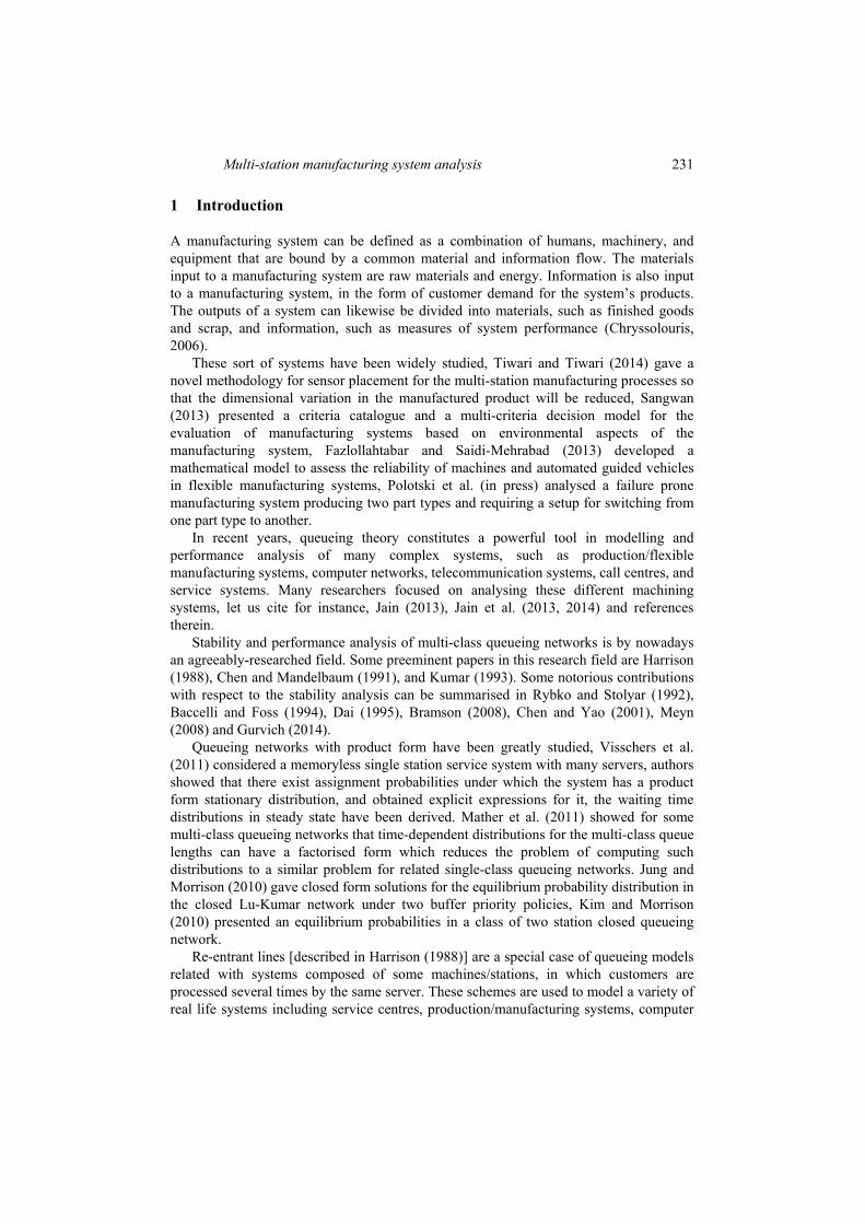
Figure 5 The state of the network when μ = [0.25, 0.1, 0.15, 0.1, 0.15, 0.2, 0.05] and α = 0.05 (see online version for colours)
250 M. Boualem et al.
Figure 5 The state of the network when μ = [0.25, 0.1, 0.15, 0.1, 0.15, 0.2, 0.05] and α = 0.05 (continued) (see online version for colours)
In conclusion, we present a summary table containing different situations of the network, based on its parameters. Table 8 permits us to constat that the state of the network is sensible to the variation of its parameters. Indeed, it moves from stability state (all conditions are fulfilled) to instability (if one of the conditions is not satisfied). For instance, when (μ2, μ6) = (0.25, 0.05), the network is unstable because (ρ1 = 1.2 > 1).

Multi-station manufacturing system analysis 251
Table 8 The state of the network by varying μ1 and μ7
μ1 μ7 ρ1 Constatation 0.25 0.05 1.2 Unstable 0.2 0.1 0.75 Stable 0.15 0.15 0.66 0.1 0.2 0.75
4.2.2 Variation of the service rates of the second station
Let us vary μ2 and μ6, fixed the arrival rate α, and the service rates of the first, the third and the fourth station. For α = 0.05, μ1 = 0.15, μ3 = 0.1, μ4 = 0.1, μ5 = 0.15 and μ7 = 0.15. In the case of the two policies, the simulation results are summarised in Tables 9 to 11. Table 9 Variation of the mean number of customers in the system in terms of μ2 and μ6
μ2 0.3000 0.2500 0.2000 0.1500 0.1000 μ6 0.0500 0.1000 0.1500 0.200 0.2500 αe 0.1074 0.0899 0.0902 0.0899 0.0905 N11 1.0587 1.2810 1.2275 1.2585 1.2831 N12 0.7152 0.6030 0.6006 0.6014 0.6020 N21 72.6008 1.6892 0.8582 0.9348 1.8614 N22 638.6951 22.7448 5.3407 8.3180 155.6400 N31 8.5491 4.5562 3.6572 3.4218 3.3426 N32 9.5928 283.3280 296.0426 291.3640 157.2491 N41 1.0470 1.1020 1.0601 1.0548 1.0312 N42 1.0871 1.7127 1.7155 1.7641 1.7052 N51 0.7706 0.8510 0.8231 0.8185 0.8140 N52 0.7986 0.8510 1.1866 1.1928 1.1827 N61 4.3566 1.0242 0.5903 0.4831 0.5680 N62 4.6594 1.5667 0.8934 0.7788 0.9188 N71 0.5167 0.6526 0.6472 0.6590 0.6838 N72 0.6843 1.0459 1.0637 1.0878 1.1197 N81 1.5754 1.9336 1.8747 1.9175 1.9670 N82 1.3995 1.6489 1.6644 1.6891 1.7217 N91 76.9573 2.7134 1.4485 1.4179 2.4294 N92 643.3545 24.3115 6.2341 9.0968 156.5587 N10,1 9.3197 5.4072 4.4803 4.2402 4.1566 N10,2 10.3914 284.5099 297.2292 292.5568 158.4318 N11,1 88.8994 11.1563 8.8637 8.6305 9.5841 N11,2 656.2326 312.1830 306.8431 305.1068 318.4175

252 M. Boualem et al.
Table 10 Variation of the mean number of customers in the queues in terms of μ2 and μ6
μ2 0.3000 0.2500 0.2000 0.1500 0.1000 μ6 0.0500 0.1000 0.1500 0.2000 0.2500 αe 0.1074 0.0899 0.0902 0.0899 0.0905 Q11 0.5670 0.7498 0.7021 0.7300 0.7525 Q12 0.0000 0.0000 0.0000 0.0000 0.0000 Q21 71.6255 1.1508 0.4358 0.4774 1.2416 Q22 637.6981 21.8258 4.5527 7.4597 154.6435 Q31 7.8819 3.7893 2.8961 2.6644 2.5850 Q32 8.9089 282.3325 295.0450 290.3666 156.2545 Q41 0.6264 0.6053 0.5629 0.5570 0.5346 Q42 0.6553 1.1167 1.1154 1.1616 1.1086 Q51 0.3185 0.3284 0.3042 0.3016 0.2967 Q52 0.3355 0.5323 0.5362 0.5417 0.5336 Q61 3.4967 0.4937 0.2090 0.1520 0.2042 Q62 3.7881 0.9075 0.3918 0.3159 0.4064 Q71 0.1635 0.2371 0.2359 0.2498 0.2791 Q72 0.2391 0.4778 0.4980 0.5275 0.5728 Q81 0.9588 1.2647 1.2111 1.2527 1.3029 Q82 0.3995 0.6489 0.6644 0.6891 0.7217 Q91 75.9715 2.0124 0.8648 0.8328 1.7306 Q92 642.3568 23.3649 5.3834 8.2021 155.5616 Q10,1 8.6145 4.5764 3.6480 3.4098 3.3252 Q10,2 9.6727 283.5134 296.2311 291.5587 157.4356 Q11,1 87.8995 10.1607 7.8726 7.6400 8.5913 Q11,2 655.2326 311.1830 305.8431 304.1068 317.4175
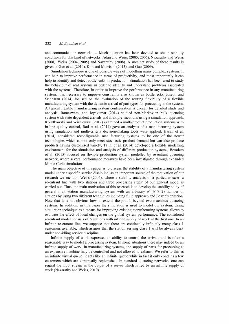
Table 11 Variation of the load of the system in terms of μ2 and μ6
μ2 0.3000 0.2500 0.2000 0.1500 0.1000 μ6 0.0500 0.1000 0.1500 0.2000 0.2500 αe 0.1074 0.0899 0.0902 0.0899 0.0905 C11 49.1684 53.1218 52.5445 52.8489 53.0629 C12 71.5172 60.2999 60.0637 60.1370 60.1982 C21 97.5310 53.8347 42.2434 45.7444 61.9838 C22 99.6968 91.8981 78.8088 85.8292 99.6431 C31 66.7137 76.6885 76.1054 75.7430 75.7628 C32 68.3900 99.5501 99.7589 99.7421 99.4593 C41 42.0638 49.6731 49.7235 49.7820 49.6546 C42 43.1798 59.5967 60.0038 60.2487 59.6664 C51 45.2146 52.2598 51.8902 51.6811 51.7297
Multi-station manufacturing system analysis 253
Table 11 Variation of the load of the system in terms of μ2 and μ6 (continued)
C52 46.3121 64.9582 65.0430 65.1050 64.9109 C61 85.9871 53.0533 38.1318 33.1047 36.3828 C62 87.1341 65.9186 50.1596 46.2909 51.2326 C71 35.3228 41.5530 41.1259 40.9190 40.4722 C72 44.5253 56.8093 56.5768 56.0267 54.6899 C81 61.6549 66.8929 66.3618 66.4738 66.4124 C82 100.0000 100.0000 100.0000 100.0000 100.0000 C91 98.5839 70.0996 58.3665 58.5150 69.8806 C92 99.7674 94.6594 85.0746 89.4648 99.7095 C10,1 70.5120 83.0829 83.2273 83.0392 83.1352 C10,2 71.8760 99.6542 99.8107 99.8047 99.6139 C11,1 99.9908 99.5598 99.1070 99.0451 99.2803 C11,2 100.0000 100.0000 100.0000 100.0000 100.0000
Following the numerical results given in Tables 9 to 11, we constat that:
• In the case of the second policy: 1 For (μ2, μ6) = (0.3, 0.05), the mean number of customers as well as the load in
the second class and in the second station in the case of the first policy is considerable and it is very high in the case of the second policy which causes a bottleneck in the overall system; equation (2) is not verified (m1 + m7 < m2 + m6).
2 For (μ2, μ6) varying from (0.25, 0.1) to (0.2, 0.15), the load is very high in the third class and the mean number of customers in the third station increases.
3 For (μ2, μ6) varying from (0.15, 0.2) to (0.1, 0.25), the mean number of customers deceases.
4 Whatever the variation of (μ2, μ6), the first station 1 and the global system are clogged which will also cause a congestion in the station 2.
• In the case of the first policy: For (μ2, μ4) varying from (0.25, 0.1) to (0.1, 0.25), the mean number of customers is almost equally distributed.
For some results of Tables 9 to 11, the graphs concerning the first policy are illustrated in Figures 6 and 7.

254 M. Boualem et al.
Figure 6 The state of the network when μ = [0.15, 0.25, 0.1, 0.1, 0.15, 0.1, 0.15] and α = 0.05 (see online version for colours)

Multi-station manufacturing system analysis 255
Figure 6 The state of the network when μ = [0.15, 0.25, 0.1, 0.1, 0.15, 0.1, 0.15] and α = 0.05 (continued) (see online version for colours)
Figure 7 The state of the network when μ = [0.15, 0.3, 0.1, 0.1, 0.15, 0.05, 0.15] and α = 0.05 (see online version for colours)
256 M. Boualem et al.
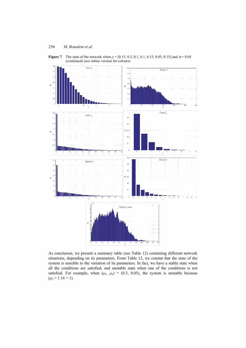
Figure 7 The state of the network when μ = [0.15, 0.3, 0.1, 0.1, 0.15, 0.05, 0.15] and α = 0.05 (continued) (see online version for colours)
As conclusion, we present a summary table (see Table 12) containing different network situations, depending on its parameters. From Table 12, we constat that the state of the system is sensible to the variation of its parameters. In fact, we have a stable state when all the conditions are satisfied, and unstable state when one of the conditions is not satisfied. For example, when (μ2, μ6) = (0.3, 0.05), the system is unstable because (ρ2 = 1.16 > 1).

Multi-station manufacturing system analysis 257
Table 12 The state of the system by varying μ2 and μ6 in the case of the two policies
μ2 μ6 ρ2 Constatation 0.30 0.05 1.60 Unstable 0.25 0.10 0.70 Stable 0.20 0.15 0.58 0.15 0.20 0.58 0.10 0.25 0.70
4.3 Concluding remarks for this section
• A detailed simulation of a type of multi-station manufacturing systems (four stations and seven classes) is presented, considering two disciplines.
• Using Monte Carlo techniques, the properties for system trajectories are well-established. The effectiveness of the proposed Monte Carlo algorithm is examined by a series of simulation experiments and is found to be gratifying.
• It is shown how perfect samples can be used to analyse and solve complex multi-server queue models, as well as to highlight selected properties and characteristics of them. The theoretical result given in Section 3 is illustrated and the effect of various parameters on the performance of the system have been examined.
• Simulation analysis from the stationary distributions should output information about the facial characteristics of any system, examples are information about bottlenecks.
5 Conclusions and final remarks
In the current paper, we present an analysis of a priority multi-station manufacturing system modelled by re-entrant controlled queueing system, these sort of systems are fundamental of study in operations research and applied probability as they provide sensible models for a variety of engineering, communications, telecommunication, and service situations. We establish the stability condition (condition 2) of Theorem 1 for our model by using Foster criterion and fluid approach. This is a generalisation of the result given by Weiss (2004).
In this present work, it is also demonstrated that a Monte Carlo simulation can be used to deal with this type of systems. From the preliminary analysis, it was shown that the simulation model is capable of analysing a complex multi-station manufacturing system. The model developed in this study was aimed to understand and improve the performances of the priority production system. From the results, it can be concluded that the performances obtained for a given system from our technique and theoretical results are very close to each other. Still the coherence in results obtained is very significant, hence it can be said that these techniques are applicable to any manufacturing system to evaluate and confirms its performances.
For further work, it is interesting to study our system with general processing times and investigate their potential in terms of performance. For a general re-entrant line with infinite supply of work, a general approach may be needed for hunting stable conditions.

258 M. Boualem et al.
Acknowledgements
The authors are grateful to the learned referees for their constructive comments and suggestions which helped a lot in the improvement of the quality and the clarity of the paper.
References Adan, I. and Weiss, G. (2005) ‘A two node Jackson network with infinite supply of work’,
Probability in the Engineering and Informational Sciences, Vol. 19, No. 2, pp.191–212. Adan, I. and Weiss, G. (2006) ‘Analysis of a simple Markovian re-entrant line with infinite supply
of work under the LBFS policy’, Queueing Systems, Vol. 54, No. 3, pp.169–183. Baccelli, F. and Foss, S. (1994) ‘Ergodicity of Jackson-type queueing networks’, Queueing
Systems, Vol. 17, No. 1, pp.5–72. Boualem, M., Cherfaoui, M., Bouchentouf, A.A. and Aïssani, D. (2015) ‘Modeling, simulation and
performance analysis of a flexible production system’, European Journal of Pure and Applied Mathematics, Vol. 8, No. 1, pp. 2–49.
Bramson, M. (2008) Stability of Queueing Networks, Springer, Berlin. Chen, H. (1995) ‘Fluid approximations and stability of multiclass queueing networks I:
work-conserving disciplines’, Annals of Applied Probability, Vol. 5, No. 3, pp.637–665. Chen, H. and Mandelbaum, A. (1991) ‘Discrete flow networks: bottleneck analysis and fluid
approximations’, Mathematics of Operations Research, Vol. 16, No. 2, pp.408–446. Chen, H. and Yao, D.D. (2001) Fundamentals of Queueing Networks: Performance, Asymptotics,
and Optimization, Springer, New York. Chryssolouris, G. (2006) Manufacturing Systems: Theory and Practice, Mechanical Engineering
Series, Springer New York. Dai, J.G. (1995) ‘On positive Harris recurrence of multiclass queueing networks: a unified
approach via fluid limit models’, Annals of Applied Probability, Vol. 5, No. 1, pp.49–77. Dai, J.G. and Weiss, G. (1996) ‘Stability and instability of fluid models for reentrant lines’,
Mathematics of Operations Research, Vol. 21, No. 1, pp.115–134. Fazlollahtabar, H. and Saidi-Mehrabad, M. (2013) ‘Optimising a multi-objective reliability
assessment in multiple AGV manufacturing system’, International Journal of Services and Operations Management, Vol. 16, No. 3, pp.352–372.
Guo, Y. (2009) ‘Fluid model criterion for instability of re-entrant line with infinite supply of work’, Top, Vol. 17, No. 2, pp.305–319.
Guo, Y., Lefeber, E., Nazarathy, Y., Weiss, G. and Zhang, H. (2014) ‘Stability of multi-class queueing networks with infinite virtual queues’, Queueing Systems, Vol. 76, No. 3, pp.309–342.
Gurvich, I. (2014) ‘Validity of heavy-traffic steady-state approximations in multiclass queueing networks: the case of queue-ratio disciplines’, Mathematics of Operations Research, Vol. 9, No. 1, pp.121–162.
Harrison, J.M. (1988) ‘Brownian models of queueing networks with heterogeneous customer populations’, in Fleming, W. and Lions, P.L. (Eds.): Stochastic Differential Systems, Stochastic Control Theory and Applications, pp.147–186, Springer, New York.
Hasan, F., Jain, P.K. and Kumar, D. (2014) ‘Performance modelling of dispatching strategies under resource failure scenario in reconfigurable manufacturing system’, International Journal of Industrial and Systems Engineering, Vol. 16, No. 3, pp.322–333.
Jain, M. (2013) ‘Transient analysis of machining systems with service interruption, mixed standbys and priority’, International Journal of Mathematics in Operational Research, Vol. 5, No. 5, pp.604–625.

Multi-station manufacturing system analysis 259
Jain, M., Sharma, G.C. and Mittal, R. (2014) ‘Queueing analysis and channel assignment scheme for cellular radio system with GPRS services’, International Journal of Mathematics in Operational Research, Vol. 6, No. 6, pp.704–731.
Jain, M., Shekhar, C. and Shukla, S. (2013) ‘Queueing analysis of two unreliable servers machining system with switching and common cause failure’, International Journal of Mathematics in Operational Research, Vol. 5, No. 4, pp.508–536.
Joseph, O.A. and Sridharan, R. (2014) ‘Simulation modelling and analysis of routing flexibility of a flexible manufacturing system’, International Journal of Industrial and Systems Engineering, Vol. 8, No. 1, pp.61–82.
Jung, S. and Morrison, J.R. (2010) ‘Closed form solutions for the equilibrium probability distribution in the closed Lu-Kumar network under two buffer priority policies’, in Proceeding of the 8th IEEE International Conference on Control and Automation, pp.1488–1495.
Kim, W-s. and Morrison, J.R. (2010) ‘On equilibrium probabilities in a class of two station closed queueing network’, in ICCAS2010: Proceeding of the International Conference on Control, Automation and System, pp.237–242.
Kim, W-s. and Morrison, J.R. (2013) ‘Non-product form equilibrium probabilities in a class of two-station closed reentrant queueing networks’, Queueing Systems, Vol. 73, No. 3, pp.317–339.
Korytkowski, P. and Wisniewski, T. (2012) ‘Simulation-based optimisation of inspection stations allocation in multi-product manufacturing systems’, International Journal of Advanced Operations Management, Vol. 4, Nos. 1–2, pp.105–123.
Kumar, P.R. (1993) ‘Re-entrant lines’, Queueing Systems, Vol. 13, No. 1, pp.87–110. Kumar, S. and Kumar, P.R. (1994) ‘Performance bounds for queueing networks and scheduling
policies’, IEEE Transactions on Automatic Control, Vol. 39, No. 8, pp.1600–1611. Mather, W.H., Hasty, J., Tsimring, L.S. and Williams, R.J. (2011) ‘Factorized time-dependent
distributions for certain multiclass queueing networks and an application to enzymatic processing networks’, Queueing Systems, Vol. 69, Nos. 3–4, pp.313–328.
Meyn, S.P. (2008) Control Techniques for Complex Networks, Cambridge University Press, Cambridge.
Meyn, S.P. and Tweedie, R.L. (1993) Markov Chains and Stochastic Stability, Springer-Verlag, London.
Nazarathy, Y. (2008) On Control of Queueing Networks and the Asymptotic Variance Rate of Outputs, PhD thesis, University of Haifa, Israïl.
Nazarathy, Y. and Weiss, G. (2008) ‘Near optimal control of queueing networks over a finite time horizon’, Annals of Operations Research, Vol. 170, No. 1, pp.233–249.
Nazarathy, Y. and Weiss, G. (2010) ‘Positive Harris recurrence and diffusion scale analysis of a push pull queueing network’, Performance Evaluation, Vol. 67, No. 4, pp.201–217.
Polotski, V., Kenné, J-P. and Gharbi, A. (in press) ‘Failure-prone manufacturing systems with setups: feasibility and optimality under various hypotheses about perturbations and setup interplay’, International Journal of Mathematics in Operational Research.
Rad, M.H., Sajadi, S.M. and Tavakoli, M.M. (2014) ‘The efficiency analysis of a manufacturing system by TOPSIS technique and simulation’, International Journal of Industrial and Systems Engineering, Vol. 18, No. 2, pp.222–236.
Ramaswami, K.S. and Jeyakumar, S. (2014) ‘Non-Markovian bulk queueing system with state dependent arrivals and multiple vacations-a simulation approach’, International Journal of Mathematics in Operational Research, Vol. 6, No. 3, pp.344–356.
Rybko, A.N. and Stolyar, A.L. (1992) ‘Ergodicity of stochastic processes describing the operation of open queueing networks’, Problems of Information Transmission, Vol. 28, No. 3, pp.199–220.
260 M. Boualem et al.
Sangwan, K.S. (2013) ‘Evaluation of manufacturing systems based on environmental aspects using a multi-criteria decision model’, International Journal of Industrial and Systems Engineering, Vol. 14, No. 1, pp.40–57.
Tajini, R., Elhaq, S.L. and Rachid, A. (2014) ‘Modelling methodology for the simulation of the manufacturing systems’, International Journal of Simulation and Process Modelling, Vol. 9, No. 4, pp.285–305.
Tiwari, P. and Tiwari, M.K. (2014) ‘Knowledge driven sensor placement in multi-station manufacturing processes’, International Journal of Intelligent Engineering Informatics, Vol. 2, Nos. 2–3, pp.118–138.
Visschers, J., Adan, I. and Weiss, G. (2011) A Product Form Solution to a System with Multi-type Jobs and Multitype Servers, Eurandom report, 2011–002.
Weiss, G. (2004) ‘Stability of a simple re-entrant line with infinite supply of work-the case of exponential processing times’, Journal Operations Research Society of Japan, Vol. 47, No. 4, pp.304–313.
Weiss, G. (2005) ‘Jackson networks with unlimited supply of work’, Journal of Applied Probability, Vol. 42, No. 3, pp.879–882.