instrumentation platform and maximum power point...
TRANSCRIPT

Ramsay Rafaël Mac Donald
Instrumentation platform and Maximum Power
Point Tracking control for a Hydrokinetic turbine
Brasilia-DF
2017

Ramsay Rafaël Mac Donald
Instrumentation platform and Maximum Power Point
Tracking control for a Hydrokinetic turbine
Universidade de Brasília – UnB
Faculdade de Tecnologia
Programa de Pós-Graduação
Supervisor: Dr. Rudi Henri van Els
Brasilia-DF
2017

Ramsay Rafaël Mac DonaldInstrumentation platform and Maximum Power Point Tracking control for a Hydrokinetic
turbine/ Ramsay Rafaël Mac Donald. – Brasilia-DF, 2017-134 p. : il. (algumas color.) ; 30 cm.
Supervisor: Dr. Rudi Henri van Els
Dissertation (Masters) – Universidade de Brasília – UnBFaculdade de TecnologiaPrograma de Pós-Graduação, 2017.
1. Hydrokinetic turbine. 2. Instrumentation. 2. Maximum Power Point Tracking. I. R. Els.II. Universidade de Brasília. III. Faculdade de Tecnologia. IV. Instrumentation platform andMaximum Power Point Tracking control for Hydrokinetic turbine.

Ramsay Rafaël Mac Donald
Instrumentation platform and Maximum Power PointTracking control for a Hydrokinetic turbine
Trabalho aprovado. Brasilia-DF, 4 de Abril, 2017:
Dr. Rudi Henri van ElsOrientador
Dr. Daniel Mauricio Muñoz ArboledaConvidado 1
Dr. Antônio Cesár Pinho Brasil JuniorConvidado 2
Brasilia-DF2017

Acknowledgements
To my parents, my brother, and my family for their love and support.
To my colleagues and friends at the laboratory: Aramis, Eugenia, Francis, Francisco, Giselle,Miguel, Nela, Paulo, Rafael, and Vinicius for their moral and academic support, and for thepleasant working environment they have created.
To my friends in Brazil, for sharing their families and culture with me, be it Brazilian, Colom-bian, or Cuban.
To my supervisor Dr. Rudi van Els, who took the initiative to create cooperation betweenthe Surinamese University and the University of Brasilia, and dragged me to Brazil duringmy undergrad and has kept guiding me through my master’s. May you keep guiding moreSurinamese students into higher education.
To Dr. Antônio Brasil Junior for the guidance, patience, and the opportunity to participate inthe hydrokinetic turbine development project Hydro-K.
To the SuriBraz Academic Network, for the guidance and support.
To AES who has supported this work.

Abstract
A project named Hydro-K is aimed at developing a hydrokinetic turbine. The prototype orpreliminary model of this turbine will inherently present uncertainties. Eliminating themrequires testing and data gathering. The data is acquired using an instrumentation platformdesigned in this dissertation. Another challenge will be controlling the turbine. Controllingtraditional horizontal-axis-variable-speed-fixed-pitch hydrokinetic turbines requires mappingits efficiency at various water and rotor speeds, i.e., the CP curve of the turbine, in advance.Whereafter, its rotational velocity is measured and manipulated in order to maintain maximumefficiency of the rotor. Recently, Maximum Power Point Tracking (MPPT) control has beenapplied to wind turbines. This control method eliminates the necessity of CP curve mapping bymeasuring the generator’s voltage and current output, and periodically adjusting the electricalload on the generator to maintain the maximum electrical power output. Considering thesimilarities between hydrokinetic and wind turbines, it is likely that MPPT can be effectivelyapplied for the hydrokinetic variant. Therefore, a second objective is assessing the effectivenessof MPPT for hydrokinetic turbines by comparing a conventional control strategy with MPPTusing simulations in "SIMULINK". The electrical load on the generator is varied by usingPulse Width Modulation (PWM). The Hydro-K turbine developed at the University of Brasilia(UnB) is equipped with a three-phase-permanent-magnet-synchronous- generator (PMSG). Theresults of the simulations are presented by comparing the two aforementioned control methodsunder different water velocity conditions, and show that MPPT control delivers a superiorelectrical output.
Keywords: hydrokinetic turbine. instrumentation. maximum power point tracking.

Resumo
O projeto Hydro-K tem como objetivo o desenvolvimento de uma turbina hidrocinética. Oprotótipo ou o modelo preliminar desta certamente apresenta incertezas e para eliminá-las sãonecessários testes e coleta de dados. Essa coleta foi feita através de uma plataforma instrumentaldesenvolvida neste trabalho. Um outro desafio foi o controle da turbina. O controle tradicionaldas turbinas hidrocinéticas com um eixo horizontal, velocidade variável e um angulo da páfixo, requer o mapeamento da curva CP da turbina com antecedência. Em seguida, a suavelocidade de rotação é medida e manipulada de modo a manter a máxima eficiência dorotor. Recentemente, o controle do Maximum Power Point Tracking (MPPT) foi aplicado àsturbinas eólicas. Esse método de controle elimina a necessidade de mapeamento de curva CP
medindo a tensão e a saída de corrente do gerador e ajustando periodicamente a carga elétricano gerador para manter a potência máxima de saída elétrica. Considerando as semelhançasentre as turbinas hidrocinéticas e as eólicas, é provável que o MPPT possa ser aplicado paraos hidrogeradores. Um segundo objetivo desta dissertação é avaliar a eficácia do MPPT paraturbinas hidrocinéticas comparando uma estratégia de controle convencional com o MPPTusando simulações no "SIMULINK". A carga elétrica no gerador é variada usando o Pulse
Width Modulation (PWM). A turbina hidrocinética do Hydro-K desenvolvida na Universidadede Brasília (UnB) é equipada com um gerador síncrono-trifásico com ímã permanente. Osresultados das simulações e experiências são apresentados comparando os dois métodos decontrole acima mencionados sob diferentes condições de velocidade da água, e mostram que ocontrole MPPT fornece uma saída elétrica superior.
Palavras-chave: turbina hidrocinética. instrumentação. maximum power point tracking.

List of Figures
Figure 1 – Comparative primary energy consumption with renewables accounting for7.83% in 2010, and 9.57% of the total energy consumption in 2015. . . . . 16
Figure 2 – Various wave energy conversion systems. . . . . . . . . . . . . . . . . . . 21Figure 3 – Classification of hydrokinetic energy converters . . . . . . . . . . . . . . 22Figure 4 – Example of a CP-λ curve. . . . . . . . . . . . . . . . . . . . . . . . . . . 23Figure 5 – Main control systems of a hydrokinetic energy converter. . . . . . . . . . 25Figure 6 – Generation 1 turbine source: Els et al. (2003). . . . . . . . . . . . . . . . 27Figure 7 – Control schematic for the Generation 1 HKT. . . . . . . . . . . . . . . . . 28Figure 8 – Control schematic for the Generation 1 HKT. With an automatically con-
trolled stator excitation. . . . . . . . . . . . . . . . . . . . . . . . . . . . 28Figure 9 – Generation 2 turbine source: Brasil Jr. et al. (2007). . . . . . . . . . . . . 29Figure 10 – Control schematic for the Generation 2 HKT. . . . . . . . . . . . . . . . . 30Figure 11 – Generation 3 turbine source: Brasil Jr. et al. (2007). . . . . . . . . . . . . 30Figure 12 – Control schematic for the Generation 3 HKT. . . . . . . . . . . . . . . . . 31Figure 13 – Tucunaré turbine concept. . . . . . . . . . . . . . . . . . . . . . . . . . . 31Figure 14 – Different arrangements of HK-10 turbines. . . . . . . . . . . . . . . . . . 32Figure 15 – General overview of the instrumentation and control schematic for the
HK-10 turbine. . . . . . . . . . . . . . . . . . . . . . . . . . . . . . . . . 33Figure 16 – Conceptual instrumentation and control schematic for the HK-10 turbine. . 34Figure 17 – Product life cycle. . . . . . . . . . . . . . . . . . . . . . . . . . . . . . . 37Figure 18 – Kano diagram of client satisfaction with requirements. . . . . . . . . . . . 41Figure 19 – Global function of the product. . . . . . . . . . . . . . . . . . . . . . . . 45Figure 20 – Partial functions of the product. . . . . . . . . . . . . . . . . . . . . . . . 46Figure 21 – Elementary functions of the 1st alternative functional model. . . . . . . . 47Figure 22 – Elementary functions of the 2nd alternative functional model. . . . . . . . 48Figure 23 – Elementary functions of the 3rd alternative functional model. . . . . . . . 49Figure 24 – Dominant flow heuristic applied to a functional structure. . . . . . . . . . 54Figure 25 – Branching flow heuristic applied to a functional structure. . . . . . . . . . 55Figure 26 – Conversion—transmission heuristic applied to a functional structure. . . . 55Figure 27 – Concept 1. PLC for data processing . . . . . . . . . . . . . . . . . . . . . 56Figure 28 – Concept 2. Microprocessor as data processor . . . . . . . . . . . . . . . . 57Figure 29 – Concept 3. Microcontroller as data processor . . . . . . . . . . . . . . . . 57
Figure 30 – Instrumentation requirements for the Hydro-K project . . . . . . . . . . . 59Figure 31 – Signal conditioning for current transformer . . . . . . . . . . . . . . . . . 61Figure 32 – Schematic of the designed voltage divider . . . . . . . . . . . . . . . . . 62Figure 33 – Schematic for designed water flow sensor . . . . . . . . . . . . . . . . . 64Figure 34 – Finite State Machine diagram for program . . . . . . . . . . . . . . . . . 66Figure 35 – Instrumentation platform testing on lathe . . . . . . . . . . . . . . . . . . 68Figure 36 – Results of tests on the lathe . . . . . . . . . . . . . . . . . . . . . . . . . 69Figure 37 – Instrumentation testing on water . . . . . . . . . . . . . . . . . . . . . . 70Figure 38 – I-V and P-V curves for PV systems. . . . . . . . . . . . . . . . . . . . . 72Figure 39 – Flowchart of MPPT algorithm by Zhou (2012). . . . . . . . . . . . . . . 75Figure 40 – Flowchart of MPPT algorithm by Mofei (2014). . . . . . . . . . . . . . . 76Figure 41 – Slope on the P-V curve . . . . . . . . . . . . . . . . . . . . . . . . . . . 77Figure 42 – Flowchart of MPPT algorithm by the author . . . . . . . . . . . . . . . . 78Figure 43 – Simplified block diagram of simulation model . . . . . . . . . . . . . . . 79Figure 44 – Simulink model of the CP curve and mechanical torque output. . . . . . . 80Figure 45 – Simulink physical signal gear box model. . . . . . . . . . . . . . . . . . . 81Figure 46 – Simulink PMSG subsystem. . . . . . . . . . . . . . . . . . . . . . . . . . 82Figure 47 – Simulink filtering and processing power data subsystem. . . . . . . . . . . 83Figure 48 – Simulink fixed average filter subsystem. . . . . . . . . . . . . . . . . . . 83Figure 49 – Linearization of the resistance determined by the algorithm, and the neces-
sary duty cycle . . . . . . . . . . . . . . . . . . . . . . . . . . . . . . . . 83Figure 50 – Block diagram of the MPPT control model . . . . . . . . . . . . . . . . . 84Figure 51 – Model of MPPT control algorithm by Zhou (2012) . . . . . . . . . . . . . 84Figure 52 – Model of MPPT control algorithm by Mofei (2014) . . . . . . . . . . . . 84Figure 53 – Block diagram of the optimalω control model . . . . . . . . . . . . . . . 85Figure 54 – Model of MPPT control algorithm by Mac Donald (2017) . . . . . . . . . 86Figure 55 – Calculation of the referenceω . . . . . . . . . . . . . . . . . . . . . . . 86Figure 56 – Complete model of the hydrokinetic turbine with MPPT control . . . . . . 87Figure 57 – Complete model of the hydrokinetic turbine optimal usingω control with PID 88Figure 58 – Temperature data . . . . . . . . . . . . . . . . . . . . . . . . . . . . . . 90Figure 59 – Vibration data . . . . . . . . . . . . . . . . . . . . . . . . . . . . . . . . 91Figure 60 – Battery voltage . . . . . . . . . . . . . . . . . . . . . . . . . . . . . . . . 91Figure 61 – Rotor rotational velocity data . . . . . . . . . . . . . . . . . . . . . . . . 92Figure 62 – Power data . . . . . . . . . . . . . . . . . . . . . . . . . . . . . . . . . . 93Figure 63 – River velocity input . . . . . . . . . . . . . . . . . . . . . . . . . . . . . 94Figure 64 – Comparison of resulting CP at various river velocities . . . . . . . . . . . 95

Figure 65 – Comparison of resulting generator power output at various river velocities 95Figure 66 – Comparison of resulting electrical resistance change at various river velocity
conditions . . . . . . . . . . . . . . . . . . . . . . . . . . . . . . . . . . 96Figure 67 – Schematic for the instrumentation platform . . . . . . . . . . . . . . . . . 111Figure 68 – ESP8266 WiFi shield complete with RTC and SD-Card as replacement for
CC3000 WiFi shield . . . . . . . . . . . . . . . . . . . . . . . . . . . . . 112Figure 69 – The first instrumentation prototype for a single Hydro-K turbine . . . . . 113Figure 70 – The second instrumentation prototype for a single Hydro-K turbine . . . . 114Figure 71 – The first instrumentation prototype for all three Hydro-K turbines . . . . . 115Figure 72 – Current transformer’s signal conditioning PCB . . . . . . . . . . . . . . . 116Figure 73 – Voltage sensor with selectable resolution . . . . . . . . . . . . . . . . . . 117Figure 74 – PCB of designed water flow sensor . . . . . . . . . . . . . . . . . . . . . 118Figure 75 – Calibration curve of the river velocity sensor (impeller) . . . . . . . . . . 133Figure 76 – Calibration curve of the digital temperature sensors . . . . . . . . . . . . 133Figure 77 – Calibration curve of current transformers . . . . . . . . . . . . . . . . . . 134Figure 78 – Calibration curve of the voltage dividers . . . . . . . . . . . . . . . . . . 134

List of Tables
Table 1 – List of Stakeholders with their classification. . . . . . . . . . . . . . . . . 36Table 2 – Full list of client sub requirements, grouped into main client requirements. . 38Table 3 – Mudge diagram of the platform’s functions. . . . . . . . . . . . . . . . . . 39Table 4 – Results mudge diagram of customer function requirements. . . . . . . . . . 40Table 5 – Product requirements in accordance with the client requirements . . . . . . 42Table 6 – Quality Function Deployment for product features. . . . . . . . . . . . . . 43Table 7 – Product requirements. . . . . . . . . . . . . . . . . . . . . . . . . . . . . 44Table 8 – Selection matrix for the functional structure . . . . . . . . . . . . . . . . . 50Table 9 – Selection matrix for the functional structure . . . . . . . . . . . . . . . . . 53Table 10 – Product concept selection matrix . . . . . . . . . . . . . . . . . . . . . . . 58Table 11 – Selected components of the product concept . . . . . . . . . . . . . . . . . 58Table 12 – Legend for Finite State Machine diagram displayed above . . . . . . . . . 66Table 13 – Selection matrix for sensors . . . . . . . . . . . . . . . . . . . . . . . . . 107Table 14 – Pin reference . . . . . . . . . . . . . . . . . . . . . . . . . . . . . . . . . 110
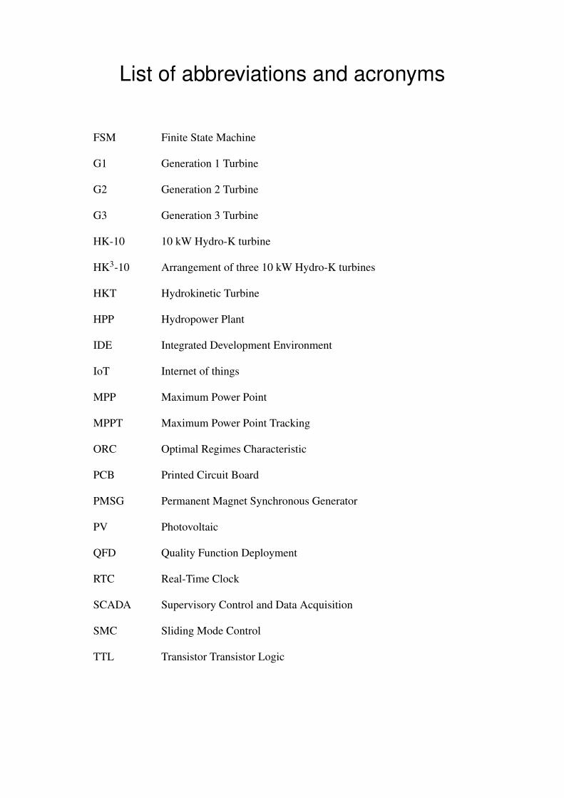
List of abbreviations and acronyms
FSM Finite State Machine
G1 Generation 1 Turbine
G2 Generation 2 Turbine
G3 Generation 3 Turbine
HK-10 10 kW Hydro-K turbine
HK3-10 Arrangement of three 10 kW Hydro-K turbines
HKT Hydrokinetic Turbine
HPP Hydropower Plant
IDE Integrated Development Environment
IoT Internet of things
MPP Maximum Power Point
MPPT Maximum Power Point Tracking
ORC Optimal Regimes Characteristic
PCB Printed Circuit Board
PMSG Permanent Magnet Synchronous Generator
PV Photovoltaic
QFD Quality Function Deployment
RTC Real-Time Clock
SCADA Supervisory Control and Data Acquisition
SMC Sliding Mode Control
TTL Transistor Transistor Logic

List of symbols
α Angular Acceleration rad/s2
λ Tip-speed Ratio dimensionless unit
ρ Density kg/m3
τ Torque N·m
ω Rotor Angular Velocity rad/s
A Rotor swept Area m2
CP Power Coefficient dimensionless unit
i Current A
I Inertia kg·m2
P Power W
R Resistance Ω
r Rotor radius m
t Time s
U Water velocity m/s
V Voltage V
Contents
1 INTRODUCTION . . . . . . . . . . . . . . . . . . . . . . . . . . . . . . . 16
2 HYDROKINETIC ENERGY CONVERTERS . . . . . . . . . . . . . . . . . 20
2.1 Classification of hydrokinetic energy converters . . . . . . . . . . . . 20
2.2 Comparing hydrokinetic energy converters with hydro power . . . . . 24
2.3 Hydrokinetic turbine control strategies . . . . . . . . . . . . . . . . . . 24
3 HISTORY AND TECHNOLOGICAL DEVELOPMENT OF HYDROKINETIC
TURBINES AT UNB . . . . . . . . . . . . . . . . . . . . . . . . . . . . . 27
3.1 First generation hydro-kinetic turbine (G1) . . . . . . . . . . . . . . . . 27
3.2 Second generation hydro-kinetic turbine (G2) . . . . . . . . . . . . . . 29
3.3 Third generation hydro-kinetic turbine (G3) . . . . . . . . . . . . . . . 30
3.4 Tucunaré hydro-kinetic turbine . . . . . . . . . . . . . . . . . . . . . . 31
3.5 Hydro-K project . . . . . . . . . . . . . . . . . . . . . . . . . . . . . . . 32
4 INSTRUMENTATION PLATFORM . . . . . . . . . . . . . . . . . . . . . . 35
4.1 Informational project . . . . . . . . . . . . . . . . . . . . . . . . . . . . 35
4.1.1 Stakeholder analysis . . . . . . . . . . . . . . . . . . . . . . . . . . . . . 35
4.1.2 Life cycle analysis . . . . . . . . . . . . . . . . . . . . . . . . . . . . . . 37
4.1.3 Client requirements . . . . . . . . . . . . . . . . . . . . . . . . . . . . . 37
4.1.4 Product requirements . . . . . . . . . . . . . . . . . . . . . . . . . . . . 41
4.2 Conceptual design . . . . . . . . . . . . . . . . . . . . . . . . . . . . . 44
4.2.1 Functional structure of the product . . . . . . . . . . . . . . . . . . . . . . 45
4.2.2 The search for alternative solutions and concepts . . . . . . . . . . . . . . 50
4.2.3 Product concept . . . . . . . . . . . . . . . . . . . . . . . . . . . . . . . 53
4.3 Detailed design . . . . . . . . . . . . . . . . . . . . . . . . . . . . . . . 59
4.3.1 Hardware . . . . . . . . . . . . . . . . . . . . . . . . . . . . . . . . . . . 59
4.3.2 Software development . . . . . . . . . . . . . . . . . . . . . . . . . . . . 64
4.4 Prototypes and tests . . . . . . . . . . . . . . . . . . . . . . . . . . . . 67
5 CONTROL OF HYDROKINETIC TURBINES . . . . . . . . . . . . . . . . 71
5.1 Non-MPPT variable speed - fixed pitch turbine control . . . . . . . . . 71
5.2 Maximum Power Point Tracking (MPPT) . . . . . . . . . . . . . . . . . 72

5.2.1 MPPT for PV systems . . . . . . . . . . . . . . . . . . . . . . . . . . . . 73
5.2.2 MPPT for wind energy systems . . . . . . . . . . . . . . . . . . . . . . . 74
5.2.3 MPPT for hydrokinetic turbines . . . . . . . . . . . . . . . . . . . . . . . . 75
5.3 Algorithm by ZHOU . . . . . . . . . . . . . . . . . . . . . . . . . . . . . 75
5.4 Algorithm by MOFEI . . . . . . . . . . . . . . . . . . . . . . . . . . . . 76
5.5 Proposed MPPT algorithm . . . . . . . . . . . . . . . . . . . . . . . . . 77
6 SIMULATION MODELING . . . . . . . . . . . . . . . . . . . . . . . . . . 79
6.1 Rotor modeling . . . . . . . . . . . . . . . . . . . . . . . . . . . . . . . 79
6.2 Gearbox modeling . . . . . . . . . . . . . . . . . . . . . . . . . . . . . 80
6.3 Generator modeling . . . . . . . . . . . . . . . . . . . . . . . . . . . . 81
6.4 Signal processing . . . . . . . . . . . . . . . . . . . . . . . . . . . . . . 82
6.5 Modeling of the MPPT algorithms . . . . . . . . . . . . . . . . . . . . . 83
6.6 Modeling of the optimal ω control . . . . . . . . . . . . . . . . . . . . . 85
7 RESULTS . . . . . . . . . . . . . . . . . . . . . . . . . . . . . . . . . . 89
7.1 Instrumentation results . . . . . . . . . . . . . . . . . . . . . . . . . . . 89
7.2 Simulation results . . . . . . . . . . . . . . . . . . . . . . . . . . . . . 93
8 CONCLUSIONS . . . . . . . . . . . . . . . . . . . . . . . . . . . . . . . 98
8.1 Instrumentation conclusions . . . . . . . . . . . . . . . . . . . . . . . 98
8.1.1 Future work . . . . . . . . . . . . . . . . . . . . . . . . . . . . . . . . . . 98
8.2 Simulation conclusions . . . . . . . . . . . . . . . . . . . . . . . . . . 99
8.2.1 Future research . . . . . . . . . . . . . . . . . . . . . . . . . . . . . . . 99
BIBLIOGRAPHY . . . . . . . . . . . . . . . . . . . . . . . . . . . . . . . 100
APPENDIX 104
APPENDIX A – SENSOR SELECTION MATRIX . . . . . . . . . . . . . . 105
APPENDIX B – PIN REFERENCE . . . . . . . . . . . . . . . . . . . . . 108
B.1 Instrumentation platform schematic . . . . . . . . . . . . . . . . . . . 110
APPENDIX C – PREVIOUS PROTOTYPES PCB . . . . . . . . . . . . . 113
APPENDIX D – LATEST PROTOTYPE PCB . . . . . . . . . . . . . . . . 115

APPENDIX E – CURRENT TRANSFORMER’S SIGNAL CONDITIONING
PCB . . . . . . . . . . . . . . . . . . . . . . . . . . . . 116
APPENDIX F – VOLTAGE DIVIDER PCB . . . . . . . . . . . . . . . . . 117
APPENDIX G – AMPLIFIER PCB . . . . . . . . . . . . . . . . . . . . . 118
APPENDIX H – ARDUINO CODE . . . . . . . . . . . . . . . . . . . . . 119
APPENDIX I – SENSOR CALIBRATION . . . . . . . . . . . . . . . . . 133
16
1 Introduction
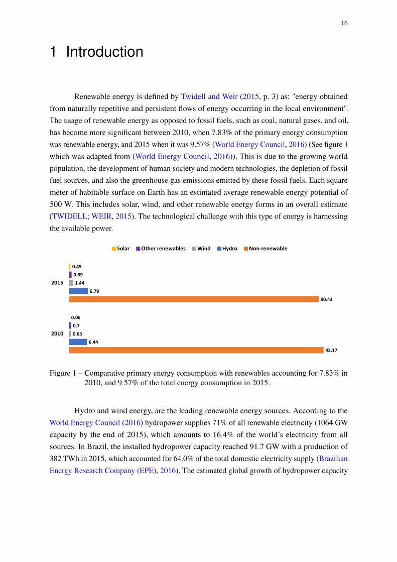
Renewable energy is defined by Twidell and Weir (2015, p. 3) as: "energy obtainedfrom naturally repetitive and persistent flows of energy occurring in the local environment".The usage of renewable energy as opposed to fossil fuels, such as coal, natural gases, and oil,has become more significant between 2010, when 7.83% of the primary energy consumptionwas renewable energy, and 2015 when it was 9.57% (World Energy Council, 2016) (See figure 1which was adapted from (World Energy Council, 2016)). This is due to the growing worldpopulation, the development of human society and modern technologies, the depletion of fossilfuel sources, and also the greenhouse gas emissions emitted by these fossil fuels. Each squaremeter of habitable surface on Earth has an estimated average renewable energy potential of500 W. This includes solar, wind, and other renewable energy forms in an overall estimate(TWIDELL; WEIR, 2015). The technological challenge with this type of energy is harnessingthe available power.
92.17
90.43
6.44
6.79
0.63
1.44
0.7
0.89
0.06
0.45
2010
2015
Solar Other renewables Wind Hydro Non-renewable
Figure 1 – Comparative primary energy consumption with renewables accounting for 7.83% in2010, and 9.57% of the total energy consumption in 2015.
Hydro and wind energy, are the leading renewable energy sources. According to theWorld Energy Council (2016) hydropower supplies 71% of all renewable electricity (1064 GWcapacity by the end of 2015), which amounts to 16.4% of the world’s electricity from allsources. In Brazil, the installed hydropower capacity reached 91.7 GW with a production of382 TWh in 2015, which accounted for 64.0% of the total domestic electricity supply (BrazilianEnergy Research Company (EPE), 2016). The estimated global growth of hydropower capacity

Chapter 1. Introduction 17
is around 29% by the year 2020. And the global wind energy reached around 435 GW capacityby the end of 2015. Wind and hydro power show great potential in competing with fossil energysources (World Energy Council, 2016).
After decades of research and development, solar and wind energy have already beendeployed all over the world. Marine and hydro-kinetic energy, such as wave energy, tidalcurrent, open-ocean current, river current, and thermal gradients in the ocean, are less common(THRESHER, 2011) and have a combined energy capacity of around 0.5 GW of which 99%is produced by tidal current energy (Ocean Energy Systems, 2015). This energy is harnessedusing hydrokinetic turbines (HKT) which convert the kinetic energy of free flowing water intoelectric energy. Information regarding estimations of riverflow energy potential for hydrokineticturbines is scarce. Nevertheless, flowing rivers are an energy source for hydrokinetic energyconverters.
Hydrokinetic turbines are hydrokinetic energy converters that harnesses energy from afree flowing current, i.e., no dams are needed. The efficiency of HKT’s are greatly impactedby two parts in particular: the rotor and the generator. The rotor converts the kinetic energyof the flowing water into a rotational torque that drives the generator, which in turn, produceselectricity. The problem with this system is that the point of optimal efficiency is dependent onthe fluctuating river velocity and the varying electrical load applied to the generator. Therefore,controlling a HKT in a wide range of velocity and load variation is a challenge (YUEN;APELFRÖJD; LEIJON, 2013).
A Brazilian project named Hydro-K started designing a fixed-pitch variant of such ariver flow HKT in cooperation with the University of Brasilia (UnB) in 2015. The researchpresented in this dissertation is part of this project. The author has contributed to this project inthe form of instrumentation and a control strategy for the HKT.
There are several control strategies for HKT’s. Most strategies involve rudimentarycontrol principles such as: load management, which regulates the load on a generator instead ofthe output of a generator; regulating the electromagnetic torque of a generator to manipulatethe generator output; adjusting the input torque of the generator mechanically, by for examplechanging the rotor-pitch angles or using a disc brake; and less common, controlling the kinetic-energy-carrying-fluid flow in order to adjust the energy available for harnessing.
A moderately researched control strategy for HKT’s is the "maximum power pointtracking" (MPPT) control. As the name suggests, it strives to find the maximum power, andmaintain the operating point at maximum power. This type of control has been more amplyresearched and implemented in wind turbines. An interesting property of this strategy is that

Chapter 1. Introduction 18
the generator voltage and current measurements are sufficient for estimating the generator’soperating point, while other strategies require some parameters to be mapped. The fact that thegenerator’s power output is used as a reference also means that the electrical output should beat it’s peak, because the peak electrical power does not occur at the peak mechanical power(AUBRÉE et al., 2016)
The first objective of this study will be to develop a MPPT algorithm to control theHydro-K HKT and thereby ensuring optimal energy harnessing from the riverflow. The inputsfor this algorithm should exclusively be the current and voltage generated by the generator,with the goal of maintaining the maximum generator output at various water velocities.
Keeping in mind that the turbine is experimental, there are a number of parameters thatwill be monitored for further research and development of the hydrokinetic turbine. Monitoringthese parameters remotely poses many challenges. An even greater challenge is creating aplatform capable of monitoring similar or future projects. Therefore, the second objective ofthis dissertation is the design of an instrumentation platform with flexibility at heart. Andthereby enabling the use of this platform for various types of turbines.
The methodology for assessing the functionality of the MPPT algorithm will be tofirstly do a literature review to identify MPPT algorithms and to identify the problems withthese existing algorithms. the HKT will at first be modeled and then the control algorithm canbe simulated to study the system’s behavior at varying river velocities. Next, an algorithm willbe created with a solution of the previously identified problems. To test the created algorithm, amodel of the hydrokinetic turbine with all of its components will be generated in "SIMULINK".Finally, the algorithm will be implemented in this model and compared with the differentalgorithms found in literature.
The methodology on which the design of the instrumentation platform is based isthe "product development process" developed by ROZENFELD et al., which includes fourmain development phases. The first phase is the informational design phase, here the designerattempts to acquire the customer’s needs. And through a process and several tools, the designercan formulate product specifications. The next step is the conceptual design phase, which isfocused on the use of the product specifications to generate alternative solutions and definethe architecture of the product. The following step, the detailed design, is a more technicalphase, where the necessary calculations and drawings are made for the last phase, which is theproduction and testing of prototypes. In the latter phase, prototypes are made to improve theproduct by testing its operation for the identification of unforeseen problems.
The contributions of this work to the academic community will be the comparison

Chapter 1. Introduction 19
of various MPPT algorithms and the availability of an instrumentation platform for variousapplications.
This dissertation is structured as follows: First off, the various hydrokinetic energyconverter technologies will be presented in chapter 2 to clarify which type of HKT will bestudied. Chapter 3 will discuss the history UnB has with hydrokinetic turbines and introducethe current Hydro-K project. Chapter 4 covers the design and fabrication of the instrumentationplatform which will monitor the turbine’s functionality. Next, chapter 5 will review the controlof hydrokinetic turbines and MPPT in more detail. Chapter 6 will explain the simulation models.And finally, chapters 7 and 8 will discuss the results and conclusions.

20
2 Hydrokinetic energy converters
2.1 Classification of hydrokinetic energy converters
Hydrokinetic energy converters harvest kinetic energy from flowing water and convertthis energy directly into electricity without the need of elevated water reservoirs commonlyknown as dams. This is why they are also called free flow turbines, ultra-low- or zero-head-hydro turbines. Sources of hydrokinetic energy range from natural flowing rivers, tidal estuaries,ocean currents, and waves, to various man-made waterways.
Hydrokinetic energy technology has been developing in the last 2 decades and is one ofthe fastest growing renewable energy technology (Ocean Renewable Energy Coalition (OREC);Verdant Power, 2012). The majority of the hydrokinetic energy converter systems are in theresearch and development phase, and a small group is in the pre-commercial phase (KHAN;BHUYAN, 2009). There are more than 100 conceptual designs of hydrokinetic energy convertersystems (COPPING et al., 2013)(EDENHOFER et al., 2011).
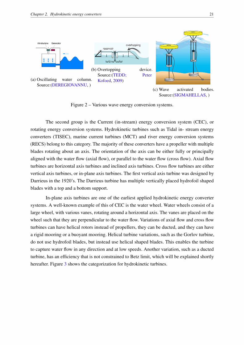
Hydrokinetic energy converters are classified in two main groups (YUCE; MURATOGLU,2015). The first group is the Wave Energy Conversion (WEC) systems. As the name suggests,these systems utilize the movements and kinetic energy originating from waves. These systemsvary in size, orientation, and distance from the shore, and can be divided into three main subcategories, namely, Oscillating Water Columns (OWC), Over Topping Devices (OTD), andWave Activated Bodies (WAB). As WEC’s are not within the scope of this work, they will notbe discussed in detail, but figure 2 illustrates the main working principles. Figure 2a showsan OWC which rotates an air turbine using the suction and overpressure caused by waves.Figure 2b shows an OTD which drives a turbine with water entering a reservoir due to waves.And lastly, figure 2c shows a WAB, which hydraulically pumps water through a turbine, as abuoy moves with the waves.
Chapter 2. Hydrokinetic energy converters 21
(a) Oscillating water column.Source:(DEREGIOVANNU, )
(b) Overtopping device.Source:(TEDD; PeterKofoed, 2009)
(c) Wave activated bodies.Source:(SIGMAHELLAS, )
Figure 2 – Various wave energy conversion systems.
The second group is the Current (in-stream) energy conversion system (CEC), orrotating energy conversion systems. Hydrokinetic turbines such as Tidal in- stream energyconverters (TISEC), marine current turbines (MCT) and river energy conversion systems(RECS) belong to this category. The majority of these converters have a propeller with multipleblades rotating about an axis. The orientation of the axis can be either fully or principallyaligned with the water flow (axial flow), or parallel to the water flow (cross flow). Axial flowturbines are horizontal axis turbines and inclined axis turbines. Cross flow turbines are eithervertical axis turbines, or in-plane axis turbines. The first vertical axis turbine was designed byDarrieus in the 1920’s. The Darrieus turbine has multiple vertically placed hydrofoil shapedblades with a top and a bottom support.
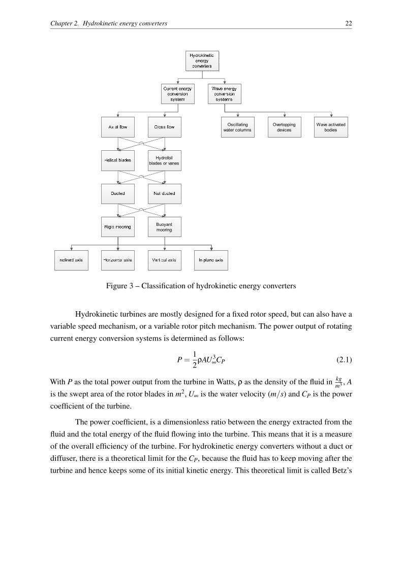
In-plane axis turbines are one of the earliest applied hydrokinetic energy convertersystems. A well-known example of this of CEC is the water wheel. Water wheels consist of alarge wheel, with various vanes, rotating around a horizontal axis. The vanes are placed on thewheel such that they are perpendicular to the water flow. Variations of axial flow and cross flowturbines can have helical rotors instead of propellers, they can be ducted, and they can havea rigid mooring or a buoyant mooring. Helical turbine variations, such as the Gorlov turbine,do not use hydrofoil blades, but instead use helical shaped blades. This enables the turbineto capture water flow in any direction and at low speeds. Another variation, such as a ductedturbine, has an efficiency that is not constrained to Betz limit, which will be explained shortlyhereafter. Figure 3 shows the categorization for hydrokinetic turbines.
Chapter 2. Hydrokinetic energy converters 22
Oscillating
water columns
Overtopping
devices
Wave activated
bodies
Hydrofoil
blades or vanes
Buoyant
mooring
Figure 3 – Classification of hydrokinetic energy converters
Hydrokinetic turbines are mostly designed for a fixed rotor speed, but can also have avariable speed mechanism, or a variable rotor pitch mechanism. The power output of rotatingcurrent energy conversion systems is determined as follows:
P =12
ρAU3∞CP (2.1)
With P as the total power output from the turbine in Watts, ρ as the density of the fluid in kgm3 , A
is the swept area of the rotor blades in m2, U∞ is the water velocity (m/s) and CP is the powercoefficient of the turbine.
The power coefficient, is a dimensionless ratio between the energy extracted from thefluid and the total energy of the fluid flowing into the turbine. This means that it is a measureof the overall efficiency of the turbine. For hydrokinetic energy converters without a duct ordiffuser, there is a theoretical limit for the CP, because the fluid has to keep moving after theturbine and hence keeps some of its initial kinetic energy. This theoretical limit is called Betz’s
Chapter 2. Hydrokinetic energy converters 23
coefficient of performance or Betz limit and is described as (BETZ, 1920):
CpB =1627
= 0.593 (2.2)
This means that unducted turbines have a maximum theoretical efficiency of 59.3%. Theefficiency of hydrokinetic turbines can also be given in CP
CpB, which is the efficiency of the
turbine relative to its maximum theoretical efficiency.
The power coefficient can be calculated as follows:
CP =P
0.5ρAU3∞
(2.3)
Where P is the total power output from the turbine in Watts, ρ is the density of the fluid in kgm3 ,
A is the swept area of the rotor blades in m2, and U∞ is the water velocity in ms . Hydrokinetic
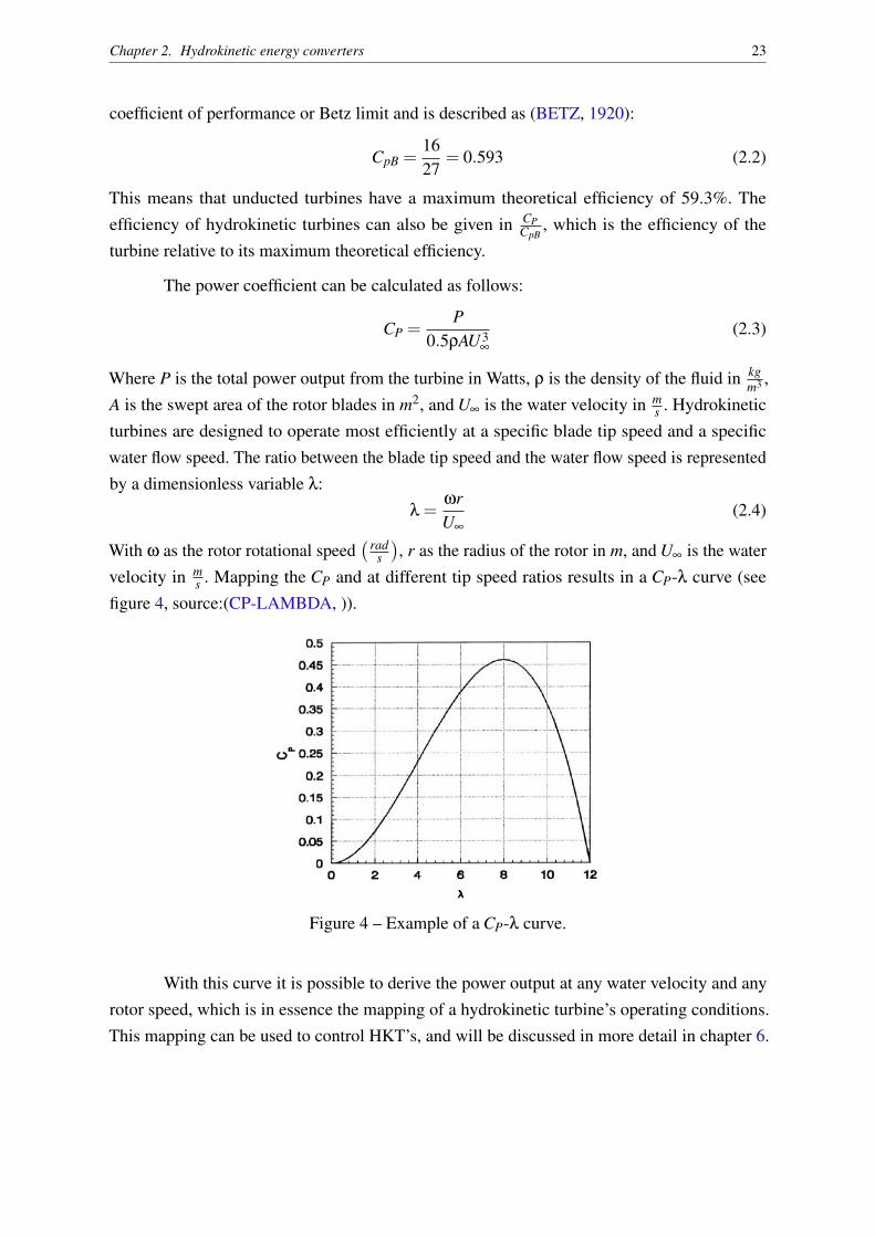
turbines are designed to operate most efficiently at a specific blade tip speed and a specificwater flow speed. The ratio between the blade tip speed and the water flow speed is representedby a dimensionless variable λ:
λ =ωrU∞
(2.4)
With ω as the rotor rotational speed( rad
s
), r as the radius of the rotor in m, and U∞ is the water
velocity in ms . Mapping the CP and at different tip speed ratios results in a CP-λ curve (see
figure 4, source:(CP-LAMBDA, )).
Figure 4 – Example of a CP-λ curve.
With this curve it is possible to derive the power output at any water velocity and anyrotor speed, which is in essence the mapping of a hydrokinetic turbine’s operating conditions.This mapping can be used to control HKT’s, and will be discussed in more detail in chapter 6.

Chapter 2. Hydrokinetic energy converters 24
2.2 Comparing hydrokinetic energy converters with hydro power
It is the author’s experience that hydrokinetic energy converters are often overlookedas sources of electricity, and that one tends to opt for hydro power instead of HKT’s. In thecase of large scale power generation, hydro power has the clear advantage, but in small scale,hydrokinetic energy converters can be more convenient. And by combining both technologies,one can increase the efficiency of hydro power plants by harnessing the residual kineticenergy at the plant’s outlet, which is exactly the case for the Hydro-K project. To advocate theconsideration of using hydrokinetic energy converters, this section is dedicated to comparingthe advantages and disadvantages of hydrokinetic energy converters.
First of all, hydrokinetic energy converters require very little civil work compared todams, but only generate power on a small scale. Eventhough hydrokinetic energy converterscan be installed in–wind farm like–multi-unit arrays, they have a lower efficiency of barely35%, compared to the 80-90% efficiency of hydro power plants. The energy predictability ofhydrokinetic turbines is similar to that of hydro power plants, and both hinder navigation andfishery in their installed areas, but hydrokinetic turbines have the advantage of having a largerrange of applicability, for example, they can be installed in remote- off-grid areas, in areas withseismic hazards, and in highly populated areas. Above all, hydrokinetic turbines have muchless environmental effects, and eventhough the electric energy cost of this technology is high,the development of the technology will increase its efficiency, and will most likely render it amajor source of cost effective electricity by 2050 (MAGANA et al., 2014).
The lower environmental effects of hydrokinetic turbines include evading: the relocationof people, the inundation of agriculture, historical sites and animal habitats, the sedimentationof fertile lands, the production of methane due to submerged vegetation, and the alteration ofriver regimes. Although it’s obvious environmental advantages, this technology can still affectthe environment due to its parts, the chemical agents, and the noise and vibrations of the turbinecan also affect the water habitat.
2.3 Hydrokinetic turbine control strategies
Tidal turbines are subject to forecasted tide conditions. River turbines on the other handmay not be dependent on tide conditions. River turbines downstream of Hydro Power Plants(HPP) are strongly dependent on the plant’s output flow, be it through spillgates and/or turbineoutlets. The prediction of tidal conditions is somewhat straightforward, as readily available tide
Chapter 2. Hydrokinetic energy converters 25
tables are available and have shown a 98% accuracy for decades. These tables can be used incoordinating the tidal plant’s operation (ZHOU et al., 2014). Depending on the configuration ofthe HPP, the resource for river turbines downstream of HPP’s, can be less predictable due tofluctuations in power demand. However, the advantages for this HPP-river turbine configurationare that the majority of HPP’s monitor the plant’s output flow, and this flow tends to changemore gradually. Using the plant’s output flow data and the site’s bathymetry, a correlationbetween the plant’s output flow and the river velocity can be made. This correlation could thenbe used to coordinate the operation of the river turbine. The cases described above have morepredictable resources, contrary to wind turbines.
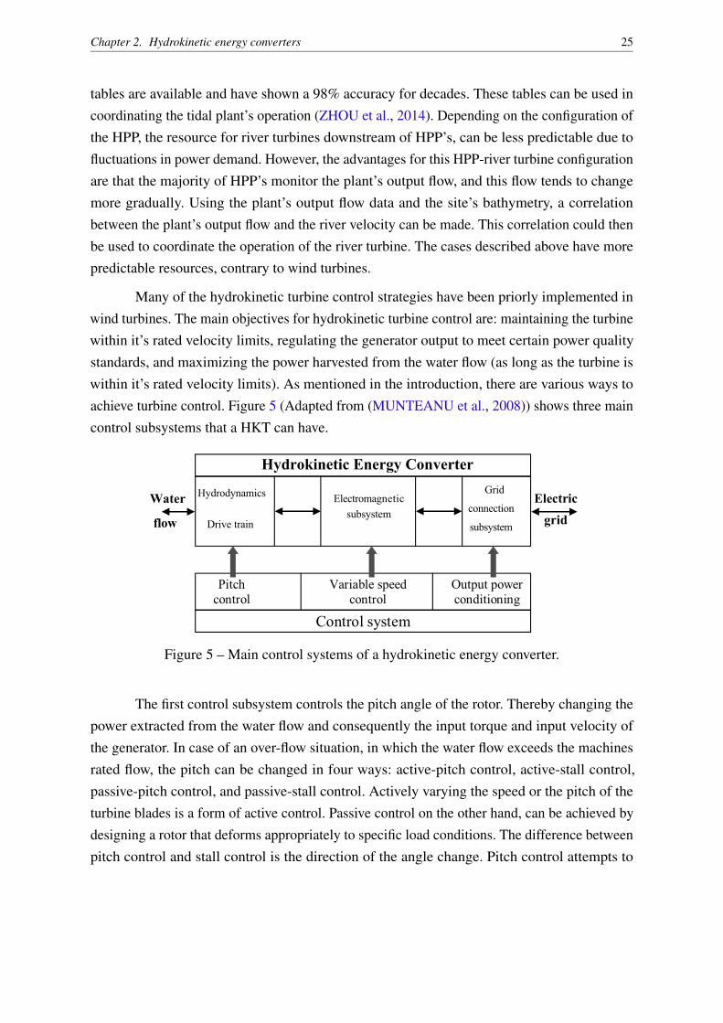
Many of the hydrokinetic turbine control strategies have been priorly implemented inwind turbines. The main objectives for hydrokinetic turbine control are: maintaining the turbinewithin it’s rated velocity limits, regulating the generator output to meet certain power qualitystandards, and maximizing the power harvested from the water flow (as long as the turbine iswithin it’s rated velocity limits). As mentioned in the introduction, there are various ways toachieve turbine control. Figure 5 (Adapted from (MUNTEANU et al., 2008)) shows three maincontrol subsystems that a HKT can have.
4
Basics of the Wind Turbine Control Systems
4.1 Control Objectives
Taking into account the ideas presented in the previous chapters, one can highlight the objectives of the WECS control (see Section 2.7). The list bellow selects the most important:
controlling the wind captured power for speeds larger than the rated; maximising the wind harvested power in partial load zone as long as constraints on speed and captured power are met; alleviating the variable loads, in order to guarantee a certain level of resilience of the mechanical parts; meeting strict power quality standards (power factor, harmonics, flicker, etc.);transferring the electrical power to the grid at an imposed level, for wide range
Hydrodynamics Electromagnetic subsystem
Grid
connection
subsystemDrive train
Water
flow
Electric grid
Pitchcontrol
Variable speedcontrol
Output power conditioning
Hydrokinetic Energy Converter
Control system
The first control subsystem affects the pitch angle following aerodynamic power limiting targets. The second implements the generator control, in order to
Figure 5 – Main control systems of a hydrokinetic energy converter.
The first control subsystem controls the pitch angle of the rotor. Thereby changing thepower extracted from the water flow and consequently the input torque and input velocity ofthe generator. In case of an over-flow situation, in which the water flow exceeds the machinesrated flow, the pitch can be changed in four ways: active-pitch control, active-stall control,passive-pitch control, and passive-stall control. Actively varying the speed or the pitch of theturbine blades is a form of active control. Passive control on the other hand, can be achieved bydesigning a rotor that deforms appropriately to specific load conditions. The difference betweenpitch control and stall control is the direction of the angle change. Pitch control attempts to

Chapter 2. Hydrokinetic energy converters 26
angle the leading edge of the blade towards the incoming flow. Stall control is also known asnegative pitch control, and directs the leading edge of the blade away from the incoming flow.(MOTLEY; BARBER, 2014) examined the possibilities of passive pitch adaption for marinehydrokinetic turbines.
The second control subsystem manages the generator in order to obtain a variable speedregime. Traditional horizontal axis turbines fall into one of four categories: fixed speed - fixedpitch, variable speed - fixed pitch, fixed speed - variable pitch, or variable speed - variablepitch. For each water velocity, there is a certain rotational speed at which the power curve of ahydrokinetic turbine reaches a maximum. The curve described by connecting all the maxima ofdifferent water velocities is known as the Optimal Regimes Characteristic (ORC). The Variablespeed control system aims to keep the generator velocity at the velocity corresponding to thismaximum.
The last control subsystem, which is "output power conditioning", smoothens thetransfer of the generator output electric power to the electric load. The smoothing can beachieved by adding capacitor banks or other power electronics devices. Adding these devicesimplies a supplementary power loss, but they favor generator motion control, which allows thepositioning of the operation point on the ORC.
Considering the theme of this dissertation, chapter 5 is dedicated to discuss the optimalcontrol approaches of variable speed - fixed pitch turbines.

27
3 History and technological development of
hydrokinetic turbines at UnB
3.1 First generation hydro-kinetic turbine (G1)
The first recorded Brazilian experience with hydrokinetic turbines (HKT) was in 1981,when Harwood and Almeida tested a HKT in the amazonian "Solimões River" (HARWOOD,1985). Research on HKT’s started at UnB when a research group of the Mechanical EngineeringDepartment tested various prototypes, and installed the first operational HKT in 1995 at a riverlocated near the city Correntina in the state of Bahia. This HKT was named "Generation 1"and with it’s 1 kW capacity, provided electricity to a nearby medical post. Generation 1 wastested with various axial-rotors with 2 blades, 6 blades, and 18 blades. The axial-6-bladed rotorwith a diameter of 0.8 m proved to be the most efficient of the tested rotors (ELS et al., 2003).The rotor was protected from large and potentially harmful debris by a conical steel grid asshown in figure 6 (Brasil Jr. et al., 2007). Furthermore, the turbine had a stator which guidedthe entering water flow into the rotor. The HKT had a brushed AC generator with a manuallyvariable stator excitation and an overvoltage protection system based on a 1 kW thyristor drivenload (see figure 7).
Figure 6 – Generation 1 turbine source: Els et al. (2003).
Chapter 3. History and technological development of hydrokinetic turbines at UnB 28
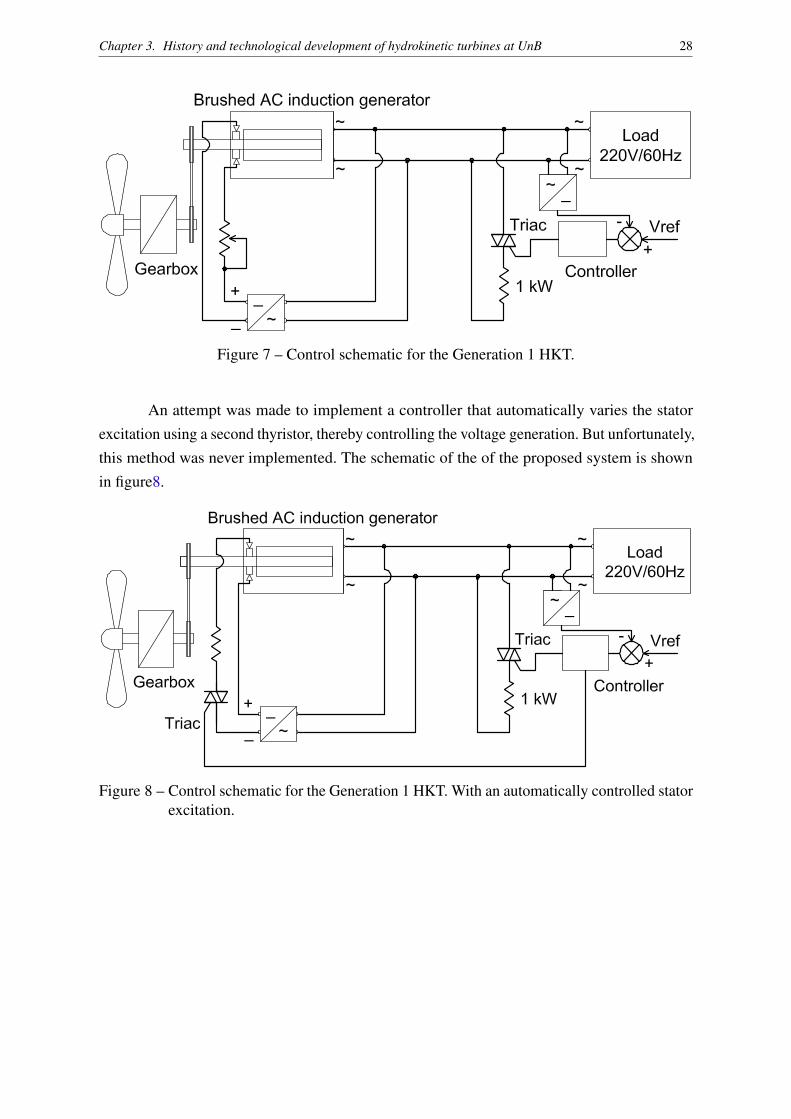
Figure 7 – Control schematic for the Generation 1 HKT.
An attempt was made to implement a controller that automatically varies the statorexcitation using a second thyristor, thereby controlling the voltage generation. But unfortunately,this method was never implemented. The schematic of the of the proposed system is shownin figure8.
Figure 8 – Control schematic for the Generation 1 HKT. With an automatically controlled statorexcitation.
Chapter 3. History and technological development of hydrokinetic turbines at UnB 29
3.2 Second generation hydro-kinetic turbine (G2)
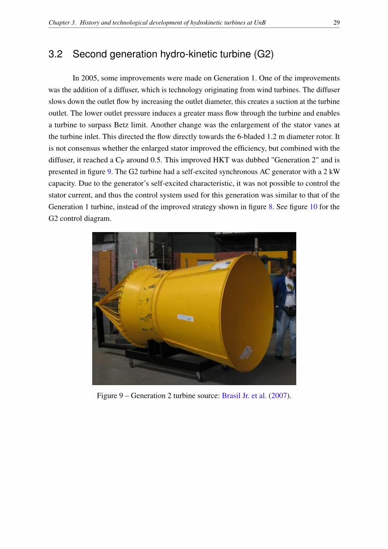
In 2005, some improvements were made on Generation 1. One of the improvementswas the addition of a diffuser, which is technology originating from wind turbines. The diffuserslows down the outlet flow by increasing the outlet diameter, this creates a suction at the turbineoutlet. The lower outlet pressure induces a greater mass flow through the turbine and enablesa turbine to surpass Betz limit. Another change was the enlargement of the stator vanes atthe turbine inlet. This directed the flow directly towards the 6-bladed 1.2 m diameter rotor. Itis not consensus whether the enlarged stator improved the efficiency, but combined with thediffuser, it reached a CP around 0.5. This improved HKT was dubbed "Generation 2" and ispresented in figure 9. The G2 turbine had a self-excited synchronous AC generator with a 2 kWcapacity. Due to the generator’s self-excited characteristic, it was not possible to control thestator current, and thus the control system used for this generation was similar to that of theGeneration 1 turbine, instead of the improved strategy shown in figure 8. See figure 10 for theG2 control diagram.Capítulo 1. Introdução 3
Figura 2 – Foto da turbina hidrocinética Geração 2.
Fonte: Brasil et al. (2007)
transmissão entre o rotor e o gerador diminuam; um novo difusor. A geometria dessedifusor era inovadora, pois ele não era um difusor cônico e sim achatado. Essa característicafoi dada pensando no posicionamento da turbina no rio, sendo que essa nova geometriaexige um rio menos profundo. Outra inovação no difusor, foi uma abertura, após a turbina,que permitia que o escoamento externo passe dentro do difusor, contribuindo para evitardescolamentos de camada limite na parede do difusor e diminuindo efeitos de recirculação.A Geração 3 obteve um Cp de aproximadamente 1,0 em suas simulações numéricas eem ensaio de modelo reduzido na escala de 1:10 (SOUZA; OLIVEIRA; JUNIOR, 2006;BRASIL et al., 2007).
Carcaça
Difusor
Rotor 4 pás
Anel
Núcleo conversor
Figura 3 – Modelo geométrio da turbina hidrocinética Geração 3.
Fonte: Souza, Oliveira e Junior (2006, p. 32)
Figure 9 – Generation 2 turbine source: Brasil Jr. et al. (2007).
Chapter 3. History and technological development of hydrokinetic turbines at UnB 30
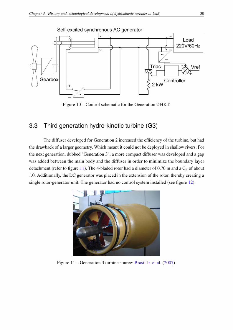
Figure 10 – Control schematic for the Generation 2 HKT.
3.3 Third generation hydro-kinetic turbine (G3)
The diffuser developed for Generation 2 increased the efficiency of the turbine, but hadthe drawback of a larger geometry. Which meant it could not be deployed in shallow rivers. Forthe next generation, dubbed "Generation 3", a more compact diffuser was developed and a gapwas added between the main body and the diffuser in order to minimize the boundary layerdetachment (refer to figure 11). The 4-bladed rotor had a diameter of 0.70 m and a CP of about1.0. Additionally, the DC generator was placed in the extension of the rotor, thereby creating asingle rotor-generator unit. The generator had no control system installed (see figure 12).
6
• Anel: O anel metálico que suporta o núcleo da máquina na carcaça; Este anel foi fundido em a-lumínio ordinário.
Uma imagem geral da vista explodida da turbina é apre-
sentada na figura 11, e uma foto geral do protótipo é mos-trado na figura 12.
Figura 11. Vista explodida do protótipo da turbina G3
Figura 12. Foto do protótipo Os ensaios do protótipo foram realizados de maneira e-
quivalente aos ensaios em modelo reduzido. No entanto, uma única velocidade de corrente foi utilizada (~1 m/s). O ensaio foi efetuado nem um canal artificial de profundidade de 1,5 m com largura de 4 m. O protótipo da turbina foi localizado no centro do canal. O gerador foi submetido à diferentes cargas resistivas, providas por um reostato. A velocidade do rio foi medida por um molinete calibrado e a rotação da máquina foi obtida por um sensor capacitivo ins-talada no núcleo da máquina, que transmitia em tempo real a rotação do eixo. Para diferentes cargas resistivas da máqui-na, foi mensuradas a potência gerada pelo gerador e sua rotação. Desta maneira a curva de potência pode ser obtida. Tal curva é apresentada na figura 13. Observa-se que os valores obtidos foram compatíveis com as previsões numé-ricas e de ensaio em túnel de vento.
0,0
0,2
0,4
0,6
0,8
1,0
4,60 4,70 4,80 4,90 5,00
λ
Cp
Figura 13. Ensaio do protótipo – Coeficiente de potência
IV. COMUNIDADES ISOLADAS E AS TURBINAS HIDROCINÉTI-CAS
A. Comunidade isoladas O conceito de comunidades remotas assumido aqui
considera um assentamento humano de baixa densidade populacional, com restrições ao uso de fontes de energia convencionais (sem acesso a linhas de energia com geração centralizada), com infra-estrutura urbana deficiente, com baixo nível de atividade econômica, com difícil acesso e distante de mercados consumidores.Evidentemente tais pa-râmetros são pouco específicos para uma caracterização precisa de uma comunidade remota. Esta é uma definição aberta que, no entanto, torna-se operacional quando a co-munidade deve ser encaixada em um planejamento de dis-ponibilização de energia. Em geral, comunidades remotas não viabilizam implantações de sistemas de provimento de energia elétrica no senso econômico estrito, utilizando uni-camente como parâmetros de análise investimento, demanda e receita.
Na Amazônia, diversos assentamentos humanos podem ser caracterizados como comunidades remotas. Várias co-munidades se estabeleceram fora da sede dos municípios, muitas vezes distanciadas de eixos rodoviários. Algumas comunidades foram estabelecidas em ilhas (e. g. Arquipéla-go do Marajó) e muitas foram construídas a partir de assen-tamentos de reforma agrária as vezes com difícil acesso. Comunidades estabelecidas em reservas extrativistas ou ainda as comunidades indígenas da região enquadram-se na caracterização de comunidades remotas.
O problema de disponibilização da energia para tais co-munidades é sempre um ponto crítico na implantação de infraestrutura mínima para a população isolada. Políticas públicas municipais em geral privilegiam investimentos de infra-estrutura na cidade sede do município. O problema da geração de energia em outras comunidades menores é sem-pre penalizado visto o baixo retorno de investimento e pela dificuldade de cobrança do uso da energia. A viabilidade deve ser vista considerando-se parâmetros mais amplos, objetivando assim a promoção do desenvolvimento susten-
Figure 11 – Generation 3 turbine source: Brasil Jr. et al. (2007).
Chapter 3. History and technological development of hydrokinetic turbines at UnB 31
Figure 12 – Control schematic for the Generation 3 HKT.
3.4 Tucunaré hydro-kinetic turbine
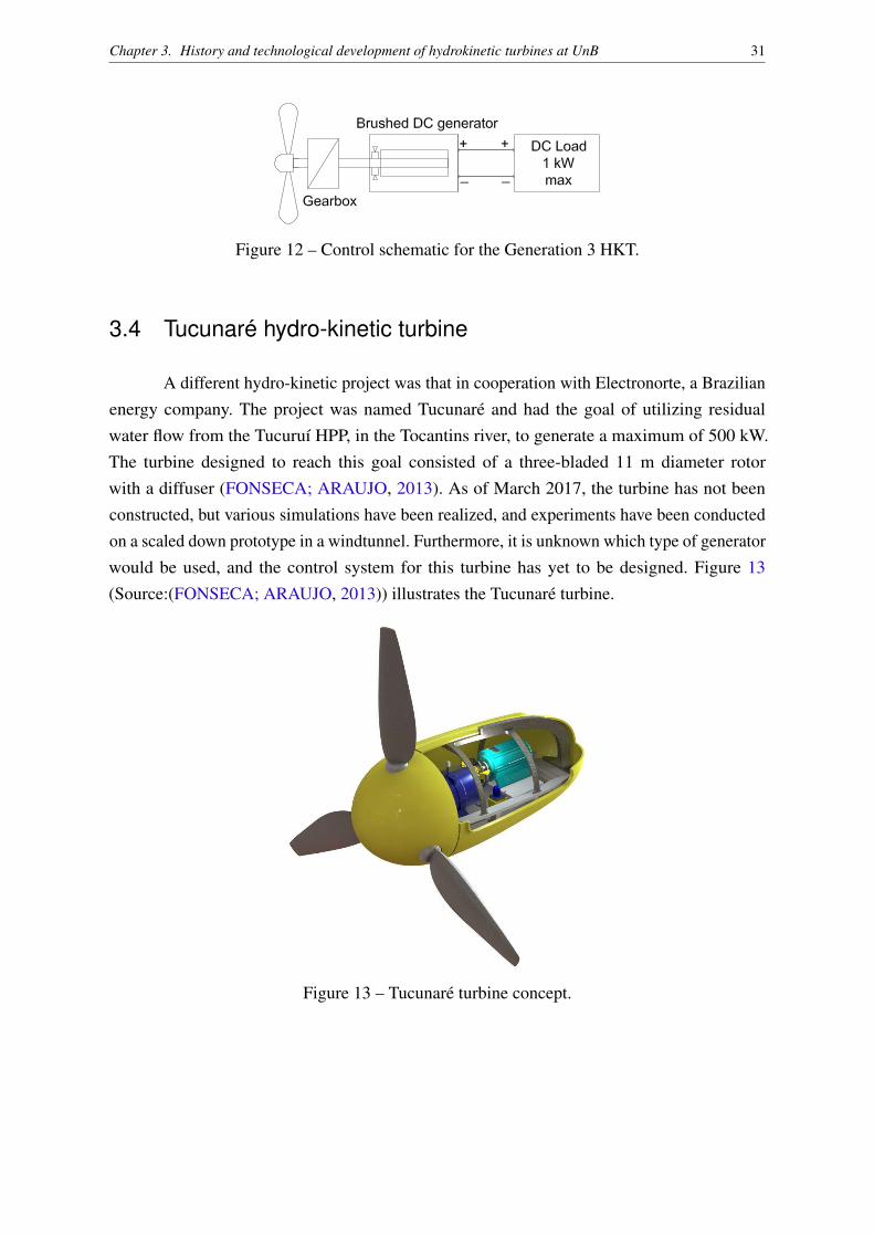
A different hydro-kinetic project was that in cooperation with Electronorte, a Brazilianenergy company. The project was named Tucunaré and had the goal of utilizing residualwater flow from the Tucuruí HPP, in the Tocantins river, to generate a maximum of 500 kW.The turbine designed to reach this goal consisted of a three-bladed 11 m diameter rotorwith a diffuser (FONSECA; ARAUJO, 2013). As of March 2017, the turbine has not beenconstructed, but various simulations have been realized, and experiments have been conductedon a scaled down prototype in a windtunnel. Furthermore, it is unknown which type of generatorwould be used, and the control system for this turbine has yet to be designed. Figure 13(Source:(FONSECA; ARAUJO, 2013)) illustrates the Tucunaré turbine.
Figure 13 – Tucunaré turbine concept.
Chapter 3. History and technological development of hydrokinetic turbines at UnB 32
3.5 Hydro-K project
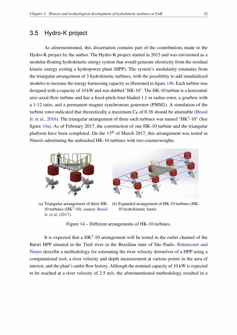
As aforementioned, this dissertation contains part of the contributions made to theHydro-K project by the author. The Hydro-K project started in 2015 and was envisioned as amodular-floating hydrokinetic energy system that would generate electricity from the residualkinetic energy exiting a hydropower plant (HPP). The system’s modularity emanates fromthe triangular arrangement of 3 hydrokinetic turbines, with the possibility to add standardizedmodules to increase the energy harnessing capacity as illustrated in figure 14b. Each turbine wasdesigned with a capacity of 10 kW and was dubbed "HK-10". The HK-10 turbine is a horizontal-axis-axial-flow turbine and has a fixed-pitch-four-bladed 1.1 m radius rotor, a gearbox witha 1:12 ratio, and a permanent magnet synchronous generator (PMSG). A simulation of theturbine rotor indicated that theoretically a maximum CP of 0.38 should be attainable (BrasilJr. et al., 2016). The triangular arrangement of three such turbines was named "HK3-10" (Seefigure 14a). As of February 2017, the construction of one HK-10 turbine and the triangularplatform have been completed. On the 13th of March 2017, this arrangement was tested inNiterói substituting the unfinished HK-10 turbines with two counterweights.
(a) Triangular arrangement of three HK-10 turbines (HK3-10). source: BrasilJr. et al. (2017).
(b) Expanded arrangement of HK-10 turbines (HK-10 hydrokinetic farm).
Figure 14 – Different arrangements of HK-10 turbines.
It is expected that a HK3-10 arrangement will be tested in the outlet channel of theBariri HPP situated in the Tietê river in the Brazilian state of São Paulo. Bittencourt andNunes describe a methodology for estimating the river velocity downriver of a HPP using acomputational tool, a river velocity and depth measurement at various points in the area ofinterest, and the plant’s outlet flow history. Although the nominal capacity of 10 kW is expectedto be reached at a river velocity of 2.5 m/s, the aforementioned methodology resulted in a
Chapter 3. History and technological development of hydrokinetic turbines at UnB 33
simulated river velocity, at the Bariri HPP, in the range of 0.61 m/s to 2.05 m/s (BITTENCOURT;NUNES, 2016).
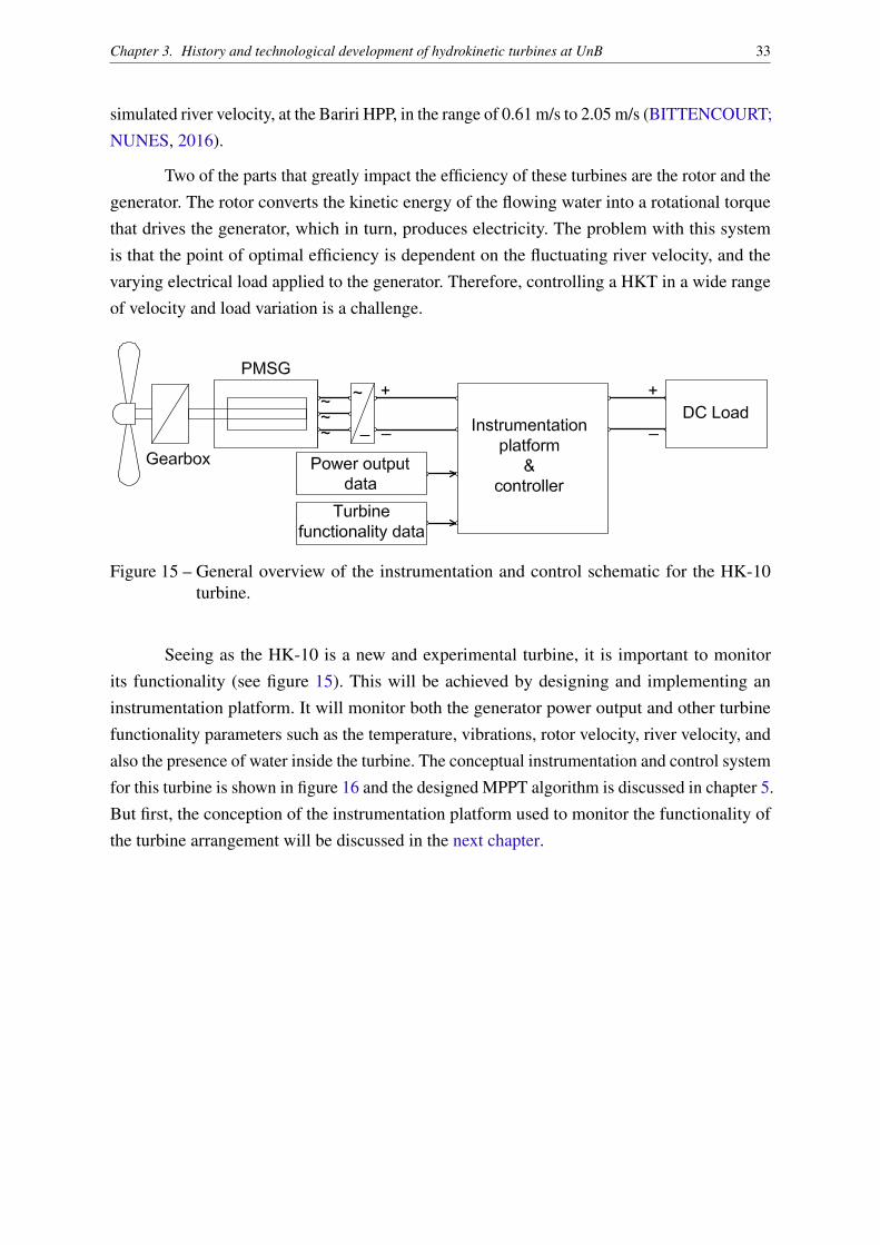
Two of the parts that greatly impact the efficiency of these turbines are the rotor and thegenerator. The rotor converts the kinetic energy of the flowing water into a rotational torquethat drives the generator, which in turn, produces electricity. The problem with this systemis that the point of optimal efficiency is dependent on the fluctuating river velocity, and thevarying electrical load applied to the generator. Therefore, controlling a HKT in a wide rangeof velocity and load variation is a challenge.
Figure 15 – General overview of the instrumentation and control schematic for the HK-10turbine.
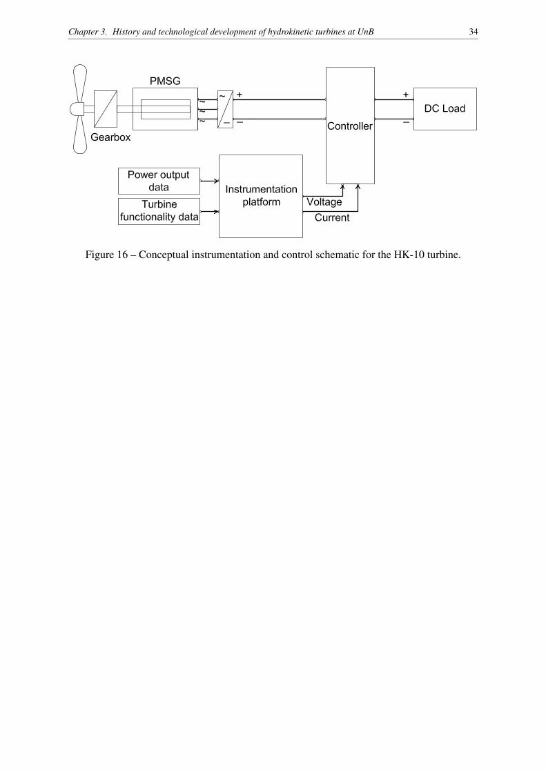
Seeing as the HK-10 is a new and experimental turbine, it is important to monitorits functionality (see figure 15). This will be achieved by designing and implementing aninstrumentation platform. It will monitor both the generator power output and other turbinefunctionality parameters such as the temperature, vibrations, rotor velocity, river velocity, andalso the presence of water inside the turbine. The conceptual instrumentation and control systemfor this turbine is shown in figure 16 and the designed MPPT algorithm is discussed in chapter 5.But first, the conception of the instrumentation platform used to monitor the functionality ofthe turbine arrangement will be discussed in the next chapter.
Chapter 3. History and technological development of hydrokinetic turbines at UnB 34
Figure 16 – Conceptual instrumentation and control schematic for the HK-10 turbine.
35
4 Instrumentation platform
An instrumentation platform was designed for hydrokinetic turbine monitoring appli-cations with specifically the HK-10 turbine in mind. This platform is a base on which otherinstrumentation applications can be realized, because reconfigurability was one of the mainobjectives in its design. Instrumentation for wind turbines, and hydrokinetic turbine- or windturbine windtunnel testing applications have many similar instrumentation requirements. Oneof those similarities is that the phenomenon under study is, when compared to electrical phe-nomenon, slow. Also, many of the individual measurement requirements are similar. Therefore,this instrumentation platform is focused on these three applications, but it is not limited to theseapplications.
4.1 Informational project
The primary goal of this platform is to facilitate research on wind- and hydrokinetic-turbines with the HK-10 turbines as a specific application, and secondarily incorporating flexi-bility for diverse instrumentation applications. One of the main reasons why the developmentof an instrumentation platform was chosen over the purchase of one, is the high cost of suchproducts. With that being said, another secondary goal is to minimize the cost of this product.The following sections will discuss its development.
4.1.1 Stakeholder analysis
A survey of stakeholders is required to get more details on the project requirements asthe product goes through its life cycle. By means of this survey, exhaustive product specificationlist can be generated.
The globally identified stakeholders for this project are listed below:
• Investors: the investors of this project are AES (Applied Energy Services), which is theBrazilian company funding the Hydro-K project, and UnB, which has produced varioushydrokinetic turbines and is stimulating its research.• Consumers: the consumers vary from a hobbyist to a research facility such as UnB.
Chapter 4. Instrumentation platform 36
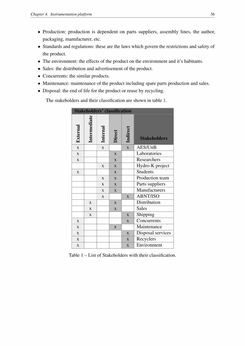
• Production: production is dependent on parts suppliers, assembly lines, the author,packaging, manufacturer, etc.• Standards and regulations: these are the laws which govern the restrictions and safety of
the product.• The environment: the effects of the product on the environment and it’s habitants.• Sales: the distribution and advertisement of the product.• Concurrents: the similar products.• Maintenance: maintenance of the product including spare parts production and sales.• Disposal: the end of life for the product or reuse by recycling.
The stakeholders and their classification are shown in table 1.
Stakeholders’ classification
Ext
erna
l
Inte
rmed
iate
Inte
r nal
Dir
ect
Indi
r ect
Stakeholders
x x x AES/UnBx x Laboratoriesx x Researchers
x x Hydro-K projectx x Students
x x Production teamx x Parts suppliersx x Manufacturersx x ABNT/ISO
x x Distributionx x Salesx x Shipping
x x Concurrentsx x Maintenancex x Disposal servicesx x Recyclersx x Environment
Table 1 – List of Stakeholders with their classification.
Chapter 4. Instrumentation platform 37
4.1.2 Life cycle analysis
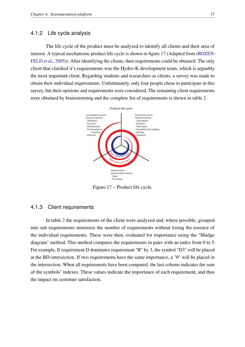
The life cycle of the product must be analyzed to identify all clients and their area ofinterest. A typical mechatronic product life cycle is shown in figure 17 (Adapted from (ROZEN-FELD et al., 2005)). After identifying the clients, their requirements could be obtained. The onlyclient that clarified it’s requirements was the Hydro-K development team, which is arguablythe most important client. Regarding students and researchers as clients, a survey was made toobtain their individual requirements. Unfortunately, only four people chose to participate in thissurvey, but their opinions and requirements were considered. The remaining client requirementswere obtained by brainstorming and the complete list of requirements is shown in table 2.
Production sector
(Internal clients):
- Conceptual
- Detailed
- Fabrication
- Assembly and Labeling
- Storage
- Transport
Market sector
(Intermediate clients):
- Sales
- Purchases
Consumption sector
(External clients):
- Utilization
- Function
- Maintenance
- Deactivation or
recycling
- Disposal
Product life cycle
Figure 17 – Product life cycle.
4.1.3 Client requirements
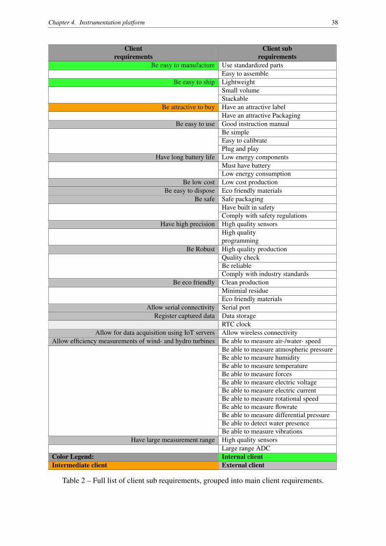
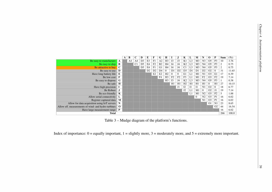
In table 2 the requirements of the client were analyzed and, where possible, groupedinto sub requirements minimize the number of requirements without losing the essence ofthe individual requirements. These were then, evaluated for importance using the "Mudgediagram" method. This method compares the requirements in pairs with an index from 0 to 5.For example, If requirement D dominates requirement "B" by 3, the symbol "D3" will be placedat the BD-intersection. If two requirements have the same importance, a "0" will be placed inthe intersection. When all requirements have been compared, the last column indicates the sumof the symbols’ indexes. These values indicate the importance of each requirement, and thusthe impact on customer satisfaction.
Chapter 4. Instrumentation platform 38
Clientrequirements
Client subrequirements
Be easy to manufacture Use standardized partsEasy to assemble
Be easy to ship LightweightSmall volumeStackable
Be attractive to buy Have an attractive labelHave an attractive Packaging
Be easy to use Good instruction manualBe simpleEasy to calibratePlug and play
Have long battery life Low energy componentsMust have batteryLow energy consumption
Be low cost Low cost productionBe easy to dispose Eco friendly materials
Be safe Safe packagingHave built in safetyComply with safety regulations
Have high precision High quality sensorsHigh qualityprogramming
Be Robust High quality productionQuality checkBe reliableComply with industry standards
Be eco friendly Clean productionMinimial residueEco friendly materials
Allow serial connectivity Serial portRegister captured data Data storage
RTC clockAllow for data acquisition using IoT servers Allow wireless connectivity
Allow efficiency measurements of wind- and hydro turbines Be able to measure air-/water- speedBe able to measure atmospheric pressureBe able to measure humidityBe able to measure temperatureBe able to measure forcesBe able to measure electric voltageBe able to measure electric currentBe able to measure rotational speedBe able to measure flowrateBe able to measure differential pressureBe able to detect water presenceBe able to measure vibrations
Have large measurement range High quality sensorsLarge range ADC
Color Legend: Internal clientIntermediate client External client
Table 2 – Full list of client sub requirements, grouped into main client requirements.
Chapter
4.Instrum
entationplatform
39
A B C D E F G H I J K L M N O P Sum (%)Be easy to manufacture A A4 A4 D3 E3 F1 A2 H3 I3 J3 K1 L3 M3 N3 O5 P3 10 3.76
Be easy to ship B C1 D5 E4 F2 B2 H4 I4 J4 K2 L3 M3 N4 O5 P3 2 0.75Be attractive to buy C D5 E4 F1 G1 H4 I4 J4 C1 L3 M3 N4 O5 P3 2 0.75
Be easy to use D D2 D2 D4 0 D1 D2 D3 D1 D1 D2 O2 0 31 11.65Have long battery life E E2 E2 H2 0 0 E1 L1 M1 N1 O3 E1 17 6.39
Be low cost F F4 H3 F2 F2 F3 L1 M1 F2 O3 F2 19 7.14Be easy to dispose G H3 I3 J4 K2 L3 M3 N4 O5 P3 1 0.38
Be safe H H1 H1 H2 H1 H1 H1 0 H1 27 10.15Have high precision I J1 I2 I1 I1 N1 O2 0 18 6.77
Be Robust J J2 L1 M1 0 O2 J1 19 7.14Be eco friendly K L1 M1 N2 O3 P2 5 1.88
Allow serial connectivity L 0 N2 O3 P1 16 6.02Register captured data M N1 O3 P1 16 6.02
Allow for data acquisition using IoT servers N O1 N1 23 8.65Allow eff. measurements of wind- and hydro turbines O O2 44 16.54
Have large measurement range P 16 6.02Total 266 100.0
Table 3 – Mudge diagram of the platform’s functions.
Index of importance: 0 = equally important, 1 = slightly more, 3 = moderately more, and 5 = extremely more important.

Chapter 4. Instrumentation platform 40
Client Requirements Importance(%)Allow eff. measurements of wind- and hydro turbines 16.5
Be easy to use 11.7Be safe 10.2
Allow for data acquisition using IoT servers 8.6Be low cost 7.1
Be Robust 7.1Have high precision 6.8
Have long battery life 6.4Allow serial connectivity 6.0
Register captured data 6.0Have large measurement range 6.0
Be easy to manufacture 3.8Be eco friendly 1.9Be easy to ship 0.8
Be attractive to buy 0.8Be easy to dispose 0.4
Table 4 – Results mudge diagram of customer function requirements.
The importance of the customer function requirements, resulting from the mudgediagram are shown in table 4.
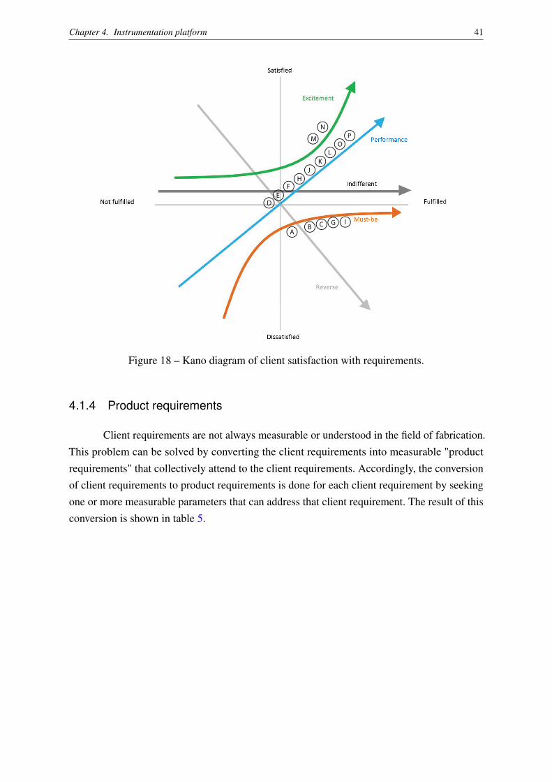
The Kano Model of Customer Satisfaction classifies product attributes based on howthey are perceived by customers and their effect on customer satisfaction. This classificationsis useful for guiding project decisions, because they indicate when good is good enough, andwhen more is better. The Kano diagram for this project is shown in figure 18.
Chapter 4. Instrumentation platform 41
P
N
OM
L
I
H
AB
C
D
E
F
G
J
K
Figure 18 – Kano diagram of client satisfaction with requirements.
4.1.4 Product requirements
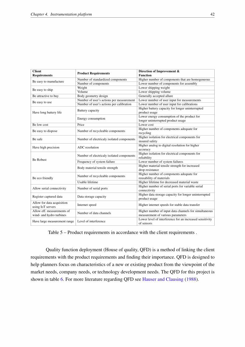
Client requirements are not always measurable or understood in the field of fabrication.This problem can be solved by converting the client requirements into measurable "productrequirements" that collectively attend to the client requirements. Accordingly, the conversionof client requirements to product requirements is done for each client requirement by seekingone or more measurable parameters that can address that client requirement. The result of thisconversion is shown in table 5.
Chapter 4. Instrumentation platform 42
ClientRequirements Product Requirements Direction of Improvement &
Function
Be easy to manufactureNumber of standardized components Higher number of components that are homogeneousNumber of components Lower number of components for assembly
Be easy to shipWeight Lower shipping weightVolume Lower shipping volume
Be attractive to buy Body geometry design Generally accepted allure
Be easy to useNumber of user’s actions per measurement Lower number of user input for measurementsNumber of user’s actions per calibration Lower number of user input for calibrations
Have long battery lifeBattery capacity
Higher battery capacity for longer uninterruptedproduct usage
Energy consumptionLower energy consumption of the product forlonger uninterrupted product usage
Be low cost Price Lower cost
Be easy to dispose Number of recycleable componentsHigher number of components adequate forrecycling
Be safe Number of electricaly isolated componentsHigher isolation for electrical components forinsured safety
Have high precision ADC resolutionHigher analog to digital resolution for higheraccuracy
Be RobustNumber of electricaly isolated components
Higher isolation for electrical components forreliability
Frequency of system failure Lower number of system failures
Body material tensile strengthHigher material tensile strength for increaseddrop resistance
Be eco friendlyNumber of recycleable components
Higher number of components adequate forreusability of materials
Usable lifetime Higher lifetime for decreased material waste
Allow serial connectivity Number of serial portsHigher number of serial ports for variable serialconnectivity
Register captured data Data storage capacityHigher data storage capacity for longer uninterruptedproduct usage
Allow for data acquisitionusing IoT servers Internet speed Higher internet speeds for stable data transfer
Allow eff. measurements ofwind- and hydro turbines Number of data channels
Higher number of input data channels for simultaneousmeasurement of various parameters
Have large measurement range Level of interferenceLower level of interference for an increased sensitivityof sensors
Table 5 – Product requirements in accordance with the client requirements .
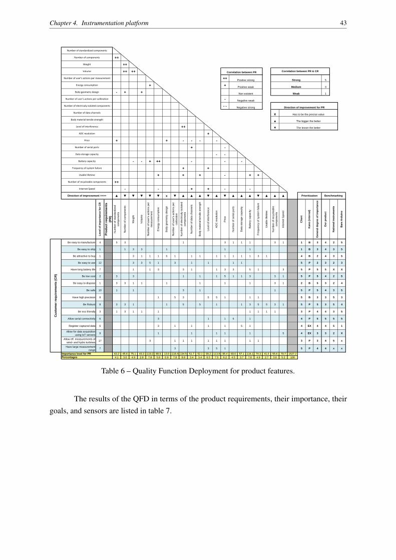
Quality function deployment (House of quality, QFD) is a method of linking the clientrequirements with the product requirements and finding their importance. QFD is designed tohelp planners focus on characteristics of a new or existing product from the viewpoint of themarket needs, company needs, or technology development needs. The QFD for this project isshown in table 6. For more literature regarding QFD see Hauser and Clausing (1988).
Chapter 4. Instrumentation platform 43
++
++
++ ++
++ 5
+ + 3
- + + 1
-
- -
x
++
+
+ + - - - -
+ -
- -
- - + ++ - - -
+ +
+ + + - + +
++
- - + + - -
x
Lev
el o
f im
po
rtan
ce f
or
CR
Pro
du
ct r
equ
irem
ents
(P
R)
Num
ber
of s
tand
ardi
zed
com
pone
nts
Num
ber
of c
ompo
nent
s
Wei
ght
Vol
ume
Num
ber
of u
ser's
act
ions
per
m
easu
rem
ent
Ene
rgy
cons
umpt
ion
Bod
y ge
omet
ry d
esig
n
Num
ber
of u
ser's
act
ions
per
ca
libra
tion
Num
ber
of e
lect
rical
y is
olat
ed
com
pone
nts
Num
ber
of d
ata
chan
nels
Bod
y m
ater
ial t
ensi
le s
tren
gth
Leve
l of i
nter
fere
nce
AD
C r
esol
utio
n
Pric
e
Num
ber
of s
eria
l por
ts
Dat
a st
orag
e ca
paci
ty
Bat
tery
cap
acity
Fre
quen
cy o
f sys
tem
failu
re
Usa
ble
lifet
ime
Num
ber
of r
ecyc
leab
le
com
pone
nts
Inte
rnet
Spe
ed
Clie
nt
Kan
o (
inte
rnal
)
Gen
eral
deg
ree
of
imp
ort
ance
Ou
r p
rod
uct
Nat
ion
al in
stru
men
ts
Bar
e A
rdu
ino
Be easy to manufacture 4 5 3 1 3 1 1 1 3 1 1 B 3 4 2 5
Be easy to ship 1 1 3 3 1 1 1 1 B 3 4 3 5
Be attractive to buy 1 3 1 1 1 5 1 1 1 1 1 1 1 1 3 1 4 B 2 4 3 5
Be easy to use 12 3 3 5 1 3 1 1 1 1 5 P 2 3 2 3
Have long battery life 7 1 1 3 3 1 1 3 3 5 1 3 5 P 5 5 X X
Be low cost 2 3 3 1 1 1 5 1 1 3 3 1 5 P 5 4 2 5
Be easy to dispose 1 3 3 1 1 1 1 1 1 3 1 2 B 5 3 2 4
Be safe 10 1 1 3 1 1 5 P 5 4 3 5
Have high precision 8 1 5 3 5 5 1 1 1 5 B 3 3 5 3
Be Robust 8 3 3 1 1 5 5 1 1 3 5 5 3 1 5 P 5 3 5 4
Be eco friendly 3 1 3 1 1 1 1 1 1 1 3 P 4 4 3 5
Allow serial connectivity 6 3 1 1 5 1 4 P 5 5 5 5
Register captured data 6 3 1 1 1 1 5 1 4 EX 4 4 5 1
Allow for data acquisition using IoT servers
9 1 1 1 1 1 5 4 EX 3 3 2 X
Allow eff. measurements of wind- and hydro turbines
17 3 1 1 1 1 1 1 1 1 3 P 3 4 5 x
Have large measurement range
7 3 3 5 1 5 P 4 4 x x
63.2 45.6 75.1 43.3 119.2 88.9 13.0 118.4 134.5 51.7 52.1 99.2 113.8 95.4 69.0 57.1 116.1 74.3 41.8 55.6 79.7 1527.24.1 3.0 4.9 2.8 7.8 5.8 0.9 7.8 8.8 3.4 3.4 6.5 7.5 6.2 4.5 3.7 7.6 4.9 2.7 3.6 5.2 100
Number of standardized components
Energy consumption
Number of user's actions per measurement
Volume
Weight
Number of components
Correlation between PR & CRCorrelation between PR
Positive strong Strong
Medium
Weak
Positive weak
Non existent
Negative weak
Cu
sto
mer
req
uir
emen
ts (
CR
)
Number of serial ports
The bigger the better
Data storage capacity
The lesser the better
Battery capacity
Frequency of system failure
Usable lifetime
Level of interference
ADC resolution
Price
Number of data channels
Body material tensile strength
Number of recycleable components
Importance level for PRPercentages
Body geometry design
Number of user's actions per calibration
Internet Speed
Direction of improvement >>>> Prioritization
Direction of improvement for PR
Has to be the precise value
Negative strong
Benchmarking
Number of electricaly isolated components
Table 6 – Quality Function Deployment for product features.
The results of the QFD in terms of the product requirements, their importance, theirgoals, and sensors are listed in table 7.

Chapter 4. Instrumentation platform 44
QFDScore Product requirements Objective Units Goal Sensor Unwanted Results
8.5Number of electricallyisolated components
High number ofcomponent isolation Number
All componentsshielded and isolated Counter
No shieldedcomponents
8.1 Battery capacityHigh battery capacityfor enhanced time of
usemAh Minimum 3500 mAh Wattmeter
Lessthan 3500 mAh
7.6 Price Low price $ Maximum $100 Price More than $100
7.4Number of user’s
actions per measurement
Minimal manualactions per
measurementNumber Least number of actions Counter More than 7
7.1 ADC resolutionHigh ADC resolutionfor enhanced precision bits Minimum 8 bits Tests Less than 8 bits
7.1Number of user’s
actions per calibrationMinimal manual
actions for calibration Number Least number of actions CounterDifficult
calibrationprocess
5.9Level of
interference
Low noise andinterference formeasurements
dB Maximum 5 dB Oscilloscope More than 15 dB
5.6 WeightLight weightfor shipping Kg Maximum 1 kg Balance More than 2 kg
5.5Energy
consumptionLow energyconsumption Watt Maximum 100 mAh Wattmeter More than 400 mAh
5.2 Internet SpeedHigher internet speedsfor stable data transfer kbps Minimum 512 kbps Speedtest Less than 64kbps
4.8Number of
standardized components
High number ofstandardized-readily-available components
NumberMaximum number of
standardized components CounterNo standardized
components
4.7 Number of serial portsNumber of Serialcommunication
capabilitiesNumber At least 1 port Counter No serial ports
4.5Frequency ofsystem failure
Low occurrences ofsystem failure Hz 0 Hz Tests More than 1 Hz
4.3Number of
recyclable componentsHigh number of
recyclable components Number All components recyclable CounterNo recyclablecomponents
3.9 Data storage capacityLarge space for data
saving bytes Minimum 2 Gb Datasheet No data storage
3.5Body materialtensile strength
High tensile strengthfor durability of body Pa 100 Mpa minimum Tests less than 20 Mpa
3.2Number of data
channels
High number of inputfor measurement ofvarious parameters
Number 40 minimum Counter Less than 30
2.6Number ofcomponents
Low number ofcomponents for
assemblingNumber Least number of components Counter
High number ofcomponents
2.6 VolumeSmall dimensions for
shipping m3 Maximum 0.0015 m3 RulerMore than0.0030 m3
2.5 Usable lifetime Long life of usage Years Minimum 5 year life ClockLess than one
year
0.8 Body geometry designAttractive and robust
design Attractive OpinionsUnattractive
design
Table 7 – Product requirements.
4.2 Conceptual design
The conceptual design phase of a project is one of the most decisive parts for thesuccess of a product, because this phase encapsulates the inception of solutions, which requirescreativity to meet or surpass the product requirements in a unique and most efficient manner,
Chapter 4. Instrumentation platform 45
compared to the concurrents. As such, the product requirements obtained in the informationalphase form the basis of the search for solutions and alternative solutions.
4.2.1 Functional structure of the product
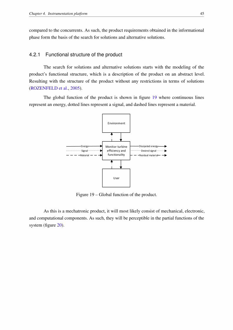
The search for solutions and alternative solutions starts with the modeling of theproduct’s functional structure, which is a description of the product on an abstract level.Resulting with the structure of the product without any restrictions in terms of solutions(ROZENFELD et al., 2005).
The global function of the product is shown in figure 19 where continuous linesrepresent an energy, dotted lines represent a signal, and dashed lines represent a material.
Monitor turbine efficiency and functionality
Energy
Signal
Material
Dissipated energy
Desired signal
Residual material
Environment
User
Figure 19 – Global function of the product.
As this is a mechatronic product, it will most likely consist of mechanical, electronic,and computational components. As such, they will be perceptible in the partial functions of thesystem (figure 20).
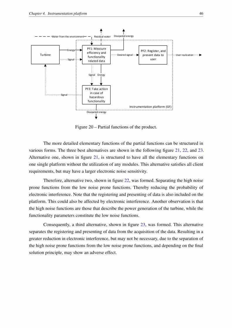
Chapter 4. Instrumentation platform 46
PF1: Measure efficiency and functionality related data
Energy
Dissipated energy
Desired signal
Residual water
Turbine
Water from the environment
Signal
PF3: Take action in case of hazardous
functionality
Signal Energy
Dissipated energy
PF2: Register, and present data to
user
Signal
Instrumentation platform (GF)
User realization
Figure 20 – Partial functions of the product.
The more detailed elementary functions of the partial functions can be structured invarious forms. The three best alternatives are shown in the following figure 21, 22, and 23.Alternative one, shown in figure 21, is structured to have all the elementary functions onone single platform without the utilization of any modules. This alternative satisfies all clientrequirements, but may have a larger electronic noise sensitivity.
Therefore, alternative two, shown in figure 22, was formed. Separating the high noiseprone functions from the low noise prone functions. Thereby reducing the probability ofelectronic interference. Note that the registering and presenting of data is also included on theplatform. This could also be affected by electronic interference. Another observation is thatthe high noise functions are those that describe the power generation of the turbine, while thefunctionality parameters constitute the low noise functions.
Consequently, a third alternative, shown in figure 23, was formed. This alternativeseparates the registering and presenting of data from the acquisition of the data. Resulting in agreater reduction in electronic interference, but may not be necessary, due to the separation ofthe high noise prone functions from the low noise prone functions, and depending on the finalsolution principle, may show an adverse effect.
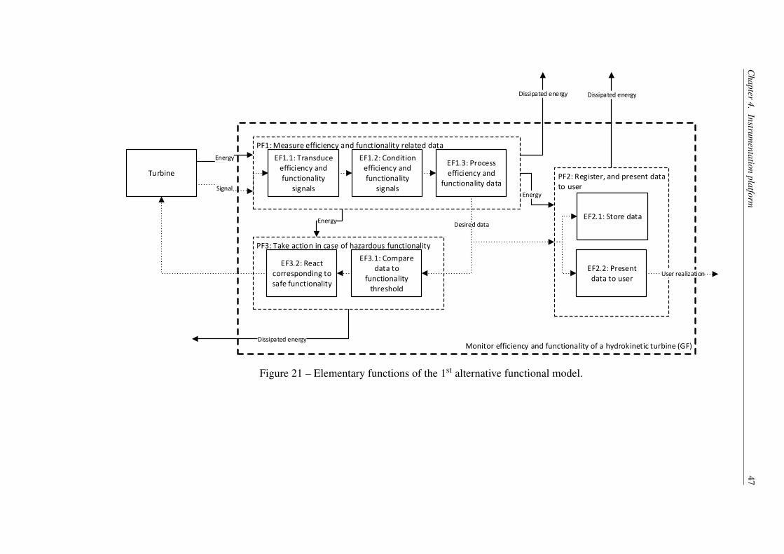
Chapter
4.Instrum
entationplatform
47
PF1: Measure efficiency and functionality related data
Energy
Dissipated energy
Desired data
Turbine
Signal
PF3: Take action in case of hazardous functionality
Energy
Dissipated energy
PF2: Register, and present data to user
Monitor efficiency and functionality of a hydrokinetic turbine (GF)
User realization
EF1.1: Transduce efficiency and functionality
signals
EF1.2: Condition efficiency and functionality
signals
EF1.3: Process efficiency and
functionality data
EF3.1: Compare data to
functionality threshold
EF3.2: React corresponding to safe functionality
EF2.1: Store data
EF2.2: Present data to user
Energy
Dissipated energy
Figure 21 – Elementary functions of the 1st alternative functional model.
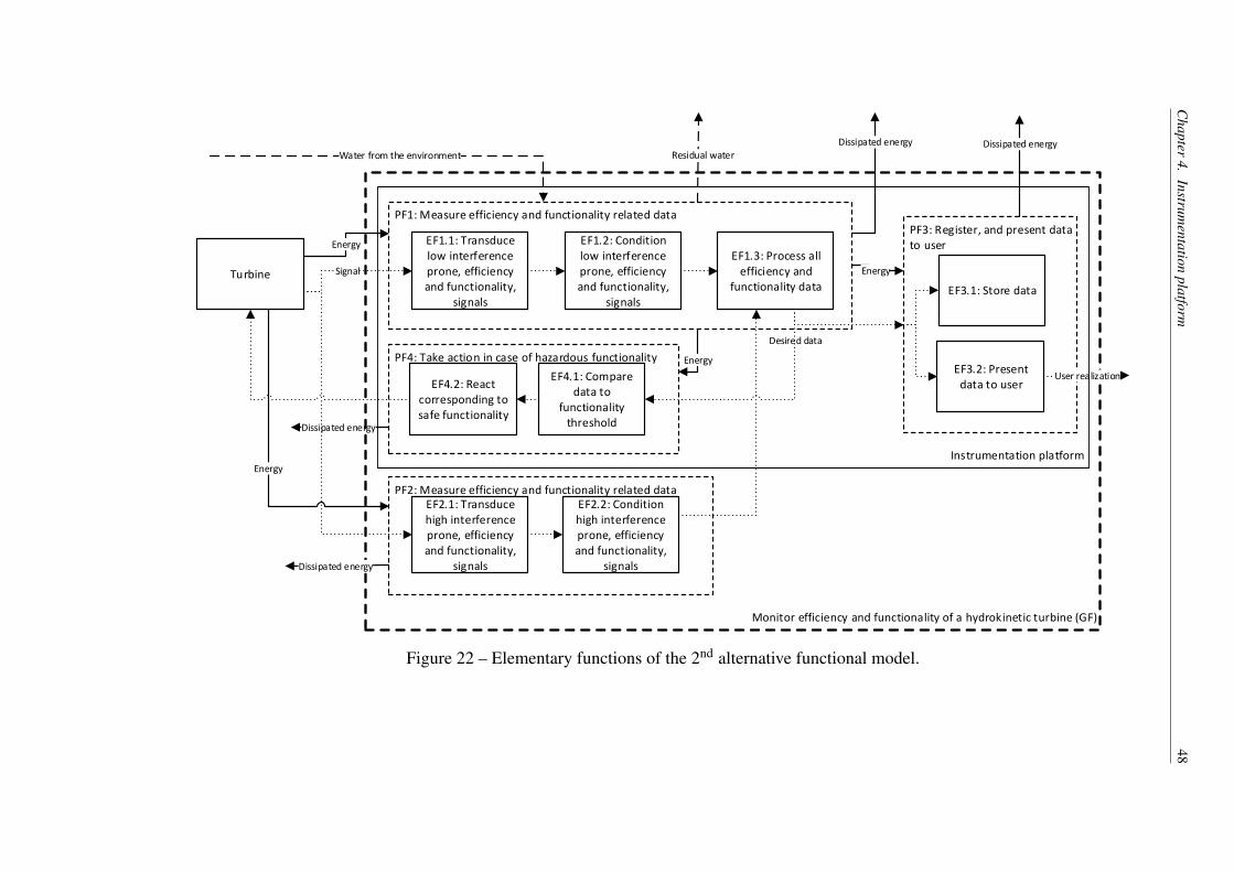
Chapter
4.Instrum
entationplatform
48
PF1: Measure efficiency and functionality related data
Energy
Dissipated energy
Desired data
Residual water
Turbine
Water from the environment
Signal
PF4: Take action in case of hazardous functionality Energy
Dissipated energy
PF3: Register, and present data to user
Monitor efficiency and functionality of a hydrokinetic turbine (GF)
User realization
EF1.1: Transduce low interference prone, efficiency and functionality,
signals
EF1.2: Condition low interference prone, efficiency and functionality,
signals
EF1.3: Process all efficiency and
functionality data
EF4.1: Compare data to
functionality threshold
EF4.2: React corresponding to safe functionality
EF3.1: Store data
EF3.2: Present data to user
Energy
Dissipated energy
EF2.1: Transduce high interference prone, efficiency and functionality,
signals
EF2.2: Condition high interference prone, efficiency and functionality,
signals
PF2: Measure efficiency and functionality related data
Energy
Dissipated energy
Instrumentation platform
Figure 22 – Elementary functions of the 2nd alternative functional model.
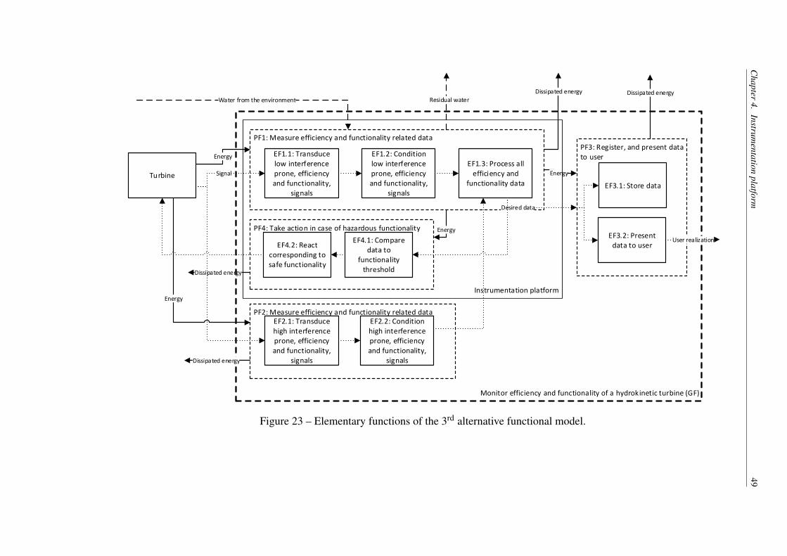
Chapter
4.Instrum
entationplatform
49
PF1: Measure efficiency and functionality related data
Energy
Dissipated energy
Desired data
Residual water
Turbine
Water from the environment
Signal
PF4: Take action in case of hazardous functionality Energy
Dissipated energy
PF3: Register, and present data to user
Monitor efficiency and functionality of a hydrokinetic turbine (GF)
User realization
EF1.1: Transduce low interference prone, efficiency and functionality,
signals
EF1.2: Condition low interference prone, efficiency and functionality,
signals
EF1.3: Process all efficiency and
functionality data
EF4.1: Compare data to
functionality threshold
EF4.2: React corresponding to safe functionality
EF3.1: Store data
EF3.2: Present data to user
Energy
Dissipated energy
EF2.1: Transduce high interference prone, efficiency and functionality,
signals
EF2.2: Condition high interference prone, efficiency and functionality,
signals
PF2: Measure efficiency and functionality related data
Energy
Dissipated energy
Instrumentation platform
Figure 23 – Elementary functions of the 3rd alternative functional model.

Chapter 4. Instrumentation platform 50
Client requirements ImportanceAlternatives
for the functional structure of the productAlternative 1 Alternative 2 Alternative 3
Allow eff.measurements of wind- and hydro turbines 5 3 5 5
Be easy to use 4 1 5 3Be safe 4 1 3 3Allow for data acquisition using IoTservers 3 3 5 3
Be low cost 3 3 3 3Be Robust 3 3 5 5Have high precision 3 3 3 3Have long battery life 2 3 3 3Allow serial connectivity 2 3 3 3Register captured data 2 5 5 5Have large measurement range 2 3 5 5Be easy to manufacture 2 5 3 3Be eco friendly 1 3 3 3Be easy to ship 1 3 3 3Be attractive to buy 1 3 3 1Be easy to dispose 1 3 3 1Sum of "alternativescore" × "importance" 109 155 137
Table 8 – Selection matrix for the functional structure
Table 8 shows the selection matrix of the functional structure, comparing the afore-mentioned alternatives to find the best of the three by assigning values of the degree in whichthe structure satisfies the client requirements, where 5 represents an excellent satisfaction, 3represents a good satisfaction, and 1 represents a weak satisfaction.
Alternative two presented the highest satisfaction of the three alternatives. And wastherefore selected as the product’s functional structure.
4.2.2 The search for alternative solutions and concepts
Each elementary function of the selected function structure (see figure 22) has variouspossibilities of solutions. Identifying them, requires one’s imagination, and increases thechance of the product’s success, by considering all possible solutions, and selecting the mostappropriate solution satisfying the client requirements.
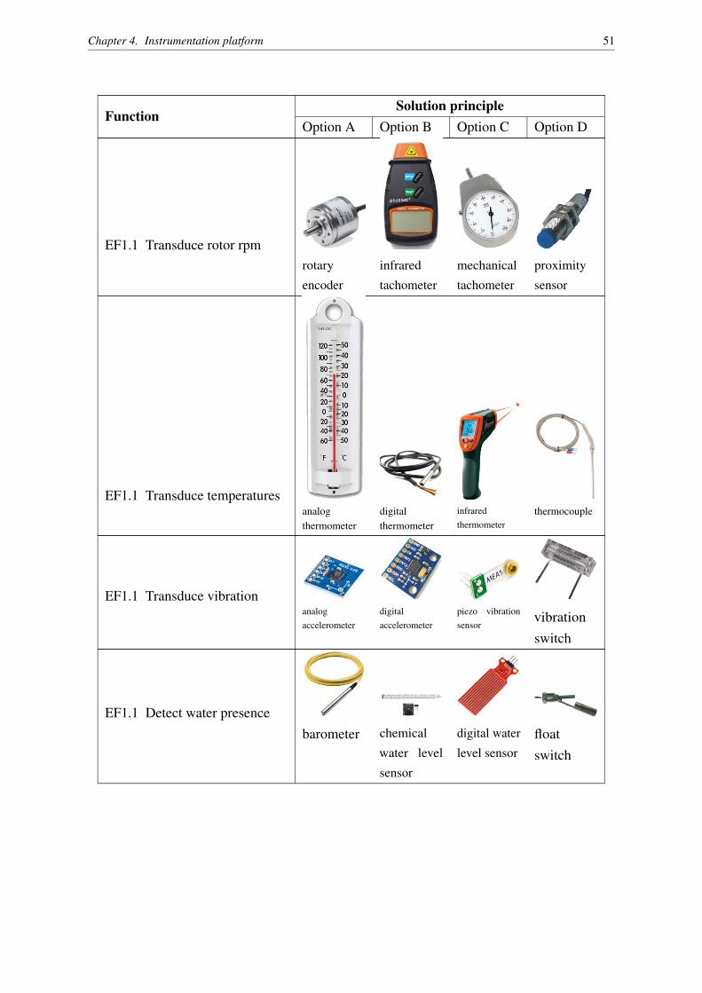
Chapter 4. Instrumentation platform 51
FunctionSolution principle
Option A Option B Option C Option D
EF1.1 Transduce rotor rpmrotary
encoder
infrared
tachometer
mechanical
tachometer
proximity
sensor
EF1.1 Transduce temperaturesanalogthermometer
digitalthermometer
infraredthermometer
thermocouple
EF1.1 Transduce vibrationanalogaccelerometer
digitalaccelerometer
piezo vibrationsensor
vibrationswitch
EF1.1 Detect water presencebarometer chemical
water level
sensor
digital water
level sensorfloatswitch
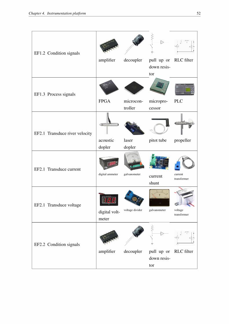
Chapter 4. Instrumentation platform 52
EF1.2 Condition signalsamplifier decoupler pull up or
down resis-tor
RLC filter
EF1.3 Process signalsFPGA microcon-
trollermicropro-cessor
PLC
EF2.1 Transduce river velocityacousticdopler
laserdopler
pitot tube propeller
EF2.1 Transduce currentdigital ammeter galvanometer current
shunt
currenttransformer
EF2.1 Transduce voltagedigital volt-meter
voltage divider galvanometer voltagetransformer
EF2.2 Condition signalsamplifier decoupler pull up or
down resis-tor
RLC filter
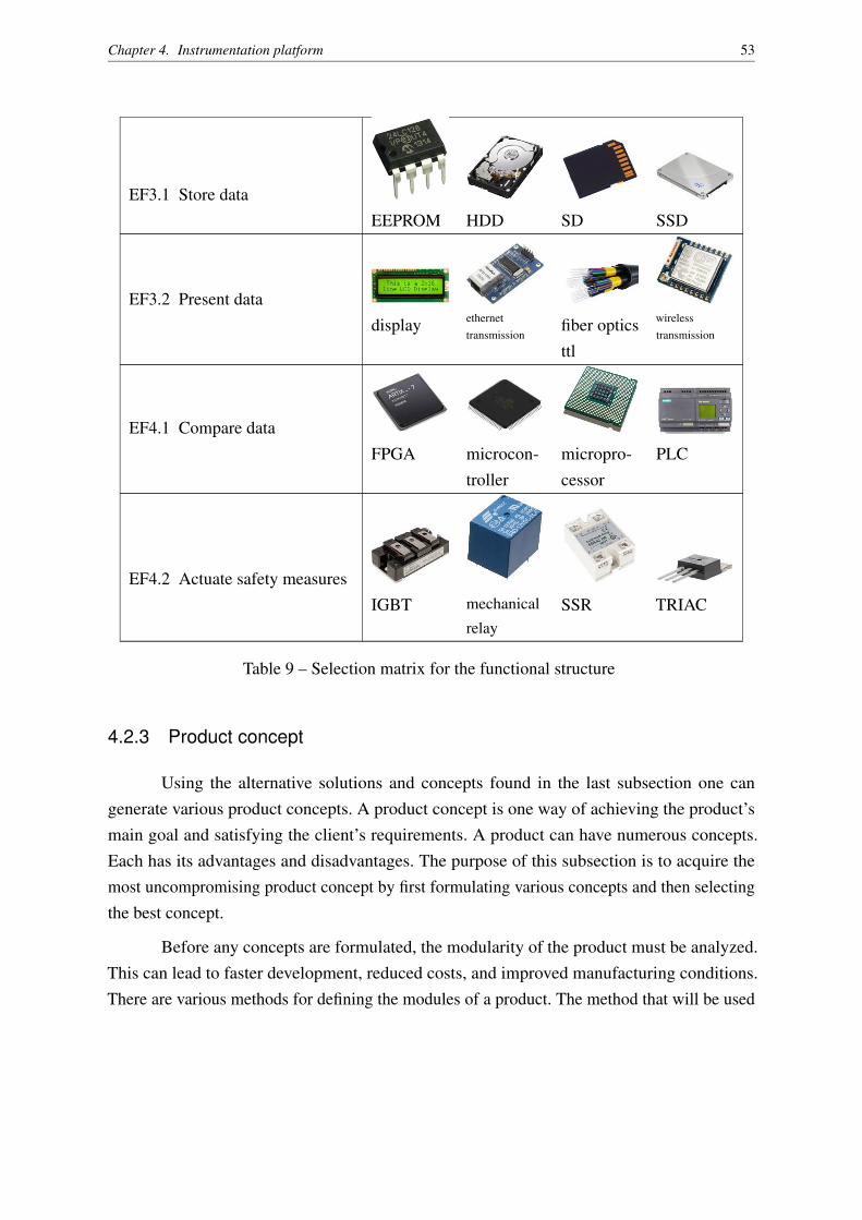
Chapter 4. Instrumentation platform 53
EF3.1 Store dataEEPROM HDD SD SSD
EF3.2 Present datadisplay ethernet
transmissionfiber opticsttl
wirelesstransmission
EF4.1 Compare dataFPGA microcon-
trollermicropro-cessor
PLC
EF4.2 Actuate safety measuresIGBT mechanical
relaySSR TRIAC
Table 9 – Selection matrix for the functional structure
4.2.3 Product concept
Using the alternative solutions and concepts found in the last subsection one cangenerate various product concepts. A product concept is one way of achieving the product’smain goal and satisfying the client’s requirements. A product can have numerous concepts.Each has its advantages and disadvantages. The purpose of this subsection is to acquire themost uncompromising product concept by first formulating various concepts and then selectingthe best concept.
Before any concepts are formulated, the modularity of the product must be analyzed.This can lead to faster development, reduced costs, and improved manufacturing conditions.There are various methods for defining the modules of a product. The method that will be used
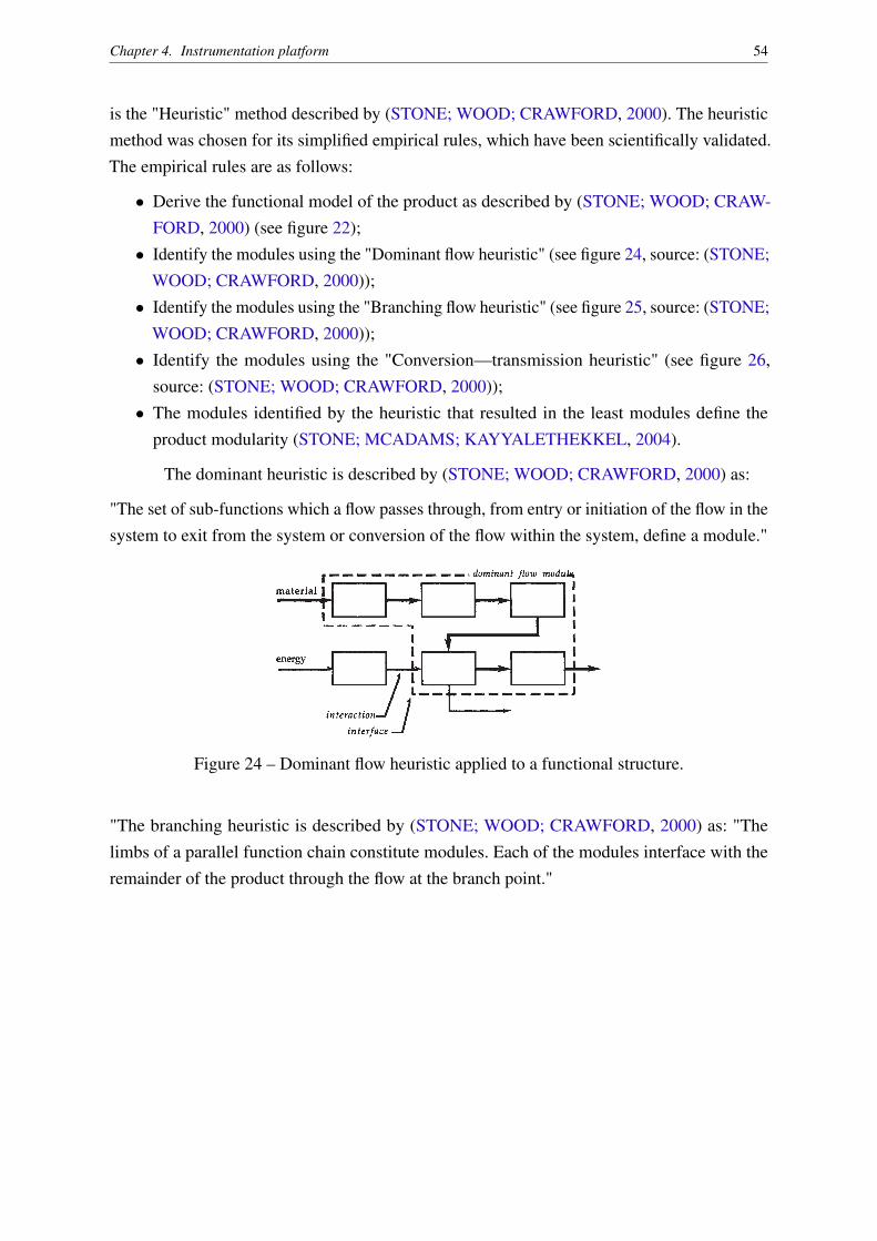
Chapter 4. Instrumentation platform 54
is the "Heuristic" method described by (STONE; WOOD; CRAWFORD, 2000). The heuristicmethod was chosen for its simplified empirical rules, which have been scientifically validated.The empirical rules are as follows:
• Derive the functional model of the product as described by (STONE; WOOD; CRAW-FORD, 2000) (see figure 22);• Identify the modules using the "Dominant flow heuristic" (see figure 24, source: (STONE;
WOOD; CRAWFORD, 2000));• Identify the modules using the "Branching flow heuristic" (see figure 25, source: (STONE;
WOOD; CRAWFORD, 2000));• Identify the modules using the "Conversion—transmission heuristic" (see figure 26,
source: (STONE; WOOD; CRAWFORD, 2000));• The modules identified by the heuristic that resulted in the least modules define the
product modularity (STONE; MCADAMS; KAYYALETHEKKEL, 2004).
The dominant heuristic is described by (STONE; WOOD; CRAWFORD, 2000) as:
"The set of sub-functions which a flow passes through, from entry or initiation of the flow in thesystem to exit from the system or conversion of the flow within the system, define a module."
heuristic, discuss which ones exist and which ones present opportunitiesfor a more modular design.
3.1 Dominant flowThe dominant flow heuristic examines each non-branching flow of a func-tion structure and groups the sub-functions the flow travels through untilit exits the system or is transformed into another flow. The identified setof sub-functions defines a module that deals with the flow traced throughthe system. The identified sub-functions form the boundary, orinterface,of the module. Any other flows, in addition to the traced flow, that crossthe boundary areinteractionsbetween the module and the remaining pro-duct. A dominant flow module is shown schematically in Figure 7. Toimplement the module, conduits must be specified to carry the interactionsacross the interface.
Stated succinctly, the dominant flow heuristic is:
Heuristic 1: The set of sub-functions which a flow passes through, fromentry or initiation of the flow in the system to exit from the system orconversion of the flow within the system, define a module.
3.1.1 Screwdriver—identified modulesIn the SKIL Twist power screwdriver, the flowelectricity passes throughfive sub-functions as outlined by a dashed rectangle shown in Figure 8.The sub-functionsstore electricity, supply electricity, transmit electricity,actuate electricityand regulate electricityall operate on the flow elec-tricity. The dominant flow heuristic identifies that these sub-functions couldbe combined as one module, which we name thesupply electricity module.
The next flow to trace is thebit. It first enters the system and traces throughthe two sub-functionscouple solidandsecure solid. This set of sub-func-tions forms a module that we call thecoupling module. The flowhandidentifies a superset of thecoupling modulewhich also encompasses the
A heuristic method for identifying modules for product architectures 15
Figure 7 Dominant flow
heuristic applied to a gen-
eric function structure
Figure 24 – Dominant flow heuristic applied to a functional structure.
"The branching heuristic is described by (STONE; WOOD; CRAWFORD, 2000) as: "Thelimbs of a parallel function chain constitute modules. Each of the modules interface with theremainder of the product through the flow at the branch point."
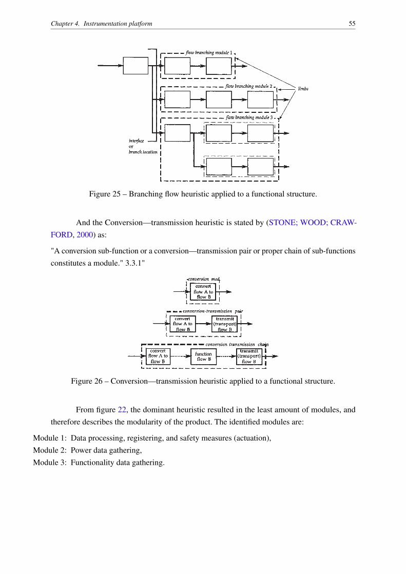
Chapter 4. Instrumentation platform 55
defined geometric connections, like various end mill attachments on a mill-ing machine. Other times, the interface may be fuzzier, like the differinginteractions between human force and the SKIL Twist power screwdriver.
The branching flow heuristic is stated formally as:
Heuristic 2: The limbs of a parallel function chain constitute modules. Eachof the modules interface with the remainder of the product through theflow at the branch point.
3.2.1 Screwdriver—identified modulesThe power screwdriver has three flows that branch, thebit, screw andhuman force. The flowhuman forceis examined first. Following the sub-function import human force, the flow branches into four limbs. Each limbrepresents a module as shown in Figure 12. The four identified modules arethe coupling/decoupling, manual use, actuatingand weight transmissionmodules. Note that a subset of thecoupling/decouplingmodule was ident-ified by the dominant flow heuristic. Theactuatemodule is a subset of thesupply electricitymodule identified by the dominant flow heuristic. Themanual useandweight transmissionmodules are new.
The branching flow of bit identifies two possible modules:decouplingandbit-transmission. Thedecouplingmodule, together with thecouplingmod-ule of the dominant flow heuristic, constitutes thecoupling/decouplingmodule already identified. Thebit-transmissionmodule is a subset of apreviously identified module.
A heuristic method for identifying modules for product architectures 19
Figure 11 Flow branching
heuristic applied to a gen-
eric function structure
Figure 25 – Branching flow heuristic applied to a functional structure.
And the Conversion—transmission heuristic is stated by (STONE; WOOD; CRAW-FORD, 2000) as:
"A conversion sub-function or a conversion—transmission pair or proper chain of sub-functionsconstitutes a module." 3.3.1"
the weight transmissionmodule is essentially the plastic casing of thescrewdriver.
A few remarks about the heuristics usage thus far are warranted. It isevident that they identify overlapping modules in some cases. At this point,we wonder which module to embody in such a case. Section 6 of thispaper discusses extensions to this work, including a customer needsapproach, which provide a means of determining which module toimplement. For now, we make the observation that the more ways a moduleis identified (in terms of heuristics and flows), the more important it is toimplement (since it must be associated with more customer needs).
3.3 Conversion—transmission modulesThe third heuristic method deals with conversion sub-functions and conver-sion to transmission chains. Conversion sub-functions accept a flow ofmaterial or energy and convert the flow to another form of material orenergy. In standard verb—object form, a conversion sub-function appearsasconvertflow A to flow B. In many cases, these conversion sub-functionsare already components or modules themselves. For instance, electricalmotors, hydraulic cylinders, and electrical heaters can all be representedby a single conversion sub-function and exist physically as a single compo-nent. If, additionally, a conversion sub-function exists in a chain with atransmit sub-function (or transport sub-function for material flow), then thechain presents an opportunity to form a module. This converts an energyor material to another form and then implements (transmits or transports)that new form of energy or material.
The method of the conversion—transmission heuristic, shown sche-matically in Figure 13, is simple. The essential actions are as follows:identify conversion sub-functions and check for transmit or transportsub-functions downstream of the converted flow. If none exist, then theconversion sub-function is a module by itself. If transmit or transport
A heuristic method for identifying modules for product architectures 21
Figure 13 Conversion—
transmission applied to a
generic set of sub-functions
Figure 26 – Conversion—transmission heuristic applied to a functional structure.
From figure 22, the dominant heuristic resulted in the least amount of modules, andtherefore describes the modularity of the product. The identified modules are:
Module 1: Data processing, registering, and safety measures (actuation),Module 2: Power data gathering,Module 3: Functionality data gathering.
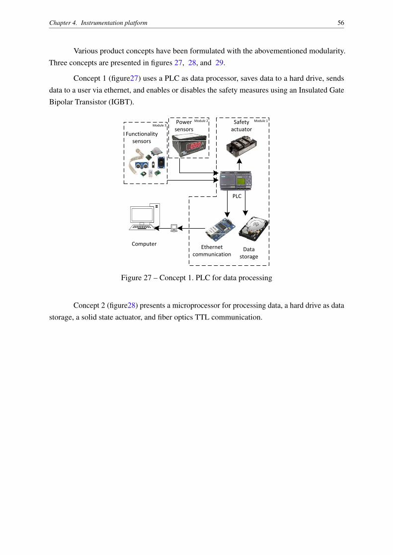
Chapter 4. Instrumentation platform 56
Various product concepts have been formulated with the abovementioned modularity.Three concepts are presented in figures 27, 28, and 29.
Concept 1 (figure27) uses a PLC as data processor, saves data to a hard drive, sendsdata to a user via ethernet, and enables or disables the safety measures using an Insulated GateBipolar Transistor (IGBT).
Safety
actuator
Power
sensorsFunctionality
sensors
PLC
Data
storage
Ethernet
communication
Computer
Module 1Module 2
Module 3
Safety
actuatorPower
sensors
Functionality
sensors
Microprocessor
Data
storage
Fiber optic
communication
Computer
Module 1Module 2
Module 3
Safety
actuator
Power
sensors
Functionality
sensors
Microcontroller
Data
storage
WiFi
communication
Computer
Module 1Module 2
Module 3
Figure 27 – Concept 1. PLC for data processing
Concept 2 (figure28) presents a microprocessor for processing data, a hard drive as datastorage, a solid state actuator, and fiber optics TTL communication.
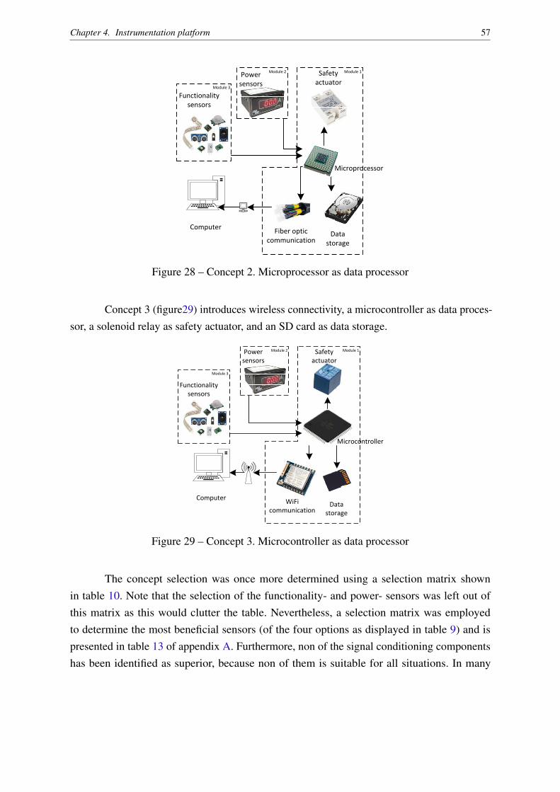
Chapter 4. Instrumentation platform 57
Safety
actuator
Power
sensorsFunctionality
sensors
PLC
Data
storage
Ethernet
communication
Computer
Module 1Module 2
Module 3
Safety
actuatorPower
sensors
Functionality
sensors
Microprocessor
Data
storage
Fiber optic
communication
Computer
Module 1Module 2
Module 3
Safety
actuator
Power
sensors
Functionality
sensors
Microcontroller
Data
storage
WiFi
communication
Computer
Module 1Module 2
Module 3
Figure 28 – Concept 2. Microprocessor as data processor
Concept 3 (figure29) introduces wireless connectivity, a microcontroller as data proces-sor, a solenoid relay as safety actuator, and an SD card as data storage.
Safety
actuator
Power
sensorsFunctionality
sensors
PLC
Data
storage
Ethernet
communication
Computer
Module 1Module 2
Module 3
Safety
actuatorPower
sensors
Functionality
sensors
Microprocessor
Data
storage
Fiber optic
communication
Computer
Module 1Module 2
Module 3
Safety
actuator
Power
sensors
Functionality
sensors
Microcontroller
Data
storage
WiFi
communication
Computer
Module 1Module 2
Module 3
Figure 29 – Concept 3. Microcontroller as data processor
The concept selection was once more determined using a selection matrix shownin table 10. Note that the selection of the functionality- and power- sensors was left out ofthis matrix as this would clutter the table. Nevertheless, a selection matrix was employedto determine the most beneficial sensors (of the four options as displayed in table 9) and ispresented in table 13 of appendix A. Furthermore, non of the signal conditioning componentshas been identified as superior, because non of them is suitable for all situations. In many
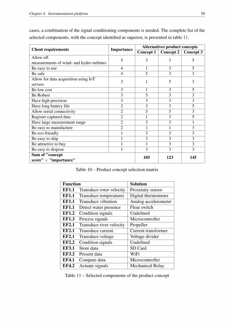
Chapter 4. Instrumentation platform 58
cases, a combination of the signal conditioning components is needed. The complete list of theselected components, with the concept identified as superior, is presented in table 11.
Client requirements Importance Alternatives product conceptsConcept 1 Concept 2 Concept 3
Allow eff.measurements of wind- and hydro turbines 5 3 3 5
Be easy to use 4 1 3 5Be safe 4 5 3 3Allow for data acquisition using IoTservers 3 1 5 3
Be low cost 3 1 3 5Be Robust 3 5 3 3Have high precision 3 3 3 3Have long battery life 2 3 3 5Allow serial connectivity 2 5 5 3Register captured data 2 1 3 5Have large measurement range 2 3 3 1Be easy to manufacture 2 1 1 3Be eco friendly 1 3 3 3Be easy to ship 1 3 3 3Be attractive to buy 1 1 3 3Be easy to dispose 1 3 3 3Sum of "conceptscore" × "importance" 105 123 145
Table 10 – Product concept selection matrix
Function SolutionEF1.1 Transduce rotor velocity Proximity sensorEF1.1 Transduce temperatures Digital thermometerEF1.1 Transduce vibration Analog accelerometerEF1.1 Detect water presence Float switchEF1.2 Condition signals UndefinedEF1.3 Process signals MicrocontrollerEF2.1 Transduce river velocity PropellerEF2.1 Transduce current Current transformerEF2.1 Transduce voltage Voltage dividerEF2.2 Condition signals UndefinedEF3.1 Store data SD CardEF3.2 Present data WiFiEF4.1 Compare data MicrocontrollerEF4.2 Actuate signals Mechanical Relay
Table 11 – Selected components of the product concept
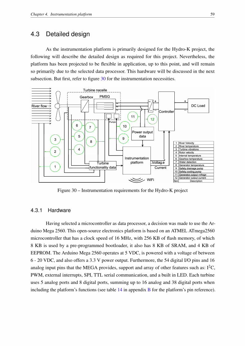
Chapter 4. Instrumentation platform 59
4.3 Detailed design
As the instrumentation platform is primarily designed for the Hydro-K project, thefollowing will describe the detailed design as required for this project. Nevertheless, theplatform has been projected to be flexible in application, up to this point, and will remainso primarily due to the selected data processor. This hardware will be discussed in the nextsubsection. But first, refer to figure 30 for the instrumentation necessities.
River flow
Turbine nacelle ----------------------- I
I
I
I
Gearbox PMSG ,---------,
Pumps
Turbine ------functionality data
+
DC Load =-i - !Controller
B Power output
data
Instrumentation platform lvo-lt_a _g_e,
Current
WiFi
1 I River Velocity 2 I River temperature 3 I Turbine vibrations 4 I Rotor velocity_ 5 !Internal temperature 6 I Gearbox tem_Qerature 7 I Water detection 8 I Generator temperature 9 I Safety drainage pump
10 I Safety cooling pump 11 I Generator output voltaae 12 I Generator out_Qut current Item I Description
Figure 30 – Instrumentation requirements for the Hydro-K project
4.3.1 Hardware
Having selected a microcontroller as data processor, a decision was made to use the Ar-duino Mega 2560. This open-source electronics platform is based on an ATMEL ATmega2560microcontroller that has a clock speed of 16 MHz, with 256 KB of flash memory, of which8 KB is used by a pre-programmed bootloader, it also has 8 KB of SRAM, and 4 KB ofEEPROM. The Arduino Mega 2560 operates at 5 VDC, is powered with a voltage of between6 - 20 VDC, and also offers a 3.3 V power output. Furthermore, the 54 digital I/O pins and 16analog input pins that the MEGA provides, support and array of other features such as: I2C,PWM, external interrupts, SPI, TTL serial communication, and a built in LED. Each turbineuses 5 analog ports and 8 digital ports, summing up to 16 analog and 38 digital ports whenincluding the platform’s functions (see table 14 in appendix B for the platform’s pin reference).

Chapter 4. Instrumentation platform 60
The maximum supported current on each of these pins is 20 mA, and 50 mA on the 3.3 V pin.A 10-bit ADC converts an input on its analog pins from 0 - 5 V into a digital signal from 0- 1024. The features that this electronics platform offers will safeguard the instrumentationplatform’s application flexibility.
The remaining hardware components of module 1 (defined in sub section 4.2.3) willbe described next. First, the WiFi component added to this module is an "ESP8266-07". Thiscomponent is low cost and offers: SPI, I2C, and TTL serial communication, a 10-bit ADC, aceramic antenna plus a U-FL connector, and has its own microcontroller running at 80 MHz.The TTL serial communication was used to communicate with the Arduino Mega. Note thata CC3000 WiFi shield has been tested and is discussed in sub section 4.4, but the final WiFicomponent is the ESP8266-07. Next, the safety actuation component is a JQX-3F mechanicalrelay which has a 5 V activation coil, a rated load of 10 A 250 VAC/30 VDC, and an insulationresistance capable of handling voltages greater than 1000 VAC/500 VDC. The last componentof module 1 is the SD Card. A standard SD Card slot was added to save data on an SD Card.The SD Card slot operates at 3.3 V or 5 V and uses the SPI protocol to communicate withthe Arduino Mega. Moreover, a "Tiny RTC" was included in module 1 to store the date andtime along with the data to the SD card. This RTC communicates with the Mega using the I2Cprotocol.
Module 2 (power data gathering) consists of a current transformer and a voltage divider.The selected current transformer is a SCT-013-000. This transformer was chosen for its lowprice and allows non-invasive AC-current measurements of up to 100 A and consists of a 2000turn coil. Interfacing this sensor with module 1 required signal conditioning. The calculationsfor this signal conditioning are described next.
First of all, measuring currents with the selected microcontroller is impossible. Thecurrent must somehow be transformed into a voltage between 0 - 5 V. The transformation canbe achieved with a burden resistor, which needs to be calculated to provide a good resolution.Due to the 2000 turns of its coil, the current transformer will decrease the measured current2000 times. And according to the generator specialist of the Hydro-K project, the maximumcurrent delivered by the generator is 35 A RMS. This means that the primary peak current willbe:
Primary peak current = RMS current×√
2 = 35A×√
2 = 49.50A
The secondary peak current will therefore be:
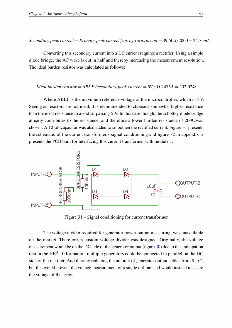
Chapter 4. Instrumentation platform 61
Secondary peak current =Primary peak current/no. o f turns in coil = 49.50A/2000= 24.75mA
Converting this secondary current into a DC current requires a rectifier. Using a simplediode bridge, the AC wave is cut in half and thereby increasing the measurement resolution.The ideal burden resistor was calculated as follows:
Ideal burden resistor = AREF/secondary peak current = 5V/0.02475A = 202.02Ω
Where AREF is the maximum reference voltage of the microcontroller, which is 5 V.Seeing as resistors are not ideal, it is recommended to choose a somewhat higher resistancethan the ideal resistance to avoid surpassing 5 V. In this case though, the schottky diode bridgealready contributes to the resistance, and therefore a lower burden resistance of 200Ωwaschosen. A 10 µF capacitor was also added to smoothen the rectified current. Figure 31 presentsthe schematic of the current transformer’s signal conditioning and figure 72 in appendix Epresents the PCB built for interfacing this current transformer with module 1.
100ohm
10uF
100ohm
D1 D2
D3 D4
BURDENRESISTOR
C1
INPUT-1
INPUT-2
OUTPUT-1
OUTPUT-2
BURDENRESISTOR1
Figure 31 – Signal conditioning for current transformer
The voltage divider required for generator power output measuring, was unavailableon the market. Therefore, a custom voltage divider was designed. Originally, the voltagemeasurement would be on the DC side of the generator output (figure 30) due to the anticipationthat in the HK3-10 formation, multiple generators could be connected in parallel on the DCside of the rectifier. And thereby reducing the amount of generator output cables from 9 to 2,but this would prevent the voltage measurement of a single turbine, and would instead measurethe voltage of the array.
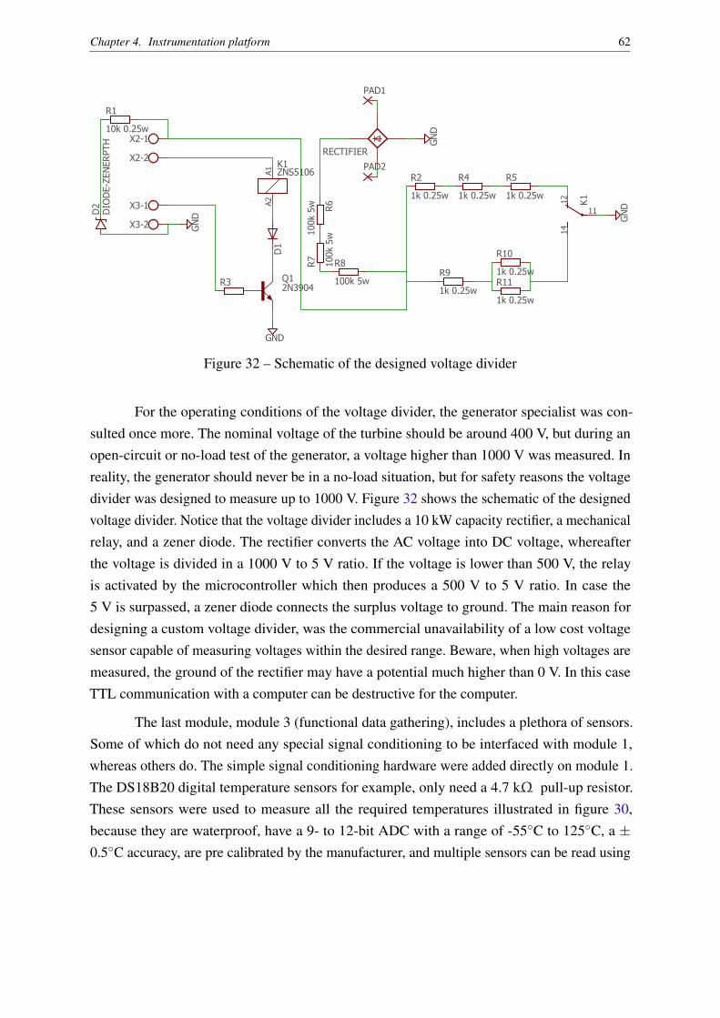
Chapter 4. Instrumentation platform 62
Spic
eO
rder
1Spic
eO
rder
2
ZNS5106
GND
2N3904
GN
D
GN
D
100k 5
w
100k 5
w
100k 5w
DIO
DE-Z
EN
ER
PTH
GN
D
1k 0.25w 1k 0.25w 1k 0.25w
1k 0.25w
1k 0.25w
1k 0.25w
10k 0.25w
K1
A2
A1
K1
12
14
11
D1
Q1
X2-1
X2-2
X3-1
X3-2
R3
R6
R7
R8
D2
RECTIFIER
R2 R4 R5
R9
R10
R11
R1
PAD1
PAD2
Figure 32 – Schematic of the designed voltage divider
For the operating conditions of the voltage divider, the generator specialist was con-sulted once more. The nominal voltage of the turbine should be around 400 V, but during anopen-circuit or no-load test of the generator, a voltage higher than 1000 V was measured. Inreality, the generator should never be in a no-load situation, but for safety reasons the voltagedivider was designed to measure up to 1000 V. Figure 32 shows the schematic of the designedvoltage divider. Notice that the voltage divider includes a 10 kW capacity rectifier, a mechanicalrelay, and a zener diode. The rectifier converts the AC voltage into DC voltage, whereafterthe voltage is divided in a 1000 V to 5 V ratio. If the voltage is lower than 500 V, the relayis activated by the microcontroller which then produces a 500 V to 5 V ratio. In case the5 V is surpassed, a zener diode connects the surplus voltage to ground. The main reason fordesigning a custom voltage divider, was the commercial unavailability of a low cost voltagesensor capable of measuring voltages within the desired range. Beware, when high voltages aremeasured, the ground of the rectifier may have a potential much higher than 0 V. In this caseTTL communication with a computer can be destructive for the computer.
The last module, module 3 (functional data gathering), includes a plethora of sensors.Some of which do not need any special signal conditioning to be interfaced with module 1,whereas others do. The simple signal conditioning hardware were added directly on module 1.The DS18B20 digital temperature sensors for example, only need a 4.7 kΩ pull-up resistor.These sensors were used to measure all the required temperatures illustrated in figure 30,because they are waterproof, have a 9- to 12-bit ADC with a range of -55C to 125C, a ±0.5C accuracy, are pre calibrated by the manufacturer, and multiple sensors can be read using
Chapter 4. Instrumentation platform 63
only one data bus. As temperature sensors are common for instrumentation purposes, theirpull-up resistors were added directly onto module 1.
Another sensor that was easily interfaced with module 1 is the LJ12A3 proximity sensorthat was used to measure the rotor’s rotational velocity. The sensor requires a power sourceof at least 12 V, and the output is binary (on = 12 V, off > 1.5 V). A simple 2-resistor voltagedivider changed the output voltage to a 5 V maximum. These resistors were also directly addedto module 1. The working principle of this sensor is that it detects metal cogs of a cogwheeladded to the rotor axle. Knowing the number of cogs, and the time elapsed between two cogs,one can calculate the rotational velocity.
The two most easily interfaced sensors were the water detection sensor, which was asimple On/Off floating switch, and the analog ADXL335 accelerometer. The accelerometermeasures vibrations in 2 axes, is supplied with 3.3 V, and also has an output of 3.3 V. Theoutput being 3.3 V, implies that no signal conditioning was needed.
The most challenging sensor interface was that of the FLOWATCH water velocitymeasuring impeller. Its operating principle is based on a magnet and a coil. The magnet rotateswith the impeller and every full rotation it induces a small alternating current in the waterproofcoil. The impeller comes in a kit complete with a handheld meter that can display the watervelocity in various units of speed. Interfacing this impeller with the Arduino Mega meantdesigning an amplifier, that could convert and amplify the small AC current into an AC voltagewith 5 V peak. Figure 33 shows the schematic of the designed amplifier. The impeller’s signalwas first filtered with an RC filter, afterwards the signal was amplified with an instrumentationalamplifier, which was made using three of the four op-amps of a LM324. The fourth op-ampwas used as a comparator, which switched to 5 V if a certain input voltage was passed andswitched back to 0 V if the input was under the voltage threshold. A correlation between theriver velocity and the time elapsed between two peaks could then be made. The calibration ofall the above sensors will be discussed in subsection 4.4 after the software design.

Chapter 4. Instrumentation platform 64
1k
100
100
100
1k100
100
GND
GND
GND
1k
1k
0.22uF
0.22uF
GND
GND
100
100
100
100 10k
1k
1k
2.2k
GND
10k
22k
LM324N
LM324N
LM324NLM324N
1M
100k
GND
10nF
0.1uF
GND
10uF
10k
R1
GAIN
R3
R4 R5R6
R7
V-1
V-2
VOUT-1
VOUT-2
VIN-1
VIN-2
R2
R8
C1
C2
R9
R10
R11
R12
R13
R14
R15
R16
R17
R18
2
3
1
IC2A
6
5
7
IC2B
IC2C
9
10
8
IC2D
13
12
14
411
R19R20
C3
C4 C5
R21
+
Figure 33 – Schematic for designed water flow sensor
The power for all these sensors and components is supplied by two 7000 mAH batteries(see figure 35a), which are projected to be charged by the turbine to ensure an uninterruptedpower supply.
4.3.2 Software development
To send instructions to the selected microcontroller, the Arduino Integrated Develop-ment Environment (IDE) was used along with the "Arduino programming language" Thislanguage is similar to C++ and a program in this language is called a sketch. In other words,using the Arduino programming language, one creates a sketch inside the IDE and uploads theinstructions to the microcontroller on the Arduino board. A sketch was made for each interfacedcomponent in order to test them. In order to create the final sketch which will integrated allcomponents, a Finite State Machine was first devised.
A Finite State Machine (FSM) is a mathematical model used for programming. Themachine can only be in one state at a time and can change from one state to another when acertain condition is met or an event occurs. Transition conditions are unique per state, whichmeans that there can never be two or more identical transition conditions leaving one state.The program can also remain a state with a transition condition that returns to the same state.All states and conditions should be analyzed in order to prevent any undefined conditions, i.e.,all possible situations must be anticipated. For these reasons, this type of model aids with theanticipation of lockups, and undesired functions. This is imperative for any programs intendedfor remote monitoring use. A simplified finite state machine diagram is shown in figure 34. The

Chapter 4. Instrumentation platform 65
legend for the diagram is shown in table 12. The simplifications that were made in this diagramare: the merging of the three types of anticipated dangers, and the simplification of the dataacquisition. If these simplifications were not made, the FSM would most likely consist of morethan 64 states. This would diminish clarity and contradict the purpose of the diagram.
The logic of the resulting FSM diagram is as follows. The setup state is the initialand final state, meaning the program never stops running. After the setup has completed,transition condition "A" is met, and the program transitions to state "1". In state "1" the programconstantly checks for safety parameters, acquires sensor data, checks for lockups using awatchdog timer, checks the time that has passed since the last data registration, and checksthe date. The safety parameters that are checked for are the temperatures inside the turbine,the presence of water inside the turbine (as a result of unwanted water infiltration into theturbine), and a high voltage output of the generator. A cooling pump is used to respond to hightemperatures, a drainage pump is activated in case of water presence, and a relay is switchedoff, increasing the resistance in case of high voltage. Responding to detected dangers is done instate "2" and "4". The responding action is also the only difference between state "1" and "2".Reading sensor data includes voltages, currents, temperatures, vibrations, rotational velocities,river velocity and temperature, and water presence. And if the elapsed time, between the lastdata registration and the current time, is larger than the time threshold of data registration, themachine enters state "3" or state "4" depending on whether there is a danger or not. In state "3"and "4" the acquired data is stored on an SD card with the time and sent to a server via ModbusIP/TCP. Note that in sub section 4.4 the "HTTP protocol" was first tested, but the Modbus IPprotocol proved to be more superior. Another detail is that the date is checked in order to savethe data from each day in a separate file. Hereby facilitating the data analysis at a later stage.
Implementing the FSM, resulted in a robust program. During the conception of the finalsketch, the logic of the FSM was maintained for the instrumentation of 1, 2, or 3 HK-10 turbines.Changing from one configuration to another only requires the program’s intial parameters tobe changed, as all of the program’s tasks were grouped into "functions". This made the sketchless cluttered and easier to reprogram. The final sketch is presented in appendix H, and bychanging parameters and uploading the adapted sketch to the microcontroller, it can servefor the instrumentation of 1, 2 or 3 HK-10 turbines. This completes the backend applicationfor informing an observer of the turbine functionality and the generator output. The backendapplication sends the data to a database, which is also part of the backend, via WiFi.
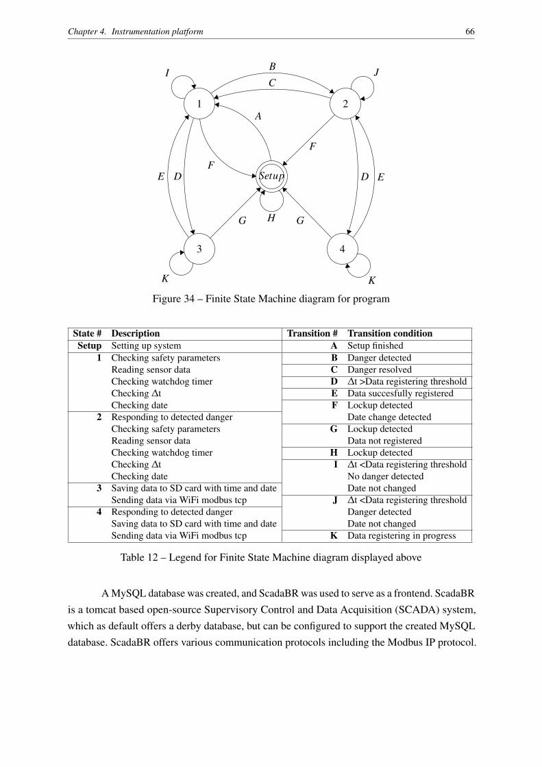
Chapter 4. Instrumentation platform 66
Setup
43
21
G G
F
F
A
E E
B
C
D D
H
K K
I J
Figure 34 – Finite State Machine diagram for program
State # Description Transition # Transition conditionSetup Setting up system A Setup finished
1 Checking safety parameters B Danger detectedReading sensor data C Danger resolvedChecking watchdog timer D ∆t >Data registering thresholdChecking ∆t E Data succesfully registeredChecking date F Lockup detected
2 Responding to detected danger Date change detectedChecking safety parameters G Lockup detectedReading sensor data Data not registeredChecking watchdog timer H Lockup detectedChecking ∆t I ∆t <Data registering thresholdChecking date No danger detected
3 Saving data to SD card with time and date Date not changedSending data via WiFi modbus tcp J ∆t <Data registering threshold
4 Responding to detected danger Danger detectedSaving data to SD card with time and date Date not changedSending data via WiFi modbus tcp K Data registering in progress
Table 12 – Legend for Finite State Machine diagram displayed above
A MySQL database was created, and ScadaBR was used to serve as a frontend. ScadaBRis a tomcat based open-source Supervisory Control and Data Acquisition (SCADA) system,which as default offers a derby database, but can be configured to support the created MySQLdatabase. ScadaBR offers various communication protocols including the Modbus IP protocol.

Chapter 4. Instrumentation platform 67
Thus, if SacadBR is configured correctly, the data encapsulated in the Modbus IP protocoland sent by the instrumentation platform via WiFi, is then received by ScadaBR, saved inthe MySQL database, and presented to an observer on the tomcat web server. Another handyfeature of ScadaBR is that one can publish the received data to IoT websites. Thingspeak.comwas tested as IoT server, and if desired, the data could be publicly published on the internet,allowing anyone to observe the turbine’s functionality.
4.4 Prototypes and tests
After finishing the detailed design phase, a first prototype was made. This prototypewas a good first experience in making printed circuit boards (PCB). As outlined in the detaileddesign, it was equipped with an Arduino Mega 2560, a CC3000 WiFi shield, 3 inputs fortemperature sensors, 1 input for a water detection sensor, 2 inputs for rotational speed sensors,3 inputs for the x, y, and z axes of an accelerometer, three inputs for current sensors, 3 inputs forvoltage sensors, and a redundant analog input. Figure 69 shows the PCB design of prototypeversion 0.5. The sensors were tested and all functioning correctly.
Note that the safety actuating mechanical relays were not present on the first prototype.In the second prototype however, the relays were embedded in the PCB. The microcontroller,WiFi shield, and inputs remained unchanged. Figure 70 in appendix C shows the PCB designof prototype version 1.0. This prototype was installed in a metal instrumentation box (seefigure 35a)
The instrumentation box was mounted in such a way that a larger PCB could be installedto monitor all three turbines. Prototype V1.0 was tested on a turbine mounted on- and driven bya lathe as illustrated in figure 35b.

Chapter 4. Instrumentation platform 68
(a) The second instrumentation prototype in-stalled in the instrumentation box
(b) Turbine testing mounted on and drivenby a lathe
Figure 35 – Instrumentation platform testing on lathe
During the tests, various problems were discovered. One of the problems was that inno-load situations, the voltage surpassed 1000 V in some cases. Figure 36b shows the no-loadRMS AC-line voltage output at various rotational velocities. This problem was solved bydesigning a high-voltage, selective resolution, voltage divider with a zener diode, that limitsthe voltage on the analog input of the Arduino to 5 v (shown in figure 73 of appendix F).As mentioned in the previous subsection, it has a maximum rated voltage measurement of1000VDC with a relay to double the resolution at voltages lower than 500VDC.
Another issue, was the flexible coupling, between the rotor and the generator, whichdestroyed the proximity/RPM sensor during the first tests, due to an unintentional-excessiveexpansion of the rubber coupling (see figure 36a). This was either due to an under dimensionedflexible coupling, or an abnormally high torque, generated by the lathe. The proximity sensorwas installed near this flexible coupling because it served as the cogwheel necessary to makethe velocity calculation possible, as described in the last subsection. The issue of the breakingproximity sensor was resolved by relocating the RPM sensor to a different area of the axle,where there is no expanding material and a purposely designed metal cogwheel.
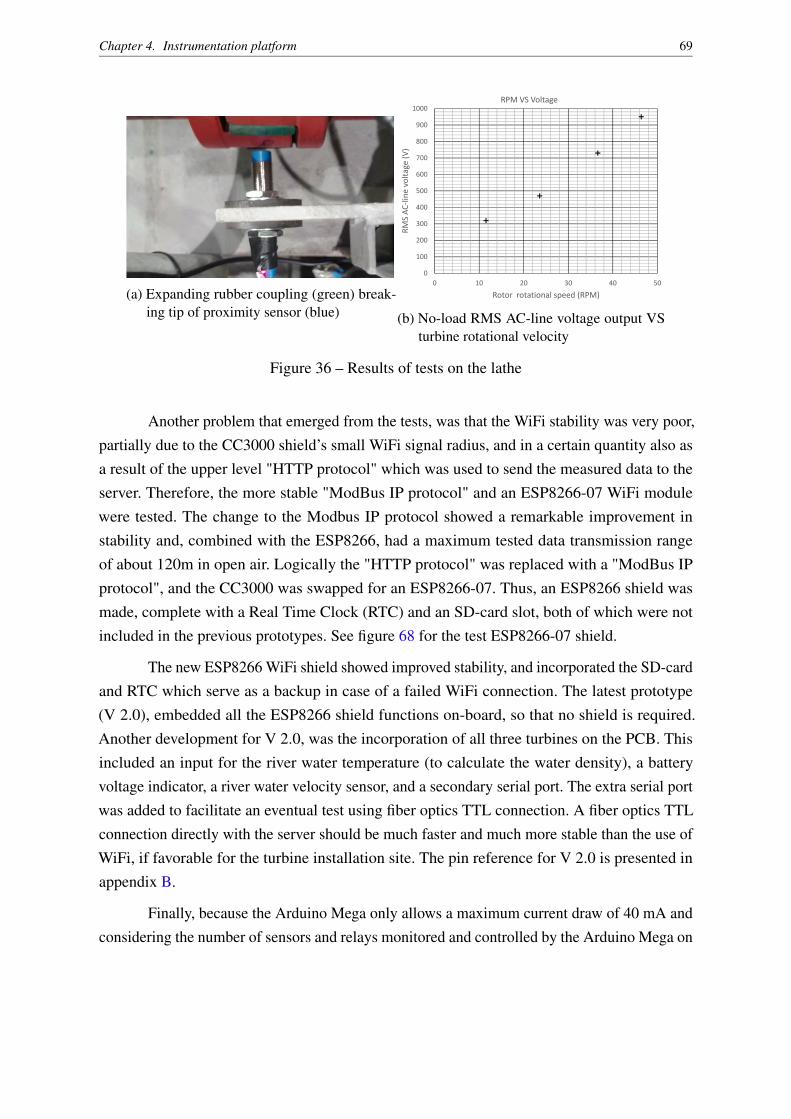
Chapter 4. Instrumentation platform 69
(a) Expanding rubber coupling (green) break-ing tip of proximity sensor (blue)
(b) No-load RMS AC-line voltage output VSturbine rotational velocity
Figure 36 – Results of tests on the lathe
Another problem that emerged from the tests, was that the WiFi stability was very poor,partially due to the CC3000 shield’s small WiFi signal radius, and in a certain quantity also asa result of the upper level "HTTP protocol" which was used to send the measured data to theserver. Therefore, the more stable "ModBus IP protocol" and an ESP8266-07 WiFi modulewere tested. The change to the Modbus IP protocol showed a remarkable improvement instability and, combined with the ESP8266, had a maximum tested data transmission rangeof about 120m in open air. Logically the "HTTP protocol" was replaced with a "ModBus IPprotocol", and the CC3000 was swapped for an ESP8266-07. Thus, an ESP8266 shield wasmade, complete with a Real Time Clock (RTC) and an SD-card slot, both of which were notincluded in the previous prototypes. See figure 68 for the test ESP8266-07 shield.
The new ESP8266 WiFi shield showed improved stability, and incorporated the SD-cardand RTC which serve as a backup in case of a failed WiFi connection. The latest prototype(V 2.0), embedded all the ESP8266 shield functions on-board, so that no shield is required.Another development for V 2.0, was the incorporation of all three turbines on the PCB. Thisincluded an input for the river water temperature (to calculate the water density), a batteryvoltage indicator, a river water velocity sensor, and a secondary serial port. The extra serial portwas added to facilitate an eventual test using fiber optics TTL connection. A fiber optics TTLconnection directly with the server should be much faster and much more stable than the use ofWiFi, if favorable for the turbine installation site. The pin reference for V 2.0 is presented inappendix B.
Finally, because the Arduino Mega only allows a maximum current draw of 40 mA andconsidering the number of sensors and relays monitored and controlled by the Arduino Mega on
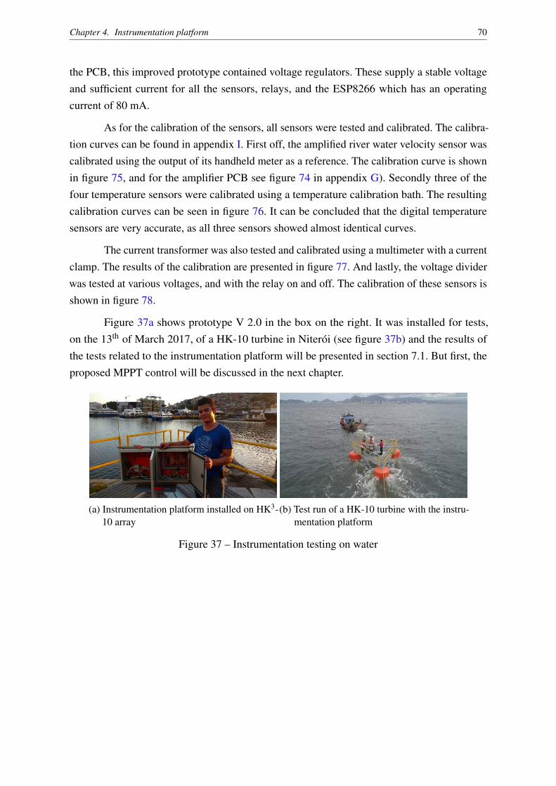
Chapter 4. Instrumentation platform 70
the PCB, this improved prototype contained voltage regulators. These supply a stable voltageand sufficient current for all the sensors, relays, and the ESP8266 which has an operatingcurrent of 80 mA.
As for the calibration of the sensors, all sensors were tested and calibrated. The calibra-tion curves can be found in appendix I. First off, the amplified river water velocity sensor wascalibrated using the output of its handheld meter as a reference. The calibration curve is shownin figure 75, and for the amplifier PCB see figure 74 in appendix G). Secondly three of thefour temperature sensors were calibrated using a temperature calibration bath. The resultingcalibration curves can be seen in figure 76. It can be concluded that the digital temperaturesensors are very accurate, as all three sensors showed almost identical curves.
The current transformer was also tested and calibrated using a multimeter with a currentclamp. The results of the calibration are presented in figure 77. And lastly, the voltage dividerwas tested at various voltages, and with the relay on and off. The calibration of these sensors isshown in figure 78.
Figure 37a shows prototype V 2.0 in the box on the right. It was installed for tests,on the 13th of March 2017, of a HK-10 turbine in Niterói (see figure 37b) and the results ofthe tests related to the instrumentation platform will be presented in section 7.1. But first, theproposed MPPT control will be discussed in the next chapter.
(a) Instrumentation platform installed on HK3-10 array
(b) Test run of a HK-10 turbine with the instru-mentation platform
Figure 37 – Instrumentation testing on water
71
5 Control of hydrokinetic turbines
As introduced in section 2.3, this chapter will be dedicated to discussing variousapproaches for the optimal control of variable speed - fixed pitch turbines starting with themore conventional variable speed - fixed pitch turbine control strategies.
5.1 Non-MPPT variable speed - fixed pitch turbine control
One approach for optimal control of variable speed - fixed pitch turbines uses a setpointfrom the water velocity information to control the rotational speed of the rotor shaft. Thisapproach is only suitable if the optimal value of the tip speed ratio (λopt), and the current rivervelocity (U∞) are known. The optimal rotational velocity (ωopt) is that where:
λ(t) = λopt ⇒ ωopt(t) =λopt
rU∞(t) (5.1)
A drawback to this approach is that λopt should be known, which implies that a mappingof the CP - λ curve must be done.
Another approach for controlling variable speed - fixed pitch turbines is using a setpointfrom the shaft rotational speed information to actively control the turbine. This method is onlysuitable if λopt and the maximum power coefficient (Cp max = CP(λopt)) are known, whichagain implies that a mapping of the CP - λ curve must be done. By combining equations 2.1,2.3, and 2.4 follows:
P =12
CPρπr2U3∞ =
12
CP
λ3 ρπrω3 (5.2)
Inserting λ = λopt and CP =CPmax in equation 5.2 one obtains the power reference:
Popt = Pre f = K ·ω3opt (5.3)
Using equations 2.1, 2.4, and 5.1 we can deduce that:
K =12
CPmax
λ3opt
ρπr5 (5.4)
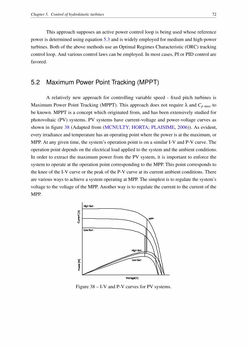
Chapter 5. Control of hydrokinetic turbines 72
This approach supposes an active power control loop is being used whose referencepower is determined using equation 5.3 and is widely employed for medium and high-powerturbines. Both of the above methods use an Optimal Regimes Characteristic (ORC) trackingcontrol loop. And various control laws can be employed. In most cases, PI or PID control arefavored.
5.2 Maximum Power Point Tracking (MPPT)
A relatively new approach for controlling variable speed - fixed pitch turbines isMaximum Power Point Tracking (MPPT). This approach does not require λ and Cp max tobe known. MPPT is a concept which originated from, and has been extensively studied forphotovoltaic (PV) systems. PV systems have current-voltage and power-voltage curves asshown in figure 38 (Adapted from (MCNULTY; HORTA; PLAISIME, 2006)). As evident,every irradiance and temperature has an operating point where the power is at the maximum, orMPP. At any given time, the system’s operation point is on a similar I-V and P-V curve. Theoperation point depends on the electrical load applied to the system and the ambient conditions.In order to extract the maximum power from the PV system, it is important to enforce thesystem to operate at the operation point corresponding to the MPP. This point corresponds tothe knee of the I-V curve or the peak of the P-V curve at its current ambient conditions. Thereare various ways to achieve a system operating at MPP. The simplest is to regulate the system’svoltage to the voltage of the MPP. Another way is to regulate the current to the current of theMPP.
Figure 38 – I-V and P-V curves for PV systems.
Chapter 5. Control of hydrokinetic turbines 73
Given that the I-V and P-V curves depend on the ambient conditions, such as irradianceand temperature, the MPP will fluctuate with changing ambient conditions. In order to regulatethe system’s voltage or current to the voltage or current of the MPP, the maximum power pointshould be tracked. This process is called Maximum Power Point Tracking (MPPT). MPPTdevices track the MPP using one or more MPPT algorithms.
The two main groups of MPPT algorithms are the indirect MPPT and the direct, orhill climb MPPT method. The first one uses simple measurements to make assumptions andperiodic estimations of the MPPT. The direct MPPT methods, measure current, voltage, orpower and have a faster response than the indirect methods.
5.2.1 MPPT for PV systems
As stated above, the concept of MPPT originated from PV systems. This section willdiscuss a few algorithms for PV systems, starting with the indirect MPPT algorithms.
One of the indirect MPPT algorithms is the Fixed voltage method. This method isbased on adjusting the operational voltage of the system only according to the season. Thismethod is less efficient, as there are irradiance fluctuations independent of the season on adaily basis. Another indirect MPPT method is the Fractional open circuit voltage method.This method exploits the fact that the MPP is located at a certain distance from the opencircuit voltage. Therefore the operation voltage is regulated to VMPP = k×VOC. Where k is aconstant smaller than 1 (in general 0.7-0.8) and approximates the MPP, as it is a ratio betweenMPP voltage (VMPP) and the open circuit voltage (VOC). This ratio diverges very little withchanging irradiance. A disadvantage of this method is that the load on the PV system has tobe temporarily and repeatedly disconnected in order to measure the VOC, resulting in a loss ofpower extraction.
The more involved of the two main MPPT algorithms, the direct MPPT algorithms,measure current, voltage, or power and have a faster response than the indirect methods.
One of the direct MPPT methods is the Perturb and observe method. This methodexploits the fact that the P-V curve is always increasing on the left side of the MPP, anddecreasing on the right side of the MPP. Changing the load on the system will result in anincrease or decrease in the power. Periodically increasing or decreasing the load in the directionof an increasing power, results in a high power extraction, but never the maximum, becausethe algorithm can not remain on the MPP, but hovers around it. Another disadvantage of thismethod is that it can fail to converge in rapidly fluctuating ambient conditions.
Chapter 5. Control of hydrokinetic turbines 74
The incremental conductance method is another hill climb MPPT algorithm. Thismethod exploits the fact that the MPP corresponds to the knee of the I-V curve and that theslope of the P-V curve is zero at the MPP. Therefore, dP
dV can be rewritten as:
dPdV
=d(I×V )
dV= I +
V ×dIdV
And since the slope is dPdV = 0, ∆I
∆V =− IV . As the conductance of the system is I
V , the system’soperation point relative to the MPP is:
∆I∆V
=− IV
at MPP
∆I∆V
>− IV
to the le f t o f MPP
∆I∆V
<− IV
to the right o f MPP
At every iteration the algorithm imposes a voltage to the system, measures the resulting incre-mental change in conductance, compares it with the instantaneous conductance, and therebydiscovering the operation point relative to the MPP. This method can be more efficient thanthe previous algorithms because it can remain on the MPP, and does not need to hover aroundit in steady state conditions. High sampling frequencies make this method less susceptible tofluctuating ambient conditions. The drawbacks of this method are that in highly fluctuating,and partial shading conditions the algorithm is unlikely to converge towards the MPP. Nganand Tan (2011) discusses an algorithm suitable for the aforementioned conditions.
5.2.2 MPPT for wind energy systems
In the last decade the literature concerning MPPT for wind energy systems has advanced.Various MPPT control methods have been described, simulated, and applied to wind energyconversion systems. MPPT has been implemented in various wind turbines (HUA; GENG,2006; HAQUE; NEGNEVITSKY; MUTTAQI, 2010; AUBRÉE et al., 2016), and has recentlyalso been applied to HKT’s (ZHOU, 2012) (MOFEI, 2014). HKT’s and wind turbines basicallyhave the same working principle. What differentiates the hydro from the wind turbine is thatthe hydro kinetic turbine; extracts power from a different fluid, has lower tip speed ratio ranges,cavitation limits and is exposed to a more harsh environment (GINTER; PIEPER, 2009). Thereis a large amount of literature describing the control of wind turbines and relatively few paperson the control of hydro-kinetic turbines. Munteanu et al. (2008) describes various conventionalways of controlling wind turbines including MPPT.
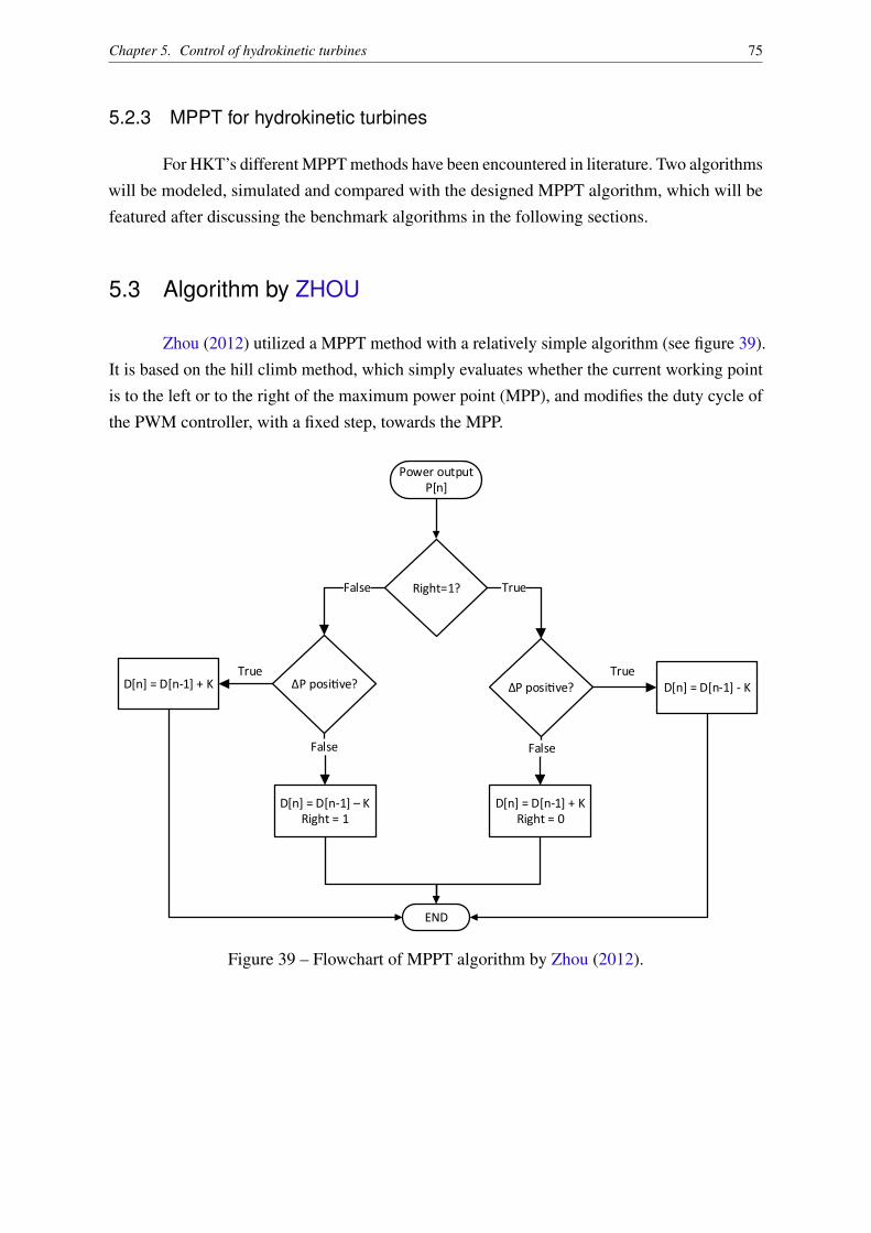
Chapter 5. Control of hydrokinetic turbines 75
5.2.3 MPPT for hydrokinetic turbines
For HKT’s different MPPT methods have been encountered in literature. Two algorithmswill be modeled, simulated and compared with the designed MPPT algorithm, which will befeatured after discussing the benchmark algorithms in the following sections.
5.3 Algorithm by ZHOU
Zhou (2012) utilized a MPPT method with a relatively simple algorithm (see figure 39).It is based on the hill climb method, which simply evaluates whether the current working pointis to the left or to the right of the maximum power point (MPP), and modifies the duty cycle ofthe PWM controller, with a fixed step, towards the MPP.
Power output P[n]
Right=1?
ΔP posive?D[n] = D[n-1] + K
False True
True
False False
D[n] = D[n-1] – KRight = 1
ΔP posive? D[n] = D[n-1] - KTrue
D[n] = D[n-1] + KRight = 0
END
Figure 39 – Flowchart of MPPT algorithm by Zhou (2012).
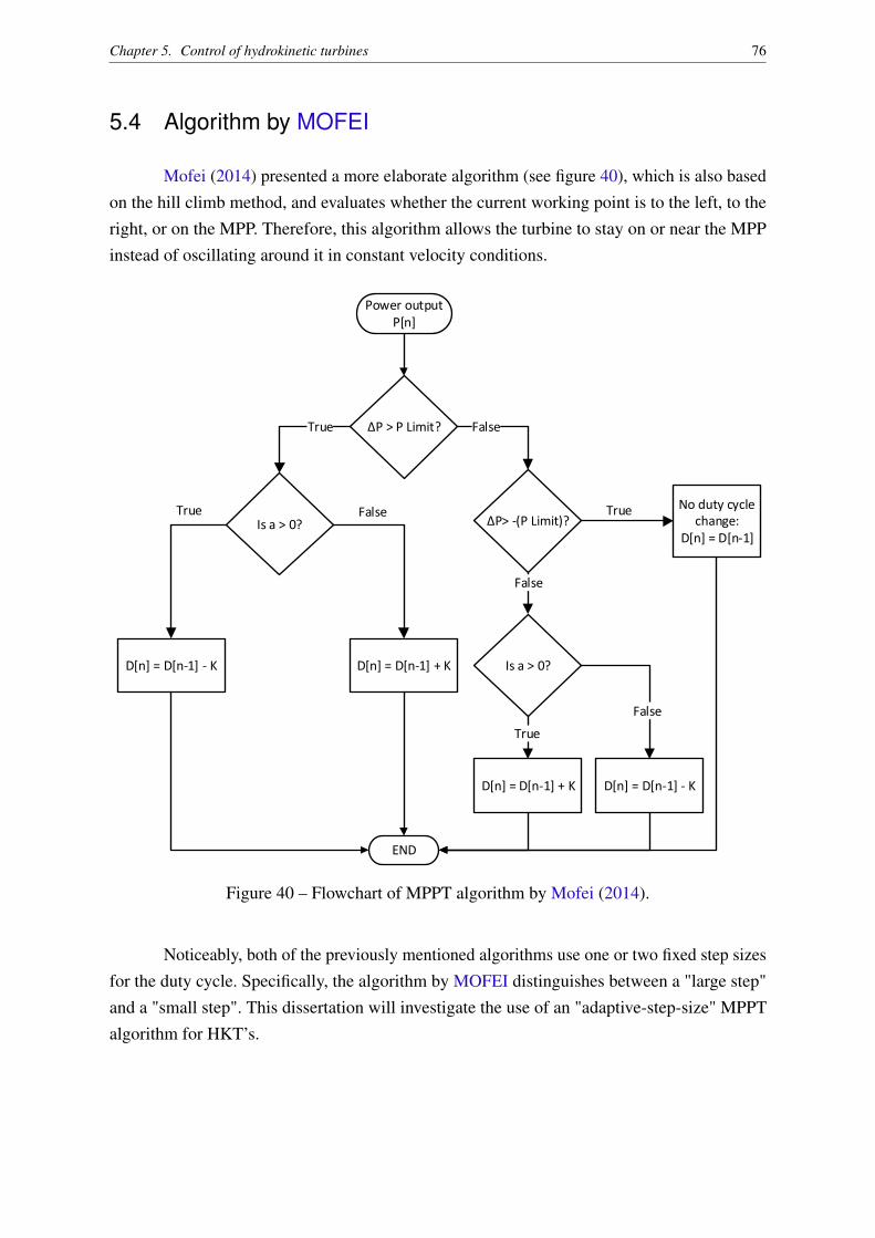
Chapter 5. Control of hydrokinetic turbines 76
5.4 Algorithm by MOFEI
Mofei (2014) presented a more elaborate algorithm (see figure 40), which is also basedon the hill climb method, and evaluates whether the current working point is to the left, to theright, or on the MPP. Therefore, this algorithm allows the turbine to stay on or near the MPPinstead of oscillating around it in constant velocity conditions.
Power output P[n]
ΔP > P Limit?
Is a > 0?
D[n] = D[n-1] - K
True False
True False
END
ΔP> -(P Limit)?
Is a > 0?
False
D[n] = D[n-1] + K
No duty cycle change:
D[n] = D[n-1]
True
True
D[n] = D[n-1] - K
False
D[n] = D[n-1] + K
Figure 40 – Flowchart of MPPT algorithm by Mofei (2014).
Noticeably, both of the previously mentioned algorithms use one or two fixed step sizesfor the duty cycle. Specifically, the algorithm by MOFEI distinguishes between a "large step"and a "small step". This dissertation will investigate the use of an "adaptive-step-size" MPPTalgorithm for HKT’s.
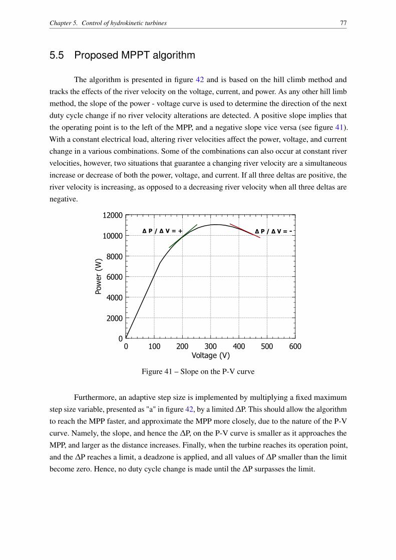
Chapter 5. Control of hydrokinetic turbines 77
5.5 Proposed MPPT algorithm
The algorithm is presented in figure 42 and is based on the hill climb method andtracks the effects of the river velocity on the voltage, current, and power. As any other hill limbmethod, the slope of the power - voltage curve is used to determine the direction of the nextduty cycle change if no river velocity alterations are detected. A positive slope implies thatthe operating point is to the left of the MPP, and a negative slope vice versa (see figure 41).With a constant electrical load, altering river velocities affect the power, voltage, and currentchange in a various combinations. Some of the combinations can also occur at constant rivervelocities, however, two situations that guarantee a changing river velocity are a simultaneousincrease or decrease of both the power, voltage, and current. If all three deltas are positive, theriver velocity is increasing, as opposed to a decreasing river velocity when all three deltas arenegative.
Pow
er
(W)
Voltage (V)0 100 200 300 400 500 600
0
2000
4000
6000
8000
10000
12000
Δ P / Δ V = + Δ P / Δ V = -
Figure 41 – Slope on the P-V curve
Furthermore, an adaptive step size is implemented by multiplying a fixed maximumstep size variable, presented as "a" in figure 42, by a limited ∆P. This should allow the algorithmto reach the MPP faster, and approximate the MPP more closely, due to the nature of the P-Vcurve. Namely, the slope, and hence the ∆P, on the P-V curve is smaller as it approaches theMPP, and larger as the distance increases. Finally, when the turbine reaches its operation point,and the ∆P reaches a limit, a deadzone is applied, and all values of ∆P smaller than the limitbecome zero. Hence, no duty cycle change is made until the ∆P surpasses the limit.
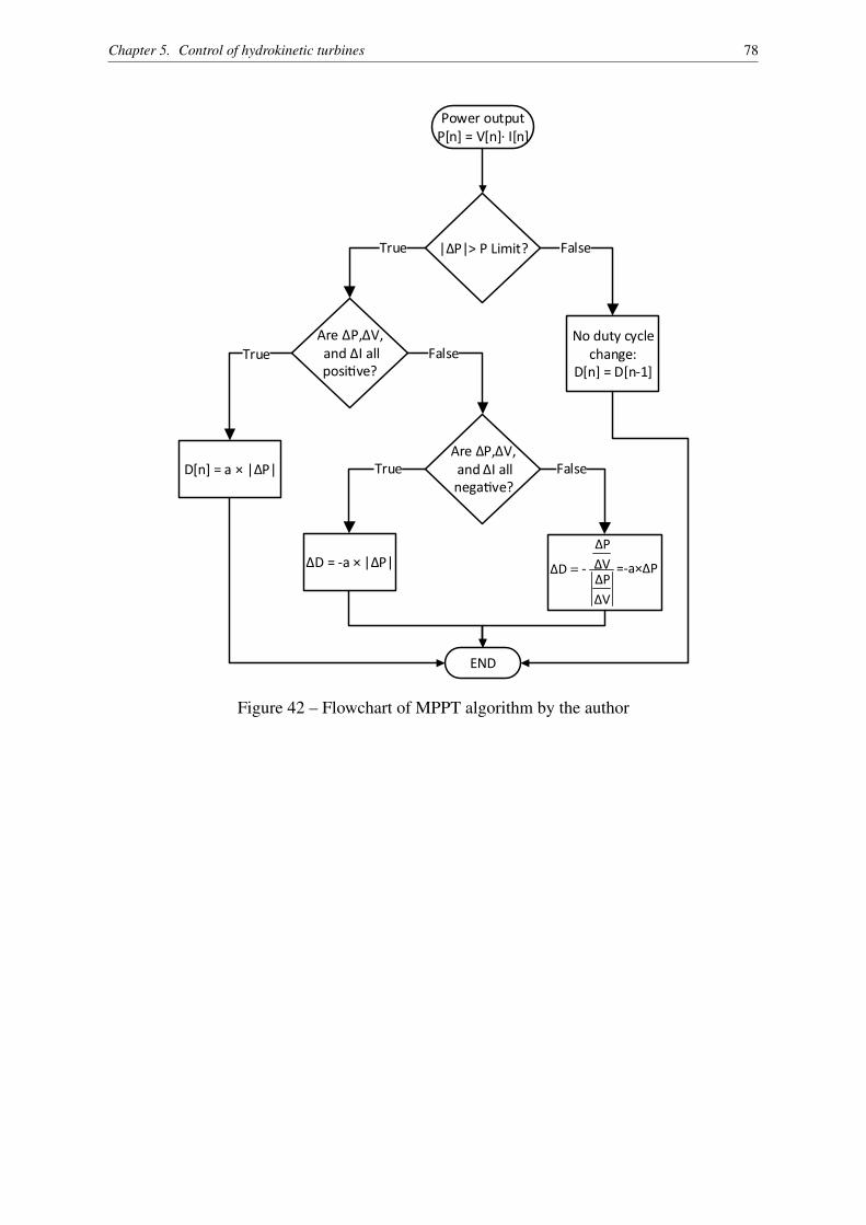
Chapter 5. Control of hydrokinetic turbines 78
Power output P[n] = V[n]· I[n]
|ΔP|> P Limit?
Are ΔP,ΔV, and ΔI all posive?
Are ΔP,ΔV, and ΔI all negave?
No duty cycle change:
D[n] = D[n-1]
D[n] = a × |ΔP|
ΔD = -a × |ΔP|
True False
True False
True False
=-a×ΔP
ΔVΔPΔVΔP
ΔD = -
END
Figure 42 – Flowchart of MPPT algorithm by the author
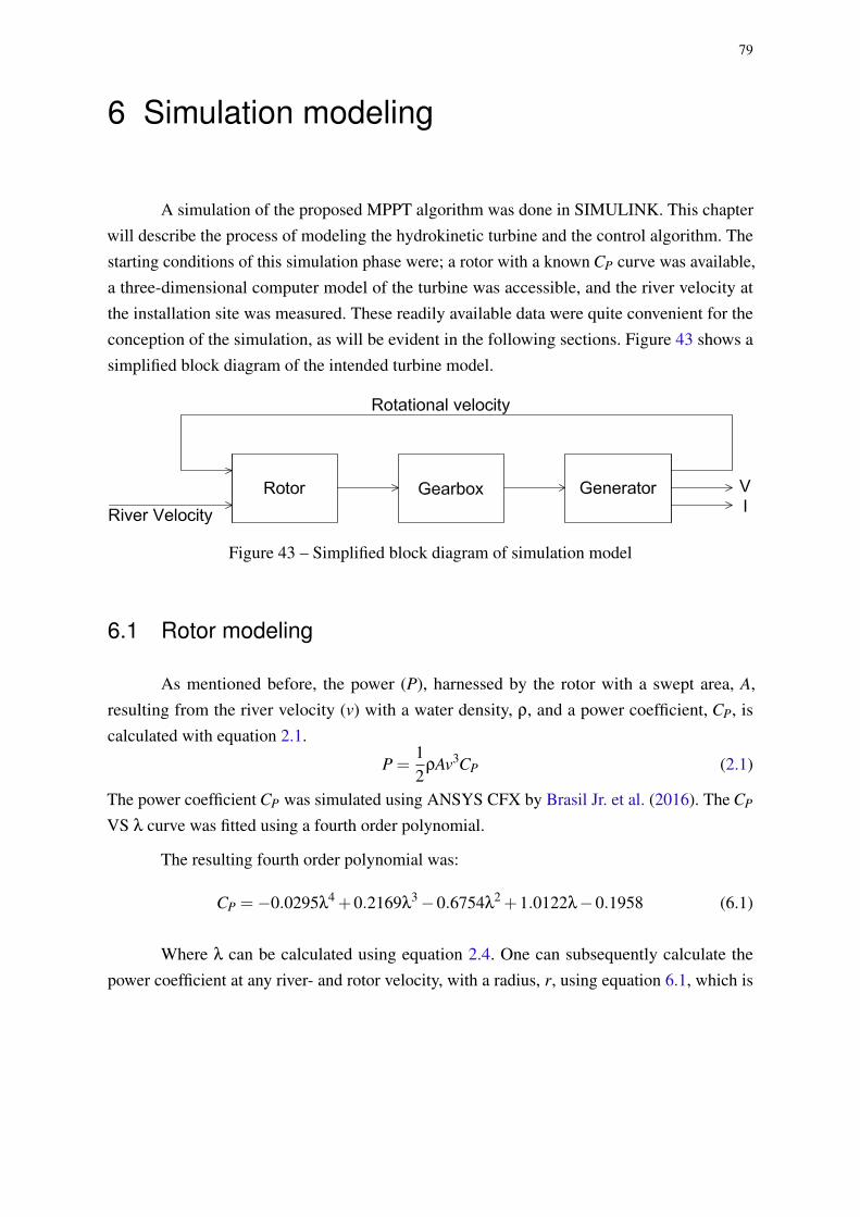
79
6 Simulation modeling
A simulation of the proposed MPPT algorithm was done in SIMULINK. This chapterwill describe the process of modeling the hydrokinetic turbine and the control algorithm. Thestarting conditions of this simulation phase were; a rotor with a known CP curve was available,a three-dimensional computer model of the turbine was accessible, and the river velocity atthe installation site was measured. These readily available data were quite convenient for theconception of the simulation, as will be evident in the following sections. Figure 43 shows asimplified block diagram of the intended turbine model.
Figure 43 – Simplified block diagram of simulation model
6.1 Rotor modeling
As mentioned before, the power (P), harnessed by the rotor with a swept area, A,resulting from the river velocity (v) with a water density, ρ, and a power coefficient, CP, iscalculated with equation 2.1.
P =12
ρAv3CP (2.1)
The power coefficient CP was simulated using ANSYS CFX by Brasil Jr. et al. (2016). The CP
VS λ curve was fitted using a fourth order polynomial.
The resulting fourth order polynomial was:
CP =−0.0295λ4 +0.2169λ
3−0.6754λ2 +1.0122λ−0.1958 (6.1)
Where λ can be calculated using equation 2.4. One can subsequently calculate thepower coefficient at any river- and rotor velocity, with a radius, r, using equation 6.1, which is
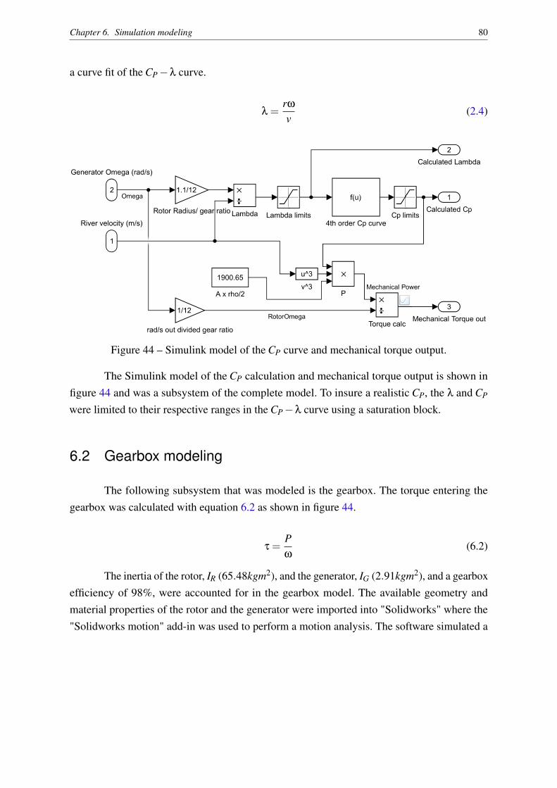
Chapter 6. Simulation modeling 80
a curve fit of the CP−λ curve.
λ =rω
v(2.4)
Figure 44 – Simulink model of the CP curve and mechanical torque output.
The Simulink model of the CP calculation and mechanical torque output is shown infigure 44 and was a subsystem of the complete model. To insure a realistic CP, the λ and CP
were limited to their respective ranges in the CP−λ curve using a saturation block.
6.2 Gearbox modeling
The following subsystem that was modeled is the gearbox. The torque entering thegearbox was calculated with equation 6.2 as shown in figure 44.
τ =Pω
(6.2)
The inertia of the rotor, IR (65.48kgm2), and the generator, IG (2.91kgm2), and a gearboxefficiency of 98%, were accounted for in the gearbox model. The available geometry andmaterial properties of the rotor and the generator were imported into "Solidworks" where the"Solidworks motion" add-in was used to perform a motion analysis. The software simulated a
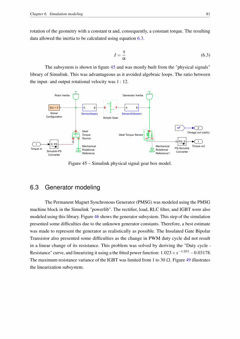
Chapter 6. Simulation modeling 81
rotation of the geometry with a constant α and, consequently, a constant torque. The resultingdata allowed the inertia to be calculated using equation 6.3.
I =τ
α(6.3)
The subsystem is shown in figure 45 and was mostly built from the "physical signals"library of Simulink. This was advantageous as it avoided algebraic loops. The ratio betweenthe input- and output rotational velocity was 1 : 12.
B FFB
SimpleGear
RotorInertia GeneratorInertia
A B
Sensor(base)
A B
Sensor(follower)
RS C
RCS
IdealTorqueSource
MechanicalRotationalReference
S PS
Simulink-PSConverter
f(x)=0
SolverConfiguration
1Torquein
1Torqueout
2Omegaout(rad/s)
wF
MechanicalRotationalReference1
RCTT C
R
IdealTorqueSensor
SPS
PS-SimulinkConverter
Figure 45 – Simulink physical signal gear box model.
6.3 Generator modeling
The Permanent Magnet Synchronous Generator (PMSG) was modeled using the PMSGmachine block in the Simulink "powerlib". The rectifier, load, RLC filter, and IGBT were alsomodeled using this library. Figure 46 shows the generator subsystem. This step of the simulationpresented some difficulties due to the unknown generator constants. Therefore, a best estimatewas made to represent the generator as realistically as possible. The Insulated Gate BipolarTransistor also presented some difficulties as the change in PWM duty cycle did not resultin a linear change of its resistance. This problem was solved by deriving the "Duty cycle -Resistance" curve, and linearizing it using a the fitted power function: 1.023×x−1.031−0.03178.The maximum resistance variance of the IGBT was limited from 1 to 30Ω. Figure 49 illustratesthe linearization subsystem.
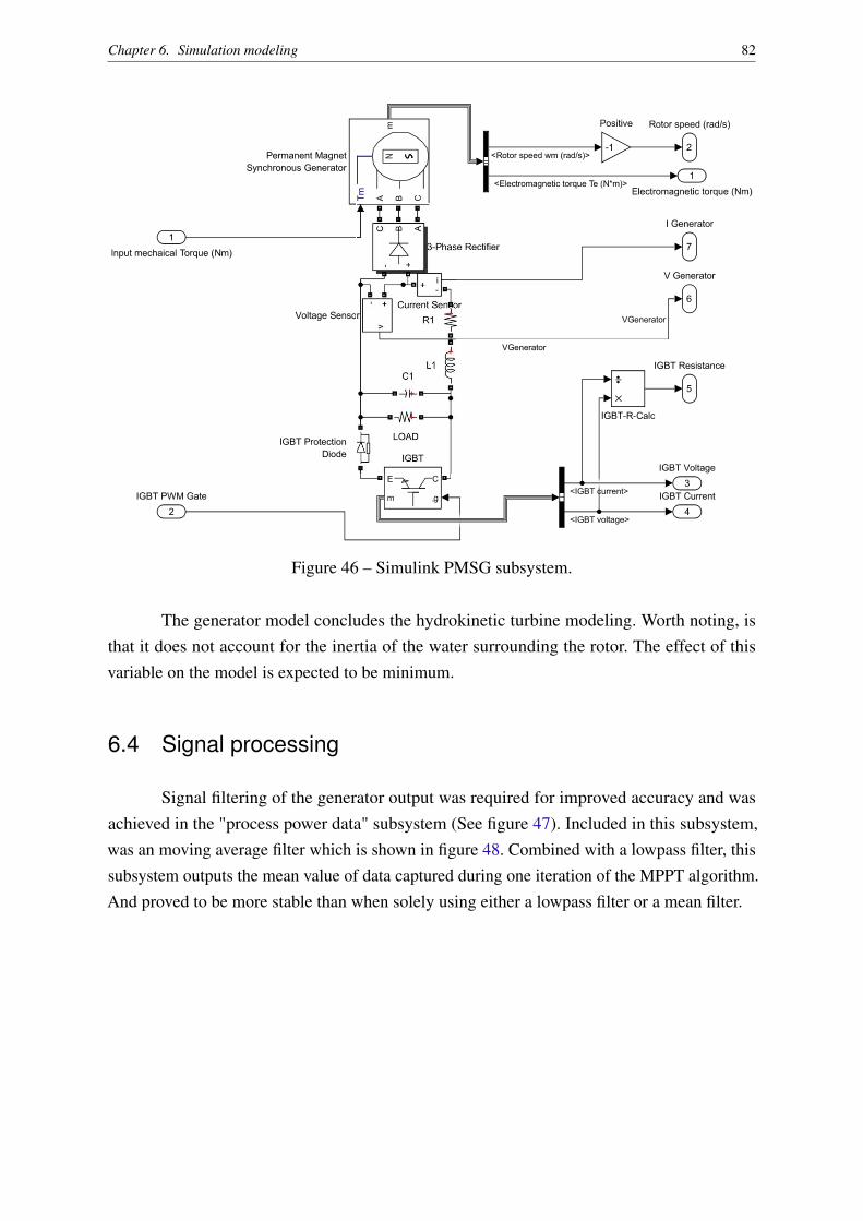
Chapter 6. Simulation modeling 82
Figure 46 – Simulink PMSG subsystem.
The generator model concludes the hydrokinetic turbine modeling. Worth noting, isthat it does not account for the inertia of the water surrounding the rotor. The effect of thisvariable on the model is expected to be minimum.
6.4 Signal processing
Signal filtering of the generator output was required for improved accuracy and wasachieved in the "process power data" subsystem (See figure 47). Included in this subsystem,was an moving average filter which is shown in figure 48. Combined with a lowpass filter, thissubsystem outputs the mean value of data captured during one iteration of the MPPT algorithm.And proved to be more stable than when solely using either a lowpass filter or a mean filter.
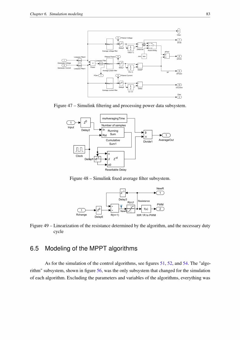
Chapter 6. Simulation modeling 83
Figure 47 – Simulink filtering and processing power data subsystem.
Figure 48 – Simulink fixed average filter subsystem.
Figure 49 – Linearization of the resistance determined by the algorithm, and the necessary dutycycle
6.5 Modeling of the MPPT algorithms
As for the simulation of the control algorithms, see figures 51, 52, and 54. The "algo-rithm" subsystem, shown in figure 56, was the only subsystem that changed for the simulationof each algorithm. Excluding the parameters and variables of the algorithms, everything was
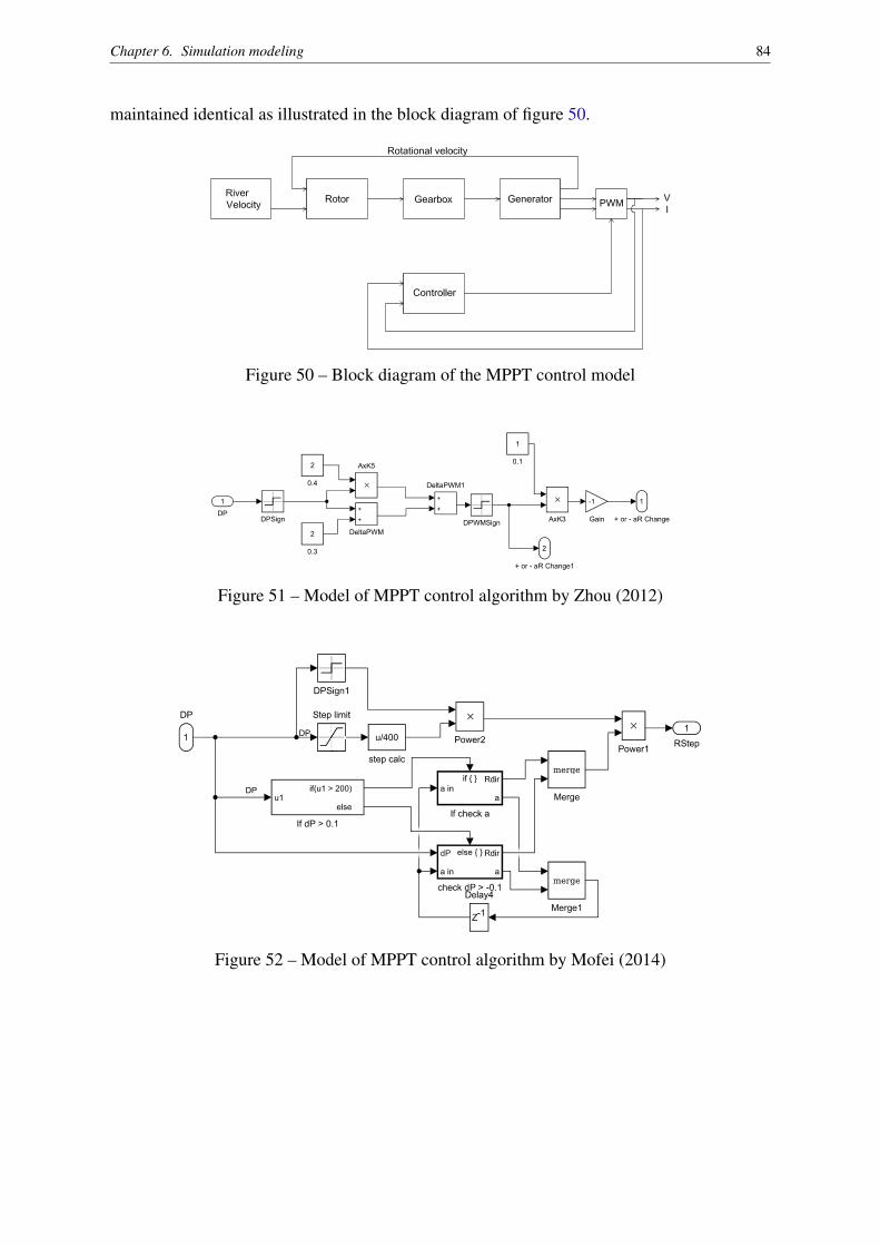
Chapter 6. Simulation modeling 84
maintained identical as illustrated in the block diagram of figure 50.
Figure 50 – Block diagram of the MPPT control model
Figure 51 – Model of MPPT control algorithm by Zhou (2012)
Figure 52 – Model of MPPT control algorithm by Mofei (2014)
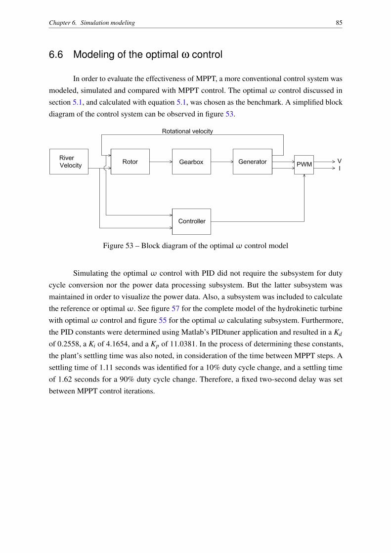
Chapter 6. Simulation modeling 85
6.6 Modeling of the optimal ω control
In order to evaluate the effectiveness of MPPT, a more conventional control system wasmodeled, simulated and compared with MPPT control. The optimal ω control discussed insection 5.1, and calculated with equation 5.1, was chosen as the benchmark. A simplified blockdiagram of the control system can be observed in figure 53.
Figure 53 – Block diagram of the optimalω control model
Simulating the optimal ω control with PID did not require the subsystem for dutycycle conversion nor the power data processing subsystem. But the latter subsystem wasmaintained in order to visualize the power data. Also, a subsystem was included to calculatethe reference or optimalω. See figure 57 for the complete model of the hydrokinetic turbinewith optimalω control and figure 55 for the optimalω calculating subsystem. Furthermore,the PID constants were determined using Matlab’s PIDtuner application and resulted in a Kd
of 0.2558, a Ki of 4.1654, and a Kp of 11.0381. In the process of determining these constants,the plant’s settling time was also noted, in consideration of the time between MPPT steps. Asettling time of 1.11 seconds was identified for a 10% duty cycle change, and a settling timeof 1.62 seconds for a 90% duty cycle change. Therefore, a fixed two-second delay was setbetween MPPT control iterations.
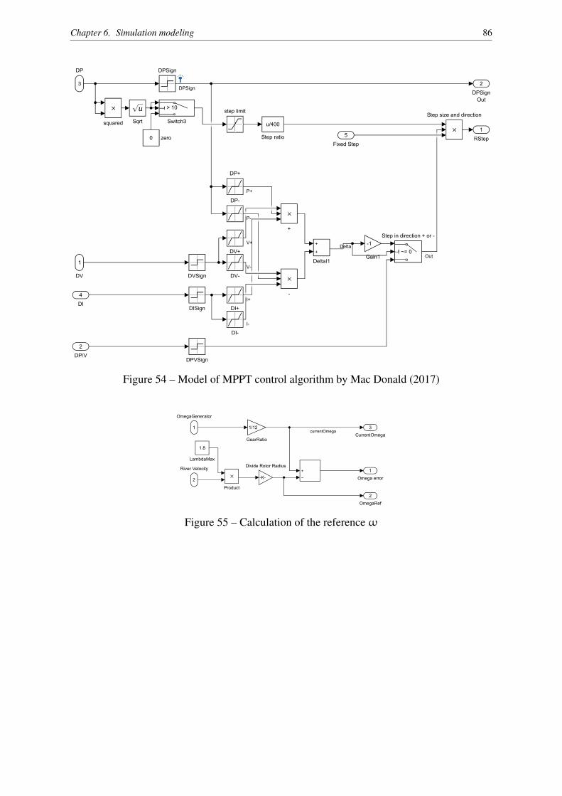
Chapter 6. Simulation modeling 86
Figure 54 – Model of MPPT control algorithm by Mac Donald (2017)
Figure 55 – Calculation of the referenceω
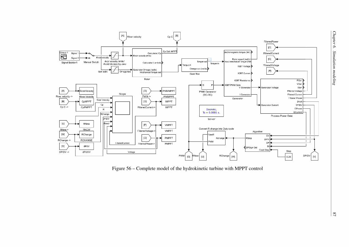
Chapter
6.Sim
ulationm
odeling87
Figure 56 – Complete model of the hydrokinetic turbine with MPPT control
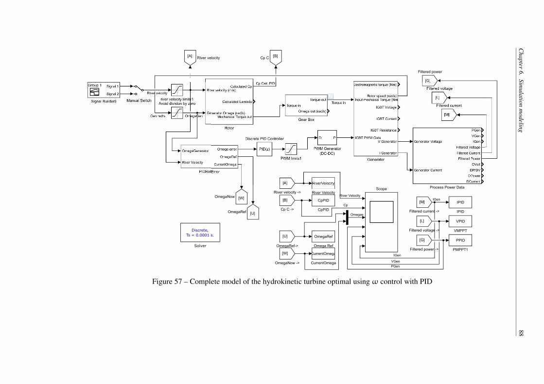
Chapter
6.Sim
ulationm
odeling88
Figure 57 – Complete model of the hydrokinetic turbine optimal usingω control with PID

89
7 Results
7.1 Instrumentation results
The results of the instrumentation platform are presented here, and will discuss afield test of a HK-10 turbine. Two test runs conducted on the 13th of March 2017 in Niteróirevealed various shortcomings and advantages of the instrumentation platform. The first wasthe robustness of the platform. During the trip to the test site, the "adjust" pin of an adjustablevoltage regulator was disconnected from the PCB, resulting in a 12V output where 3.3V wasdesired, causing the destruction of SD-cards and the WiFi module. Fortunately, the replacementof the defective parts was possible for they were locally available and inexpensive, which wasan objective for the design of the platform. Hence, it was repaired before the tests.
Another reliability issue was the malfunctioning amplifier. Unfortunately the amplifiercould not be repaired before the tests, thereby failing to read the incoming water velocity withthe instrumentation platform.
Regarding the sensors, a flaw was identified in the interfacing of the current and voltagesensors, as they were not suited nor calibrated for values lower than 10 A and lower than 110 Vrespectively. At lower values one could doubt the functionality of the sensors, their linearity,and the accuracy of the measurements (See Appendix I for the sensor calibrations).
Finally, the first test run revealed that the presentation of data was missing a filter, asthe values of the voltage fluctuated heavily, and the registration of data was missing the rawinput values and only registered treated data. Thanks to the flexibility of the system, the latterflaw was resolved quickly and in time for the second test run.
Positive results of the instrumentation platform were that the temperature, vibration,and rotational velocity sensors functioned without any faults or interference from electricalnoise, as will be show in the next paragraph. Furthermore, the Modbus TCP data transferoperated normally, the collected data was successfully saved to the SD-Card with time anddate, and the system proved to be adaptable.
The test data was collected in two test runs with a total time span of about 40 minutesand are shown in the subsequent figures. During the tests, the only form of control was a resistorbank that allowed the electrical resistance to be changed manually.
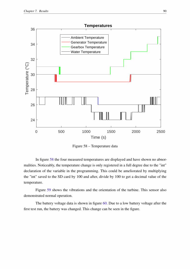
Chapter 7. Results 90
0 500 1000 1500 2000 2500
Time (s)
24
26
28
30
32
34
36T
empe
ratu
re (
°C)
Temperatures
Ambient TemperatureGenerator TemperatureGearbox TemperatureWater Temperature
Figure 58 – Temperature data
In figure 58 the four measured temperatures are displayed and have shown no abnor-malities. Noticeably, the temperature change is only registered in a full degree due to the "int"declaration of the variable in the programming. This could be ameliorated by multiplyingthe "int" saved to the SD card by 100 and after, divide by 100 to get a decimal value of thetemperature.
Figure 59 shows the vibrations and the orientation of the turbine. This sensor alsodemonstrated normal operation.
The battery voltage data is shown in figure 60. Due to a low battery voltage after thefirst test run, the battery was changed. This change can be seen in the figure.
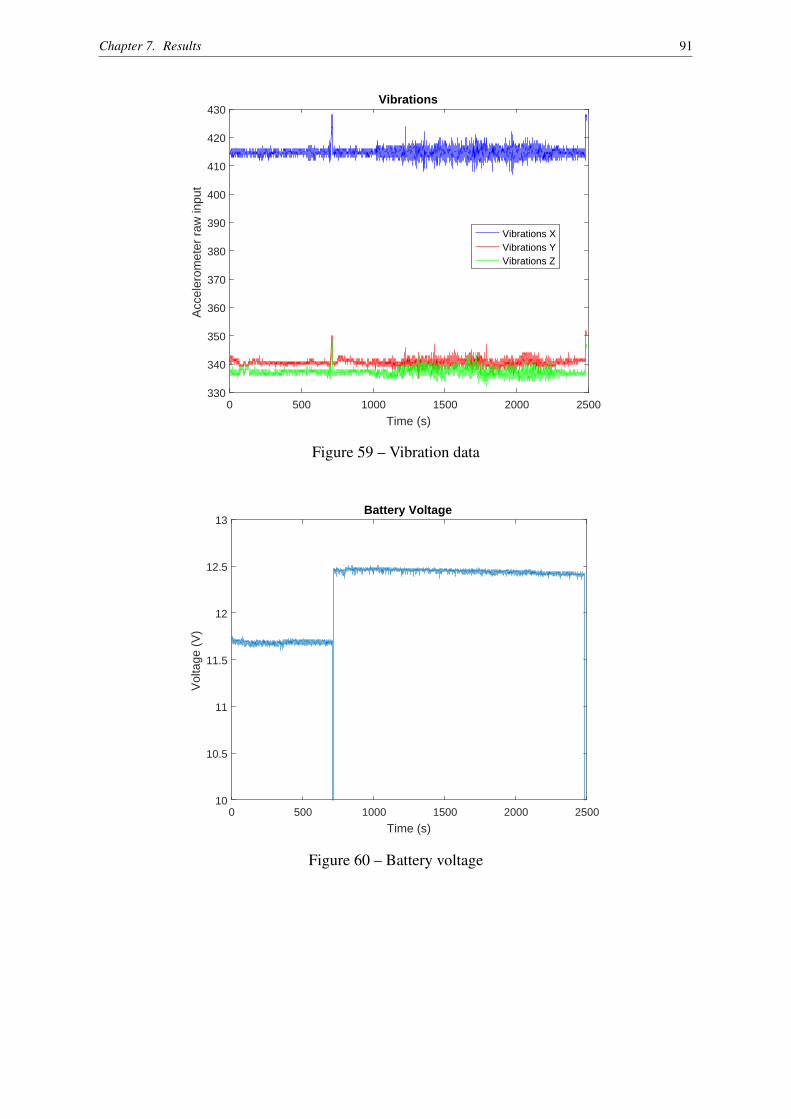
Chapter 7. Results 91
0 500 1000 1500 2000 2500
Time (s)
330
340
350
360
370
380
390
400
410
420
430
Acc
eler
omet
er r
aw in
put
Vibrations
Vibrations XVibrations YVibrations Z
Figure 59 – Vibration data
0 500 1000 1500 2000 2500
Time (s)
10
10.5
11
11.5
12
12.5
13
Vol
tage
(V
)
Battery Voltage
Figure 60 – Battery voltage
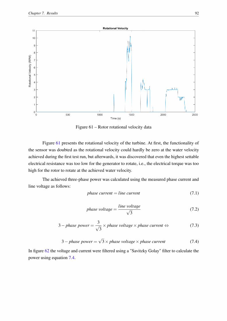
Chapter 7. Results 92
Figure 61 – Rotor rotational velocity data
Figure 61 presents the rotational velocity of the turbine. At first, the functionality ofthe sensor was doubted as the rotational velocity could hardly be zero at the water velocityachieved during the first test run, but afterwards, it was discovered that even the highest settableelectrical resistance was too low for the generator to rotate, i.e., the electrical torque was toohigh for the rotor to rotate at the achieved water velocity.
The achieved three-phase power was calculated using the measured phase current andline voltage as follows:
phase current = line current (7.1)
phase voltage =line voltage√
3(7.2)
3− phase power =3√3× phase voltage× phase current⇔ (7.3)
3− phase power =√
3× phase voltage× phase current (7.4)
In figure 62 the voltage and current were filtered using a "Savitzky Golay" filter to calculate thepower using equation 7.4.
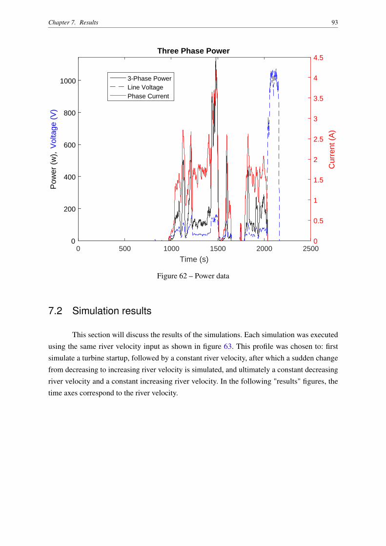
Chapter 7. Results 93
0 500 1000 1500 2000 2500
Time (s)
0
200
400
600
800
1000
Pow
er (
w),
Vol
tage
(V
)
0
0.5
1
1.5
2
2.5
3
3.5
4
4.5
Cur
rent
(A
)
Three Phase Power
3-Phase PowerLine VoltagePhase Current
Figure 62 – Power data
7.2 Simulation results
This section will discuss the results of the simulations. Each simulation was executedusing the same river velocity input as shown in figure 63. This profile was chosen to: firstsimulate a turbine startup, followed by a constant river velocity, after which a sudden changefrom decreasing to increasing river velocity is simulated, and ultimately a constant decreasingriver velocity and a constant increasing river velocity. In the following "results" figures, thetime axes correspond to the river velocity.
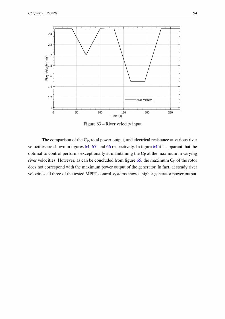
Chapter 7. Results 94
Riv
er
Velo
city
(m
/s)
Time (s)
0 50 100 150 200 250
1
1.2
1.4
1.6
1.8
2
2.2
2.4
River Velocity
Figure 63 – River velocity input
The comparison of the CP, total power output, and electrical resistance at various rivervelocities are shown in figures 64, 65, and 66 respectively. In figure 64 it is apparent that theoptimal ω control performs exceptionally at maintaining the CP at the maximum in varyingriver velocities. However, as can be concluded from figure 65, the maximum CP of the rotordoes not correspond with the maximum power output of the generator. In fact, at steady rivervelocities all three of the tested MPPT control systems show a higher generator power output.
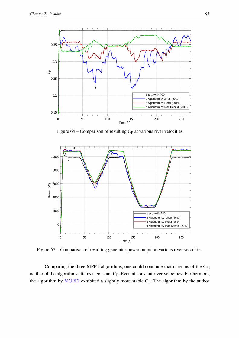
Chapter 7. Results 95
Cp
Time (s)0 50 100 150 200 250
0.15
0.2
0.25
0.3
0.35
1 ωOpt with PID
2 Algorithm by Zhou (2012)
3 Algorithm by Mofei (2014)
4 Algorithm by Mac Donald (2017)
1
2
3
4
Figure 64 – Comparison of resulting CP at various river velocities
Pow
er
(W)
Time (s)0 50 100 150 200 250
0
2000
4000
6000
8000
10000
1 ωOpt with PID
2 Algorithm bu Zhou (2012)
3 Algorithm by Mofei (2014)
4 Algorithm by Mac Donald (2017)
1
24
3
Figure 65 – Comparison of resulting generator power output at various river velocities
Comparing the three MPPT algorithms, one could conclude that in terms of the CP,neither of the algorithms attains a constant CP. Even at constant river velocities. Furthermore,the algorithm by MOFEI exhibited a slightly more stable CP. The algorithm by the author
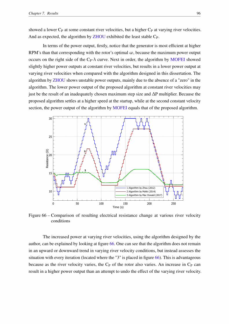
Chapter 7. Results 96
showed a lower CP at some constant river velocities, but a higher CP at varying river velocities.And as expected, the algorithm by ZHOU exhibited the least stable CP.
In terms of the power output, firstly, notice that the generator is most efficient at higherRPM’s than that corresponding with the rotor’s optimalω, because the maximum power outputoccurs on the right side of the CP-λ curve. Next in order, the algorithm by MOFEI showedslightly higher power outputs at constant river velocities, but results in a lower power output atvarying river velocities when compared with the algorithm designed in this dissertation. Thealgorithm by ZHOU shows unstable power outputs, mainly due to the absence of a "zero" in thealgorithm. The lower power output of the proposed algorithm at constant river velocities mayjust be the result of an inadequately chosen maximum step size and ∆P multiplier. Because theproposed algorithm settles at a higher speed at the startup, while at the second constant velocitysection, the power output of the algorithm by MOFEI equals that of the proposed algorithm.
Resi
stance
(Ω
)
Time (s)0 50 100 150 200 250
10
15
20
25
30
1 Algorithm by Zhou (2012)
2 Algorithm by Mofei (2014)
3 Algorithm by Mac Donald (2017)
1
2
3
Figure 66 – Comparison of resulting electrical resistance change at various river velocityconditions
The increased power at varying river velocities, using the algorithm designed by theauthor, can be explained by looking at figure 66. One can see that the algorithm does not remainin an upward or downward trend in varying river velocity conditions, but instead assesses thesituation with every iteration (located where the "3" is placed in figure 66). This is advantageousbecause as the river velocity varies, the CP of the rotor also varies. An increase in CP canresult in a higher power output than an attempt to undo the effect of the varying river velocity.

Chapter 7. Results 97
For example, in a decreasing river velocity situation, it can be more favorable to decreasethe turbine’s rotational velocity even more than it is already being decreased as result of theriver velocity, because the additional decrease increases the rotor’s CP, and subsequently thegenerator’s input torque. The other algorithms remain in an upward or downward trend untila certain condition is met, resulting in decreased CP values and notice that the algorithm byZHOU even reached the IGBT’s 30 Ohm limit.

98
8 Conclusions
8.1 Instrumentation conclusions
The conception goal of the instrumentation was creating a platform that facilitatesresearch on wind- and hydrokinetic turbines, with the HK-10 turbine as a specific application.Low cost and flexibility, were the main reasons for developing such a platform instead ofpurchasing a similar product.
Using the methodology detailed in chapter 4, the product’s architecture was defined,and various prototypes were produced, tested, and analyzed for improvements. The latestprototype proved to lack robustness, more accurate voltage and current sensors, a filtered datapresentation, and a more detailed data registering system. Nevertheless, prototypes by definitionare used to identify faults, and fortunately it did manage to measure the turbine’s power outputand functionality to a certain extent in field tests.
With low cost as a main objective, the robustness of the platform and the accuracy ofsome sensors showed to be less than desired, but the instrumentation platform has proven itsflexibility and low cost advantages during the field tests.
8.1.1 Future work
From the conclusions drawn in this chapter, emerges the necessity to:
• Increase robustness of the platform using low cost components such as:diodes to avoid reversed polarity,LED’s to quickly confirm or disprove the functionality of components,implementation of fuses to insure safe operation conditions,the enlarging of PCB soldering pads for critical components such as voltage regula-
tors,and varistors to avoid undesired high voltages;
• Assess the viability of using an instrumentation platform for each HK-10 turbine insteadof for each HK3-10 arrangement to further improve robustness;• Evaluate the behavior of the current and voltage sensors for lower values to insure the
functionality of the sensors at lower values and their accuracy in this range. If they
Chapter 8. Conclusions 99
perform poorly, it may be necessary to utilize the industrial grade sensors, which aremore robust and accurate, but may come at a price of multiple instrumentation platforms;• And lastly, the necessity of an improved software that filters the data presented directly
to an observer, and registers raw and unfiltered inputs to the SD-Card.
8.2 Simulation conclusions
The objective of the MPPT development was to increase the power extracted by HK-10,with the focus on an adaptive-step-size MPPT algorithm. The methodology used to asses theproposed algorithm was discussed in chapter 6, and consists of modeling and simulating thehydrokinetic turbine and control systems.
The results derived from these simulations, firstly, coincide with the fact that the optimalelectrical power output does not occur at the maximum power delivered by the rotor. Thisresulted in higher efficiencies with the assessed MPPT algorithms, when compared to thecontrol strategy which aims for the maximum CP.
Secondly, comparing the algorithm proposed by the author to the remaining algorithms,it showed an increase of efficiency in changing river velocities. However, at constant rivervelocities, the algorithm presented lower power output at some stages, but may eventually beincreased with fine-tuning. Compared to the maximum CP control, the algorithm provided asuperior power output in all the simulated river velocity conditions.
And lastly, the expected result of an adaptive-step-size MPPT was only partially ob-served, as the algorithm did not present any significant decrease in the time required to reachthe MPP, but did however show the desired delicacy in step change near the MPP at constantand gradually changing river velocities.
8.2.1 Future research
The points identified as interesting for future research on this subject are:
• Increase the algorithm’s robustness by, e.g., an adaptive delay between iterations andthereby eliminating the need of knowing the system’s response time;• For an increased flexibility, an IGBT with a manually settable limit would be beneficial
for future field applications;• And most importantly, it is essential to experimentally validate the proposed algorithm.

100
Bibliography
AUBRÉE, R. et al. Design of an efficient small wind-energy conversion system with anadaptive sensorless MPPT strategy. Renewable Energy, vol. 86, p. 280–291, 2016. ISSN18790682. Cited 2 times on pages 18 and 74.
BETZ, A. The Maximum of the Theoretically Possible Exploitation of Wind by Means of aWind Motor. Wind Engineering, vol. 37, no. 4, p. 441–446, 1920. ISSN 0309-524X. Availableat: <http://journals.sagepub.com/doi/abs/10.1260/0309-524X.37.4.441>. Cited on page 23.
BITTENCOURT, M. d. P.; NUNES, M. A. Avaliação de potencial hidrocinético remanescentea jusante de uhes na bacia hidrográfica do rio tietê. CILAMCE, 2016. Available at:<http://www.periodicos.unb.br/index.php/ripe/article/viewFile/23294/16719>. Cited 2 timeson pages 32 and 33.
Brasil Jr., A. C. P. et al. Turbina Hidrocinética Geração 3. CITENEL, p. 1–10, 2007. Availableat: <http://www.mfap.com.br/pesquisa/arquivos/20081205101337-it46.pdf>. Cited 4 times onpages 7, 27, 29, and 30.
Brasil Jr., A. C. P. et al. On the hydrodynamics of a row arrangement of hydrokinetic propellerturbines. American Journal of Hydropower, Water and Environment Systems, 2016. Cited 2times on pages 32 and 79.
Brasil Jr., A. C. P. et al. Conversão de Energia Hidrocinética com Sistema Flutuante Modular.CITENEL, 2017. Cited on page 32.
Brazilian Energy Research Company (EPE). Brazilian Energy Balance 2016. p. 14 – 18, 2016.Available at: <www.epe.gov.br>. Cited on page 16.
COPPING, A. et al. Tethys: Developing a commons for understanding environmental effects ofocean renewable energy. International Journal of Marine Energy, Elsevier Ltd, vol. 3-4, p.41–51, 2013. ISSN 22141669. Available at: <http://dx.doi.org/10.1016/j.ijome.2013.11.004>.Cited on page 20.
CP-LAMBDA. The Cp-lambda curve. Available at: <https://goo.gl/YsNtne>. Cited on page23.
DEREGIOVANNU. De RegioVannU. Available at: <http://deregiovannu.nl/html/waterenergie3.html>. Cited on page 21.
EDENHOFER, O. et al. IPCC, 2011: Summary for Policymakers. In: IPCC Special Reporton Renewable Energy Sources and Climate Change Mitigation. [s.n.], 2011. 246 p. ISSN0009-4978. ISBN 9789291691319. Available at: <https://goo.gl/Ww7caK>. Cited on page 20.
ELS, R. H. van et al. Hydrokinetic turbine for isolated villages. PCH Notícias & SHP News,vol. 19, p. 24–25, 2003. Cited 2 times on pages 7 and 27.

Bibliography 101
FONSECA, E. N.; ARAUJO, I. G. de. Projeto Do Sistema De Transmissão E Estrutura DeTurbina Hidrocinética. Thesis (PHD) — UnB - Universidade de Brasília, 2013. Available at:<https://goo.gl/PBiUa4>. Cited on page 31.
GINTER, V. J.; PIEPER, J. K. Robust Gain Scheduled Control of a Hydrokinetic Turbine Part2: Testing. 2009 IEEE Electrical Power & Energy Conference (EPEC), no. November 2009,p. 1–5, 2009. Available at: <http://ieeexplore.ieee.org/lpdocs/epic03/wrapper.htm?arnumber=5420971>. Cited on page 74.
HAQUE, M.; NEGNEVITSKY, M.; MUTTAQI, K. A Novel Control Strategy for aVariable-Speed Wind Turbine With a Permanent-Magnet Synchronous Generator. IEEETransactions on Industry Applications, vol. 46, no. 1, p. 331–339, 2010. ISSN 0093-9994.Cited on page 74.
HARWOOD, J. H. Protótipo de um cata-água que gera 1 kW de eletricidade. ACTA Amazônica,vol. 15, 1985. Available at: <http://www.scielo.br/pdf/aa/v15n3-4/1809-4392-aa-15-3-4-0403.pdf>. Cited on page 27.
HAUSER, J. R.; CLAUSING, D. The house of quality.pdf. Harvard Business Review, p. 63–73,1988. Available at: <https://hbr.org/1988/05/the-house-of-quality>. Cited on page 42.
HUA, G.; GENG, Y. A novel control strategy of MPPT taking dynamics of wind turbine intoaccount. PESC Record - IEEE Annual Power Electronics Specialists Conference, 2006. ISSN02759306. Cited on page 74.
KHAN, J.; BHUYAN, G. S. Global Technology Development Status, Report prepared byPowertech Labs for the IEA-OES. 2009. Available at: <https://goo.gl/W8jYD9>. Cited onpage 20.
MAGANA, D. et al. Wave and Tidal Energy Strategic Technology Agenda. Si Ocean, no.February, p. 1–44, 2014. Available at: <https://goo.gl/qjX2pE>. Cited on page 24.
MCNULTY, T.; HORTA, J.; PLAISIME, J. Maximum power point motor control. 2006.Available at: <https://www.google.com/patents/US20060290317>. Cited on page 72.
MOFEI, L. Hydrokinetic turbine power converter and controller system design andimplementation. Thesis (PHD) — THE UNIVERSITY OF BRITISH COLUMBIA, 2014.Available at: <https://goo.gl/gyDGDq>. Cited 6 times on pages 8, 14, 74, 76, 95, and 96.
MOTLEY, M. R.; BARBER, R. B. Passive control of marine hydrokinetic turbine blades.Composite Structures, Elsevier Ltd, vol. 110, no. 1, p. 133–139, 2014. ISSN 02638223.Available at: <http://dx.doi.org/10.1016/j.compstruct.2013.11.026>. Cited on page 26.
MUNTEANU, I. et al. Optimal control of wind energy systems: towards a globalapproach. 1. ed. Springer, 2008. xxii, 283 p. p. ISBN 1848000790. Available at:<https://www.springer.com/br/book/9781848000797>. Cited 2 times on pages 25 and 74.

Bibliography 102
NGAN, M. S.; TAN, C. W. Multiple Peaks Tracking Algorithm using Particle SwarmOptimization Incorporated with Artificial Neural Network. International Journal of Electrical,Computer, Energetic, Electronic and Communication Engineering, vol. 5, no. 10, p. 379–385,2011. Cited on page 74.
Ocean Energy Systems. Annual Report. p. 138, 2015. ISSN 1477-9234. Available at: <https://www.ocean-energy-systems.org/library/annual-reports/document/oes-annual-report-2015/>.Cited on page 17.
Ocean Renewable Energy Coalition (OREC); Verdant Power. Marine and Hydrokinetic Environ-mental Policy Workshop Marine and Hyrdrokinetic Technology Background and Perspective forNew York State NYSERDA ’ s Promise to New Yorkers : New Yorkers can count on NYSERDAfor. [S.l.], 2012. Available at: <https://www.nyserda.ny.gov/-/media/Files/Publications/Research/Environmental/marine-hydrokinetic-technologies-background-perspective.pdf>.Cited on page 20.
ROZENFELD, H. et al. Gestão De Desenvolvimento De Produtos. 1. ed. São Paulo: Saraiva,2005. ISBN 978-85-02-05446-2. Cited 3 times on pages 18, 37, and 45.
SIGMAHELLAS. Sigma Hellas wave powered desalination. Available at: <http://www.sigmahellas.gr/index.php?lang=2&thecatid=3&thesubcat>. Cited on page 21.
STONE, R. B.; MCADAMS, D. A.; KAYYALETHEKKEL, V. J. A product architecture-basedconceptual DFA technique. Design Studies, vol. 25, no. 3, p. 301–325, 2004. ISSN 0142694X.Cited on page 54.
STONE, R. B.; WOOD, K. L.; CRAWFORD, R. H. a Heuristic Method for IdentifyingModules for Product Architectures a Heuristic Method for Identifying Modules for. DesignStudies, vol. 21, p. 1–47, 2000. ISSN 0142694X. Cited 2 times on pages 54 and 55.
TEDD, J.; Peter Kofoed, J. Measurements of overtopping flow time series on the Wave Dragon,wave energy converter. Renewable Energy, Elsevier Ltd, vol. 34, no. 3, p. 711–717, 2009. ISSN09601481. Available at: <http://dx.doi.org/10.1016/j.renene.2008.04.036>. Cited on page 21.
THRESHER, R. A commercialization path and challenges for marine hydrokinetic renewableenergy. IEEE Power and Energy Society General Meeting, p. 1–8, 2011. ISSN 19449925.Cited on page 17.
TWIDELL, J.; WEIR, T. Renewable Energy Resources. 3. ed. [S.l.]: Routledge, 2015. ISBN978-0-415-58438-8. Cited on page 16.
World Energy Council. World Energy Resources. World Energy Council Report, vol. 24,p. 1028, 2016. Available at: <https://www.worldenergy.org/wp-content/uploads/2016/10/World-Energy-Resources-Full-report-2016.10.03.pdf>. Cited 2 times on pages 16 and 17.
YUCE, M. I.; MURATOGLU, A. Hydrokinetic energy conversion systems: A technologystatus review. Renewable and Sustainable Energy Reviews, Elsevier, vol. 43, p. 72–82, 2015.ISSN 13640321. Available at: <http://dx.doi.org/10.1016/j.rser.2014.10.037>. Cited on page20.

Bibliography 103
YUEN, K.; APELFRÖJD, S.; LEIJON, M. Implementation of control system for hydrokineticenergy converter. Journal of Control Science and Engineering, vol. 2013, 2013. ISSN16875249. Cited on page 17.
ZHOU, H. Maximum power point tracking control of hydrokinetic turbine and low-speedhigh-thrust permanent magnet generator design. Thesis (PHD) — MISSOURI UNIVERSITYOF SCIENCE AND TECHNOLOGY, 2012. Cited 6 times on pages 8, 14, 74, 75, 96, and 97.
ZHOU, Z. et al. An up-to-date review of large marine tidal current turbine technologies.Proceedings - 2014 International Power Electronics and Application Conference andExposition, IEEE PEAC 2014, p. 480–484, 2014. Cited on page 25.

Appendix
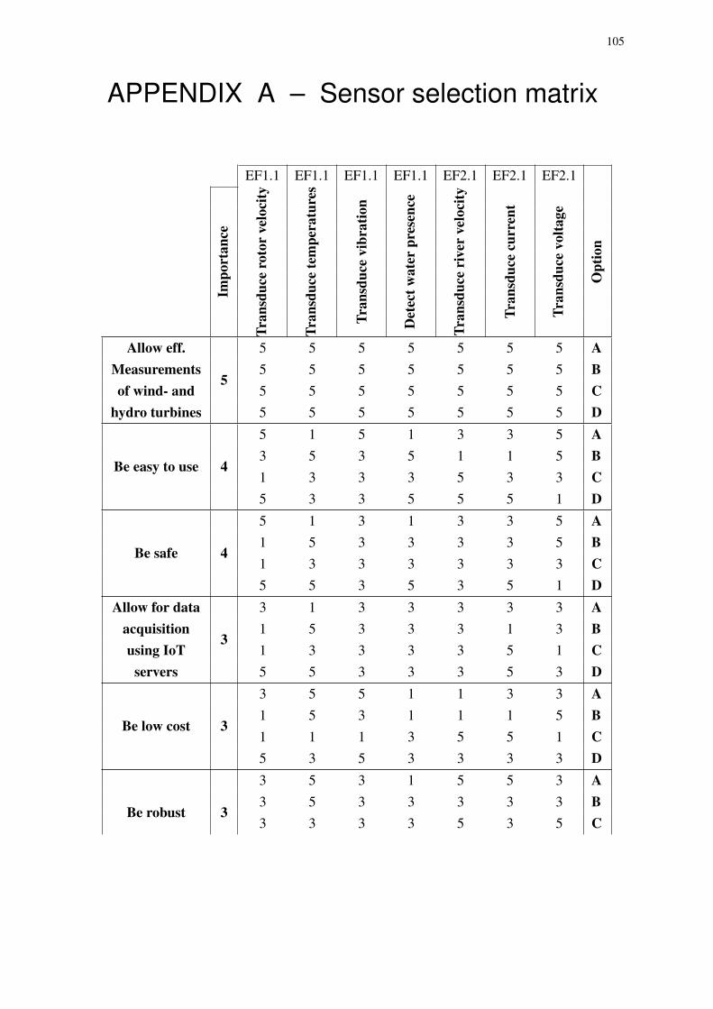
105
APPENDIX A – Sensor selection matrix
EF1.1 EF1.1 EF1.1 EF1.1 EF2.1 EF2.1 EF2.1
Impo
rtan
ce
T ran
sduc
ero
tor
velo
city
Tran
sduc
ete
mpe
ratu
res
T ran
sduc
evi
brat
ion
Det
ectw
ater
pres
ence
Tran
sduc
eri
ver
velo
city
Tran
sduc
ecu
rren
t
T ran
sduc
evo
ltage
Opt
ion
Allow eff.Measurementsof wind- and
hydro turbines
5
5 5 5 5 5 5 5 A5 5 5 5 5 5 5 B5 5 5 5 5 5 5 C5 5 5 5 5 5 5 D
Be easy to use 4
5 1 5 1 3 3 5 A3 5 3 5 1 1 5 B1 3 3 3 5 3 3 C5 3 3 5 5 5 1 D
Be safe 4
5 1 3 1 3 3 5 A1 5 3 3 3 3 5 B1 3 3 3 3 3 3 C5 5 3 5 3 5 1 D
Allow for dataacquisitionusing IoT
servers
3
3 1 3 3 3 3 3 A1 5 3 3 3 1 3 B1 3 3 3 3 5 1 C5 5 3 3 3 5 3 D
Be low cost 3
3 5 5 1 1 3 3 A1 5 3 1 1 1 5 B1 1 1 3 5 5 1 C5 3 5 3 3 3 3 D
Be robust 3
3 5 3 1 5 5 3 A3 5 3 3 3 3 3 B3 3 3 3 5 3 5 C
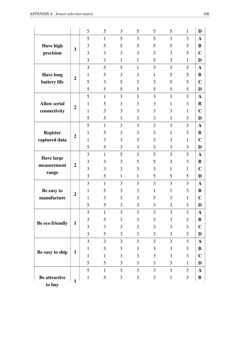
APPENDIX A. Sensor selection matrix 106
5 5 3 5 5 5 1 D
Have highprecision
3
5 1 5 3 5 3 3 A3 5 5 5 5 5 3 B3 3 3 3 3 3 5 C3 3 1 1 5 3 1 D
Have longbattery life
2
3 5 5 1 3 3 3 A1 5 3 3 1 5 5 B5 3 5 3 3 5 5 C5 5 5 5 5 5 5 D
Allow serialconnectivity
2
5 1 3 3 3 3 3 A1 5 3 3 3 1 3 B1 3 3 3 3 3 1 C5 5 3 3 3 3 3 D
Registercaptured data
2
5 1 3 3 3 3 3 A1 5 3 3 3 1 3 B1 3 3 3 3 3 1 C5 5 3 3 3 3 3 D
Have largemeasurement
range2
3 1 5 3 5 3 5 A3 3 3 5 5 3 3 B3 3 3 3 3 1 1 C3 5 1 1 5 5 5 D
Be easy tomanufacture
2
3 1 3 3 3 3 3 A1 5 3 3 1 1 3 B1 3 3 3 5 3 1 C5 5 3 3 3 3 3 D
Be eco friendly 1
3 1 3 3 3 3 3 A3 5 3 3 3 3 3 B3 3 3 3 3 3 3 C3 5 3 3 3 3 3 D
Be easy to ship 1
3 3 3 3 3 3 3 A1 5 3 3 3 3 3 B1 1 3 3 3 3 3 C5 5 3 3 3 3 1 D
Be attractiveto buy
1
5 1 3 3 3 3 3 A1 5 3 3 3 1 3 B

APPENDIX A. Sensor selection matrix 107
1 3 3 3 3 3 1 C5 5 3 3 3 3 1 D
Be easy todispose
1
3 1 3 3 3 3 3 A3 5 3 3 3 3 3 B3 5 3 3 3 3 3 C3 5 3 3 3 3 3 D
159 93 155 95 137 133 147 A87 191 133 139 115 103 153 B87 121 125 127 151 139 113 C
Sum of "optionscore" times
"importance"181 175 127 143 155 163 103 D
Table 13 – Selection matrix for sensors
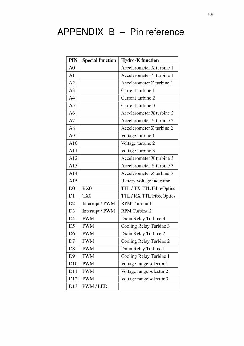
108
APPENDIX B – Pin reference
PIN Special function Hydro-K functionA0 Accelerometer X turbine 1
A1 Accelerometer Y turbine 1
A2 Accelerometer Z turbine 1
A3 Current turbine 1
A4 Current turbine 2
A5 Current turbine 3
A6 Accelerometer X turbine 2
A7 Accelerometer Y turbine 2
A8 Accelerometer Z turbine 2
A9 Voltage turbine 1
A10 Voltage turbine 2
A11 Voltage turbine 3
A12 Accelerometer X turbine 3
A13 Accelerometer Y turbine 3
A14 Accelerometer Z turbine 3
A15 Battery voltage indicator
D0 RX0 TTL / TX TTL FibreOptics
D1 TX0 TTL / RX TTL FibreOptics
D2 Interrupt / PWM RPM Turbine 1
D3 Interrupt / PWM RPM Turbine 2
D4 PWM Drain Relay Turbine 3
D5 PWM Cooling Relay Turbine 3
D6 PWM Drain Relay Turbine 2
D7 PWM Cooling Relay Turbine 2
D8 PWM Drain Relay Turbine 1
D9 PWM Cooling Relay Turbine 1
D10 PWM Voltage range selector 1
D11 PWM Voltage range selector 2
D12 PWM Voltage range selector 3
D13 PWM / LED
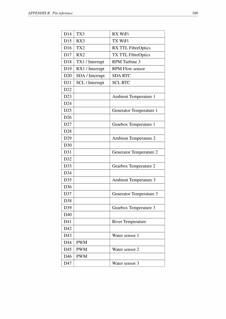
APPENDIX B. Pin reference 109
D14 TX3 RX WiFi
D15 RX3 TX WiFi
D16 TX2 RX TTL FibreOptics
D17 RX2 TX TTL FibreOptics
D18 TX1 / Interrupt RPM Turbine 3
D19 RX1 / Interrupt RPM Flow sensor
D20 SDA / Interrupt SDA RTC
D21 SCL / Interrupt SCL RTC
D22
D23 Ambient Temperature 1
D24
D25 Generator Temperature 1
D26
D27 Gearbox Temperature 1
D28
D29 Ambient Temperature 2
D30
D31 Generator Temperature 2
D32
D33 Gearbox Temperature 2
D34
D35 Ambient Temperature 3
D36
D37 Generator Temperature 3
D38
D39 Gearbox Temperature 3
D40
D41 River Temperature
D42
D43 Water sensor 1
D44 PWM
D45 PWM Water sensor 2
D46 PWM
D47 Water sensor 3

APPENDIX B. Pin reference 110
D48
D49
D50 MISO MISO SD Card
D51 MOSI MOSI SD Card
D52 SCK SCK SD Card
D53 CS CS SD Card
Table 14 – Pin reference
B.1 Instrumentation platform schematic
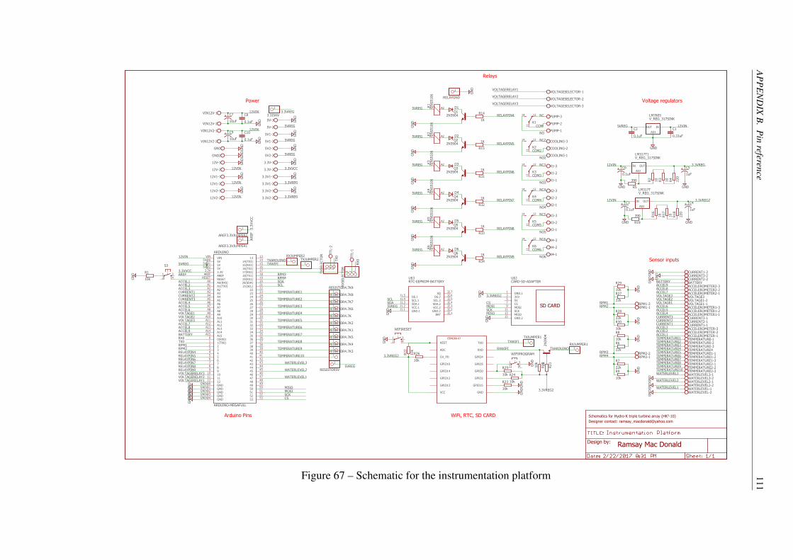
AP
PE
ND
IXB
.P
inreference
111
ARDUINO-MEGAFULL
GN
D
GN
DG
ND
GN
D
GN
DG
ND GN
D
GN
D
GN
DG
ND
GN
DG
ND
GN
D
ZN
S5106
2N3904
1K
GN
D
ZN
S5106
2N39041K
GN
D
10
V_REG_317SINK
1uF
10
220
390
10k
1k
10k
CARD-SD-ADAPTERRTC-EEPROM-BATTERY
10k
10k
10k
10k
22k
22k
10k
10k
GN
D
GN
D
ZN
S5106
2N39041K
GN
D
ZN
S5106
2N39041K
GN
D
ZN
S5106
2N39041K
GN
D
ZN
S5106
2N39041K
GN
DG
ND
GN
D
GN
D
GN
DG
ND
V_REG_317SINK
GND
GN
DG
ND
GN
DG
ND
GN
D
0.33uF0.1uF
0.1uF
GN
D
GN
D
10kGN
D
10
V_REG_317SINK
1uF
10
220
390
0.1uF
GND GND
GN
D
GND GND
GN
D
GN
DG
ND
GN
D
22k
22k
10k
10k
GN
DG
ND
GN
D
GN
D
10uF 0.1uF
10uF 0.1uF
ARDUINO
5V5V@0
RESETRESET
5V5V@1
A0(RX0)A0
A1(TX0)A1
A2A2
A3A3
A4A4
A5A5
A6A6
A7A7
A8A8
A9A9
A10A10
A11A11
A12A12
A13A13
A14A14
A15A15
1(TX0)1
22
33
44
55
66
77
88
99
1010
GNDGND@4
16(TX2)16
17(RX2)17
18(TX1)18
2222
2323
2424
2525
2626
2727
2828
2929
3030
3131
3232
3333
3434
3535
3636
3737
3838
4040
3939
4141
4242
4343
4444
4545
4646
4747
4848
1111
1212
1313
15(RX3)15
14(TX3)14
GNDGND@0
GNDGND@1
GNDGND@2
GNDGND@3
5353
5252
5151
5050
4949
5V5V@2
3.3V3.3V
AREFAREF
21(SCL)21
20(SDA)20
19(RX1)19
VINVIN
0(RX0)0
AREF3.3VJUMPER2
1
AREF3.3VJUMPER1
1
12V-1
12V-2
5V-1
5V-2
3.3V-1
3.3V-2
WATERLEVEL-1WATERLEVEL-2
VOLTAGE1-1VOLTAGE1-2
CURRENT1-1
CURRENT1-2
CURRENT2-1
CURRENT2-2
CURRENT3-1
CURRENT3-2
ACCELEROMETER-1ACCELEROMETER-2ACCELEROMETER-3
TEMPERATURE-1TEMPERATURE-2TEMPERATURE-3
K1
A2A1
K1
1214
11
D1
Q1 R14
K2
A2A1
K2
1214
11
D2
Q2
R15
PUMP-1
PUMP-2
PUMP-3
COOLING-1
COOLING-2
COOLING-3
GND
GND2
R16
ADJ
IN OUT
LM317T
C4
2N
3904
R17
R18
R19
R20
R21
R22
GND.11
3V33
5V5
CS7
MOSI9
SCK11
MISO13
GND.215
U$2
GND.1J1.1
VCC.1J1.2
SDA.1J1.3
SCL.1J1.4
DS.1J1.5
BATJ2.1
GND.2J2.2
VCC.2J2.3
SDA.2J2.4
SCL.2J2.5
DS.2J2.6
SQJ2.7
U$3
REST
ADC
CH_PD
GPIO16
GPIO14
GPIO12
GPIO13
VCC GND
GPIO15
GPIO2
GPIO0
GPIO5
GPIO4
RXD
TXD
R23
R24
R25
R26
ACCELEROMETER1-1ACCELEROMETER1-2ACCELEROMETER1-3
ACCELEROMETER2-1ACCELEROMETER2-2ACCELEROMETER2-3
TTL-1
TTL-2
RXSELECTO
R1 2 3TXSELECTO
R1 2 3
R27
R28
R29
R30
RPM1-1RPM1-2
K3
A2A1
K3
1214
11
D3
Q3
R31
K4
A2A1
K4
1214
11
D4
Q4
R32
K5
A2A1 K5
1214
11
D5
Q5
R33
K6
A2A1K6
1214
11D6
Q6
R34
VOLTAGESELECTOR-1
VOLTAGESELECTOR-2
VOLTAGESELECTOR-3
WATERLEVEL2-1WATERLEVEL2-2
WATERLEVEL3-1WATERLEVEL3-2
TEMPERATURE1-1TEMPERATURE1-2TEMPERATURE1-3TEMPERATURE2-1TEMPERATURE2-2TEMPERATURE2-3
TEMPERATURE4
VOLTAGE3
BATTERY
X1-1
X1-2
X1-3
X2-1
X2-2
X2-3
X3-1
X3-2
X3-3
X4-1
X4-2
X4-3
VIN12V-1
VIN12V-2
RXJUMPER11
TXJUMPER21
TXJUMPER11
RXJUMPER21
RELAYGND
1
12V1-1
12V1-2
12V2-1
12V2-2
ADJ
INOUT
LM7805
5V1-1
5V1-2
5V2-1
5V2-2
3.3V1-1
3.3V1-2
3.3V2-1
3.3V2-2
VIN12V2-1
VIN12V2-2
C1C2
C3
WIFIPROGRAM
1 342
WIFIRESET
1 342
RESISTOR4.7K1
RESISTOR4.7K11
RESISTOR4.7K21
RESISTOR4.7K31
RESISTOR4.7K41
RESISTOR4.7K51
RESISTOR4.7K61
RESISTOR4.7K71
RESISTOR4.7K81
RESISTOR4.7K91
RESISTOR5V
1
S3
1 342
R1
R2
ADJ
IN OUT
LM317T1
C5
R3
R4
R5
C6
3.3ISHV
1
R6
R7
R8
R9
RPM2-1RPM2-2
C7 C8
C9 C10
5VREG
5VREG
5VREG
5VREG
5VREG
5VREG
5VREG
5VREG
5VREG
5VREG
5VREG
5VREG
5VREG
3.3VVCC
3.3
VVCC
3.3VVCC
AREF
AREF
12VIN12VIN
12VIN
12VIN
12VIN
12VIN
12VIN
12VIN
12VIN
3.3VREG
3.3VREG
3.3VREG
3.3VREG
3.3VREG2
3.3VREG2
3.3VREG2
3.3VREG2
RXWIFI
TXWIFI
TXWIFI
SDA
SDA
SCL
SCL
TXARDUINO
TXARDUINO
WATERLEVEL3
WATERLEVEL3WATERLEVEL2
WATERLEVEL2WATERLEVEL1
WATERLEVEL1
VOLTAGERELAY3
VOLTAGERELAY3
VOLTAGERELAY1
VOLTAGERELAY1
VOLTAGERELAY2
VOLTAGERELAY2
RPM1
RPM1
RPM2
RPM2
RPM3
RPM3
RPM4
RPM4RELAYPIN4
RELAYPIN4
RELAYPIN5
RELAYPIN5
RELAYPIN6
RELAYPIN6
RELAYPIN7
RELAYPIN7
RELAYPIN8
RELAYPIN8
RELAYPIN9
RELAYPIN9
CS
CS
MOSI
MOSIMISO
MISO
SCK
SCK
TEMPERATURE1
TEMPERATURE1
TEMPERATURE2
TEMPERATURE2
TEMPERATURE3
TEMPERATURE3
TEMPERATURE4
TEMPERATURE4
TEMPERATURE5
TEMPERATURE5
TEMPERATURE6
TEMPERATURE6
TEMPERATURE7
TEMPERATURE7
TEMPERATURE8
TEMPERATURE8
TEMPERATURE9
TEMPERATURE9
TEMPERATURE10
TEMPERATURE10
RX0
RX0TX0
TX0
ACCEL1
ACCEL1
ACCEL8
ACCEL8
BATTERY
BATTERY
ACCEL2
ACCEL2
ACCEL3
ACCEL3
CURRENT1
CURRENT1
CURRENT2
CURRENT2
CURRENT3
CURRENT3
ACCEL4
ACCEL4
ACCEL5ACCEL5 ACCEL6ACCEL6
VOLTAGE1
VOLTAGE1
VOLTAGE2
VOLTAGE2
VOLTAGE3
VOLTAGE3
ACCEL7
ACCEL7
ACCEL9
ACCEL9
NO
COM
NC
NC2
COM2
NO2
NC3
NC4
NC5
NC6
NO3
NO4
NO5
NO6
COM3
COM4
COM5
COM6
SD CARD
ESP8266-07
Schematics for Hydro-K triple turbine array (HK3-10)Designer contact: [email protected]
Design by:
Power
Arduino Pins WiFi, RTC, SD CARD
Sensor inputs
Relays
Voltage regulators
Ramsay Mac Donald
Figure 67 – Schematic for the instrumentation platform
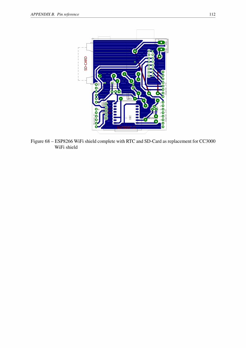
APPENDIX B. Pin reference 112
10
10
220
390
10k
1k10k
2N3904
C1
C2
R1
R2
R3
R4
R5
R6R7
RXARDUINO
TXARDUINO
U$1
D7
X1
D8
D2
D3
E$1
E$2
1
2
ESP8266-12
SD-CARD
RTC
Figure 68 – ESP8266 WiFi shield complete with RTC and SD-Card as replacement for CC3000WiFi shield
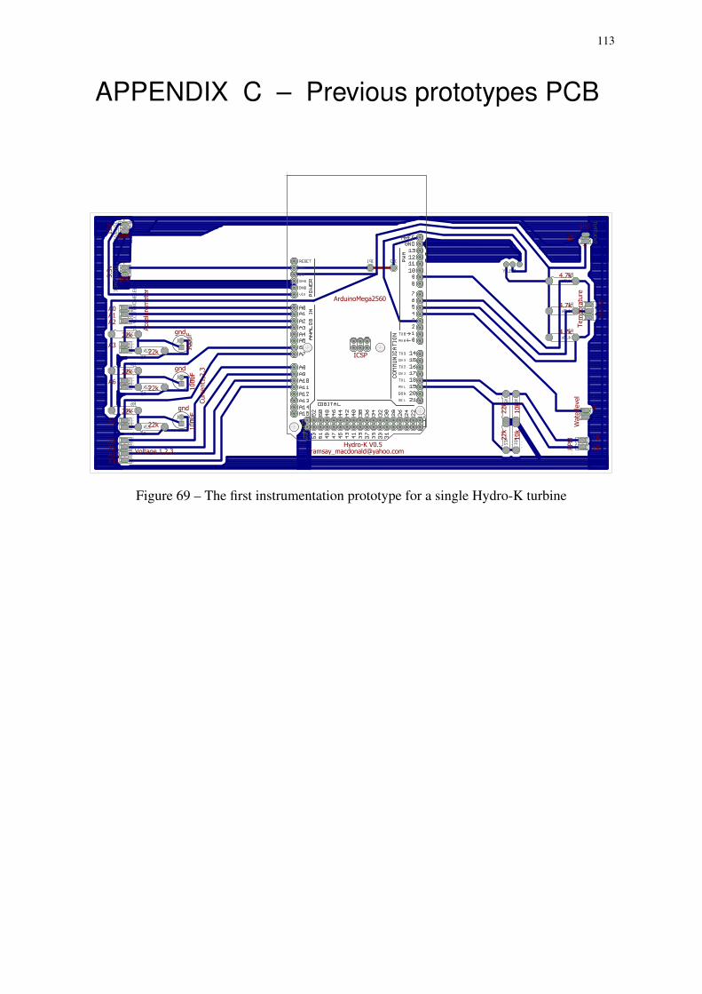
113
APPENDIX C – Previous prototypes PCB
4.7k
4.7k
4.7k
22k
22k
22k
22k
22k
22k
22k
22k
10k
10k
12VINPUT
ACCELEROMETER
C1
C2
C3
C
U
R
R
E
N
T
1
C
U
R
R
E
N
T
2
C
U
R
R
E
N
T
3
R1
R2
R3
R4
R5
R6
R7
R8
R9
R
P
M
1
E
2
V
O
L
T
A
G
E
I
N
1
V
O
L
T
A
G
E
I
N
2
RELAY
R
1
0
R
1
1
R
1
2
R
1
3
JP1
1
1
1
1
1
1
1
1
1
1
1
1
gnd
22k
22k
22k
ArduinoMega2560
ICSP
100uF
100uf
3.3VOUTPUT
5VOUTPUT
T
E
M
P
E
R
A
T
U
R
E
1
W
A
T
E
R
L
E
V
E
L
3.3
v
gnd
gnd
gnd
4.7k
4.7k
4.7k22k
22k
22k
22k
22k
10k
10k
100uf
100uF
100uf
100uF
965
4
18
19RPM
Wate
rlevel
Tem
pera
ture
5V1
2V
Curr
ent1
,2,3
A7
A6
A3
Voltage 1,2,3
A8A9A10A11
A0A1A2
Acc
ele
rom
ete
r
Hydro-K [email protected]
JP2+
gnd
gnd
+
+
Figure 69 – The first instrumentation prototype for a single Hydro-K turbine
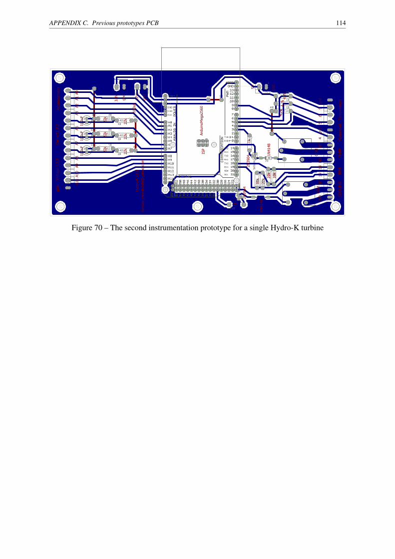
APPENDIX C. Previous prototypes PCB 114
100uf
100uf
100uf
4.7k
22k22k
22k22k
22k22k
22k
22k
10k
10k
ZNS5106
2N3904
1K
ZNS51062N3904
1K
C1
C2
C3
R1
R2
R4
R5
R6
R7
R8
R9
R
1
0
R
1
1
R
1
2
R
1
3
JP1 JP2
12V3.3V
W
A
T
E
R
L
E
V
E
L
V
O
L
T
A
G
E
1
V
O
L
T
A
G
E
2
C
U
R
R
E
N
T
1
C
U
R
R
E
N
T
2
C
U
R
R
E
N
T
3
R
P
M
A
C
C
E
L
E
R
O
M
E
T
E
R
JP3
K1
D1Q
1
R
1
4
K2
D2
Q
2
M
P
O
L
I
N
G
JP4G
N
D
JP5
JP6
JP7
JP8
JP9
JP10
JP11
G
N
D
2
1
2
3
1
2
3
1
2
3
1
2
3
1
2
1
2
1212
1
2
1
2
1
2
1
2
1
2
1
2
1
2
22k
22k
22k
22k
22k
22k
10k
100uF
100uF
Ard
uin
oM
ega2560
ISP
1k
22k
10k
1N
4148
22k
100uF
Hydro
-K V
1.0
ram
say_m
acd
onald
@yahoo.c
om
4.7k
4.7k
R35V
12
gnd
+
RPM
Wate
rlevel
Tem
pera
ture
Curr
ent1
,2,3
Voltage 1
,2,3
Acc
ele
rom
ete
r 5V
gnd
4.7
k4.7
k
PU
MP
CO
OLIN
G
44..77
kk
1N
4148
T
E
M
P
E
R
A
T
U
9RE
R15
NOPU
NOCO
418
19
A7
A6
A3
A11
A10
A9
A8
A2
A1
A0
gnd
CO
MCO
M
1k
2N
3904
2N
3904
gndgnd
100uF
65
3.3
V
NC
NC
12V
gnd
Figure 70 – The second instrumentation prototype for a single Hydro-K turbine

115
APPENDIX D – Latest prototype PCB
!
!
!
""
""
Battery Voltage
"""""#""
""
""
$
$
%
%
&
&
'
'
'
%
&
%
&
%
&
%
&
$
$
$
$
$
$
(
!
!
)
)
)
)
%
%
*
)
)
)
++
)
)
))
)
)
)
)
!
%
!
%
!
%
!
%
*
*
*
)
*
*
ArduinoMega2560
Hydro-K [email protected]
Real Time Clock
SD Card
Figure 71 – The first instrumentation prototype for all three Hydro-K turbines
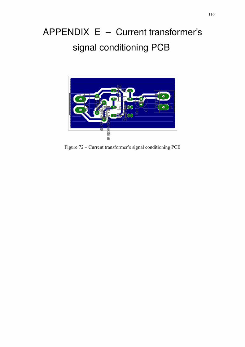
116
APPENDIX E – Current transformer’s
signal conditioning PCB
12
12
C1
D1
D2
D3
D4
BURDENRESISTOR
INPUT
OUTPUT
BURDENRESISTOR1
10uF
100ohm
100ohm
Figure 72 – Current transformer’s signal conditioning PCB

117
APPENDIX F – Voltage divider PCB
!
"#
$
%
&
&
'%
$%#
%%(
%%(
%%(
(((
(
(
(
%(
)*#
#+,-.
Figure 73 – Voltage sensor with selectable resolution

118
APPENDIX G – Amplifier PCB
1k
100
100
100
1k
100
1k1k
0.22uF0.22uF
100
100
100
100
10k
1k
1k
2.2k
10k
22k
1M100k
10nF
0.1uF
10uF
10k
R1
GAIN
R3
R4
R5
R7
V
VOUT
VIN
R2
R8
C1C2
R9
R10
R11
R12
R13
R14
R15
R16
R17
R18
R19
R20
C3
C4
C5
R21
1
21
2
1
2
R6
IC2
100
LM324N
GND
GND
12V
SIG
IN+
IN-
Figure 74 – PCB of designed water flow sensor

119
APPENDIX H – Arduino Code
1 //Instrumentation platform sketch
2 //Written by Ramsay Mac Donald
4 //WARNING!!! DO NOT CONNECT THE ARDUINO TO ANY COMPUTER WHEN HIGH VOLTAGES ARE BEING MEASURED
5 #include <ESP8266.h>
6 #include <Modbus.h>
7 #include <ModbusIP_ESP8266AT.h>
8 //-----------------------------------------------------------------------------Wifi Pre Program
9 ESP8266 wifi(Serial3, 115200);
10 const String wifiNetwork = "WhyPhy"; //Enter the WiFi network name here
11 const String password = "P@ssw0rd"; //Enter the WiFi network password here
12 ModbusIP mb;
13 #define NUMBER_OF_REGISTERS 31 //How many parameters will you send using WiFi?
14 int IREGS[NUMBER_OF_REGISTERS];
15 int data2send[NUMBER_OF_REGISTERS];
16 //-------------------------------------------------------------------------------SD Pre Program
17 #include <SD.h>
18 #include <SPI.h>
19 const int chipSelect = 53; //Independent of which pin you select, always keep 53 as an OUTPUT
20 #define NUMBER_OF_SDVARIABLES 31 //How many parameters will you save on the SD Card?
21 char fileName[16];
22 //------------------------------------------------------------------------------RTC Pre Program
23 #include <Wire.h>
24 #include "RTClib.h"
25 RTC_DS1307 RTC;
26 //----------------------------------------------------------------------Temperature Pre Program
27 #include <OneWire.h>
28 #define NUMBER_OF_BUSSES 10 //How many temperatures busses will you use?
29 #define NUMBER_OF_COOLING_RELAYS 3 //How many cooling pumps will you control?
30 #define COOLING_START_TEMP 55 //Cooling pump on threshold
31 #define COOLING_STOP_TEMP 50 //Cooling pump off threshold
32 // AT1, GT1, MT1, AT2, GT2, MT2, AT3, GT3, MT3, riverTemp
33 const int busList[NUMBER_OF_BUSSES] = 23, 25, 27, 29, 31, 33, 35, 37, 39, 41; //bus pins
34 OneWire *ds[NUMBER_OF_BUSSES];
35 float celsius[NUMBER_OF_BUSSES];
36 byte busMatrix[NUMBER_OF_BUSSES][12];
37 byte addrMatrix[NUMBER_OF_BUSSES][8];
38 const int coolingRelayPins[NUMBER_OF_COOLING_RELAYS] = 9, 7, 5; //Set cooling relay pins
39 boolean tempTrigger [NUMBER_OF_COOLING_RELAYS] = false, false, false;
40 unsigned long tempCompareTime[NUMBER_OF_COOLING_RELAYS] = 0, 0, 0;
41 boolean coolingRelayState[NUMBER_OF_COOLING_RELAYS] = 0, 0, 0;
42 //-------------------------TEMPERATURE CLOCK---------------------------------------------------
43 unsigned long zero = 0;
44 unsigned long PTR = 0; //PreviousTemperatureRead
45 const unsigned long ONE = 1000; //OneSecondInterval
46 boolean ReadOK = true; //Check if temperature has been read
47 //------------------------------------------------------------------------------RPM Pre Program
48 #define NUMBER_OF_INTERRUPTS 4 //Declare number of pins for interrupt (RPM sensors)
49 float RPM[NUMBER_OF_INTERRUPTS];
50 // turbine1, turbine2, turbine3, riverVelocity
51 const int RPMpin[NUMBER_OF_INTERRUPTS] = 3, 2, 18, 19;//Declare which pins to attach interrupt
52 unsigned long pulse[NUMBER_OF_INTERRUPTS];
53 const int pulsesPerRot[NUMBER_OF_INTERRUPTS] = 10, 10, 60, 60;//Declare how many pulses per rotation
54 boolean inter = false;
55 //--------------------------------------------------------------------Accelerometer Pre Program
56 #define NUMBER_OF_ACCEL 3 //Declare number of accelerometers
57 #define NUMBER_OF_AXES 3 //Declare number of axes
58 #define SAMPLE_SIZE 64 //Declare how many samples to take the average from

APPENDIX H. Arduino Code 120
59 // accelerometerAmplitude[0][0] = X-turbine 1, accelerometerAmplitude[0][1] = Y-turbine 1,
accelerometerAmplitude[0][2] = Z-turbine 1
60 // accelerometerAmplitude[1][0] = X-turbine 2, accelerometerAmplitude[1][1] = Y-turbine 2,
accelerometerAmplitude[1][2] = Z-turbine 2
61 // accelerometerAmplitude[2][0] = X-turbine 3, accelerometerAmplitude[2][1] = Y-turbine 3,
accelerometerAmplitude[2][2] = Z-turbine 3
62 const int accelerometerPins[NUMBER_OF_ACCEL][NUMBER_OF_AXES] =
63 A0, A1, A2,
64 A6, A7, A8,
65 A12, A13, A14
66 ;
67 int accelerometerAmplitude[NUMBER_OF_ACCEL][NUMBER_OF_AXES];
68 //--------------------------------------------------------------------------Voltage Pre Program
69 #define NUMBER_OF_VOLTAGE_SENSORS 3 //Declare number of voltage sensors
70 #define AX_axbVOLTAGEACTIVE 1.131 //Voltage sensor calibration relay on
71 #define B_axbVOLTAGEACTIVE 0 //Voltage sensor calibration relay on
72 #define AX_axbVOLTAGE 0.5711 //Voltage sensor calibration relay off
73 #define B_axbVOLTAGE 0 //Voltage sensor calibration relay off
74 // voltageVal[0] = turbine 1, voltageVal[1] = turbine 2, voltageVal[2] = turbine 3
75 const int voltageSensors[NUMBER_OF_VOLTAGE_SENSORS] = A9, A10, A11; //Voltage sensor pins
76 // resolutionRelayPins[0] = turbine 1, resolutionRelayPins[1] = turbine 2, resolutionRelayPins[2] =
turbine 3
77 const int resolutionRelayPins[NUMBER_OF_VOLTAGE_SENSORS] = 10, 11, 12; //Voltage relay pins
78 float voltageVal[NUMBER_OF_VOLTAGE_SENSORS];
79 unsigned long compareTime[NUMBER_OF_VOLTAGE_SENSORS] = 0, 0, 0;
80 boolean relayInTransition[NUMBER_OF_VOLTAGE_SENSORS] = false, false, false;
81 //--------------------------------------------------------------------------Current Pre Program
82 #define NUMBER_OF_CURRENT_SENSORS 3 //Declare number of current sensors
83 #define AX_axbCURRENT 0.0316 //Current sensor calibration
84 #define B_axbCURRENT 3.2206 //Current sensor calibration
85 // currentVal[0] = turbine 1, currentVal[1] = turbine 2, currentVal[2] = turbine 3
86 const int currentSensors[NUMBER_OF_CURRENT_SENSORS] = A3, A4, A5; //Declare current pins
87 float currentVal[NUMBER_OF_CURRENT_SENSORS];
88 //---------------------------------------------------------------------Water Sensor Pre Program
89 #define NUMBER_OF_DIGITAL_SWITCHES 3 //Declare number of water sensors
90 // turbine1, turbine2, turbine3
91 const int switchPins[NUMBER_OF_DIGITAL_SWITCHES] = 43, 45, 47; //Water sensor pins
92 // turbine1, turbine2, turbine3
93 const int drainPins[NUMBER_OF_DIGITAL_SWITCHES] = 8, 6, 4; //Drainage pump pins
94 boolean waterPresent[NUMBER_OF_DIGITAL_SWITCHES] = false, false, false;
95 boolean lastPresenceState[NUMBER_OF_DIGITAL_SWITCHES] = false, false, false;
96 unsigned long presenceCompareTime[NUMBER_OF_DIGITAL_SWITCHES] = 0, 0, 0;
97 //----------------------------------------------------------------------------Relay Pre Program
98 #define NUMBER_OF_RELAYS 9 //Declare number of relays
99 //cool1, drain1, cool2, drain2, cool3, drain3, Vsel1, Vsel2, Vsel3
100 const int relayPins[NUMBER_OF_RELAYS] = 9, 8, 7, 6, 5, 4, 10, 11, 12; //Relay pins
101 //--------------------------------------------------------------------------Program Pre Program
102 #define NUMBER_OF_TURBINES 3 //Declare number of turbines
103 long ts;
104 unsigned long CTime = 0; //Reference of current time
105 //---------------------------------------------------------------------------------------------
106 //---------------------------------------------------------------------------------------------
107 //-------------------------------------------------------------------------------WiFi Functions
108 //------------------------CREATE REGISTERS FUNCTION--------------------------------------------
109 void addRegisters(int IREG[])
110
111 for (int r = 0; r < NUMBER_OF_REGISTERS; r++)
112 IREG[r] = r + 1;
113 mb.addIreg(IREG[r]);
114
115
116 //---------------------------------------------------------------------------------SD Functions
117 //------------------------END SD LINE FUNCTION-------------------------------------------------
118 void endLineSD(int chipselect, char filen[16])
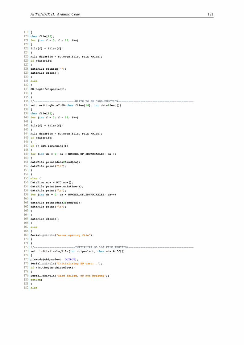
APPENDIX H. Arduino Code 121
119
120 char file[16];
121 for (int f = 0; f < 16; f++)
122
123 file[f] = filen[f];
124
125 File dataFile = SD.open(file, FILE_WRITE);
126 if (dataFile)
127
128 dataFile.println("");
129 dataFile.close();
130
131 else
132
133 SD.begin(chipselect);
134
135
136 //------------------------WRITE TO SD CARD FUNCTION--------------------------------------------
137 void writingDataToSD(char filen[16], int data2Send[])
138
139 char file[16];
140 for (int f = 0; f < 16; f++)
141
142 file[f] = filen[f];
143
144 File dataFile = SD.open(file, FILE_WRITE);
145 if (dataFile)
146
147 if (! RTC.isrunning())
148
149 for (int da = 0; da < NUMBER_OF_SDVARIABLES; da++)
150
151 dataFile.print(data2Send[da]);
152 dataFile.print("\t");
153
154
155 else
156 DateTime now = RTC.now();
157 dataFile.print(now.unixtime());
158 dataFile.print("\t");
159 for (int da = 0; da < NUMBER_OF_SDVARIABLES; da++)
160
161 dataFile.print(data2Send[da]);
162 dataFile.print("\t");
163
164
165 dataFile.close();
166
167 else
168
169 Serial.println("error opening file");
170
171
172 //------------------------INITIALIZE SD LOG FILE FUNCTION--------------------------------------
173 void initializeLogFile(int chipselect, char charBuff[])
174
175 pinMode(chipselect, OUTPUT);
176 Serial.println("Initializing SD card...");
177 if (!SD.begin(chipselect))
178
179 Serial.println("Card failed, or not present");
180 return;
181
182 else

APPENDIX H. Arduino Code 122
183
184 DateTime now = RTC.now();
185 if (! RTC.isrunning())
186
187 Serial.println("RTC not running");
188 for (int a = 0; a < 99; a++)
189
190 if (a < 9)
191
192 int b = a + 1;
193 String number = String(b);
194 String file = "log0" + number + ".txt";
195 file.toCharArray(charBuff, 16);
196 if (SD.exists(charBuff))
197
198 Serial.print(charBuff); Serial.println(" present");
199
200 else
201
202 Serial.print("Writing to "); Serial.println(charBuff);
203 File dataFile = SD.open(charBuff, FILE_WRITE);
204 if (dataFile)
205
206 dataFile.println("No RTC");
207 dataFile.close();
208
209 else
210 Serial.println("error opening file");
211
212 break;
213
214
215 else
216
217 int b = a + 1;
218 String number = String(b);
219 String file = "log" + number + ".txt";
220 file.toCharArray(charBuff, 16);
221 if (SD.exists(charBuff))
222
223 Serial.print(charBuff); Serial.println(" present");
224
225 else
226
227 Serial.print("Writing to "); Serial.println(charBuff);
228 File dataFile = SD.open(charBuff, FILE_WRITE);
229 if (dataFile)
230
231 dataFile.println("No RTC");
232 dataFile.close();
233
234 else
235
236 Serial.println("error opening file");
237
238 break;
239
240
241
242
243 else
244 int ye = now.year();
245 int mo = now.month();
246 int da = now.day();
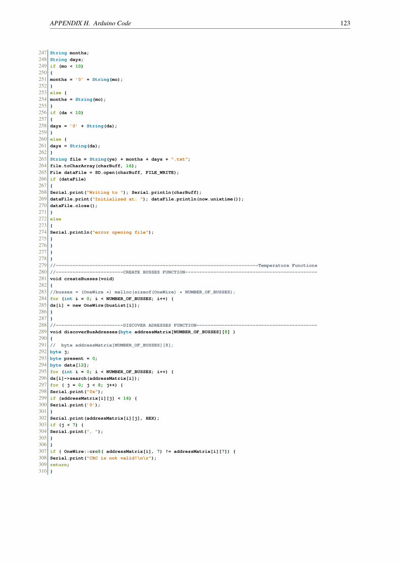
APPENDIX H. Arduino Code 123
247 String months;
248 String days;
249 if (mo < 10)
250
251 months = ’0’ + String(mo);
252
253 else
254 months = String(mo);
255
256 if (da < 10)
257
258 days = ’0’ + String(da);
259
260 else
261 days = String(da);
262
263 String file = String(ye) + months + days + ".txt";
264 file.toCharArray(charBuff, 16);
265 File dataFile = SD.open(charBuff, FILE_WRITE);
266 if (dataFile)
267
268 Serial.print("Writing to "); Serial.println(charBuff);
269 dataFile.print("Initialized at: "); dataFile.println(now.unixtime());
270 dataFile.close();
271
272 else
273
274 Serial.println("error opening file");
275
276
277
278
279 //------------------------------------------------------------------------Temperature Functions
280 //------------------------CREATE BUSSES FUNCTION-----------------------------------------------
281 void createBusses(void)
282
283 //busses = (OneWire *) malloc(sizeof(OneWire) * NUMBER_OF_BUSSES);
284 for (int i = 0; i < NUMBER_OF_BUSSES; i++)
285 ds[i] = new OneWire(busList[i]);
286
287
288 //------------------------DISCOVER ADRESSES FUNCTION-------------------------------------------
289 void discoverBusAdresses(byte addressMatrix[NUMBER_OF_BUSSES][8] )
290
291 // byte addressMatrix[NUMBER_OF_BUSSES][8];
292 byte j;
293 byte present = 0;
294 byte data[12];
295 for (int i = 0; i < NUMBER_OF_BUSSES; i++)
296 ds[i]->search(addressMatrix[i]);
297 for ( j = 0; j < 8; j++)
298 Serial.print("0x");
299 if (addressMatrix[i][j] < 16)
300 Serial.print(’0’);
301
302 Serial.print(addressMatrix[i][j], HEX);
303 if (j < 7)
304 Serial.print(", ");
305
306
307 if ( OneWire::crc8( addressMatrix[i], 7) != addressMatrix[i][7])
308 Serial.print("CRC is not valid!\n\r");
309 return;
310
APPENDIX H. Arduino Code 124
311 Serial.println();
312 Serial.print("pin: ");
313 Serial.println(busList[i]);
314 ds[i]->reset_search();
315
316
317 //------------------------REQUEST TEMPERATURE FUNCTION-----------------------------------------
318 void requestTemperature(void)
319
320 for (int r = 0; r < NUMBER_OF_BUSSES; r++)
321 ds[r]->reset();
322 ds[r]->select(addrMatrix[r]);
323 ds[r]->write(0x44, 1);
324
325
326 //------------------------READ TEMPERATURE FUNCTION--------------------------------------------
327 void readTemp(float temp[NUMBER_OF_BUSSES])
328 for (int s = 0; s < NUMBER_OF_BUSSES; s++)
329
330 ds[s]->reset();
331 ds[s]->select(addrMatrix[s]);
332 ds[s]->write(0xBE);
333 for ( byte i = 0; i < 9; i++) // we need 9 bytes
334 busMatrix[s][i] = ds[s]->read();
335
336 int16_t raw = (busMatrix[s][1] << 8) | busMatrix[s][0]; // Convert to actual temperature
337 temp[s] = (float)raw / 16.0; // because the result is a 16 bit signed integer, it should
338
339
340 //------------------------AUTOMATICALLY CHANGE COOLING RELAY STATE FUNCTION--------------------
341 void controlCoolingRelayState(const int coolingrelaypins[], const float temperatures[], unsigned long
tempcomparetime[], boolean trigger[], boolean coolingrelaystate[])
342
343 unsigned long referenceTime[NUMBER_OF_COOLING_RELAYS];
344 float maxTemp[NUMBER_OF_COOLING_RELAYS] = 0, 0, 0;
345 float tempmatrix[NUMBER_OF_COOLING_RELAYS][NUMBER_OF_COOLING_RELAYS];
346 for (int X = 0; X < NUMBER_OF_COOLING_RELAYS; X++)
347
348 if (X == 0)
349
350 for (int Z = 0; Z < 3; Z++)
351
352 tempmatrix[X][Z] = temperatures[Z];
353
354
355 if (X == 1)
356
357 for (int Z = 3; Z < 6; Z++)
358
359 tempmatrix[X][Z - 3] = temperatures[Z];
360
361
362 if (X == 2)
363
364 for (int Z = 6; Z < 9; Z++)
365
366 tempmatrix[X][Z - 6] = temperatures[Z];
367
368
369
370 for (int Y = 0; Y < 3; Y++)
371
372 maxTemp[Y] = max(tempmatrix[Y][0], tempmatrix[Y][1]);
373 maxTemp[Y] = max(maxTemp[Y], tempmatrix[Y][2]);
APPENDIX H. Arduino Code 125
374
375 boolean button[NUMBER_OF_COOLING_RELAYS] false, false, false;
376 for (int sst = 0; sst < NUMBER_OF_COOLING_RELAYS; sst++)
377
378 referenceTime[sst] = millis();
379 if (maxTemp[sst] > COOLING_START_TEMP) button[sst] = true;
380 else if (maxTemp[sst] < COOLING_STOP_TEMP) button[sst] = false;
381 else button[sst] = trigger[sst];
382 if (button[sst] != trigger[sst]) tempcomparetime[sst] = referenceTime[sst];
383 if (tempcomparetime[sst] + 500UL < referenceTime[sst])
384
385 if (button[sst] != coolingrelaystate[sst])
386 coolingrelaystate[sst] = ! coolingrelaystate[sst];
387 digitalWrite(coolingrelaypins[sst], coolingrelaystate[sst]);
388
389
390 trigger[sst] = button[sst];
391
392
393 //--------------------------------------------------------------------------------RPM Functions
394 //------------------------attachInterrupts FUNCTION--------------------------------------------
395 void attachInterrupts(int interruptPins[])
396
397 attachInterrupt(digitalPinToInterrupt(interruptPins[0]), rotCounter, FALLING);
398 if (NUMBER_OF_INTERRUPTS < 2) return;
399 attachInterrupt(digitalPinToInterrupt(interruptPins[1]), rotCounter1, FALLING);
400 if (NUMBER_OF_INTERRUPTS < 3) return;
401 attachInterrupt(digitalPinToInterrupt(interruptPins[2]), rotCounter2, FALLING);
402 if (NUMBER_OF_INTERRUPTS < 4) return;
403 attachInterrupt(digitalPinToInterrupt(interruptPins[3]), rotCounter3, FALLING);
404 if (NUMBER_OF_INTERRUPTS < 5) return;
405 attachInterrupt(digitalPinToInterrupt(interruptPins[4]), rotCounter4, FALLING);
406 if (NUMBER_OF_INTERRUPTS < 6) return;
407 attachInterrupt(digitalPinToInterrupt(interruptPins[5]), rotCounter5, FALLING);
408
409 //------------------------detachInterrupts FUNCTION--------------------------------------------
410 void detachInterrupts(int interruptPins[])
411
412 for (int p; p < NUMBER_OF_INTERRUPTS; p++)
413
414 detachInterrupt(digitalPinToInterrupt(interruptPins[p]));
415
416
417 //------------------------checkZeroRPM FUNCTION------------------------------------------------
418 void checkZeroRPM(float RPMval[], unsigned long lastPulse[])
419
420 for (int c; c < NUMBER_OF_INTERRUPTS; c++)
421
422 if (micros() - lastPulse[c] >= 5000000 || RPMval[c] >= 2000)
423 RPMval[c] = 0;
424
425
426
427 //------------------------RPM FUNCTIONS--------------------------------------------------------
428 // Here there are 6 rotCounter functions because there’s a maximum
429 // of 6 interrupt pins on Arduino Mega.
430 // There will be no rollover problem as long as "unsigned long" is used
431 // and a pulse was measured within 71.5 minutes. If not, only the first
432 // measurement will be incorrect.
433 //------------------------rotCounter1 FUNCTION-------------------------------------------------
434 void rotCounter()
435
436 volatile unsigned long cPulse = micros();
437 volatile const int n = 0;

APPENDIX H. Arduino Code 126
438 RPM[n] = ((float) 60.0 / (float) pulsesPerRot[n]) * (float) ((float) 1000000.00 / (cPulse - pulse[n]));
439 pulse[n] = cPulse;
440
441 //------------------------rotCounter2 FUNCTION-------------------------------------------------
442 void rotCounter1()
443
444 volatile unsigned long cPulse = micros();
445 volatile const int n = 1;
446 RPM[n] = ((float) 60.0 / (float) pulsesPerRot[n]) * (float) ((float) 1000000.00 / (cPulse - pulse[n]));
447 pulse[n] = cPulse;
448
449 //------------------------rotCounter3 FUNCTION-------------------------------------------------
450 void rotCounter2()
451
452 volatile unsigned long cPulse = micros();
453 volatile const int n = 2;
454 RPM[n] = ((float) 60.0 / (float) pulsesPerRot[n]) * (float) ((float) 1000000.00 / (cPulse - pulse[n]));
455 pulse[n] = cPulse;
456
457 //------------------------rotCounter4 FUNCTION-------------------------------------------------
458 void rotCounter3()
459
460 volatile unsigned long cPulse = micros();
461 volatile const int n = 3;
462 RPM[n] = ((float) 60.0 / (float) pulsesPerRot[n]) * (float) ((float) 1000000.00 / (cPulse - pulse[n]));
463 pulse[n] = cPulse;
464
465 //------------------------rotCounter5 FUNCTION-------------------------------------------------
466 void rotCounter4()
467
468 volatile unsigned long cPulse = micros();
469 volatile const int n = 4;
470 RPM[n] = ((float) 60.0 / (float) pulsesPerRot[n]) * (float) ((float) 1000000.00 / (cPulse - pulse[n]));
471 pulse[n] = cPulse;
472
473 //------------------------rotCounter6 FUNCTION-------------------------------------------------
474 void rotCounter5()
475
476 volatile unsigned long cPulse = micros();
477 volatile const int n = 5;
478 RPM[n] = ((float) 60.0 / (float) pulsesPerRot[n]) * (float) ((float) 1000000.00 / (cPulse - pulse[n]));
479 pulse[n] = cPulse;
480
481 //----------------------------------------------------------------------Accelerometer Functions
482 //------------------------INITIALIZE ACCELEROMETERS FUNCTION-----------------------------------
483 void initializeAccelerometers(const int accelerometers[NUMBER_OF_ACCEL][NUMBER_OF_AXES])
484
485 for (int rea = 0; rea < NUMBER_OF_ACCEL; rea++)
486
487 for (int rea2 = 0; rea2 < NUMBER_OF_ACCEL; rea2++)
488
489 pinMode(accelerometers[rea][rea2], INPUT);
490
491
492
493 //------------------------MEASURE AMPLITUDES FUNCTION------------------------------------------
494 void readAmplitudes(const int accelerometers[NUMBER_OF_ACCEL][NUMBER_OF_AXES], int accelerometeramplitude[
NUMBER_OF_ACCEL][NUMBER_OF_AXES])
495
496 int tempMatrix[NUMBER_OF_ACCEL][NUMBER_OF_AXES];
497 int minMatrix[NUMBER_OF_ACCEL][NUMBER_OF_AXES];
498 int maxMatrix[NUMBER_OF_ACCEL][NUMBER_OF_AXES];
499 for (int q = 0; q < SAMPLE_SIZE; q++)
500
APPENDIX H. Arduino Code 127
501 for (int x = 0; x < NUMBER_OF_ACCEL; x++)
502
503 for (int y = 0; y < NUMBER_OF_AXES; y++)
504
505 tempMatrix[x][y] = analogRead(accelerometers[x][y]);
506 if (q == 0)
507
508 minMatrix[x][y] = tempMatrix[x][y];
509 maxMatrix[x][y] = tempMatrix[x][y];
510
511 if (tempMatrix[x][y] < minMatrix[x][y]) minMatrix[x][y] = tempMatrix[x][y];
512 if (tempMatrix[x][y] > maxMatrix[x][y]) maxMatrix[x][y] = tempMatrix[x][y];
513
514
515
516 for (int s = 0; s < NUMBER_OF_ACCEL; s++)
517
518 for (int t = 0; t < NUMBER_OF_AXES; t++)
519
520 accelerometeramplitude[s][t] = maxMatrix[s][t] - minMatrix[s][t];
521
522
523
524 //----------------------------------------------------------------------------Voltage Functions
525 //------------------------INITIALIZE VOLTAGE SENSORS FUNCTION----------------------------------
526 void initializeVoltageSensors(const int voltagesensors[])
527
528 for (int rev = 0; rev < NUMBER_OF_VOLTAGE_SENSORS; rev++)
529
530 pinMode(voltagesensors[rev], INPUT);
531
532
533 //------------------------INITIALIZE SWITCH RELAYS FUNCTION------------------------------------
534 void initializeResolutionRelays(const int relaypins[])
535
536 for (int rer = 0; rer < NUMBER_OF_VOLTAGE_SENSORS; rer++)
537
538 pinMode(relaypins[rer], OUTPUT);
539 digitalWrite(relaypins[rer], LOW);
540
541
542 //------------------------CHECK IF RELAY IS ACTIVE FUNCTION------------------------------------
543 bool resolutionRelayActive(int relaypin)
544
545 bool relayState = digitalRead(relaypin);
546 if (relayState == true) return true;
547 else return false;
548
549 //------------------------AUTOMATICALLY CHANGE VOLT RELAY STATE FUNCTION-----------------------
550 void selectVoltRelayState(const int relaypins[], const int vSensorPins[], unsigned long comparetime[],
boolean trigger[])
551
552 unsigned long referenceTime[NUMBER_OF_VOLTAGE_SENSORS];
553 int inputV[NUMBER_OF_VOLTAGE_SENSORS];
554 boolean button[NUMBER_OF_VOLTAGE_SENSORS] false, false, false;
555 for (int ssr = 0; ssr < NUMBER_OF_VOLTAGE_SENSORS; ssr++)
556
557 referenceTime[ssr] = millis();
558 inputV[ssr] = analogRead(vSensorPins[ssr]);
559 if (inputV[ssr] > 900) button[ssr] = true;
560 else if (inputV[ssr] < 450) button[ssr] = false;
561 else button[ssr] = trigger[ssr];
562 if (button[ssr] != trigger[ssr]) comparetime[ssr] = referenceTime[ssr];
563 if (comparetime[ssr] + 500UL < referenceTime[ssr])
APPENDIX H. Arduino Code 128
564
565 if (button[ssr] != resolutionRelayActive(relaypins[ssr])) digitalWrite(relaypins[ssr], button[ssr]);
566
567 trigger[ssr] = button[ssr];
568
569
570 //------------------------READ VOLTAGE FUNCTION------------------------------------------------
571 void readVolt(float voltageval[], int voltagesensors[])
572
573 for (int coun = 0; coun < NUMBER_OF_VOLTAGE_SENSORS; coun++)
574
575 if (resolutionRelayActive)
576
577 voltageval[coun] = (analogRead(voltagesensors[coun]) * AX_axbVOLTAGEACTIVE) + B_axbVOLTAGEACTIVE;
578
579 else
580
581 voltageval[coun] = (analogRead(voltagesensors[coun]) * AX_axbVOLTAGE) + B_axbVOLTAGE;
582
583
584
585 //----------------------------------------------------------------------------Current Functions
586 //------------------------INITIALIZE CURRENT SENSORS FUNCTION----------------------------------
587 void initializeCurrentSensors(const int currentsensors[])
588
589 for (int rec = 0; rec < NUMBER_OF_CURRENT_SENSORS; rec++)
590
591 pinMode(currentsensors[rec], INPUT);
592
593
594 //------------------------READ CURRENT FUNCTION------------------------------------------------
595 void readAmp(float currentval[], int currentsensors[])
596
597 for (int cou = 0; cou < NUMBER_OF_CURRENT_SENSORS; cou++)
598
599 currentval[cou] = (analogRead(currentsensors[cou]) * AX_axbCURRENT) + B_axbCURRENT;
600
601
602 //-----------------------------------------------------------------------Water Sensor Functions
603 //------------------------INITIALIZE SWITCHES FUNCTION-----------------------------------------
604 void initializeSwitches(int switchpins[])
605
606 for (int swi = 0; swi < NUMBER_OF_DIGITAL_SWITCHES; swi++)
607
608 pinMode(switchpins[swi], INPUT);
609 digitalWrite(switchpins[swi], HIGH);
610
611
612 //------------------------READ WATER PRESENCE FUNCTION-----------------------------------------
613 void readWaterPresence(const int switchpins[], unsigned long presencecomparetime[], bool trigger[],
boolean switchstate[], const int drainpins[])
614
615 unsigned long referenceTime[NUMBER_OF_DIGITAL_SWITCHES];
616 int IO[NUMBER_OF_DIGITAL_SWITCHES];
617 for (int rwr = 0; rwr < NUMBER_OF_DIGITAL_SWITCHES; rwr++)
618
619 referenceTime[rwr] = millis();
620 IO[rwr] = digitalRead(switchpins[rwr]);
621 if (IO[rwr] != trigger[rwr]) presencecomparetime[rwr] = referenceTime[rwr];
622 if (presencecomparetime[rwr] + 500UL < referenceTime[rwr])
623
624 if (IO[rwr] == switchstate[rwr])
625
626 switchstate[rwr] = !switchstate[rwr];
APPENDIX H. Arduino Code 129
627 digitalWrite(drainpins[rwr], switchstate[rwr]);
628
629
630 trigger[rwr] = IO[rwr];
631
632
633 //------------------------INITIALIZE DRAIN RELAYS FUNCTION-------------------------------------
634 void initializeDrainRelays(const int drainpins[])
635
636 for (int rer = 0; rer < NUMBER_OF_DIGITAL_SWITCHES; rer++)
637
638 pinMode(drainpins[rer], OUTPUT);
639 digitalWrite(drainpins[rer], LOW);
640
641
642 //-----------------------------------------------------------------------------Relays Functions
643 //------------------------INITIALIZE RELAYS FUNCTION-------------------------------------------
644 void initializeRelays(int relaypins[])
645
646 for (int re = 0; re < NUMBER_OF_RELAYS; re++)
647
648 pinMode(relaypins[re], OUTPUT);
649 digitalWrite(relaypins[re], LOW);
650
651
652 //---------------------------------------------------------------------End of Program Functions
653 //---------------------------------------------------------------------------------------------
654 //---------------------------------------------------------------------------------------------
655 //---------------------------------------------------------------------------------------------
656 //-------------------------PROGRAM SETUP-------------------------------------------------------
657 void setup()
658 //--------------------------------------------------------------------------------------------
659 //---------------------------------------------------------------------------------Serial Setup
660 Serial.begin(115200); //Initialize serial communication and set baudrate
661 //------------------------------------------------------------------------------------RTC Setup
662 //initialize RTC
663 Wire.begin();
664 RTC.begin();
665 if (! RTC.isrunning())
666 Serial.println("RTC is NOT running!");
667 //The following line sets the RTC to the date & time this sketch was compiled
668 RTC.adjust(DateTime(__DATE__, __TIME__));
669
670 RTC.adjust(DateTime(__DATE__, __TIME__));
671 //-----------------------------------------------------------------------------------WiFi Setup
672 //Initialize WiFi
673 mb.config(wifi, wifiNetwork, password);
674 //Add SENSOR_IREG register - Use addIreg() for analog Inputs
675 addRegisters(IREGS);
676 //-------------------------------------------------------------------------------------SD Setup
677 //Make sure that the default chip select pin is set to
678 //output, even if you don’t use it. For Arduino Mega:
679 //pinMode(53, OUTPUT);
680 //Initialize SD card and create or select the log file
681 initializeLogFile(chipSelect, fileName);
682 //----------------------------------------------------------------------------Temperature Setup
683 //Initialize busses
684 createBusses();
685 //Discover and allocate addresses connected to the busses
686 discoverBusAdresses(addrMatrix);
687 initializeRelays(coolingRelayPins);
688 //------------------------------------------------------------------------------------RPM Setup
689 //Initialize interrupt pins
690 if (inter == false)
APPENDIX H. Arduino Code 130
691 attachInterrupts(RPMpin);
692 inter = true;
693
694 //--------------------------------------------------------------------------Accelerometer Setup
695 initializeAccelerometers(accelerometerPins);
696 //--------------------------------------------------------------------------------Voltage Setup
697 initializeResolutionRelays(resolutionRelayPins);
698 initializeVoltageSensors(voltageSensors);
699 //--------------------------------------------------------------------------------Current Setup
700 initializeCurrentSensors(currentSensors);
701 //---------------------------------------------------------------------------Water Sensor Setup
702 initializeSwitches(switchPins);
703 initializeDrainRelays(drainPins);
704 //----------------------------------------------------------------------------------Relay Setup
705 //initializeRelays(relayPins);
706 //--------------------------------------------------------------------------------Program Setup
707 zero = millis() + 3000UL; //Reference (only start the program when current time is zero time)
708 PTR = zero; //Previous time read
709 ts = millis(); //Refernce time for data saving and sending
710 //------------------------MAIN CODE-----------------------------------------------------------
711 void loop()
712 //-------------------------------------------------------------------------------------------
713 //---------------------------------------------------------------------------------------------
714 //---------------------------------------------------------------------------------------------
715 //---------------------------------------------------------------------------------------------
716 //---------------------------------------------------------------------------------------------
717 //---------------------------------------------------------------------------------------------
718 //----------------------------------------------------------------------------Synchronize Clock
719 while (millis() < zero) //set clock "zero" (to avoid functions running too soon after setup)
720 CTime = millis();//use CTime to sync several functions (if no sync is needed just use millis())
721 //------------------------------------------------------------------RPM Sensor Main Code PART 1
722 //Re-attachInterrupts after modbus transmission
723 attachInterrupts(RPMpin);
724 //------------------------------------------------------------------------Temperature Main Code
725 if (ReadOK) //If previous temperature reading has finished
726 requestTemperature(); //Send new tempereature reading request
727 ReadOK = false;
728
729 if (PTR + ONE <= CTime) //If one second has passed since data request
730 //celsius[] = AT1, GT1, MT1, AT2, GT2, MT2, AT3, GT3, MT3, riverTemp
731 readTemp(celsius); //Read requested temperature data
732 for (int nt = 0; nt < NUMBER_OF_BUSSES; nt++)
733 //data2send[0] - data2send[9] for Temperature
734 data2send[nt] = celsius[nt];
735
736 ReadOK = true;
737 PTR += ONE;
738
739 //Check if cooling needs to be applied. If so, apply cooling
740 //IMPORTANT!! The following automatically switches relay to keep turbine at a safe temperature
741 controlCoolingRelayState(coolingRelayPins, celsius, tempCompareTime, tempTrigger, coolingRelayState);
742 //---------------------------------------------------------------------Voltage Sensor Main Code
743 //Check if the voltage sensor relay has to be activated, and act accordingly
744 //IMPORTANT!! The following automatically switches relay to keep pin voltage lower than 5V
745 selectVoltRelayState(resolutionRelayPins, voltageSensors, compareTime, relayInTransition);
746 // voltageVal[0] = turbine 1, voltageVal[1] = turbine 2, voltageVal[2] = turbine 3
747 readVolt(voltageVal, voltageSensors); //Read voltage data
748 for (int nv = 0; nv < NUMBER_OF_VOLTAGE_SENSORS; nv++)
749 // data2send[10] - data2send[12] for Voltage
750 data2send[nv + NUMBER_OF_BUSSES] = voltageVal[nv];
751
752 //-----------------------------------------------------------------------Water Sensor Main Code
753 //Check if water needs to be pumped out, and act accordingly
754 //IMPORTANT!! The following automatically switches relay to pump water out of the turbine

APPENDIX H. Arduino Code 131
755 readWaterPresence(switchPins, presenceCompareTime, lastPresenceState, waterPresent, drainPins);
756 // waterPresent[0] = turbine 1, waterPresent[1] = turbine 2, waterPresent[2] = turbine 3
757 for (int nw = 0; nw < NUMBER_OF_DIGITAL_SWITCHES; nw++)
758 //data2send[13] - data2send[15] for Water Presence
759 data2send[nw + NUMBER_OF_BUSSES + NUMBER_OF_VOLTAGE_SENSORS] = waterPresent[nw];
760
761 //----------------------------------------------------------------------Accelerometer Main Code
762 // accelerometerAmplitude[0][0] = X-turbine 1, accelerometerAmplitude[0][1] = Y-turbine 1,
accelerometerAmplitude[0][2] = Z-turbine 1
763 // accelerometerAmplitude[1][0] = X-turbine 2, accelerometerAmplitude[1][1] = Y-turbine 2,
accelerometerAmplitude[1][2] = Z-turbine 2
764 // accelerometerAmplitude[2][0] = X-turbine 3, accelerometerAmplitude[2][1] = Y-turbine 3,
accelerometerAmplitude[2][2] = Z-turbine 3
765 readAmplitudes(accelerometerPins, accelerometerAmplitude); //Read vibration amplitudes data
766 for (int na = 0; na < NUMBER_OF_ACCEL; na++)
767 //data2send[16] - data2send[24] for Accelerometers
768 for (int nax = 0; nax < NUMBER_OF_AXES; nax++)
769
770 data2send[(nax + NUMBER_OF_BUSSES + NUMBER_OF_VOLTAGE_SENSORS + NUMBER_OF_DIGITAL_SWITCHES) + (na * 3)] =
accelerometerAmplitude[na][nax];
771
772
773 //---------------------------------------------------------------------Current Sensor Main Code
774 // currentVal[0] = turbine 1, currentVal[1] = turbine 2, currentVal[2] = turbine 3
775 readAmp(currentVal, currentSensors); //Read current data
776 for (int nc = 0; nc < NUMBER_OF_CURRENT_SENSORS; nc++)
777 //data2send[25] - data2send[27] for Current
778 data2send[nc + NUMBER_OF_BUSSES + NUMBER_OF_VOLTAGE_SENSORS + NUMBER_OF_DIGITAL_SWITCHES + (
NUMBER_OF_ACCEL * NUMBER_OF_AXES)] = currentVal[nc];
779
780 //------------------------------------------------------------------RPM Sensor Main Code PART 2
781 // RPM[0] = turbine 1, RPM[1] = turbine 2, RPM[2] = turbine 3
782 checkZeroRPM(RPM, pulse); //Check if RPM is zero, if so change RPM to zero
783 for (int nr = 0; nr < NUMBER_OF_CURRENT_SENSORS; nr++)
784 //data2send[28] - data2send[30] for RPM
785 data2send[nr + NUMBER_OF_BUSSES + NUMBER_OF_VOLTAGE_SENSORS + NUMBER_OF_DIGITAL_SWITCHES + (
NUMBER_OF_ACCEL * NUMBER_OF_AXES) + NUMBER_OF_CURRENT_SENSORS] = RPM[nr];
786
787 detachInterrupts(RPMpin); //DetachInterrupts for better modbus transmission
788 inter = false;
789 //----------------------------------------------------------------------------Debugging Purpose
790 // //
791 //WARNING!! DO NOT CONNECT THE ARDUINO TO ANY COMPUTER WHEN HIGH VOLTAGES ARE BEING MEASURED//
792 /*793 for (int n = 0; n < NUMBER_OF_REGISTERS; n++)
794
795 data2send[n] = n + 1;
796 Serial.print(data2send[n]); //Serial print data that will be saved and sent
797 Serial.print("\t");
798
799 //Serial.println();
800 for (int j = 0; j < NUMBER_OF_VOLTAGE_SENSORS; j++)
801
802 Serial.print(voltageVal[j]); //Serial print voltage data
803 Serial.print("\t");
804 Serial.print(resolutionRelayActive(resolutionRelayPins[j]));//Serial print relay is on or off
805 Serial.print("\t");
806
807 //Serial.println();
808 for (int tint = 0; tint < NUMBER_OF_BUSSES; tint++)
809
810 Serial.print(celsius[tint]); //Serial print temperature data
811 Serial.print(" C ");
812

APPENDIX H. Arduino Code 132
813 //Serial.println();
814 for (int i = 0; i < NUMBER_OF_DIGITAL_SWITCHES; i++)
815
816 Serial.print(waterPresent[i]); //Serial print water presence
817 Serial.print("\t");
818
819 //Serial.println();
820 for (int l = 0; l < NUMBER_OF_ACCEL; l++)
821
822 for (int m = 0; m < NUMBER_OF_ACCEL; m++)
823
824 Serial.print(accelerometerAmplitude[l][m]); //Serial print vibration data
825 Serial.print("\t");
826
827 Serial.println();
828
829 //Serial.println();
830 for (int jee = 0; jee < NUMBER_OF_CURRENT_SENSORS; jee++)
831
832 Serial.print(currentVal[jee]); //Serial print current data
833 Serial.print("\t");
834
835 //Serial.println();
836 for (int c; c < NUMBER_OF_INTERRUPTS; c++)
837
838 Serial.print(RPM[c]); //Serial print RPM data
839 Serial.print("\t");
840
841 Serial.println();
842 */
843 //---------------------------------------------------Modbus, SD, Serial (Data Output) Main Code
844 //Initialize modbus
845 mb.task();
846 //Print each three hundred miliseconds
847 if (millis() > ts + 300)
848
849 writingDataToSD(fileName, data2send);
850 endLineSD(chipSelect, fileName);
851 // send data2send via modbus
852 for (int dn = 0; dn < NUMBER_OF_REGISTERS; dn++)
853
854 Serial.print(data2send[dn]);
855 Serial.print("\t");
856 mb.Ireg(IREGS[dn], data2send[dn]);
857
858 ts = millis();
859
860 //----------------------------------------------------------------------------Debugging Purpose
861 /*Serial.println(millis() - CTime);*/ //Serial print time spent on loop
862 //-------------------------END-----------------------------------------------------------------
863 //--------------------------------------------------------------------------------End of Sketch
The sketch file displayed above is available at:<https://mega.nz/#!aJhGEC5D!hmLKN-enZim1f8_C2-g4qqHUhVSgjJ-X3omA0N3A5C8>
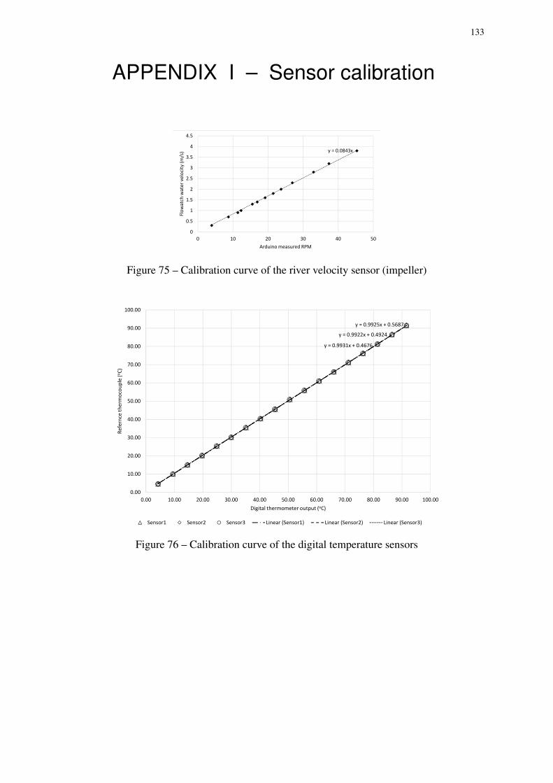
133
APPENDIX I – Sensor calibration
y = 0.0843x
0
0.5
1
1.5
2
2.5
3
3.5
4
4.5
0 10 20 30 40 50
Flo
wa
tch
wa
ter
velo
city
(m
/s)
Arduino measured RPM
Figure 75 – Calibration curve of the river velocity sensor (impeller)
y = 0.9931x + 0.4676
y = 0.9922x + 0.4924
y = 0.9925x + 0.5687
0.00
10.00
20.00
30.00
40.00
50.00
60.00
70.00
80.00
90.00
100.00
0.00 10.00 20.00 30.00 40.00 50.00 60.00 70.00 80.00 90.00 100.00
Re
fern
ce t
he
rmo
cou
ple
(oC
)
Digital thermometer output (oC)
Sensor1 Sensor2 Sensor3 Linear (Sensor1) Linear (Sensor2) Linear (Sensor3)
Figure 76 – Calibration curve of the digital temperature sensors
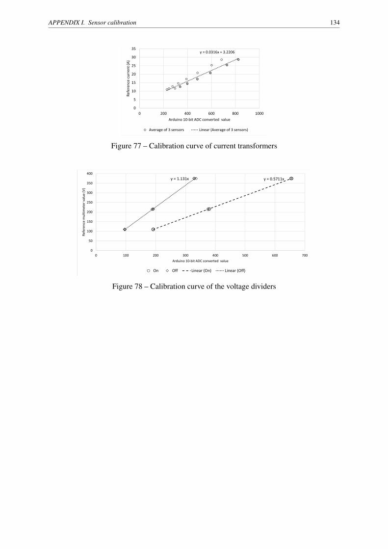
APPENDIX I. Sensor calibration 134
y = 0.0316x + 3.2206
0
5
10
15
20
25
30
35
0 200 400 600 800 1000
Re
fere
nce
cu
rre
nt
(A)
Arduino 10-bit ADC converted value
Average of 3 sensors Linear (Average of 3 sensors)
Figure 77 – Calibration curve of current transformers
y = 0.5711xy = 1.131x
0
50
100
150
200
250
300
350
400
0 100 200 300 400 500 600 700
Re
fere
nce
mu
ltim
ete
r va
lue
(V
)
Arduino 10-bit ADC converted value
On Off Linear (On) Linear (Off)
Figure 78 – Calibration curve of the voltage dividers