Instrumental Variables (IV)

Instrumental Variables (IV) is a method of estimation that is widely used

in many economic applications when correlation between the explanatory

variables and the error term is suspected

- for example, due to omitted variables, measurement error, or other sources

of simultaneity bias

1

Context

yi = x′iβ + ui for i = 1, ..., N

The basic idea is that if we can replace the actual realized values of xi

(which are correlated with ui) by predicted values of xi that are

- related to the actual xi

- but uncorrelated with ui

then we can obtain a consistent estimator of β

2

Predicted values are formed by projecting xi on a set of instrumental

variables or instruments, which are required to have two important prop-

erties:

- related to the explanatory variable(s) xi (‘informative’)

- uncorrelated with the errors ui (‘valid’)

The first property ensures that the predicted values are related to xi

The second property ensures that the predicted values are uncorrelated

with ui

3

The general problem in practice is finding instrumental variables that have

both these properties

But assuming for the moment that we have good instruments available, we

consider the method of Two Stage Least Squares (2SLS)

Note that in the context of multiple regression when some xi variables

are ‘endogenous’(i.e. correlated with ui) and other explanatory variables

are ‘exogenous’(i.e. uncorrelated with ui), the instruments are required to

have explanatory power for (each of) the endogenous xi variable(s) after

conditioning on all the remaining exogenous xi variable(s)

4

Two Stage Least Squares (2SLS)

We first consider a model with a single endogenous explanatory variable

(xi) and a single instrument (zi) - both assumed to have mean zero for

simplicity

yi = xiβ + ui for i = 1, ..., N E(ui) = 0, E(xiui) 6= 0

y = Xβ + u (all vectors are N × 1)

First stage regression (linear projection)

xi = ziπ + ri for i = 1, ..., N

X = Zπ + r (all vectors are N × 1)

5

We require

E(ziui) = 0

so that the instrumental variable zi is valid

We require

π 6= 0 (here↔ E(zixi) 6= 0)

so that the instrumental variable zi is informative

6

We estimate the first stage regression coeffi cient π using OLS

π = (Z ′Z)−1Z ′X

And form the predicted values of X = (x1, ..., xN)′

X = Zπ = Z(Z ′Z)−1Z ′X

Second stage regression

yi = xiβ + (ui + (xi − xi)β) for i = 1, ..., N

y = Xβ + (u + (X − X)β) (all vectors are N × 1)

The second component of the error term is a source of finite sample bias but

not inconsistency; also has to be noted when constructing standard errors7

We estimate the second stage regression coeffi cient β using OLS

β2SLS = (X ′X)−1X ′y

= [(Z(Z ′Z)−1Z ′X)′(Z(Z ′Z)−1Z ′X)]−1(Z(Z ′Z)−1Z ′X)′y

= [(X ′Z(Z ′Z)−1Z ′)(Z(Z ′Z)−1Z ′X)]−1(X ′Z(Z ′Z)−1Z ′)y

= [X ′Z(Z ′Z)−1Z ′Z(Z ′Z)−1Z ′X ]−1X ′Z(Z ′Z)−1Z ′y

= (X ′Z(Z ′Z)−1Z ′X)−1X ′Z(Z ′Z)−1Z ′y

using the symmetry of (Z ′Z)−1 s.t. [(Z ′Z)−1]′ = (Z ′Z)−1

8

The 2SLS estimator can also be written as

β2SLS = (X ′Z(Z ′Z)−1Z ′X)−1X ′Z(Z ′Z)−1Z ′y

= [(Z(Z ′Z)−1Z ′X)′X ]−1(Z(Z ′Z)−1Z ′X)′y

= (X ′X)−1X ′y

Notice that β2SLS = βOLS in the special case where zi = xi and hence

xi = xi

This is very intuitive - if we project xi on itself, we obtain perfect pre-

dictions and the second stage of 2SLS coincides with the standard OLS

regression9

The previous expressions for the 2SLS estimator remain valid when we have

several explanatory variables (in the row vector x′i) and several instrumental

variables (in the row vector z′i), in place of the scalars xi and zi [although, as

we will see, the requirements for β2SLS to be consistent become more subtle

in this case]

Only in the (just-identified) special case where we have the same

number of instruments as we have explanatory variables (i.e. where the row

vectors x′i and z′i have the same number of columns), we can also express the

2SLS estimator as

β2SLS = (Z ′X)−1Z ′y10

In the special case with one explanatory variable and one instrument, this

follows from X = Zπ with π being a scalar, using

β2SLS = (X ′X)−1X ′y = [(Zπ)′X ]−1(Zπ)′y

= [π(Z ′X)]−1π(Z ′y)

=1

π(Z ′X)−1π(Z ′y)

= (Z ′X)−1Z ′y

11

Proof of consistency

β2SLS = (X ′X)−1X ′y

= (X ′X)−1X ′(Xβ + u)

= (X ′X)−1X ′Xβ + (X ′X)−1X ′u

= β +

(X ′X

N

)−1(X ′u

N

)

Taking probability limits

p limN→∞

β2SLS = β + p limN→∞

(X ′X

N

)−1

p limN→∞

(X ′u

N

)

We assume the data on (yi, xi, zi) are independent over i = 1, ..., N

12

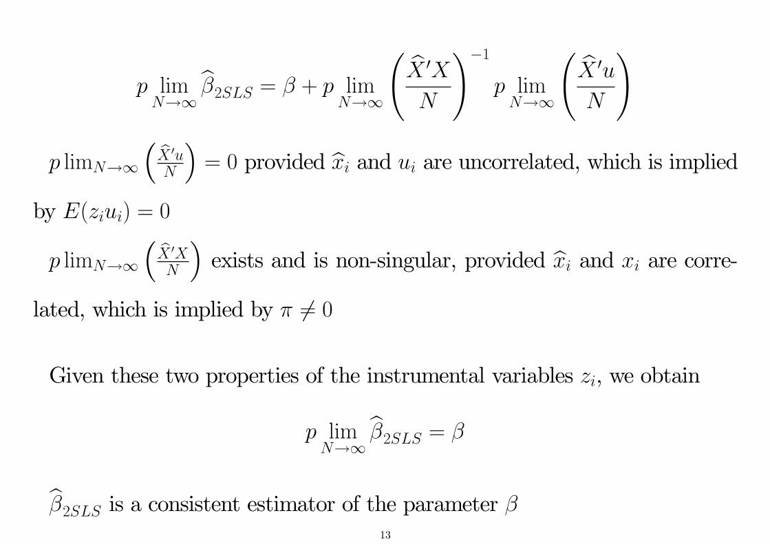
p limN→∞

β2SLS = β + p limN→∞

(X ′X

N

)−1

p limN→∞

(X ′u

N

)

p limN→∞

(X ′uN

)= 0 provided xi and ui are uncorrelated, which is implied

by E(ziui) = 0

p limN→∞

(X ′XN

)exists and is non-singular, provided xi and xi are corre-

lated, which is implied by π 6= 0

Given these two properties of the instrumental variables zi, we obtain

p limN→∞

β2SLS = β

β2SLS is a consistent estimator of the parameter β13

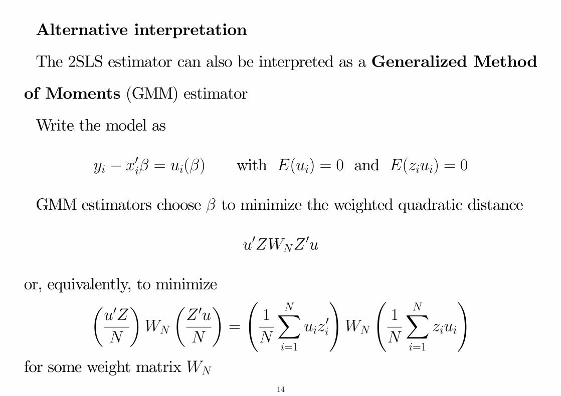
Alternative interpretation

The 2SLS estimator can also be interpreted as a Generalized Method

of Moments (GMM) estimator

Write the model as

yi − x′iβ = ui(β) with E(ui) = 0 and E(ziui) = 0

GMM estimators choose β to minimize the weighted quadratic distance

u′ZWNZ′u

or, equivalently, to minimize(u′Z

N

)WN

(Z ′u

N

)=

(1

N

N∑i=1

uiz′i

)WN

(1

N

N∑i=1

ziui

)for some weight matrix WN

14

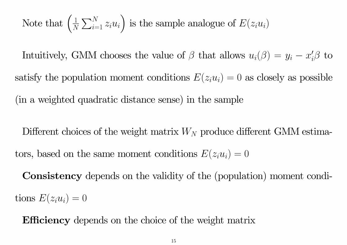
Note that(

1N

∑Ni=1 ziui

)is the sample analogue of E(ziui)

Intuitively, GMM chooses the value of β that allows ui(β) = yi − x′iβ to

satisfy the population moment conditions E(ziui) = 0 as closely as possible

(in a weighted quadratic distance sense) in the sample

Different choices of the weight matrixWN produce different GMM estima-

tors, based on the same moment conditions E(ziui) = 0

Consistency depends on the validity of the (population) moment condi-

tions E(ziui) = 0

Effi ciency depends on the choice of the weight matrix

15

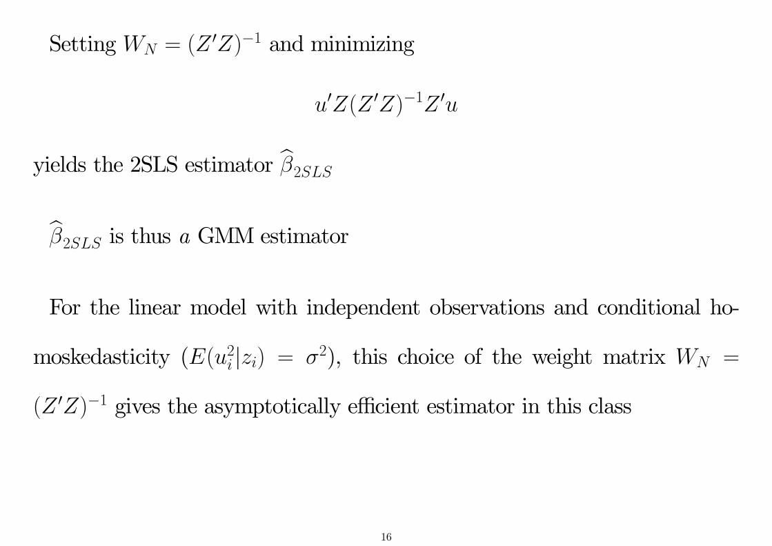
Setting WN = (Z ′Z)−1 and minimizing

u′Z(Z ′Z)−1Z ′u

yields the 2SLS estimator β2SLS

β2SLS is thus a GMM estimator

For the linear model with independent observations and conditional ho-

moskedasticity (E(u2i |zi) = σ2), this choice of the weight matrix WN =

(Z ′Z)−1 gives the asymptotically effi cient estimator in this class

16

For ‘just-identified’models, with the same number of instrumental vari-

ables in zi as explanatory variables in xi, the choice of the weight matrix is

irrelevant, since the 2SLS estimator makes ui(β) = yi−x′iβ and zi orthogonal

in the sample

This effi cient GMM interpretation provides a more general rationale for

2SLS in the ‘over-identified’case, where the number of instruments exceeds

the number of explanatory variables, and the choice of the weight matrix

matters for asymptotic effi ciency

Aside - OLS is a just-identifiedGMMestimator, obtained by setting zi = xi

17

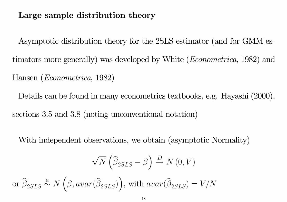
Large sample distribution theory

Asymptotic distribution theory for the 2SLS estimator (and for GMM es-

timators more generally) was developed by White (Econometrica, 1982) and

Hansen (Econometrica, 1982)

Details can be found in many econometrics textbooks, e.g. Hayashi (2000),

sections 3.5 and 3.8 (noting unconventional notation)

With independent observations, we obtain (asymptotic Normality)

√N(β2SLS − β

)D→ N (0, V )

or β2SLSa∼ N

(β, avar(β2SLS)

), with avar(β2SLS) = V/N

18

In large samples, hypothesis tests about the true value of some or all of

the elements of the parameter vector β can thus be conducted using fa-

miliar standard Normal or chi-squared test statistics, provided a consistent

estimator of avar(β2SLS) is available

Under the conditional homoskedasticity assumption that E(u2i |zi) = σ2,

the asymptotic variance of β2SLS is given by

avar(β2SLS) = σ2(X ′Z(Z ′Z)−1Z ′X)−1

= σ2(X ′X

)−1

19

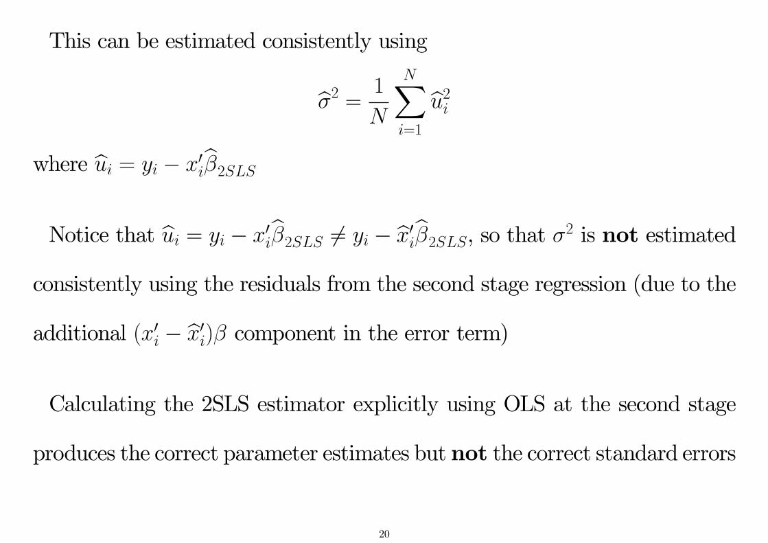
This can be estimated consistently using

σ2 =1

N

N∑i=1

u2i

where ui = yi − x′iβ2SLS

Notice that ui = yi − x′iβ2SLS 6= yi − x′iβ2SLS, so that σ2 is not estimated

consistently using the residuals from the second stage regression (due to the

additional (x′i − x′i)β component in the error term)

Calculating the 2SLS estimator explicitly using OLS at the second stage

produces the correct parameter estimates but not the correct standard errors

20

Many software programs are now available that produce 2SLS estimates

with the correct standard errors

The basic command that does this in Stata is ivregress

The syntax for specifying which explanatory variables are treated as en-

dogenous, which explanatory variables are treated as exogenous, and which

additional variables are used as instruments, is described in the Handout on

IV Estimation Using Stata

21

Importantly, we can also obtainheteroskedasticity-consistent (White/

Huber) standard errors for the 2SLS estimator (and for GMM estimators

more generally)

This is important because although themodel with conditional homoskedas-

ticity provides a useful theoretical benchmark, models with conditionally

heteroskedastic errors are very common in applied research

- we do not expect shocks hitting rich and poor households to be draws

from the same distribution

- we do not expect shocks hitting large and small firms to be draws from

the same distribution

22

Provided large samples are available - so that effi ciency is not a major

concern - we can obtain reliable inference about parameters in linear models

using estimators like 2SLS that are not effi cient for models with conditionally

heteroskedastic errors, but which allow heteroskedasticity-robust standard

errors and related test statistics to be constructed

For the conditional heteroskedasticity case (i.e. E(u2i |zi) = σ2

i), the as-

ymptotic variance of β2SLS can be estimated consistently using

avar(β2SLS) =(X ′X

)−1(

N∑i=1

u2i xix

′i

)(X ′X

)−1

where again it is important that ui = yi − x′iβ2SLS 6= yi − xiβ2SLS

23

Models with multiple explanatory variables

The requirements for identification (i.e. consistent estimation) of parame-

ters using 2SLS and related instrumental variables estimators become more

subtle in models with several explanatory variables

We first consider the case with one endogenous explanatory variable, sev-

eral exogenous explanatory variables and several (‘additional’, ‘external’or

‘outside’) instruments

24

yi = β1 + β2x2i + ... + βKxKi + ui for i = 1, ..., N

where E(xkiui) = 0 for k = 2, ..., K − 1 but E(xKiui) 6= 0

and E(zmiui) = 0 for m = 1, ...,M

We have 1 endogenous explanatory variable (xKi), K − 1 exogenous ex-

planatory variables (incl. the intercept), andM (additional) instruments

In this case there is one (relevant) first stage projection for xKi

xKi = δ1 + δ2x2i + ... + δK−1xK−1,i + θ1z1i + ... + θMzMi + ri

Identification of the parameter vector β = (β1, β2, ..., βK)′ requires at least

one of the θm coeffi cients to be non-zero in this first stage equation25

xKi = δ1 + δ2x2i + ... + δK−1xK−1,i + θ1z1i + ... + θMzMi + ri

Notice that we condition here on all the exogenous explanatory variables

(1, x2, ..., xK−1), as well as on the set of (additional) instruments

- i.e. all the variables that are specified to be uncorrelated with ui are

included in the first stage equation

Hence it is not suffi cient to have one instrument whose simple correlation

with the endogenous xKi is non-zero

- identification would fail if such an instrument was also linearly dependent

on the exogenous explanatory variables (1, x2i, ..., xK−1,i)

26

How does this identification condition extend to models with more than

one endogenous explanatory variable?

We then have more than one relevant first stage equation

Each of these has a similar form to that illustrated above, with each of the

endogenous explanatory variables projected on all of the variables that are

specified to be uncorrelated with ui

The complete system of first stage equations specifies a linear projection

for each of the K explanatory variables (endogenous or exogenous) on all of

the variables that are specified to be uncorrelated with ui27

In models with several endogenous explanatory variables, the suffi cient

condition for the parameter vector β = (β1, β2, ..., βK)′ to be identified is

expressed as a rank condition on the matrix of first stage regression coef-

ficients in this complete system of first stage regression equations

We first state this for a general version of the model, then illustrate what

this means for a specific example

28

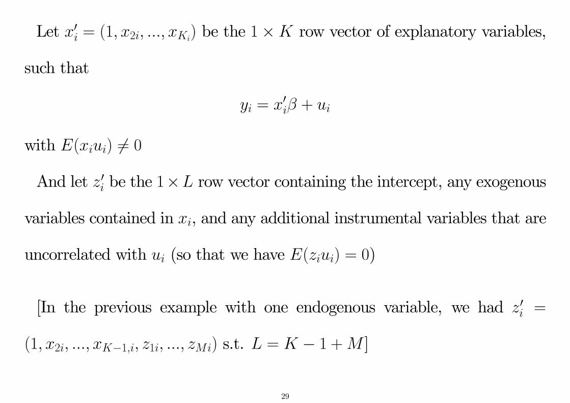
Let x′i = (1, x2i, ..., xKi) be the 1×K row vector of explanatory variables,

such that

yi = x′iβ + ui

with E(xiui) 6= 0

And let z′i be the 1×L row vector containing the intercept, any exogenous

variables contained in xi, and any additional instrumental variables that are

uncorrelated with ui (so that we have E(ziui) = 0)

[In the previous example with one endogenous variable, we had z′i =

(1, x2i, ..., xK−1,i, z1i, ..., zMi) s.t. L = K − 1 + M ]

29

Order condition

L > K

This requires at least as many exogenous variables (including both exoge-

nous explanatory variables and additional instruments) as the number of

parameters we are trying to estimate

- the order condition is necessary but not suffi cient for identification of β

Rank condition

The L×K matrix E(zix′i) has full column rank

rank E(zix′i) = K

- the rank condition is suffi cient for identification of β30

The rank condition can be expressed equivalently as

rank Π = K

in the complete system of first stage equations

X

N ×K

=

,

Z

N × L,

Π

L×K

+

,

R

N ×K

obtained by regressing each element of xi on the row vector z′i

Note that in the special case with K = L = 1, the matrix Π becomes a

scalar, and the rank condition simplifies to the previous requirement that

π 6= 0

31

Example

Consider a model with K = 4

yi = β1 + β2x2i + β3x3i + β4x4i + ui

= x′iβ + ui for i = 1, ..., N

with E(ui) = E(x2iui) = 0 but with E(x3iui) 6= 0 and E(x4iui) 6= 0, so that

E(xiui) = E

ui

x2iui

x3iui

x4iui

=

0

0

E(x3iui)

E(x4iui)

6=

0

0

0

0

32

Suppose we have 3 (additional) instruments that satisfyE(z1iui) = E(z2iui) =

E(z3iui) = 0

Then we have L = 5 and E(ziui) = 0 where z′i is the 1 × 5 vector

(1, x2i, z1i, z2i, z3i), and

E(ziui) = E

ui

x2iui

z1iui

z2iui

z3iui

=

0

0

0

0

0

The complete system of 4 first stage equations is then (for i = 1, ..., N)

33

1 = 1

x2i = x2i

x3i = δ31 + δ32x2i + θ31z1i + θ32z2i + θ33z3i + r3i

x4i = δ41 + δ42x2i + θ41z1i + θ42z2i + θ43z3i + r4i

which can be written as

(1, x2i, x3i, x4i) = (1, x2i, z1i, z2i, z3i)

1 0 δ31 δ41

0 1 δ32 δ42

0 0 θ31 θ41

0 0 θ32 θ42

0 0 θ33 θ43

+ (0, 0, r3i, r4i)

34

or

x′i = z′iΠ + r′i for i = 1, ..., N

where x′i is 1× 4, z′i is 1× 5, Π is 5× 4 and r′i is 1× 4

Stacking across the N observations then gives

X = ZΠ + R

where X is N × 4, Z is N × 5, Π is 5× 4 and R is N × 4

As before, the ith row of X is x′i

Similarly the ith row of Z is z′i, and the ith row of R is r′i

35

Now consider

Π =

1 0 δ31 δ41

0 1 δ32 δ42

0 0 θ31 θ41

0 0 θ32 θ42

0 0 θ33 θ43

The rank condition here requires rank Π = 4

Note that this condition fails if we have either

θ31 = θ32 = θ33 = 0

or θ41 = θ42 = θ43 = 0

36

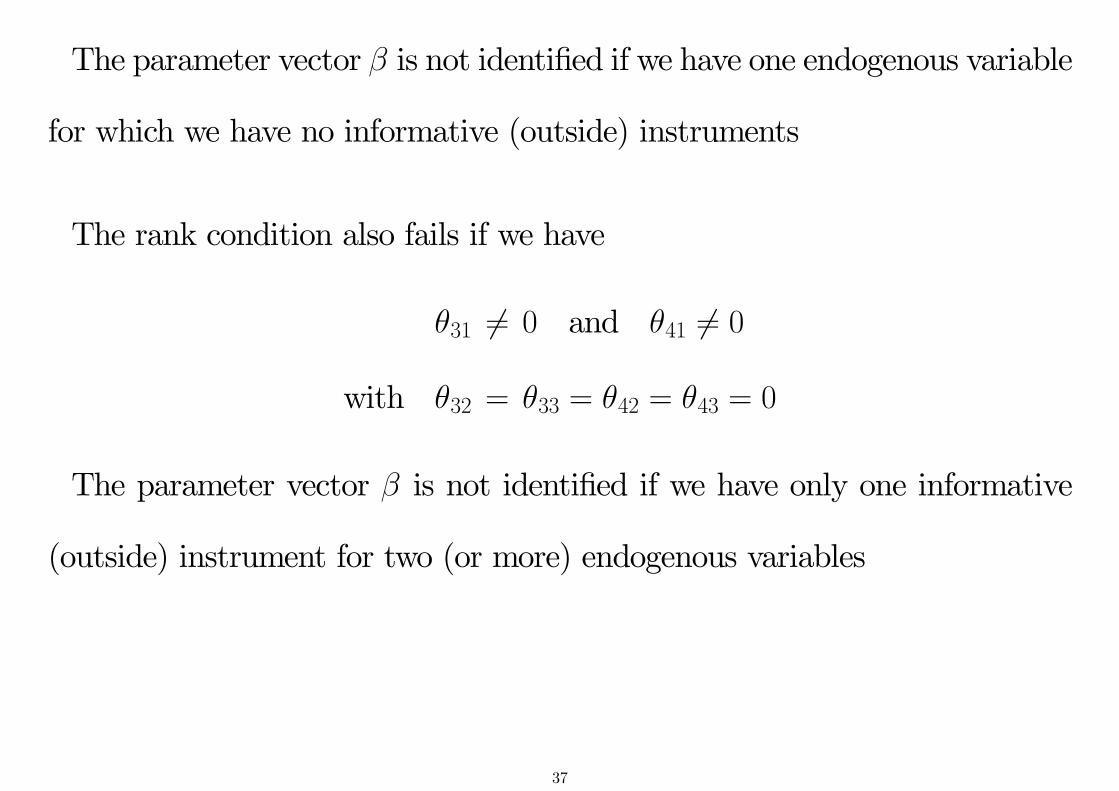
The parameter vector β is not identified if we have one endogenous variable

for which we have no informative (outside) instruments

The rank condition also fails if we have

θ31 6= 0 and θ41 6= 0

with θ32 = θ33 = θ42 = θ43 = 0

The parameter vector β is not identified if we have only one informative

(outside) instrument for two (or more) endogenous variables

37

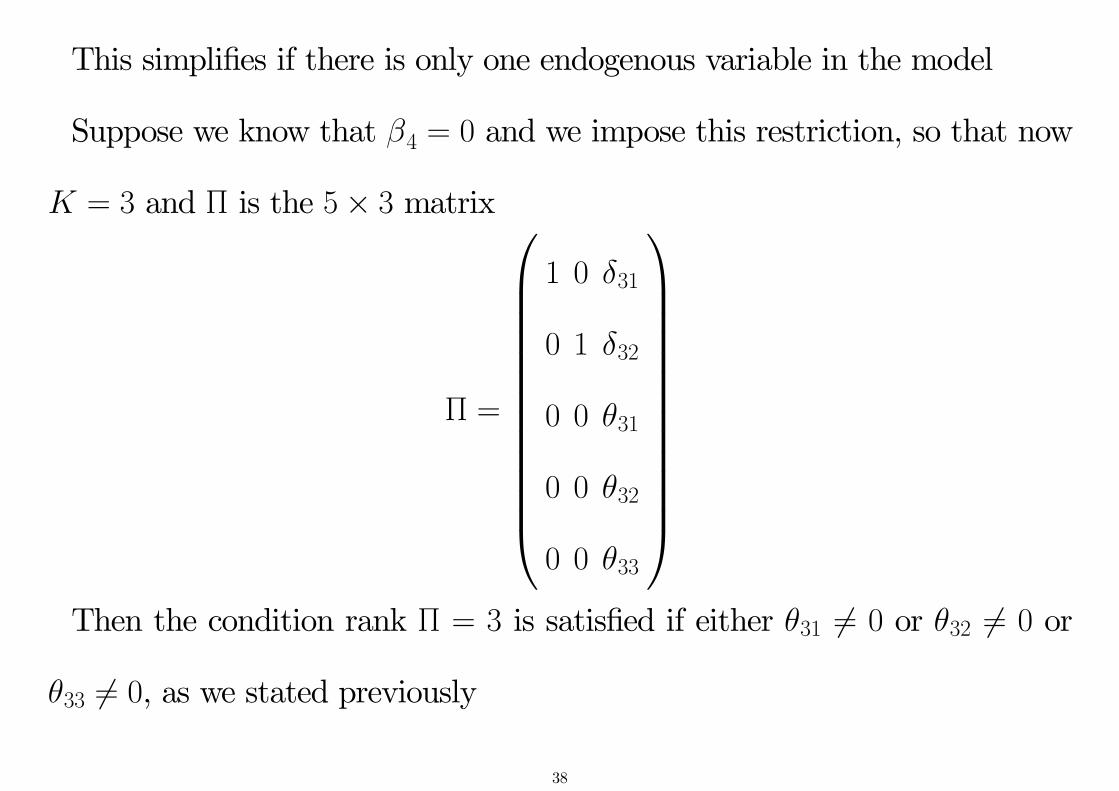
This simplifies if there is only one endogenous variable in the model

Suppose we know that β4 = 0 and we impose this restriction, so that now

K = 3 and Π is the 5× 3 matrix

Π =

1 0 δ31

0 1 δ32

0 0 θ31

0 0 θ32

0 0 θ33

Then the condition rank Π = 3 is satisfied if either θ31 6= 0 or θ32 6= 0 or

θ33 6= 0, as we stated previously

38

The rank condition for identification can in principle be tested, although

statistical tests on the rank of estimated matrices are not trivial, and the

implementation of tests for identification in applications of instrumental vari-

ables is still not common

Inspection of the first stage equations for signs of an identification problem

is good practice and is becoming more common

- given the increasing awareness of finite sample bias problems associated

with ‘weak instruments’or weak identification, that we discuss below

39

Testing over-identifying restrictions

In the just-identified case, whenL = K, theGMMestimator sets 1N

∑Ni=1 ziui

= 0 whether or not the assumption that E(ziui) = 0 is valid, and we cannot

use this fact to test the assumption

In the over-identified case, whenL > K, we can ask whether the minimized

value of the GMM criterion function is ‘small enough’to be consistent with

the validity of our assumption that E(ziui) = 0

This is known as a test of the over-identifying restrictions

40

For the 2SLS estimator in the linear model with conditional homoskedastic-

ity, this test was proposed by Sargan (Econometrica, 1958), and is sometimes

referred to as the Sargan test

For the linear model with conditional heteroskedasticity, and for non-linear

models, this test was generalized for asymptotically effi cient GMM estima-

tors by Hansen (Econometrica, 1982), and is sometimes referred to as the

Hansen test

The link is that 2SLS is the asymptotically effi cient GMM estimator in the

linear model with conditional homoskedasticity

41

[We have not discussed the asymptotically effi cient GMM estimator in the

linear model with conditional heteroskedasticity; you can find details in, for

example, sections 3.4-3.5 of Hayashi (2000)]

42

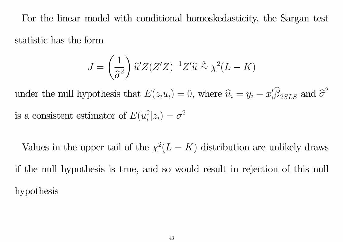
For the linear model with conditional homoskedasticity, the Sargan test

statistic has the form

J =

(1

σ2

)u′Z(Z ′Z)−1Z ′u

a∼ χ2(L−K)

under the null hypothesis that E(ziui) = 0, where ui = yi − x′iβ2SLS and σ2

is a consistent estimator of E(u2i |zi) = σ2

Values in the upper tail of the χ2(L −K) distribution are unlikely draws

if the null hypothesis is true, and so would result in rejection of this null

hypothesis

43

This version of the test of over-identifying restrictions is not robust to

the presence of conditional heteroskedasticity, and should not be used if

conditional heteroskedasticity is suspected

In that case, the heteroskedasticity-robust test of over-identifying restric-

tions proposed by Hansen (1982) can be used

Details can be found in section 3.6 of Hayashi (2000)

44

Testing for endogeneity/simultaneity bias

The motivation for using instrumental variables rather than OLS estima-

tion is that we suspect the OLS estimates would be biased and inconsistent,

as a result of correlation between the error term and one or more of the

explanatory variable(s)

We hope we have used appropriate instruments, and that the 2SLS esti-

mates are consistent, and not subject to important finite sample biases

45

If our instrumental variables are both valid (i.e. uncorrelated with the error

term) and informative (i.e. satisfying the requirements for identification),

then we should expect the 2SLS parameter estimates to be quite different

from the OLS parameter estimates

Comparing these two sets of parameter estimates forms the basis for the

Hausman (Econometrica, 1978) test for (the absence of) endogeneity or si-

multaneity bias

46

The null hypothesis is that there is no correlation between the error term

and all the explanatory variables (i.e. no relevant omitted variables, no

measurement error, ...)

H0 : E(xiui) = 0

The alternative hypothesis is that there is some correlation between the

error term and at least one of the explanatory variables (e.g. due to omitted

variables, measurement error, ...)

H1 : E(xiui) 6= 0

47

H0 : E(xiui) = 0

H1 : E(xiui) 6= 0

To motivate the test, we also assume that we have valid and informative

instrumental variables available under the alternative

Under the null, βOLS is consistent

Under the alternative, βOLS is (biased and) inconsistent, but β2SLS is con-

sistent for some choice of zi 6= xi satisfying E(ziui) = 0 and rank Π = K

48

Under the null, β2SLS is also a consistent estimator of β, although β2SLS

is less effi cient than βOLS if the null hypothesis is valid

- the set of instruments used to obtain β2SLS excludes some of the explana-

tory variables in xi

- given that the null hypothesis is valid, these variables would be both valid

and highly informative instruments, and we lose effi ciency unnecessarily by

not using them

49

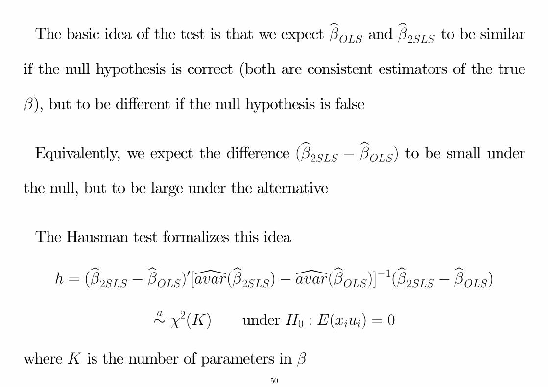
The basic idea of the test is that we expect βOLS and β2SLS to be similar

if the null hypothesis is correct (both are consistent estimators of the true

β), but to be different if the null hypothesis is false

Equivalently, we expect the difference (β2SLS − βOLS) to be small under

the null, but to be large under the alternative

The Hausman test formalizes this idea

h = (β2SLS − βOLS)′[avar(β2SLS)− avar(βOLS)]−1(β2SLS − βOLS)

a∼ χ2(K) under H0 : E(xiui) = 0

where K is the number of parameters in β50

h = (β2SLS − βOLS)′[avar(β2SLS)− avar(βOLS)]−1(β2SLS − βOLS)

Although [avar(β2SLS) − avar(βOLS)] is asymptotically positive definite,

it is possible that we cannot invert our estimate of this covariance matrix in

finite samples

- in this case we can either form a Hausman test statistic based on a subset

of the parameter vector β (typically we focus on the coeffi cients on the

explanatory variables that are treated as endogenous under the alternative),

or use one of the alternative forms of the test discussed, for example, in Chap

6 of Wooldridge, Econometric Analysis of Cross Section and Panel Data51

h = (β2SLS − βOLS)′[avar(β2SLS)− avar(βOLS)]−1(β2SLS − βOLS)

This version of the test is simple to compute, but requires E(u2i |zi) = σ2,

and is not robust to conditional heteroskedasticity

The simplicity follows from the conditional homoskedasticity assumption,

under which βOLS is asymptotically effi cient under the null hypothesis, and

avar(β2SLS − βOLS) simplifies to [avar(β2SLS)− avar(βOLS)]

Alternative, heteroskedasticity-robust versions of the test are available, and

are discussed, for example, in Chapter 6 of Wooldridge, Econometric Analy-

sis of Cross Section and Panel Data52

Finite sample problems

Instrumental variables estimators like 2SLS are consistent if the instru-

ments used are both valid and informative, but they may be subject to

important finite sample biases

We now look at two distinct sources of finite sample bias

- the use of ‘too many’instruments relative to the available sample size

- the use of instruments that are only weakly related to the endogenous

variable(s), resulting in ‘weak identification’of the parameters of interest

53

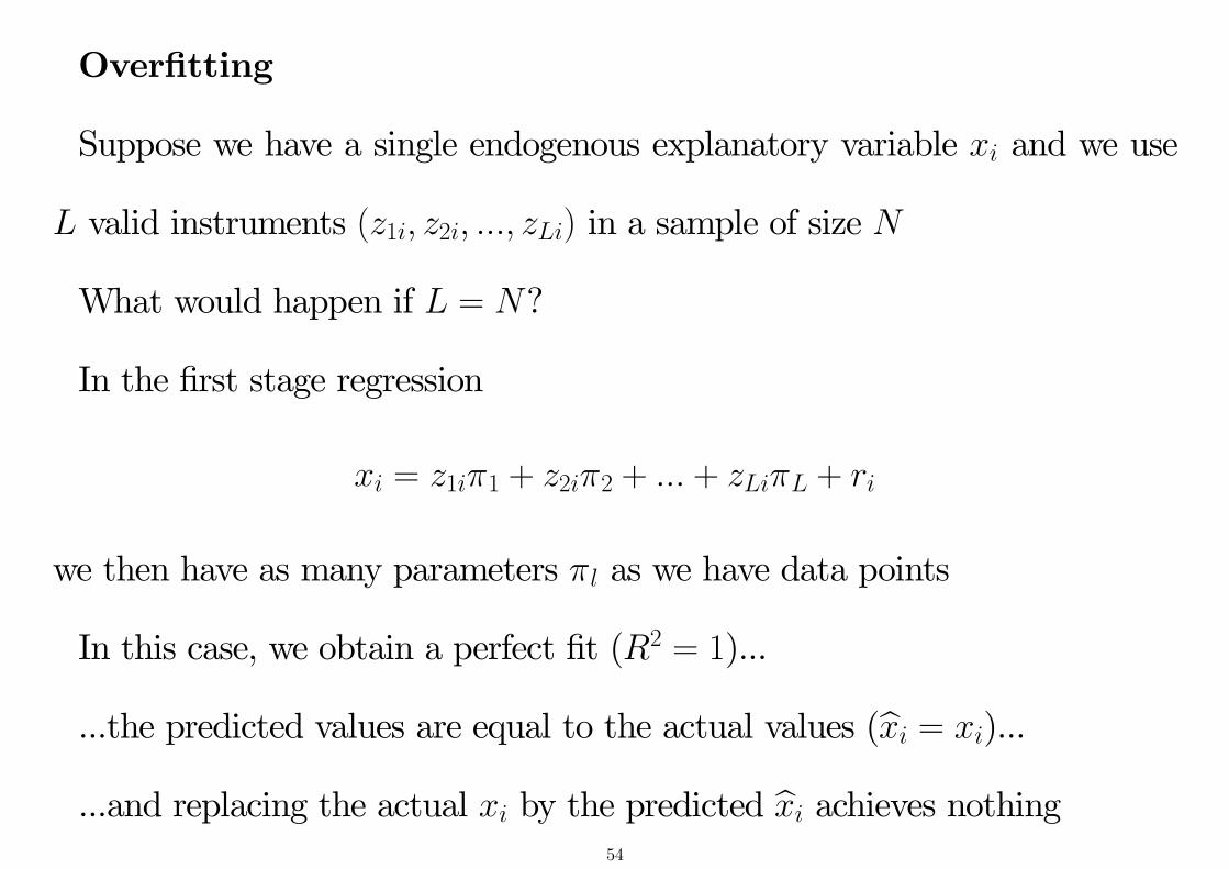
Overfitting

Suppose we have a single endogenous explanatory variable xi and we use

L valid instruments (z1i, z2i, ..., zLi) in a sample of size N

What would happen if L = N?

In the first stage regression

xi = z1iπ1 + z2iπ2 + ... + zLiπL + ri

we then have as many parameters πl as we have data points

In this case, we obtain a perfect fit (R2 = 1)...

...the predicted values are equal to the actual values (xi = xi)...

...and replacing the actual xi by the predicted xi achieves nothing54

In this case the second stage regression coincides with the standard OLS

regression: β2SLS = βOLS

β2SLS will therefore have exactly the same bias as βOLS

While no-one would use this many instruments in practice, a similar finite

sample bias occurs in less extreme circumstances

As the number of instruments (L) approaches the sample size (N), the

2SLS estimator β2SLS tends towards the OLS estimator βOLS

Since the OLS estimator is expected to be biased, the 2SLS estimator may

also have a serious finite sample bias (in the direction of the OLS estimator)

if ‘too many’instruments are used relative to the sample size - even though

all the instruments are valid55

Thus if we find that β2SLS and βOLS are similar, we should check that

this is not the result of using ‘too many’instruments, before concluding that

there is no inconsistency in the OLS estimates

One simple way to investigate this is to calculate a sequence of 2SLS esti-

mates based on smaller and smaller subsets of the original instruments

- and check that there is no systematic tendency for the 2SLS estimates to

move away from the OLS estimates, in a particular direction, as we reduce

the dimension of the instrument set

Moral - avoid the temptation to use ‘too many’instruments, particularly

when this results in precise 2SLS estimates that are close to their OLS coun-

terpart56

Weak instruments

‘Weak instruments’describes the situation where the instruments used only

weakly identify the parameters of interest

When there is a single instrument for a single endogenous variable, this cor-

responds to the instrument being only weakly correlated with the endogenous

variable

Weak identification is an important concern in many contexts

This introduces two distinct problems, depending on whether the weak

instruments are strictly valid instruments, or not57

i) finite sample bias

We first assume the instruments used are strictly valid (E(ziui) = 0), in

which case the 2SLS estimator is consistent if the parameters are formally

identified

Still there can be an important finite sample bias if the instruments provide

very little (additional) information about the endogenous variable(s)

To explore this, we focus on the model with one endogenous variable and

one instrument, and consider the extreme case in which the instrument is

completely uninformative (s.t. β is not identified)

58

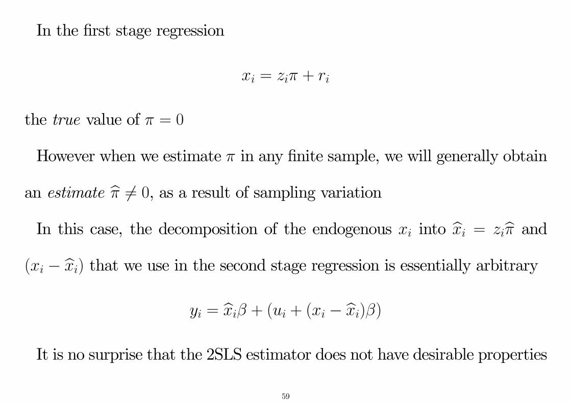
In the first stage regression

xi = ziπ + ri

the true value of π = 0

However when we estimate π in any finite sample, we will generally obtain

an estimate π 6= 0, as a result of sampling variation

In this case, the decomposition of the endogenous xi into xi = ziπ and

(xi − xi) that we use in the second stage regression is essentially arbitrary

yi = xiβ + (ui + (xi − xi)β)

It is no surprise that the 2SLS estimator does not have desirable properties

59

In this case, the distribution of the 2SLS estimator has the same expected

value as the OLS estimator - see Bound, Jaeger and Baker, Journal of the

American Statistical Association, 1995

[The two estimators do not coincide in this case; the 2SLS estimator will

have much higher variance than the corresponding OLS estimator]

More generally, when the instruments used are valid in the sense of being

uncorrelated with ui, but only weakly correlated with xi, β2SLS can have an

important finite sample bias in the direction of βOLS

If the instruments used are weak enough, even sample sizes that appear

enormous are not suffi cient to eliminate the possibility of quantitatively im-

portant finite sample biases60

ii) large inconsistency

The second problem associated with weak instruments is that any inconsis-

tency of β2SLS, which will be present if the instruments have some correlation

with ui, gets magnified if the instruments are also only weakly correlated

with xi

Intuition may suggest that the bias of 2SLS should be lower than the bias

of OLS, if the correlation between the error term and the instruments is

much lower than the correlation between the error term and the endogenous

variable(s)

61

This intuition can be seriously wrong in situtations where the instru-

ments are only weakly correlated with the explanatory variable(s)

To see this, recall that in the case of a single explanatory variable we have

p limN→∞

βOLS = β + p limN→∞

(X ′X

N

)−1

p limN→∞

(X ′u

N

)

= β +p limN→∞

(X ′uN

)p limN→∞

(X ′XN

)

62

Also recall that in the case of a single explanatory variable we have

p limN→∞

β2SLS = β + p limN→∞

(X ′X

N

)−1

p limN→∞

(X ′u

N

)

= β +p limN→∞

(X ′uN

)p limN→∞

(X ′XN

)

63

Now compare

p limN→∞

βOLS = β +p limN→∞

(X ′uN

)p limN→∞

(X ′XN

)and p lim

N→∞β2SLS = β +

p limN→∞

(X ′uN

)p limN→∞

(X ′XN

)A high covariance between xi and ui could translate into a modest incon-

sistency for βOLS if the variance of xi is suffi ciently large

While a small covariance between xi and ui could translate into a large

inconsistency for β2SLS if the covariance between xi and xi is also very small

The latter is relevant when the instruments zi are onlyweakly correlated

with xi (i.e. when xi = z′iπ with π ≈ 0)64

Morals

- avoid using weak instruments whenever possible

- avoid attaching too much significance to 2SLS estimates in situations

where the best available instruments are nevertheless very weak

- look carefully at the first stage regression equations relating the endoge-

nous xi variables to the instruments (and any exogenous xi variables) to check

whether the (additional) instruments have reasonable explanatory power for

each of the endogenous variables

65

- for discussion of some suggested diagnostic tests, see Bound, Jaeger and

Baker (JASA, 1995) and the discussions in Chapter 5 of Wooldridge, Econo-

metric Analysis of Cross Section and Panel Data or Chapter 4 of Cameron

and Trivedi, Microeconometrics: Methods and Applications

The latest version of the ivreg2 command in Stata now implements a num-

ber of these suggestions

66