KISSsoft 03/2016 – Instruction 068a

Sizing of Topological Modification of Bevel Gears

KISSsoft AG

Uetzikon 4

8634 Hombrechtikon

Switzerland

Tel: +41 55 254 20 50

Fax: +41 55 254 20 51

info@KISSsoft.AG

www.KISSsoft.AG

05.10.2016 2 / 20

Contents

Introduction ........................................................................................................................................................................................ 3

Calculation instruction .................................................................................................................................................................. 3

2.1 User interface ....................................................................................................................................................................... 3

2.2 Calculation settings ........................................................................................................................................................... 4

2.2.1 Tooth thickness.............................................................................................................................................................. 4

2.2.2 Standard format of measurement data ............................................................................................................. 5

2.2.3 Validity of the measurement data ........................................................................................................................ 6

2.2.4 Applying calculated topological modifications ............................................................................................... 7

2.3 Auxiliary settings ................................................................................................................................................................ 7

2.3.1 2D tooth form calculation .......................................................................................................................................... 7

2.3.2 Settings for 3D geometry generation ................................................................................................................. 8

Calculation procedure and results......................................................................................................................................... 9

3.1.1 Convergence criteria ................................................................................................................................................... 9

3.1.2 Error messages ............................................................................................................................................................. 9

Calculation Examples ............................................................................................................................................................... 11

4.1 An example for Klingelnberg ............................................................. Fehler! Textmarke nicht definiert.

4.2 An example for Gleason ...................................................................... Fehler! Textmarke nicht definiert.

4.3 An example for Zeiss ............................................................................ Fehler! Textmarke nicht definiert.

References ............................................................................................................................................................................................... 11

Annex 1 ...................................................................................................................................................................................................... 12

An approach of pairing bevel gears from conventional cutting machine with gears produced on 5-axis

milling machine ...................................................................................................................................................................................... 12

05.10.2016 3 / 20

Introduction This instruction explains the background and the usage of the topological modification calculation for

bevel gears. In order to use the calculation, experience on the 3D model generation in KISSsoft is pre-

requisite. Please refer to [1] for the detailed instruction for generating 3D geometry of bevel gear.

Calculation instruction

2.1 User interface

The calculation is available under the menu Calculation > Topological modifications. Figure 1 shows the

calculation window.

Figure 1 Input window for topological modification calculation

(1) The “Measurement machine” selects the format of the measurement data file. There four

different types are available [Klingelnberg, Gleason, TBevel (Klingelnberg), TBevel (Gleason),

Zeiss]. Here, the TBevel® types are the measurement report format from Wenzel [ 2 ] for

Klingelnberg and Gleason machine. You should be very careful when you import the

measurement grid data not to mix up the types and/or gears and/or flanks. Otherwise, the

program will generate an error message.

(2) The “Maximum no. of iterations” sets the maximum number of iteration steps during the

calculation. If the calculation doesn’t converge until the maximum iterations, the calculation will

stop and you will find the message in the report “NOT CONVERGED: Maximum iterations

reached”.

(3) The “Convergence tolerance” sets the maximum deviation between the given measurement

data and the 3D geometry model with the topological modification. The deviation is defined as

the minimum Euclidean distance between the given grid point to the modified surface.

(4) The “Permissible number of points outside the tolerance” sets the allowable number of

points having bigger deviation than the convergence tolerance. For example, in some cases,

only one or two points are exceeding the tolerance and blocks the program to converge. In that

case, it’s better to ignore these points if the points are from measurement noise.

05.10.2016 4 / 20

(5) The “Measurement data” sets the full path of the measurement data files to be used as a target

flank surface. In order to follow the convention, the Klingelnberg type machine has separate files

for the right and the left flank, while Gleason and Zeiss machines have both flanks data in a

single file.

(6) The “Remove edge points in the measurement data” option is used to ignore the edge points

(at tooth ends and tip diameter) in the measurement data during the calculation. Refer to 2.2.2

for details.

(7) The “Gear” shows if the measurement data is for pinion or gear. This is determined from the

measurement data.

(8) The “Data format” shows the actual data format of the defined measurement data by checking

the coordinate system of the data. If the data format is conflicting with the setting of

“Measurement machine”, the program will use the actual data format. However, it’s always

recommended to check if your setting is correct, when you have the conflict.

(9) The “Number of columns” and “Number of rows” shows the data determined from the

measurement data report.

(10) The “Tooth thickness modification coefficient” is calculated to give initial tooth thickness

modification from the given measurement data. If you accept the calculated value, the program

will proceed with the proposed value for the calculation. Otherwise, it will proceed with the

original tooth thickness modification coefficient. Refer to 2.2.1 for details.

(11) You can do the calculation by the “Calculate” button. When the calculation finishes, whatever

it’s converged or not, the “Save” and “Report” buttons are activated enabling to check the report.

The “Report” button shows the deviation and the modification values for each steps with the

convergence result. It also contains description of the reason for the error when it happens. The

“Save” button saves the last step of the calculated topological modification for each flank,

whatever the calculation converged or not. By default, the saved file has the name of “User

defined name”+Gear1RF.dat for right flank of gear 1 and “User defined name”+Gear1LF.dat for

left flank of gear 1. The “Accept” button is activated only after you saved the modification

template. When you accept the result, the proposed tooth thickness modification coefficient (if

you applied) and the topological modification templates are transferred to the main calculation

file. In this case, all the previous modifications of the corresponding gear will be removed.

2.2 Calculation settings

2.2.1 Tooth thickness

KISSsoft does not allow negative values for the topological modification meaning that it does not allow

to increase the tooth thickness by the modification and works as the way of removing the material from

the initial model. Thus, the initial tooth thickness of the model should be big enough to completely cover

the target tooth flank. The user can increase the tooth thickness either by changing the tooth thickness

tolerance or by changing the tooth thickness modification coefficient. However, it’s recommended to set

the tooth thickness tolerance to no backlash condition and then change only the thickness modification

coefficient for simpler handling.

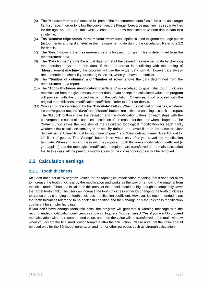
If you don’t have enough tooth thickness, the program will generate a warning message with the

recommended modification coefficient as shown in Figure 2. You can select ‘Yes’ if you want to proceed

the calculation with the recommended value, and then the value will be transferred to the main window

when you accept the final modification template after the calculation. Please note that the value should

be used only for the 3D model generation and not for other purposes such as strength calculation.

05.10.2016 5 / 20

Figure 2 Warning message for tooth thickness modification coefficient

2.2.2 Standard format of measurement data

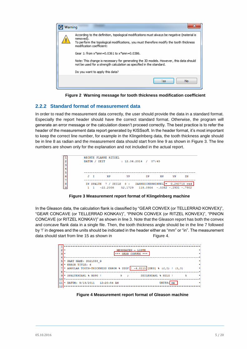
In order to read the measurement data correctly, the user should provide the data in a standard format.

Especially the report header should have the correct standard format. Otherwise, the program will

generate an error message or the calculation doesn’t proceed correctly. The best practice is to refer the

header of the measurement data report generated by KISSsoft. In the header format, it’s most important

to keep the correct line number, for example in the Klingelnberg data, the tooth thickness angle should

be in line 8 as radian and the measurement data should start from line 9 as shown in Figure 3. The line

numbers are shown only for the explanation and not included in the actual report.

Figure 3 Measurement report format of Klingelnberg machine

In the Gleason data, the calculation flank is classified by “GEAR CONVEX (or TELLERRAD KONVEX)”,

“GEAR CONCAVE (or TELLERRAD KONKAV)”, “PINION CONVEX (or RITZEL KONVEX)”, “PINION

CONCAVE (or RITZEL KONKAV)” as shown in line 3. Note that the Gleason report has both the convex

and concave flank data in a single file. Then, the tooth thickness angle should be in the line 7 followed

by ‘!’ in degrees and the units should be indicated in the header either as “mm” or “in”. The measurement

data should start from line 15 as shown in Figure 4.

Figure 4 Measurement report format of Gleason machine

05.10.2016 6 / 20

2.2.3 Validity of the measurement data

The calculation is using numerical optimization process based on the deviation between the given

measurement data and the 3D model from KISSsoft. Thus, it can generate an error during the calculation

caused from the original measurement data. So, you should note the following points very carefully.

(1) The calculation assumes the measurement data is defined for the nominal flank. Thus the data

including the points outside the nominal flank, it’s giving an error and stops the calculation.

(2) If the measurement data are highly irregular, the calculation may suffer from the convergence and

give an error.

(3) When calculating the deviation, we add boundary values on the edges (side I and side II of the face

width and at the root form and the tip diameters) automatically to calculation the modification

template. The edge values are generated from linear extrapolation from the neighboring

measurement data. Thus, if the given measurement data have the values close to the edges, it’s

prone to give an error during the calculation.

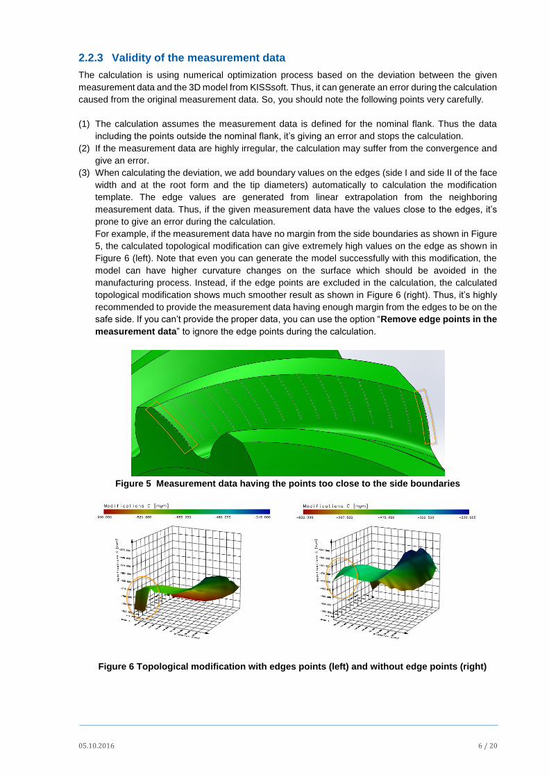
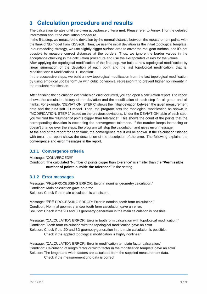
For example, if the measurement data have no margin from the side boundaries as shown in Figure

5, the calculated topological modification can give extremely high values on the edge as shown in

Figure 6 (left). Note that even you can generate the model successfully with this modification, the

model can have higher curvature changes on the surface which should be avoided in the

manufacturing process. Instead, if the edge points are excluded in the calculation, the calculated

topological modification shows much smoother result as shown in Figure 6 (right). Thus, it’s highly

recommended to provide the measurement data having enough margin from the edges to be on the

safe side. If you can’t provide the proper data, you can use the option “Remove edge points in the

measurement data” to ignore the edge points during the calculation.

Figure 5 Measurement data having the points too close to the side boundaries

Figure 6 Topological modification with edges points (left) and without edge points (right)

05.10.2016 7 / 20

(4) In addition, the calculation is based on the assumption that the reference point is positioned at the

middle of the face width. The possible reason for this is that the measurement data have different

margins on side I and II. In this case, the program is not working properly and need a new data

having same margins and therefore the reference point is positioned at the middle of face width.

Figure 7 Margins for measurement data should be same at both sides

2.2.4 Applying calculated topological modifications

The topological modification calculation ignores the any type of predefined modifications during the

calculation. When you accept the result, the proposed tooth thickness modification coefficient (if you

applied) and the topological modification templates are added to the main calculation file with the

corresponding link to the saved template file. Note that all the predefined modifications of the

corresponding gear will be deactivated.

Figure 8 Definition of the topological modification

2.3 Auxiliary settings

2.3.1 2D tooth form calculation

In order to generate the 3D geometry of bevel gear, KISSsoft calculates the 2D tooth forms at predefined

sections along the face width. Then, the 2D tooth forms are approximated to the spline curves to be

used for 3D geometry generation. We are using “Quadratic spline” as a default approximation type, but

it’s recommended to use “Cubic spline” for the topological modification calculation especially when you

are suffering from the tooth form calculation error. You can change the setting in the tab “Tooth form”

as shown in Figure 9.

Figure 9 Settings for 2D tooth form calculation

05.10.2016 8 / 20

Figure 10 shows an example for the topological modification to be applied, and you can see that the

modification surface is highly nonlinear. Thus, the tooth form cannot be easily approximated by quadratic

spline and the topological modification calculation often suffers from the tooth form calculation.

Figure 10 An example of topological modification

2.3.2 Settings for 3D geometry generation

Several settings for 3D geometry generation also affects the calculation and the result. You can find the

setting in the Module specific settings window as shown in Figure 11.

Figure 11 Settings for 3D geometry generation

The “Number of sections along face width” defines the number of sections to calculate the tooth form

for the approximation of tooth flank form. The minimum value is 3, and the default value is 11. Normally,

the quality of the final model can be increased with increasing the value, but it’s not recommended to

use excessively many sections compared with the tooth dimension. However, if the measurement data

has higher number of columns, for example 15x15, it’s recommended to use bigger number of sections

than the columns.

The “Modeling operation tolerance” sets the tolerance for internal operations of 3D geometry

generation process by Parasolid® kernel such as crash detection in Boolean operation or checking the

intersection between objects. The default value is 1m. You don’t need to change the value for the

topological modification calculation in most cases, except the 3D model cannot be generated even

without the modification.

05.10.2016 9 / 20

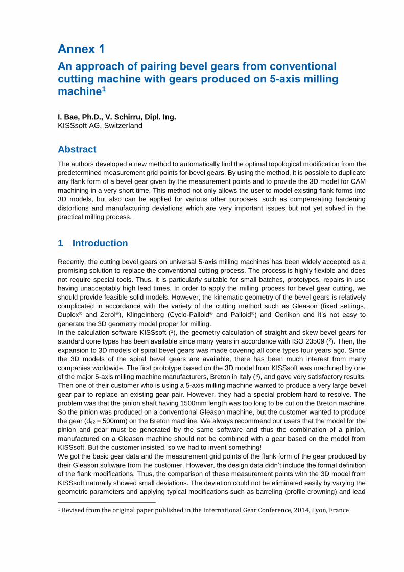
Calculation procedure and results The calculation iterates until the given acceptance criteria met. Please refer to Annex 1 for the detailed

information about the calculation procedure.

In the first step, we measure the deviation by the normal distance between the measurement points with

the flank of 3D model from KISSsoft. Then, we use the initial deviation as the initial topological template.

In our modeling strategy, we use slightly bigger surface area to cover the real gear surface, and it’s not

possible to measure correct distances at the borders. Thus, we ignore the border values in the

acceptance checking in the calculation procedure and use the extrapolated values for the values.

After applying the topological modification of the first step, we build a new topological modification by

linear summation of the deviation of each point and the last topological modification, that is,

Modification2 = Modification1 + Deviation1.

In the successive steps, we build a new topological modification from the last topological modification

by using empirical update formula with cubic polynomial regression fit to prevent higher nonlinearity in

the resultant modification.

After finishing the calculation even when an error occurred, you can open a calculation report. The report

shows the calculation history of the deviation and the modification of each step for all gears and all

flanks. For example, “DEVIATION: STEP 0” shows the initial deviation between the given measurement

data and the KISSsoft 3D model. Then, the program sets the topological modification as shown in

“MODIFICATION: STEP 1” based on the previous deviations. Under the DEVIATION table of each step,

you will find the “Number of points bigger than tolerance”. This shows the count of the points that the

corresponding deviation is exceeding the convergence tolerance. If the number keeps increasing or

doesn’t change over the steps, the program will stop the calculation and gives error message.

At the end of the report for each flank, the convergence result will be shown. If the calculation finished

with error, the report shows the description of the description of the error. The following explains the

convergence and error messages in the report.

3.1.1 Convergence criteria

Message: “CONVERGED!!!”

Condition: The calculated “Number of points bigger than tolerance” is smaller than the “Permissible

number of points outside the tolerance” in the setting.

3.1.2 Error messages

Message: “PRE-PROCESSING ERROR: Error in nominal geometry calculation.”

Condition: Main calculation gave an error.

Solution: Check if the main calculation is consistent.

Message: “PRE-PROCESSING ERROR: Error in nominal tooth form calculation.”

Condition: Nominal geometry and/or tooth form calculation gave an error.

Solution: Check if the 2D and 3D geometry generation in the main calculation is possible.

Message: “CALCULATION ERROR: Error in tooth form calculation with topological modification.”

Condition: Tooth form calculation with the topological modification gave an error.

Solution: Check if the 2D and 3D geometry generation in the main calculation is possible.

Check if the applied topological modification is highly nonlinear.

Message: “CALCULATION ERROR: Error in modification template factor calculation.”

Condition: Calculation of length factor or width factor in the modification template gave an error.

Solution: The length and width factors are calculated from the supplied measurement data.

Check if the measurement grid data is correct.

05.10.2016 10 / 20

Message: “CALCULATION ERROR: Error in the topological modification calculation.”

Condition: Calculation of the deviation of the modified surface gave an error.

Solution: Check if the deviation or the topological modification is highly nonlinear or too big.

Check if the tooth thickness modification factor is set reasonably.

Message: “NOT CONVERGED: Maximum iteration steps reached”

Condition: Maximum number of iterations reached

Solution: Increase the maximum number of iterations.

Increase the “Convergence tolerance”.

Increase the “Permissible number of points outside the tolerance”

Message: “NOT CONVERGED: Last three steps have same deviation”

Condition: The deviation values are not updated any more in last three steps.

Solution: Check if the deviation is having negative value or too big.

Check if the dimension of the gear and the measurement grid data is correct.

Check if the thickness modification factor is set reasonably.

Message: “NOT CONVERGED: Number of points bigger than tolerance increasing in last five steps”

Condition: The calculation is diverging.

Solution: Check if the deviation is having negative value or too big.

Check if the dimension of the gear and the measurement grid data is correct.

Check if the thickness modification factor is set reasonably.

Message: “FILE READING ERROR”

Condition: Reading measurement data report gives an error.

Solution: Check if the measurement data has wrong format.

05.10.2016 11 / 20

Calculation Examples Please contact to support@kisssoft.ch for more information.

References

[1] KISSsoft 03/2014 – Instruction 068, 3D Geometry of Bevel Gears

[2] http://www.wenzel-group.com/praezision/de/produkte/software/uebersicht/kmgsoftware.php

Annex 1

An approach of pairing bevel gears from conventional cutting machine with gears produced on 5-axis milling machine1

I. Bae, Ph.D., V. Schirru, Dipl. Ing. KISSsoft AG, Switzerland

Abstract

The authors developed a new method to automatically find the optimal topological modification from the

predetermined measurement grid points for bevel gears. By using the method, it is possible to duplicate

any flank form of a bevel gear given by the measurement points and to provide the 3D model for CAM

machining in a very short time. This method not only allows the user to model existing flank forms into

3D models, but also can be applied for various other purposes, such as compensating hardening

distortions and manufacturing deviations which are very important issues but not yet solved in the

practical milling process.

1 Introduction

Recently, the cutting bevel gears on universal 5-axis milling machines has been widely accepted as a

promising solution to replace the conventional cutting process. The process is highly flexible and does

not require special tools. Thus, it is particularly suitable for small batches, prototypes, repairs in use

having unacceptably high lead times. In order to apply the milling process for bevel gear cutting, we

should provide feasible solid models. However, the kinematic geometry of the bevel gears is relatively

complicated in accordance with the variety of the cutting method such as Gleason (fixed settings,

Duplex® and Zerol®), Klingelnberg (Cyclo-Palloid® and Palloid®) and Oerlikon and it’s not easy to

generate the 3D geometry model proper for milling.

In the calculation software KISSsoft (1), the geometry calculation of straight and skew bevel gears for

standard cone types has been available since many years in accordance with ISO 23509 (2). Then, the

expansion to 3D models of spiral bevel gears was made covering all cone types four years ago. Since

the 3D models of the spiral bevel gears are available, there has been much interest from many

companies worldwide. The first prototype based on the 3D model from KISSsoft was machined by one

of the major 5-axis milling machine manufacturers, Breton in Italy (3), and gave very satisfactory results.

Then one of their customer who is using a 5-axis milling machine wanted to produce a very large bevel

gear pair to replace an existing gear pair. However, they had a special problem hard to resolve. The

problem was that the pinion shaft having 1500mm length was too long to be cut on the Breton machine.

So the pinion was produced on a conventional Gleason machine, but the customer wanted to produce

the gear (de2 = 500mm) on the Breton machine. We always recommend our users that the model for the

pinion and gear must be generated by the same software and thus the combination of a pinion,

manufactured on a Gleason machine should not be combined with a gear based on the model from

KISSsoft. But the customer insisted, so we had to invent something!

We got the basic gear data and the measurement grid points of the flank form of the gear produced by

their Gleason software from the customer. However, the design data didn’t include the formal definition

of the flank modifications. Thus, the comparison of these measurement points with the 3D model from

KISSsoft naturally showed small deviations. The deviation could not be eliminated easily by varying the

geometric parameters and applying typical modifications such as barreling (profile crowning) and lead

1 Revised from the original paper published in the International Gear Conference, 2014, Lyon, France

05.10.2016 13 / 20

crowning. Thus, we developed a creative solution to generate a 3D model of the gear from KISSsoft and

to adapt it to the given grid point from Gleason. In the following chapters, we will show the procedure of

the method and the application results.

Topological modification of the 3D Model

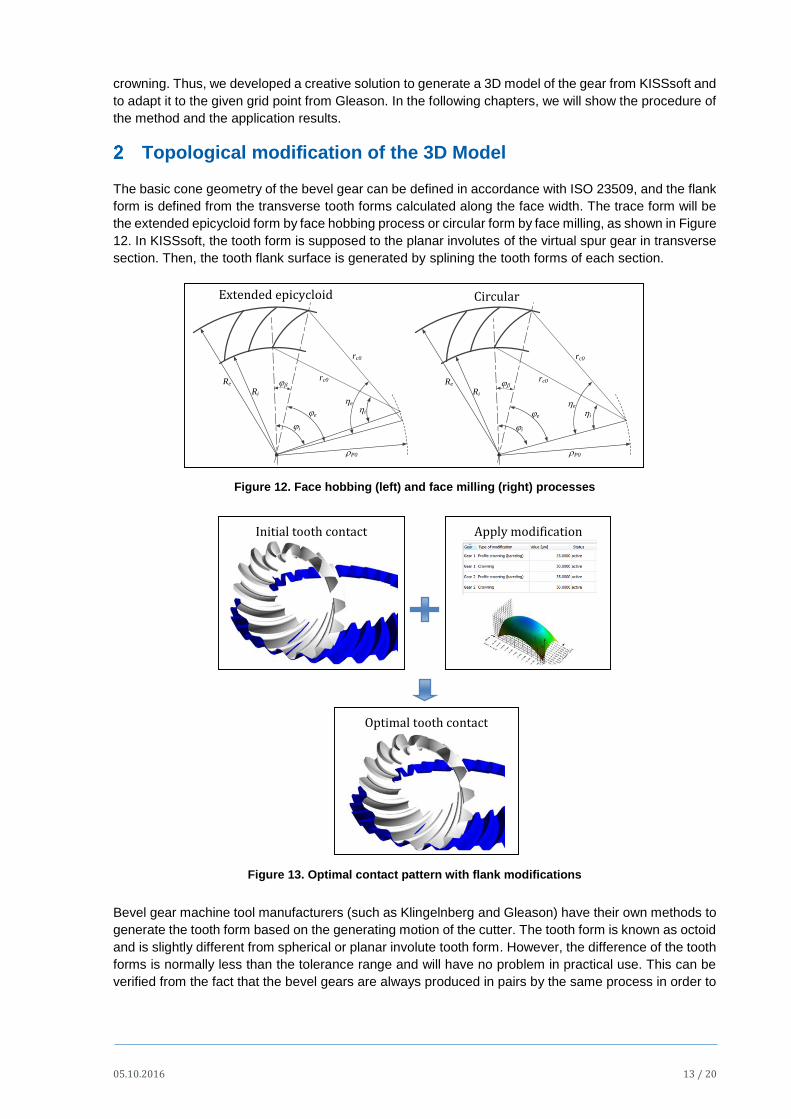
The basic cone geometry of the bevel gear can be defined in accordance with ISO 23509, and the flank

form is defined from the transverse tooth forms calculated along the face width. The trace form will be

the extended epicycloid form by face hobbing process or circular form by face milling, as shown in Figure

12. In KISSsoft, the tooth form is supposed to the planar involutes of the virtual spur gear in transverse

section. Then, the tooth flank surface is generated by splining the tooth forms of each section.

Figure 12. Face hobbing (left) and face milling (right) processes

Figure 13. Optimal contact pattern with flank modifications

Bevel gear machine tool manufacturers (such as Klingelnberg and Gleason) have their own methods to

generate the tooth form based on the generating motion of the cutter. The tooth form is known as octoid

and is slightly different from spherical or planar involute tooth form. However, the difference of the tooth

forms is normally less than the tolerance range and will have no problem in practical use. This can be

verified from the fact that the bevel gears are always produced in pairs by the same process in order to

Re

Ri

jb

ji

jehi

he

rP0

rc0

rc0

Re

Ri

jb

ji

je hi

he

rP0

rc0

rc0

Initial tooth contact

Optimal tooth contact

Apply modification

Extended epicycloid Circular

05.10.2016 14 / 20

achieve a good contact pattern in practice. In order to validate the practical usage of the 3D model from

KISSsoft, we compared our model with reference models of manufacturer programs and also carried

out the contact pattern check with the actual model. The result showed the tooth flanks along the face

width of the two models are very well matched with only slight differences (4).

It’s one of the most important tasks to find the optimal modification to give good contact pattern in a

bevel gear pair. In KISSsoft, the contact pattern of the bevel gear pair can be easily optimized by using

proper modifications as shown in Figure 13. There are eight types of the modifications available for

bevel gears in KISSsoft (profile crowning, eccentric profile crowning, pressure angle modification, helix

angle modification, lead crowning, eccentric lead crowning, twist, and topological modification). The user

can define different combination of modifications for drive and coast flanks to optimize the contact

pattern separately.

However, if the target modification has highly non-linear or irregular pattern, the simple combination of

the conventional modifications cannot be applied. In that case, the topological modification should be

used to allow the user to freely define any type of modification that can’t be covered by the conventional

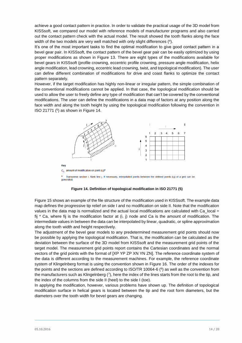
modifications. The user can define the modifications in a data map of factors at any position along the

face width and along the tooth height by using the topological modification following the convention in

ISO 21771 (5) as shown in Figure 14.

Figure 14. Definition of topological modification in ISO 21771 (5)

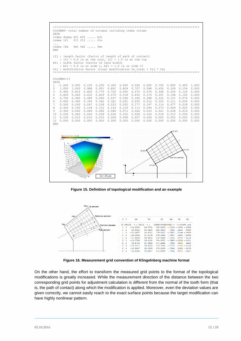
Figure 15 shows an example of the file structure of the modification used in KISSsoft. The example data

map defines the progressive tip relief on side I and no modification on side II. Note that the modification

values in the data map is normalized and the actual local modifications are calculated with Ca_local =

fij * Ca, where fij is the modification factor at (i, j) node and Ca is the amount of modification. The

intermediate values in between the data can be interpolated by linear, quadratic, or spline approximation

along the tooth width and height respectively.

The adjustment of the bevel gear models to any predetermined measurement grid points should now

be possible by applying the topological modification. That is, the modification can be calculated as the

deviation between the surface of the 3D model from KISSsoft and the measurement grid points of the

target model. The measurement grid points report contains the Cartesian coordinates and the normal

vectors of the grid points with the format of [XP YP ZP XN YN ZN]. The reference coordinate system of

the data is different according to the measurement machines. For example, the reference coordinate

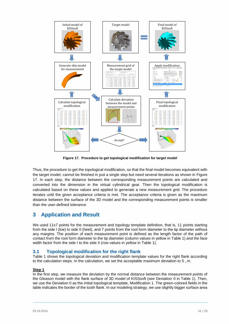
system of Klingelnberg format is using the convention shown in Figure 16. The order of the indexes for

the points and the sections are defined according to ISO/TR 10064-6 (6) as well as the convention from

the manufacturers such as Klingelnberg (7), here the index of the lines starts from the root to the tip, and

the index of the columns from the side II (heel) to the side I (toe).

In applying the modification, however, various problems have shown up. The definition of topological

modification surface in helical gears is located between the tip and the root form diameters, but the

diameters over the tooth width for bevel gears are changing.

05.10.2016 15 / 20

Figure 15. Definition of topological modification and an example

Figure 16. Measurement grid convention of Klingelnberg machine format

On the other hand, the effort to transform the measured grid points to the format of the topological

modifications is greatly increased. While the measurement direction of the distance between the two

corresponding grid points for adjustment calculation is different from the normal of the tooth form (that

is, the path of contact) along which the modification is applied. Moreover, even the deviation values are

given correctly, we cannot easily reach to the exact surface points because the target modification can

have highly nonlinear pattern.

**************************************************************************************

COLUMNS= total number of columns including index column

DATA

index dummy bf1 bf2 ..... bfn

index lf1 f11 f12 ..... f1n

...

index lfm fm1 fm2 ..... fmn

END

lfj : length factor (factor of length of path of contact)

: lfj = 0.0 is at the root, lfj = 1.0 is at the tip

bfi : width factor (factor of face width)

: bfi = 0.0 is on side I, bfi = 1.0 is on side II

fij : modification factor (local modification Ca_local = fij * Ca)

**************************************************************************************

COLUMNS=13

DATA

1 -1.000 0.000 0.100 0.200 0.300 0.400 0.500 0.600 0.700 0.800 0.900 1.000

2 1.000 1.000 0.988 0.951 0.891 0.809 0.707 0.588 0.454 0.309 0.156 0.000

3 0.900 0.810 0.800 0.770 0.722 0.655 0.573 0.476 0.368 0.250 0.126 0.000

4 0.800 0.640 0.632 0.609 0.570 0.518 0.452 0.376 0.291 0.198 0.100 0.000

5 0.700 0.490 0.484 0.466 0.437 0.396 0.346 0.288 0.222 0.151 0.076 0.000

6 0.600 0.360 0.356 0.342 0.321 0.291 0.255 0.212 0.163 0.111 0.056 0.000

7 0.500 0.250 0.247 0.238 0.223 0.202 0.177 0.147 0.114 0.077 0.039 0.000

8 0.400 0.160 0.158 0.152 0.143 0.129 0.113 0.094 0.073 0.049 0.025 0.000

9 0.300 0.090 0.089 0.086 0.080 0.073 0.064 0.053 0.041 0.028 0.014 0.000

10 0.200 0.040 0.040 0.038 0.036 0.032 0.028 0.024 0.018 0.012 0.006 0.000

11 0.100 0.010 0.010 0.010 0.009 0.008 0.007 0.006 0.005 0.003 0.002 0.000

12 0.000 0.000 0.000 0.000 0.000 0.000 0.000 0.000 0.000 0.000 0.000 0.000

END

Ca = 25 m

05.10.2016 16 / 20

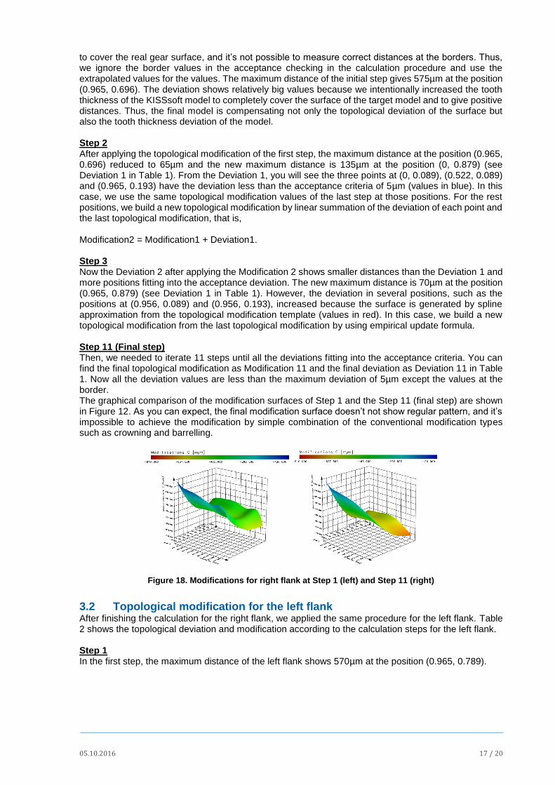
Figure 17. Procedure to get topological modification for target model

Thus, the procedure to get the topological modification, so that the final model becomes equivalent with

the target model, cannot be finished in just a single step but need several iterations as shown in Figure

17. In each step, the distance between the corresponding measurement points are calculated and

converted into the dimension in the virtual cylindrical gear. Then the topological modification is

calculated based on these values and applied to generate a new measurement grid. The procedure

iterates until the given acceptance criteria is met. The acceptance criteria is given as the maximum

distance between the surface of the 3D model and the corresponding measurement points is smaller

than the user-defined tolerance.

3 Application and Result

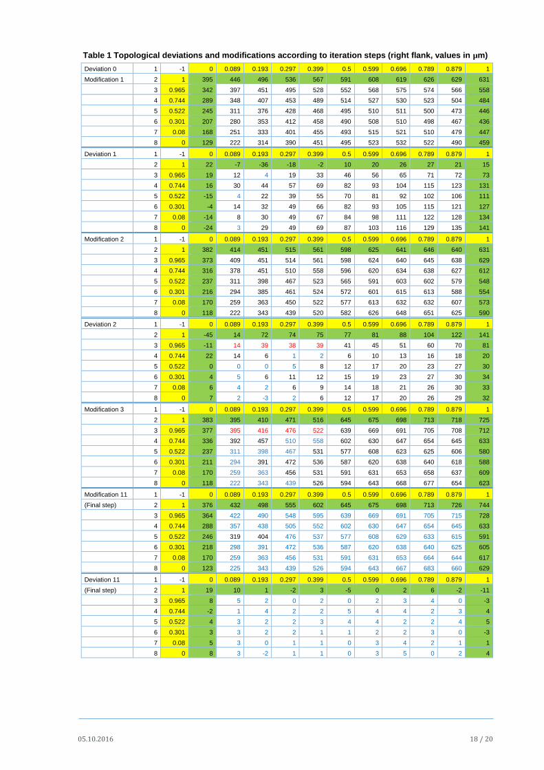
We used 11x7 points for the measurement and topology template definition, that is, 11 points starting from the side I (toe) to side II (heel), and 7 points from the root form diameter to the tip diameter without any margins. The position of each measurement point is defined as the length factor of the path of contact from the root form diameter to the tip diameter (column values in yellow in Table 1) and the face width factor from the side I to the side II (row values in yellow in Table 1).

3.1 Topological modification for the right flank Table 1 shows the topological deviation and modification template values for the right flank according to the calculation steps. In the calculation, we set the acceptable maximum deviation to 5 m. Step 1 In the first step, we measure the deviation by the normal distance between the measurement points of the Gleason model with the flank surface of 3D model of KISSsoft (see Deviation 0 in Table 1). Then, we use the Deviation 0 as the initial topological template, Modification 1. The green-colored fields in the table indicates the border of the tooth flank. In our modeling strategy, we use slightly bigger surface area

Initial model of KISSsoft

Target model

Generate skin model for measurement

Measurement grid of the target model

Calculate deviation between the model and

measurement points

Accept?

Calculate topological modification

Final model of KISSsoft

Final topological modification

Apply modification

05.10.2016 17 / 20

to cover the real gear surface, and it’s not possible to measure correct distances at the borders. Thus, we ignore the border values in the acceptance checking in the calculation procedure and use the extrapolated values for the values. The maximum distance of the initial step gives 575µm at the position (0.965, 0.696). The deviation shows relatively big values because we intentionally increased the tooth thickness of the KISSsoft model to completely cover the surface of the target model and to give positive distances. Thus, the final model is compensating not only the topological deviation of the surface but also the tooth thickness deviation of the model. Step 2 After applying the topological modification of the first step, the maximum distance at the position (0.965, 0.696) reduced to 65µm and the new maximum distance is 135µm at the position (0, 0.879) (see Deviation 1 in Table 1). From the Deviation 1, you will see the three points at (0, 0.089), (0.522, 0.089) and (0.965, 0.193) have the deviation less than the acceptance criteria of 5µm (values in blue). In this case, we use the same topological modification values of the last step at those positions. For the rest positions, we build a new topological modification by linear summation of the deviation of each point and the last topological modification, that is, Modification2 = Modification1 + Deviation1. Step 3 Now the Deviation 2 after applying the Modification 2 shows smaller distances than the Deviation 1 and more positions fitting into the acceptance deviation. The new maximum distance is 70µm at the position (0.965, 0.879) (see Deviation 1 in Table 1). However, the deviation in several positions, such as the positions at (0.956, 0.089) and (0.956, 0.193), increased because the surface is generated by spline approximation from the topological modification template (values in red). In this case, we build a new topological modification from the last topological modification by using empirical update formula. Step 11 (Final step) Then, we needed to iterate 11 steps until all the deviations fitting into the acceptance criteria. You can find the final topological modification as Modification 11 and the final deviation as Deviation 11 in Table 1. Now all the deviation values are less than the maximum deviation of 5µm except the values at the border. The graphical comparison of the modification surfaces of Step 1 and the Step 11 (final step) are shown in Figure 12. As you can expect, the final modification surface doesn’t not show regular pattern, and it’s impossible to achieve the modification by simple combination of the conventional modification types such as crowning and barrelling.

Figure 18. Modifications for right flank at Step 1 (left) and Step 11 (right)

3.2 Topological modification for the left flank After finishing the calculation for the right flank, we applied the same procedure for the left flank. Table 2 shows the topological deviation and modification according to the calculation steps for the left flank. Step 1 In the first step, the maximum distance of the left flank shows 570µm at the position (0.965, 0.789).

05.10.2016 18 / 20

Table 1 Topological deviations and modifications according to iteration steps (right flank, values in µm)

Deviation 0 1 -1 0 0.089 0.193 0.297 0.399 0.5 0.599 0.696 0.789 0.879 1

Modification 1 2 1 395 446 496 536 567 591 608 619 626 629 631

3 0.965 342 397 451 495 528 552 568 575 574 566 558

4 0.744 289 348 407 453 489 514 527 530 523 504 484

5 0.522 245 311 376 428 468 495 510 511 500 473 446

6 0.301 207 280 353 412 458 490 508 510 498 467 436

7 0.08 168 251 333 401 455 493 515 521 510 479 447

8 0 129 222 314 390 451 495 523 532 522 490 459

Deviation 1 1 -1 0 0.089 0.193 0.297 0.399 0.5 0.599 0.696 0.789 0.879 1

2 1 22 -7 -36 -18 -2 10 20 26 27 21 15

3 0.965 19 12 4 19 33 46 56 65 71 72 73

4 0.744 16 30 44 57 69 82 93 104 115 123 131

5 0.522 -15 4 22 39 55 70 81 92 102 106 111

6 0.301 -4 14 32 49 66 82 93 105 115 121 127

7 0.08 -14 8 30 49 67 84 98 111 122 128 134

8 0 -24 3 29 49 69 87 103 116 129 135 141

Modification 2 1 -1 0 0.089 0.193 0.297 0.399 0.5 0.599 0.696 0.789 0.879 1

2 1 382 414 451 515 561 598 625 641 646 640 631

3 0.965 373 409 451 514 561 598 624 640 645 638 629

4 0.744 316 378 451 510 558 596 620 634 638 627 612

5 0.522 237 311 398 467 523 565 591 603 602 579 548

6 0.301 216 294 385 461 524 572 601 615 613 588 554

7 0.08 170 259 363 450 522 577 613 632 632 607 573

8 0 118 222 343 439 520 582 626 648 651 625 590

Deviation 2 1 -1 0 0.089 0.193 0.297 0.399 0.5 0.599 0.696 0.789 0.879 1

2 1 -45 14 72 74 75 77 81 88 104 122 141

3 0.965 -11 14 39 38 39 41 45 51 60 70 81

4 0.744 22 14 6 1 2 6 10 13 16 18 20

5 0.522 0 0 0 5 8 12 17 20 23 27 30

6 0.301 4 5 6 11 12 15 19 23 27 30 34

7 0.08 6 4 2 6 9 14 18 21 26 30 33

8 0 7 2 -3 2 6 12 17 20 26 29 32

Modification 3 1 -1 0 0.089 0.193 0.297 0.399 0.5 0.599 0.696 0.789 0.879 1

2 1 383 395 410 471 516 645 675 698 713 718 725

3 0.965 377 395 416 476 522 639 669 691 705 708 712

4 0.744 336 392 457 510 558 602 630 647 654 645 633

5 0.522 237 311 398 467 531 577 608 623 625 606 580

6 0.301 211 294 391 472 536 587 620 638 640 618 588

7 0.08 170 259 363 456 531 591 631 653 658 637 609

8 0 118 222 343 439 526 594 643 668 677 654 623

Modification 11 1 -1 0 0.089 0.193 0.297 0.399 0.5 0.599 0.696 0.789 0.879 1

(Final step) 2 1 376 432 498 555 602 645 675 698 713 726 744

3 0.965 364 422 490 548 595 639 669 691 705 715 728

4 0.744 288 357 438 505 552 602 630 647 654 645 633

5 0.522 246 319 404 476 537 577 608 629 633 615 591

6 0.301 218 298 391 472 536 587 620 638 640 625 605

7 0.08 170 259 363 456 531 591 631 653 664 644 617

8 0 123 225 343 439 526 594 643 667 683 660 629

Deviation 11 1 -1 0 0.089 0.193 0.297 0.399 0.5 0.599 0.696 0.789 0.879 1

(Final step) 2 1 19 10 1 -2 3 -5 0 2 6 -2 -11

3 0.965 8 5 2 0 2 0 2 3 4 0 -3

4 0.744 -2 1 4 2 2 5 4 4 2 3 4

5 0.522 4 3 2 2 3 4 4 2 2 4 5

6 0.301 3 3 2 2 1 1 2 2 3 0 -3

7 0.08 5 3 0 1 1 0 3 4 2 1 1

8 0 8 3 -2 1 1 0 3 5 0 2 4

05.10.2016 19 / 20

Table 2. Topological deviations and modifications according to iteration steps (left flank, values in µm)

Deviation 0 1 -1 0 0.089 0.193 0.297 0.399 0.5 0.599 0.696 0.789 0.879 1

Modification 1 2 1 110 199 287 365 434 493 538 568 578 569 559

3 0.965 145 225 306 375 438 490 531 558 570 564 558

4 0.744 181 252 324 386 441 488 524 549 561 559 556

5 0.522 219 281 344 397 444 484 515 537 548 549 549

6 0.301 269 320 372 416 454 487 513 531 541 543 545

7 0.08 342 382 423 456 486 511 531 544 552 555 559

8 0 415 444 473 497 518 535 548 557 563 568 572

Deviation 1 1 -1 0 0.089 0.193 0.297 0.399 0.5 0.599 0.696 0.789 0.879 1

2 1 63 62 60 63 67 70 77 87 105 120 135

3 0.965 34 38 43 53 63 73 84 96 112 125 138

4 0.744 4 15 27 44 59 77 92 106 119 130 141

5 0.522 33 38 43 53 63 75 87 100 114 127 140

6 0.301 35 40 46 57 68 80 91 105 118 132 145

7 0.08 65 66 66 73 81 90 100 113 126 140 154

8 0 95 91 87 90 94 100 109 121 135 149 163

Modification 2 1 -1 0 0.089 0.193 0.297 0.399 0.5 0.599 0.696 0.789 0.879 1

2 1 188 262 349 428 501 563 615 654 682 689 698

3 0.965 189 263 349 428 501 563 615 654 682 689 698

4 0.744 195 267 351 430 500 565 616 655 680 689 701

5 0.522 261 319 387 450 507 559 602 637 662 676 695

6 0.301 310 360 418 473 522 567 604 636 659 675 697

7 0.08 413 448 489 529 567 601 631 657 678 695 718

8 0 514 535 560 587 612 635 657 678 698 717 743

Deviation 2 1 -1 0 0.089 0.193 0.297 0.399 0.5 0.599 0.696 0.789 0.879 1

2 1 49 33 16 -2 1 16 30 36 36 34 32

3 0.965 27 20 12 3 5 14 22 27 30 31 33

4 0.744 6 7 7 7 9 11 14 18 23 28 33

5 0.522 6 6 6 7 9 11 15 19 24 28 33

6 0.301 1 3 5 8 11 15 18 22 26 30 35

7 0.08 18 17 16 15 16 18 21 25 29 34 39

8 0 35 31 27 23 21 21 23 27 33 39 44

Modification 3 1 -1 0 0.089 0.193 0.297 0.399 0.5 0.599 0.696 0.789 0.879 1

2 1 218 284 361 427 500 577 638 682 713 720 730

3 0.965 216 283 361 428 501 577 637 681 712 720 731

4 0.744 202 274 358 437 509 576 630 673 703 717 736

5 0.522 267 325 393 457 516 570 617 656 686 704 728

6 0.301 310 360 418 481 533 582 622 658 685 705 732

7 0.08 431 465 505 544 583 619 652 682 707 729 759

8 0 548 566 587 610 633 656 680 705 731 756 790

Modification 14 1 -1 0 0.089 0.193 0.297 0.399 0.5 0.599 0.696 0.789 0.879 1

(Final step) 2 1 158 241 337 427 506 577 638 682 713 728 747

3 0.965 166 246 340 428 506 577 637 681 712 727 747

4 0.744 211 279 358 437 509 576 630 673 703 723 750

5 0.522 267 325 393 457 516 570 617 656 686 710 742

6 0.301 310 360 418 481 533 582 622 658 690 712 742

7 0.08 436 474 518 546 583 619 652 682 714 738 770

8 0 554 579 608 610 633 655 675 709 740 767 803

Deviation 14 1 -1 0 0.089 0.193 0.297 0.399 0.5 0.599 0.696 0.789 0.879 1

(Final step) 2 1 2 1 0 0 -1 2 5 6 5 0 -4

3 0.965 0 1 2 1 1 2 3 4 4 1 -3

4 0.744 -1 1 4 2 3 2 2 2 3 1 -2

5 0.522 6 4 1 0 2 3 4 5 5 1 -4

6 0.301 2 3 4 2 2 3 3 4 2 2 1

7 0.08 6 3 1 3 4 3 4 5 2 3 3

8 0 11 4 -3 5 5 3 5 5 2 4 5

05.10.2016 20 / 20

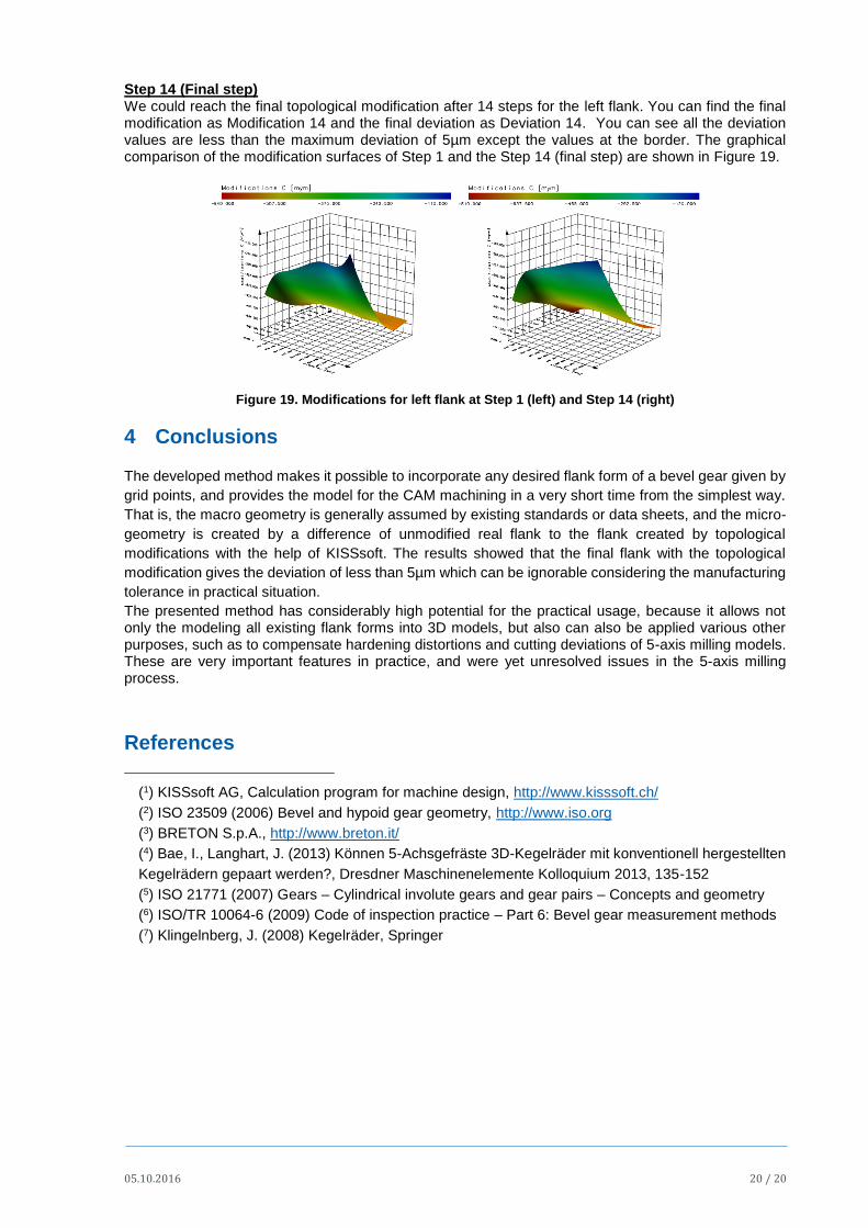
Step 14 (Final step) We could reach the final topological modification after 14 steps for the left flank. You can find the final modification as Modification 14 and the final deviation as Deviation 14. You can see all the deviation values are less than the maximum deviation of 5µm except the values at the border. The graphical comparison of the modification surfaces of Step 1 and the Step 14 (final step) are shown in Figure 19.

Figure 19. Modifications for left flank at Step 1 (left) and Step 14 (right)

4 Conclusions

The developed method makes it possible to incorporate any desired flank form of a bevel gear given by

grid points, and provides the model for the CAM machining in a very short time from the simplest way.

That is, the macro geometry is generally assumed by existing standards or data sheets, and the micro-

geometry is created by a difference of unmodified real flank to the flank created by topological

modifications with the help of KISSsoft. The results showed that the final flank with the topological

modification gives the deviation of less than 5µm which can be ignorable considering the manufacturing

tolerance in practical situation.

The presented method has considerably high potential for the practical usage, because it allows not only the modeling all existing flank forms into 3D models, but also can also be applied various other purposes, such as to compensate hardening distortions and cutting deviations of 5-axis milling models. These are very important features in practice, and were yet unresolved issues in the 5-axis milling process.

References

(1) KISSsoft AG, Calculation program for machine design, http://www.kisssoft.ch/

(2) ISO 23509 (2006) Bevel and hypoid gear geometry, http://www.iso.org

(3) BRETON S.p.A., http://www.breton.it/

(4) Bae, I., Langhart, J. (2013) Können 5-Achsgefräste 3D-Kegelräder mit konventionell hergestellten

Kegelrädern gepaart werden?, Dresdner Maschinenelemente Kolloquium 2013, 135-152

(5) ISO 21771 (2007) Gears – Cylindrical involute gears and gear pairs – Concepts and geometry

(6) ISO/TR 10064-6 (2009) Code of inspection practice – Part 6: Bevel gear measurement methods

(7) Klingelnberg, J. (2008) Kegelräder, Springer