institutional investment constraints and stock prices€¦ · regulations, contract requirements,...
TRANSCRIPT

JOURNAL OF FINANCIAL AND QUANTITATIVE ANALYSIS Vol. 52, No. 2, Apr. 2017, pp. 465–489COPYRIGHT 2017, MICHAEL G. FOSTER SCHOOL OF BUSINESS, UNIVERSITY OF WASHINGTON, SEATTLE, WA 98195doi:10.1017/S0022109017000102
Institutional Investment Constraints andStock Prices
Jie Cao, Bing Han, and Qinghai Wang*
AbstractWe test the hypothesis that investment constraints in delegated portfolio management maydistort demand for stocks, leading to price underreaction to news and stock return pre-dictability. We find that institutions tend not to buy more of a stock with good news thatthey already overweight; they are reluctant to sell a stock with bad news that they alreadyunderweight. Stocks with good news overweighted by institutions subsequently signifi-cantly outperform stocks with bad news underweighted by institutions. The impact of in-stitutional investment constraints sheds new light on asset pricing anomalies such as stockprice momentum and post–earnings announcement drift.
I. Introduction
One of the most significant changes in the financial market has been thesurge of delegated portfolio management. Increasing portions of U.S. equitiesare managed by institutional investors such as pension funds and mutual funds.Institutional investors are different from individual investors and face a variety ofconstraints in their investment decisions. These constraints include restrictions onthe market capitalization and the style of stocks in the portfolio, position lim-its on a stock or an industry, and restrictions on the tracking errors, portfolioturnover, and investment strategies allowed. Such constraints arise as a product of
*Cao, [email protected], Business School, Chinese University of Hong Kong; Han (correspond-ing author), [email protected], Rotman School of Management, University of Toronto,and Shanghai Advanced Institute of Finance, Shanghai Jiao Tong University; and Wang, [email protected], College of Business Administration, University of Central Florida. We thank StephenBrown (the editor), Aydogan Alti, Michael Brennan, John Griffin, Jean Helwege, David Hirshleifer,Kewei Hou, Jennifer Huang, Hao Jiang (the referee), Jonathan Lewellen, Stefan Nagel, Laura Starks,Rene Stulz, Michael Stutzer, Siew-Hong Teoh, Sheridan Titman, Ralph Walkling, Russ Wermers, LuZheng, and seminar participants at the Hong Kong University of Science and Technology, PekingUniversity, Ohio State University, the University of Texas at Austin, the 2007 Financial ManagementAssociation Meetings, and the 2005 Western Finance Association Meetings for helpful discussionsand comments. All remaining errors are our own. The work described in this paper was partially sup-ported by a grant from the Research Grant Council of the Hong Kong Special Administrative Region,China (Project No. CUHK 458212).
465
https://doi.org/10.1017/S0022109017000102D
ownloaded from
https://ww
w.cam
bridge.org/core . IP address: 54.191.40.80 , on 20 Aug 2017 at 02:23:22 , subject to the Cambridge Core term
s of use, available at https://ww
w.cam
bridge.org/core/terms .
466 Journal of Financial and Quantitative Analysis
regulations, contract requirements, and agency considerations in delegated port-folio management (e.g., Almazan, Brown, Carlson, and Chapman (2004)).
This paper studies the implications of institutional investment constraints forstock demand and valuation. Investment constraints may limit institutional in-vestors’ ability to transfer their information into portfolio positions. Institutionscould even ignore their own information and “go with the flow” (e.g., Maug andNaik (2011)). This dampened response to information may induce price under-reaction for stocks that are affected by institutional investment constraints andgenerate cross-sectional return predictability as the mispricing subsequently getscorrected.
To empirically measure institutional investment constraints and conduct testsof their impact on institutions’ trading and stock prices, we focus on two sets ofimportant institutional investment constraints that are common yet have not beenwell researched in the literature. The first is the diversification requirement. TheInvestment Company Act of 1940 explicitly requires that mutual funds must meetvarious investment diversification standards to qualify for “diversified” status andfavorable tax treatment. The Employee Retirement Income Security Act of 1974(ERISA) requires that pension funds “diversify investments . . . so as to minimizethe risk of large losses, unless under the circumstances it is clearly prudent notto do so.”1 Civil legal penalties can be imposed on fiduciaries in a lawsuit forviolation of ERISA’s diversification requirements. In such lawsuits, defendantsbear the burden of showing that the decision not to diversify was clearly prudent.
Institutional investors often are subject to both explicit and implicit tracking-error constraints in their investment decisions. The explicit tracking-errorconstraint as specified in investment contracts restricts the maximal possible devi-ation of a money manager’s portfolio from a given benchmark. Violation of suchconstraints can result in contract termination and lawsuits.2 Even without the con-tractual tracking-error constraint, portfolio managers have increasingly empha-sized the risk of underperforming a benchmark index. The risk of being wrongand alone, popularly recognized as the “maverick risk,” is viewed as the great-est peril in investment management by many practitioners (Arnott (2003)). Thetracking-error restriction is the second type of institutional investment constraintthat motivates our study.
The combination of diversification requirements and tracking-error restric-tions could lead to institutional investment decisions that are otherwise diffi-cult to explain. Recent studies document that institutions are reluctant to deviatefrom the market portfolio or the benchmark they are expected to beat (e.g.,Lakonishok, Shleifer, and Vishny (1997), Chan, Chen, and Lakonishok (2002),Cohen, Gompers, and Vuolteenaho (2002), Cremers and Petajisto (2009), andLewellen (2011)). Such “benchmark investing” contradicts predictions of neo-classic models: Institutional investors are usually viewed as being better informed
1See Section 404 of ERISA. Although ERISA established the guidelines for private pension planadministration and investment practices, the general guidelines are widely adopted by public pensionfunds, bank trusts, and, to a large extent, mutual funds (see O’Barr and Conley (1992)).
2See, for example, Pensions & Investments (May 12, 2003), which reports that Merrill LynchInvestment Managers was accused of breaching tracking-error limits on its equities mandate and paid75 million pounds in settlement.
https://doi.org/10.1017/S0022109017000102D
ownloaded from
https://ww
w.cam
bridge.org/core . IP address: 54.191.40.80 , on 20 Aug 2017 at 02:23:22 , subject to the Cambridge Core term
s of use, available at https://ww
w.cam
bridge.org/core/terms .

Cao, Han, and Wang 467
than individual investors. Thus, they should overweight stocks that have positivenews and underweight stocks with negative news. However, because of diversifi-cation requirements and tracking-error restrictions, money managers tend to holdlarge, diversified portfolios that closely mimic the market portfolio (or their pol-icy/performance benchmark). Thus, they may not fully take advantage of theirinformation in their investment decisions. For example, Cohen et al. (2002) esti-mate that institutions capture only about a third of the gains that they could if theybought more of the stocks they rated as winners and sold more of the ones theyrated as losers.
This paper provides further evidence that institutional investment constraintsaffect money managers’ demand for stocks and trading behavior. Because of di-versification requirements and tracking-error constraints, institutions cannot orwill not keep deviating from their benchmarks. We hypothesize that if moneymanagers already overweight a stock, they may not buy more of the stock evenif they receive positive information about the stock. If money managers alreadyunderweight a stock, they may be reluctant to sell the stock even if they receivenegative information about the stock. Such investment behavior may affect thevaluation of stocks and generate testable return patterns.
Our basic hypothesis on the asset pricing implication of institutional invest-ment constraints can be illustrated with an example. Suppose institutions receivea positive signal about a stock, but they already overweight this stock. When in-vestment constraints become binding (e.g., the signal or the overweight is largeenough), then institutions’ demand schedule for the stock will not shift up by asmuch as it would without the investment constraints. In other words, their demandfor the stock at a given price would be lower than the benchmark case without theinvestment constraints. When the demand curve for stock is downward sloping,stock with good news that is already overweighted by the institutions would havea lower market-clearing price than the case without the investment constraints. Inthis sense, the stock is undervalued because the good news is not fully reflectedin the market price, thus setting the scene for higher future returns. Similarly, in-stitutions may be constrained from selling stocks that they already underweighteven when they have negative information about the stocks. Thus, stocks with badnews that are underweighted by the institutions are overvalued (because the badnews is not fully reflected in the market price) and would have abnormally lowfuture returns.
The impact of investment constraints on stock prices generates cross-sectional differences in stock returns that depend on both the direction of institu-tional investment constraints and the signs of informational signals. For example,when institutions receive good news about a stock, institutions’ buying constraintsare more likely to be binding if they already overweight the stock than if they un-derweight it. Thus, among stocks that have good news, those stocks currentlyoverweighted by institutions would experience more price underreactions and de-liver higher future returns than those stocks currently underweighted by institu-tions. Similarly, institutions would have more constraints in selling a stock withbad news if they already underweight it. Thus, among stocks that are experienc-ing bad news, those stocks currently underweighted by institutions tend to sub-sequently underperform those currently overweighted by institutions. Finally, for
https://doi.org/10.1017/S0022109017000102D
ownloaded from
https://ww
w.cam
bridge.org/core . IP address: 54.191.40.80 , on 20 Aug 2017 at 02:23:22 , subject to the Cambridge Core term
s of use, available at https://ww
w.cam
bridge.org/core/terms .

468 Journal of Financial and Quantitative Analysis
stocks without significant news, institutional investment constraints should havelittle impact on stock prices. Thus, no significant differences are expected in thefuture returns of stocks that institutions currently overweight and those they un-derweight when the stocks do not have significant news.
Using quarterly data on institutional equity holdings between 1980 and 2013,we construct two measures of institutional investment constraints for each stockand in each quarter. We compute the fraction of institutions that overweight thestock and the abnormal level of aggregate institutional ownership of the stock.The overweight and underweight measures capture the essence of diversificationrequirements and tracking-error restrictions. We use two proxies for news, onebased on stock returns over a relatively short horizon (e.g., 6 months) and theother based on the firm’s quarterly earnings surprises.
We find direct evidence that investment constraints affect institutional trad-ing behavior. Institutions are reluctant to buy stocks they already overweight orsell stocks they already underweight. More importantly, empirical tests stronglysupport our hypotheses on the asset pricing impact of institutional investment con-straints. Among stocks that have good news, those that institutions already over-weight subsequently significantly outperform those that institutions underweight.Similarly, for stocks that have bad news, those that institutions underweight subse-quently underperform those that institutions overweight. Our results are consistentacross all combinations of constraint measures and information proxies.
Our tests reveal interesting interactions between institutional investment con-straints and well-known asset pricing anomalies such as stock price momentumand post–earnings announcement drift. For example, we find that a refined mo-mentum strategy that buys only the winner stocks that the institutions overweightand shorts the loser stocks that the institutions underweight is significantly moreprofitable than the simple momentum strategy that buys all past winners and shortsall past losers. We also find stronger post–earnings announcement drifts for stocksexperiencing greater institutional investment constraints.
To the extent that momentum and post–earnings announcement drifts man-ifest mispricing caused by behavioral-biased investors and institutional investorsare the “smart money,” our findings are also consistent with the idea that in-stitutional investors’ investment constraints limit their ability to arbitrage stockmispricing.3 Our main argument is that when institutional investors already sig-nificantly overweight or underweight a stock, their investment constraints preventthem from fully utilizing their information advantage. Such information advan-tage could be about firm fundamentals or stock valuations.
Several recent studies rely on the details of mutual fund holdings to predictstock returns and interpret the findings as evidence of mutual fund managers’ in-formation advantage (e.g., Cohen, Polk, and Silli (2010), Wermers, Yao, and Zhao(2012), and Jiang, Verbeek, and Wang (2014)). These studies show that certainvariables constructed from mutual fund holdings can predict stock returns in un-conditional tests, whereas our hypotheses are conditional on information proxies.Our paper complements and extends these studies. Our results are consistent
3Lewellen (2011) provides evidence that institutions’ investment decisions are constrained by thelimits of arbitrage considerations.
https://doi.org/10.1017/S0022109017000102D
ownloaded from
https://ww
w.cam
bridge.org/core . IP address: 54.191.40.80 , on 20 Aug 2017 at 02:23:22 , subject to the Cambridge Core term
s of use, available at https://ww
w.cam
bridge.org/core/terms .

Cao, Han, and Wang 469
with their conclusion that money managers can possess private information. Wetake it one step further by showing how money managers’ investment constraintscan limit their ability to trade on their information and studying the associatedpricing implications. Our paper uncovers interesting new findings. For example,these studies could not explain our finding that momentum and post–earningsannouncement drift are stronger for stocks experiencing greater institutionalinvestment constraints.
Our paper also sheds new light on whether institutions’ trading predicts stockreturns. At a quarterly frequency, we show that in general, stocks recently boughtby the institutions do not subsequently outperform stocks sold by the institutions.However, stocks that institutions recently bought and that reached an overweightposition do subsequently significantly outperform stocks that institutions recentlysold and that reached an underweight position. Our results help reconcile the gen-eral belief that institutions are more informed and the lack of return predictivepower of institutional trades on average.
Our results are related to but different from the implications of short-saleconstraints. Rather than short-sale constraints, we study institutional investors’buying constraints and selling constraints. We provide the first empirical test onthe asset pricing implications of buy-side constraints. In addition, the selling con-straints motivated by diversification and tracking-error concerns could be bindingeven when investors own shares in the stock. In contrast, investors’ short-saleconstraints apply only to stocks they do not own.
II. Data and Methodology
A. DataThis study uses common stocks listed on the New York Stock Exchange
(NYSE), the American Stock Exchange (AMEX), or the National Association ofSecurities Dealers Automated Quotations (NASDAQ) that appear in the Center forResearch in Security Prices (CRSP) and Compustat databases. We exclude stocksthat do not have a CRSP share code of 10 or 11, such as real estate investmenttrusts (REITs), closed-end funds, and American depositary receipts (ADRs). Wealso exclude stocks priced below $5 and stocks in the lowest market-capitalizationdecile based on NYSE breakpoints as of the end of the previous calendar year. Weobtain firm financial information from Compustat. Because of the availability ofinstitutional equity holding data, our sample period is from the first quarter of1980 through the fourth quarter of 2013.
Institutional equity holding and trading data are obtained from the ThomsonReuters Institutional Holdings (13F) Database. Under the 1978 amendment to theSecurities Exchange Act of 1934, all institutional investors managing a portfoliowith an investment value of $100 million or more are required to file quarterly13F reports with the U.S. Securities and Exchange Commission (SEC) that listtheir equity positions greater than 10,000 shares or $200,000 in market value asof the last date of each quarter. The reporting requirements encompass varioustypes of institutional managers, such as banks, investment companies, pensionfunds, insurance companies, and brokerage houses. Throughout the paper, the
https://doi.org/10.1017/S0022109017000102D
ownloaded from
https://ww
w.cam
bridge.org/core . IP address: 54.191.40.80 , on 20 Aug 2017 at 02:23:22 , subject to the Cambridge Core term
s of use, available at https://ww
w.cam
bridge.org/core/terms .

470 Journal of Financial and Quantitative Analysis
terms institutional investors and institutions are used synonymously to refer to13F institutions or managers.
We use institutional equity holdings data to construct measures of institu-tional investment constraints. Before we do that, we check the data for incon-sistent records using reported holding and trading and correct those inconsisten-cies. For example, stock splits can cause inaccuracies in the data in two ways.First, institutions may fail to report split-adjusted holding and trading records cor-rectly. Second, for the late filings, the holding records for the record date may beerroneously adjusted. In both cases, we use CRSP-reported stock splits to checkand adjust the holding data. For the cases where the aggregate institutional own-ership of a stock is above 100%, we check the records of all institutions that ownthe stock for potential errors. For those questionable records we cannot correct,we use the most recent quarter’s holding for which no errors are found.
B. Identifying Constrained StocksOur basic hypothesis is that institutional investment constraints distort insti-
tutions’ demand for stocks and delay the incorporation of their information intostock prices. In order to identify the impact of investment constraints, we use thestock holdings of institutions to measure whether institutions overweight or un-derweight the stocks in their portfolios. In the following discussion, we explaintwo methods we use to identify whether a stock is overweighted (underweighted)by institutional investors. The overweight measures are related to the diversifica-tion requirements discussed earlier and capture well both the explicit and implicittracking-error constraints relative to the benchmarks.
Our first measure of investment constraint, called the overweight ratio, isbased on an individual institution’s equity holdings. At the end of each quarterand for each institution, we first classify whether the institution overweights orunderweights a stock in its portfolio. Then, for each stock, the overweight ratioequals the number of institutions that overweight the stock divided by the totalnumber of institutions that hold the stock. By definition, most institutions holdinga stock with a high (low) overweight ratio overweight (underweight) it. Thus, ahigh (low) overweight ratio indicates that institutional investors on average facebuying (selling) constraints for the stock.
An empirical difficulty in determining whether an institution overweightsa stock is that its benchmark is unobservable to us. To overcome this difficulty,we take advantage of the observed portfolio composition of institutional investors.The composition of an institution’s portfolio contains information about its bench-mark. Given the diversification requirements and the tracking error concerns, aninstitution’s portfolio should be close to its benchmark. Thus, it makes sense tocompare the weights of stocks in an institution’s portfolio with those in the value-weighted portfolio of the same stocks. Suppose the institution’s portfolio consistsof Ni shares of stock i , i=1, . . . , K . Stock i’s price per share is Pi , and marketcapitalization is Mi . We say that the institution overweights a stock i if its weightin the portfolio is higher than the corresponding weight in the value-weightedportfolio consisting of the same K stocks:
https://doi.org/10.1017/S0022109017000102D
ownloaded from
https://ww
w.cam
bridge.org/core . IP address: 54.191.40.80 , on 20 Aug 2017 at 02:23:22 , subject to the Cambridge Core term
s of use, available at https://ww
w.cam
bridge.org/core/terms .

Cao, Han, and Wang 471
Pi × Ni
K∑j=1
Pj × N j
>Mi
K∑j=1
M j
.(1)
Intuitively, this means that for any two stocks A and B in the institution’s portfolio,the institution holds relatively too much of A (overweights stock A relative tostock B) if the ratio of stock A’s weight to stock B’s weight in the portfolio ishigher than the ratio of their market cap.
One main advantage of our approach for measuring investment constraintsis that because we focus on the holdings of the institutions, we can identify asubstantial portion of the investment universe of the institutions and consequentlyidentify the investor base of a stock and the potential constraints these investorsface. Recent studies provide empirical support for identifying the likely invest-ment targets of the institutional investors based on their holdings. In their studiesof the investment decisions of mutual funds, Alexander, Cici, and Gibson (2007)and Coval and Stafford (2007) both show that institutions are far more likely tocontinue to add to positions in the existing stocks in their portfolios than to initiatepositions in new stocks. Based on such evidence, Edmans, Goldstein, and Jiang(2012) and Khan, Kogan, and Serafeim (2012) measure investor demand pressureat the stock level based on mutual fund holdings. In both papers, the authors hy-pothesize that if a mutual fund holds a stock, and if the mutual fund experienceslarge inflow (outflow), then the stock in the mutual fund’s portfolio experiencespositive (negative) demand pressure. For our approach, we further classify, withinan institution’s portfolio, whether a stock is over- or underweighted by the institu-tion. An overweight ratio, defined as the number of institutions that overweight thestock divided by the total number of institutions that own the stock, captures thelikelihood that the institutional investors of the stock face investment constraintswhen deciding whether to change the weight of the stocks in their portfolios.4
Table 1 studies the cross-sectional determinants of the previously definedoverweight ratio. The cross-sectional regressions are run for each quarter. Theregressors include firm characteristics that are related to institutional investors’preference and are measured at the end of the previous quarter.5 We find that firmcharacteristics such as size, book-to-market ratio, momentum, and Standard &Poor’s (S&P) 500 index membership are significantly related to a stock’s over-weight ratio. Specifically, large stocks and stocks that belong to the S&P 500index tend to have low overweight ratios, whereas value stocks and past winnerstocks tend to have high overweight ratios. In unreported results, we find that insti-tutional ownership for large stocks and S&P 500 index stocks is more dispersed:A large number of institutions hold these stocks, but many of them hold only asmall amount of these stocks, resulting in low overweight ratios. In contrast, theinstitutional ownership of a typical growth stock or past winner stock tends to be
4In unreported work, we include institutions that used to own the stock during the last year as wellas those that currently own it in the denominator of the overweight ratio. The results are similar tothose reported later in the paper.
5See, for example, Badrinath, Gay, and Kale (1989), Lakonishok, Shleifer, and Vishny (1992),Del Guercio (1996), Falkenstein (1996), Gompers and Metrick (2001), and Bennett, Sias, and Starks(2003).
https://doi.org/10.1017/S0022109017000102D
ownloaded from
https://ww
w.cam
bridge.org/core . IP address: 54.191.40.80 , on 20 Aug 2017 at 02:23:22 , subject to the Cambridge Core term
s of use, available at https://ww
w.cam
bridge.org/core/terms .

472 Journal of Financial and Quantitative Analysis
TABLE 1Determinants of Overweight Ratio
Table 1 reports the results of regressions that study the determinants of a stock’s overweight ratio, defined as the numberof institutions that overweight a stock divided by the number of institutions that hold the stock. For each quarter between1980 and 2013, we run cross-sectional regressions of the overweight ratios of stocks on a set of firm characteristics,including the natural logarithm of the market capitalization of the stock at the end of the previous quarter (SIZE), adummy that takes a value of 1 for stocks that belong to the S&P 500 index (SP), book-to-market equity ratio as of the endof the previous year (BM), and the stock return over the previous 12 months (MOM). We report the time-series averagesof the estimated coefficients from the cross-sectional regressions and their t -statistics. The sample includes domesticcommon stocks traded on NYSE, AMEX, and NASDAQ from 1980 to 2013, excluding REITs, closed-end funds, ADRs,and stocks that are priced below $5 or that rank in the lowest market-capitalization decile as of the end of the previouscalendar year.
Model 1 Model 2 Model 3
Variable Estimate t -Stat. Estimate t -Stat. Estimate t -Stat.
Intercept 0.939 50.27 0.879 43.72 0.888 42.74SIZE −0.066 −22.58 −0.056 −18.02 −0.057 −18.24SP −0.053 −28.27 −0.048 −25.49BM −0.004 −4.84MOM 0.027 16.25
Adj. R 2 0.348 0.362 0.370
more concentrated: A small number of institutions hold the stock, and most ofthem overweight it. This translates into a higher overweight ratio for the growthstocks and past winner stocks.
Because size, book-to-market ratio, and momentum are significantly relatedto both the overweight ratio and stock expected returns, these variables may con-found the inference in our tests of the asset pricing impact of institutional invest-ment constraints. Therefore, we control for the influence of size, book-to-marketratio, and momentum on the overweight ratio. Throughout the rest of the paper,overweight ratio refers to the residual of the overweight-ratio regression as inmodel 3 of Table 1. Our results do not change if we use, as the constraint mea-sure, the raw overweight ratio ranked conditionally on stock size alone, or theresiduals obtained from other models in Table 1, or the residuals from regress-ing the raw overweight ratio on size, book-to-market ratio, momentum, an S&P500 membership dummy, trading volume, growth option, firm age, volatility, an-alyst coverage, and analyst dispersion. Note that in all of these variations, theoverweight-ratio measure is by construction uncorrelated with size. Thus, there isno size bias in the overweight classification. This point will be empirically verifiedin Table 3.
Our second measure for whether institutional investors overweight a stockstarts with the level of aggregate institutional ownership (IO) of the stock, definedas the number of shares held by all institutions divided by the total common sharesoutstanding. If the aggregate institutional portfolio replicates the value-weightedmarket portfolio, then the IO of all stocks should be the same. Relative to thevalue-weighted market index, institutional investors as a group overweight high-IO stocks and underweight low-IO stocks. However, it is not appropriate to makecross-sectional comparisons of investment constraints directly based on raw insti-tutional ownership because institutional investors display distinct preferences forvarious stock characteristics.
Our second constraint measure is the abnormal institutional ownership foreach stock after adjusting for institutional equity preference. At the end of each
https://doi.org/10.1017/S0022109017000102D
ownloaded from
https://ww
w.cam
bridge.org/core . IP address: 54.191.40.80 , on 20 Aug 2017 at 02:23:22 , subject to the Cambridge Core term
s of use, available at https://ww
w.cam
bridge.org/core/terms .

Cao, Han, and Wang 473
quarter, we run a cross-sectional regression for institutional ownership on size,book-to-market ratio, momentum, and an S&P 500 membership dummy.6 Theresidual from the IO regression, which we call residual institutional ownership(RES IO), measures the excess amount of institutional holding for a stock rela-tive to the average institutional ownership for stocks with similar characteristics.Institutions in aggregate overweight stocks with high (positive) RES IO andunderweight stocks with low (negative) RES IO.
Because the cross-sectional IO regressions are run each quarter, our RES IOmeasure takes into account the trend of increasing average institutional ownershipas well as the dynamic institutional preference (e.g., Gompers and Metrick (2001),Bennett et al. (2003)). In addition, RES IO is by construction uncorrelated withsuch variables as size and book-to-market ratio. This makes it easier to interpretthe results of asset pricing tests. In contrast, portfolios sorted directly on stocks’raw institutional ownership level would overlap heavily with a size sort becauseof the significant positive correlation between size and institutional ownership.
The overweight ratio and RES IO are complementary measures of insti-tutional investment constraints. The overweight ratio focuses on whether eachindividual institution overweights a stock in its portfolio and what fraction ofinstitutions holding a stock overweight it. It captures the idea that if a larger pro-portion of institutions are constrained from buying or selling a stock, the pricingimpact of such constraints should be greater. The RES IO measure complementsthe overweight ratio measure by taking into consideration the magnitude of theoverweight or underweight position at the aggregate level. Empirically, the over-weight ratio and RES IO are positively correlated. The time-series average ofthe cross-sectional correlation between the two measures is 0.6. Because the twomeasures are derived differently and may capture different aspects of investmentconstraints, we employ both measures of constraints in our empirical analysis toensure the robustness of our results.
C. Information ProxiesWe propose that investment constraints may prevent institutional investors
from fully utilizing the information they possess or reacting properly to publicnews. Investment constraints are more likely to be binding and affect stock pricesfor stocks that experience significant news. The impact of investment constraintsdepends on the combination of investment constraints, that is, whether institu-tions overweight the stocks (buying constraints) or underweight the stocks (sellingconstraints), and whether the news is positive or negative.
To identify stocks that are experiencing significant news and, in particular,news that has clearly defined signs, we first use recent stock return as a proxyfor news. This approach is consistent with both theoretic models (e.g., Barberis,Shleifer, and Vishny (1998), Hong and Stein (1999)) and many previous empiricalstudies. At the end of each quarter, we sort stocks into quintiles based on their re-turns over the last 6 months. Stocks that fall into the top winner quintile generallyhave significant good news, whereas stocks that fall into the bottom loser quintile
6In each quarterly cross-sectional regression, the regressors (e.g., firm size) are measured at theend of the previous quarter. Using the residual of several alternative cross-sectional IO regressions asour second constraint measure provides similar results.
https://doi.org/10.1017/S0022109017000102D
ownloaded from
https://ww
w.cam
bridge.org/core . IP address: 54.191.40.80 , on 20 Aug 2017 at 02:23:22 , subject to the Cambridge Core term
s of use, available at https://ww
w.cam
bridge.org/core/terms .
474 Journal of Financial and Quantitative Analysis
generally have significant bad news. With this news proxy, institutional invest-ment constraints have an interesting implication for the profitability of momentumstrategy: Momentum profits should be stronger among winners that institutionsoverweight and among losers that institutions underweight. The idea is that pricesof winner stocks that institutions already overweight only partially reflect the pos-itive information that institutions have because their investment constraints limittheir demand, which causes stock price underreaction and leads to subsequenthigh stock return.
We also examine the impact of institutional investment constraints arounda concrete and significant news event, the firm’s earnings announcement. Baker,Litov, Wachter, and Wurgler (2010) present evidence that institutional investorsare better informed about future earnings. Because binding investment con-straints could prevent institutional investors from fully exploiting their informa-tion, investment constraints can lead to underreaction to their private signals aboutearnings. Furthermore, even when institutional investors do not possess earningsinformation ahead of the time, investment constraints could still affect price re-sponses to the public announcement of the earnings. For example, upon the releaseof surprisingly high earnings, the share price jumps to the point where the stock’sweights in the portfolios of those institutions that overweight the stock becomeexcessively high so that instead of holding or buying more of the stock, they haveto sell some shares to satisfy the diversification requirements or tracking-errorconstraints.7 In this case, the price reaction to significant earnings news exacer-bates investment constraints and leads to trading by constrained institutions in theopposite direction of earnings news. Such trading behavior prevents institutionalinvestors from exploiting the anomalous post–earnings announcement drift and,in fact, could directly contribute to the drift.
For the empirical analysis, our proxy for news is the firm’s earnings surpriseSUE, measured as the non-split-adjusted earnings per share from the InstitutionalBrokers’ Estimate System (IBES) minus the most recent median analyst forecastpreceding the announcement date, standardized by the book value of equity pershare.8 Based on our hypotheses, institutional investment constraints affect theprice drift after earnings announcements: The post–earnings announcement driftshould be stronger for stocks with a positive earnings surprise that institutions al-ready overweight and for stocks with a negative earnings surprise that institutionsalready underweight.
III. Investment Constraints and Demand for StocksThis section examines the impact of investment constraints on institutions’
stock demand. Our hypothesis is that institutions are less likely to buy more of thestocks that they already overweight or to sell stocks that they already underweight.
7We thank the referee for pointing out this important channel through which investment constraintsaffect institutional investment decisions. Consistent with this idea, our empirical analysis of institu-tional trading activities around earnings announcements confirms that constrained institutions in ag-gregate indeed trade in the opposite direction of earnings surprise after earnings announcements.
8Alternatively, we measure SUE as the most recent standardized unexpected earnings based on arolling seasonal random-walk model. The results are similar.
https://doi.org/10.1017/S0022109017000102D
ownloaded from
https://ww
w.cam
bridge.org/core . IP address: 54.191.40.80 , on 20 Aug 2017 at 02:23:22 , subject to the Cambridge Core term
s of use, available at https://ww
w.cam
bridge.org/core/terms .

Cao, Han, and Wang 475
We use both the overweight ratio and RES IO to study the relation between in-vestment constraints and the trading activity of institutional investors. Such ananalysis not only serves as a direct test of our hypothesis but also provides anassessment of the effectiveness of our constraint measures.
Table 2 presents the test results. For each quarter, we first sort stocks intothree investment-constraint portfolios based on either overweight ratio (Panel A)or RES IO (Panel B). Then we calculate the change in the level of institutionalownership, change in the overweight ratio, and change in RES IO for stocks ineach of the three portfolios over the 6 months after as well as the 6 months priorto the portfolio formation. Panel A reports the time-series average of the changesfor portfolios sorted on the overweight ratio. Panel B does the same with RES IOas the sorting variable.
The institutional trading activities documented in Table 2 are consistent withour hypothesis that institutions face buying (selling) constraints on their high-overweight (high-underweight) positions. In Panel A, we find that over the next6 months, institutions buy more of the stocks that they currently underweight, re-sulting in a 1.48% increase in these stocks’ institutional ownership. On the otherhand, the institutional ownership of stocks currently overweighted by the institu-tions is reduced on average by 0.01% over the next 6 months. Further, we find thatstocks’ (residual) overweight ratios tend to mean-revert toward 0. For example, forstocks currently overweighted by institutions, the change in the overweight ratiois positive over the more recent 6 months but negative over the next 6 months; forstocks currently underweighted by institutions, the change in the overweight ratiois negative over the more recent 6 months but positive over the next 6 months.These results support the hypothesis that institutions cannot or will not keepdeviating significantly from their benchmarks.
TABLE 2Investment Constraints and Institutional Trading
Table 2 reports institutional trading activity for stocks sorted on overweight ratio (OR) and residual institutional ownership(RES_IO). OR for a stock is defined as the percentage of overweighting institutions unexplained by the cross-sectionalregression reported in model 3 of Table 1. RES_IO for a stock is defined as the level of institutional ownership (IO)unexplained by the cross-sectional IO regression that uses the same regressors as model 3 of Table 1. At the end of eachquarter, we sort the stocks into 3 groups (Low, Medium, High) based on OR and RES_IO, respectively. We then calculatethe average change in IO (1IO), the average change in OR (1OR), and the average change in RES_IO (1RES_IO)during the 2 quarters prior to and the 2 quarters following the measurement of investment constraints. Panel A reportsthe time-series mean of the changes for the 3 portfolios sorted based on the overweight ratio. Panel B reports the samefor the 3 portfolios sorted based on the residual institutional ownership. The row labeled ‘‘D(H,L)’’ reports the differencesfor the 3 trading measures between the high-OR (RES_IO) stocks and the low-OR (RES_IO) stocks.
Previous 6 Months Subsequent 6 Months
1IO 1OR 1RES_IO 1IO 1OR 1RES_IO
Panel A. Sorted on OR
Low 0.42 −2.54 −0.62 1.48 2.73 0.80Medium 1.35 −0.23 0.07 0.80 0.11 0.11High 2.01 2.60 0.74 −0.01 −3.01 −0.73
D(H,L) 1.60 5.14 1.36 −1.48 −5.75 −1.53t -statistic 9.32 20.04 11.5 −15.97 −22.06 −15.77
Panel B. Sorted on RES_IO
Low −0.25 −0.39 −1.30 2.01 0.39 1.42Medium 0.78 −0.06 −0.39 1.36 −0.05 0.69High 3.25 0.27 1.87 −1.10 −0.51 −1.93
D(H,L) 3.50 0.66 3.17 −3.12 −0.89 −3.35t -statistic 11.28 5.98 22.44 −24.07 −8.77 −25.80
https://doi.org/10.1017/S0022109017000102D
ownloaded from
https://ww
w.cam
bridge.org/core . IP address: 54.191.40.80 , on 20 Aug 2017 at 02:23:22 , subject to the Cambridge Core term
s of use, available at https://ww
w.cam
bridge.org/core/terms .

476 Journal of Financial and Quantitative Analysis
In Panel A of Table 2, the patterns in the changes of the overweight ratio andRES IO are the same. Further, institutions’ trading behavior for portfolios sortedon RES IO (Panel B) is similar to those sorted on the overweight ratio (Panel A).These results indicate that both the overweight ratio and RES IO provide similarinformation as measures of institutional investment constraints.
IV. Investment Constraints and Stock ReturnsSection III presents evidence that investment constraints affect institutions’
demand for stocks. This section tests the asset pricing implications of institutionalinvestment constraints. We hypothesize that institutional investment constraintsmay lead to stock price underreaction to news and stock return predictability.Stocks with good news that are currently overweighted by institutions are un-dervalued because institutions’ buying constraints prevent the good news frombeing fully reflected in the stock prices. Stocks with bad news that are currentlyunderweighted by institutions are overvalued because of institutions’ selling con-straints. Among stocks that are experiencing good news, those currently over-weighted by institutions experience more institutional buying constraints and tendto subsequently outperform those currently underweighted by institutions. Simi-larly, among stocks that are experiencing bad news, those currently underweightedby institutions experience more institutional selling constraints and tend to subse-quently underperform those currently overweighted by institutions.
To test our hypotheses, we form stock portfolios based on measures of invest-ment constraints and proxies of news. We then compare the average returns of dif-ferent double-sorted portfolios over several future horizons. We examine whetherthe return patterns of these double-sorted portfolios are consistent with the hy-pothesized pricing impact of investment constraints. This is our main approach.Later, we complement this portfolio approach using the Fama–MacBeth (1973)cross-sectional regressions on individual stock returns.
A. Overweight Ratio and Future Stock ReturnsWe first present test results using the overweight ratio as the measure of in-
stitutional investment constraints and recent 6-month stock return as the proxy fornews. Our hypotheses lead to the following predictions: i) Among the past win-ner stocks, those that have a high overweight ratio (buy-constrained stocks) willsubsequently outperform stocks with a low overweight ratio; among the past loserstocks, those that currently have a low overweight ratio (sell-constrained stocks)will subsequently underperform stocks with a high overweight ratio; ii) differ-ences in the overweight ratio are not significantly related to future returns forstocks that are neither recent past winners nor losers (stocks without significantnews).
At the end of each quarter, we sort all stocks into 5 quintiles according totheir returns over the past 6 months.9 We independently sort stocks into threeportfolios of high, medium, and low overweight ratios. Fifteen double-sorted
9We refer to stocks in the top (bottom) quintile sorted based on past 6-month returns as the winner(loser) stocks. The results are robust to skipping a month between portfolio formation and subsequentperformance evaluation.
https://doi.org/10.1017/S0022109017000102D
ownloaded from
https://ww
w.cam
bridge.org/core . IP address: 54.191.40.80 , on 20 Aug 2017 at 02:23:22 , subject to the Cambridge Core term
s of use, available at https://ww
w.cam
bridge.org/core/terms .

Cao, Han, and Wang 477
portfolios are obtained by intersecting these two independent sorts. We use 15double-sorted portfolios to balance two objectives: i) to create enough dispersionin whether stocks are overweighted or underweighted by institutions and whetherthey are experiencing good news, bad news, or no significant news; and ii) to makesure that each double-sorted portfolio contains enough stocks and is reasonablydiversified in order to reduce the standard errors in our test statistics.
Table 3 presents summary characteristics for the momentum and overweightratios of double-sorted portfolios. The two independent sorts produce fairlybalanced portfolios. For example, each portfolio consists of about 135 stocks;the average size-decile ranking is approximately equal across the double-sortedportfolios. In particular, there is no significant difference in size between stockswith a high overweight ratio and those with a low overweight ratio. There is noobvious size bias in the overweight classification. This is expected, because ouroverweight ratio (as well as RES IO) already controls for the influence of momen-tum and other stock characteristics such as size. Stocks in the same overweightratio tercile have approximately the same level of average institutional ownershipand average RES IO. Stocks with a high overweight ratio also tend to have a highlevel of institutional ownership and RES IO.
Panel A of Table 4 reports the average monthly returns for equal-weightedportfolios double sorted on price momentum and the overweight ratio, over the K(K =3,6) months after portfolio formation. Note that our portfolios are formedevery 3 months because the institutional equity holding data (and hence our con-straint measures) are available quarterly. For the holding period K >3 months,at the end of each quarter and for each double-sorted portfolio, there are otherportfolios formed at previous quarters that are still “alive.” Following Jegadeeshand Titman (1993), we first average the monthly returns of these various aged
TABLE 3Characteristics of Momentum–Overweight Ratio Portfolios
Table 3 reports several characteristics of the portfolios double sorted by price momentum and overweight ratio. At theend of each quarter between 1980 and 2013, we first sort stocks into 5 quintiles (P1–P5) based on stock returns overthe past 6 months. We then independently sort the stocks into 3 groups (Low-OR, Medium, High-OR) based on theircurrent overweight ratios. P1 refers to the portfolio with the lowest return and P5 the highest. The momentum–overweightratio portfolios are obtained by intersecting the 2 independent sorts. For each momentum–overweight ratio portfolio, thetable reports its average monthly return (in percentages) over the past 6 months, average size ranking based on market-capitalization decile sorted by NYSE breakpoints, average number of stocks it contains, average level of overweight ratio,average level of institutional ownership, and average level of residual institutional ownership.
Low- High- Low- High- Low- High-Quintile OR Medium OR OR Medium OR OR Medium OR
Panel A. Panel B. Panel C.Average Monthly Return Size Ranking No. of Obs.
P1 −4.03 −3.83 −3.73 3.96 4.45 3.88 147.1 128.2 128.3P2 −0.41 −0.42 −0.41 4.90 5.48 4.70 135.1 135.9 133.2P3 1.31 1.31 1.34 5.24 5.82 5.02 134.8 136.6 132.8P4 3.18 3.15 3.19 5.41 5.90 5.08 127.2 138.4 138.6P5 8.00 7.27 7.07 5.11 5.46 4.74 128.8 134.6 140.5
Panel D. Panel E. Panel F.Overweight Ratio Institutional Ownership Residual Institutional Ownership
P1 −0.135 0.016 0.114 0.358 0.543 0.607 −0.137 0.035 0.117P2 −0.129 0.016 0.113 0.370 0.554 0.620 −0.145 0.024 0.114P3 −0.126 0.016 0.113 0.372 0.558 0.625 −0.150 0.020 0.112P4 −0.122 0.016 0.112 0.382 0.562 0.632 −0.144 0.022 0.117P5 −0.130 0.016 0.113 0.379 0.562 0.630 −0.141 0.034 0.124
https://doi.org/10.1017/S0022109017000102D
ownloaded from
https://ww
w.cam
bridge.org/core . IP address: 54.191.40.80 , on 20 Aug 2017 at 02:23:22 , subject to the Cambridge Core term
s of use, available at https://ww
w.cam
bridge.org/core/terms .

478 Journal of Financial and Quantitative Analysis
TABLE 4Monthly Returns for Portfolios Based on Price Momentum and Investment Constraints
Table 4 presents the average monthly returns (in percentages) of portfolios double sorted by momentum and investmentconstraints for the period 1980–2013. In Panel A, investment constraints are measured by the overweight ratio. In Panel B,investment constraints are measured by RES_IO. At the end of each quarter, all available stocks are sorted into 5 momen-tum quintiles (P1–P5) based on stock returns over the past 6 months. P1 refers to the portfolio with the lowest return and P5the highest. The stocks are then independently sorted based on their investment constraints into 3 groups (Low, Medium,High). The momentum–investment constraints portfolios are obtained by intersecting these 2 sorts. We report the aver-age monthly equal-weighted returns of the momentum–investment constraints portfolios over the subsequent 3–6 months(holding period K = 3, 6 months). In addition, we report: i) differences in average monthly returns between the portfo-lios with high investment constraints and those with low investment constraints for each momentum sort (column labeled‘‘D(H,L)’’); ii) the momentum profits within each investment-constraints portfolio (row labeled ‘‘D(5,1)’’); and iii) differencesin average monthly returns between the high-investment-constraints/P5 portfolio and the low-investment-constraints/P1portfolio, as well as between the low-investment-constraints/P5 portfolio and the high-investment-constraints/P1 portfolio(row labeled ‘‘P(H,L)’’). We report results based on raw returns in addition to results for portfolio returns that are adjustedfor the 5 × 5 size and book-to-market characteristics.
Raw Return Adjusted Return
Momentum Low Medium High D(H,L) t -Stat. Low Medium High D(H,L) t -Stat.
Panel A. Independent Double Sort on Price Momentum and Overweight Ratio
Panel A1. K =3P1 0.616 0.947 1.065 0.450 3.71 −0.537 −0.236 −0.147 0.389 3.40P2 1.225 1.240 1.236 0.012 0.13 −0.043 −0.011 −0.031 0.012 0.14P3 1.273 1.364 1.342 0.068 0.72 −0.040 0.101 0.020 0.060 0.71P4 1.194 1.298 1.276 0.082 0.89 −0.079 0.033 −0.023 0.055 0.67P5 1.273 1.579 1.587 0.315 2.85 0.032 0.338 0.284 0.253 2.50
D(5,1) 0.657 0.632 0.522 0.568 0.574 0.431t -statistic 2.56 2.50 2.30 2.51 2.54 2.00
P(H,L) 0.208 0.972 0.179 0.821t -statistic 0.84 3.87 0.790 3.62
Panel A2. K =6P1 0.674 0.975 0.971 0.296 2.70 −0.478 −0.213 −0.239 0.239 2.36P2 1.156 1.23 1.213 0.057 0.69 −0.111 −0.024 −0.060 0.051 0.68P3 1.258 1.334 1.373 0.115 1.39 −0.035 0.061 0.070 0.105 1.43P4 1.294 1.342 1.336 0.042 0.52 0.007 0.071 0.028 0.021 0.30P5 1.291 1.581 1.583 0.292 2.98 0.042 0.325 0.282 0.241 2.66
D(5,1) 0.617 0.606 0.613 0.520 0.537 0.522t -statistic 2.76 2.70 2.97 2.69 2.70 2.71
P(H,L) 0.320 0.909 0.281 0.760t -statistic 1.51 3.88 1.43 3.72
Panel B. Independent Double Sort on Price Momentum and Residual Institutional Ownership
Panel B1. K =3P1 0.626 0.957 1.049 0.423 3.00 −0.526 −0.221 −0.178 0.348 2.74P2 1.209 1.332 1.151 −0.057 −0.50 −0.053 0.074 −0.119 −0.066 −0.63P3 1.350 1.356 1.258 −0.092 −0.80 0.022 0.090 −0.047 −0.069 −0.68P4 1.228 1.327 1.231 0.002 0.02 −0.049 0.042 −0.040 0.009 0.09P5 1.215 1.591 1.639 0.424 3.39 −0.031 0.340 0.355 0.386 3.32
D(5,1) 0.589 0.634 0.590 0.495 0.560 0.532t -statistic 2.30 2.55 2.51 2.23 2.48 2.40
P(H,L) 0.166 1.013 0.147 0.880t -statistic 0.64 4.05 0.63 3.90
Panel B2. K =6P1 0.637 0.965 1.022 0.385 2.96 −0.502 −0.222 −0.207 0.296 2.61P2 1.138 1.275 1.188 0.050 0.47 −0.126 0.017 −0.085 0.041 0.42P3 1.295 1.377 1.286 −0.009 −0.09 −0.009 0.102 −0.006 0.003 0.03P4 1.308 1.373 1.295 −0.013 −0.13 0.022 0.077 0.014 −0.008 −0.08P5 1.210 1.586 1.655 0.445 3.88 −0.042 0.326 0.364 0.406 3.85
D(5,1) 0.572 0.621 0.633 0.461 0.548 0.571t -statistic 2.48 2.85 2.99 2.34 2.83 2.89
P(H,L) 0.188 1.018 0.165 0.866t -statistic 0.82 4.26 0.80 4.14
portfolios in 1 month and then take the time-series average over the sample periodto arrive at the average monthly portfolio returns reported in Panel A. In additionto the raw returns, Panel A also reports characteristics-adjusted mean portfolioreturns where we first subtract from the raw return of each stock the return of the
https://doi.org/10.1017/S0022109017000102D
ownloaded from
https://ww
w.cam
bridge.org/core . IP address: 54.191.40.80 , on 20 Aug 2017 at 02:23:22 , subject to the Cambridge Core term
s of use, available at https://ww
w.cam
bridge.org/core/terms .
Cao, Han, and Wang 479
corresponding size and book-to-market matched portfolio and then take the aver-age. The results for holding periods K =12,24 months are reported in the InternetAppendix (available at www.jfqa.org) and are qualitatively similar, although themagnitudes of the differences in the average return of stocks with a high versuslow overweight ratio decrease as the holding period lengthens. In the followingdiscussions, we focus on the case of K =6.
Panel A of Table 4 shows that among past winner and past loser stocks, thosewith a high overweight ratio tend to have higher subsequent returns. For exam-ple, the difference between the average monthly return of winners with a highoverweight ratio and winners with a low overweight ratio is 0.29% and is highlystatistically significant. Similarly, losers with a high overweight ratio on averageoutperform losers with a low overweight ratio by approximately 0.30% per monthduring the 6 months after portfolio formation. After controlling for size and book-to-market characteristics for portfolio return, stocks with a high overweight ratiostill significantly outperform stocks with a low overweight ratio by approximately0.24% per month among both past winner and past loser stocks. Further, this pre-dictive power of the overweight ratio for future stock returns is U-shaped. Thedifferences in the returns between stocks with high and low overweight ratios arenot significant among stocks that are neither recent winners nor losers. This holdsfor both the raw-returns comparisons and the comparisons adjusted for size andbook-to-market characteristics.
These results are consistent with the predictions motivated by the pricing im-pact of institutional investment constraints. They support the idea that institutionalinvestment constraints cause price underreaction to news for stocks affected bythe constraints. Note that the forecasting power of the overweight ratio for stockreturns does not come from the momentum effect, because we report return differ-ences between stocks within each portfolio sorted by past returns (i.e., we controlfor the momentum effect).
Panel A of Table 4 further shows an interesting interaction between the ef-fects of investment constraints and momentum: The profitability of the momen-tum strategy increases monotonically with the degree of investment constraints.The momentum strategy is most profitable among stocks facing high (or binding)investment constraints (i.e., past winner stocks overweighted by institutions andpast loser stocks underweighted by institutions). For example, between 1980 and2013, and for a holding period of K =6 months, the momentum strategy appliedto these highly constrained stocks generates a significant average return of 0.91%per month. In contrast, when the momentum strategy is applied to unconstrainedstocks (i.e., buy the past winners with a low overweight ratio and sell the pastlosers with a high overweight ratio), it generates an average monthly return of only0.32%. This momentum profit is approximately 0.59% lower than the momentumprofits for the constrained stocks. The momentum-strategy profit is 0.61% permonth among the stocks with a medium overweight ratio.10 Controlling for size
10The magnitudes of momentum profits in our paper are lower than those reported by Jegadeeshand Titman (1993) because i) there is a difference in the sample periods (momentum strategy hasperformed poorly during the last decade in our sample; see, e.g., Daniel and Moskowitz (2013)), andii) we use 5 return quintiles, which leads to a smaller difference between the past returns of winners
https://doi.org/10.1017/S0022109017000102D
ownloaded from
https://ww
w.cam
bridge.org/core . IP address: 54.191.40.80 , on 20 Aug 2017 at 02:23:22 , subject to the Cambridge Core term
s of use, available at https://ww
w.cam
bridge.org/core/terms .

480 Journal of Financial and Quantitative Analysis
and book-to-market characteristics does not change the patterns of momentumprofits across the constraint portfolios.
B. Alternative MeasuresIn Section IV.A, we use the overweight ratio as the measure of institutional
investment constraints and recent 6-month stock returns to proxy for the news thatinstitutional investors have. This subsection reports additional test results wherewe use RES IO as the constraint measure and quarterly earnings surprises as aproxy for news. In addition to providing robustness checks on the results reportedin Section IV.A, the analysis offers further insights on the asset pricing implica-tions of institutional investment constraints.
In Panel B of Table 4, we double sort stocks into 15 portfolios based onRES IO and past 6-month stock returns. The results are similar across variousholding periods. The return patterns are identical to those in Panel A. For ex-ample, high-RES IO stocks significantly outperform low-RES IO stocks in thenext 6 months, by approximately 0.45% per month among the past winner stocksand by approximately 0.39% per month among the past loser stocks. The predic-tive power of RES IO for stock returns is also U-shaped. The differences in theaverage monthly returns between the high-RES IO and the low-RES IO stockswhen their past 6-month returns rank in the second to fourth quintiles (i.e., nei-ther winners nor losers) are all smaller than 0.1% and statistically insignificant.Further, buying high-RES IO winners (for which institutions face high buyingconstraints) and selling low-RES IO losers (for which institutions face high sell-ing constraints) earns a statistically significant 1.02% return per month over thenext 6 months. In contrast, buying low-RES IO winners and selling high-RES IOlosers returns only approximately 0.19% per month, which is not significantlydifferent from 0. Hence, the results here confirm that momentum profits are higheramong stocks experiencing more institutional investment constraints.
Next, we study the asset pricing implications of institutional investment con-straints using corporate earnings announcements as the information event. Atthe end of each quarter, we sort stocks into three portfolios based on either theoverweight ratio or RES IO. Then, we independently sort stocks into five port-folios based on their measured earnings surprises from earnings announcementsin the next quarter. Finally, we intersect the two sorts to obtain 15 double-sortedportfolios. Following existing studies, we use holding-period returns over a 60-trading-day window after earnings announcements and compute the price drift byadjusting for size-decile benchmark portfolio returns over the same period.11 Thetime-series average of the post–earnings announcement price drift for differentportfolios is reported in Table 5.
Consistent with the post–earnings announcement drift documented in manyprevious studies, Table 5 shows that stocks with positive (negative) earnings sur-prises on the announcement date subsequently have positive (negative) returns.
and losers and thus a smaller momentum profit compared with the strategy that sorts stocks into 10deciles based on past returns.
11We define the earnings announcement date as date 0 and calculate the 60-trading-day returnfrom day 2 to day 61. We obtain similar results when using stock returns adjusted for 5×5 size andbook-to-market characteristics.
https://doi.org/10.1017/S0022109017000102D
ownloaded from
https://ww
w.cam
bridge.org/core . IP address: 54.191.40.80 , on 20 Aug 2017 at 02:23:22 , subject to the Cambridge Core term
s of use, available at https://ww
w.cam
bridge.org/core/terms .

Cao, Han, and Wang 481
TABLE 5Excess Returns for Portfolios Based on Earnings Surprise and Constraint Measures
Table 5 reports the average excess returns (in percentages) during the 60 trading days following quarterly earningsannouncements for earnings surprise-investment constraints double-sorted portfolios for the period 1980–2013. Theexcess returns are raw returns adjusted for size-decile portfolio returns. The 2 measures for investment constraints are theoverweight ratio and RES_IO. Panel A reports the results using the overweight ratio as the constraint measure, and PanelB reports the results based on RES_IO. Earnings surprise is defined as the actual earnings per share minus consensusanalyst forecast, standardized by the per-share book value of equity. Each quarter, all available stocks are sorted intoquintiles (E1–E5) based on the next quarter’s earnings surprise. E1 refers to the portfolio with the most negative earningssurprise and E5 the most positive. The stocks are then independently sorted based on their overweight ratios or RES_IOinto 3 groups: Low, Medium, and High. The earnings surprise–overweight ratio (or earnings surprise–RES_IO) portfoliosare obtained by intersecting the 2 sorts. We report average excess returns and the differences in the average excessreturns between the portfolios with a high overweight ratio (or RES_IO) and those with a low overweight ratio (or RES_IO)for each earnings-surprise sort (column labeled ‘‘D(H,L)’’).
Earnings Surprise Low Medium High D(H,L) t -Stat.
Panel A. Independent Double Sort on Earnings Surprise and Overweight Ratio
E1 −1.226 −0.579 −0.362 0.864 2.62E2 −1.079 −0.442 −0.959 0.109 0.33E3 −0.091 0.087 −0.001 0.091 0.29E4 1.068 1.661 1.800 0.732 2.14E5 3.673 4.126 4.608 0.936 2.58
Panel B. Independent Double Sort on Earnings Surprise and RES_IO
E1 −1.312 −0.542 −0.431 0.881 2.22E2 −1.118 −0.620 −0.717 0.392 1.09E3 −0.209 −0.124 0.229 0.438 1.38E4 1.066 1.542 1.858 0.793 2.08E5 3.612 4.245 4.446 0.834 2.66
More interestingly, we find that stocks with extreme positive earnings surpriseshave the largest (most positive) post–earnings announcement drift when they arealready overweighted by the institutions. When we control for positive earningssurprises, we find that, on average, stocks that institutions overweight outperformstocks that they underweight by a significant 0.94% over the 60 trading days fol-lowing the earnings announcement (Panel A). Among the stocks having extremenegative earnings surprises, those that institutions already underweight have lowerfuture returns (i.e., more negative drift) than those that institutions overweight.The difference is −0.86% and statistically significant. Results are similar whenwe use RES IO as the measure of institutional investment constraints (Panel B).Finally, consistent with our prediction and the results in Table 4, the predictivepower of constraint measures for post–earnings announcement drift is U-shaped.
These results corroborate those in Section IV.A and provide further supportfor the hypothesized impact of institutional investment constraints on stock prices.Our results also suggest that institutional investment constraints play an importantrole in explaining the post–earnings announcement drift. This is consistent withHirshleifer, Myers, Myers, and Teoh (2008), who conclude that individual in-vestors do not drive post–earnings announcement drift. Recent research on post–earnings announcement drift has generally pointed to investors’ underreaction in-duced by investor behavioral bias as the cause of such price drift. Our results showthat investment constraints inherent in investor portfolio decisions could also leadto underreaction to earnings news and the subsequent price drift.
One distinctive feature of our investment constraint measures is that they areconstructed to capture both buying and selling constraints. Compared with studiesthat solely focus on short-sale constraints, our approach allows us to consider con-straints on both buying and selling decisions and to consider selling constraints
https://doi.org/10.1017/S0022109017000102D
ownloaded from
https://ww
w.cam
bridge.org/core . IP address: 54.191.40.80 , on 20 Aug 2017 at 02:23:22 , subject to the Cambridge Core term
s of use, available at https://ww
w.cam
bridge.org/core/terms .

482 Journal of Financial and Quantitative Analysis
that could become binding before holdings reach 0. Given that most of the institu-tional investors are long-only investors, our results should be stronger when thereis negative news and institutions underweight the stocks than when they over-weight stocks that have positive news. The results in Tables 4 and 5 support theidea that our measures are better able to capture the binding constraints for stockswith news. For example, Panel B of Table 4 (holding period K =3 months) showsthat for stocks experiencing negative news, those that are most underweightedby institutions have an average monthly return of 0.626%, which is significantlylower than the 0.957% monthly average returns for stocks that are not sufferingfrom institutional investment constraints. By comparison, the stocks experiencingpositive news that are overweighted by institutions have an average monthly returnof 1.639%, which is not significantly different from the 1.591% average monthlyreturn for stocks not facing significant institutional investment constraints. In un-reported results (available from the authors), we find that the same comparisonshold for Fama–French (1992) 3-factor model alphas as well as for the returns ad-justed for size and book-to-market characteristics. In addition, the magnitudes ofthe Fama–French 3-factor alphas or characteristics-adjusted returns for the con-strained stocks experiencing negative news are approximately twice the size ofthose for the constrained stocks experiencing positive news. These results con-firm the asymmetric effects of institutional investment constraints.
C. Further Robustness Checks and Alternative ExplanationsIn this subsection, we first verify the robustness of our main results to vari-
ations in the sorting procedures as well as the use of Fama–MacBeth (1973)regressions. We also examine how the effects of the investment constraints varyacross different types of institutions. We further evaluate a potential alternativeexplanation of our results based on informed institutions.
All of the results reported thus far are robust to variations in the double-sortprocedure, such as sorting on returns for the past 3 months or 1 year instead of the6-month return or using 10 past-return-sorted portfolios and 5 constraint-sortedportfolios. Similar results are obtained when we form portfolios each month in-stead of each quarter using the most recent institutional ownership. Further, ourresults remain qualitatively the same when we use the previous quarter’s institu-tional holdings data when measuring institutions’ investment constraints.
When we repeat our analysis separately for the large stocks and for the smallstocks, our results hold in both subsamples. In addition, our results hold up intwo subperiods (Jan. 1980–Dec. 1995 and Jan. 1996–Dec. 2013). Our portfolio-sorting results also hold for the Fama–French (1992) 3-factor alpha, beyond theraw returns and characteristics-adjusted returns reported previously.
We run Fama–MacBeth (1973) cross-sectional regressions to further checkthe robustness of the predictive power of our institutional investment constraintmeasures for stock returns obtained using the portfolio approach. The cross-sectional regressions are run each quarter. In quarter t’s regression, the depen-dent variable is the average monthly return for individual stocks over that quarter.The key regressor is the overweight ratio (or RES IO) at the end of quarter t−1.The control variables include size (log market cap measured at the end of quar-ter t−1), momentum (past 6-month stock return), book-to-market equity ratio
https://doi.org/10.1017/S0022109017000102D
ownloaded from
https://ww
w.cam
bridge.org/core . IP address: 54.191.40.80 , on 20 Aug 2017 at 02:23:22 , subject to the Cambridge Core term
s of use, available at https://ww
w.cam
bridge.org/core/terms .

Cao, Han, and Wang 483
and return on equity (both measured as of the end of the previous year), averagemonthly turnover ratio over the last 2 quarters, volatility of stock return, and in-stitutional trading (change in institutional ownership) over the last 2 quarters. Thestock characteristics we include are standard in cross-sectional return regressions.
Table 6 reports the time-series mean of the coefficient estimates (and theirt-statistics) for the cross-sectional regressions. Model 1 of Panel A shows thatthe overweight ratio positively predicts future stock returns above and beyond allthe control variables just mentioned. The same result holds in model 1 of PanelB, which uses RES IO as the constraint measure. In particular, the relation be-tween our institutional investment constraint measures and future stock returns isnot driven by institutional trading. In fact, at a quarterly frequency, institutionaltrading does not significantly predict subsequent stock returns in our sample.
One of our findings that shows up consistently in Tables 4 and 5 is theU-shaped forecasting power of our constraint measure for stock returns: It is signi-ficant only for stocks that are experiencing significant news. To check this result
TABLE 6Fama–MacBeth Cross-Sectional Regressions
Table 6 reports the results of Fama–MacBeth (1973) cross-sectional regressions of individual stock returns on firm-characteristics variables and measures of investment constraints. The cross-sectional regressions are run once eachquarter. In quarter t ’s regression, the dependent variable is the average monthly stock returns over the same quarter.Overweight ratio (OR) and residual institutional ownership (RES_IO) are measured at the end of quarter t −1. The controlvariables include firm market capitalization (SIZE) measured at the end of the last quarter, the book-to-market equityratio (BM) and return on equity (ROE) measured as of the end of the previous year, the standard deviation of monthlyreturns over the past 2 years expressed in percentages (VOLATILITY), the average monthly turnover over the past 6months (TURNOVER), the average monthly stock returns over the past 6 months (MOMENTUM), and the net institutionaltrading over the past 6 months (TRADING). Panel A reports the results based on the overweight ratio. Model 2 adds asregressors the interaction of OR with a dummy that takes a value of 1 for stocks with a past-6-month return that is in thelowest quintile (loser stocks) as well as the interaction of OR with a winner dummy. Panel B reports the results basedon RES_IO. Model 2 adds as regressors the interaction of RES_IO with a loser dummy (LOSER) and the interaction ofRES_IO with a winner dummy (WINNER). The table reports the time-series averages of the estimated coefficients fromthe cross-sectional regressions and their t -statistics. The sample includes domestic common stocks traded on NYSE,AMEX, and NASDAQ from 1980 to 2013, excluding REITs, closed-end funds, ADRs, and stocks that are priced below $5or that rank in the lowest market-capitalization decile as of the end of the previous calendar year.
Model 1 Model 2
Variable Estimate t -Stat. Estimate t -Stat.
Panel A. Impact of OR
Intercept 1.374 7.58 1.374 7.49SIZE −0.012 −1.47 −0.012 −1.41BM 0.122 1.43 0.118 1.38ROE 0.098 0.90 0.077 0.70VOLATILITY −0.029 −1.66 −0.028 −1.62TURNOVER −0.021 −2.89 −0.021 −2.97MOMENTUM 5.116 3.38 5.048 3.34TRADING −0.129 −0.54 −0.168 −0.71OR 0.764 2.70 0.415 1.43LOSER × OR 1.079 2.62WINNER × OR 0.958 2.08
Panel B. Impact of RES_IO
Intercept 1.414 7.39 1.411 7.32SIZE −0.009 −1.17 −0.009 −1.18BM 0.086 0.88 0.087 0.88ROE 0.164 1.31 0.152 1.19VOLATILITY −0.029 −1.57 −0.028 −1.53TURNOVER −0.021 −3.00 −0.022 −3.06MOMENTUM 5.527 3.61 5.389 3.54TRADING −0.261 −0.95 −0.310 −1.13RES_IO 0.461 2.20 0.210 1.00LOSER × RES_IO 0.601 2.27WINNER × RES_IO 0.807 3.08
https://doi.org/10.1017/S0022109017000102D
ownloaded from
https://ww
w.cam
bridge.org/core . IP address: 54.191.40.80 , on 20 Aug 2017 at 02:23:22 , subject to the Cambridge Core term
s of use, available at https://ww
w.cam
bridge.org/core/terms .
484 Journal of Financial and Quantitative Analysis
using the Fama–MacBeth (1973) regressions, we introduce two additional regres-sors in model 2 of Panel A of Table 6, which are the interactions of the overweightratio with a dummy for the past-6-month winners and with a dummy for the past-6-month losers. Consistent with previous results based on the portfolio approach,these two interaction variables are both significantly positively related to futurestock returns in the Fama–MacBeth (1973) regressions as well. After controllingfor these interaction terms, the overweight ratio variable itself is no longer statis-tically significant. The same results are obtained in Panel B with RES IO as theconstraint measure. Thus, the U-shaped pattern in the predictive power of our con-straint measures for stock returns is confirmed in the cross-sectional regressions.
The magnitudes of the return spreads generated by the constraint measuresas implied by the Fama–MacBeth (1973) regressions are close to those based onthe portfolio approach reported earlier. For example, the estimated coefficient forthe interaction of the overweight ratio with the losers dummy is 1.079. Given the0.25 average difference in the overweight ratio between the high and low tercile(see Table 3), this coefficient translates into an expected return difference betweenthe losers with a high overweight ratio and the losers with a low overweight ra-tio of 0.27% per month over the next quarter. For comparison, the return differ-ence (adjusted for size and book-to-market characteristics) between the high- andlow-overweight-ratio losers (for holding period K =3 in Table 4) based on theportfolio sorting approach is 0.39%.
We next examine how the varying investment constraints faced by differ-ent types of institutions affect the strength of our results. We follow Bushee andNoe (2000) in classifying institutional investors in the 13F database into threedifferent groups: dedicated, quasi-indexers, and transient institutions. Dedicatedinstitutions are those institutions that hold a small number of stocks but over along time period, and they represent a very small portion (5%) of the institutionsin the sample. Quasi-indexers include 70% of the 13F institutions, and these in-stitutions follow but also deviate to a certain extent from their benchmarks. Thetransient institutions (approximately 25% of the 13F institutions) are those thattrade actively in the stocks and do not have clearly specified benchmarks.
In Table 7, we report the results separately for two types of institutions, quasi-indexers and transient institutions. Based on our hypothesis, the types of institu-tional investors that are mostly likely to be constrained are the quasi-indexers,institutions that cannot deviate substantially from their benchmarks even whenthey possess valuable information. The results in Table 7 confirm this prediction.When using the overweight ratio as the constraint measure, we find that the in-vestment constraints faced by the quasi-indexers have a much stronger effect onfuture stock returns, with a clear U-shape across portfolios sorted by recent stockreturns (a proxy for news). In comparison, the results for the transient institutionsare much weaker and sometimes insignificant. In an unreported test, we verifythat the results remain the same when we use RES IO as the constraint measure.
Last, we evaluate an alternative explanation of our results that is based oninformed institutions. One potential explanation for our finding is that the over-weight ratio and RES IO may simply reflect institutions’ information that enablesthem to shift their portfolios in advance of abnormally high or low returns. Underthis explanation, stocks that institutions currently overweight (underweight) are
https://doi.org/10.1017/S0022109017000102D
ownloaded from
https://ww
w.cam
bridge.org/core . IP address: 54.191.40.80 , on 20 Aug 2017 at 02:23:22 , subject to the Cambridge Core term
s of use, available at https://ww
w.cam
bridge.org/core/terms .

Cao, Han, and Wang 485
TABLE 7Monthly Returns for Portfolios Based on Price Momentum and the Investment Constraints
by Different Types of Institutions
Table 7 presents the average monthly returns (in percentages) of portfolios independently double sorted by momentumand overweight ratio (Low, Medium, or High) separately for quasi-indexers and for transient institutions. P1 refers to theportfolio with the lowest past 6-month return and P5 the highest. We report the average monthly equal-weighted returnsof the momentum–investment constraints portfolios over the subsequent 3 to 6 months (holding period K =3, 6 months).
K =3 K =6
Momentum Low Medium High D(H,L) t -Stat. Low Medium High D(H,L) t -Stat.
Panel A. Quasi-Indexer
P1 0.621 0.955 1.104 0.484 3.81 0.674 0.975 1.013 0.339 2.83P2 1.211 1.237 1.263 0.051 0.57 1.157 1.189 1.255 0.098 1.30P3 1.237 1.381 1.359 0.122 1.42 1.245 1.328 1.395 0.150 2.00P4 1.170 1.309 1.276 0.106 1.21 1.271 1.354 1.338 0.067 0.91P5 1.353 1.491 1.616 0.263 2.53 1.360 1.533 1.593 0.234 2.56
D(5,1) 0.732 0.536 0.512 0.685 0.558 0.581t -statistic 2.90 2.11 2.26 3.02 2.49 2.89
P(H,L) 0.248 0.995 0.347 0.919t -statistic 1.03 3.96 1.65 3.91
Panel B. Transient Institutions
P1 0.727 0.921 0.940 0.213 1.88 0.776 0.968 0.857 0.081 0.84P2 1.210 1.273 1.215 0.005 0.05 1.170 1.209 1.219 0.049 0.56P3 1.299 1.318 1.349 0.051 0.54 1.293 1.301 1.357 0.064 0.77P4 1.243 1.272 1.272 0.029 0.30 1.312 1.320 1.346 0.034 0.41P5 1.346 1.559 1.542 0.195 1.78 1.319 1.532 1.590 0.272 2.93
D(5,1) 0.619 0.638 0.602 0.543 0.564 0.734t -statistic 2.54 2.49 2.51 2.54 2.50 3.35
P(H,L) 0.406 0.815 0.462 0.814t -statistic 1.58 3.50 2.06 3.75
just those that they recently bought (sold) based on positive (negative) privateinformation. When the information later becomes public, the stocks they havebought (and now overweight) would have high future returns, and the stocks theyhave sold (and now underweight) would have low future returns.
We conduct formal tests of the informed-trading hypothesis to differentiatethe informed-institution story and the investment-constraint hypothesis. The testsprovide further insight into the underlying causes of the return predictability of ourconstraint measures. In Panel A of Table 8, we report post formation returns forportfolios double sorted on price momentum and net institutional trading (changein institutional ownership) over the past 6 months. The table format is the sameas that of Table 4, except we now sort on institutional trading rather than stocks’overweight ratio. In contrast to the predictive power of our constraint measures,we do not find any evidence that recent institutional trading positively predictsstock returns over the next 3 or 6 months.12 This finding is also consistent with thecross-sectional regression results in Table 6, which show insignificant coefficientestimates for the institutional trading variable.
Panel B of Table 8 helps us better understand how institutional trading andinvestment constraints interact to affect stock prices and returns. For this table,we double sort stocks into 9 portfolios based on the change in institutional owner-ship over the past 6 months and the current overweight ratio, and then report the
12Gompers and Metrick (2001) and Cai and Zheng (2004), employing the same data we use, alsofind no evidence that institutional trading predicts future returns at a quarterly frequency.
https://doi.org/10.1017/S0022109017000102D
ownloaded from
https://ww
w.cam
bridge.org/core . IP address: 54.191.40.80 , on 20 Aug 2017 at 02:23:22 , subject to the Cambridge Core term
s of use, available at https://ww
w.cam
bridge.org/core/terms .
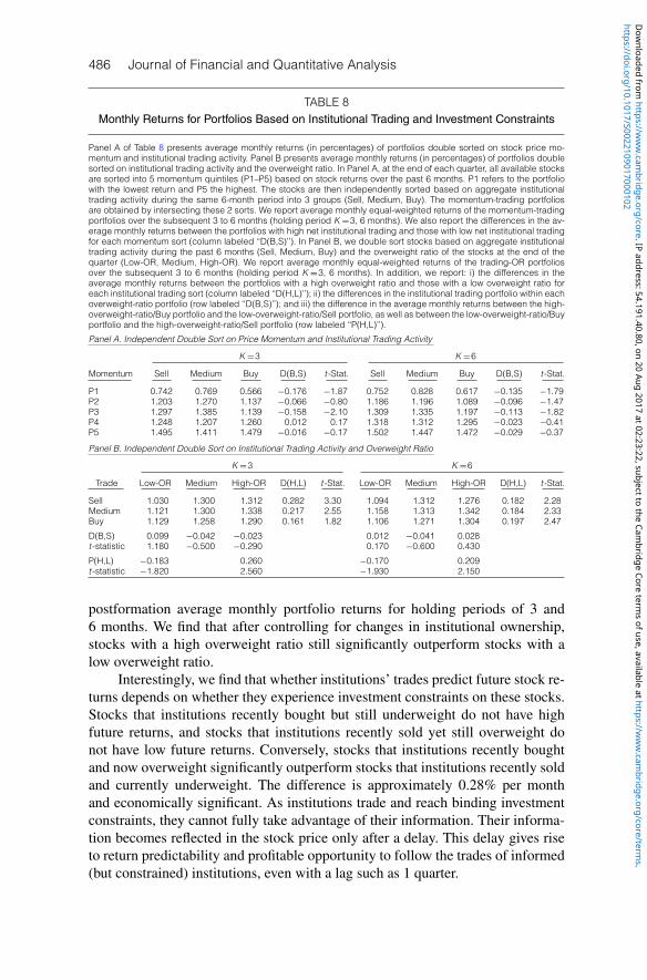
486 Journal of Financial and Quantitative Analysis
TABLE 8Monthly Returns for Portfolios Based on Institutional Trading and Investment Constraints
Panel A of Table 8 presents average monthly returns (in percentages) of portfolios double sorted on stock price mo-mentum and institutional trading activity. Panel B presents average monthly returns (in percentages) of portfolios doublesorted on institutional trading activity and the overweight ratio. In Panel A, at the end of each quarter, all available stocksare sorted into 5 momentum quintiles (P1–P5) based on stock returns over the past 6 months. P1 refers to the portfoliowith the lowest return and P5 the highest. The stocks are then independently sorted based on aggregate institutionaltrading activity during the same 6-month period into 3 groups (Sell, Medium, Buy). The momentum-trading portfoliosare obtained by intersecting these 2 sorts. We report average monthly equal-weighted returns of the momentum-tradingportfolios over the subsequent 3 to 6 months (holding period K =3, 6 months). We also report the differences in the av-erage monthly returns between the portfolios with high net institutional trading and those with low net institutional tradingfor each momentum sort (column labeled ‘‘D(B,S)’’). In Panel B, we double sort stocks based on aggregate institutionaltrading activity during the past 6 months (Sell, Medium, Buy) and the overweight ratio of the stocks at the end of thequarter (Low-OR, Medium, High-OR). We report average monthly equal-weighted returns of the trading-OR portfoliosover the subsequent 3 to 6 months (holding period K =3, 6 months). In addition, we report: i) the differences in theaverage monthly returns between the portfolios with a high overweight ratio and those with a low overweight ratio foreach institutional trading sort (column labeled ‘‘D(H,L)’’); ii) the differences in the institutional trading portfolio within eachoverweight-ratio portfolio (row labeled ‘‘D(B,S)’’); and iii) the difference in the average monthly returns between the high-overweight-ratio/Buy portfolio and the low-overweight-ratio/Sell portfolio, as well as between the low-overweight-ratio/Buyportfolio and the high-overweight-ratio/Sell portfolio (row labeled ‘‘P(H,L)’’).
Panel A. Independent Double Sort on Price Momentum and Institutional Trading Activity
K =3 K =6
Momentum Sell Medium Buy D(B,S) t -Stat. Sell Medium Buy D(B,S) t -Stat.
P1 0.742 0.769 0.566 −0.176 −1.87 0.752 0.828 0.617 −0.135 −1.79P2 1.203 1.270 1.137 −0.066 −0.80 1.186 1.196 1.089 −0.096 −1.47P3 1.297 1.385 1.139 −0.158 −2.10 1.309 1.335 1.197 −0.113 −1.82P4 1.248 1.207 1.260 0.012 0.17 1.318 1.312 1.295 −0.023 −0.41P5 1.495 1.411 1.479 −0.016 −0.17 1.502 1.447 1.472 −0.029 −0.37
Panel B. Independent Double Sort on Institutional Trading Activity and Overweight Ratio
K =3 K =6
Trade Low-OR Medium High-OR D(H,L) t -Stat. Low-OR Medium High-OR D(H,L) t -Stat.
Sell 1.030 1.300 1.312 0.282 3.30 1.094 1.312 1.276 0.182 2.28Medium 1.121 1.300 1.338 0.217 2.55 1.158 1.313 1.342 0.184 2.33Buy 1.129 1.258 1.290 0.161 1.82 1.106 1.271 1.304 0.197 2.47
D(B,S) 0.099 −0.042 −0.023 0.012 −0.041 0.028t -statistic 1.180 −0.500 −0.290 0.170 −0.600 0.430
P(H,L) −0.183 0.260 −0.170 0.209t -statistic −1.820 2.560 −1.930 2.150
postformation average monthly portfolio returns for holding periods of 3 and6 months. We find that after controlling for changes in institutional ownership,stocks with a high overweight ratio still significantly outperform stocks with alow overweight ratio.
Interestingly, we find that whether institutions’ trades predict future stock re-turns depends on whether they experience investment constraints on these stocks.Stocks that institutions recently bought but still underweight do not have highfuture returns, and stocks that institutions recently sold yet still overweight donot have low future returns. Conversely, stocks that institutions recently boughtand now overweight significantly outperform stocks that institutions recently soldand currently underweight. The difference is approximately 0.28% per monthand economically significant. As institutions trade and reach binding investmentconstraints, they cannot fully take advantage of their information. Their informa-tion becomes reflected in the stock price only after a delay. This delay gives riseto return predictability and profitable opportunity to follow the trades of informed(but constrained) institutions, even with a lag such as 1 quarter.
https://doi.org/10.1017/S0022109017000102D
ownloaded from
https://ww
w.cam
bridge.org/core . IP address: 54.191.40.80 , on 20 Aug 2017 at 02:23:22 , subject to the Cambridge Core term
s of use, available at https://ww
w.cam
bridge.org/core/terms .

Cao, Han, and Wang 487
V. ConclusionsInstitutional investors face constraints because of their restrictive investment
policies, which are not binding on individuals. These additional restrictions are amitigation of the legal liability imposed on institutional fiduciaries by laws andregulations such as ERISA and the Prudent Investor Rule.
This study examines the impact of institutional investment constraints onthe aggregate demand for stocks and the cross section of stock returns. Usinginstitutional equity holding data between 1980 and 2013, we find that institutionalinvestors are less likely to buy more of the stocks that they already overweighteven when there is good news about the stocks. They are also reluctant to sellthe stocks that they already underweight even when they have bad news about thestocks. This behavior is consistent with institutional investment constraints suchas diversification requirements and tracking-error restrictions.
We test hypotheses about the impact of institutional investment constraintson stock prices: Stocks that institutions overweight may underreact to good newsand become undervalued; stocks that institutions underweight may underreact tobad news and become overvalued. Consistent with the hypotheses, we find thatamong stocks that have good news, those that institutions overweight significantlysubsequently outperform those that institutions underweight. Similarly, for stocksthat have bad news, those that institutions underweight subsequently underper-form those that institutions overweight. Further, we find that the momentum strat-egy and post–earnings announcement drift are both stronger among stocks thatexperience high institutional investment constraints.
Our results support the argument of Allen (2001) that financial institutionsmatter for asset pricing. They indicate that asset pricing anomalies may be impor-tantly related to institutional investment constraints. In a similar vein, Alankar,Blaustein, and Scholes (2014) demonstrate that investment managers may noteliminate the observed asset pricing anomalies because they may contribute totheir existence. DeVault, Sias, and Starks (2014) argue that institutional investorsare the sentiment traders whose demand shocks drive prices from fundamentalvalue. Edelen, Ince, and Kadlec (2014) document that institutions are on thewrong side of anomalies more often than not. Goldman and Slezak (2003) showthat delegated portfolio management may distort managers’ incentive to tradeon long-term information and cause stock mispricing. It seems a fruitful venuefor future research to explore further how issues arising from delegated portfo-lio management affect money managers’ portfolio decisions and stock prices inequilibrium, following the lead of Roll (1992), Carpenter (2000), Cornell and Roll(2005), Cuoco and Kaniel (2011), and others.
ReferencesAlankar, A.; P. Blaustein; and M. Scholes. “The Cost of Constraints: Risk Management, Agency The-
ory and Asset Prices.” Working Paper, Stanford University (2014).Alexander, G.; G. Cici; and S. Gibson. “Does Trade Motivation Matter? An Analysis of Mutual Fund
Trades.” Review of Financial Studies, 20 (2007), 125–150.Allen, F. “Do Financial Institutions Matter?” Journal of Finance, 56 (2001), 1165–1175.Almazan, A.; K. C. Brown; M. Carlson; and D. A. Chapman. “Why Constrain Your Mutual Fund
Manager?” Journal of Financial Economics, 73 (2004), 289–321.
https://doi.org/10.1017/S0022109017000102D
ownloaded from
https://ww
w.cam
bridge.org/core . IP address: 54.191.40.80 , on 20 Aug 2017 at 02:23:22 , subject to the Cambridge Core term
s of use, available at https://ww
w.cam
bridge.org/core/terms .

488 Journal of Financial and Quantitative Analysis
Arnott, R. “What Risk Matters? A Call for Papers!” Financial Analysts Journal, 59 (2003), 6–8.Badrinath, S. G.; G. D. Gay; and J. R. Kale. “Patterns of Institutional Investment, Prudence, and the
Managerial ‘Safety-Net’ Hypothesis.” Journal of Risk and Insurance, 56 (1989), 605–629.Baker, M.; L. Litov; J. Wachter; and J. Wurgler. “Can Mutual Fund Managers Pick Stocks? Evidence
from the Trades Prior to Earnings Announcements.” Journal of Financial and QuantitativeAnalysis, 45 (2010), 1111–1131.
Barberis, N.; A. Shleifer; and R. Vishny. “A Model of Investor Sentiment.” Journal of FinancialEconomics, 49 (1998), 307–343.
Bennett, J.; R. Sias; and L. Starks. “Greener Pastures and the Impact of Dynamic InstitutionalPreferences.” Review of Financial Studies, 16 (2003), 1203–1239.
Bushee, B., and C. Noe. “Corporate Disclosure Practices, Institutional Investors, and Stock ReturnVolatility.” Journal of Accounting Research, 38 (2000), 171–202.
Cai, F., and L. Zheng. “Institutional Trading and Stock Returns.” Finance Research Letters, 1 (2004),178–189.
Carpenter, J. “The Optimal Dynamic Investment Policy for a Fund Manager Compensated with anIncentive Fee.” Journal of Finance, 55 (2000), 2311–2331.
Chan, L. K. C.; H. Chen; and J. Lakonishok. “On Mutual Fund Investment Styles.” Review of FinancialStudies, 15 (2002), 1407–1437.
Cohen, R.; P. Gompers; and T. Vuolteenaho. “Who Underreacts to Cash-Flow News? Evidencefrom Trading between Individuals and Institutions.” Journal of Financial Economics, 66 (2002),409–462.
Cohen, R. B.; C. K. Polk; and B. Silli. “Best Ideas.” Working Paper, Harvard University (2010).Cornell, B., and R. Roll. “A Delegated-Agent Asset-Pricing Model.” Financial Analysts Journal, 61
(2005), 57–69.Coval, J. D., and E. Stafford. “Asset Fire Sales (and Purchases) in Equity Markets.” Journal of
Financial Economics, 86 (2007), 479–512.Cremers, M., and A. Petajisto. “How Active Is Your Fund Manager? A New Measure That Predicts
Performance.” Review of Financial Studies, 22 (2009), 3329–3365.Cuoco, D., and R. Kaniel. “Equilibrium Prices in the Presence of Delegated Portfolio Management.”
Journal of Financial Economics, 101 (2011), 264–296.Daniel, K., and T. Moskowitz. “Momentum Crashes.” Swiss Finance Institute Research Paper No.
13-61; Columbia Business School Research Paper No. 14-6; Fama–Miller Working Paper (2013).Del Guercio, D. “The Distorting Effect of the Prudent-Man Laws on Institutional Equity Investments.”
Journal of Financial Economics, 40 (1996), 31–62.DeVault, L.; R. Sias; and L. Starks. “Who Are the Sentiment Traders? Evidence from the Cross-
Section of Stock Returns and Demand.” Working Paper, University of Arizona and University ofTexas (2014).
Edelen, R. M.; O. S. Ince; and G. B. Kadlec. “Institutional Investors and Stock Return Anomalies.”Working Paper, University of California at Davis and Virginia Tech (2014).
Edmans, A.; I. Goldstein; and W. Jiang. “The Real Effects of Financial Markets: The Impact of Priceson Takeovers.” Journal of Finance, 67 (2012), 933–971.
Falkenstein, E. “Preferences for Stock Characteristics as Revealed by Mutual Fund PortfolioHoldings.” Journal of Finance, 51 (1996), 111–136.
Fama, E., and K. French. “The Cross-Section of Expected Stock Returns.” Journal of Finance, 47(1992), 427–465.
Fama, E., and J. MacBeth. “Risk, Return and Equilibrium: Empirical Tests.” Journal of PoliticalEconomy, 81 (1973), 607–636.
Goldman, E., and S. Slezak. “Delegated Portfolio Management and Rational Prolonged Mispricing.”Journal of Finance, 58 (2003), 283–311.
Gompers, P., and A. Metrick. “Institutional Investors and Equity Prices.” Quarterly Journal ofEconomics, 116 (2001), 229–260.
Hirshleifer, D.; J. Myers; L. Myers; and S. H. Teoh. “Do Individual Investors Cause Post-EarningsAnnouncement Drift? Direct Evidence from Personal Trades.” Accounting Review, 83 (2008),1521–1550.
Hong, H., and J. C. Stein. “A Unified Theory of Underreaction, Momentum Trading and Overreactionin Asset Markets.” Journal of Finance, 54 (1999), 2143–2184.
Jegadeesh, N., and S. Titman. “Returns to Buying Winners and Selling Losers: Implications for StockMarket Efficiency.” Journal of Finance, 48 (1993), 65–91.
Jiang, H.; M. Verbeek; and Y. Wang. “Information Content When Mutual Funds Deviate fromBenchmarks.” Management Science, 60 (2014), 2038–2053.
Khan, M.; L. Kogan; and G. Serafeim. “Mutual Fund Trading Pressure: Firm-Level Stock Price Impactand Timing of SEOs.” Journal of Finance, 67 (2012), 1371–1395.
https://doi.org/10.1017/S0022109017000102D
ownloaded from
https://ww
w.cam
bridge.org/core . IP address: 54.191.40.80 , on 20 Aug 2017 at 02:23:22 , subject to the Cambridge Core term
s of use, available at https://ww
w.cam
bridge.org/core/terms .

Cao, Han, and Wang 489
Lakonishok, J.; A. Shleifer; and R. W. Vishny. “The Impact of Institutional Trading on Stock Prices.”Journal of Financial Economics, 32 (1992), 23–44.
Lakonishok, J.; A. Shleifer; and R. W. Vishny. “What Do Money Managers Do?” Working Paper,Harvard University (1997).
Lewellen, J. “Institutional Investors and the Limits of Arbitrage.” Journal of Financial Economics,102 (2011), 62–80.
Maug, E., and N. Naik. “Herding and Delegated Portfolio Management: The Impact of RelativePerformance Evaluation on Asset Allocation.” Quarterly Journal of Finance, 1 (2011), 265–292.
O’Barr, W. M., and J. M. Conley. Fortune and Folly: The Wealth and Power of Institutional Investing.Homewood, IL: Business One Irwin (1992).
Roll, R. “A Mean/Variance Analysis of Tracking Error.” Journal of Portfolio Management, 18 (1992),13–22.
Wermers, R.; T. Yao; and J. Zhao. “Forecasting Stock Returns through an Efficient Aggregation ofMutual Fund Holdings.” Review of Financial Studies, 25 (2012), 3490–3529.
https://doi.org/10.1017/S0022109017000102D
ownloaded from
https://ww
w.cam
bridge.org/core . IP address: 54.191.40.80 , on 20 Aug 2017 at 02:23:22 , subject to the Cambridge Core term
s of use, available at https://ww
w.cam
bridge.org/core/terms .