institute of aeronautical engineering (autonomous ... viii sem ln.pdf · aximization. ame021.08...
TRANSCRIPT

1
INSTITUTE OF AERONAUTICAL ENGINEERING (Autonomous)
Dundigal, Hyderabad -500 043
MECHANICAL ENGINEERING
COURSE LECTURE NOTES
Course Name OPERATIONS RESEARCH
Course Code AME021
Program B.Tech
Semester VIII
Year 2019-2020
Course Coordinator Mr. C. Labesh Kumar, Assistant Professor, ME
Course Faculty Ms. T vanaja, Assistant Professor
Lecture Numbers 1-63
Topic Covered All
COURSE OBJECTIVES
S.NO Description
I Formulate the mathematical model of real time problem for optimization.
II Establish the problem formulation by using linear, dynamic programming, game theory and queuing
models.
III Apply stochastic models for discrete and continuous variables to control inventory.
IV Visualize the computer based manufacturing simulation models.
COURSE OUTCOMES
S.NO Description
I Formulate the mathematical model of real time problem for optimization, using Linear programming
II Establish the problem formulation by using transportation, assignment models
III Apply sequencing for flow and replacement for maintenance of machinesprogramming, game
theory and queuing models.
IV Formulate game theory model and apply stochastic models for discrete and continuous variables to
control inventory.
V Formulate queuing models and visualize dynamic programming and simulation models
COURSE LEARNING OUTCOMES
Students, who complete the course, will have demonstrated the ability to do the following:
S. No. Outcomes
AME021.01 Understand the characteristics, phases, types of operation research models and its applications.
AME021.02 Visualize modeling principles scope, decision making, general methods for solving OR

2
models.
AME021.03 Understand linear programming concept problem formulation and graphical models.
AME021.04 Understand simplex method and artificial variable techniques.
AME021.05 Comprehend two-phase method and Big-M method of linear programming.
AME021.06 Apply to build and solve transportation models of balanced.
AME021.07 Understand the degeneracy model problem of transportation, unbalanced type-aximization.
AME021.08 Apply to build assignment models for optimal solution.
AME021.09 Understand variants of assignment model and travelling salesman model.
AME021.10 Understand the flow shop sequencing model of ‘n’ jobs through two machines and three
machines.
AME021.11 Comprehend job shop sequencing of two jobs through ‘m’ machines.
AME021.12 Understand the concept of replacement of items that deteriorate with time when money value is not counted
AME013.13 Understand the concept ofreplacement of items that deteriorate with time when money value is n counted .
AME021.14 Visualize the replacement of items that fail completely and group replacement.
AME021.15 Understand minmax (maximini) criterion, optimal strategy , solution od games with saddle point
AME021.16 Visualize dominance principle while solving game theory problem.
AME021.17 Apply to solve m * 2 , 2 *n model of games and graphical method.
AME021.18 Understand the concepts of deterministic inventory model and purchase inventory model with one price break and multiple price breaks.
AME021.19 Visualize stochastic inventory models – demand may be discrete variable or continuous variable.
AME021.20 Understand the concepts of waiting line model of single channel and multi server model.
AME021.21 Visualize dynamic programming concepts and models
AME021.22 Comprehend the simulation models, phases of simulation, application of simulation
AME021.23 Visualize the application of simulation for inventory and queuing problems.
UNIT-I
DEVELOPMENT OF OR AND ALLOCATION
Operations Research is the science of rational decision-making and the study, design and integration of
complex situations and systems with the goal of predicting system behavior and improving or
optimizing system performance.The formal activities of operation research were initiated in England
during World War II to make decisions regarding the best utilization of war material. After the war the
ideas advanced in military operations were adapted to improve efficiency and productivity in the
civilian sector. That developed to today’s dominant and indispensable decision-making tool,
Operations research. It encompasses managerial decision making, mathematical and computer
modeling and the use of information technology for informeddecision-making.

3
The concepts and methods of Operations Research are pervasive. Students and graduates advise the
public and private sectors on energy policy; design and operation of urban emergency systems; defense;
health care; water resource planning; the criminal justice system; transportation issues. They also
address a wide variety of design and operational issues in communication and data networks; computer
operations; marketing; finance; inventory planning; manufacturing; and many areas designed to
improve business productivity and efficiency. The subject impacts biology, the internet, the airline
system, international banking and finance. It is a subject of beauty, depth, infinite breadth
andapplicability.
The Meaning of Operations Research
From the historical and philosophical summary just presented, it should be apparent that the term
“operations research” has a number of quite distinct variations of meaning. To some, OR is that certain
body of problems, techniques, and solutions that has been accumulated under the name of OR over the
past 30 years, and we apply OR when we recognize a problem of that certain genre. To others, it is an
activity or process something we do, rather than know-which by its very nature isapplied.
Perhaps in time the meaning will stabilize, but at this point it would be premature to exclude any of
these interpretations. It would also be counterproductive to attempt to make distinctions between
“operations research” and the “systems approach.” While these terms are sometimes viewed as distinct,
they are often conceptualized in such a manner as to defy separation. Any attempt to draw boundaries
between them would in practice bearbitrary.
The Operational Research Society of Great Britain has adopted the following definition:
Operational research is the application of the methods of science to complex problems arising in
the direction and management of large systems of men, machines, materials and money in
industry, business, government, and defense. The distinctive approach is to develop a scientific
model of the system, incorporating measurements of factors such as chance and risk, with
which to predict and compare the outcomes of alternative decisions, strategies or controls. The
purpose is to help management determine its policy and actionsscientifically.
Operations research is concerned with scientifically deciding how to best design and operate

4
man- machine systems, usually under conditions requiring the allocation of scarce resources.
Although both of these definitions leave something to be desired, they are about as specific as
one would want to be in defining such a broad area. It is noteworthy that both definitions
emphasize the motivation for the work; namely, to aid decision makers in dealing with complex
real-world problems. Even when the methods seem to become so abstract as to lose real-world
relevance, the student may take some comfort in the fact that the ultimate goal is always some
useful application.
Both definitions also mention methodology, describing it only very generally as “scientific.”
That term is perhaps a bit too general, inasmuch as the methods of science are so diverse and
varied. A more precise description of the OR methodology would indicate its reliance on
“models.” Of course, that term would itself require further elaboration, and it is to that task that
we now turn ourattention.
Operations Research has been defined so far in various ways and still not been defined in an
authoritative way. Some important and interesting opinions about the definition of OR which
have been changed according to the development of the subject been givenbelow:
OR is a scientific method of providing executive departments with a quantitative basis for
decision regarding the operations under their control. -Morse andKimbal(9164)
OR is a scientific method of providing executive with an analytical and objective basis for
decisions. - P.M.S.Blacket(1948)
OR is the application of scientific methods, techniques and tools to problems involving the
operations of systems so as to provide these in control of the operations with optimum solutions
to theproblem.” - Churchman, Acoff, Arnoff (1957)
OR is the art of giving bad answers to problems to which otherwise worse answers are given.-
T. L Saaty (1958)
CHARECTERISTIS (FEATURES) OPERATIONS RESEARCH
The main characteristics of OR are as follows:
1) Inter-disciplinary team approach: In OR, the optimum solution is foud by a team of scientists

5
selected from various disciplines such as mathematics, statistics, economics, engineering,
physics, etc.
2) Wholistic approach to the system: The most of the problems tackled by OR have the
characteristic that OR have the characteristic that OR tries to find the best (optimum) deisions
relative to larger possible portion of the total organization.
3) Imperfectness of solutions: by OR techniques, we cannot obtain perfect answers to our
problems but, only the quality of the solution is improved from worse to bad answers.
4) Use of scientific research: OR uses techniques of scientific research to reach the optimum
solutions.
5) To optimize the total output> OR tries to optimize total return by maximizing the profit and
minimizing the cost or loss.
APPLICATIONS OF OPEARATIONS RESEARCH
1) In Agriculture:
-Optimum allocation of land to various crops in accordance with climatic conditions.
- Optimum distribution of water from various resources like canal for irrigation purposes.
2) In Finance:
-To maximize the per capita income with minimum recourses.
-To find out the profit plan for the company.
-To determine the best replacement policies.
3) In Industry:allocation of various limited resources such as men, machines, material, money,
4) In marketing:with th help of OR techniques a marketing manager can decide
Where to distribute the products for sles so that the total cost of transportation is minimum.
The minimum per unit cost sale price.
Thee size of stock to meet the future demand.
How to select the best advertising media with respect to time, cost etc.
How, when , and where to purchase at the minimum possible cost?
5) In Personnel Management: A Personnel manager can use OR techniques
To appoint the most suitable persons on minimum salary.
To determine the best age of retirement for employees.

6
To find out the number of persons to be appointed on full time basis when the work load is seasonal.
7) In Productionmanagement. A production manager can use OR techniques
To find out the number and size of the items to be replaced.
In scheduling and sequencing the production runs by proper allocation of machines.
In calculating the optimum product mix.
To select , locate and design the sites for production plants.
8) In LIC:
What should be the premium rates for various modes of policies.
How best the profits could be distributed in he case of with profit policies.
QUANTITATIVE TECHNIQUES OF OR:
Distribution (Allocation) Models: Distributionmodels are concerned with allotment of available
recourses so as to minimize cost or maximize profits subject to prescribed conditions.
Production/Inventory Models: These models are concerned with determination of the optimal
(economic) order quantity and ordering (production ) intervals considering the factors such s demand
per unit ime, cost of placing orders, costs associated with goods held up in he inventory and the cost
due to shortage of goods etc.
Waiting Line (Queueing) Models: In queueing models an attempt is made to predict
Markovian Models: These models are applicable in such a situations where the state of the system can
be defined by some descriptive measure of numerical value and here the system moves from one state
to another on a probability basis. Example is Brand switching problems
Competitive Strategy Models(Game Theory):These models are used to determine the ehaviour of
decission making under competition or conflict.
Network Models: These models are applicable in large projects involving complexities and inter-
dependencies od activities. PERT and CPM are used for planning , scheduling and controlling complex
project which can be characterized as net-work.
Job Sequencing Models: These models involve the selection of such a sequence of performing a
series of jobs to be done on service facilities(machines) that optimize th efficiency measure of
performance of the system.
Replacement Models: These models deal with determination of optimum replacement policy in

7
situation that arise when some items or machinery need replacement by a new one.
Simulation Models: Simulation is very powerful technique for solving such complex models which
cannot be solved otherwise and thus it is being extensively applied to solve a variety of problems.
MODELLING IN OPERATIONS RESEARCH
The essence of the operations research activity lies in the construction and use of models. Although
modeling must be learned from individual experimentation, we will attempt here to discuss it in broad,
almost philosophical terms. This overview is worth having, and setting a proper orientation in advance
may help to avoid misconceptionslater.
Definition: A model in the sense used in 0 R is defined as a representation of an actual object or
situation. It shows the relationships (direct or indirect) and inter-relationships of action and reaction in
terms of cause andeffect.
Since a model is an abstraction of reality, it thus appears to be less complete than reality itself. For a
model to be complete, it must be a representative of those aspects of reality that are being investigated.
The main objective of a model is to provide means for analyzing the behavior of the system for the
purpose of improving its performance. Or, if a system is not in existence, then a model defines the ideal
structure of this future system indicating the functional relationships among its elements. The reliability
of the solution obtained from a model depends on the validity of the model in representing the real
systems. A model permits to ‘examine the behavior of a system without interfering with
ongoingoperations.
CLASSIFICATION OF MODELS
Models can be Classified According to Following Characteristics:
Classification by Structure:
i. Iconic models. Iconic models represent the system as it is by scaling it up or down (i.e.,by enlarging or
reducing the size). In other words, it is an image.
For example, a toy airplane is an iconic model of a real one. Other common examples of it are:
photographs, drawings, maps etc. A model of an atom is scaled up so as to make it visible to the naked
eye. In a globe, the diameter of the earth is scaled down, but the globe has approximately the same

8
shape as the earth, and the relative sizes of continents, seas, etc., are approximately correct. The iconic
model is usually the simplest to conceive and the most specific and concrete. Its function is generally
descriptive rather than explanatory. Accordingly, it cannot be easily used to determine or predict what
effects many important changes on the actualsystem.
ii. Analogue models. The models, in which one set of properties is used to represent another set of
properties, are called analogue models. After the problem is solved, the solution is reinterpreted in
terms of the originalsystem.
For example, graphs are very simple analogues because distance is used to represent the properties such
as: time, number, percent, age, weight, and many other properties. Contour lines on a map represent the
rise and fall of the heights. In general, analogues are less specific, less concrete but easier to manipulate
than are iconic models.
iii. Symbolic (Mathematical) models. The symbolic or mathematical model is one which employs a
set of mathematical symbols (i.e., letters, numbers, etc.) to represent the decision variables of the
system. These variables are related together by means of a mathematical equation or a set of equations
to describe the behavior (or properties) of the system. The solution of the problem is then obtained by
applying well-developed mathematical techniques to the model. The symbolic model is usually the
easiest to manipulate experimentally and it is most general and abstract. Its function is more often
explanatory rather thandescriptive.
2. Classification by Purpose:
Models can also be classified by purpose of its utility. The purpose of a model may be descriptive
predictive or prescriptive.
i. Descriptive models. A descriptive model simply describes some aspects of a situation based on
observations, survey. Questionnaire results or other available data. The result of an opinion poll
represents a descriptivemodel.
Predictive models. Such models can answer ‘what if’ type of questions, i.e. they can make predictions
regarding certain events. For example, based on the survey results, television networks such models
attempt to explain and predict the election results before all the votes are actuallycounted.

9
ii. Prescriptive models. Finally, when a predictive model has been repeatedly successful, it can be used
to prescribe a source of action. For example, linear programming is a prescriptive (or normative) model
because it prescribes what the managers ought todo.
3. Classification by Nature ofEnvironment
These are mainly of two types:
i. Deterministic models. Such models assume conditions of complete certainty and perfect knowledge.
For example, linear programming, transportation and assignment models are deterministic type of
models.
Probabilistic (or Stochastic) models. These types of models usually handle such situations in which
the consequences or payoff of managerial actions cannot be predicted with certainty. However, it is
possible to forecast a pattern of events, based on which managerial decisions can be made. For
example, insurance companies are willing to insure against risk of fire, accidents, sickness and so on,
because the pattern of events have been compiled in the form of probability distributions.
4. Classification by Behavior
i. Static models. These models do not consider the impact of changes that takes place during the
planning horizon, i.e. they are independent of time. Also, in astatic model only one decision is needed
for the duration of a given timeperiod.
ii. Dynamic models. In these models, time is considered as one of the important variables and admits
the impact of changes generated by time. Also, in dynamic models, not only one but a series of
interdependent’ decisions is required during the planninghorizon.
5. Classification by Method ofSolution
i.Analytical models. These models have a specific mathematical structure-and thus can be solved by
known analytical or mathematical techniques. For example, general linear programming models as well
as the specially structured transportation and assignment models are analytical models. .
ii.Simulation models. They also have a mathematical structure but they cannot be solved by purely
using the ‘tools’ and ‘techniques’ of mathematics. A simulation model isessentiallycomputer-assisted

10
experimentation on a mathematical structure of a real time structure in order to study the system under
a variety of assumptions.
Simulation modeling has the advantage of being more flexible than mathematical modeling and hence
can be used to represent complex systems which otherwise cannot be formulated mathematically. On
the other hand, simulation has the disadvantage of not providing general solutions like those obtained
from successful mathematical models.
6. Classification by use of Digital Computers: The development of the digital computer has led to the
introduction of the following types of modeling in OR.
i. Analogue and Mathematical models combined. Sometimes analogue models are also expressed
interms of mathematical symbols. Such models may be long to both the types(ii)and(iii) in
classification 1 above.
For example, Simulation model is of analogue type but mathematical formulae are also used in it.
Managers very frequently use this model to ‘simulate’ their decisions by summarizing the activities of
industry in a scale-down period.
i. Function models. Such models are grouped on the basis of the function being performed.
For example, a function may serve to acquaint to scientist with such things as-tables, carrying data, a
blue-print of layouts, a program representing a sequence of operations (like’ in computer
programming).
iiQuantitative models. Such models are used to measure the observations.
For example, degree of temperature, yardstick, a unit of measurement of length value, etc.
Other examples of quantitative models are: (i) transformation models which are useful in converting a
measurement of one scale to another (e.g., Centigrade vs. Fahrenheit conversion scale), and (ii) the test
models that act as ‘standards’ against which measurements are compared (e.g., business dealings, a
specified standard production control, the quality of a medicine).
iii.Heuristic models:. These models are mainly used to explore alternative strategies (courses of
action) that were overlooked previously, whereas mathematical models are used to represent systems
possessing well- defined strategies. Heuristic models do not claim to find the best solution to
theproblem.

11
PRINCIPLES OF MODELING
Let us now outline general principles useful in guiding to formulate the models within the context of 0
R. The model building and their users both should be consciously aware of the following tenprinciples:
1. Do not build up a complicated model when simple one will suffice. Building the strongest possible
model is a common guiding principle for mathematicians who are attempting to extend the theory or to
develop techniques that have wide applications. However, in the actual practice of building models for
specific purposes, the best advice is to “keep itsimple”.
2. Beware of molding the problem to fit the technique. For example, an expert on linear programming
techniques may tend to view every problem he encounters as required in a linear programming
solutions. In fact, not all optimization problems involve only linear functions. Also, not all OR
problems involve optimization. As a matter of fact, not all real-world problems call for operations
research! Of course, everyone search reality in his own terms, so the field of OR is not unique in this
regard. Being human we rely on the methods we are most comfortable in using and have been most
successful within the past. We are certainly not able to use techniques in which we have no
competence, and we cannot hope to be competent in all techniques. We must divide OR experts into
three maincategories:
(i)Technique developers. (ii) Teacher and (iii) Problem solvers.
In particular one should be ready to tolerate the behavior “I have found a cure but I am trying to search
a disease to fit it” among technique developers and teachers.
3. The deduction phase of modeling must be conducted rigorously. The reason for requiring rigorous
deduction is that one wants to be sure that if model conclusions are inconsistent with reality, then the
defect lie in the assumptions. One application of this principle is that one must be extremely careful
when programming computers. Hidden “bugs” are especially dangerous when they do not prevent the
program from running but simply produce results, which are not consistent with the intention of the
model.
4. Models should be validated prior to implementation. For example, if a model is constructed to
forecast the monthly sales of a particular commodity, it could be tested using historical data to compare

12
the forecasts it would have produced to the actual sales. In case, if the model cannot be validated prior
to its implementation, then it can be implemented in phases for validation. For example a new model
for inventory control may be implemented for a certain selected
group of items while the older system is retained for the majority of remaining items. If the model
proves successful, more items can be placed within its range. It is also worth noting that real things
change in time. A highly satisfactory model may very well degrade with age. So periodic re-evaluation
is necessary.
5.A model should never be taken too literally. For example, suppose that one has to construct an
elaborate computer model of Indian economy with many competent researchers spending a great deal
of time and money in getting all kinds of complicated interactions and relationships. Under such
circumstances, it can be easily believed as if the model duplicates itself the real system. This danger
continues to increase as the models become larger and more sophisticated, as they must deal with
increasingly complicated problems.
6.A model should neither be pressed to do, nor criticized for failing to do that for which it was
never intended. One example of this error would be the use of forecasting model to predict so far into
the future that the data on which the forecasts are based have no relevance. Another example is the use
of certain network methods to describe the activities involved in a complex project. A model should not
be stretched beyond its capabilities.
7. Beware of over-selling a model. This principle is of particular importance for the OR professional
because most non- technical benefactors of an operations researcher’s work are not likely to understand
his methods. The increased technicality of one’s methods also increases the burden of responsibility on
the OR professional to distinguish clearly between his role as model manipulator and model interpreter.
In those cases where the assumptions can be challenged, it would be dishonest to use the model.
8. Some of the primary benefits of modeling are associated with the process of developing the
model. It is true in general that a model is never as useful to anyone else as it is to those who are
involved in building it up. The model itself never contains the full knowledge and understanding of the
real system that the builder must acquire in order to
Successfully model it, and there is no practical way to convey this knowledge and understanding

13
properly. In some cases the sole benefits may occur while the model is being developed. In such cases,
the model may have no further value once it is completed, An example of this case might occur when a
small group of people attempts to develop a formal plan for some subject. The plan is the final model,
but the real problem may be to agree on ‘what the objectives ought to be’.
9.A model cannot be any better than the information that goes into it. Like a computer program, a
model can only manipulate the data provided to it; it cannot recognize and correct for deficiencies in
input. Models may condense data or convert it to more useful forms, but they do not have the capacity
to generate it. In some situations it is always better to gather more information about the system instead
of exerting more efforts on modern constructions.
10.Models cannot replace decision makers. The purpose of OR models should not be supposed to
provide “Optimal solutions” free from human subjectivity and error. OR models can aid decision
makers and thereby permit better decisions to be made. However they do not make the job of decision
making easier. Definitely, the role of experience, intuition and judgment in decision- making is
undiminished.
GENERAL METHODS FOR SOLVING ‘OR’ MODLES
In OR, we do not have a single general technique that solves all mathematical models that arise in
practice. Instead, the type and complexity of the mathematical model dictate the nature of the solution
method. For example, in Section 1.1 the solution of the tickets problem requires simple ranking of the
alternatives based on the total purchasing price, whereas the solution of the rectangle problem utilizes
differential calculus to determine the maximum area.
The most prominent OR technique is linear programming. It is designed for models with strict linear
objective and constraint functions. Other techniques include integer programming (in which the
variables assume integer values), dynamic programming (in which the original model can be
decomposed into smaller sub. problems), network programming (in which the problem can be modeled
as a network), and nonlinear programming (in which the functions of the model are non. linear). The
cited techniques are but a partial list of the large number of available OR tools.
A peculiarity of most OR techniques is that solutions are not generally obtained in (formula-like)
closed forms. Instead, they are determined by algorithms. An algorithm provides fixed computational

14
rules that are applied repetitively to the problem with each repetition (called iteration) moving the
solution closer to the optimum. Because the computations associated with each iteration are typically
tedious and voluminous, it is imperative that these algorithms be executed on the computer. .
Some mathematical models may be so complex that it is impossible to solve them by any of the
available optimization algorithms. In such cases, it may be necessary to abandon the search for the
optimal solution and simply seek a good solution using heuristics or rules of thumb.
Generally three types of methods are used for solving OR models.
Analytic Method: If the OR model is solved by using all the tools of classical mathematics such as:
differential calculus and finite differences available for this task, then such type of solutions are called
analytic solutions. Solutions of various inventory models are obtained by adopting the so-called
analytic procedure.
Iterative Method: If classical methods fail because of complex- ity of the constraints or of the number
of variables, then we are usually forced to adopt an iterative method. Such a procedure starts with a
trial solution and a set of rules for improving it. The trial solution is then replaced by the improved
solution, and the process is repeated until either no further improvement is possible or the cost of
further calculation cannot be justified.
Iterative method can be divided into three groups:
a).After a finite number of repetitions, no further improvement will be possible.
b) Although successive iterations improve the solutions, we are only guaranteed the solution as a limit of
an infinite process.
c) Finally we include the trial and error method, which, however, is likely to be lengthy, tedious, and
costly even if electronic computers are used.
The Monte-Carlo Method: The basis of so-called Monte- Carlo technique is random sampling of
variable’s values from a Distribution of that variable. Monte-Carlo refers to the use of sampling
methods to estimate the value of non-stochastic variables
Steps of Monte-Carlo method:.

15
The following are the main steps of Monte-Carlo method:
Step 1. In order to have a general idea of the system, we first draw a flow diagram of the system.
Step 2. Then we take correct sample observations to select some suitable model for the system. In this
step we compute the probability distributions for the variables of our interest.
Step 3. We, then, convert the probability distributions to a cumulative distribution function. Step 4. A
sequence of random numbers is now selected with thehelp of random number tables.
Step 5. Next we determine the sequence of values of variables of interest with the sequence of random
numbers obtained instep 4.
Step 6. Finally we construct some standard mathematical function to the values obtained in step 5.Step
3. Step 4.Step
“Operations Research (Management Science) is a scientific approach to decision making that seeks to
best design and operate a system, usually under conditions requiring the allocation of scarce resources.”
A system is an organization of interdependent components that work together to accomplish the goal of
the system.
THE METHODOLOGY OF OR
When OR is used to solve a problem of an organization, the following seven step procedure should be
followed:
Step 1. Formulate the Problem
OR analyst first defines the organization's problem. Defining the problem includes specifying the
organization's objectives and the parts of the organization (or system) that must be studied before the
problem can be solved.
Step 2. Observe the System
Next, the analyst collects data to estimate the values of parameters that affect the organization's
problem. These estimates are used to develop (in Step 3) and evaluate (in Step4 a mathematical model
of the organization's problem. Step 3. Formulate a Mathematical Model of theProblem
The analyst, then, develops a mathematical model (in other words an idealized representation) of the
16
problem. In this class, we describe many mathematical techniques that can be used to model systems.
Step 4. Verify the Model and Use the Model for Prediction
The analyst now tries to determine if the mathematical model developed in Step 3 is an accurate
representation of reality. To determine how well the model fits reality, one determines how valid the
model is for the current situation.
Step 5. Select a Suitable Alternative
Given a model and a set of alternatives, the analyst chooses the alternative (if there is one) that best
meets the organization's objectives.
Sometimes the set of alternatives is subject to certain restrictions and constraints. In many situations,
the best alternative may be impossible or too costly to determine.
Step 6. Present the Results and Conclusions of the Study
In this step, the analyst presents the model and the recommendations from Step 5 to the decision
making individual or group. In some situations, one might present several alternatives and let the
organization choose the decision maker(s) choose the one that best meets her/his/their needs.After
presenting the results of the OR study to the decision maker(s), the analyst may find that s/he does not
(or they do not) approve of the recommendations. This may result from incorrect definition of the
problem on hand or from failure to involve decision maker(s) from the start of the project. In this case,
the analyst should return to Step 1, 2,or3.
Step 7. Implement and Evaluate Recommendation
If the decision maker(s) has accepted the study, the analyst aids in implementing the recommendations.
The system must be constantly monitored (and updated dynamically as the environment changes) to
ensure that the recommendations are enabling decision maker(s) to meet her/his/theirobjectives.
LINEARPROGRAMMING Introduction Observe the world and predictable patterns will emerge. When air pressure falls, bad weather often
follows. High and low tides relate to the setting and rising of the moon. Hair and eye color pass from
parent to child. Patterns emerge from systems as small as the atom and as large as the universe.

17
Mathematics allows us to express these patterns as equations, and thereby to predict future changes.
Linear algebra, the mathematics of systems of equations, further allows complex interactions within a
system to be expressed as a unified entity representing the entire system all at once: amatrix.
Linear algebra provides the methods necessary to analyze unwieldy systems. Insight into information
such as the stresses and strains at multiple locations in a building, harmonic frequencies of an aircraft
design, and how to maximize and minimize many individual aspects of an entire system allows the
development of larger and more complex designs. Of special interest to industry, even after 40 years
of intense research, is the ability to optimize.
Linear Programming:Linear programming is a powerful quantitative technique (or operational
research technique) designs to solve allocation problem. The term ‘linear programming’ consists
of the two words ‘Linear’ and ‘Programming’. The word ‘Linear’ is used to describe the relationship
between decision variables, which are directly proportional. For example, if doubling (or tripling) the
production of a product will exactly double (or triple) the profit and required resources, then it is linear
relationship. The word ‘programming’ means planning of activities in a manner thatachieves some
‘optimal’ result with available resources. A programme is ‘optimal’ if it maximizes or minimizes
some measure or criterion of effectiveness such as profit, contribution (i.e. sales-variable cost), sales,
and cost. Thus, ‘Linear Program- ming’ indicates the planning of decision variables, which are directly
proportional, to achieve the ‘optimal’ result considering the limitations within which the problem is to
besolved.
Decision Variables:
The decision variables refer to the economic or physical quantities, which are competing with one
another for sharing the given limited resources. The relationship among these variables must be linear
under linear programming. The numerical values of decision variables indicate the solution of the
linear programming problem
Objective Function
The objective function of a linear programming problem is a linear function of the decision variable

18
expressing the objective of the decision maker. For example, maximization of profit or contribution,
minimization of cost/time.
Constraints
The constraints indicate limitations on the resources, which are to be allocated among various decision
variables. These resources may be production capacity, manpower, time, space or machinery. These
must be capable of being expressed as linear equation (i.e. =) on inequalities (i.e. > or<; type) in terms
of decision variables. Thus, constraints of a linear programming problem are linear equalities or
inequalities arising out of practicallimitations.
Non-negativity Restriction
Non-negativity restriction indicates that all decision variables must take on values equal to or greater
than zero.
Divisibility
Divisibility means that the numerical values of the decision variables are continuous and not limited to
integers. In other words, fractional values of the decision variables must be permissible in obtaining
optimal solution.
FORMULATION OF LP PROBLEMS
Step Involved in the Formulation of LP Problem
The steps involved in the formation of linear programming problem are as follows:
Step 1: Identify the Decision Variables of interest to the decision maker and express them as X1, X2,
X3
Step 2: Ascertain the Objective of the decision maker whether he wants to minimize or to maximize.
Step 3: Ascertain the cost (in case of minimization problem) or the profit (in case of maximization
problem) per unit of each of the decision variables.
Step 4: Ascertain the constraints representing the maximum availability or minimum commitment or
equality and represent them as less than or equal to (≤ type inequality or greater than or equal to (>≥)
type inequality or ‘equal to’ (=) type equalityrespectively.
Step 5: Put non-negativity restriction as under: Xj> 0; j = 1, 2… n (non-negativity restriction) Step 6:

19
Now formulate the LP problem as under:
Example-1: (Production allocation problem): A firm manufactures two types of products A and B and
sells them at a profit of Rs. 2 on type A and Rs 3 on type B. Each product is processed on two
machines G and H. Type A requires one minute of processing time on G and two minutes on H; type
B requires one minute on G and one minute on H. the machine G is available for not more than 6 hour
40 minutes while machine H is available for 10 hours during any of working day. Formulate the
problem as a linear programming problem.
Formulation: let X1 be the number of products of type A
X2 the number products of type B.
After carefully understanding the problem, the given information can be systematically arranged in
the form of the following table:
Table-1
time of products
(minutes)
Available
time
(minutes)
TypeA (X1 units ) Type B (X2
units )
G 1 1 400
H 2 1 600
Profit per unit Rs 2 Rs 3
Since the profit on type A is Rs 2 per product, and Rs 3 on product B.
The total profit for X1 units of typew A, and X2 units of type B . Z = 2X1 + 3X2 (objective
function)
Considering processing time on machine G for processing X1 units of type A, and X2 units of type B
= 1 X1 + 1 X2
but machine G available time is –400 minutes
1 X1 + 1 X2≤400 ------ eqn-1 (first constraint)
Considering processing time on machine H for processing X1 units of type A, and X2 units of type B
= 2 X1 + 1 X2
but machine H available time is – 600 minutes
1 X1 + 1 X2≤ 600 ------ eqn-2 (second constraint)

20
Since it is not possible to produce negative quantities
X1 ≥ 0, X2 ≥ 0 (non negativity restrictions
Hence the allocation problem of the firm ca be finally put in the form
Example-2. A company produces two types of Hats. Each hat of first type requires twice as much
labour than the second type. If all the hats are of the second type only, the company can produce a
total of 500 hats a day. The material limits the daily sales of the first and second type to 150 and 250
hats . Assuming that the profits per hat are Rs8 for type A and Rs 5 for type B, formulate the problem
as a linear programming model in order to determine the number of hats of each type so as to
maximize the profit.
Formulation: let X1 be the numberof units of hat type A
X2 be the number of units of hat type B.
After carefully understanding the problem, the given information can be systematically arranged in
the form of the following table:
Table-1
Machine time of products (minutes) Available
time
(minutes)
Type A (X1
units )
Type B (X2
units )
hat type A 2t 1t 500 t
Hat Type B 2 1 600
Profit pper
unit
Rs 8 Rs 5
Since the profit on hat of type A is Rs 8 per unit, , and Rs 5 on hat of type B.
The total profit for X1 units of type A, and X2 units of type B . Z = 8X1 + 5X2 (objective
function)
Since the company can produce a at the most 500 hats in a day and a type of hat requires twice as
mach time as that of hat type B, the production restriction is given by 2*t X1 + 1*t X2 ≤500 t where t
Find X1 and X2 such that the profit Z = 2X1 + 3X2 is maximum
subject to the conditions:
1 X1 + 1 X2≤400 ,
1 X1 + 1 X2≤ 600
X1 ≥ 0, X2 ≥ 0

21
is the labour time per unit of second type ie
2X1 + X2 ≤500 ----- constraint-1
Considering limitations on the sale of hats
X1≤ 150
X2≤250
Also , since the company cannot produce negative quantities
X1 ≥ 0, X2 ≥ 0 (non negativity restrictions
Hence the allocation problem of the firm ca be finally put in the form
Example-3.. manufacturer of patent medicines is proposed to prepare a production plan for medicines
A and B. There are sufficient ingredients available to make 20,000 bottles of medicine A and 40,000
bottles of medicine B, but there are only 45,000 bottles into which either of the medicines canbe
filled. Further it takes three hours to prepare enough material to fill 1000 bottles of medicine A and 1
hour to prepare enough material to fill 1000 bottles of medicine B, and there are 66 hours available for
this application. The profit is Rs 8 per bottle for medicine A and Rs 7 per bottle for medicine
B.Further, it takes three hours to prepare enough material to fill1000 bottles of medicine A and one
hour to prepare enough material to fill 1 000 bottles of medicine B, and there are 66hours available for
this operation. The profit is Rs. 8 per bottle for medicine A and Rs. 7 per bottle for medicineB.
i. Formulate this problem as a LP.P.,
ii. How the manufacturer schedule his production in order to maximizeprofit.
Formulation.
(i) Suppose the manufacturer produces XI and X2 thousand of bottles of medicines A and B,
respectively. Since it takes three hours to prepare 1000 bottles of medicine A,
The time required to fill XI thousand bottles of medicine A will be 3X1 hours. Similarly, the time
required to prepare X2thousand bottles of medicine B will be X2 hours. Therefore, total time required
to prepare XI thousand bottles of medicine A and X2 thousand bottles of medicine B will be 3X1 + 1.
X2 .
Since the total time available for this operation is 66 hours,
The constraint becomes 3X1 + 1. X2 . ≤ 66
Find X1 and X2 such that the profit Z = 8X1 + 5X2 is maximum
subject to the restrictions:
2X1 + X2 ≤500
X1≤ 150
X2≤250 X1 ≥ 0, X2 ≥ 0

22
Since there are only 45 thousands bottles available for filling medicines A and B, the constraint
becomes X1 + X2 . ≤ 45
Considering ingredient availability, possible to make 20 thousands of medicine A and 40 thousands
bottles off medicine B, the constraints becomes
X1≤ 20
X2≤ 40
Number of bottles being non-negative, X1 ≥ 0, X2 ≥ 0
Considering profit: profit at the rate of Rs 8 per bottle for type A medicine and Rs 7 per bottle for type
B medicine,
The total profit on X1 thousands of medicine A and X2 thousands of medicine B will become
Profit Z =8*1000 X1 + 7 *1000X2 = 8000 X1 + 7000X2
Hence the allocation problem of the firm can be finally put in the form:
Example-4. Atoy company manufactures two types of doll, a basic version doll-A and a deluxe
version doll-B. each type of doll of type B takes twice as long to produce as one of type A, and the
company would have time to make a maximum of 2000 per day. The supply of plastic is sufficient to
produce 1500 dolls per day (both A and B combined). The deluxe version requires a fncy dress of
which there are only 600 per day available. If the company makes a profit of Rs 3 and Rs 5 per doll,
respectively on doll A and B, then how many of each doll should be produced per dy to maximize the
total profit. Formulate the problem.
Formulation: let X1 be the number of doll A.
X2 the number products of doll type B.
After carefully understanding the problem, the given information can be systematically arranged in
the form of the following table:
Find X1 and X2 such that the profit Z = 8000X1 + 7000X2 is
maximum
subject to the restrictions:
3X1 + 1. X2 . ≤ 66
X1 + X2 . ≤ 45
X1≤ 20
X2≤ 40
X1 ≥ 0, X2 ≥ 0

23
Machine Availabilit
y
Doll A (X1
units )
Type B (X2
units )
Time in hours t 2t 2000 t
Plastic material 2 1 1500
Dress constraint - 1 600
Profit pper unit Rs 3 Rs 5
Since the profit on doll A is Rs 3 per product, and Rs 5 on doll B.
The total profit for X1 units of doll A, and X2 units of doll B . Z = 3X1 + 5X2 (objective
function)
Considering processing time: let the doll A require t hours, so that the doll B require 2t hours. Since
the total time to manufacture X1 units of doll A, and X2 units of doll B . , should not exceed 2000t
hours. Therefore t X1 + 2 X2≤ 2000 t
Considering plastic material constant forX1 units of doll A, and X2 units of doll B
1 X1 + 1 X2≤ 1500 ------ eqn-2 (second constraint)
Considering fancy dress material constraint X2≤ 600
Since it is not possible to produce negative quantities of dolls
X1 ≥ 0, X2 ≥ 0 (non negativity restrictions
Hence the allocation problem of the firm can be finally put in the form
The solution can be found by graphical method also.
Example-4. A firm can produce three types of cloths, say A, B and C. three kinds of wool are required
for it, say: red, green and blue wool. One unit length of type A cloth needs 2 meters of red wool and 3
meters of blue wool; one unit length of type B cloth needs 3 meters of red wool, 2 meters of green
wool and 2 meters of blue wool; and one unit of typeC cloth needs 5 meters of green wool and 4
Find X1 and X2 such that the profit Z = 3X1 + 5X2 is maximum
subject to the conditions:
X1 + 2 X2≤ 2000,
X1 + 1X2 ≤ 1500
X2 ≤ 600 X1 ≥ 0, X2 ≥ 0

24
meters of blue wool. The firm has only a stock of 8 meters of red wool, 10 meters of green wool and
15 meters of blue wool. It is assumed that the income obtained from one unit length of type A cloth is
Rs 3.00, of type B cloth is Rs 5.00, and of type C cloth is Rs 4.00. Determine, how the firm should use
the available material so as to maximize the income from the finished cloth.
Formulation: after understanding the problem carefully it is convenient to represent the data in
following table.
let X1, X2, , X3,be quantity (in meters) produced of type A, B, C respectively.
Since the profit on type –A is Rs 3 per product, and Rs 5 on type-B, and Rs 4 on type-C.
The total profit for X1 units of type- A, and X2 units of type-B and X3 unitsof type-C .
Z = 3X1 + 5X2 +4X3 (objective function)
Since 2 meters of red wool are required for each meter of cloth A and 3 meters of this type of cloth
are required for each meter of cloth B and zero meter are required for each meter of cloth C.
Thus total quantity of red wool becomes: 2X1 + 3 X2 + 0 X3
Considering red wool availability of 8 meters, the constraint becomes
2X1 + 3 X2 + 0 X3 ≤8 --------- eqn-1
Considering green wool availability the constraint becomes : 0. X1 + 2 X2 + 5 X3 ≤10 ----eqn-2
Considering blue wool availability the constraint becomes : 3. X1 + 2 X2 + 4 X3 ≤ 1 5 ----- eqn-3
Since it is not possible to produce negative quantities of product A, B and C
X1 ≥ 0, X2 ≥ 0X3 ≥ 0 (non negativity restrictions )
Hence the allocation problem of the firm ca be finally put in the form
Quality of
wool
Availability of wool (in meters)
A (X1 units
)
B (X2 units ) C ( X2 units) Availabilityo
f wool
Red 2 3 0 8
Green 0 2 5 10
Blue 3 2 4 15
Income per unit
length of cloth
Rs 3 Rs 5 4
Find X1 and X2 such that the profit Z = 3X1 + 5X2 is maximum
subject to the conditions:
2X1 + 3 X2 + 0 X3 ≤ 8
2 X2 + 5 X3 ≤ 10
3X1 + 2 X2 + 4 X3 ≤ 1 5
and X1 ≥ 0, X2 ≥ 0 , X3 ≥ 0

25
L P GRAPHICAL SOLUTION
Linear programming graphical Method :
Graphical Method is used for solving linear programming problems that involve only two variables.
Closed Half Plane
A linear inequality in two variables is known as a half plane. The corresponding equality or the line is
known as the boundary of the half plane. The half plane along with its boundary is called a closed half
plane. Thus, a closed half plane is a linear inequality in two variables, which include the value of the
variable for which equality is attained.
Feasible Solution
Any non-negative solution which satisfies all the constraints is known as a feasible solution of
theproblem.
Feasible Region
The collection of all feasible solutions is known as a feasible region.
Convex Set
A set (or region) is convex if only if for any two points on the set, the line segment joining those
points lies entirely in the set. Thus, the collection of feasible solutions in a linear program- ming
problem form a convex set. In other words, the feasible region of a linear programming problem is a
convex set.
Convex Polygon
A convex polygon is a convex set formed by the intersection of a finite number of closed half planes.
Extreme Points or Vertexes or Corner Points
The extreme points of a convex polygon are the points of intersection of the lines bounding the
feasible region. The value of the decision variables, which maximize or minimize the objective
function is located on one of the extreme points of the convex polygon. If the maximum or minimum
value of a linear function defined over a convex polygon exists, then it must be on one of the extreme

26
points.
Redundant Constraint
Redundant constraint is a constraint, which does not affect the feasible region.
Multiple Solutions
Multiple solutions of a linear programming problem are solutions each of which maximize or
minimize the objective function. Under graphical method, the existence of multiple solutions is
indicated by a situation under which the objective function line coincides with one of the half planes
generated by a constraint. In other words, where both the objective function line and one of constraint
lines have the sameslope.
Unbounded Solution
An unbounded solution of a linear programming problem is a solution whose objective function is
infinite. A linear program- ming problem is said to have unbounded solution if its solution can be
made infinitely large without violating any of the constraints in the problem. Since there is no real
applied problem, which has infinite returns, hence an unbounded solution always represents a
problem that has been incorrectlyformulated.
For example, in a maximization problem at least one of the constraints must be an equality’ or ‘less
than or equal to’ (<) type. If all of the constraints are ‘greater than or equal to’ (>) type, then there will
be no upper limit on the feasible region. Similarly for minimization problem, at least one of
constraints must be an ‘equality’ or ‘a greater than or equal to’ type (>) if a solution is to bebounded.
Under graphical method, the feasible solution region extends indefinitely.
Infeasible Problem
A linear programming problem is said to be infeasible if there is no solution that satisfies all the
constraints. It represents a state of inconsistency in the set of constraints.
Practical Steps Involved in Solving LPP By Graphical Method
Simple linear programming problems of two decision variables can be easily solved by graphical
method. The outlines of graphical procedure are as follows:
Step 1: Consider each inequality constraint as equation.
Step 2: plot each equation on he graph, as each will geometrically represent a straight line.
\step-3. Shade the feasible region. Every point on the line will satisfy the equation of the line. If the
inequality- constraint corresponding to that line is ‘<=’, then the region below the line lying

27
in the first quadrant (due to non-negativity of variables) is shaded. For the equality –constraint with ‘
>=’ sign, the region above he line in the first quadrant is shaded. The points lying in the
common region will satisfy all the constraints simultaneously. The common region thus obtained is
called the feasible region.
Step-4. Choose the convenient value of Z (say =0 ) and plot the objective function line.
Step-5. Pull the objective function line until the extreme points of the feasible region. In the
maximization case, this line will stop farthest from the origin and passing through at least one carner
of he feasible region. In the minimization case, , the line , this line will stop nearest to the origin and
passing through at least one corner of the feasible region.
Step-6. Read the coordinates of the extreme point (s) selected in step-5, and find the maximum or
minimum (as the case may be) value of Z.
Example-1. Find a geometrical interpretation and a solution as well for the following
problem.(Graphical method)
Maximize Z = 3X1 + 5X2 , subjective to restrictions:
X1 + 2X2 ≤ 2000, , X1 + X2 ≤ 1500, , X2 ≤ 600 and X1≥ 0, , X2≥ 0,
Graphical Solution.
Step-1. To graph the inequality constraints, consider two mutually perpendicular lines OX1 and OX2
as axix of coordinates. Since X1, X2 ≥ 0 we have to draw in first quadrant only.
To plot the X1 + 2X2 ≤ 2000, consider the equation X1 + 2X2 = 2000, for x1 = 0, X2 =
1000; X2 = 0, X1= 2000
Take appropriate scale and reprensent the points and draw the line of X1 + 2X2 = 2000, since
constraint is of ≤ type, consider region toward the origin I as feasible region.
Consuder second constraint X1 + X2 ≤ 1500, , fo
when X1 =0 , X2= 1500
when X2=0 X1=1500
Consider third constraint X2 ≤ 600 , X2 = 600 , when X1=0, X2= 600
Similarly plot the all the straight lines and consider common n region towards origin satisfying all the

28
all the constraints as feasible region.
Step-2. Find the feasible region or solution space by combining all constraints. A common shaded
area of OABCD is obtained which is feasible solution to the given LPP. Which satisfies all the
constraints?
Step-3. Find the coordinates of the corner points of feasible region O, A, B, C, D
Step-4. Locate the corner point of optimal solution either by calculating the value of Z for each corner
point o, A, B, C and D.
Point A (0, 1500) Z = 3x1 + 5x2 = 0+ 7500) = 7500
At point B (1000, 500), Z =(3*1000 + 5*500) = 5500 maximum
At point C (800,600), Z= ( 3*800 + 5*600) = 5400
At point D (0, 600), Z= ( 3 *0 + 5* 600) = 3000
At point O (0, 0) Z = (3*0 + 5*0 ) =0
In this problem, maximum value of Z is attained at the corner point B (1000, 500), which is poin of

29
intersection of lines
X1 + 2X2 = 2000, and X1 + X2 ≤ 1500,
Hence the required solution is X1 = 1000, X2= 500 and maximum value Z = Rs 5500
ANOTHER METHOD TO FIND OPTIMUM POINT:
To find the point or points in the feasible region . for some fixed value of Z, Z = 3X1 + 5X2 is a
straight line and any point on it gives the same value of Z
Considering Z=3000, 3X1 + 5X2 =3000 when x1 = 0, X2= 600
When x2=0 X1 = 1000
Represent the objective function line also on the feasible region graph. Move th objective function
straight line parallely such that it touches the extreme poit on the feasible region.. it touches point C,
where x1 = 1000, X2= 500, maximum objective function value =Zmax = 5500.
Example-2.
Solve by graphical method Max Z = X1 + X2 Subject to
X1 + 2X2 ≤ 2000, , X1 + X2 ≤ 1500, , X2 ≤ 600 and X1≥ 0, , X2≥ 0,
Considering First constraint as equation X1 + 2X2 = 2000,
When [ X1 = 0, X2 = 1000 ] and When X2 =0 , X1 =2000 ,
Considering the second constraint as equation , X1 + X2 = 1500
when [ X1 = 0, X2 = 1500 ] & { When X2 =0 , X1 =1500 ]
The feasible region is similar to earlier problem.
It is clear from figure that Z is maximum and it lies along the edge AB of the polygon of the feasible
solutions. This indicates that the values of X1, X2, which maximize Z are not unique., but any point on
the edge AB of OABCD polygon will give the optimum value of Z. the maximum value of Z is always
unique, but there will be an infinite number of feasible solutions which give unique value of ‘Z’. thus ,
two corners A and B as well as any other point on the line AB (segment) will give optimal solution of

30
this problem.
It should be noted that if a linear programming problem has mre than one optimum solution, there
exists alternative optimum solutions.. and one of the optimum solutions will be corresponding to corner
point B. ie X1= 1000, X2= 500 with max. profit Z = 1000+500= 1500
Figure-2
Example-3: Solve the following LP problem graphically.
Max Z = 8000 X1 + 7000X2, subject to
3 X1 + X2 ≤ 66, X1+ 2X2 ≤ 45, X1≤ 20, X2 ≤ 40
and X1≥ 0, , X2≥ 0
Solution: First plot the lines 3 X1 + X2 = 66, X1+ 2X2 = 45, X1= 20 and X2 = 40 and
shade the fusible region as shown in fig-3.
Draw a dotted line 8000 X1 + 7000X2= 0 for z-0 and continue to draw the lines till a point is
obtained which is farthest from the origin but passing through at least one of the corners of the

31
shaded (feasible) region.
The figure shows that this point P (10.5, 34.5) which is the intersection of lines
3 X1 + X2 = 66,
X1+ 2X2 = 45,
Hence , Z is maximum for X1= 10.5 and X2= 34.5
Max Z = 8000* 100.5 + 7000*34.5 = Rs 325000.
GRAPHICAL METHOD FOR MINIMIZATION PROBLEM:
Consider the problem
Example-4. Min Z = 1.5 X1 + 2.5 X2 subject to

32
X1 + 3X2 ≥ 3 X1+ X2 ≥ 2 and X1≥ 0, , X2≥ 0
Graphical Solution: The geometrical interpretation of the problem is given in fig-7. The minimum is
attained at the point of intersection A of the lines
X1 + 3X2 = 3 and X1+ X2 = , 2 .This is the unique point to give the minimum value of
Z. now , solving these two equations
X1=
1.5 ,X2 = 0.5 and min Z = 3.5
GRAPHICAL SOLUTION IN SPECIAL EXCEPTIONAL CASES
Example -7 .( Problem having unbounded solution)
Max Z= 3X1 + 2 X2 subject to X1 – X2 ≤, 1 , X1 + X2 ≥ 3, and X1≥ 0, , X2≥ 0
GraphicalSolution: the region of feasible solution is the shaded area as

33
shown in figure-7.
It is clear from the figure that the line representing the objective function can be moved far even
parallel to itself in the direction of increasing Z, and still have some points in the region of feasible
solutions.
Hence Z can be made arbitrarily large, and the problem has no finite maximum value of Z. such
problems are said to have unbounded solutions.Infinite profit in practical problems of LP can not be
expected. If LP problem has been formulated by committing some mistake, it may lead to an
unbounded solution.
Example-8 Max Z= -3X1 + 2 X2 subject to X1 ≤, 3 , X1 – X2 ≤, 0 and X1 , X2≥ 0

34
Graphical Solution: I previous example-7, it has been seen that the both the variables can be made
arbitrarily large as Z is increased. In this problem, an unbounded solution does not necessarily imply
that all the variables can be made arbitrarily large as Z approaches infinity. Here the variable X1
remains constant as shown in figure.

35
Example-9. (problem which is not completely normal)
Maximize Z= -X1 + 2 X2 subject to - X1 +X2 ≤, 1 , - X1 + 2X2 ≥ 4 and X1 , X2≥ 0
Graphical solution: the problem is solved graphically in fig.
Observing graph figure-11., the lne of objective function coincides with the edge of equation-1 of the
region of the feasible solutions. Thus every point ( X1, X2) lying on this edge (- X1 + 2X2 = 4), which
is going infinity on the right gives Z=4 and is thereforean optimal; solution.
Example-10. (Problem with inconsistent system of constraints)
Maximize Z= 3X1 - 2 X2 subject to X1 +X2 ≤, 1 , 2X1 + 2X2 ≥ 4 and X1 , X2≥ 0
Graphical solution: the problem is represented graphically in fig-12. The figure shows that there is no
point (X1, X2) which satisfies both the constraints simultaneously. Hence the problem has no solution
because the constraints are inconsistent.

36
Example-13. (Constraint can be consistent and yet thee may be no solution)
Maximize Z= X1 + X2 subject to X1 - X2 ≥ 0 , -3X1 + X2 ≥ 3, and X1 , X2≥ 0

37
Graphical solution: the figure shows that there is no region of feasible solutions in this case. Hence
there is no feasible solution. So the question of having optimal solution does not arise.
Example-12. (Problem in which constraints are equations rather than inequalities)
Maximize Z= 5X1 + 3X2 subject to 3 X1 + 5X2 =15, , 5X1 + 2X2 = 10 , and X1 , X2≥ 0
Graphical solution: fig-14 shows the graphical solution. Since there is only a single solution point A (
20/19, 45/19), thee is nothing to be maximized. Hence , a problem of this kind is of no importance.

38
Such problems can arise only when the number of equations in the constraints is at least equal to the
number of variables. If the solution is feasible,
it is optimal,
INTRODUCTION TO SIMPLEX METHOD
The Simplex Method isa systematic procedure for generating and testing candidate vertex
solutions to a linear program.” (Gill,Murray,andWright,p.337). It begins at an arbitrary corner of
the solution set. At each iteration, the Simplex Method selects the variable that will produce the

39
largest change towards the minimum (or maximum) solution. That variable replaces one of its
compatriots that is most severely restricting it, thus moving the Simplex Method to a different
corner of the solution set and closer to the final solution. In addition, the Simplex Method can
determine if no solution actuallyexists.
The Simplex Method solves a linear program of the form described in figure. Here, the
coefficients represent the respective weights, or costs, of the variables . The minimized statement
is similarly called the cost of the solution.Thecoefficients of the system of
equations are represented by, and any constant values in the system of equations are combined on
the right-hand side of the inequality in the variables
. Combined, these statements represent a linear program, to which we seek a solution of
minimum cost.
This linear program involves solution of the set of equations.
If no solution to the set of equations is yet known, slack variables, xn+1, xn+2,……,Xn+m, adding no cost to
the solution are introduced. The initial basic feasible solution (BSF) will be the solution of the linear
program.
THE SIMPLEX METHOD DEFINITIONS
Objective Function: The function that is either being minimized or maximized. For example, it
may represent the cost that you are trying tominimize.
Optimal Solution: A vector x, which is both feasible (satisfying the constraints) and optimal
(obtaining the largest or smallest objectivevalue).
Constraints: A set of equalities and inequalities that the feasible solution must satisfy.
Feasible Solution: A solution vector, x, which satisfies the constraints.
Basic Solution: x of (Ax=b) is a basic solution if the n components of x can be partitioned in to m
“basic” and n-m“ non-basic” variables in such a way that: them columns of A corresponding to the

40
basic variables forma nonsingular basis and the value of each “non-basic” variable is0.
The constraint matrix A has m rows (constraints) and n columns (variables).
Basis: The set of basic variables.
Basic Variables: A variable in the basic solution (value is not 0).
Non-basic Variables: A variable not in the basic solution (value = 0).
Slack Variable: A variable added to the problem to eliminate less than constraints.
Surplus Variable: A variable added to the problem to eliminate greater-than constraints.
Artificial Variable: A variable added to a linear program in phase 1 to aid finding a feasible
solution.
Unbounded Solution: For some linear programs it is possible to make the objective arbitrarily
small (with out bound).Such an LP is said to have an un bounded solution.
The Simplex Algorithm
Note that in the examples considered at the graphical solution, the unique optimal solution to the LP
occurred at a vertex (corner) of the feasible region. In fact it is true that for any LP the optimal solution
occurs at a vertex of the feasible region. This fact is the key to the simplex algorithm for solvingLP's.
Essentially the simplex algorithm starts at one vertex of the feasible region and moves (at each iteration)
to another (adjacent) vertex, improving (or leaving unchanged) the objective function as it does so, until
it reaches the vertex corresponding to the optimal LPsolution.
The simplex algorithm for solving linear programs (LP's) was developed by Dantzigin the late 1940's
and since then a number of different versions of the algorithm have been developed. One of these later
versions called the revised simplex algorithm (sometimes known as the "product form of the inverse"

41
simplex algorithm) forms the basis of most modern computer packages for solving LP's.
Steps
1. Convert the LP to standardform
2. Obtain a basic feasible solution (bfs) from the standardform
3. Determine whether the current bfs is optimal. If it is optimal,stop.
4. If the current bfs is not optimal, determine which non-basic variable shouldbecome abasic variable
and which basic variable should become a non-basic variable to find a new bfs with a better objective
functionvalue
5. Go back toStep3.
Related concepts:
Standard form: all constraints are equations and all variables are nonnegative
BSF : any basic solution where all variables arenon-negative
Non-basic variable: a chosen set of variables where variables equalto0
Basic variable: the remaining variables that satisfy the system of equations at the standardform
COMPUTATIONAL PROCEDURE OF SIMPLEX METHOD
Example 1.
Maximize Z= 3x1 + 2x2
Subjective to the constraints, X1 + X2 ≤ 4
X1 - X2 ≤2 and X1≥ 0, X2≥ 0
Step-1: First observe whether all the right side constants of the constraints are non-negative. If not , it
can be changed into positive value on multiplying both sides of the constraints by -1. In this example
all ‘bi’ (right side constants ) are already positive.
Step-2. Next convert the inequality constraints to equation by by introducing the non-negative slack or
surplus variable. The coefficients of slack or surplus variables are always taken as zero in the objective
function.
In this problem, all inequality constraints being ≤ , only slack variables S1, S2 are needed.

42
Therefore, given problem now becomes
Maximize Z= 3x1 + 2x2 + 0. S1 + 0. S2
X1 + X2 + S1 ≤ 4
X1 - X2 + S2 ≤2
X1, X2, S1, S2 ≥ 0,
Step-3. Now, represent the constraint equation matrix form.
1 1 1 0⋮ X1
1 -1 0 1 * X = 42
S1
S2
Step-4> Construct the starting simplex table . It shold remembered that the values of non-basic
variables are always taken as zero at each iteration. So X1-= 0, X2 -= 0
Simplex Table-1. Cj -> 3 2 0 0
Basic
variable
CB X B X1 X2 S 1 S 2 Mini
RatioXB/XK
for XK > 00
S 1 0 4 1 1 1 0 4
1 = 4
S 2 0 2 1 -1 0 1 2
2 = 1
mini 1

43
Z= CB.XB
= 0
∆𝟏= -3 ∆𝟐 = -2 ∆𝟑= 0 ∆𝟒= 0
Mini (Entering Vector) key element
The XB gives the values of basic variables ie S1 = 4, S2= 2, X1= 0, X2 = 0, the value of objective
function is Zero
∆𝑗= Zj - Cj == ∑ 𝐶𝑏𝑖 − 𝐶𝑗
∆1= 0 * 1 + 0 * 1 – 3 = - 3 ,∆3= 0 *1 + 0 *0 – 0 = 0
∆2= 0 * 1 + 0 * 1 – 2 = - 2, , ∆3= 0 * 0 + 0 * 1 – 0 = 0
Optimality Test:
1) If all ∆𝑗 ≥ 0, the solution under test will be optimal. Alternative optimal solution will exist if any
non-basic ∆𝑗𝑖𝑠𝑎𝑙𝑠𝑜𝑧𝑒𝑟𝑜.
2) If at least one ∆𝑗 is negative, the solution under test is not optimal, then proceed to improve the
solution in the next step.
3) If corresponding to any negative ∆𝑗, all the elements of the column Xj are negative or zero (≤ 0) , the
solution under test will be unbalanced.
Applying these rules for testing the optimality of starting basic feasible solution, it is observed that ∆1
and ∆2 both are negative. Hence to improve solution proceed to step-6.
Step-6. Decide incoming vector and outgoing vector.
Simplex Table-2. Cj -> 3 2 0 0
Basic
variable
CB X B X1 X2 S 1 S 2 Mini
RatioXB/XK
for XK > 00
S 1 0 2 0 2 1 -1 𝟐
𝟐 = 1 mini
X1 3 2 1 -1 0 1 𝟐
𝟐 = 1
mini
Z=∑ CB
XB
=6
Δ1 = 0 Δ2 = - 5 Δ3 = 0 Δ4 = 3
Mini (Entering Vector) key element
The XB gives the values of basic variables ie S1 = 0, S2= 0, X1= 3, X2 = 0, the value of objective
function is Z = 6

44
∆𝑗= Zj - Cj == ∑ 𝐶𝑏𝑖. 𝑍𝑖𝑗 − 𝐶𝑗
∆1= 0 * 0 + 3 * 1 – 3 = 0 , ∆3= 0 *1 + 3 *0 – 0 = 0
∆2= 0 * 2 + 3* (-1) – 2 = - 5 (minimum) , ∆4= 0 *(-1) + 3 *1– 0 = 3
New element = old element – (corresponding key column element * corresponding key row element)/
key element
NE =OE –(KCE*KRE)/KE
Where NE = new Element
OE = Old Element
KCE = Corresponding Key Column Element
KRE = Corresponding Key Row Element
KE = Key Element
Since all ∆𝑗 ≥ 0, the optimal solution is attained.
Optimum solution is X1= ,3, X2= 1, max Z = 2*1+ 3*3 = 11
Example-2: Mini Z = X1 - 3X2 +3X3 Subject to
3 X1 – X2 + 3X3 ≤7 ,
-2X1 + 4 X2 ≤12 ,
-4X1 +3X2 + 8 X3 ≤10
and X1, X2, X3 = 0
This is problem of minimization. Converting the objective function from minimization to
maximization, we have
Min Z = Max (-Z) = max (Z1) where –Z = Z
1
Max (Z1) = - X1 + 3X2 - 3X3
Simplex Table-3 Cj -> 3 2 0 0
Basic
variable
CB X B X 2 X B S 1 S 2 Mini
RatioXB/XK for
XK > 00
X2 2 1 0 1 0.5 - 0.5 𝟐
𝟐 = 1
X1 3 3 1 0 0.5 0.5 𝟐
𝟐 = 1
Z1*
= CB
.XB
= 11
Δ1 = 0 Δ2 = 0 ∆𝟑= 2.5 ∆𝟒= 0.5

45
subject to 3 X1 – X2 + 3X3 ≤7 , -2X1 + 4 X2 ≤12 , -4X1 +3X2 + 8 X3 ≤10
and X1, X2, X3 = 0
Adding slack variable S1 , S2, S3 to equations 1, 2, 3 respectively
Max (Z1)
= - X1 + 3X2 - 3X3 + o S1 + 0S2 + 0 S3
3 X1 – X2 + 3X3+S1 = 7 ,
-2X1 + 4 X2 + S2= 12 ,
-4X1 +3X2 + 8 X3 +S3 = 10
and X1, X2, X3 , S1, S2, S3 = 0
Simplex Table-1
Cj - - 1 3 - 2 0 0 0
Basic
variable
CB X B X1 X2 X3 S1 S 2 S 3 Mini
RatioXB/XK
for XK > 00
S 1 0 4 1 --1 1 1 0 0 ---
S 2 0 2 0 4 0 0 1 0 2
4 =0.5 mini
S3 0 4 8 3 8 0 0 1 4/3= 1.33
X1=X2,=
0,X3 =0
Z1=0 , Z=0 Δ1= Δ2 = -3 Δ3 =
-3
Δ4 =
2
Δ5 =
0
Δ6 = 0
Simplex Table-2
. Cj -> - 1 3 - 2 0 0 0 0
Basic
variable
CB X B X 1 X 2 X3 S1 S 2 S 3 Mini
RatioXB/XK
for XK > 00
S 1 0 10 5/2 0 3 1 1/4 0 10/2.5
X2 0 10 -1/2 1 0 0 1/4 0 ---
S3 0 1 5/2 0 8 0 - 3
/
4
0 ---
4

46
x1=x3=s
2=0
Z1= 9
z= -9
Δ1= -
1/2 Δ2 =
0
Δ3 = 2 Δ4 = 0 Δ5 =
-3/4
Δ6 = 0
Simplex Table-3
. Cj -> - 1 3 - 2 0 0 0 0
Basic
variable
CB X B X 1 X 2 X3 S1 S 2 S 3 Mini
RatioXB/XK
for XK > 00
S1 0 10 1 0 6/5 2/5 1/10 0
X2 0 10 0 1 3/5 1/5 3/10 0
S3 0 1 0 0 11 1 - 1/2 1
x1=s1=x
2=0
Z1=11
z= -11
Δ1= 0 Δ2= 0 Δ3=
13/5
Δ4=
1/5
Δ5=
8/10
Δ6=0
Since all ∆𝑗 ≥ 0, the optimal solution is attained.
Optimal solution is
X1=4, x2= 5, x3 = 0 min Z= -11
Example-3:Max Z = 3x1 + 2 x2 + 5x3 subjective to
X1+2x2+x3 <= 430
3x1+2 x3 <= 460
X1+ 4x2 <=420 and x1, x2, x3 >=0
Adding slack variables X4, X5, X6 to the equations respectively
X1+2x2+x3 + X4 = 430
3x1+2 x3 + X5 = 460
X1+ 4x2+ X6 =420 and x1, x2, x3 >=0
Max Z = 3x1 + 2 x2 + 5x3 + 0 X4+ 0X4 + 0 X5
simplex table-1
Cj -- 3 2 5 0 0 0
Basic
variable
C
B
X
B
X 1 X 2 X3 x4 X5 X6 Mini RatioXB/XK
for XK > 00
X4 0 430 1 2 1 1 0 0 430/1 = 430

47
X5 0 460 3 0 2 0 1 0 460
2 = 230 mini
X6 0 420 1 4 0 0 0 1 4/3= 1.33
x1=x2=x
3=0
Z1= CB
.XB =
∑ 𝐶𝑏𝑖. 𝑍𝑖𝑗 =0
∆1=
-3 ∆2 = -
2
∆3 =
- 5
min
i
∆4 =
0
∆5= 0 ∆6= ∆6= 0
Simplex-Table-2
Cj
3 2 5 0 0 0
Basic
variable
C
B
X B X 1 X 2 X3 x4 X5 X6
X4 0 200 -
1/2
2 0 1 1/4 0 200/2= 100 mini
X2 0 230 3/2 1 1 0 - 1/2 0 ---
X6 0 420 1 0 0 0 - 0 1 420/4
x1=0,
x2 =230
x3=0
x4=200
x6=450
Z=
1150 9/2 - 2
min
0 0 5/2 0
Simplex-Table-3
Cj
3 2 5 0 0
Basic
variable
C
B XB X 1 X 2 X3 x4 X5 X6
X2 2 100 -1/4 1 0 1/2 -1/4 0
X3 5 230 3/2 0 1 0 1/2 0
X6 0 20 2 0 0 - 2 1 1
x1=x4=x
5=0
Z=1350 4 -0 0 1 2 0 All ∆𝑗 ≥ 0
Since All ∆𝑗 ≥ 0, the solution is X1=0, X2=100, X3= 230, Max Z = 2*100 + 5*230 +0 = 1350
Example-4. Solve the LP problem, :Max Z = 3x1 + 5 x2 + 4x3 subjective to

48
2X1+3x2≤8
2x2+5x3≤ 10
3X1+ 2x2+4X3≤15 and x1, x2, x3>=0
Adding slock variables X4, X5, X6 to the equations respectively
Example-5. Solve the LP problem, :Min Z = x2 – 3 x3 - 2 X5 subjective to
3x2 – x3 + 2 X5 ≤7
- 2x2+4x3≤12
- 2x2+3X3+ 8X5 ≤10 and x1, x2, x3>=0
Adding slock variables X1, X4, X6 to the equations respectively6 , the constraint equations becomes
X1 + 3x2 –X3 + 2 X5 =7
- 2x2+4X3 + X4 = 12
- 2x2+3X3+ 8X5 +X6 = 10
X1 + 3x2 – X3 + 0X4 + 2 X5 + 0 X6 =7
0. X1 - 2x2+ 4X3 + X4 + 0 X5 + 0 X6 = 12
0. X1 - 2x2 + 3X3 + 0. X4+ 8X5 + X6 = 10
Max Z1
= Max(-Z) = - x2 – 3 x3 - 2 X5 + 0 X1 + 0. X4 + X6= 0 X1 - x2 + 3 x3 + 0. X4 - 2 X5 + X6
+
ARTIFICIAL VARIABLE TECHNIQUE
1. Two Phase method
2. Big-M method
Two Phase Method: (Two phase Simplex method): Two phase simplex method is used to solve a
given problem in which some artificial variables are involved. The solution is obtained in two phases.
Phase-1: In this phase, the simplex method is applied to a specially constructed auxiliary linear
programming problem leading to a final simplex table containing a basic feasible solution to the
original problem.
Step-1: Assign a cost -1 to each artificial variable and a cost ‘0’ to all other variables ( in place of their
original cost) in the objective function.
Step-2. Construct auxiliary linear programming problem In whch the new objective function Z*
to be

49
maximum subject to the given set of constraints.
Step-3. Solve the auxiliary problem by simplex method until either of the following three possibilities
do arise.
1) Max Z*
< 0 and at least one artificial vector appear in the optimum basis at a +ve level. In this case
given problem does not possess any feasible solution.
2) Max Z*
=0 and at least one artificial vector appears in the basis at zero level. In this case proceed to
phase-II.
3) Max Z*
= 0 and no artificial vector appears in the optimum basis. In this case also proceed to phase
–II.
Phase-II: Now assign the actual costs to the variables in the objective function and a a zero cost to
every artificial variable that appears in the basis at the zero level. This new objective function is now
maximized by simplex method subject to the given constraints. That is simplex method is applied to
the modified simplex table obtained at the end of phase-I, until an optimum basic feasible solution has
been attained (if exists). The artificial variables which are non-basic at the end of phase-I are
removed.
Problem-1. Use two phase simplex method to solve the problem.
`
Minimize Z = X1 – 2X2 -3X3 subject to the constraints.
- 2X1 + X2 + 3X3 = 2
2X1 + 3X2 + 4X3 = 1 and x1, x2, x3>=0
Step-1. First convert the objective function into maximization form
Max Z1 = - X1 + 2X2 + 3X3 , where Z
1 = -Z
Introducing the artificial variables a1 , ≥ 0 a2≥ 0
The constraints of the given problem become
- 2X1 + X2 + 3X3 + a1 , = 2
2X1 + 3X2 + 4X3 + a2 , = 1
and x1, x2, x3, a1 , a2 , >=0
Phase-I: Auxiliary LP problem is Max Z1 = 0 X1 + 0 X2 + 0 X3 ,- 1 a1 - a2
Subject to the above given
- 2X1 + X2 + 3X3 + a1 , = 2
2X1 + 3X2 + 4X3 + a2 , = 1

50
Since ∆𝑗 ≥0, an optimum basic feasible solution to the auxiliary LPP has been attained. But at the
same time max Z1*
is negative and the artificial variable a1 apperars in the basic solution at a +ve level
(ie +5/4). Hence the original problem does not possess any feasible solution.
Here there is no need to enter phase-II.
Problem-2. Use two phase simplex method to solve the problem.
Minimize Z = 15/2 X1 – 3X2subject to the constraints.
3X1 - X2 - X3 ≥ 3
X1 - X2≥ 2 and x1, x2, x3 >=0
Step-1. First convert the objective function into maximization form
Max Z1 = -15/2 X1 + 3X2 , where Z
1 = -Z
Introducing the surplus variables X4≥0 , and X5 ≥0
Introducing the artificial variables a1 , ≥ 0 a2≥ 0
The constraints of the given problem become
3X1 - X2 - X3 - X4 + a1 , = 3
X1 - X2 - X5 + a2 = 2 and x1, x2, x3 , a1 , a2 , >=0
Auxiliary Table-1
Cj
0 0 0 - 1 - 1
Basic
variable
CB X B X 1 X 2 X 3 A 1 A 2 Mini
RatioXB/XK
for XK > 00
a1 - 1 2 -2 1 3 1 0 2/3
a2 - 1 1 2 3 4 0 1 1/4 mini
Z1*
=-- 3 0 -4 -7 0 0
The auxiliary table-2
Cj 0 0 0 - 1 - 1
Basic
variable
CB X B X 1 X 2 X 3 X 4 A 1 Mini
RatioXB/XK
for XK > 00
a1 -1 5/4 -7/2 -5/4 0 1 -3/4 3
X3 0 1/4 1/2 3/4 1 0 1/4 6
5 = 1.2
mini
Z1*
= -5/4 7/2 5/4 0 0 -1/4

51
Phase-1. Assigning cost -1 to the artificial variables a1 , and a2 ,
Assigning cost 0 to the all other variables in the objective function
Max Z1 = 0 X1 + 0 X2 + 0 X3 + 0 X4 ,- 1 a1 - a2
3X1 - X2 - X3 - X4 + a1 , = 3
X1 - X2 - X5 + a2 = 2 and x1, x2, x3 , a1 , a2 , >=0
Since ∆𝑗 ≥0, and no artificial variable appears in the basis, an optimum solution
to the auxiliary problem has been attained. No we can proceed to phase-II.
Auxiliary simplex table--1
Cj
0 0 0 0 0 - 1 - 1
Basic
variable
CB X
B
X 1 X 2 X 3 X 4 X5 A 1 A 2 Mini
RatioXB/XK
for XK > 00
a1 - 1 3 3 -1 -1 -1 0 1 0 3/3 =1
mini
a2 - 1 2 1 -1 1 0 -1 0 1 2/1=2
Z1*
=- 5 -4
min
2 0 1 1 0 0 ∆𝑗
Auxiliary simplex table—3
Cj -
0 0 0 0 0 - 1 -- 1

52
Phase-II: in second phase consider the actual costs associated with original variables, the objective
function thus becomes
Max Z1* = -15/2 X1 + 3 X2 + 0 X3 + 0 X4 + 0 X5 and apply simplex method in the usual
manner.
Basic
variable
CB X B X 1 X 2 X 3 X 4 X 4 A 1 A 2 Mini
RatioXB/XK
for XK > 00
X1 0 5/4 1 -1/2 0 -1/4 -1/4 ¼ 1/4 --
X3 0 ¾ 0 -1/2 1 -1/4 -3/4 ¼ 3/4
Z1*
=- 0 0 0 0 1 2 1 1
Auxiliary simplex table--2
Cj _-
0 0 0 0 0 - 1 -- 1
Basic
variable
CB X B X 1 X 2 X 3 X 4 X 4 A 1 A 2 Mini
RatioXB/XK
for XK > 00
X1 0 1 1 -1/3 -1/3 -1/3 0 1/3 0 --
a2 - 1 1 0 0 4/3 1/3 -1 1/3 1 ¾ mini
Z1*
=- 1 0 0 -
4/3
min
-1/3 1 2/3 0
Simplex table-1
Cj - 15/2 3 0 0 0
Basic
variable
CB X B X 1 X 2 X 3 X 4 X5 Mini
RatioXB/
XK for XK
> 00
X1 -15/2 5/4 1 -1/2 0 -1/4 -1/4 --
X3 0 ¾ 0 -1/2 1 -1/4 -3/4

53
Since all ∆𝑗 ≥0, an optimum basic feasible solution to the auxiliary LPP has been attained. Solution is
X1= 5/4, X3= ¾ minimum Z = 75/8
Big- M–Method ( Charne’s Penalty Method)
Computational steps of Big-M- method are as stated below:
Step-1. Express the problem in the standard form.
Step-2. Add non-negative artificial variables to the left side of each of the equations corresponding to
constraints of type ( ≥ ) and ‘=’. When artificial variables are added, it causes violation of the
corresponding constraints. This difficulty is removed by introducing a condition which ensures that
artificial variables will be zero in the final solution( provided the solution of the problem exists). On the
other hand, if the problem does not have a solution, atleast one of the artificial variables will appear in
the final solution with positive value. This is achieved by assigning very large price (per unit penalty) to
these variables in the objective function. Such a large price will be designated by –M for maximization
( +M for minimization problems).
Step-3. In the last, use the artificial variables for thestarting solution and proceed with te usual simplex
routine until optimal solution is obtained..
Example-1: Solve big-M method the following Linear Programming problem.
Max Z = - 2x1 - X2 subjective to
3X1+ x2 = 3
4 X1 + 3 x2≥6
X1+ 2x2≤ 4 and x1, x2>=0
Z1*
=-75/8 0 3/4 0 15/8 15/8

54
Solution step-1. Introducing slack variables and artificial variables, the system of constraint equation
becomes
3X1+ X2+ a1= 3
4 X1 + 3 X2 - X3 + a2 = 6
X1+ 2X2+ X4= 4
and x1, x >=0
swhich can be written in the matrix form as:
X1 X2 X3 X4 A1 A2
3 1 0 0 1 0 * = 364
4 3 -1 0 0 1
1 2 0 1 0 0
Step-2. Assigning large negative price -M to the artificial variables a1, a2 , the objective function
becomes
Max Z = - 2x1 - X2 + 0 X3 + 0 X4 – MA1 – MA2
Step-3. Construct the simplex table as followings:
Simplex table-1
Cj -2 -1 0 0 - M --M
Basic
variable
CB X
B
X 1 X 2 X 3 X 4 A 1 A 2 Mini
RatioXB/XK
for XK > 00
a1 - M 3 3 1 0 0 1 0 3/3 = 1
mini
a2 -M 6 4 3 -1 0 0 1 6
4 = 1.5
X4 0 4 1 2 0 1 0 0 4/1 = 4
Z=- 9 M (2 –
7M)
min
(1-
4M)/
M 0 0 0
X1
X2
X3
X4
A1
A2

55
Simplex Table-2
Cj
- 2 - 1 0 0 -M -
M
Basic
variable
CB X
B
X 1 X 2 X 3 X 4 A 1 A 2 Mini
RatioXB/XK for
XK > 00
X1 -2 1 1 1/3 0 1 1 0 3
a2 -M
2
0 5/3 1 0 0 1 6
5 = 1.2 mini
X4 0 3 0 5/3 0 0 0 0 9/5 = 1/.8
Z= ( - 2-2
M)
0mi
n
(1-
5M)/3
1-4M
M
0 ( -2+
7M)/3 0
0

56
Since all ∆𝑗 ≥ 0 𝑠𝑖𝑛𝑐𝑒𝑀𝑖𝑠𝑎𝑠𝑙𝑎𝑟𝑔𝑒𝑎𝑠𝑝𝑜𝑠𝑠𝑖𝑏𝑙𝑒, ∆3, ∆3,, ∆3 are all positive . consequently, the optimal
solution is X1 = 3/5, X2 = 6/5, max Z = -12/5
Example-2. Solve the following problem by Big-M method.
Max Z = X1 + 2 X2 + 3X3 -X4 , bject to
X1 + 2 X2 + 3X3 = 15
Simplex table-3
Cj
-2 -1 0 0 - M - M
Basic
variable
CB X B X 1 X 2 X 3 X 4 A 1 A 2 Mini
RatioXB/XK
for XK > 00
X1 -2 3/5 1 0 1/5 1 3/5 -1/5
X2 -1 6/5 0 1 -3/5 0 -4/5 3/5
X4 0 1 0 0 1 0 1 -1
Z= -12/5 0
0 1/5 0 M-2/5 M- 1/5

57
2X1 + X2 + 5X3 = 20
X1 + 2 X2 + X3 + X4 = 10 and x1, x2, x3, X4≥ 0.
Since the constraints of the given problem are equations, introduce the artificial variables a1 , a2 ≥ 0
Max Z = X1 + 2 X2 + 3X3 - X4 – MA1 – MA2
subject to
X1 + 2 X2 + 3X3 + a1 = 15
2X1 + X2 + 5X3 + a2 = 20
X1 + 2 X2 + X3 + X4 + a3 = 10 and x1, x2, x3, X4 , a1, a2≥ 0.
Simplex Table-1
Cj
1 2 3 -1 - M - M
Basic
variable
CB X B X 1 X 2 X 3 X 4 A 1 A 2 Mini
RatioXB/XK
for XK > 00
a1 -M 15 1 2 3 0 1 0 15/3
a2 -M 20 2 1 5 0 0 1 20
5 = 4
mini
X4 -1 10 1 2 1 1 0 0 10/1 = 10
Z= (35M-
10)
(-3M-
2)
(-3M-
2)
(-
8M-4)
0 0 0
Simplex Table-2
Cj
1 2 3 - 1 - M - M
Basic
variable
CB X
B
X 1 X 2 X 3 X 4 A 1 A 2 Mini
RatioXB/XK for
XK > 00
a1 -M 3 -1/5 7/5 0 0 1 X 3/(7/5)=15/7
X3 3 4 2/5 1/5 1 0 0 X 4
1/5 = 20
X4 -1 6 3/5 9/5 0 1 0 X 6
9/5 = 30/9
Z=
(-3M+6)
(M-
2)/5
(-7M+16)/5 0 0 0 X
Simplex Table-3
7/5

58
Cj
1 2 3 - 1 - M - M
Basic variable CB X B X 1 X 2 X 3 X 4 A 1 A 2 Mini
RatioXB/
XK for XK
> 00
X2 2 15/7 -1/7 1 0 0 X X -
X3 3 25/7 3/7 0 1 0 X X 25/3
X4 -1 15/7 6/7 0 0 1 X X 15
6min
Z= 90/7 -6/7 0 0 0 X X
Simplex Table-4
Cj
1 2 3 - 1 - M - M
Basic variable CB X B X 1 X 2 X 3 X 4 A 1 A 2 Mini
RatioXB/XK for
XK > 00
X2 2 5/2 0 1 0 1/6 X X
X1 3 5/2 0 0 1 1/2 X X
X4 1 5/2 1 0 0 7/6 X X
Z= 15 0 0 0 75/36 X X
6/7

59
Since all ∆j ≥ 0 , an optimum basic feasible solution has been obtained . tly, the optimal solution is
X1 = X2 = X2 = 5/2, max Z = 15
UNIT – II
TRANSPORTATION PROBLEM& ASSIGNMENT PROBLEM
Definition: The Transportation Problem is to transport various amounts of a single homogeneous
commodity that are initially stored at various Origins, to different destinations in such a way that the

60
totakl transportation cost is a minimum.
For example, a tyre manufacturing concern has ‘ m’ factories located in ‘m’ different cities. The total
supply potential of manufactured product is absorbed by ‘n’ retail dealers in ‘n’ different cities of the
country. Then the transportation problem is to determine the transportation schedule that minimizes the
total cost of transporting tyres from various factory locations to various retail dealers.
General Mathematical model of Transportation Problem
Let there be ‘m’ sources of supply, S1 , S2 , S3 …………….. Sm having ai ( I = 1, 2, 3, ……….,m) units
of supply (or capacity) respectively, to be transported to among ‘n’ destinations, D1, D2, D3,
………Dn with bj ( j = 1, 2, 3, ……, n ) units of demand( or requirement respectively. Let Cij be the
cost of shipping one unit of the commodity from source I to destination j, the problem is to determine
the transportation schedule so as to minimize the total transportation cost satisfying supply and
demand conditions.
Let xij be the quantity transported from source ‘i’ to destination ‘j’
Mathematically , the problem in general may be stated as follows:
Minimize (total cost ) Z = ∑𝑚𝑖=` ∑𝑗=𝑛
𝑗=1 Cij Xij ---------- ,objective function
Subject to the constraints
Considering availability quantity
∑𝑗=𝑛𝑗=1 xij = ai for i=1,2,3,….., m ( Supply constraints) -----1
∑𝑖=𝑚𝑖=1 xij = bj for j=1,2,3,….., n ( demand constraint)---------2
It is assumed that the total availabities (supplies) ∑ ai satisfy the total requirement (Demand) ∑ bj
Considering constraint of total supply = total demand
∑ ai = ∑ bj (i=1,2,3….,m; j=1,2,3,…..n) ------------3
It may be observed that the constraint equations and the objective functions are all linear in xij . so it
may be looked like a linear transportation problem.
D1 D2 . . . . . Dn Supply
ai
S1
C11 C12 …….. C1n a1
S2 C21 C22 ‘’’’’’’ C2n a2
X11
X21
X11
X1n X12
X2n
X11 X21
X11

61
..
.
.
.
.
.
.
.
.
Sm
Cm1 Cm2 ‘’’’’’’’j Cmn am
Demand
bj
b1 b2 …. .. bn ∑ ai = ∑ bj
There will be (m+n) constraints one for each source of supply and destination and m*n variables.
It follows hat any feasible solution for a transportation problem must have exactly (m+n-1) non-
negative basic variables ( or allocations) xij satisfying total supply = total demand condition.
Step by Step Procedure for solving Transportation Problem.
STEP-1: Understand the given problem and formulate in Standard form.
STEP-2: Check the equality of the total supply & demand (if not, we need to balance it creating
dummy row or dummy column according to the problem. assign Zero transportation cost for the
dummy cells
how many ship of unit should be transported from each demand to each distribution center can be
expressed as (Xij)
i ……..for Factory and j …….for distribution center
STEP-3: Establish the Initial Basic Feasible Solution using any one of the following methods
i. The Northwest corner rule
ii. Least Cost Method
iii. Vogel’s Approximation Model
Step-4. Check the initial feasible solution for non-degeneracy.
If it non-degenerate [ no of required cell (m+n-1) = occupied cell in IBFS ] proceed to optimal
solution using MODI method.
If it is degenerate make ( occupied cells < no. of required cells ), consider one cell as occupied cell
with small quantity epsilon) so as to make (occupied cell = Required cells). Then proceed for Optimal
solution using MODI method.
Step-5. Find the set of values Ui, Vj values considering the occupied cell using equation
Cij = Ui + Vj
Step-6. Find the net cell evaluation of all un-accupied cells using the equation
dij = Cij – ( Ui + Vj) = Cij - Ui – Vj)
Xm1
X11
Xm2
X11
Xmn
X11

62
Step-7. Test for Optimality.
If all dij> = 0, then the solution is said to be optimal.
If atleast one dij < 0 , we say the solution is not optimal.
Step-8. Form a loop at unoccupied cell the net cell evaluation value is the most negative.
Form the closed loop horizontally and vertically keeping two cell in direction and revise the
transportation allocation.
Step-9. Repeat steps-5 tp 7 till we get all dij >=0
Example-1. A company has three production facilities S1, S21, and S3 with production capacity of 7,
9, and 18 units (in 100s) per week of a product, respectively. These units are to be shipped to four
ware houses D1, D2, D3 and D4 with requirement of 5, 6, 7 and 14 units (in 100s) per week,
respectively.The transportation costs (in rupees) per unit between factories to warehouses are I the
table below.
Warehouse Supply/capa
city D1 D D3 D4
Factoty -S1 19 30 50 10 7
Factory -S2 70 30 40 60 9
Factory-S3 40 8 70 20 18
Demand /
W.H requirements
5 8 7 14 34
Formulate this transportation problem as an lp model to minimize the total transportation cost.
Model formulation : let xij = number of units of the product to be transported from factory I ( I =1, 2, 3
) to warehouse j (j = 1, 2, 3,4 )
The transportation problem is stated as an LP model as follows:
Minimize ( total transportation coast) Z = 19 x11 + 30 x12 + 50 x13 + 10 x14+ 70 x21 + 30 x22 + 40 x23
+ 60 x24 + 40 x31 + 8 x32 + 70 x33 + 20 x34
Subject to the constraints
Capacity constraints
x11 + x12 + x13 + x14 = 7
x21 + x22 + x23 + x24 = 9

63
x31 + x32 + x33 + x34 = 18
considering columns
x11 + x21 + x31 = 5
x1 2 + x22 + x32 = 8
x13 + x23 + x33 = 7
x14 + x24 + x34 = 14
and xij≥ 0 for I anfd j
in this LP model , there are m*n = 3* 4 =12 decision variables, xij and m+n = 7 contraints whre m ae
the number of rows and n are the number of columns in a general transportation table.
TRANSPORTATION ALGORITHM:
The algorithm for solving to a transportation problem may be summarized in the following steps:
Step-1. Formulate the problem and arrange the data in the matrix form.: the formulation of the
transportation problem is similar to the LP problem formulation. Here the objective function is the
total transportation cost and the constraints are the supply and demand available at each source and
destination, respectively
Step-2: obtain the Initial Basic Feasible Solution
Under this three methods are discussed to obtain IBF Solution.
North West Corner Method / Rule.
Least cost Method
Vogel’s Approximation ( or Penalty ) Method
Initial Basic feasible Solution is obtained by any of above three methods must satisfy following
conditions:
i. The solution must be feasible if it satisfies supply = demand constraint
ii. The number of positive allocations must be equal to m+n-1, where m is the number of rows
and n is the number of columns.
Any solution that satisfies the above condition s is called non-degenerate basic feasible solution
iii. Test the initial basic feasible solution for Optimality
iv. In this Modified Distribution (MODI) method is is use to test the optimality of the solution
obtained in step-2, if the current solution is optimal, then stop. Otherwise, determine a new
improved solution.
v. Updating the Solution: Repeat step-3 until an optimal solution is attained.
3.1 METHODS OF FINDING INITIAL BASIC FEASIBLE SOLUTION:

64
There are several methods available to obtain an initial basic feasible solution. Here we will discuss
three following three methods
3.1.1North West Corner Method:
Step-1: Start with the cell at the upper left ( north-west ) comer of the transportation matrix and
allocate as much as possible ( min(supply, demand) ie mini (a1,b1)
Step-2a:if allocation made in step-1 is equal to the supply available at first source ( a1, in first row ),
them move vertically down to the cell(2,1) in the second row and first column and apply step-1 again ,
for next allocation.
Step-2b: if the allocation made in step-1 is equal to the demand of the first destination ( b1 in first
column), then move horizontally to the cell (1,2) in the first row and second column and apply step-1
again for next allocation.
Step-2c: if a1= b1, allocate x11 = a1 or b1 and move diagonally to the cell (2,2)
Step-3: continue the procedure step by step till an allocation is made in the south-east corner cell of
the transportation problem.
iii. LEAST COST METHOD (MINIMUM COSTMETHOD):
This method takes into account the minimum unit cost of transportation for obtaining initial basic
feasible solution and is as follows:
Step-1. Select the cell with the lowest unit cost in the entire transportation table and allocate minimum
of (supply , demand, and eliminate (line out) that row or column in which either supply or demand is
exhausted. If both row and column is satisfied simultaneously , respective row and column is be
eliminated.
Step-2. After adjusting the supply and demand for all uncrossed-out rows and columns repeat the
procedure with next lowest unit cost among the remaining rows and columns of the transportation
table and allocate minimum of supply and demand to this cekk and eliminate (line out) that row and
column in which either supply or demand is exhausted.
Step-3. Repeat the procedure until entire available supply at various sources and demand at at various
destinations is satisfied. Iii). Vogel’s Method
:Begin by computing for each row and column a penalty equal to the difference between the two

65
smallest costs in the row and column. Next find the row or column with the largest penalty. Choose as
the first basic variable the variable in this row or column that has the smallest cost. As described in
the NWC method, make this variable as large as possible, cross out row or column, and change the
supply or demand associated with the
basic variable (See Northwest Corner
Method for the details!). Now recomputed
new penalties (using only cells that do not
lie in a crossed out row or column), and
repeat the procedure until only one uncrossed cell remains. Set this variable equal to the supply or
demand associated with the variable, and cross out the variable’s rowand column.
The following example was used to demonstrate the formulation of the transportation model.
Example-1. Bath tubes are produced in three Factories namely Factory-D, Factory-E and
Factory-F. The product is shipped to the distributers namely WH-1, WH-2 and WH-3 in
different cities in railroad. Each Factory is able to supply the following number of units ,
Factory-D 100 units, Factory-E 300 units and Factory-F 300 units .
The distribution requires the following unites ; WH-1 300 units , WH-2 200 units and WH-3
200 units
The transportation cost in Rupees matrix is shown in below table
To
warehouse-A Warehouse-B Warehose-C
Factory-D 5 4 3
From Facory-E 8 4 3
Factory-F 9 7 5

66
Find the initial basic feasible solution using north west corner rule, least cost method and Vogel’s
approximation method
Solution: with the data given , form late the standard transportation problem and is shown as
below.

67
Transportation Problem
Factory-F (300 unitscapacity)
Warehouse-A(300 unitsrequired)
Factory-D(100 unitscapacity)
Factory-E(300 unitscapacity)
Warehouse-B(200 unitsrequired)
Warehouse-C(200 unitsrequired)
Figure C.1
TRANSPORTATION PROBLEM
© 2011 Pearson Education
From
To
WH-A WH-B WH-C
FACTORY-D
FACTORY-E
FACTOFY-C
Factory capacity
Warehouse requirement
300
300
300 200 200
100
700
5
5
4
₹ 4
3
3
9
8
7
Cost of shipping 1 unit from Factory-Cto warehouse-2
Factory-Acapacityconstraint
Cell representing a possible source-to-destination shipping assignment (factory-B to WH-2 )
Total demandand total supplywarehouse-3
demand
TRANSPORTATION MATRIX

68
Start in the upper left-hand cell (or northwest corner) of the table and allocate units to shipping routes as follows:
1. Exhaust the supply (factory capacity) of each row before moving down to the next row
2. Exhaust the (warehouse) requirements of each column before moving to the next column
3. Check to ensure that all supplies and demands are met
i. Northwest-Corner Rule for finding Initial Basic Feasible Solution.
To
WH-A WH-B WH-C
FACTORY-D
FACTORY-E
FACTORY-F
Warehouse requirement 300 200 200
Factory capacity
300
300
100
700
� 5
5
� 4
4
� 3
3
9
8
7
From
100
100
100
200
200
Means that the Factory-F is shipping 100 bathtubs from Factory-F to WH-B
100 200
100
100
100
INITIAL BASIC FEASIBLE SOLUTION USING
NORTHWEST-CORNER RULE
Initial basic feasible solution:
Trransport form factory-D to Warehoue—A = 100 units

69
Transport form factory-E to Warehoue—A = 200 units
Transport form factory-E to Warehoue—B = 100 units
Transport form factory-F to Warehoue-B = 100 units
Transport form factory-F to Warehoue-C = 200 unitss
Total transport cost = 100*5 + 200 * 8 + 100*4 + 100 *7 + 200 * 5 = Rs 4200
ii) Using Least Cost Method to find Initial Basic Feasible Solution:
1. Evaluate the transportation cost and select the cell with the lowest cost ( in case a Tie make
an arbitrary selection ).
2. Depending upon the supply & demand condition , allocate the maximum possible units (
min of capacity, demand)to lowest cost cell.
3. Delete the satisfied allocated row or the column (or both).
4. Repeat steps 1 and 3 until all units have been allocated.
The Lowest-Cost Method
To WH-A WH-B WH-C
FACTORY-D
FACTORY-E
FACTORY-F
Warehouse requirement 300 200 200
Factory capacity
300
300
100
700
₹ 5
5
₹ 4
$4
$3
$3
$9
₹ 8
₹ 7
From
100
100
200
300
Finally, select left out cell(F,A) and ship 300 units from FACTORY-F to WAREHOUSE-A as this is the only remaining cell to complete the allocations
Figure C.4
L-1
L-2L-3
L-4
L-5
L-6
STEP-4:
Solution Table:

70
The Lowest-Cost MethodTo WH-A WH-B WH-C
FACTORY -D
FACTORY –E
FACTORY -F
Warehouse requirement 300 200 200
Factory capacity
300
300
100
700
₹ 5
₹ 5
₹ 4
₹ 4
3 ₹
₹ 3
₹ 9
₹ 8
₹ 7
From
100
100
200
300
Total Cost = ₹ 3(100) + ₹ 4(200) + ₹ 3(100) + ₹ 9 (300)
= ₹ Rs4,100
initial basic feasible solution:
assign (transport) form facory-D to warehoue-- A 100 units @ cost of rs 5/-
assign (transport) form facory-E to warehoue--A 200 units @ cost of rs 8/-
assign (transport) form facory-E to warehoue-B 100 units @ cost of rs 4/-
transport form facory-F to warehoue-B 100 units units @ cost rs 7/-
transport form facory-F to warehoue-C 200 units units @ cost rs 5/-
iii) Vogel’s approximation method for finding Initial Basic Feasible solution:
1. Calculate penalties for each row and column by taking the difference between the smallest and
next smallest unit transportation cost .
2. observe the penalty computed row and colum , select the cell with largest penalty and allocate
maximum possible quanty. min of capacity, demand).
3. Adjust the supply and demand and cross out the satisfied row or column (or both).
4. Repeat steps 1 and 3 until all units have been allocated.

71
TOTAL COST = 100*5 + 200*4 + 100*3 + 200* 9 + 100* 5 = Rs 3900
Vogel’s Approximation Method
To WH- A WH-B WH-C
FACTORY-D
FACTORY-E
FACTORY-F
Warehouse requirement 300 200 200
Factory capacity
300
300
100
700
₹ 5
₹ 5
₹ 4
₹ 4
₹ 3
₹ 3
₹ 9
₹ 8
₹ 7
From
Figure C.4
100
P-1 P-2 P-3
1L-1
1 1 1L-3
2 2 2 2L-4
, ,2
3 max 0 0
13
MAX 2
12MA
X
9MAX L-2 5
100
200
200
100
100
L-2
L-1
,,
200
,0
3
D – A =100
E- B = 200
E-C = 100
F-A = 200
F-C =100
Initial Basic Feasible Solution using
Vogel’s Approximation Method
Computed Shipping Cost
Route
From To Tubs Shipped Cost per Unit Total Cost
D A 100 ₹ 5 Rs₹ 500
E B 200 4 800
E C 100 3 300
F A 200 9 1800
F C 100 5 500
Total: ₹ 3900
OPTIMALITY SOLUTION USING MODI ( Modified Distribution Method)

72
For given problem initial Basic feasible solution is found by using any of IBFS-methods. Then
test the Initial Basic Feasible Solution for optimality.
Step-1. We will find Initial Basic Feasible Solution using Vogels
Approximation method.
The Initial Basic Feasible solution is
TOTAL COST = 100*5 + 200*4 + 100*3 + 200* 9 + 100* 5 = Rs 3900
USING VOGEL’S APPROXIMATION
METHOD TO FIND IBFS
To WH- A WH-B WH-C
FACTORY-D
FACTORY-E
FACTORY-F
Warehouse requirement 300 200 200
Factory capacity
300
300
100
700
₹ 5
₹ 5
₹ 4
₹ 4
₹ 3
₹ 3
₹ 9
₹ 8
₹ 7
From
Figure C.4
100
P-1 P-2 P-3
1L-1
1 1 1L-3
2 2 2 2L-4
, ,2
3 max 0 0
13
MAX 2
12MA
X
9MAX L-2 5
100
200
200
100
100
L-2
L-1
,,
200
,0
3
D – A =100
E- B = 200
E-C = 100
F-A = 200
F-C =100

73
The Initial Basic Feasible Solution Using Vogel’s Approximation Method
100
To WH--A WH-B WH-C
Factory-D
Factory-E
Factory-F
Warehouse requirement 300 200 200
Factory capacity
300
300
100
700
5
$5
4
4
3
3
9
8
$7
From
200
200
100
100
Figure C.8
Total Cost = 5(100) + 4(200) + 3(100) + 9(200) + 5(100)
= Rs 39,000 is this the optimal solution
200 100
100200
100
No. ocupied cells = m + n – 1 = 3+3-1 = 5
The actual cells = 5
Since no. of acupied cells = no. of actual cells, the
problem is said to be non-degenerate. Thus Optimal
Solution can be attained using MODI method
U1 = - 2
U2 = 0
U3 = 2
V3 = 3V2=4 8V1= 7
© 2011 Pearson Education
FIND THE OPTIMAL SOLUTION USING MODI (Modified distribution
Method)
1. Check IBFS for non-degeneracy.
no of actulas cells = (m +n-1) = 5 satisfies
2. To calculate set of Ui, Vj values consider row or column which has more no of ocupied cells
(Ui or Vj ) as zero.
3. For ocupied cells Cij = Ui + Vj
considering U2 = 0 , U2+V3 = C23, U2 + V3 = 3, 0+ V3 = 3-
V3= 3
U2 + V2 = C22 , 0 + V2 = 4 - V2 = 4
Considering C33 = U3+V3 5 = U3 + 3 U3 = 2
Considering C31 = U3 +V1 , 9= 2 + v1 - V1 = 7
Considering C11 = U1 +V1 , 5 = U1 + 7 - U1 = -2
.

74
Computation of Cell Evaluation for un-ocupied cells dij = Cij – ui -vj
100
To WH-(A)
Albuquerque
(B)
Boston
(C)
Cleveland
Factory-D
Factory-E
Factory-F
Warehouse requirement 300 200 200
Factory capacity
300
300
100
700
5
$5
4
4
3
3
9
8
$7
From
200
200
100
100200 100
100200
100 U1 = - 2
U2 = 0
U3 = 2
V3 = 3V2=4 V1= 7
d12 = C22 – U2 –v2 , = 4 – (-2 + 4) = 2
d23 = C23 – U2 –V3 = 3 – 0 – 3 = 0
d21 = C21 – U2 – V1 = 8 – 0 -7 = 1
d32 = C32 – U3 – V2 = 7 – 2 – 4 = 1
Since all Dij are >=0, the optimal solution has been
achieved/
OPTIMAL SOLUTION TABLE
100
To WH-A (WH-B WH-C
Factory-D
Factory-E
Factory-F
Warehouse requirement 300 200 200
Factory capacity
300
300
100
700
5
$5
4
4
3
3
9
8
$7
From
200
200
100
100200 100
100200
100
Transport from Factory –D to WH-A = 100 UNITS
Transport from Factory-E to WH-B – 200 units
Transport from Factory –E to WH-C = 100 units
Transport from Factory-F to WH-A = 200 units
Transport from Factory-F to WH-C = 100 units
Total transportation cost = 100*5 + 200*4 + 100*3 + 200*9 + 100* 5
= 500+800+300+1800+500 = Rs 3900
+1
+2+2
+1
Since all dij are >=
solution has been attained
Example-2: The has three production facilities S1, S2 and S3 with Production Capacity0f 7, 9
and 18 units (in ooo’s) per week f a product, respectively. These units are to be shipped to four
warehouses D1, D2, D3 and D4 with requirement of 5,6, 7 and 14 units (in 000s per week ,

75
respectively. The transportation costs (in rupees) per unit between factories to ware houses are
given in the table below.
INITIAL TRANSPORTATION TABLE
D1 D2 D3 D4 CAPACITY
S1
19 30 50 10
7
70 30 40 60
9S2
S3
40 8 70 20
18
DEMAND 5 8 7 14 34
To
D1 D2 D3 D4
S1 19 30 50 10
From S2 70 30 40 60
S3 40 8 70 20

76
IBFS- using Vogel’s approximation
D1 D2 D3 D4 CAPACITY PENALTYPENALTY-P2 P3 P4
P-1
s119 30 50 10
7 9 9 9 105 2
70 30 40 60
9 10 2020
MAXMAX 60S2 7
s340 8 70 20
18 12 12 20 203 8 10
5 8 7 14 34
P1 21 MAX 22 10 10
P2 MAX21 10 10
P3 10
L-3L-2
7
9,2,0
L-1
7,2,0
5
2
2
10
14,12,2
20
10
L
8
S1
S1
S2
S2
S3
S3
IBFS- using Vogel’s approximation
D1 D2 D3 D4 CAPACITY
s119 30 50 10
75 2
70 30 40 60
9S2 7
s340 8 70 20
183 8 10
5 8 7 14 34
L-3L-2
7
L-1
5
2
2
108
S1-D1 = 5 UNITS
S1-D4 = 2 UNITS
S2-D3 = 7 UNITS
S2-D4 = 2 UNITS
S3- D2 = 8 UNITS
S3 –D4= 10 UNITS
TOTAL TRANSPORT COST = 5*19 + 2 * 10 + 7*40 +
2 * 60 + 8* 8+ 10* 20 = Rs779

77
APPLYING OPTIMALITY TEST (MODI -METHOD)
D1 D2 D3 D4 CAPACITY Ui
s119 30 50 10
7 U1= 105 2
70 30 40 60
9 U2 =60S2 add sub
s340 8 70 add 20
18 U3 = 203 8 sub 10
DEMAND 5 8 7 14 34Vj V1 = 9 V2 = -12 V3 - 20 V4 = 0
7
5
2
2
108
d12 = C12 – U1 –v2 , = 19 -10 - (-12)= 21
d13 = C13 – U1 –v3 , = 50 – 10 – (-20) = 60d23 = C23 – U2 –V3 = 3 – 0 – 3 =
d21 = C21 – U2 – V1 = 70 – 60 – 9 = 1
d22 = C22 – U2 – V2 = 30 – 60 – ( -12 ) = - 18
d31 = C31 – U3 – V1 = 40 – 20 – 9 = 11
d33 = C33 – U3 – V3 = 70 – 20 – (-20) = 70
Since D22 < 0 , ie = -18 , solution is not optimal, form loop starting from most – ve cell
ie cell (2, 2)
Revised Table , test for optimality computing
net evaluation of unoccupied cell
D1 D2 D3 D4 CAPACITY Ui
s119 30 50 10
7 U1 =105 2
70 30 40 60
9 U2 = 42S2 2
s340 8 70 20
18 U3 =203 8 sub
DEMAND 5 8 7 14 34Vj
V1 =9 V2 = - 12 V3 =- 2 V4 = 0
7
5 2
126
d12 = C12 – U1 –v2 , = 19 – 10 - (-12)= 21
d13 = C13 – U1 –v3 , = 50 – 10 – (-2) = 38
d21 = C21 – U2 – V1 = 70 – 42 – 9 = 19
d24 = C24 – U2 – V4 = 60 –42 – 0 = 18
d31 = C31 – U3 – V1 = 40 – 20 – 9 = 11
d33 = C33 – U3 – V3 = 70 – 20 – ( - 2) = 52
Since all Dij >= an optimal solution has been attained
2
Total Transport cost = 5*19 + 2 *
10 + 2 * 30 + 7 * 40 + 6 * 8 + 12 *
20 = 743

78
APPLYING OPTIMALITY TEST (MODI -METHOD) Revised Table , test for
optimality computing net evaluation of unoccupied cell
D1 D2 D3 D4 CAPACITY Ui
s119 30 50 10
7 U1 =105 2
70 30 40 60
9 U2 = 42S2 2
s340 8 70 20
18 U3 =203 8 sub
DEMAND 5 8 7 14 34Vj
V1 =9 V2 = - 12 V3 =- 2 V4 = 0
7
5 2
126
d12 = C12 – U1 –v2 , = 19 – 10 - (-12)= 21
d13 = C13 – U1 –v3 , = 50 – 10 – (-2) = 38
d21 = C21 – U2 – V1 = 70 – 42 – 9 = 19
d24 = C24 – U2 – V4 = 60 –42 – 0 = 18
d31 = C31 – U3 – V1 = 40 – 20 – 9 = 11
d33 = C33 – U3 – V3 = 70 – 20 – ( - 2) = 52
Since all Dij >= an optimal solution has been attained
2
Total Transport cost = 5*19 + 2 *
10 + 2 * 30 + 7 * 40 + 6 * 8 + 12 *
20 = 743
THE OPTIMUM SOLTUTION FOR TRANSPORTATION PROBLEM
D1 D2 D3 D4 CAPACITY Ui
s119 30 50 10
7 U1 =105 2
70 30 40 60
9 U2 = 42S2 2
s340 8 70 20
18 U3 =203 8 sub
DEMAND 5 8 7 14 34Vj
V1 =9 V2 = - 12 V3 =- 2 V4 = 0
7
5 2
126
Transport from S1 to D1 = 5 UNITS
Transport from S1 TO D4 = 2 UNITS
Transport from S2 TO D2 = 2 UNITS
Transport from S2 TO D3 = 7 UNITS
Transport from S3 TO D2 = 6 UNITS
Transport from S3 TO D4 = 12 UNITS
2
Total Transport cost = 5*19 +
2 * 10 + 2 * 30 + 7 * 40 + 6 * 8 +
12 * 20 = 743
UNBALANCED TRANSPORTATION PROBLEM:

79
To
WH-A WH-B WH-C
FACTORY-D
FACTORY-E
FACTORY-F
Warehouse requirement 300 200 200
Factory capacity
300
300
250
850
� 5
5
� 4
4
� 3
3
9
8
7
From
UNBALANCED TRANSPORTATION PROBLEM
TOTAL FACTORY CAPACITY = 850 UNITS
TOTAL WAREHOUSE REQUIREMENT = 700 UNITS
TOTALS ARE NOT EQUAL WE HAV E INSERT DUMMY –WAREHOUSE OF
REQUIREMENT = 150 UNITS WITH TRANSPORT COST = 0
BALANCING AN UNBALANCED TRANSPORTATION PROBLEM
Excess Supply
If total supply exceeds total demand, we can balance a transportation problem by creating a dummy
demand point that has a demand equal to the amount of excess supply. Since shipments to the dummy
demand point are not real shipments, they are assigned a cost of zero. These shipments indicate
unused supplycapacity.
Unmet Demand
If total supply is less than total demand, actually the problem has no feasible solution. To solve the
problem it is sometimes desirable to allow the possibility of leaving some demand unmet. In such a
situation, a penalty is often associated with unmet demand. This means that a dummy supply point
should beintroduced.

80
NewFactory-E capacity
To WH-A WH-B WH-C
FACTORY-D
FACTORY-E
FACTORY-F
Warehouse requirement 300 200 200
Factory capacity
300
300
250
850
5
5
4
4
3
3
9
8
7
From
50200
250
50
150
WH-
Dummy
150
0
0
0
150
Total Cost = 250(5) + 50(8) + 200(4) + 50(3) + 150(5) +
150(0)
= Rs 3,350
UNBLANCED TP PROBLEM
IBFS BY USING NOH WEST CORNER
RULE
NewFactory-E capacity
To WH-A WH-B WH-C
FACTORY-D
FACTORY-E
FACTORY-F
Warehouse requirement 300 200 200
Factory capacity
300
300
250
850
$5
$5
$4
$4
$3
$3
$9
$8
$7
From
50
WH-
Dummy
0
0
0
150
Total Cost = 250(5) + 50(8) + 200(4) + 50(3) + 150(5) +
150(0)
= Rs 3,350
SPECIAL ISSUES IN MODELING
UNBLANCED TP PROBLEM
CHECK FOR OPTIMALITY TEST:

81
1). no of occupied cell required = m + n -1 = 3+4-1 = 6
no of available occupied cells = 6
if both are equal, this problem is not degenerate, it has optimal solution
2).find set of Ui, Vj for all row and columns such that
Cij = Ui + Vj
3) then compute net cell evaluation for unoccupied cells (dij)
4) If all (dij) >=0 , then solution table is optimal
5) If not select most –ve cell and form loop for modified solution and repeat the steps 2 to 4
DEGENERACY IN TRANSPORTATION PROBLEM:
M (number of rows) + N (number of columns ) = allocated cells
If a solution does not satisfy this rule it is called degenerate
Degeneracy in transportation problems can occur in two ways
1. Basic feasible solutions may be degenerate from the initial stage onwards.
2. They may become degenerate at any intermediate stage.
Resolution of Degeneracy During the Initial Stage
To resolve degeneracy, allocate an extremely small amount of goods (close to zero) to one or
more of the empty cells so that a number of occupied cells becomes m+n-I. The cell containing this
extremely small allocation is, of course, considered to be an occupiedcell.
Rule: The extremely small quantity usually denoted by the Greek letter ~ (delta) [also sometimes
by E (epsilon)] is introduced in the least cost independent cell subject to the
least and

82
To Customer
1
Customer
2
Customer
3
Warehouse 1
Warehouse 2
Warehouse 3
Customer demand 100 100 100
Warehouse supply
120
80
100
300
8 2
9
6
9
7
10
10
From
No. of ocupied cells required = m+n-1 = 3 +3-1= 5
No. of ocupied cells available = 5
No. of occupied cells =4
5 > 4
So this problem is said to be DEGENERATE
100
100
80
20
Initial solution is degenerate
Place a very small quantity unoccupied cell such ( qty (qty+evaluation of the cell.
ε
SPECIAL ISSUES IN MODELING:
WHEN THE PROBLEM IS IN DEGENERATE
808
To Customer
1
Customer
2
Customer
3
Warehouse 1
Warehouse 2
Warehouse 3
Customer demand 100 100 100
Warehouse supply
120
80
100
300
8 2
9
6
9
7
10
10
From
No. of ocupied cells required = m+n-1 = 3 +3-1= 5
No. of ocupied cells available = 4
5 > 4
So this problem is said to be DEGENERATE
select least cost cell as ocupied cell with wit very
small quantity
Initial solution is degenerate
Place a very small quantity unoccupied cell such ( qty (qty+evaluation of the cell.
ε
SPECIAL ISSUES IN MODELING:
WHEN THE PROBLEM IS IN DEGENERATE
8
80
10020
100
When number of occupied cells required = m+n-1 = 3+3-1 = 5
Number of occupied cell available = 4
5> 4, the problem is said to be in degenate.
To resolve degeneracy , we have to consider a least un-occupied cell with very small quantity ‘ε’ .
Suc that ε + quanty = quantity , quantity - ε = quantity.

83
Consider this small cell as a occupied cell calculate set of Ui and Vi , finally compute net cell
evaluation for optimality test.
To Customer
1
Customer
2
Customer
3
Warehouse 1
Warehouse 2
Warehouse 3
Customer demand 100 100 100
Warehouse supply
120
80
100
300
8 2
9
6
9
7
10
10
From
ε
Optimal solution for degeneracy
transportation problem
880
10020
ε100
ε
U1= - 3
U2 = 0
U3 = - 3
V1 =10 V2 = 5 V3=9
Transport warehouse-1 customer -2 = 100 units
Transport warehouse-1 customer -3 = 0 units
Transport warehouse-2 customer -1 = 20 units
Transport warehouse-3 customer -3 = 100 units
Transport warehouse-3 customer -1 = 100 units
Total Transportation cost = 100 * 2 + 0 * 6 + 20 * 10 + 100 *9 + 80 *7 = Rs 1860
ASSIGNMENT PROBLEMS
This chapter deals with
Introduction
Steps Involved in Solving TP
Examples
What Is Assignment Problem
Assignment Problem is a special type of linear programming problem where the
objectiveistominimizethecostortimeofcompletinganumberofjobsbyanumberofpersons.
The assignment problem in the general form can be stated as follows:
“Given n facilities, n jobs and the effectiveness of each facility for each job, the problem is to
assign each facility to one and only one job in such a way that the measure of effectiveness is
optimized (Maximized or Minimized).”Several problems of management have a structure
identical with the assignmentproblem.
Example I: A manager has four persons (i.e. facilities) available for four separate jobs (i.e. jobs)
and the cost of assigning (i.e. effectiveness)each job to each person is given. His objective is to

84
assign each person to one and only one job in such a way that the total costof assignment
isminimized.
Example II: A manager has four operators for four separate jobs and the time ofcompletion of
each job by each operator is given. His objective is to assign each
operatortooneandonlyonejobinsuchawaythatthetotaltimeofcompletionisminimized.
Example III A tourist car operator has four cars in each of the four cities and four customers in
four different cities. The distance between different cities is given. His objective is to assign a
cell to one and only one customer in such a way that the totaldistance covered isminimized.
Hungarian Method
Although an assignment problem can be formulated as a linear programming problem, it is
solved by a special method known as Hungarian Method because of its special structure. If the
time of completion or the costs corresponding to every assignment is written down in a matrix
form, it is referred to as a Cost matrix. The Hungarian Method is based on the principle that if a
constant is added to every element of a row and/or a column of cost matrix, the optimum
solution of the resulting assignment problem is the same as the original problem and vice
versa. The original cost matrix can be reduced to another cost matrix by adding constants to the
elements of rows and columns where the total cost or the total completion time of an assignment
is zero. Since the optimum solution remains unchanged after this reduction, this assignment is
also the optimum solution of the original problem. If the objective is to maximize the
effectiveness through Assignment, Hungarian Method can be applied to a revised cost matrix
obtained from the originalmatrix.
Balanced Assignment Problem
Balanced Assignment Problem is an assignment problem where the number of facilities is equal
to the number of jobs.
Unbalanced Assignment Problem
Unbalanced Assignment problem is an assignment problem where the number of facilitiesis not
equal to the number of jobs. To make unbalanced assignment problem, a balanced one, a
dummy facility(s) or a dummy job(s) (as the case may be) is introduced with zerocost ortime.
Dummy Job/Facility
A dummy job or facility is an imaginary job/facility with zero cost or time introduced to make
an unbalanced assignment problem balanced.
An Infeasible Assignment
An Infeasible Assignment occurs in the cell(i,j) of the assignment cost matrix if ith person is
unable to perform jthjob..
It is sometimes possible that a particular person is incapable of doing certain work or a specific

85
job cannot be performed on a particular machine. The solution of the assignment problem
should take in to account the restrictions so that the infeasible assignments can be avoided. This
can be achieved by assigning a very high cost to the cells where assignments are prohibited.
Practical Steps Involved In Solving Minimization Problems
Step 1: See whether Number of Rows are equal to Number of Column. If yes, problem is
balanced one; if not, then add a Dummy Row or Column to make the problem a balanced one by
allotting zero value or specific value (if any given) to each cell of the Dummy Row or Column,
as the casemaybe.
Step 2: Row Subtraction: Subtract the minimum element of each row from all elements of that
row.
Note: If there is zero in each row, there is no need for row subtraction.
Step 3: Column Subtraction: Subtract the minimum element of each column from all elements
of that column.
Note:Ifthereiszeroineachcolumn,thereisnoneedforcolumnsubtraction.
Step 4: Draw minimum number of Horizontal and/or Vertical Lines to cover all zeros. To draw
minimum number of lines the following procedure may befollowed:
1. Select a row containing exactly one uncovered zero and draw a vertical line through the column
containing this zero and repeat the process still no such row is left.
1. Select a column containing exactlyone uncovered zero and draw a horizontal line through the
row containing the zero and repeat the process still no such column isleft.
Step 5: If the total lines covering all zeros are equal to the size of the matrix of the Table,we
have got the optimal solution; if not, subtract the minimum uncovered element from all
uncovered elements and add this element to all elements at the intersection point of thelines
covering zeros.
Step 6: Repeat Steps 4 and 5 till minimum number of lines covering all zeros is equal tothe size
of the matrix of theTable.
Step 7: Assignment: Select a row containing exactly one unmarked zero and surround it
by , ‘and draw a vertical line through the column containing this zero. Repeat this process till no
such row is left; then select a column containing exactly one unmarked zero and surround it by,
and draw a horizontal line through the row containing this zero and repeat this process till no
such column isleft.
Note: If there is more than one unmarked zero in any row or column, it indicates that an
alternative solution exists. In this case, select anyone arbitrarily and pass two lines horizontally
and vertically.
Step 8: Add up the value attributable to the allocation, which shall be the minimum value.
Step 9 :Alternate Solution: If there are more than one unmarked zero in any row or column,
select the other one(i.e., other than the one selected in Step7) and pass throughlines horizontally

86
and vertically. Add up the value attributable to the allocation, whichshall be the
minimumvalue.
LINE DRAWING PROCEDURE:
when it is not possible to assign one cell on each of the row and column ( ie any row or column
found with out assigment ), we have to draw minimum no of lines covering all zeros
step-1. tick ( ) row that do not have any assinment
Step-2. tick ( ) column having crossed zero ( 0 )
Step-3. observe the ticked column, mark rows having assignment. ( assigned zero)
Step-4. Repeat the steps-2 and 3 until the chain of ticking complete.
Step-5. draw lines through all ticked column and un-ticked rows. This wil give minimum
number of lines . then go for assignment whre the ror or colum contains only one zero.
Step 5: If the total lines covering all zeros are equal to the size of the matrix of the Table, we
have got the optimal solution; if not, subtract the minimum uncovered element from all
uncovered elements and add this element to all elements at the intersection point of the lines
covering zeros.
Step 6: Repeat Steps 4 and 5 till minimum number of lines covering all zeros is equal to the
size of the matrix of the Table.
Step 7: Assignment: Select a row containing exactly one unmarked zero and surround it by
,‘and draw a vertical line through the column containing this zero. Repeat this process till no
such row is left; then select a column containing exactly one unmarked zero and surround it by,
and draw a horizontal line through the row containing this zero and repeat this process till no
such column is left.
Note: If there is more than one unmarked zero in any row or column, it indicates that an
alternative solution exists. In this case, select anyone arbitrarily and pass two lines horizontally
and vertically.
This will give minimum no. of lines. Then go for Assignment
Example-1. ABC Corporation has four plants each of which can manufacture any one of
the four products. Product costs differ from one plant to another as follows
You are required to obtain which product each plant would produce to minimize cost.
PLANT PRODUCT

87
1 2 3 4
A 33 40 43 32
B 45 28 31 23
C 42 29 36 29
D 27 42 44 38
Solution
SOLUTION
PLANT PRODUCT
1 2 3 4
A 33 40 43 32
B 45 28 31 23
C 42 29 36 29
D 27 42 44 38
PLANT PRODUCT
1 2 3 4
A 1 8 11 0
B 22 5 8 0
C 13 0 7 0
D 0 15 17 11
Step 1 : Row Deduction: Subtracting the minimum
element of each row from all the elements of that row
Initial Table
After row
operation

88
SOLUTION
PLANT PRODUCT
1 2 3 4
A 1 8 4 0
B 22 5 1 0
C 13 0 0 0
D 0 15 17 11
Step 2 : Column Deduction: Subtracting the minimum element
of each column from all the elements of that column
PLANT PRODUCT
1 2 3 4
A 1 8 11 0
B 22 5 8 0
C 13 0 7 0
D 0 15 17 11
After column
operation
SOLUTION
PLANT PRODUCT
1 2 3 4
A 1 8 4 0
B 22 5 1 0
C 13 0 0 0
D 0 15 17 11
Step-3: perform assignment considering row / Columns
having single zero
0
0
0
✔
✔ 1
Here row-c does not have any assignment. To proceed
further apply line drawing procedure to revise the table.

89
Simplex method incase of Artificial variables
“Big M method”Example 1.(Minimization Problem).
STEP-3 now test whether it is possible to make an
assignment using only zeros. If it is possible , the
assignment must be optimal.
1 2 3 4
A 1 8 4 0
B 22 5 1 0
C 13 0 0 0
D 0 15 17 11
PRODUCT
MACHINE
0
0
0
Assign Machine A to Producto-IV =Rs 32
Assign Machine B to Product- III = 31
Assign Machine C to Product –II = 29
Assign Mchine –D to product -I = 27
total cost = Rs 119
hours
I II III IV
A 0 7 3 0
B 21 4 0 0
C 13 0 0 1
D 0 15 17 12
Solution Table
0
product ✔
✔
✔
1
2
3
,minimum unlined element = 1
0
0
0
• Subtract mini element from all unlined
elements
• add min element to elements of line of
intersection
Simplex method incase of Artificial variables
“Big M method”Example -1 OPTIMAL SOLLUTION
STEP-6 now test whether it is possible to make an
assignment using only zeros. If it is possible , the
assignment must be optimal. PRODUCT
MACHINE
Assign Machine A to Product-IV = Rs 32
Assign Machine B to Product- III = 31
Assign Machine C to Product –II = 29
Assign Mchine –D to product -I = 27
total cost = 119
I II III IV
A 33 40 43 32
B 45 28 31 23
C 42 29 36 29
D 27 42 44 3827
29
31
32
STEPS INVOLVING MAXIMIZATION TYPE OF ASSIGNMENT
PROBLEM

90
Step 1: See whether Number of Rows is equal to Number of Columns. If yes,
problem is a balanced one; if not, then adds a Dummy Row or Column to make the
problem a balanced one by allotting zero value or specific value (if any given) to
each cell of the Dummy Row or Column, as the case may be.
Step 2: Derive Profit Matrix by deducting cost from revenue.
Step 3: Derive Loss Matrix by deducting all elements from the largest element.
Step 4: Follow the same Steps 2 to 9 as involved in solving Minimization Problems.
Example-2:
Simplex method incase of Artificial variables
“Big M method”Example 2.(MiNization Problem).
A Department head has four subordinates, and four tasks
have to be performed. Subordinates differ in efficiency and
tasks differ in their intrensic difficulty. Time each man
would take to perform each task is given in the
effectiveness matrix. How the tasks should be allocated to
each person so as to minimize the total man-hours.
I II III IVA 8 26 17 11B 13 28 4 26C 38 19 18 15D 19 26 24 3
SUBORDINATES
TASKS

91
Simplex method incase of Artificial variables
“Big M method”Example 2.(Minimization Problem).
STEP-1. Subtract the smallest element in each row
from every element of that row, we will get the reduced
matrix
I II III IVA 8 26 17 11B 13 28 4 26C 38 19 18 15D 19 26 24 3
SUBORDINATES
TASKS
I II III IVA 0 18 9 3B 9 24 0 22C 23 4 3 0D 16 23 21 0
Reduced matrix
Simplex method incase of Artificial variables
“Big M method”Example 2.(Manimization Problem).
STEP-2. next Subtract the smallest element in each
rcolumn from every element of that column, we will get
the reduced matrix
I II III IVA 0 14 9 3B 9 20 0 22C 23 0 3 0D 16 19 21 0
SUBORDINATES
TASKS
I II III IVA 0 18 9 3B 9 24 0 22C 23 4 3 0D 16 23 21 0
Reduced matrix

92
Simplex method incase of Artificial variables
“Big M method”Example 2.(Manimization Problem).
STEP-2. next Subtract the smallest element in each
rcolumn from every element of that column, we will get
the reduced matrix
I II III IVA 0 14 9 3B 9 20 0 22C 23 0 3 0D 16 19 21 0
SUBORDINATES
TASKS
I II III IVA 0 18 9 3B 9 24 0 22C 23 4 3 0D 16 23 21 0
Reduced matrix
Example-3: ASSIGNMENT
(minimization) Five men are available to do five different jobs.
From the past records , the time ( in hours) that
each man takes to do each job is known and given
in the following table.
I II III IV VA 2 9 2 7 1B 6 8 7 6 1C 4 6 5 3 1D 4 2 7 3 1E 5 3 9 5 1
Find the assignment of men to jobs that will minimize
the total time taken.
Man
Job

93
Example-3: ASSIGNMENT
Step-1. Subtracting the smallest element of each
row from every element of the corresponding row,
we get the reduced matrix
I II III IV VA 2 9 2 7 1B 6 8 7 6 1C 4 6 5 3 1D 4 2 7 3 1E 5 3 9 5 1
Man
Job
I II III IV VA 1 8 1 6 0B 5 7 6 5 0C 3 5 4 2 0D 3 1 6 2 0E 4 2 8 4 0
Reduced Matrix
Example-3: Assignment …contd.
Step-2. Subtracting the smallest element of each
column from every element of the corresponding
column , to get the adjoining reduced matrix
reduced matrix
I II III IV VA 0 7 0 4 0B 4 6 5 3 0C 2 4 3 0 0D 2 0 5 0 0E 3 2 7 2 0
Job
I II III IV VA 1 8 1 6 0B 5 7 6 5 0C 3 5 4 2 0D 3 1 6 2 0E 4 2 8 4 0
Reduced Matrix

94
Example-3: Assignment .. Contd.
Step-3 Perform assignment for the rows/ columns
where there is only one zero only. Mini = 2
Unlined .
I II
III IV V
A 0 7 0 4 0B 4 6 5 3 0C 2 4 3 0 0D 2 0 5 0 0E 3 2 7 2 0
Reduced Matrix
0
0
0
0
0 ✔
✔
✔
✔
I II III IV VA 0 7 0 4 2B 2 4 3 2 0C 2 4 3 0 2D 2 0 5 0 2E 1 0 5 0 0
0
0
0
Example-3: Solution
Assign man –A to job-III = 2 hours
Assign Man-B to job-V = 1 hour
Assign Man-C to Job –IV = 3 hours
Assign Man –D to Job –II = 2 hours
Assign Man –E to Job-I = 5 hours Total Time = 13 hours
0
✔
✔
I II III IV VA 0 8 0 5 2B 2 5 3 3 0C 1 4 2 0 1D 1 0 4 0 1E 0 0 4 0 00
0
0
0
I II III IV VA 2 9 2 7 1B 6 8 7 6 1C 4 6 5 3 1D 4 2 7 3 1E 5 3 9 5 15
2
3
12
MAXIMAL ASSSIGNMENT PPROBLEM:
Sometimes, the assignment problem deals with the maximization of an objective function rather
than to, minimize it. For example, it may be required to assign persons to jobs in such a way that

95
the expected profit is maximum. Such problem may be solved easily byfirst converting it to a
minimization problem and then applying the usual procedure of assignment algorithm. This
conversion can be very easily done by subtracting from the highest element, all the elements of
the given profit matrix; or equivalently, by placing minus sign before each element of the profit-
matrix in order to make itcost-matrix.
Following examples will make the procedure clear.
Simplex method incase of Artificial variables
“Big M method”
Example 4. ASSIGNMEMT (Maximization Problem).
A company has 5 jobs to be done. The following matrix
shows the return in rupees on assigning i th (i =
1,2,3,4,5) machine to the jth job (j =A, B, C, D, E).
Assign the five jobs to the five machines so as to
maximize the total expected profit
A B C D E1 5 11 10 12 42 2 4 6 3 53 3 12 5 14 64 6 14 4 11 77 9 8 12 5 5
Machines
Jobs

96
Simplex method incase of Artificial variables
“Big M method”Step 3.. Performing column operation : consider
each of the column and subtract smallest element
from other elements of that column
SOLUTION OF EXAMPLE-4 Contd..
After column operation
A B C D E1 3 1 2 0 72 0 2 0 3 03 7 2 9 0 74 4 0 10 3 65 1 3 4 0 7
A B C D E1 7 1 2 0 82 4 2 0 3 13 11 2 9 0 84 8 0 10 3 75 5 3 4 0 7
Simplex method incase of Artificial variables
“Big M method”SOLUTION OF EXAMPLE-4 (maximization) ..contd.
JOB
A B C D E1 3 1 2 0 72 0 2 0 3 03 7 2 9 0 74 4 0 10 3 65 1 3 4 0 7
0
X
X
0
0
✔
✔
1
3
✔ 2
✔4
Step-4. after assigning, row-3 and row-5 does not contain any assignment. At this stage no optimal solution is attained. Draw minimum no. of lines passing through all zeros.Select minimum among unlined element.
1.Subtract this element from all other unlined elements.
2. add this element to intersection elements.
3* No change of elements lying
on the line other than line of
intersection
0
A B C D E1 2 0 1 0 62 0 2 0 4 03 6 1 8 0 64 5 0 10 4 05 0 2 3 0 6
0
0
0
0
Optimal solution is attained

97
Simplex method incase of Artificial variables
“Big M method”OPTIMAL SOLUTION OF EXAMPLE-4
JOB
0
A B C D E1 2 0 1 0 62 0 2 0 4 03 6 1 8 0 64 5 0 10 4 05 0 2 3 0 6
0
0
0
0
Optimal solution is attainedMACHINE
plant JOB
PROFIT(Rs)
Assign Machine-1 B 11Assign Machine -2 C 6Assign Machine-3 D 14Assign Machine-4 E 7
Assign Machine-5 A 7
Maximum Profit Rs 45
A B C D E
1 5 11 10 12 4
2 2 4 6 3 5
3 3 12 5 14 6
4 6 14 4 11 7
7 7 8 12 5 1
UNBALANCED ASSIGNMENT PROBLEM
If the cost matrix of an assignment problem is not
a square matrix ( number of sources not equal to
number of destinations), then the assignment
problem is called an Unbalanced problem,
In such cases , fictitious rows / columns with ‘0’
costs are added in the matrix so as to form a square
matrix. Then the usual assignment algorithm can
be applied to the resulting problem.

98
Example : UNBALANCED ASSIGNMENT PROBLEM
SOLUTION …… Contd.
A B C D E Dummy
1 25 50 10 60 10 0
2 20 50 15 70 30 0
3 30 65 20 80 30 0
4 35 70 20 90 45 0
5 40 70 30 90 60 0
6 60 90 50 100 60 0
JOBS
MACHINES
Step-1. introducing one dummy column with profit elements as zeo
Since this problem is maximization type . Convert the problem into cost
matrix by subtracting all elements from the highest element (100)
Profit matrix
Example : UNBALANCED ASSIGNMENT PROBLEM
SOLUTION …… Contd.
A B C D E Dummy
1 75 50 90 40 90 100
2 80 50 85 30 70 100
3 70 35 80 20 70 100
4 65 30 80 20 55 100
5 60 30 70 10 40 100
6 40 10 50 0 40 100
cost matrix
MACHINES
Step-2. . Convert the problem into cost matrix by subtracting all
elements from the highest element (100)

99
Example : UNBALANCED ASSIGNMENT PROBLEM
SOLUTION …… Contd.
A B C D E Dummy
1 35 10 50 0 50 602 50 20 55 0 40 703 50 15 60 0 50 804 45 10 60 0 45 805 50 20 60 0 30 906 40 10 50 0 40 100
1.After row operationStep-3: perform column operation
A B C D E Dummy
1 75 50 90 40 90 1002 80 50 85 30 70 1003 70 35 80 20 70 1004 65 30 80 20 55 1005 60 30 70 10 40 1006 40 10 50 0 40 100
Example : UNBALANCED ASSIGNMENT PROBLEM
SOLUTION …… Contd.
A B C D E Dummy
1 35 10 50 0 50 60
2 50 20 55 0 40 70
3 50 15 60 0 50 80
4 45 10 60 0 45 80
5 50 20 60 0 30 90
6 40 10 50 0 40 100
A B C D E Dummy
1 0 0 0 0 20 02 15 10 5 0 10 103 15 5 10 0 20 204 10 0 10 0 15 205 15 10 10 0 0 306 5 0 0 0 10 40
1.After column operationStep-2: perform column
operation

100
Example : UNBALANCED ASSIGNMENT PROBLEM
SOLUTION …… Contd.
A B C D E Dummy
1 0 0 0 0 20 0
2 15 10 5 0 10 10
3 15 5 10 0 20 20
4 10 0 10 0 15 20
5 15 10 10 0 0 30
6 5 0 0 0 10 40
A B C D E Dummy
1 0 0 0 5 20 02 10 5 0 0 5 53 10 0 5 0 15 154 10 0 10 5 15 205 15 10 10 5 0 306 5 0 0 5 10 40
Aftter correcting with unlined small
element = 5Step-3: Perform assignment
with single zeros ✔
✔
✔
✔
✔✔
0
0
0
0
01
2
3
0
0
0
00
Example : UNBALANCED ASSIGNMENT PROBLEM
SOLUTION …… Contd.
A B C D E Dummy
1 0 0 0 5 15 0
2 5 5 5 0 10 10
3 15 5 10 0 20 20
4 10 0 10 0 15 20
5 15 10 10 0 0 30
6 5 0 0 0 10 40
A B C D E Dummy
1 0 0 0 5 20 02 10 5 0 0 5 53 10 0 5 0 15 154 10 0 10 5 15 205 15 10 10 5 0 306 5 0 0 5 10 40
Step-5: perform line drawing
operation
✔
✔ ✔
✔
0
0
0
00
1
23
✔
✔
✔
✔4
5

101
RESTRICTION S ON ASSIGNMENT
Some times technical, legal or other restrictions do
not permit the assignment of a particular facity to a
particular job. Such a difficulty can be overcome
by assigning a very high cost ( say , infinite cost)
to the corresponding cell, so that the activity will
be automatically excluded from the optimal
solution.
Example - RESTRICTION S ON ASSIGNMENT
A job shop has purchased 5 new machines of different type.
They are 5 available locations in the shop where a
machine could be installed. Some of these locations are
more desirable than others for particular machines
because of their proximity to work centres which would
have a heavy work flow to and from these machines.
Therefore , the objective is to assign the new machines to
the available locations in order to minimize the total cost
of material handling. The estimated cost per unit time of
materials handling involving each of the machines is
given in table for respective locations. Locations 1,2,3, 4,
and 5 ae not considered suitable for machines A, B, C, D
and E respectively.

102
Example - RESTRICTION S ON ASSIGNMENT
1 2 3 4 5
A X 10 25 25 10
B 1 X 10 15 2
C 8 9 X 20 10
D 14 10 24 X 15
E 10 8 25 27 X
Since locations 1, 2, 3, 4 and 5 are not suitable for machines A, B, C, D and E
respectively, an ‘ X’ is shown in cost matrix some times denoted by “---”
LOCATIONS
MACHINES
Example - RESTRICTION S ON ASSIGNMENT
1 2 3 4 5
A ∞ 10 25 25 10
B 1 ∞ 10 15 2
C 8 9 ∞ 20 10
D 14 10 24 ∞ 15
E 10 8 25 27 ∞
Since locations 1, 2, 3, 4 and 5 are not suitable for machines A, B,
C, D and E respectively, an extremely large cost ( say ∞) should
be attached to these locations. The cost matrix is as follows:
LOCATIONS
MACHINES

103
Example : UNBALANCED ASSIGNMENT PROBLEM
SOLUTION …… Contd.1.After row operation
Step-1: perform row operation
1 2 3 4 5
A ∞ 10 25 25 10
B 1 ∞ 10 15 2
C 8 9 ∞ 20 10
D 14 10 24 ∞ 15
E 10 8 25 27 ∞
1 2 3 4 5
A ∞ 0 15 15 0
B 0 ∞ 9 14 1
C 0 1 ∞ 12 2
D 4 0 14 ∞ 5
E 2 0 15 17 ∞
Example : UNBALANCED ASSIGNMENT PROBLEM
SOLUTION …… Contd.
1.After column perationStep-2: perform column operation
1 2 3 4 5
A ∞ 0 6 3 0
B 0 ∞ 0 2 1
C 0 1 ∞ 0 2
D 4 0 5 ∞ 5
E 2 0 6 5 ∞
1 2 3 4 5
A ∞ 0 15 15 0
B 0 ∞ 9 14 1
C 0 1 ∞ 12 2
D 4 0 14 ∞ 5
E 2 0 15 17 ∞

104
Example : UNBALANCED ASSIGNMENT PROBLEM
SOLUTION …… Contd.
Step-3. perform
assignment operationStep-4. unlined mini element = 2
OPTIMUM SOLUTION
1 2 3 4 5
A ∞ 0 6 3 0
B 0 ∞ 0 2 1
C 0 1 ∞ 0 2
D 4 0 5 ∞ 5
E 2 0 6 5 ∞
1 2 3 4 5
A ∞ 2 6 3 0
B 0 ∞ 0 2 1
C 0 3 ∞ 0 2
D 2 0 3 ∞ 3
E 0 0 4 3 ∞
0
0
0
0
0
0
✔
✔
✔
1
2
3
0
0
0
0
0
LOCATION
M/C

105
Example : UNBALANCED ASSIGNMENT PROBLEM
SOLUTION …… Contd.
Step-5. OPTIMUM SOLUTIONStep-4. unlined mini element = 2
OPTIMUM SOLUTION
1 2 3 4 5
A ∞ 10 25 25 10
B 1 ∞ 10 15 2
C 8 9 ∞ 20 10
D 14 10 24 ∞ 15
E 10 8 25 27 ∞
1 2 3 4 5
A ∞ 2 6 3 0
B 0 ∞ 0 2 1
C 0 3 ∞ 0 2
D 2 0 3 ∞ 3
E 0 0 4 3 ∞
10
10
10
20
10
✔
✔
✔
✔✔
1
2
3
0
0
0
0
0
LOCATION
M/C
Assign Machine A to Location-5 = Rs 10
Assign Machine- B to Location -3 = 10
Assign Machine –C to Location-4 = 20
Assign Machine-D to Location-2 = 10
Assign Machine-E to location -1 = 10
Total cost = Rs 60
TRAVELING SALESPERSON PROBLEMS
“Given a number of cities and the costs of traveling from any city to any other city,
what is the cheapest round-trip route (tour) that visits each city once and then returns
to the starting city?” This problem is called the traveling salesperson problem (TSP),
not surprisingly.
An itinerary that begins and ends at the same city and visits each city once is called a
tour.
Suppose there are N cities.
Let cij= Distance from city i to city j (for i j) and
Let cii = M (a very large number relative to actual distances) Also definexijas a 0-1
variable as follows:
xij= 1 if s/he goes from city i to city j; xij= 0otherwise The formulation of the TSP is:
min ∑İ ∑j cijxij
s.t. ∑İ xij=1 forallj

106
∑jxij=1 foralli
ui – uj + N xij ≤ N–1
1 All xij= 0 or 1, All ui ≥ 0
The first set of constraints ensures that s/he arrives once at each city. The second set
of constraints ensures that s/he leaves each city once. The third set of constraints
ensure the following:
Any set of xij‟s containing a sub-tour will be infeasible Any set of xij‟s that forms a
tour will be feasible
ui –uj + Nxij≤N–1 for i j; i, j >1 AssumeN=5
Sub-tours: 1-5-2-1, 3-4-3 ???
Choose the sub-tour that does not contain city 1:
u3 – u4 + 5 x34 ≤ 4 u4 – u3 + 5 x43 ≤ 4 5 (x34 + x43) ≤8 This rules out the possibility
that x34 = x43 = 1The formulation of an IP whose solution will solve a TSP becomes
unwieldy and inefficient for large TSPs.
When using branch and bound methods to solve TSPs with many cities, large amounts
of computer time may be required. For this reason, heuristics, which quickly lead to a
good (but not necessarily optimal) solution to a TSP, are oftenused.
UNIT-III:
SEQUENCING
Introduction
Suppose there are n jobs to perform, each of which requires processing on some or
all of m different machines. The effectiveness (i.e. cost, time or mileage ,etc.)can
be measured for any given sequence of jobs at each machine, and the most suitable
sequence is to beselected (which optimizes the effectiveness measure) among all
(n!)mtheoretically possible
sequences.Although,theoretically,itisa1wayspossibletoselect the best sequence by
for i j;i,j>

107
testingeachone,butitispracticallyimpossiblebecauseoflargenumberofcomputations.
In particular, if m = 5 and n = 5, the total number of possible sequences will be (5
!)5 = 25,000,000,000. Hence the effectiveness for each of (5 !)5 sequences is to be
computed before selecting the most suitable one. But, this approach is practically
impossible to adopt. So easier methods of dealing with such problems
areneeded.Before proceeding to our actual discussion we should explain what the
sequencingproblem is. The problem of sequencing may be defined asfollows:
Definition: Suppose there are n jobs (1, 2, 3,..., n), each of which has to be
processed one at a time at each of m machines A, B, C, ... The order of processing
each job through machines is given (for example, job is processed through
machines A, C, and B in this order). The time that each job must require on each
machine is known. The problem is to find a sequence among (n!) m number of all
possible sequences (or combinations) ( or order) for processing the jobs so that the
total elapsed time for all the jobs will beminimum. Mathematically,let
Ai = time for job i on machine A,
Bi = time for job i on machine B, etc.
T = time from start of first job to completion of the last job.
Then, the problem is to determine for each machine a sequence of jobs i1, i2, i3,
...,in- where (i1,i2, i3, ..., in) is the permutation of the integers which will
minimizeT.
Terminology and Notations
The following terminology and notations will be used in this chapter.
i.Number of Machines. It means the service facilities through which. a job must pass
before it is completed..
For example, a book to be published has to be processed through composing,
printing, binding, etc. In this example, the book constitutes the job and the
different processes constitute the number of machines. .
ii. Processing order:.It refers to the order in which various machines are required for
completing thejob.

108
iii. Processing Time: It means the time required by each job on each machine. The
notationTij will denote the processing time required for ith job b yjth machine(i =
1,2,..., n;j= 1, 2,...,m).
iv. Idle Time on a Machine. This is the time for which a machine remains
idleduring
the total elapsed time. The notation Xij shall be (used to denote the idle time of
machine j
between the end of the (i - 1)th job and the start of the ith job.
v. Total Elapsed Time. This is the time between starting the first job and
completing
thelastjob.Thisalsoincludesidletime,ifexists.ItwillbedenotedbythesymbolT.
vi. No Passing Rule. This rule means that P1lssing is not allowed, i.e. the same
order of jobs is maintained over each machine. If each of the n-jobs is to be
processed through two machines A and B in the order AB, then this rule means that
each job will go to machine A first and then toB.
Principal Assumptions
i. No machine can process more than one operation at atime.
ii. Each operation, once started, must be performed tillcompletion.
iii. A job is an entity, i.e. even though the job represents a lot of individual parts,
no lot may be processed by more than one machine at atime.
iv. Each operation must be completed before any other operation, which it must
precede, canbegin.
v. Time intervals for processing are independent of the order in which
operations are performed.
vi. There is only one of each type ofmachine.
vii. A job is processed as soon as possible subjec to orderingrequirements.
viii. All jobs are known and are ready to start processing before the period under
consideration begins.
ix. The time required to transfer jobs between machines isnegligible.
Processingnjobsand2Machines
Processingnjobsand3Machines
Processing n jobs and mMachines

109
Processing n Jobs Through Two Machines
The problem can be described as: (i) only two machines A and B are involved, (ii)
eachjob is pro-
cessedintheorderAB,and(iii)theexactorexpectedprocessingtimesA1, A2,
,A3,...,An; B1, B2, B3, ..., Bn are known
The problem is to sequence (order) the jobs so as to minimize the total elapsed
time T.
The solution procedure adopted by Johnson (1954) is given below.
Solution Procedure
Step 1. Select, the least processing time occurring in the list A I, A2, A3,..., Ar and
B1, B2, B3'..., BII’ If there is a tie, either of the smallest processing time should be
selected.
Step 2. If the least processing time is Ar select r th job first. If it is Bs, do the s th
job last
(as the given order is AB).
Step 3. There are now n - I jobs left to be ordered. Again repeat steps I and n for
the reduced set of processing times obtained by deleting processing times for both
the machines corresponding to the job already assigned..
Continue till all jobs have been ordered. The resulting ordering will minimize the
elapsed time T.
Proof. Since passing is not allowed, all n jobs must be processed on machine A
withoutany idle time for it. On the other hand, machine B is subject to its
remaining idle time at
variousstages.LetYjbethetimeforwhichmmachineBremainsidleaftercompleting(i
- l)th job and before starting processing the ith job (i=1,2, ..., n). Hence, the total

110
elapsed time T is givenby
Example: There are five jobs each of which must go through the two machines A
and B in the order A,B. processing times are givenbelow:
Determine a sequence of or five jobs that will minimize the elapsed time T.
Calculate the total idle time for the machines in this period.
Solution. Apply steps I and II of solution procedure. It is seen that the smallest
processing time is one hour for job 2 on the machine A. So list the job 2 at first
place as shownabove.

111
Further, it is also possible to calculate the minimum elapsed time
corresponding to the optimal sequencing, using the individual processing time
given in the statement of the problem. The details are given in Table
Thus, the minimum time, i.e. the time for starting of job 2 to completion of the last job
1, is 30 hrs only. During this time, the machine A remains idle for 2 hrs (from 28 to 30
hrs) and the machine B remains idle for 3 hrs only (from 0-1,22-23, and 27-28 hrs).
The total elapsed time can also be calculated by using Gantt chart asfollows:
From the Fig it can be seen that the total elapsed time is 30 hrs, and the idle time
of the machine B is 3 hrs. In this problem, it is observed that job may be held in
inventory before going to the machine. For example, 4th job will be free on
machine A after 4th hour andwill start on machine B after 7th hr. Therefore, it
will be kept in inventory for 3 hrs. Hereit is assumed that the storage space is
available and the cost of holding the inventory for each job is either same or
negligible. For short duration process problems, it is negligible. Second general
assumption is that the order of completion of jobs has no significance, i.e.no job
claims thepriority.

112
Processing n Jobs Through Three Machines
The problem can be described as: (i) Only three machines A, B and C are
involved, (ii) each job is processed in the prescribed order ABC, (iii) transfer of
jobs is not permitted, i.e. adhere strictly the order over each machine, and (iv)
exact or expected processing times are given inTable
Optimal Solution. So far no general procedure is available for obtaining an
optimalsequence in thiscase.
However, the earlier method adopted by Johnson (1954) can be extended to cover
the special cases where either one or both of the following conditionshold:
i. The minimum time on machine A the maximum time on machineB.
ii. The minimum time on machine C the maximum time on machine B.
The procedure explained here (without proof) is to replace the problem with an
equivalent problem, involving n jobs and two fictitious machines denoted by G and
H, and
corresponding time Gj and Hj are defined by
Here... stands for other machines, if any. Applying the rules to this example, it is

113
observed by taking A as X, and D as Y (I rule), that delete the programs containing
ad. Such a program is 16th
only. Again by rule taking A as X and C as Y, all those
programs are deleted which contain lie, i.e., the 5th program. Other rules are not
applicable to our problem. Thus we have only following fiveprograms.
Now finally we enumerate all these programs one by one using Gantt Chart as
shown below:
‘From these charts it is clear that optimum program is 6th and the minimum
elapsed timeis 18hours.
Example. There are five jobs, each of which must go
through machines A, Band C in the order ABC. Processing

114
times are given in Table
Determine a sequence for five jobs that will minimize the elapsed time T. Solution.
Here min Ai = 6, max Bi = 6, min Ci= 4.
Since one of two conditions is satisfied by min Ai =max Bi, so the procedure
adopted in
Example 1 can be followed.
The equivalent problem, involving five jobs and two fictitious machine G and H,
becomes:
It is possible to calculate the minimum elapsed time for first sequence as shown in Table
Thus, any of the sequences from (i) to (vi) may be used to order the jobs through
machines A, B and C. and they all will give a minimum elapsed time of 51 hrs.
Idle time for machine A is 9 hrs, for B 31 hrs, for C19hrs.
Graphical Method
In the two job m-machine problem, there is a graphical procedure, which is rather
simple to apply and usually provides good (though not necessarily optimal)
results. The following example will make the graphical procedureclear.
Example 3. Use graphical method to minimize the time needed to process the

115
followingjobs
onthemachinesshownbelow,i.e.foreachmachinefindthejob,whichshouldbedonefirst.
Also calculate the total time needed to complete boththejobs.
Solution.
Step 1. First, draw a set of axes, where the horizontal axis represents processing
time on job 1 and the vertical axis represents processing time on job2
Step 2. Layout the machine time for two jobs on the corresponding axes in the
given techno-
logicalorderMachineAtakes2hrsforjob1and5hrsforjob2.ConstructtherectanglePQR
S for the machine A. Similarly, other rectangles for machines B, C, D and E are
constructed as shown.
Step 3. Make programme by starting from the origin 0 and moving through various
states of completion (points) until the pointmarked
Graphical solution for the 2-job 5-machine sequencing problem. ‘finish’ is
obtained. Physical interpretation of the path thus chosen involves the series of
segments, which are horizontal or vertical or diagonal making an angle of 45° with
the horizontal. Moving tothe right means that job 1is proceeding while job 2 is
idle, and moving upward means that job 2 is proceeding while job 1 is idle, and
moving diagonally means that both the jobs are proceedingsimultaneously.
Further, both the jobs can not be processed simultaneously on the same machine
.Graphically, diagonal movement through the blocked-out(shaded) area is not
allowed, and similarly for other machinestoo.
Step4.To find an optimal path. An optimal path (programme) is one that minimizes
idletime for job (horizontal movement). Similarly, an optimal path is one that
minimizes idle time for job 2 (vertical movement). Choose such a path on which
diagonal movement is as much as possible. According to this, choose a good path
by inspection as shown by arrows.
Step5. To find the elapsed time. The elapsed time is obtained by adding the idle
time for either of the job to the processing time for that job. In this problem, the
idle time for the chosen path is seen to be 3 hrs. for the job I, and zero for the job 2.

116
Thus, the total elapsed time, 17 + 3 = 20 hrs is obtained.

12
REPLACEMENT
In this chapter we will discuss
Replacementintroduction
Replacement of Items thatDeteriorate
Introduction: The Replacement Problem
The replacement problems are concerned with the situation that arisewhen some
items such as men, machines, electric light bulbs, etc. need replacement due to
their decreased efficiency, failure or breakdown. Such decreased efficiency or
complete breakdown may either be gradual or all of asudden.
The replacement problem arises because of the following factors:
1. The old item has become in worse condition and work badly or requires
expensive maintenance.
2. The old item has failed due to accident or otherwiseand does not work at all, or
the old item is expected to failshortly.
3. A better or more efficient design of machine or equipment has become available
in the market.
In the case of items whose efficiency go on decreasing according to their age, it
requires to spend more money on account of increased operating cost, increased
repair cost, increased scrap, etc. So in such cases, the replacement of an old item
with new one is the only alternative to prevent such increased expenses.
Thus the problem of replacement is to decide best policy to determine an age at
which the replacement is most economical instead of continuing at increased cost.
The need for replacement arises in many situations so that different type of
decisions may have to be taken. For example,
i. We may decide whether to wait for complete failure of the item (which might
cause some loss),or to replace earlier at the expense of higher cost of the item.
ii. The expensive items may be considered individually to decide whether we

12
should replacenow or, if not, when it should be reconsidered forreplacement.
iii. It may be decided whether we should replace by the same type of item or by
different type(latest model) of item.The problem of replacement is encountered in
the case of both men and machines. Using probability it is possible to estimate the
chance of death (or failure) at various ages.
The main objective of replacement is to direct the organization for maximizing its
profit (or minimizing thecost).
Failure Mechanism of Items
The term ‘failure’ has a wider meaning in business than what it has in our daily
life. There are two kinds of failure.
1. Gradual Failure. The mechanism under this category is progressive. That is, as the
life of an item increases, its efficiency deteriorates, causing:
i. Increased expenditure for operating costs,
ii. decreased productivity of the equipment,
iii. Decrease in the value of the equipment, i.e., the resale of saving value decreases.
For example, mechanical items like pistons, bearings, rings etc. Another example
is ‘Automobile tyres‘.
2. Sudden Failure. This type of failure is applicable to those items that do not
deteriorate markedly with service but which ultimately fail after some period of
using. The period between installation and failure is not constant for any particular
type of equipment but will follow some frequency distribution, which may be
progressive,retrogressive or random innature.
i. Progressive failure: Under this mechanism, probabilityof failure increases with
the increaseinthelifeofanitem.Forexample,electriclightbulbs,automobiletubes,etc.
ii. Retrogressive failure: Certain items have more probability of failurein the
beginning of their life, and as the time passes the chances of failure become less.
That is, the ability ofthe unit to survive in the initial period of life increases its
expected life. Industrial

12
equipmentswiththistypeofdistributionoflifespanareexemplifiedbyaircraftengines.
iii. Random failure: Under this failure, constant probability of failure is associated
with items that fail from random causes such as physical shocks, not related to age.
In such a case, virtually all items fail before aging has any effect. For example,
vacuum tubes in air-borne equipment have been shown to fail at a rate independent
of the age of thetube.
The replacement situations may be placed into four categories:
1. Replacement of capital equipment that becomes worse withtime,
e.g.machinestools ,buses in a transport organization, planes,etc.
2. Group replacement of items that fail completely, e.g., light bulbs, radio tubes,
etc.
3. Problems of mortality ands taffing.
4. Miscellaneous Problems. Replacement of Items that deteriorate
Costs to be Considered
In general, the costs to be included in considering replacement decisions are all
those costs that depend up on the choice or age of machine. In some special
problems, certain costs need not be included in the calculations. For example, in
considering the optimumdecision of replacement for a particular machine, the
costs that do not change with the ageof the machine need not beconsidered.
When The Replacement Is Justified?
This question can easily be answered by considering a case of truck owner whose
problemis to find the ‘best’ time at which he should replace the old truck by new
one. The truck owner wants to transport goods as cheaply as possible. The
associated costsare:
(i) The running costs, and (ii) the capital costs of purchasing atruck.
These associated costs can be expressed as average cost per month. Now the truck
owner will observe that the average monthly cost will go on decreasing, longer the

12
replacement is postponed. However, there will come an age at whichthe rate of
increase of running costs more than compensates the saving in average capital
costs. Thus at this age the replacement is justified.
Replacement Policy for Items Whose Maintenance Cost increases with Time,
and Money Value is Constant during a period.
Theorem 22.1.The cost of maintenance of a machine is given, as a function
increasingwith time and its scrap value isconstant.
a) If time is measured continuously, then the average annual cost will be
minimized by replacing the machine when the average cost to date becomes
equal to the current maintenancecost.
b) if time is measured in discrete units, then the average annual cost will be
minimized by replacing the machine when the next period’s maintenance cost
becomes greater than the current averagecost.
Proof. (a)-When time ‘t’ is a continuous variable.
Let Rt= maintenance cost at time t, C = the capital cost of the item, S = the scrap
value ofthe item. Obviously, annual cost of the item at any time t =Rt+ C-S.

12
Example 1.The cost of a machine is Rs. 6100 and its scrap value is only Rs. 100. The
maintenance costs are found from experience to be:
When should machine be replaced?
Solution. First, find an average cost per year during the life of the machine as
follows:
TotalcostinfirstyearMaintenancecostinfirsyear+lossinpurchaseprice=100+(6100-
100)=Rs.6100
:. Average cost in first year =Rs. 6100/1 = Rs 6100
Total cost up to two years =Maintenance cost up to two years + loss in purchase
price
=(100 + 250) + (6100-100) =Rs. 6350.
:. Average cost per year during first two years =Rs 6350/2 = Rs. 3175.
In a similar fashion, average cost pe year during first
threeyears=6750/3=Rs.2250.00, average cost per year during first four
years=7350/4 = Rs.1837.50,
Average cost per year during first five years=8250/5=Rs.1650.00, Average cost per
year during first six years=9500/6=Rs.1583.33,
Averagecostperyearduringfirstsevenyears=11100/7=Rs.1585.71(Note).

12
These computations may b summarized in the following tabular form
Hereitisobservedthatthemaintenancecostinthe7thyearbecomesgreaterthantheaverag
e cost for
6years[i.e.R7>P(6)/6].Hencethemachineshouldbereplacedattheendof6thyear.
Alternatively, last column of above table shows that the average cost starts
increasing in the 7th
year, so the machine should be replaced before the beginning
of 7th
year, i.e.at the end of 6th
year.
Example-2: A machine owner finds from his past records that the cost s per year of
maintaining a machine whose purchase price is Rs 6000 are given bellow.
Determine what age is a
replacement due?
Solution: here C=
purchase price = Rs 6000
The following table shows the average cost per year during the life of the machine.
Year 1 2 3 4 5 6 7 8
Maintenance cost (Rs) 1000 1200 1400 1800 2300 2800 3400 4000
Resale price 3000 1500 750 375 200 200 200 200

12
Table-1
Replace at
the end of
year (n)
Maintena
nce cost
(Rn)
Total
maintenance
cost
Difference
between price
&Resale price
(C-Sa)
Total
cost
P(n)
Average
cost
P(n)/n
(1) (2) (3) (4) (5) =
3+4
(6) =
col5/col1
1 1000 1000 6000-
3000=3000
4000 4000
2 1200 2200 6000-
1500=4500
6700 3350
3 1400 3600 6000-
750=5250
8850 2950
4 1800 5400 6000-
375=5625
11025 2756
5 2300 7700 6000-
200=5800
13500 2700 min
6 2800 R6 10500 6000-
200=5800
16300 2717
7 3400 13900 6000-
200=5800
19700 2814
8 4000 17900 6000-
200=5800
23750 2989
The machine should be replaced at the end of 5th
year, because the maintenance cost
in the 6th
year becomes greater than the average cost for 5 years.
R6>= P(5)/5 2800>= 2700
Problem-3: the machine owner has 3 machines of purchase price Rs 6000 each and the
cost per year of maintaining each machine is same as problem-2. Two of these
machines are two years old and the third is one year old. He is considering a new
machine if purchase price Rs8000 with 50% more capacity than one of the old

12
machines. The estimates of maintaining cost and resale price for new machine are as
givenbelow.
Year 1 2 3 4 5 6 7 8
Maintenance cost (Rs) 1200 1500 1800 2400 3100 4000 5000 6100
Resale price (Rs) 4000 2000 1000 500 300 300 300 300
Assuming that the loss of flexibility due to fewer machines is of no importance, and he
continues to have sufficient work for three of old machines. What should his policybe?
Solution: First compute the average yearly cost during the life of a new machine of
larger capacity is computed a shown in table-2
Replace at the
end of year (n)
Maintenance
cost (Rn)
Total maintenance
cost ∑ 𝑅𝑛
Difference between
price & Resale
price (C- Sa)
Total cost
P(n)
Average cost
P(n)/n
(1) (2) (3) (4) (5) = 3+4 (6) =
col5/col1
1 1200 1200 8000-4000=4000 4000 5200
2 1500 2700 8000-2000= 6000 8700 4350
3 1800 4500 8000-1000=7000 11500 3833
4 2400 6900 8000-500= 7500 14400 3600
5 3100 10000 8000-300=7700 17700 3540 min
6 4000 R6 14000 8000-300= 7700 21700 3616
7 5000 19000 8000-300=7700 26700 3814
8 6000 25000 9000-300=7700 32700 4087

12
Observation 4000 >= 3540 ie R6> P(5)/5
Decision: replace new machine at the end of 5th
year.
Now decide whether it is economically justified to replace smaller machine by new
larger machine.
Since new larger machine has 50% more capacity than that of smaller one, three
smaller m/cs will be equivalent to two largermachines.
Consequently the lowest average cost of Rs 3540 as shown in table-2 for new larger
m/c is equivalent to ( 3540 = 1.5 times smaller machine) ie 3540/1.5 =2360 per pay
load of smaller machine.
Since the amount of Rs 2360 is less than the minimum average annual cost Rs 2700
(see table
-1) for one of the old smaller machines, hence the old smaller m/c will be replaced by
a new- larger machine.
Now , decide when the new machine should be purchased.
Assume that for uniformity the replacement will involve two new machines and all
the three old machines. The new machines should be purchased when the cost for the
next year of
runningthethreeoldmachinesexceedstheaverageyearlycostfortwotypesofmachines.
It is seen from the table-1, the total yearly cost for the smaller machine is as
follows.
4

12
Hence the total cost next year for smaller machine aged 2 years & one smaller m/c
aged one year
Becomes = 2* 2150 + 1 * 2700 = Rs 7000< 2*3540=7080
Similarly total cost during 2nd
year = 2*2175 + 1* 2150 = 6500< 7080 Similarly total
cost during 3rd
year = 2*2475 + 1* 2175 = 7125 > 7080 Similarly total cost during
4th
year = 2*2800 + 1* 2475 = 8075
But the minimum average cost for two larger machines will be = 2* 3540 = Rs 7080
It has been observed that the cost (Rs6500) for the old m/cs will not exceed the cost
(Rs 7080) for the larger new two machines until 3rd
year.
Hence all the three small machines should be replaced after two years before any of
them reaches the normal replacement age of five years ( as seen fromtable-1).
Example-4.
a) Machine A costs Rs 9000, Annual operating cost is Rs 200 nfor the first year and
then increase by Rs 2000 every year, ie, in the fourth year operating cost bcomes
Rs 6200. Determine the best age at which to replace the machine . if the optimum
replacement policy is followed, what will be the average yearly cost of owning and
operating the machine?. (assume that the machine has no resale value when
replaced and thar future costs are not discounted).
b) Machine B costs Rs10,000. Annual operating cost is Rs 499 for the first year, and
then increased by Rs 800 every year. You have own a machine of type A which is
one year old. Should you replace it with B, and if sowhen.
c) Suppose you are just ready to telace machine A with another machine of the same
type, when you hear that machine B will become available in a year. What
shouldyou do?
Slution: a) for machine A, the average cost per year can be computed as shown below
in the tableFor Machine-A cost =9000, scrap=0

12
Replace at
the end of
year (n)
Running
cost (Rn)
Total running
cost
Difference
between
price &
Resale
price (C-S)
Total cost
P(n)
Average cost
P(n)/n
(1) (2) (3) (4) (5) = 3+4 (6) = col5/col1
1 200 200 9000 -0 =
9000
9200 9200
2 2200 2400 9000-0 = 9000 11400 5700
3 4200 6600 9000-0 = 9000 15600 5200 mim
4 6200 12800 9000 -0 =
9000
21800 5450
Thus , the machine A should be replaced at the end of third
year and average yearly cost of owning and operating the
machine is Rs 5200 at the optimum time (3 years) of
replacement.
b)In a similar fashion , prepare a table for machine B,
For Machine-B cost =10000, scrap=0
Replace at the
end of year
(n)
Running
cost (Rn)
Total running cost
∑ 𝑅𝑛
Difference
between price &
Resale price (C- S)
Total cost
P(n)
Average
cost
P(n)/n
(1) (2) (3) (4) (5) =
3+4
(6) =
col5/col1
1 Rs 400 400 1000 -0 = 10000 10400 Rs 10400
2 1200 1600 1000 -0 = 10000 11600 5800
3 2000 3600 1000 -0 = 10000 13600 4533
4 2800 6400 1000 -0 = 10000 16400 4100
5 3600 10000 1000 -0 = 10000 20000 4000 min
6 4400 14400 1000 -0 = 10000 24400 4066
Since the lowest average cost is Rs 4000 for machine B and is less than the lowest

12
average cost of Rs 5200 for machine A, so machine A can be replaced by machineB.
Now decide when the machine B should be purchased. The machine B should be
purchased when the cost for next year of running the machine A exceeds the average
yearly cost for machine B.
Find the total yearly cost for machine A as follows:
1st year = 11400-9200 = 2200 < 4000
2nd
year = 15600-11400 = 4200 > 4000
3rd
year = 21800-15600= 6200 > 4000
Thus it has been observed that the cost (rs 2200) foe one year old machine A will not
exceed the lowest average cost (Rs 4000) for B until second year hence. Therefore ,
machine A should be replaced after one year from now before it reaches the normal
replacement age of three years.
d) Instead of replacing machine A with another machine of the same type, purchase
machine B which is available after a year. The reason is that machine A can be
replaced with machine B after one year from now as seen above in(b)
Money Value, Present Worth Factor (PWF), and Discount Rate
Moneyvalue.Sincemoneyhasavalueovertime,weoftenspeak:‘moneyisworth10%pery
ear’.Th is can be explained in the following two alternativeways:
i. In one way, spending Rs. 100 today would be equivalent to spending Rs. 110 in a
year’s time: In other
words,ifweplantospendRs.110afterayearfromnow,wecouldequivalentlyspendRs.
100 today which would be of worth Rs. 110 nextyear.
ii. Alternatively ,if we borrow Rs.100attherateofinterest10% per year and spend this
amount today, then we have to pay Rs. 110 after one year.‘Thus we conclude that
Rs.100 today will be equivalent to Rs.110 after a year from now. Consequently,

12
(1.1)-1
rupee todayat the interest rate 10% peryear.
One rupee spent two years from now is equivalent to (1.1)-2
today.
Similarly, we can say one-rupee spent n years from now is equivalent to (1.1)-
ntoday.This quantity (1.1)
-nis called the present worth factor (Pwf) or the present
value of one rupee spent ‘n’ years fromnow.
More generally, if r is the interest rate, then (1+r)-n
is called the present worth factor
(Pwf) or present value of one rupee spent in n years time from now onwards. It is also
called as Compound amountfactor.
Example 7: The cost pattern for two machines A and B, when money value is not
considered, is given in the table:
Year Cost at the beginning
of year
(in Rs)
Machine A Machine B
1 900 1400
2 600 100
3 700 700
total 2200 2200
Find the cost pattern for each machine when money is worth 10% per year, and hence
find which machine is less costly.
Solution: the total outlay for three years for machine A = 900+600+700 = Rs 2200.
The total outlay for three years for machine B – 1400+100+700 = Rs2200
Here we observe that the total outlay for either machine is same for three years when
the money value is not taken into account. Hence both the machines will appear to be
equally good in thiscase.
Now considering the money value at rate of 10% per year, the discounted cost pattern
for each machine for three years is as shown below table:
Year
Discounted Cost (10% rate ) in Rs
Machine A Machine B
1 900 = 900.00 1400 = 1400
2 600*(100/110)1
= 545.45 100*100/110= 90.90
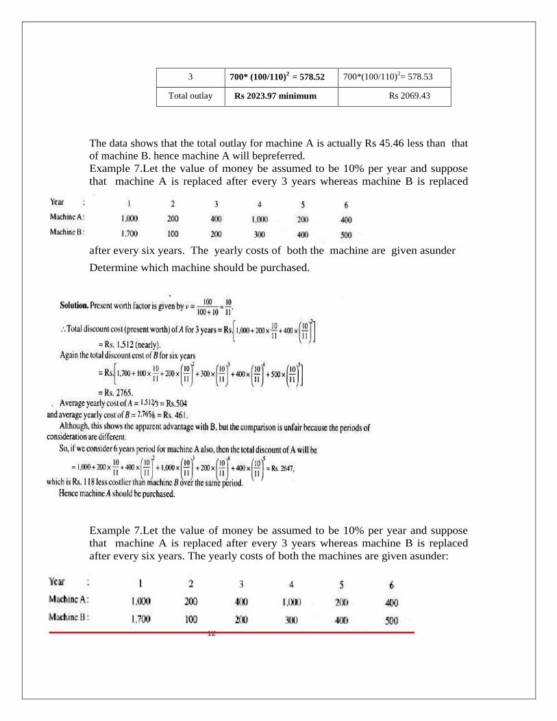
12
3 700* (100/110)2
= 578.52 700*(100/110)2= 578.53
Total outlay Rs 2023.97 minimum Rs 2069.43
The data shows that the total outlay for machine A is actually Rs 45.46 less than that
of machine B. hence machine A will bepreferred.
Example 7.Let the value of money be assumed to be 10% per year and suppose
that machine A is replaced after every 3 years whereas machine B is replaced
after every six years. The yearly costs of both the machine are given asunder
Determine which machine should be purchased.
Example 7.Let the value of money be assumed to be 10% per year and suppose
that machine A is replaced after every 3 years whereas machine B is replaced
after every six years. The yearly costs of both the machines are given asunder:

12
etermine which machine should be purchased.
Example-8: A manual stamper currently valued at Rs 1000 expected to last two years
and Rs 4000 per year to operate. An automatic stamper which can be purchased for
Rs 3000 will last for four years and can be operated at an annual cost of rs 3000. If
money carries the rate of interest10% per annum. Determine which stamper should
bepurchased.
Solution: The present worth factor is given by V = (100)/(100+10)= 0.9091.
The two given stampers have different expected lives, so we shall consider a span of
four years during which we have to purchase either two manual stampers (the second
one being purchased in the third year) or one automaticstamper
YEAR-1 YEAR-2 YEAR-3 YEAR-4
MANUAL STAMPER 1000+4000 + 4000 1000+4000 +4000
Automatic stamper 3000+3000 +3000 +3000 +3000
We now V = 1/(1+r)
The present worth of investments on the two manual stampers used in 4 years =
= 1000+4000 + (4000)/(1+r) + (1000+4000)/(1+r)2 + 4000/(1+r)
3
= 1000 + 1000V2 + 4000 + 4000V + 4000V
2 +4000V
3
= 1000 ( !+V2) + 4000 (1+V+V
2 +V
3)
= 1000(1+0.90912) + 4000 (1+0.9091 + 0.9091
2 + 0.9091
3) = 15773
The present worth of investments on the automatic stamper for the next 4 years =

12
= (3000+3000)+ 3000V + 3000V2+ 3000V
3= 6000+3000(V+v
2+V
3 ) =
3000+10460= 13460
Since the present worth of future costs for the automatic stamper is less than that of
the manual stamper. It will be more profitable to purchase an automatic stamper.
Example-8: A person considering to purchase a machine for his own
factory. Relevant data about alternative machines are as follows:
Machine A Machine B Machine-C
Present investment(rs) 10000 12000 15000
Total annual cost (Rs) 2000 1500 1200
Life (years) 10 10 10
Salvage value 500 1000 1200
As an adviser to buyer, you have been asked to select the best
machine, considering 12% normal rate of return.
You are given that
i. Single payment present worth factor (pwf) @12% for 10 years =0.322
ii. Annual series present worth factor (pwf) @12% for 10 years =5.650
Solution: the present value of total cost of each of the
three m/cs for a period of 10 years is given asbelow:
Machine Present
investment
(Rs)
Present value of
total annual cost
Present value of
salvage value(Rs)
Net cost
(Rs)
(1) (2) (3) (1+2-3)
A 10000 2000*5.65=11300 50080.322=161 21139.00
B 12000 1500*5.65 = 8475 1000*0.322= 322 20153.00 min i
C 15000 1200*5.65= 6780 1200*0.322=
386.40
21393.60
From the above table we conclude that the net cost for m/c-B is the least and
hence the machine B should be purchased.
REPLACEMENT POLICY WHEN THE MAINTENANCE COST
INCREASES WITH TIME AND MONEY VALUE CHANGES WITH
CONSTANT RATE

12
Andsubstitutinginthisformulan=n
How to Select the Best Machine?
In the problem of choosing a best machine (or item), the costs that are constant
over timefor each given machine will still have to be taken into account, although
these costs may differ
foreachmachine
.Onlythosecoststhataresameforthemachinesundercomparisoncanbeexcluded.
Suppose two machines MI and M2 are at our choice. The data required for
determining the best
replacementageofeachtypeofmachineisalsogivenfrompastexperience.Thus,abestsele
ction can be done by adopting the following outlinedprocedure:
Step 1. First find the best replacement age for machine MI and M2both by using
the relationship:
SupposetheoptimumreplacementageformachinesMIandM2comes out be
nl and
n2’respectively.
Step 2. Compute the fixed annual payment (or weighted average cost) for each
machine by using theformula:
1formachineM1andn
=n2 for machine M2. Let it be XI and X2 for machines MI andM2, respectively.
Step 3.
i. If X1<X2’then choose machineMI,
ii. If XI>X2, then choose machineM2.
iii. If XI=X2’then both machines are equally good.
problem-10: a manufacturer is offered two machines a and b. a is priced at rs 5000

12
and running costs are estimated at Rs 800 for each of the first five years, increasing
by Rs200 per year in the sixth and subsequent years. Machine B, which has the same
capacity as A costs s 2500 but will have running costs of Rs 1200 per year for six
years, increasing by Rs 200 per year there after. If money is worth 10% per year,
which machine shold be purchased? (assume that machine will eventually be sold for
scrap at negligibleprice.)
Solution: since the money is worth 10% per year
The discount rate is given by V= 1/(1+r)= 1/(1+0.10) = 0.9091
Therefore , the optimum replacement age ,n, must satisfy the relationship.
For Machine A: for the best replacement age ‘n’, tabulate the required calculations of
Total maintenance cost machine-A in ntable-1
year (n) Running cost
(Rn)
Pwf
(Vn-1
)
(Vn-1
).Rn F(n)=(C-S) +
∑ 𝑅𝑛. 𝑉𝑛 − 1
∑ 𝑉𝑛 − 1 Weighted average
F(n) / ∑ 𝑉𝑛 − 1
1 800 1.000 800 5800 1.0000 5800
2 800 0.9091 737 6537 1.9091 3419
3 800 0.8264 661 7198 2.7355 2628
4 800 0.7513 601 7799 3.4868 2234
5 800 0.6830 546 8345 4.1698 19999
6 1000 0.6209 621 8966 4.7907 1896
7 1200 0.5645 677 9643 5.3552 1799
8 1400 0.5132 718 10361 5.8684 1764
9 1600 0.4665 746 11107 6.3349
10 1800 0.4241 763 11870 6.7590 1755
R10>
F(9)/9
>R9
1800
>
1752
>
1600
It is observed that R10= 1800 becomes greater than the weighted average cost Rs1752
for nine years. Hence. It would be best to replace machine A after nine years; and also
from table1, the equivalent fixed annual payment for machine A is read from last
1752

12
column as x1= weighted average for nine years = Rs1752
Calculations for machine B are shown in table-2
year (n) Running
cost (Rn)
Pwf
(Vn-1
)
(Vn-1
).Rn F(n)=(C-S) +
∑ 𝑅𝑛. 𝑉𝑛 − 1
∑ 𝑉𝑛 − 1 Weighted average
F(n) / ∑ 𝑉𝑛 − 1
1 1200 1.000 1200 3700 1.0000 3700
2 1200 0.9091 1091 4791 1.9091 2510
3 1200 0.8264 991 5782 2.7355 2114
4 1200 0.7513 902 6684 3.4868 1917
5 1200 0.6830 820 7504 4.1698 1800
6 1200 0.6209 745 8249 4.7907 1722
7 1400 0.5645 790 9039 5.3552 1668
8 1600_> 0.5132 821 9860 5.8684 1680
9 1800 0.4665 840 10700 6.3349 1689
Similarily, best replacement age for machine B can be calculated . Since R9>
weighted average for 8 years
1800 > 1680
It would be best to rteplace machine after 8 years.
The equivalent fixed annual payment for machine B is read from table-2 as X2 =
weighted average for 8 years = Rs 1680
Since X1isgraterthanX2, it would be better to purchase machine B instead of machine A
GROUP REPLACEMENT OF ITEMS THAT FAIL COMPLETELY
Group replacement is concerned with those items that either work or fail completely.
It often happens that a system encounters a ;large number of identical low cost items
that are increasingly liable to failure with age. In such cases there is setup cost per
replacement that is independent of the number replaced and it may be advantageous to
replace all items at fixed intervals. Such a policy is called group replacement policy
and is particularly attractive when the value of any individual item is so small that
the cost of keeping records of individual ages
cannotbejustified.Theclassicalexampleofsuchapolicyisusedinreplacinglightbulbs.
Two types of replacement policies are considered
i. Individual replacement: under this policy an item is replaced immediately
after its failure.
ii. Group replacement: under this policy decision is taken as to when all the
items must be replaced, irrespective of the fact that items have failed and
have not failed, with the provision that if any item fails before the optimum
time, it may be replaced individually.
Group Replacement Policy Theorem

12
a. One should group replace at the end of ith
period, if the cost of
individual
replacementsfortheith
periodisgreaterthantheaveragecostperperiodthroug
h the end of ith
period.
b. One should group replace at the end of ith
period , if the cost of
individual replacements at the end of (i-1)th
period is less thanthe
average cost per period through the end of ith
period.
Problem:11 The following failure rates have been observed for a certain type of
light bulbs.
There are 1000 bulbs in use and it costs Rs 10 to replace an individual bulbs
which has burn out. If all the bulbs were replaced simultaneously it would cost
Rs 4 per bulb. It is proposed to replace all bulbs at fixed intervals of time,
whether or not they have burn out, and to continue replacing burnt out bulbs as
and when they fail. At what intervals all the bulbs should be replaced? At what
group replacement price per bulb would on policy of strictly individual
replacement become preferable to the adoptedpolicy.
Solution: Let Pi be the probability that a light bulb, which was new when placed in position for use
fails during the ith
week of its life.
Thus he following frequency distribution is obtained assuming to replace burnt out bulbs as and
when they fail.
P1 = the probability of failure in Ist week = 10/100 = 0.10
P2 = the probability of failure in IInd week = (25-10)/100 = 0.15
P3 = the probability of failure in IIIrd week = (50-25)/100 = 0.25
P4 = the probability of failure in IVth week = (80-50)/100 = 0.30
P5 = the probability of failure in Vth week = (100-80)/100 = 0.20
Total =1.00
Since the sum of all probabilities can never greater than unity, therefore further probabilities P6, P7,
P8 and so on, Thus a bulb that has already lasted four weeks is sure to fail during the fifth week.
Furthermore, assume that
i. Bulbs that fail during a week are replaced just before the end of that week.
ii.The actual percentage of failure during a week for a sub population of bulbs with same age is the
week 1 2 3 4 5
percent failing by
end of the week
10 25 50 80 100

12
same as the expected percentage of failures, during the week for that population.
Let Ni = be the number of replacements made at the end of ith
week, if all 1000 bulbs are new
initially.
Thus N0 = No = 1000
N1 = N0 P1 = 1000 * 0.10 = 100
N2 = N0 P2 + N1 P1 = 1000 * 0.15 + 100 * 0.10 = 160
N3 = N0 P3 + N1 P2 + N0 P2 + N2 P1
= 1000 * 0.25 + 100 * 0.15 + 160 * 0.10 = 281
N4 = N0 P4 + N1 P3 + N2 P2 + N3 P1
= 1000 * 0.30 + 100 * 0.25 + 160 * 0.15 + 281 * 0.10 = 377
N5 = N0 P5 + N1 P4 + N2 P3 + N3 P2 N4 + N4 P1 = 350
N6 = N0 P6+ N1 P5 + N2 P4 + N3 P3 + N4 P2 + N5 P1 = 230
N7 = N0 P7 + N1 P6 + N2 P5 + N3 P25 + N4 P3 + N5 P2 + N6 P1 = 286 and so on
It has been observed that the expected number of bulbs burnt out in a week increases until 4th
week
and then decreases until 6 th week and again starts increasing. Thus the number will continue to
oscillate and ultimately the system settles down to a steady state in which the proportion of bulbs
failing in each week is the reciprocal of their average life.
The mean age of bulbs = 1 * P1 + 2 * P2 + 3 * P3 + 4 * P4 + 5 * P5
= 1* 0.10 + 2 * 0.15 + 3* 0.25 + 4 * 0.30 + 5 * 0.20 = 3.35 weeks
The number of failures in each week in steady state becomes = 1000/3.35 = 299
The cost of replacing bulbs individually only on failure = 10* 299 = 2990 @ 10 per bulb
Since the replacement of all 1000 bulbs simultaneously costs Rs 4 per bulb and replacement of an
individual bulb on failure costs Rs10
Therefore the cost of replacement of all bulbs simultaneously is as given in following table:
End of
week
Cost of individual
replacement)
Total cost of group
replacement
Average cost per week

12
1 100 nos * 10 = 1000 1.000 * 4 + 100*10 = 5000 5000/1 = 5000
2 160 nos* 10 = 1600 5000 + 160 *10 = 6600 6600/2 = 33000
3 281 *10 = 2810 6600 + 281 * 10 = 9410 9410/3 = 3136.6
4 377 * 10 = 3770 9410 + 377 *10 = 13180 13180/4= 3294.80
The cost of individual replacement in the 4th
week exceeds the average cost for 3 weeks.
Thus it would be optimal to replace all the bulbs after every 3 weeks other wise average cost will
start increasing. Further , since the group replacement at the end of one week costs Rs5000, and
the individual replacement after one week cost Rs 2990, the individual replacement is preferred.
Problem-13: A computer contains 10000 resisters. When any one of the resistor fails, it is
replaced. The cost of replacing a single resistor is Rs 10 only. If all the rsistors are replaced at the
same time, the cost per resistor would be reduced to Rs 3.50. the percent surviving by the end of
moth is as follows:
Problem-13: A computer contains 10000 resisters. When any one of the resistor fails,
it is replaced. The cost of replacing a single resistor is Rs 10 only. If all the rsistors
are replaced at the same time, the cost per resistor would be reduced to Rs 3.50. the
percent surviving by the end of moth is as follows:
What is the optimum plan?
Solution: the probabilities Pt of failure during the month t are
P1= the prob of falure in Ist month = (100-97) /100 = 0.03
P2= the prob of falure in 2nd
month = (97-90) / 100 = 0.07
P3 = the prob of falure in 3rd month = (90-70) /100 = 0.20
P4 = the prob of falure in 4th
month = (70-30) /100 = 0.40
Month 0 1 2 3 4 5 6
% surviving by the
end of the m end of month
100 97 90 70 30 15 0
Month 0 1 2 3 4 5 6
% surviving by the
end of the m end of month
100 97 90 70 30 15 0

12
P5 = the prob of falure in 5th
month = (30-15 ) / 100 = 0.15
P6= the prob of falure in 6th
month = (15-0 0 /100 = 0.15
1∑ 𝑷𝒕𝟔𝒕=𝟏 = 1.0
Let Nt = be the number of replacements made at the end of tth
monthif all 10000 resistors are new
initially. .
thus N0 = No = 10000
N1 = N0 P1 = 10000 * 0.03 = 300
N2 = N0 P2 + N1 P1 = 10000 * 0.07 + 300 * 0.03 = 709
N3 = N0 P3 + N1 P2 + N0 P2 + N2 P1
= 10000 * 0.20 + 300 * 0.07 + 709 * 0.03 = 2042
N4 = N0 P4 + N1 P3 + N2 P2 + N3 P1 = 4171
N5 = N0 P5 + N1 P4 + N2 P3 + N3 P2 N4 + N4 P1 = 2030
N6 = N0 P6+ N1 P5 + N2 P4 + N3 P3 + N4 P2 + N5 P1 = 2590 and so on
Average life of each resistor = 𝑖 = 6 ∑ 𝑖 𝑃𝑖𝑖=1 =
It has been observed that the expected number of bulbs burnt out in a week increases until
4th
week and then decreases until 6 th week and again starts increasing. Thus the number
will continue to oscillate and ultimately the system settles down to a steady state in which
the proportion of bulbs failing in each week is the reciprocal of their average life.
= 1 * P1 + 2 * P2 + 3 * P3 + 4 * P4 + 5 * P5 + 6 * P6
= 1 * 0.03 + 2 * 0.07 + 3 * 0.20 + 4 * 0.40 + 5 * 0.15 + 6 * 0.15
= 0.03 + 0.14 + 0.60 + 1. + 0.75 + 0.90 = 4.02 months
Average life of each resistor = 4.02 months
Average no. of replacements every month = 10000/4.02 = 2488
Average cost of monthly individual replacements = 2488 * 10 = 24880
Under group replacement we find
End of
month
Cost of individual
replacement
Total cost of group replacement
Average cost per month
1 300 nos * 10 = 3000 10000 * 3.5 + 300*10 = 38000 38000/1 = 38000
2 709 nos* 10 = 7090 38000 + 709 * 10 = 45090 45090 /2 = 22545
3 2042 *10 = 20420 45090 + 2042 * 10 = 65510 65510 /3 = 21836.66
4 4171 * 10 = 41710 65510 + 4171 * 10 = 107220 107220/ 4 = 26805.00

12
The cost of individual replacement in the fourth month exceeds the average cost for 3 months.
hence it would be optimal to replace all the resistors after every 3 months, otherwise the average
cost will start increasing. *** **
*****
UNIT-IV
THEORY OF GAMES AND INVENTORY
Game Theory covers the following concepts
Game TheoryIntroduction
Minimax criterion ofoptimality
Games without saddlepoint
Introduction
Life is full of struggle and competitions. A great variety of competitive situations
is commonly seen in everyday life. For example, candidates fighting an election
have their conflicting interests, because each candidate is interested to secure
more votes than those secured by all others. Besides such pleasurable activities in
competitive situations, we come across much more earnest competitive
situations, of military battles, advertising and marketing campaigns by competing
business firms,etc.
What should be the bid to win a big Government contract in the pace of
competition from several contractors? Game must be thought of, in a broad sense,
not as a kind of sport but as competitive situation, a kind of conflict in which
somebody must win and somebodymustlose.
Game theory is a type of decision theory in which one’s choice of action is

12
determined after taking into account all possible alternatives available to an
opponent playing the same game, rather than just by the possibilities of several
outcomes. The game theory has only been capable of analysing very simple
competitive situations. Thus, there has been a great gap between what the theory
can handle and most actual competitive situations in industry and elsewhere. So
the primary contribution of game theory has been its concepts rather than its
formal application to solving realproblems.
Game is defined as an activity between two or more persons involving activities
by each person according to a set of rules at the end of which each person receives
some benefit or satisfaction or suffers loss (negative benefit). The set of rules , at
the end of which each person receives some benefit or satisfaction or suffers loss (
negative benefit).
Characteristicsof Game Theory
There can be various types of games. They can be classified on the basis of the
following characteristics.
i. Chance of strategy: If in a game, activities are determined by skill, it is said to
be a game of strategy; if they are determined by chance, it is a game of chance.
In general, a game may involve game of strategy as well as a game of chance. In
this chapter, simplest models of games of strategy will beconsidered.
ii. Number of persons: A game is called an n-person game if the number of persons
playing is 11.The person means an individual or a group aiming at a particular
objective.
iii. Number of activities: These may be finite or infinite.
iv. Number of alternatives (choices) available to each personin a particular
activity may also be finite or infinite .A finite game has a finite number of
activities, each involving a finite number of alternatives, otherwise the game is
said to beinfinite..
v. Information to the players about the past activities ofother players is
completely available, partly available, or not available atall.
vi. Payoff: A quantitative measure of satisfaction a person gets at the end of each
play iscalled a payoff. It is a real-valued function of variables in thegame.
Let vi be the payoff to the player Pi,
1<i <n, in an n person game. If , then the game is said to be a zero-sum
In this lesson, we shall discuss rectangular games (also called two- person zero-
sum).
BasicDefinitions
game.

12
at each pla
1. Competitive Game. A competitive situation is called a competitive game if it has the following fourproperties:
i. There are finite number (n) of competitors (called players) such that n~2. In case
n=2, it is called a two- person game and in case n>2, it is referred to as an n-
persongame.
ii. Each player has a list of finite number of possible activities (the list may not be
same for eachplayer).
iii. A play is said to occur when each player chooses one of his activities. The
choices are assumed to be made simultaneously, i.e. no player knows the choice
of the other until hehas decided on hisown.
iv. Every combination of activities determines an outcome (which may be points,
money or anything else whatsoever) which results in again of payments(+ ve, - ve
or zero) to each player, provided each player is playing uncompromisingly to get
as much as possible. Negative gain implies the loss of sameamount.
v. Value of game: it is the expected gain of player A , if bothplayers use their best
strategies.
We define best strategy on the basis of the minimax criterion of optimality.
Saddle Point: a saddle point is an element of the matrix which is both the
smallest element in its row and thelargest element in its column,
2. Zero-sum and Nonzero-sumGames:
.Competitive games are classified according to the number of players in volved,
i.e. as a two person game.. three person game, etc. Another important distinction
isbetween zero-sum games and nonzero-sum games. If the players make payments
only to each other, i.e. the loss of one is the gain of others, and nothing comes
from outside, the competitive game is said to bezero-sum.
Mathematically, suppose an n-person game is played by n players P1, P2 ‘..., P”
whose respective pay-offs at the end of a play of the game are VI ,V2, ... V”then,
the game will be called zero- sum
y of the game. A game which is not
zero-sum is called a nonzero-sum game. Most of the competitive games are zero-
sum games. An example of a nonzero-sum game is the ‘poker’ game in which a
certain part of the pot is removed from the ‘house’ before the finalpayoff.
3. Strategy: A strategy of a player has been loosely defined as a rule for decision-
makingin advance of all the plays by which he decides the activities he should
adopt. In other words, a strategy for a given player is a set of rules (programmes)
that specifies which of the available course of action he should make at eachplay.

12
This strategy may be of two kinds:
i. Pure Strategy.: If a player knows exactly what the other player is going to do, a
deterministic situation is obtained and objective function is to maximize thegain.
Therefore, the pure strategy is a decision rule always to select a particular
course of action. A pure strategy is usually represented by a number with which
the course of actionis associated.
ii. Mixed Strategy.[Agra92; Kerala (Stat.) 83]: If a player is guessing as to which
activity is to be selected by the other on any particular occasion, a probabilistic
situation is obtained and objective function is to maximize the expectedgain.
Thus, the mixed strategy is a selection among pure strategies with fixed
probabilities.
Mathematically, a mixed strategy for a player with m (:2:2) possible courses of
action, is denoted by the set S of m non-negative real numbers whose sum is
unity, representing probabilities with which each course of action is chosen. If
Xi(i =I, 2, 3, ..., m) is the probability of choosing the course i, then
4. Two-Person, Zero-Sum (Rectangular) Games. A game with only two players
(say, Player and Player B) is called a ‘two- person, zero-sum game’ if the losses
of one player
areequivalenttothegainsoftheother,sothatthesumoftheirnetgainsiszero.
Two-person, zero-sum games are also called rectangular games as these are
usually represented by a payoff matrix in rectangular form.
5. Payoff Matrix. Suppose the player A has m activities and the player B has n
activities. Then a payoff matrix can be formed by adopting the followingrules:
i. Row designations for each matrix are activities available to playerA.
ii. Column designations for each matrix are activities available to playerB.
iii. Cell entry ‘vij, is the payment to player A in A’spayoff matrix when A chooses the
activity
i and B chooses the activity j.
iv. With a ‘zero-sum, two person game’, the cell entry in the player B’ s payoff
matrix will be negative of the corresponding cell entry ‘Vi}, in the player A’s
payoff matrix so that sumof payoff matrices for player A and player B is
ultimatelyzero.

12
In order to make the above concepts a clear, consider the coin matching game
involving two players only. Each player selects either a head H or a tail T. If the
outcomes match (H, H or T, T), A wins Re 1from B , otherwise B wins Re 1from
A . This game is a two-person zero-sum game. since the winning of one player is
taken as losses for the other. Each has his choices between two pure strategies (H
or T). This yields the following (2 x 2) payoff matrix to player A.
It will be shown later that the optimal solution to such games requires each player
to play one pure strategy or a mixture of purestrategies.
Assumptions of the Game:
each player has available to him a finite number of possible strategies (course of
action). The list may not be the same for each player.
Player act rationally andintelligently.
List strategist of each player and the amount of gain or loss on individual’s choice
of strategy is known to each player inadvance.
One player attempts to maximize gains and the other attempts to minimizelosses.
Both players make their decisions individually, prior to the play, without direct
communication betweenthem.
Both players select and announce their strategies simultaneously so that neither
player has an advantage resulting from the direct knowledge of the other
player’sdecision.
The payoff is fixed and determined inadvance.
Minimax (Maximin) Criterion And Optimal Strategy The ‘minimax criterion
of optimality’ states that if a player lists the worst possible outcomes of all his

12
potential strategies, he will choose that strategy to be most suitable for him
which corresponds to the best of these worst outcomes. Such a strategy is called
an optimalstrategy.
Problem-1:Consider (two-person, zero-sum) game matrix, which represents
payoff to the player A. Find, the optimal strategy, if any.(See Table)
PLAYER - B
PLAY
ER
-A
I II III
I -3 2 6
II 2 0 2
III 5 -2 -4
Solution; the player A wishes to obtain the larsest possible ‘Vij’ by choosing one of his
activities (I, II,III),
while the player B is determined to make A’s gain the minimum possible by choice of
activities from his list (I, II, III). Then the player A is called the maximizing player abd
B the minimizing player.
PLAYER - B
PLA
YE
R -A
I II III Row
minimu
m
I -3 2 6 -3 maximin=
max(-3,0,-
)=0
II 2 0 2 0
III 5 -2 -4 -4
Colu
mn
maxi
mum
5 0 6
Minimax value = mini (5,0,6) =0
If the Player A chooses the Ist activity , then it would happen that the player B
also chooses his Ist activity. In this case the player B can guarantee a gain of least -3 ie
mini( -3, -2, 6) =-3
Similarly, for other choices of player A, ie, II and III activities , B can force the
player A to get only o and -4 respectively, by his proper choices from (I, II, III)ieMini
(2.0,2) = 0
Mini (5, -2, -4)=-4

12
-4
The minimum value in each row guaranteed by the player A
is indicated by ‘row minimum’ as shown in thetable.
ThebestchoicefortheplayerAistotomaximizehisleastgains-3,0,-4 = 0 and opt II
strategy which assures at most the gain ‘0’ie’
Max (Row minimum of the strategy I, II, III of B) = Max ( min (-3,-2, 6), min(2,0,2),
min ( 5, - 2, -4))= max( -3, 0, -4)=0
Mini( column Maximum of the strategy I, II,III of A)= mini( max( -3,2,5), max( -2, 0, -
2), max( - 6, 2, -4)= mini( 5,0,2)=0
MaxminiVij= Mini max Vij=0 i j jI Saddle point is ‘o”
Soluion is:
Player A uses his course of action II throughout Player B uses his course of action II
throughout The value of game for player A =0
The value vof game for player B =-0 This game is fair to ,player A and B The solution
to this game is unique. Rules for determining a saddlePoint:
Step-1: select the minimum element of each row of the payoff matrix and mark them by
Spep-2: Select the greatest element of each column of the payoff matrix and mark them
by
Step-3: if there appears an element in the payoff matrixmarkedby and both, the
position of that element is a saddle point of the payoffmatrix.
Example-2: Consider the following game
PLAYER - B
PLAYER
-A
I II III
I 3 -4 8
II -8 5 -6
III 6 -7 6
PLAYER - B
PLAYER
-A
I I I II
I
Row
minim
um
I 3 - 4 8 -4 Maximin=

12
II -
8 5 -6 -8 Maxi(-4,-
8,- 7)= -4
III 6 -7 6 -7
M
a
Colum
n
maxim
u
6 5 8
x m minimax = mini(6,5,8)=5
in=-4, minimax=5 Maxmin#minimax
There is no saddle point for thisgame.
Problem-3. The pay-off matrix for a two person zero-sum game is
given below. Find the best strategy for each player and the value of
thegame.
PLAYE
R - B
PLAYE
R - A
I II III I
V
V
I -2 0 0 5 3
II 3 2 1 2 2
III -4 -3 0 -2 6
IV -4 -3 0 -2 6
V 5 3 -4 -2 -6
Solution:
PLAYE
R - B
PLAYER -
A
I II III IV V row
mini
I -2 0 0 5 3 0
II 3 2 1 2 2 1
II I -4 -3 0 -2 6 -4

12
I V -4 -3 0 -2 6 -4
V 5 3 -4 -2 -
6 -6
Col
max
5 3 1 5 6
maxmin= max( 0,1,-4,-6) = 1
Minimax =
mni
(5,3,1,5,6) =
1 Maxmin=
minimax = 1
The
saddle
point
is 1
Soluti
on is:
Player A uses his course of action II throughout Player B uses his course of action III
throughout The value of game for player A =1
The value vof game for player B =-1 This game is fair to ,player A
The solution to this game is unique.
Problem-4: determine the solution of the following game.
PLAYER - B
PLAYE
R -A
I II III
I -2 15 -2
II -5 -6 -4
III -5 20 -8
PLAYER - B

12
PLAYER -A
I II III Ro
w
mini
mum
I -2 15 -2 -2 Maximin=
Maxi(-2,-6,-
8)= -2
II -5 -6 -4 -6
III -5 20 -
8
-8
col
max
-2 20 -2
minimax = mini(-2,20,-2)=
-2
The Row minima, corresponding to player A’s course of
action I,II and III are -2, -6 and -8 respectively
The column maxima, corresponding to B,s course of action are -2, 20, -2.
The largesr of row minimua and the smallest of the column maxima are both equal to -2.
Here the saddle point is -2. However , there are two elements
whose value is -2 and hence the game has two saddle points.
maxmin= max( -2, -6, -8) = -2
Minimax = mni (-
20, 20, -2) = -2
Maxmin= minimax
= -2
The saddle point is -2
Soluion to such a game is not unique.
Player A uses his course of action I throughout
Player B may uses either of his courses of action I or III throughout, or a mixed
strategy which uses any combination of these courses ofaction.
The value of game for player A = -2 The value of game for player B = +2 This game

12
is fair to ,player B
The solution to this game is not unique.
MIXED STRATEGIS: GAME WITHOUT SADDLE POINT:
In certain cases, there is no pure strategy solution for the game, ie. No saddle point
exists. In such cases, to spolve games both players must determine an optimal
mixture of strategies to find a saddle (Equilibrium) point.
The optimal strategy mixture for each player may be determined by assignibg to
each strategy its probability of being choosen, the strategies , so determined, are
called mixed strategies. This is because they are probabilistic combination of the
available choices ofstrategy.
A mixed strategy game can be solved by following methods.
i. Algebricmethod
ii. Arithmaticmethod
iii. Matrixmethod
iv. Graphicalmethod
v. Linear programmingmethod`
THE RULES (PRINCIPLES) OF DOMINANCE
The rules dominance are used to reduce the size of the payoff matrix. These rules can
help in deleting certain rows and / or columns of the payoff matrix that are inferior (
less attractive) to at least one of the remaining rows and /or columns ( strategies), in
terms of payoff matrix to both the players. Rows and/or columns once deleted can
never be used for determining the optimum strategy for both theplayers.
For p;layer A, who is assumed to be gainer. If ach element in a row, say Rr, is less
than or equal to the corresponding element in another row, say Rs, in the payoff
matrix, then the row Rr is said to be ( inferior) dominated by row Rs, and therefore,
rowRrcan be deleted from the payoff matrix. In other words , player A will never use

12
the strategy corresponding to row Rr, , because he will gain less by choosing such
astrategy.
For p;layer B, who is assumed to be loser, If ach element in a column, say Cr, is
greater than or equal to the corresponding element in another column, Cs, in the payoff
matrix, then the column Cr is said to be ( inferior) dominated by column Cs, and
therefore, column Cr can be deleted from the payoff matrix. In other words , player B
will never use the strategy corresponding to column Cr, , because he will loose more
by choosing suchstrategy.
A strategy say , k can also be dominated if it is inferior ( less attractive) to an average
of two or more other pure strategies. In this case, if the domination is strict, then
strategy k can be deleted
Problem-4: In a game of matchng coins with two players , suppose one player wins Rs
2 when there are two heads and wins nothing when there are two tails; and losses Rs 1
when there are one head and one tail. Determine the payoff matrix , the best strategies
for each player and the value of thegame.
Solution: The pay of matrix for player a is as follows:
PLAYER-B
H T Row
min PLA H 2 -
1 -1 Maximin=
YE prob x Maxi(-2,-6,-8)= -
-
1
R - T
1-
0 -1
2
A x
Column max 2
0
Minimax(2,0) =0
Here Minimax # maximin, so there is no saddle point. We need
to find mixed strategies for each of the player.

12
Let the player A plays H with probability x
ad T with probability 1-x So that sum = 1,
x+ (1-x)=1
Then if the player B plays H all the time,
A’s expected gain will be E(A, H) = 2.x
+ (-1)(1-x)=3x-1 ------------------- eqn-1
Similarly , if the player B plays T all the
time, A’s expectd gain will be E( A, T) = x (-
1) + (1-x). 0 = -x ---------- eqn-2
It can be shown mathematically
that E(A, H) = E
(A, T) 3x -1 = -x
4x =1, x= ¼, 1-x = ¾
Therefore , best strategy for player A is to play H and T with
probability ¼ and ¾ respectively. Since it is a mixed strategy,
the strategy o player A = [ ¼, ¾]
The expected gain for player A = E(A) = (1/4)*2 + (3/4)*(-1) = -1/4
Let the player B plays H with probability y
ad T with probability 1-y Then if the player
B plays H all the time, B’s expected gain
will be E(B, H) = E(B,T)= E(B)SAY
2.y + (-1)(1-y) = 3y -1 ---------- eqn-1
Similarly , if the player A plays T all the
time, B’s expectd gain will be E( B, T) = y (-
1) + (1-y). 0 = -y ---------- eqn-2
It can be shown mathematically
that E(A, H) = E
(A, T) 3y -1 = -y
4y =1, y= ¼, 1-y = ¾
Therefore , best strategy for player B is to play H and T with
probability ¼ and ¾ respectively. Since it is a mixed strategy,
the strategy o player B = [ ¼, ¾]
The expected gain for player B = E(A) = (1/4)*2 + (3/4)*(-1) = -1/4

12
The complete solution of the game is;
The player A should play H and T with
probabilities 1/4, and ¾ respectively. Thus A’s
optimal strategy is ( ¼,¾)
The player B should play H and T with
probabilities ¼ and ¾ respectively Player B’s
optimal strategy is (1/4, ¾)
The expected value of the game for player A = -
1/4
Problem-5:determine the solution of the
following game
PLAYER
- B
PLAYE
R - A
I II III
I 0 -2 7
II 2 5 6
III 3 -3 8
Solution:
PLAYER - B
PLAY
ER
-A
I II III Row
minim
um
I 0 -2 7 -2 Maximin=
Maxi(-2,2,-
3)= -3
II 2 5 6 2
III 3 -3 8 -3
col
maximum
3 5 8
minimax = mini(3,5,8)=
3
Here Minimax # maximin, so there no saddle point
Applying principle of dominance reduce the payoff matrix to 2*2 form
PLAYER
- B
I II II

12
PLAYE
R -A
I
I 0 -2 7
II 2 5 6
III 3 -3 8
On observing Columns Col-III >= Col-I, col-III is inferior or dominated column. So detete col-III
PLAYER - B
PLAYE
R -A
I II
I 0 -2
II 2 5
II
I
3 -3
PLAYE
R - B

12
Observing rows Row-1 is <= Row-II ie Row-1 is inferior to
Row-II , Delete Row-1
Here Minimax # maximin, so there is no saddle point. We need to find mixed
strategies for each of the player.
Let the player A plays strategy II with probability x and Strategy III with probability
1-x So that sum = 1, x+ (1-x)=1
TheniftheplayerBplaysStrategyIallthetime,A’sexpectedgainwillbe E(A, II) = 2.x +
3(1-x)=3-x -------------------- eqn-1
Similarly , if the player B plays Strategy II all the time, A’s expectd gain will be E( A,
III ) = 5 x + (1-x). (-3) = 8x-3----------eqn-2 B’s Istrategy
It can be shown mathematically that E(A, I) = E(A,II) B’s II strategy 3-x =8x-3,
x =6/9
Therefore , best strategy for player A is to play Strategy II and strategy III with probability 2/3 and 1/3 respectively. Since it is a mixed strategy, the strategy of player
A = [0, 6/9, 3/9]
The expected gain for player A = E(A) = (6/9)2 + (3/9)3 = 4/3 +1= 7/3
Let the player B plays Strategy I with probability y and strategy II with probability 1-
y Then if the player B plays Strategy I all the time, B’s expected gain will be
2.y + 5(1-y) = 5- 3y ---------- eqn-1
Similarly , if the player B plays strategyT all the time, B’s expectd gain will be E( B,
II) = 3 y -3 (1-y) = 6y-3---------- eqn-2
It can be shown mathematically that E(A, I) = E (A, II) 5-3y = 6y-3
9y =8, y= 8/9, 1-y = 1/9
The expected gain for player B = E(A) = 2* 8/9 + 5 * 1/9 = 21/9 The complete
solution of the game is;
A’s optimal strategy is [ 0, 8/9, 1/0]
Player B’s optimal strategy is [ 8/9, 1/9, 0 ]
The expected value of the game for player A = 19/9
PLAYER -
A
I II
II 2 5
III 3 -3

12
Problem-5:determine the solution of the following game
PLAYER
- B
PLAYE
R -A
I II III
I 6 1 3
II 0 9 7
III 2
4
PLAYER
- B
PLAYE
R -A
I II III Row
min
im
um
I 6 1 3
1 Maximin
=
Maxi(1,
0,2)= 2
II 0 9 7 0
III 2 3 4 2
colmn max 6 9 7
minimax = mini(6,9,7)=
6
Max Min # minimax, so there is no saddle point.
PLAYER - B
PLAYER -A
I II III
I 6 1 3
II 0 9 7
III 2 3 4
This has no saddle point.
Further none of the pure strategies of A is inferior to any of his other pure strategies.
However average of A’s first & second pure strategies gives us

12
Row-III <= ( average of row –I and row-II) (0 , 9, 7) <= [ ( 6+0)/2, (1+9)/2, (3+7)/2]
[ 0, 9, 7 ] <= [ 3, 5, 5 ]. , row-III is inferior to other rows, deleteRow-III
PLAYER - B
PLAYER -A
I II III
I 6 1 3
II 0 9 7
III 2 3 4
Problem :6 Solve the following game and find the value of game:
Row-1 <= Row-III
( 3, 2, 4, 0 ) <= ( 4, 2, 4, 0 ) delete Row-1
PLAYER - B
PLAYER -A
I II III IV
II 3 4 2 4
III 4 2 4 0
IV 0 4 0 8
Col –I >= col-III, detete col-I
col-I
col-III
3 2
PLAYE
R - B
PLAYE
R -A
I II III IV
II 3 4 2 4
III 4 2 4 0
IV 0 4 0 8

12
4 =
4
Column II >= Avg of Col III % col IV
II
>
=
Avg col
III &IV
PLA
YER
-A
II 4 (2+4)/2=3
III 2 (4+0)/2=
2
IV 4 (0+8)/2=4
Delete col-II
PLA
YER
-A
III IV
II 2 4
III 4 0
IV 0 8
Row-II <= Avg of Row III & row IV
[ 2, 4 ] <= [ ( 4+0)/2, (0+8)/2]
[ 2, 4 ] <= [ 2, 4] delete row-II
PLA
YER
-A
III y=2/3 IV
1-y=1/3
III x=2/3 4 0
IV
1-x=1/3
0 8
4x + 0* (1-x) = 0*x + 8 (1-x), 4x+8 x =8, 12x =8 , x= 2/3
4y + 0*(1-y) = 0.y + 8 * (1-y)
4y+ 8y = 8, y = 8/12 = 2/3
Strategy of player A = ( 0, 0, 2/3, 1/3)
Strategy of player B = ( 0, 0, 2/3, 1/3)
Value of game for player A = 2/3*4 = 8/3
GRAPHICAL METHODS FOR (2*n and m*2 ) GAMES

12
Problem-7: Solve the following (2 X 3) game graphically
PLAYER - B
PLAYER -A
y1
I
y2
II
y3
III
I x1 1 3 11
II 1-x1 8 5 2
Solution: Max( Row min ) = Max ( 1, 2) =1
Mini (col max) = mini ( 8, 5, 11 ) =8
Maxmin # minmax
This game does not have a saddle point.
Thu the player A’s expected pay-off corresponding to the player B’s pure strategies are given in
following table-1
Three expected payoff lines are :
B’s Pure
strategies
A’s Expected payoff E(x1)
I E(x1) = 1x1 + 8(1-x1) = -7x1 + 8
II E(x1) = 3.x1 + 5(1-x1) = -2x1 + 5
III E(x1) = 11x1 + 2(1-x1) = 9x1 + 2
E(x1) = -7x1 + 8
E(x1) = -2x1 + 5
E(x1) = 9x1 + 2 and can be plotted on a graph as follows
First draw two parallel lines one unit apart and mark a scale on each. These two lines will
represent two strategies available to the player A. then draw lines to represent each of
player B’s strategies.
For example, to represent the player B’s Ist strategy, join mark 1 on scale Iand mark 8 on
scale II.
To represent the player B’s second strategy, join mark 3 on scale I & mark 5 on scale II
and so on.
Since the expected pay-off E(x1) is a function of x1 alone, these three expected pay-off
lines can be drawn by taking x1 as x-axis and E(x1) as y-axis

12
Points A, P,B,C on the lowest boundary represent the lowest possible expected gain to the
player A for any value of x1 between 0 and 1. According to the maximum criterion, the player A
chooses the best of these worst outcomes.
Clearly, the highest point P on the lowest boundary will give the largest expected gain PN to A. so
the best strategies for the player B are those which pass through the point P. thus the game is
reduced to 2 x 2 as shown in table-2.
PLAYER - B
PLAYER -
A
y2
II
y3
III
I x1 3 11
II 1-x1 5 2

12
Considering player-A 3x1 + 5(1-x1) = 11x1 + 2(1-x1) ,
3x1+5 - 5x1 = 11x1 + 2- 2x1
3x1-5x1 -11x1 +2 x1 = 2-5
- 11x1 = -3 x1 = 3/11
Considering player-B
- 3y2 + 11(1-y2) = 5y2 + (1-y2) 2
3y2 +11-11y2 = 5y2 +2 -2y2
3y2 -11y2 -5y2 +2y2 = 2 -11 -11y2 = -9
Y2 = 9/11
Y3 = (1-y2) = 2/11
The solution of the game is obtained as follows:
The player A choose optimal mixed strategy ( x1, x2 )= (3/11, 9/11)
The player B choose optimal mixed strategy ( y1, y2 , y3)= ( 0, 2/11, 9/11)
The value of game to the player A is V = 49/11
V(A) = 3*3/11 + 5*8/11 = 49/11
Problem-8: solve the game graphically whose payoff matrix for player A is given as follows:
PLAYER - B
PLAYER -A
y1
I
y2
II
I x1 2 4
II 1-x1 2 3
III 3 2
IV -2 6
Solution:
Max( min rows) = max( 2,2,2,-2) =2
Min(max colums) = Min( 3, 6) = 3
Maxmin # mimax , hence there is no saddle point
The game does not have a saddle point,
Let y1 and y2 (= 1-y1) be mixed strategies of the player B
Thu the player B’s expected pay-off corresponding to the player A’s pure strategies are given in following table-1
Four expected payoff lines are :

12
A’s Pure strategies B’s Expected payoff E(x1)
I E(y1) = 2y1 + 4(1-y1) = -2y1 + 4
II E(y1) = 2.y1 + 3(1-y1) = -y1 + 3
III E(y1) = 3y1 + 2(1-y1) = y1 + 2
IV E(y1) = -2y1 + 6(1-y1) = -8y1 + 6
E(y1) = -2y1 + 4
E(y1) = -y1 + 3
E(y1) = y1 + 2
E(y1) = -8y1 + 6 and can be plotted on a graph as follows
First draw two parallel lines one unit apart and mark a scale on each. These two lines will
represent two strategies available to the player B. then draw lines to represent each of player A’s
strategies.
For example, to represent the player A’s Ist strategy, join mark 2 on scale Iand mark 4 on scale II.
To represent the player A’s second strategy, join mark 2 on scale I & mark 3 on scale II and so
on.
Since the expected pay-off E(y1) is a function of y1 alone, these four expected pay-off lines can
be drawn by taking y1 as x-axis and E(y1) as y-axis
In this case, the minima point is determined as the lowest point PointP on the

12
uppermost boundary. Lines intersecting at the minimax point P correspond to the
player A’s pure strategies I and III. This indicates x2 = 0, x4 =0. Thus the reduced
game is given in table-2.
Clearly, the lowest point P on the highest boundary will give the lowest expected
gain PN to B. so the best strategies for the player A are those which pass through
the point P. thus the game is reduced to 2 x 2 as shown in table-2.
PLAYER - B
PLAYER -A
y1
I
y2
II
I x1 2 4
III 1-x1 3 2
Considering player-A 2x1 + 3(1-x1) = 4x1 + 2(1-x1) ,
2x1+3 - 3x1 = 4x1 + 2- 2x1
2x1-3x1 -4x1 +2 x1 = 2-3
- 3x1 = -1 x1 =1/3 , 1-x1 = 2/3
- Considering player-B 2y1 + 4(1-y1) = 3y1 + (1-y1) 2
2y1 + 4 - 4y1 = 3y1 +2 -2y1
2y1-4y1 -3y1 +2y1 = 2 -4 -3y1 = -2
Y1 = 2/3
Y2 = (1-y1) = 1/3
Value of game for player A = 2*1/3 + 3 *2/3 = 8/3
The solution of the game is obtained as follows:
The player A choose optimal mixed strategy ( x1, x2, x3, x4 )= (1/3, 0, 2/3, 0)
The player B choose optimal mixed strategy ( y1, y2 )= ( 2/3, 1/3 )
The value of game to the player A is V = 8/3
V(A) = 2*1/3 + 3*2/3 = 8/3
------ ** -----

12
INVENTORY
This chapter will focuses on following concepts.
InventoryIntroduction
InventoryModel
Introduction
Definition:
The function of directing the movement of goods through the entire
manufacturing cycle from the requisitioning of raw materials to the inventory of
finishes goods orderly mannered to meet the objectives of maximum customer-
service with minimum investment and efficient (low-cost) plantoperation.
What Is Inventory?
In broad sense, inventory may be defined as the stock of goods, commodities or
other economic resources that are stored or reserved in order to ensure smooth and
efficient running of businessaffairs.
The inventory or stock of goods may be kept in any of the following forms:
i. Raw material inventory, i.e. raw materials which are kept in stock forusing in the
productionof\goods.
ii. Work-in-process inventory, i.e. semi finished goods or goods in process, which
are storedduring the productionprocess.
iii. Finished goods inventory, i.e. finished goods awaiting shipment from the factory.
iv. Inventory also includes furniture, machinery, fixtures, etc. The term inventory
may be classified in two main categories. Reasons for carrying Inventory:
i. To improve customerservice
ii. To reduce operatingcosts
iii. Maintenance of operationalcapability
iv. To manage irregular supply anddemand.
v. To avail quantitydiscounts.
vi. Avoidingstockouts(shortages) 1- DirectInventories
The items which playa direct role in the manufacture and become an integral part
of finished goods are included in the category of direct inventories. These may be
further classified into four main groups:
a. Raw material inventories are provided:

12
i. for economical bulk purchasing,
ii. to enable production rate changes
iii. to provide production buffer against delays in transportation,
iv. for seasonal fluctuations.
b. Work-in-process inventories are provided:
i. to enable economical lot production,
ii. to cater to the variety of products
iii. for replacement of wastages,
iv. to maintain uniform production even if amount of sales may vary.
c. Finished-goods inventories are provided:
i. for maintaining off-self delivery,
ii. to allow stabilization of the production level
iii. for sales promotion.
d. Spare parts. IndirectInventories
Indirect inventories include those items, which are necessarily required for
manufacturingbut do not become the component of finished production, like: oil,
grease, lubricants, petrol, and office-material maintenance material,etc.
Types of Inventory Models
Basically, there are five types of inventory models:
i. Fluctuation Inventories: These have to be carried because sales and production
times cannot be predicted accurately. In real-life problems, there are fluctuations
in the demand and lead- times that affect the production of items. Such types of
reserve stocks or safety stocks are called fluctuation inventories.
ii. Anticipation Inventories : .These are built up in advance for the season of large
sales, a promotion programe or a plant shutdown period. In fact, anticipation
inventories store them en and machine hours for futurerequirements.
iii. Cycle (lot-size) inventories. In practical situations, it seldom happens that the rate
of consumption is the same as the rate of production or purchasing .So the
items are procured inlargerquantitiesthantheyarerequired.Thisresultsincycle(orlot-
size)inventories.
iv. Transportation Inventories : .Such inventories exist because thematerials are
required to move from one place to another. When the transportation time is long,
the items under transport cannot be served to customers. These inventories exist
solely because of transportationtime.
v. Decoupling Inventories: Such inventories are needed for meeting out the demands
during the decoupling period of manufacturing or purchasing.
Inventory Decisions

12
The managers must take two basic decisions in order to accomplish the functions
ofinventory. The decisions made for every item in the inventoryare:
i. How much amount of an item should be ordered when the inventory of that item is
to be replenished?

16
ii. When to replenish the inventory of that item? Inventory decisions
may be classified as follows:
Inventory Costs
1. Holding Cost(C]orCh): The cost associated with carrying or
holding the goods in stock is known as holding or carrying cost
which is usually denoted by C.or Ch per unit of goods for a unit of time.
Holding cost is assumed to vary directly with the size of inventory as
well as the time for which the item is held in stock. The following
components constitute the holdingcost:,
i. Invested Capital Cost.This is the interest charge over the capital
investment. Since this is the most important component, a careful
investigation is required to determineits rate.
ii. Record Keeping and Administrative Cost. This signifies the need of
keeping funds for maintaining the records and necessary administration.
iii. Handling Costs: These include all costs associated with movement
of stock such as: cost oflabourover-
headcranes,gantriesandothermachineryrequiredforthispurpose.
iv. Storage Costs: These involve the rent of storage space or
depreciation and interest even if the own space isused.
v. Depreciation, Deterioration and Obsolescence Costs: Such costs
arise due to the items in stock being out of fashion or the items
undergoing chemical changes during storage (e.g. rusting in steel).
vi. Taxes and Insurance Cost: .All these costs require careful study and
generally amounts toI% to 2% of the investedcapital.
vii. Purchase Price or Production Costs.: Purchase price per unit item is
affected by the quantity purchased due to quantity discounts or price-
breaks. Production cost per unit item depends upon the length of
production runs. For long smooth production runs this cost inlower due

16
to more efficiency of men and machines. So the order quantity must be
suitably modified to take the advantage of these price discounts. If P is
the purchase price of an item and I is the stock holding cost per unit
item expressed as a fraction of stock value (in rupees), then the holding
cost C. =IP.
viii. Salvage Costs or Selling Price. When the demand for an item is
affected by its quantity in stock, the decision model of the problem
depends upon the profit maximization criterion and includes the
revenue (sales tax etc.) from the sale of the item. Generally, salvage
costs are combined with the storage costs and not
consideredindependently.
2. Shortage Costs or Stock-out Costs(C2orC,).The penalty costs that
are incurred as a result of running out of stock (i.e., shortage) are known
as shortage or stock-out costs. These are denoted by C2 or Cs per unit
of goods (or a specifiedperiod.
These costs arise due to shortage of goods, sales may be lost, and good
will may be losteither by a delay in meeting the demand or being quite
unable to meet the demand at all. Inthe case where the unfilled demand
for the goods can be satisfied at a latter date (back log case), these costs
are usually assumed to vary directly with the shortage quantity and the
delaying time both. On the other hand, if the unfilled demand is lost (no
backlog case), shortage costs become proportional to shortage
quantityonly.
3. Set-up Costs (C3 or Co), these include the fixed cost associated with
obtaining goodsthrough placing of an order or purchasing or
manufacturing or setting up a machinery before starting production.
So they include costs of purchase, requisition, follow-up,receiving the
goods, quality control, etc. These are also called order costs or
replenishment costs, usually denoted by C3 or Co per production run
(cycle). They are assumed to be independent of the quantity ordered
orproduced.
Why Inventory is maintained?
As we are aware of the fact that the inventory is maintained for efficient
and smooth runningof business affairs. If a manufacturer has no stock of
goods at all, on receiving a sale-order he has to place an order for
purchase of raw materials, wait for their receipt and then start his
production. Thus, the customers will have to wait for a long time for the
delivery of the goods and may turn to other suppliers. This results in a
heavy loss of business. So it becomes necessary to maintain an
inventory because of the followingreasons:
i. Inventory helps in smooth and efficient running of business.

16
SINGLE ITE
ii. Inventory provides service to the customer’s immediately or at a
short notice. Due to absence of stock, the company may have to pay
high prices becauseof piece-wise
purchasing.Maintainingofinventorymayearnpricediscountbecauseofbulk
-purchasing.
iii. Inventory also acts as a buffer stock when raw materials are
received late and so many sale-orders are likely to berejected.
iv. Inventory also reduces product costs because there is an additional
advantage of batching and long smooth running productionruns.
v. Inventory helps in maintaining the economy by absorbing some of
the fluctuations when the demand for an item fluctuates or isseasonal.
i. Firstly, demand for the item is at a constant rate and is known to the
decision maker in advance.
4. Secondly, the lead-time: which is the (elapsed time between the
placement of the order and its receipt into inventory) or the time
required for acquiring an item is also known. Although above two
assumptions are rarely valid for inventory problems in the business
world, they do allow us to develop a simple model into which more
realistic, complicating factors can beintroduced.
INVENTORY CONTROL MODELS WITH OUT SHORTAGES
Model-1(a): EOQ model with constant rate of (uniform ) demand’ Model -
1(b).EOQ model with different rates of demand
Model-1(c): Economic Production Quantity model when supply
(Replenishment) is gradual. Model-2: Model with Two-price breaks
Model-1(a): EOQ model with constant rate of (uniform ) demand’
In this Model we want to derive an Economic lot size formula for the
optimum production quantity q per cycle. (ie per production run) of a single
product so as to minimize the total average variable cost per unit time,where
Demand is uniform at a rate of R quantity units per unittime.
Classification of Inventory Models
Deterministic Models
(knowndemand) M Probabilistic (Stochastic
demand)Models
Elementory Inventory Models Quantity discount
(Price Break) Models

17
Lead time is zero (or knownexactly)
Production rate is infinite ie production isinstantaneous.
Shortages are not allowed (C2=0)
Holding cost is rupees C1 per quantity unit per unittime
Setup cost is rupees C3 persetup.
Total Inventory cost = total inventory carrying costs + total Ordering cost eqn-1
Since the demand is uniform and known exactly and
the supply is instantaneous, the reorder point is that
when the inventory falls to zero. Rise and fall in
inventory level for a particular item over time reflects
the periodic cycles of depletion and replenishment as
shown in fig. since the actual consumption of inventory
varies constantly, theconcept of average inventory is
applicable here with a constant rate ofdemand.
Total inventory carrying cost = (Average no. of units in
inventory * cost of one unit * inventory carrying cost
%)
( 0 q
)*C * I ( q)*C * I (
q)* c ------- Eqn-2
2 2 2 1
as C * I=C1 --------- eqn-2
where C.I can be written simply as C1,the
holding or carrying cost per unit for a unit time.
The total ordering cost= no. of orders per year *
ordering cost per order
=( R/q) *C3 ------------------------- eqn-3
Substituting Eqn-2 and eqn-3 in Equation -1
Total inventory cost = C(q) =() C1+ ()C3 ---------Eqn---4
But the total inventory cost C(q) is minimum, when = 0
Or when inventory carrying costs
becomes equal to total ordering
costs () C1= ()C3

17
q2.
= 2. R C3/ C1
q* =
To obtain the minimum of total inventory cost C(q), substitute the value of q*
in the
equation---3
1min 32 2*8000*1.00*0.20*12.50 200C R Rsc c
Optimum interval of ordering (t*)
80008
1000
Rordersperyear
q , where ( q=Rt)
Optimum no. of orders (N) = Total annual quantity requirement
𝑞
80008.
1000
Rordersperyear
q
Number of days supply per optimum order (d) = 365
𝑁=
365
5= 45.8 days
Example: Suppose annual demand equals 8000 units, ordering cost is Rs
12.50, the carrying cost of average inventory is 20% per year and the cost
per unit is Rs 1.00. compute economic order qty, Cmim, t*, N
*, number of
dayssupply.
Given R= annual demand = 8000 units/year C3= ordering cost = Rs 12.50
per order
2C3R
C1

17
I = 20% , C = 1.00
C1= C. I = 1 * 20/100 = 0.20
i. EOQ = q = square root[ ( 2*12.5 *8000) / ( 1.00 * 0.20)] = 1000units
ii. Total inventory carrying cost = (q * C * I)/2 = (1000* 1*o.20)/2
=Rs100
iii. Total ordering cost = (R*C3)/q = (8000*12.50)/1000 = Rs100 iv.
v. Optimum no. of orders = R/q = 8000/1000 = 8orders/year
VI. No. of days supply per optimum order , d = 365/ N = 365/8 = 45.8days
Model 1(b) : ECONOMIC LOT SIZE WITH
DIFFERET RATES OF DEMSND ON
DIFFERENTCYCLES…..
Fig-3 diagram of inventory level with different rates demand in different
cycles
If Total demand D is prescribed over time period T, instead odf demand
rate being constant for each production cycle. If rate f demand being
different in different production cycles. Then derive the optimal lost size
formula and the minimumcost.
Let the total demand D be specified as demand during total time period T
and q be the stock level to befixed.
Thus the inventory costs are determined as follows: Carrying costs =
Average inventory * C1*T
Ordering costs =Number of orders * ordering cost pe order= * C3
No. of production cycles will be given by n = D/q Total period T = t1 + t2 +
t3 + ……. + tn
It is obvious that the fixed quantity q, produced in the beginning of interval
t1, is supposed with uniform rate of demand in interval t1 only.
Similarly the same quantity q is again produced / procured in the beginning
of the next interval t2 which is supplied with some other different rate of
demand during interval t2 and so on for the remaining intervals t3, t4 …., tn
The graphical representation of this model is shown in figure,
The carrying cost for the period T will be = ((q . t1) + (q . t2) + (q . t3)+

17
…….+((q . tn)
= C1q ( t1 + t2 +t3 + +tn) =C1qT
The set up cost = DC3 / q
Total inventory cost = carrying cost + Ordering costs C(q ) =C1q T + C3
For optimization =C1 T -C3 = 0
q2
2
d c
dq= [- D C3 (-2)]/ q
3 which is a positive
Therefore the optimum lot size * 3
1
2 ( / )C D Tq
C
1min 32 ( / )C D Tc c
Here we observe that fixed demand rate R in the model-1(a) is replaced by Average demand
rate (D/T) in this model.
Problem-2: you have to supply your customers 100 units of certain product every Monday (
and only then). You obtain the product from a local supplier at Rs 60 per unit. The costs of
ordering and transportation from the supplier are Rs 150 per order. The cost of carrying
inventory is estimated at 15% per year of the cost of product carried.
a) Find the lot size which will minimize the cost of the system.
b) Determine the optimal cost.
Given Demand rate = R = 100 units/week
C3= setup cost or order cost per order
C1= 15% per year of the cost of the product carried.= Rs (15*60)/ (100*52) per unit per
week=
= rs 9/52 per unit per week ( 1 year = 52 weeks)
We know C1= C*I
= 15% * 60 per year
assuming 1 year = 52 weeks
= 15
100 *
60
52 per week = Rs
9
52 per week
q* = 3
1
2C R
C=
1
2*150*100416
9/52units
Cmin =
60R + 1 32C Rc
optimum cost = 60 *100 +72 = Rs 6072
2C3(D/T)
C1
1min 32 2*(9 / 52)150*100 72C Rc c

17
Problem:An air craft company uses rivets at an approximate customer rate of2500 kg per
year. Each unit costs Rs 30per kg and the company personnel estimates that it costs Rs 130
to place an order and that the carrying cost of inventory is 10% per year. How frequently
should orders for revets be placed? Also determine the optimum size of each order.
Solution: R = 2500 kgs per year.
C1= (cost of each unit* Inventory carrying cost)= 30 *10% = = Rs 3 per unit per year.
q* = 3
1
2C R
C=
* 2* 2500*130466
30*0.10unitsq
*
* 466466 0.18 2.16
2500year months
R
qt
N; number of orders = R/q = 466/2500 = 0.18 year = 2.16 months.
Number of orders =R
nq
= 2500/466 = 5 orders/year.
.
Model-1c: ECONOMIC LOT SIZE WITH FINITE RATE OF REPLENISHMENT
(EOQ production Model)
Let C1= holding cost per item per unit time
C2= ∞ ie shortages are not permitted.
R= number of items required per unit time (consumption rate)
K= production rate is finite , uniform and greater than R.
T = interval between production cycles.
Q= Rt ( number of items produced per production run.)
Find the expression for
a) The optimal order quantity.
b) Reorder point
c) Minimum average cost per unit time.

17
The inventory of finished goods does not build up immediately to its maximum point Q.
Rather it buildsup gradually since goods are being produced faster than they being sold.
K = production rate.
R= consumption rate.
In this model, each production cycle time T consists of two parts t1& t2
Where t1 isthe period during which the stock growing at a rate of (K-R) items per unit time.
t2 is the period during which there is no replenishment ( or supply or production) but there is
only a constant demand at the rate of R.
Further, we assume the q is the stock available at the end of time t1, which is expected to be
consumed during remaining period t2 at the consumption ( or demand) rate R . it is evident
from fig
1
Q
K Rt
,
2
Q
Rt
t1 + t2 = t
1
Q
K Rt
,
2
Q
Rt
t = t1 + t2 = ( ) ( )
Q Q QR QK QR QK
K R R R K R R K R
we know t = t1 +t2 and q=Rt =>
Rt
q
( )
QKt
R K R

17
Now holding cost for the time period t = (Area of ONB)C1 =(MN * OB * C1)/2
= 1
1
2QtC
Set up cost for period t = C3
Therefore the total average cost C(q) = 3
1
1
2Qt
t
cc
For optimization21 3
1 ( )0 1
2
dc K R Reqn
dq KC C
q
*3
1
2
( )
C RK
K Rq
C
2
2
d c
dq= 0 + 2. D C3 (-2)]/ q
3 which is a positive
Therefore the optimum lot size * 3
1
2 )
( )
C RKq
K RC
t*
*
3 3
2
11
2 2int
( )( )
C RK C Koptimum time erval
R R K RK R
q
CC R
Substituting the alue of q* in equation-1
1min 32 (1 )
RC R
Kc C
Here we observe that
If K=R then Cmin = 0 which implies there will be no varying cost and no setup cost.
If K ∞ ie production rate is infinite then this problem becomes exactly same as
model 1(a).
Although in this model C3 is same as model 1(a), 1(b), but the carrying cost is
reduced in the ratio
(1 )R
K : 1 for minimum cost.
Problem:4 A contractor has to supply 10000 bearings per day to an automobile
( )*
K RQ q
K
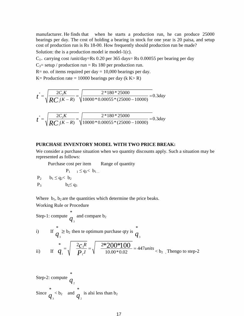
17
manufacturer. He finds that when he starts a production run, he can produce 25000
bearings per day. The cost of holding a bearing in stock for one year is 20 paisa, and setup
cost of production run is Rs 18-00. How frequently should production run be made?
Solution: the is a production model ie model-1(c).
C1= carrying cost /unit/day=Rs 0.20 per 365 days= Rs 0.00055 per bearing per day
C3= setup / production run = Rs 180 per production run.
R= no. of items required per day = 10,000 bearings per day.
K= Production rate = 10000 bearings per day (k K> R)
* 3
1
2 2*180 * 250000.3
( ) 10000 *0.00055* (25000 10000)
C Kday
K Rt
RC
* 3
1
2 2*180 * 250000.3
( ) 10000 *0.00055* (25000 10000)
C Kday
K Rt
RC
PURCHASE INVENTORY MODEL WITH TWO PRICE BREAK:
We consider a purchase situation when wo quantity discounts apply. Such a situation may be
represented as follows:
Purchase cost per item Range of quantity
P1 1 ≤ q1< b1…
P2 b1 ≤ q2< b2
P3 b2≤ q3
Where b1, b2 are the quantities which determine the price beaks.
Working Rule or Procedure
Step-1: compute 3
*
q and compare b2
i) If 3
*
q ≥ b2 then te optimum purchase qty is 3
*
q
ii) If 3
1 1
2 2*447
. 10.00*0.02
*200*100Runits
I
cq P
< b2 , Thengo to step-2
Step-2: compute 2
*
q
Since 3
*
q < b2 and 2
*
q is alsi less than b2

17
thus there are only two possibilities when 3
*
q < b2 , ie
either 2
*
q ≥ b1 or
2
*
q b1
(i) if
2
*
q < b2 but 2
*
q ≥ b1 then proceedas in the case of one price beak only.
that is compare the costs C(2
*
q ) and C(b2) to obtain the optimum purchase quantity. The
quantity with lower cost will naturally be the optimum
iii) If 2
*
q (b2 and b1 both ) then go to step-3.
Step-3: If 2
*
q (b2 and b1 both ) then compute 1
*
q which will satisfy the inequality
1
*
q<b1
in this case compare the costs C(1
*
q) with C(b1) and C(b2) both to determine the optimum
purchase quantity.
Problem-1: Find the optimal order quantity for a product for which the price breaks are as
follows:
Quantity 0 ≤ q1< 500 500 ≤ q2< 750 750 ≤ q3
Unit cost (Rs) 10.00 9.25 8.75
The monthly demand for a product is 200 units, the cost of storage is 2% of the unit cost
and the cost of ordering is Rs 350.
Soln: R = 200 units / month C3= Rs 350 I = 0.02
P1 = Rs 10.00 P2 = 9.25 P3 = 8.75
b1 = 500, b2= 750
step-1 : compute 3
*
q and obtain 3
3 3
2 2*894
. 8.75*0.02
*350*200R
I
cq P
since 3
*
q >b2 ie 894 > 750, therefore the optimum purchase quantitywill be 3
*
q = 894
Example-2: Find q*
, where R - 200 items/monthC3= 100/-, I = 0.09 ( ie 2% of the unit
cost) and for

17
P1 = Rs 10.00 for 0 ≤ q1< 500
P2= Rs 9.25 for 500 ≤ q2< 750
P3= Rs 8.75 for 500≤ q3
Soln: compute 3
*
q and obtain
*3
13
2 2478
. 8.75*0.02
*200*100R
I
cqP
Since 3
*
q < b2
ie ( 478 < 500 ) so compute 2
*
q
3
2
2 2*465
2. 9.75*0.02
*200*100R
I
cq
Since 2
*
q < b1
ie ( 465< 500 ) so compute *
1q
3
12
2 2*268
25.000*0.10.
100,00,0000.9901
cos 100,00,000 1,00,000
*500*180R
I
Lossorprofit
Lossorprofit tofspare
cq p
Comput C( 1
*
q ) = C (447) = 2090.42
C(b1) = C (500)= = 1937.25
C(b2) = C)750) = = 1843.29 minimum
Therefore C(750) < C(500) < C (*
1q = 447)
The optimum purchase quantity 1
*
q = 750
Example-3: if b1=400 ( instead of 500)
b2= 3000 ( instead of 750)
Find q* , where R - 200 items/monthC3= 100/-, I = 0.09 ( ie 2% of the unit cost) and for

18
P1 = Rs 10.00 for 0 ≤ q1< 400
P2 = Rs 9.25 for 400 ≤ q2< 3000
P3 = Rs 8.75 for 3000≤ q3
Solution: Compute 3
*
q and obtain
*3
13
2 2478
. 8.75*0.02
*200*100R
I
cqP
units…
Since 3
*
q < b2
ie ( 478 < 30000 ) so compute 2
*
q
3
2
2 2*465
2. 9.75*0.02
*200*100R
I
cq
Since 2
*
q < 465which falls with in the range ( 400 ≤ q2< 3000 O
There is no need to calculate *
1q
Rather compare only C(q2) = C(465) = = Rs1937
ie ( 465< 500 ) so compute *
1q
C (3000)= =Rs 2020.17
Since (2
*
q ) < C (3000), the most economical purchase quantity is 2
*
q = 465
Example-4:
if b1 = 1500 ( instead of7 50)
P2= 9.00 ( instead of 8.75)
R = 200 items/monthC3= 100/-, I = 0.02 ( ie 2% of the unit cost) and for
P1 = Rs 10.00 for 0 ≤ q1<500
P2 = Rs 9.25 for 500 ≤ q2<1500
P3 = Rs 9.00 for 1500≤ q
Soln: compute 3
*
q and obtain
.
3
3
2 2*471
2. 9.00 * 0.02
*200*100Runit
I
cq which is
less than 1500

18
Since 3
*
q < b2
ie ( 471 <1500 ) so compute 2
*
q
2
*
q3
2 21 465
2. 9.25*0.02
*200*100R
I
c
Since 2
*
q < 465which < 500 , so compute *
1q
3
1 1
2 2*447
. 10.00*0.02
*200*100Runits
I
cq P
Compare C(1500), C(500) and C(*
1q =447)
C(1500) = = Rs 1949.33
C(500)= = Rs 1937.25 minimum
C(*
1q =447) = =Rs 2090.42
Hence in this situation the optimum purchase quantity is q*= 500
Problem-5:
if b1 = 3000 ( instead of 500)
and b2= 5000 ( instead of 750)
P2= 9.00 ( instead of 8.75)
R = 200 items/monthC3= 100/-, I = 0.02 ( ie 2% of the unit cost) and for
P1 = Rs 10.00 for 0 ≤ q1< 3000
P2 = Rs 9.25 for 3000 ≤ q2< 5000
P3 = Rs 8.75 for 1500≤ q3
Soln: compute 3
*
q and obtain 3
3
2 2*478
2. 8.75* 0.02
*200*100Runit
I
cq
.
which is
less than 1500
Since 3
*
q < b2 ,
3
*
q < 500
ie ( 471 < 500 ) so compute 2
*
q

18
2
*
q3
2 2465
2. 9.25*0.02
*200*100R
I
c units
Since 2
*
q < 465which < 3000 , so compute *
1q
3
1 1
2 2*447
. 10.00*0.02
*200*100Runits
I
cq P
Compare C(3000), C(5000) and C(*
1q =447
C(*
1q =447) = =Rs 2092.42 minimum
C(3000) = = Rs 2135.17
C(5000)= = Rs 2192.50
Hence in this situation the optimum purchase quantity is q*= 447
PURCHASE INVENTORY MODEL WITH NUMBER OF PRICE BEAKS
Problem- :The annual demand for a product is 500 units. The cost of storage per unit per
year is 10% of the unit cost. The ordering cost is Rs 180 for each order. The unit cost
depends upon the amount ordered. The range of amount ordered and the unit cost price are
as follows:
Range of amount ordered 0 ≤ q1< 500 500 ≤ q2< 1500 1500 ≤ q3< 3000, 3000 ≤
q4
Unit cost (Rs) 25.0024.8024.60 244.40
Find the optimal order quantity?
Obviously this problem has three price beaks only
Soln: compute 4
*
q and obtain4
*
q = 32 2
2722. 24.40*0.10
*500*180R
I
c , 4
*
q
Since 3
4
*( 272) ( 3000)bq
4
*
q = 272 is not optimal order quantity, so proceed to compute 3
*
q as
3
*
q 270 units does not lie in the range 1500 ≤ q3< 3000, so 3
*
q = 270 is not the optimal
3
3
2 2*270
2. 24.600 * 0.10
*500*180R
I
cq

18
order qty,
So next compute 2
*
q , 3
22
2 2*269
24.80* 0.10.
*500*180R
I
cq p
which is less than b2,
b1 both . Therefore as per rulecompute
ie ( 471 < 500 ) so compute 1
*
q and compare the cost C(*
1q )
with C( b2) and C (b1)
Since 2
*
q < 465which < 3000 , so compute *
1q
3
12
2 2*268
25.000 * 0.10.
*500*180R
I
cq p
Compare C(3000), C(5000) and C(*
1q = 268)
* *
*1 1 1 1
1
1( ) *
3 2*
RC R Iq p p qC
q
) =
* *
*1 1 1 1
1
1( ) *
3 2*
RC R Iq p p qC
q
C(*
1q = 268) =
500 1500* 25 *0.10* 25* 268 13,170.82
2*180
268Rs minimum
1 12 2
1
1( ) *
3 2*
RC R Ip pb bC
b
* 500 1( ) 500* 24.80 *0.10* 24.80*500 13200.00
2500 *180
500C Rs
*2 23 3
2
1( ) *
3 2
500 1(1500) 500* 24.60 *0.10* 24.60*1500 14205.00
2
500 1(3000) 500* 24.40 *0.10* 24.40*3000 30 12200 3660 15890
2
*
*1801500
*1803000
RC R I
C
C
p pb bCb

18
Since C (1
*
q ) < C(b1) < C( b2)
C(268) < C (500) < C(1500)
1
*
q = 268 units is the optimum order quantity
STOCHASTIC INVENTORY MODELS
Instantaneous demand , no setup cost model
VI (a): discrete case
Find the optimum order level Z which minimizes the total expected cost under the following
assumptions:
t= constant interval between orders ( t may be considered as unity, e.g. daily,
weekly, monthly etc,)
Z= the stock ( in discrete units) at the beginning of each day
d= is the estimated (random) demand at discontinues rate with probability P(d). ie
demand d arises at each interval with probability P(d).
C1= holding cost per item per ‘t’ time unit
C2= shortage cost per item per t time nit.
Lead time is zero.
Demand is instantaneous.
In this model with instantaneous demand, it is assumed that the total demand is filled-up at
the beginning of the period. Thus depending on the amount d demanded, the inventory
position just after the demand occurs may beeither positive (surplus)or negative (shortage)
News paper problem: a newspaper boy buys papers for Rs 2.60 each and sells them for Rs
3.60 each. He cannot return unused news papers. Daily demand has the following
distribution.
No. of
customers
23 24 25 26 27 28 29 30 31 32
Probability 0.01 0.03 0.06 0.10 0.20 0.25 0.15 0.10 0.05 0.05
if each day’s demand is independent of the previous day’s , how many papers should he
order each day.
Solution:
Z= no of news papers ordered per day
D = the demand ie demand that could be sold per day, if z ≥ d
P(d)= the probability that the demand will be equal to ‘d’ on a randomly selected day.
c1 = cost per news paper
c2 = selling price oer year
if d exceeds ie d>= Z
profit = c2 – c1 and no paper will be left unsold

18
demand d < Z
Profit becomes = (c2 - C1 ) d + (Z-d) c1
No. of
customers
23 24 25 26 27 28 29 30 31 32
Probability 0.01 0.03 0.06 0.10 0.20 0.25 0.15 0.10 0.05 0.05
cum
probability
0.01 0.040. 0.10 0.20 0.40 0.65 0.80 0.90 0.95 0.95
C1 = holding cost / paper/day
C2= shortage cost /paper
2
23
2
( )
1
Z
dp d c
cc
But C1 = c1 = 2.60
C2= c2 – c1= 3.60-2.60 = 1.00
Hence 2
1 2
2.60 2.60
1.00 2.60 3.60
cc c
0.2777
23( ) 0.2777
Z
dp d
gives value of Z= 27 through above table.
Problem-2: Some of the spare parts of Ship costs Rs 1,00,000 each. These spare parts can
only be ordered together with the ship. If not ordered at the time , when the ship is
constructed, these parts cannot be made available on need. Suppose that a loss of Rs 100,
00,000 is suffered for each spare part is needed, when none is available in the stock. Further
, suppose that probabilities that spare parts will be needed as replacement during the life-
term of the class of the ship discussed are
Spares
required
0 1 2 3 4 5 or more
Probability 0.9488 0..0400 0.0100 0.0010 0.0002 0.0000
How many spares parts should be procured?
Solution:
C1 = c1 = 1,00,000
C2= c2= shortage cost = Rs 100,00,000
Spares required 0 1 2 3 4 5 or more

18
Probability 0.9488 0..0400 0.0100 0.0010 0.0002 0.0000
cum. prob 0.9488 0.9888 0.9988 09998 1.0000 1.0000
2
2
100000 100,00,000 100,00,000. 0.9901
10,00,000 1,00,00 100,00,000 1,00,000 101,00,0001
ccc
2
23
2
( )
1
Z
dp d c
cc
= 100,00,000
0.9901cos 100,00,000 1,00,000
Lossorprofit
Lossorprofit tofspare
Which gives Z = 2
Model VI(b): CONTINUOUS CASE:
Instantaneous demand, setup cost zero, stock levels continuous, lead time zero
This model is same as Model VI(a), except that the stock levels are now assumed to be
continuous (rather than discrete ) quantities. So instead of probability P(d), we shall have
f(x)dx, where f(x) is the probability density function.
∫ 𝑓(𝑥)𝑑𝑥𝑥2
𝑥1= The probability of an order with in the range x1 to x2
now , the cost equation fr this model will be similar to model VI(a). only p(d) is replaced by
f(x)dx and the ∑ is replaced by the sign of integration
(∫). 𝑡ℎ𝑒𝑛 𝑡ℎ𝑒 𝑐𝑜𝑠𝑡 𝑒𝑞𝑢𝑎𝑡𝑖𝑜𝑛 𝑜𝑟 𝑡ℎ𝑖𝑠 𝑚𝑜𝑑𝑒𝑙 𝑏𝑒𝑐𝑜𝑚𝑒𝑠:
C(Z) =C1∫ (𝑧 − 𝑥)𝑓(𝑥)𝑑𝑥 𝑧
0+ C2∫ (𝑥 − 𝑍)𝑓(𝑥)𝑑𝑥
∞
𝑥 ------ eqn-1
Hence we can get optimum value of z satisfying eqation -1 for which the total expected cost
C is minimum.
∫ (𝑧 − 𝑥)𝑓(𝑥)𝑑𝑥 𝑧
0= C2/(C1 +C2) =
𝐶2
𝐶1+𝐶2
Problem-3: A backing company sells cake by the kg weight. It makes a profit of Rs 5.00 a kg
on each kg sold on the day it is baked. It disposes of all cake not sold on the date of it is
baked at a loss of Rs1.20 a kg. If demand is known to be rectangular between 2000 and 3000
kg. determine the optimal daily amount baked.
Soln: let
C1= the carrying cost unsold cake if not sold on the day ogf baking = Rs 1.20
C2 = the profit per kg = Rs 5
23( ) 0.9901
Z
dp d

18
x = the demand which is continuous with probability density f(x).
∫ 𝑓(𝑥)𝑑𝑥 𝑥2
𝑋1= the probability of an order with in the range x1 to x2
Z= the stock level
∫ 𝑓(𝑥)𝑑𝑥 𝑧
𝑥1=
𝐶2
𝐶1+𝐶2 -------- eqn-2
x1= 2000, x2= 3000
f(x) = 1
𝑥2−𝑥1 =
1
3000−2000=
1
1000
Substituting the values in the equation-2 we get
∫ (𝟏
𝟏𝟎𝟎𝟎)𝒅𝒙
𝒛
𝟐𝟎𝟎𝒐=
𝟓.𝟎𝟎
𝟏.𝟐𝟎+𝟓.𝟎𝟎 = 0.807
[1/1000 x] = 0.807
Z= 2807.
Problem-4 An ice cream company sells one of its types of ice cream by weight. If the
product is not sold on the day it is prepared, it can be sold at a loss of 50 paise per kg. but
there is an unlimited market for one day old ice-cream . on the other hand, the company
makes a profit of Rs 3.20 on every kg of ice-cream sold on the day it is prepared. Past daily
orders form a distribution with f(x) = 0.02 – 0.002x, 0 ≤ x ≤100. How many Kg of ice-
cream should the ccompany prepare every day.
Here C1 = bear 50 paise for every kg unsold= Rs 0.50
C2= profit per kg sold= Rs 3.20
f(x) = 0.02 – 0.002 x
directly using the result
∫ 𝑓(𝑥)𝑑𝑥 𝑧
0=
𝐶2
𝐶1+𝐶2 -------- eqn-2
∫ (0.02 − 0.002𝑥)𝑑𝑥 𝑧
0=
𝐶2
𝐶1+𝐶2 = 3.20
3.20
0.50+3.20---= 0.865----- eqn-2
[0.02x – 0.002x2 ] limits 0and Z
Z= 63.2 kgs
Model-VI(c) : Reorder lead time prescribed
It is similar to VI(a), with one important exception, that the re-order lead time is to be taken
into consideration . in other words, the time between placing an order and receiving the
goods is significant.
n= no. of order cycle periods in the reorder lead time
Z0 = the tock level at the end of the period preceding placing of order.
Let q1 q2 q3q4, -, -, -, -, qn-1 quantities already ordered and due to be received on the 1st, 2
nd,
3rd
, ---- and (n-1) th days.
F(x1
) = f(x1 + x2 + x3 + …………+ xn) wherex1
is the demand during lead time.

18
Our problem is to find the value of quantity qn in order to minimize the total expected cost of
the nth order cycle time. The opimumm value of Z1
is that value which satisfies the equation.
∫ 𝑓(𝑥)𝑑𝑥
𝑧
0
= 𝐶2
𝐶1 + 𝐶2
After the optimum value of z1
or Z*
is obtained , we can easily find the optimum value of qn
by using relationship.
qn*
= Z* -
[ Z0 + ∑ 𝑞𝑖𝑛−1𝑖=1 ]
Problem: A shop owner places orders daiy for goods which will be delivered 7 days latr (ie
the reorder lead time is 7 days). On certain day, the owner has 10 items in stock. Further
more on the 6 previous days, he has already placed orders, for the delivery of 2, 4, 1, 10, 11
and 5 items in that order over each of the next 6 days. To facilitate computations, we shall
assume C1= Rs 0.15 and C2= Rs 0.95 and the distribution requirement over a 7 day period
(x1) is f(x
1) = 0.02 – 0.0002 x
1.
how many items should be ordered for the 7th
day hence?
Soln: Substituting the values of C1 and C2 and f(x1) in the result.
∫ 𝑓(𝑥)𝑑𝑥
𝑧
0
= 𝐶2
𝐶1 + 𝐶2
∫ (0.02 − 0.0002𝑥)𝑑𝑥𝑧
0=
0.95
0.15+0.95= 0.8636
[0.02x – 0.ooo2. x/2 ] = 0.8636
Z2
– 0.02 Z + 0.8636 = 0
Z2
- 200 Z + 8600 = 0
Solving this quadratic equation we approximately get
Z1
= 63 or 136
Since Z1= Z0+ ∑ 𝑞𝑖6
𝑖=1` + q7
we have 63= 10 + ( 2 + 4+ 1 + 10 +11+ 5 ) + q7
q7 = 63-10-33 = 20 items
the optimum order quantity is 20 items.
UNIFORM DEMAND, NO SETUP COST, MODEL:
Under this probabilistic model, the type of problem s similar to model VI. Except, that with
drawals from stocks are continuous ( rather than instantaneous) and the rate of with drawl is
assumed to be virtually constant.
Model VII(a): continuous version
To find the optimum order level so as to minimize the total expected cost where
t is the scheduling period which is a prescribed constant
Z is the stock level to which the stock is raised at the end of every period t.

18
f(x) is the probability density function for demand x, whch is known
C1 = is the carrying cost per quantity unit per unit time
C2 is the shortage cost per quantity unit per unit time
Production is instantaneous
Lead time is zero
The demand rate in a period t is constant.
In this case , demand occurs uniformly rather than instantaneously during period t, as shown
in figures
∫ 𝑓(𝑥)𝑑𝑥 𝑧
0+ ∫
𝑓(𝑥)𝑑𝑥
𝑥
∞
𝑧=
𝐶2
𝐶1+𝐶2
Cost is minimum for the optimum value of Z given by above equation.
UNIT-V: WAITING LINES AND SIMULATION
In this we will discuss on following concepts
Queuing Theory Introduction
MIM/1 Queuing Model
Introduction In everyday life, it is seen that a number of people arrive at a
cinematicketwindow.Ifthepeoplearrive“toofrequently”they will have to wait for getting their tickets or sometimes do
without it. Under such circumstances, the only alternative is to form a queue, called the waiting line, in order to
maintain a proper discipline. Occasionally, it also happens that the person issuing tickets will have to wait, (i.e.
remains idle), until additional people arrive. Here the arriving people are called the customers
andthepersonissuingtheticketsiscalledaserver.
Another example is represented by letters arriving at a typist’s desk. Again, the letters represent the customers and the
typist represents the server. A third example is illustrated by a machine breakdown situation. A broken machine
represents a customer callingfortheserviceofarepair
man.Theseexamplesshowthat the term customer may be interpreted in various numbers of
ways.Itisalsonoticedthataservicemaybeperformedeitherbymovingtheservertothecustomerorthecustomer totheserver.
Thus, it is concluded that waiting lines are not only the lines of human beings but also the aero planes seeking to land
at busy airport, ships to be unloaded, machine parts to be assembled,
carswaitingfortrafficlightstoturngreen,customerswaitingfor attention in a shop or supermarket, calls arriving at a
telephone switch-board, jobs waiting for processing by a computer, or anything else that require work done on and for
it are also the examplesofcostlyandcriticaldelaysituations.Further,itisalso observed that arriving units may form one
line and be serviced through only one station ( doctor’s clinic),mayform one line and be served through several stations
(as in a barber shop), may form several lines and be served through as many stations {e.g. at check out counters of
supermarket).
Servers may be in parallel or in series. When in parallel, he arriving customers may form a single queue as shown in
Fig. Or individual queues in front of each server as is common in big post-offices. Service times may be constant or
variable and customers may be served singly or in batches (like passengers boarding a bus).

19
Fig (a). Queuing system with single queue and single service station..
Fig. (b). Queuing system with single queue and several service stations.
Fig. (c) Queuing system with several queues and several queues
Fig.illustrates how a machine shop may be thought of as a system of queues forming in front of a number of service
centers, the arrows between the centers indicating possible routesforjobsprocessedintheshop.Arrivalsataservicecentre are
either new jobs coming into the system or jobs, partially processed, from some other service centre. Departures from a
servicecentremaybecomethearrivalsatanotherservicecentre or may leave the system entirely, when processing on these
items iscomplete.
Queuing theory is concerned with the statistical description of the behavior of queues with finding, e.g., the probability
distribution of the number in the queue from which the mean and variance of queue length and the probability distribution
ofwaitingtimeforacustomer,orthedistributionofaserver’s busy periods can be found. In operational researchproblems
Involving queues, Investigators must measure the existing
systemtomakeanobjectiveassessmentofitscharacteristicsandmustdeterminehowchangesmaybemadetothesystem,whateffects
ofvariouskindsofchangesinthesystem’scharacteristics would be, and whether, in the light of the costs incurred in the
systems, changes should be made to it. A model of the queuingsystemunderstudymustbeconstructedinthiskindof analysis
and the results of queuing theory are required to obtain the characteristics of the model and to assess the effects of changes,
such as the addition of an extra server or a reduction in mean service time.
Perhaps the most important general fact emerging from the theory is that the degree of congestion in a queuing system
(measured by mean wait in the queue or mean queue length) is very much dependent on the amount of irregularity in the
system. Thus congestion depends not just on mean rates at which customers arrive and are served and may be reduced
without altering mean rates by regularizing arrivals or service times, or both where this can be achieved.
Meaning of a Queuing Model A Queuing Model is a suitable model to represent a service- oriented problem where customers arrive randomly to receive
some service, the service time being also a random variable.
Objective of a Queuing Model The objective of a queuing model is to find out the optimum service rate and the number of servers so that the average cost

19
of being in queuing system and the cost of service are minimized.
The queuing problem is identified by the presence of a group ofcustomerswhoarriverandomlytoreceivesomeservice.
Thecustomeruponarrivalmaybeservedimmediatelyorifwillingmayhavetowaituntiltheserverisfree.
Application of a QueuingModel The queuing models are basically relevant to service oriented organizations and suggest ways and means to improve the
efficiency of the service. This model can be applied in the field of business (banks, booking counters), industries (servicing
of machines), government (railway or post-office counters), transportation (air port, harbor) and everyday life (elevators,
restaurants, doctor’s clinic).
Relationship between Service and Cost Improvement of service level is always possible by increasing the number of employees. Apart from increasing the cost an
immediate consequence of such a step unutilized or idle time of the servers. In addition, it is unrealistic to assume that a
large-scale increase in staff is possible in an organization.
Queuing methodology indicates the optimal usage of existing manpower and other resources to improve the service. It can
also indicate the cost implication if the existing service facility has to be improved by adding more servers.
The relationship between queuing and service rates can be diagrammatically illustrated using the cost curves as shown in
following figure.
At a slow service rate, queues build up and the cost of queuing increases.Anidealserviceunitwill minimize
theoperatingcost of the entiresystem.
Arrival The statistical pattern of the arrival can be indicated -through -
i. the probability distribution of the number of arrivals in a specific period of time,or
ii. the probability distribution of the time between two successive arrival (known as
interarrival time) number of arrivals is a discrete variable whereas the interarrival times
arecontinuousrandomandvariable.Aremarkableresulting this context is that if the number
of arrivals follows a ‘Poisson Distribution’, the corresponding interarrival time follows
an ‘Exponential Distribution’. This property is frequently used to derive elegant results
on queuing problems.
Service The time taken by a server to complete service is known as service time. The service time is a statistical
variable and can be studied either as the number of services completed in a given period of time or the
time taken to complete the service. The data on actual service time should be analyzed to find out the
probability distribution of service time. The number of
servicescompletesdiscreterandomvariablewhiletheservice time is a continuous randomvariable.
Server A server is a person or a mechanism through which service is
offered.Theservicemaybeofferedthroughasingleserversuch as a ticket counter or through several channels
such as a train arriving in a station with several platforms. Sometimes the service is to be carried out
sequentially through several phases known as multiphase service. In government, the papers move through a
number of phases in terms of official hierarchy till theyarriveattheappropriatelevelwhereadecisioncanbetaken.
Time Spent in the Queueing System The time spent by a customer in a queuing system is the sum of waiting time before service and the service

19
time. The waiting time of a customer is the time spent by a customer in a queuing system before the service
starts. The probability distribution of waiting time depends upon the probability distribution of interarrival
time and service time.
Queue Discipline The queue discipline indicates the order in which members of the queue are selected for service. It is most
frequently assumed that the customers are served on a first come first serve basis. This is commonly referred
to as FIFO (first in, first out) system. Occasionally, a certain group of customers receive priority in service
over others even if they arrive late. This is commonly referred to as priority queue. The queue discipline
does not always take into account the order of arrival. Theserver chooses one of the customers to offer
service at random. Such a system is known as service in random order (SIRO).
While allotting an item with high demand and limited
supplysuchasatestmatchticketorshareofapubliclimitedcompany, SIRO system is the only possible way of
offering service when it is not possible to identify the order ofarrival.
Kendall’s Notation Kendall’s Notation is a system of notation according to which the various characteristics of a queuing model
are identified. Kendall (Kendall, 1951) has introduced a set of notations, which have become standard in the
literature of queuing models. A general queuing system is denoted by (a/b/c) :(d/e) where
a = probability distribution of the inter arrival time. b = probability distribution of the service time.
c = number of servers in the system.
d = maximum number of customers allowed in the system. e = queue discipline
In addition, the size of the population is important for certain types of queuing problem although not
explicitly mentioned in the Kendall’s notation. Traditionally, the exponential distribu- tion in queuing
problems is denoted by M. Thus (MIMI!): (¥/ FIFO) indicates a queuing system when the inter arrival times
and service times are exponentially distributed having one server in the system with first in first out
discipline and the number of customers allowed in the system can be infinite.
State of Queueing System The transient state of a queuing system is the state where the probability of the number of customers in the
system depends upon time. The steady state of a queuing system is the state where the probability of the
number of customers in the system is independent oft.
Let Pn (t) indicate the probability of having n customers in the system at time t. Then if Pn(t) depends upon
t, the queuing system is said to be in the transient state. After the queuing system has become operative for a
considerable period of time, the probability Pn(t) may become independent of t. The probabilities are then
known as steady state probabilities
Poisson Process When the number of arrivals in a time interval of length t follows a Poisson distribution with parameter (At),
which is the product of the arrival rate (A-)and the length of the interval t, the arrivals are said to follow a
poison process.
Relationship Between Poisson Process And Exponential
Probability Distribution
1. Ifthenumberofarrivalsinatimeintervaloflength(t)for How’s a Poisson Process,
then corresponding inter arrival time follows an ‘ExponentialDistribution’.
2. If the interarrival times are independently, identically distributed random
variables with an exponential probability distribution, then the number of
arrivals in a timeintervaloflength(t)followsaPoisson processwith arrival rate
identical with parameter of the Exponential Distribution.
MIM/1 Queuing Model
The M/M/1 queuing model is a queuing model where thearrivals follows
aPoissonprocess,servicetimesareexponentially distributed and there is oneserver.

19

19
The assumption of M/M/1 queuing model are as follows:
1. The number of customers arriving in a time interval t follows a Poisson Process with parameter
A.
2. Theintervalbetweenanytwosuccessivearrivalsis exponentially distributed with parameterA.
3. Thetimetakentocompleteasingle service isexponentially distributed with parameter1.1
4. The number of server isone.
5. Althoughnotexplicitlystatedboththepopulationandthequeue size canbeinfinity.
6. The order of service is assumed to beFIFO.
7.
The time spent by a customer in the system taking into account both waiting and service time is an exponential
distributionwithparameter the probability distribution oftheWaitingtimebeforservicecanalsobederivedinanidentical
manner. The expected number of customers in the system is given by–
Optimum Value of Service Rate
The study of queuing models helps us to find a cost model, which minimizes the sum of costs of service and of waiting
time per unit time. Generally, it is assumed that the cost of waiting is directly proportional to the total time that the customers
spend in the system, both waiting and in service. Theservicecanusuallybeascertainedfromthevariousavailable records.

19
Assuming a single server model with an arrival rate A and service rate 11and that the service rate 11is controllable, optimum
value of service rate 11can be determined as follows:
Let
Fundamental Process Component Elements of a Queuing The fundamental components of a queuing process are listed below:
1. The input process or thearrivals
2. Servicemechanism
3. Queuediscipline
We now give a brief description of each of the above components:
1. TheInputProcess:Customersarriveataservicestationfor service. They do not come at regular
intervals but arrivals into the system occur according to some chance mechanism. Often an
arrival occurs at random and is independent of what has previously occurred. Customers
may arrive for service individually or in groups. Single arrivals are illustrated by customers
visiting a bank. On the other hand, families visiting a restaurant, is an example of bulk or
group arrival. Arrivals may occur at a constant rate
ormaybeinaccordancewithsomeprobabilitydistribution such as Poisson distribution or
normal distribution etc. Frequently the population of the units or customers requiring
service may be infinite e.g. passengers waiting across the booking counters but there are
situations where the population may be limited such as the number of particular equipment
breaking down and requiring service from the factory’s maintenance crew. Thus, in
connection with the input process, the following information is usually called for and is
consideredrelevant:
i. Arrivaldistribution
ii. inter-arrivaldistribution
iii. meanarrivalrate;(ortheaveragenumberofcustomers arriving in one unit of time)and
iv. mean time betweenarrivals.
2. ServiceMechanism:Analogoustotheinputprocess,there are probability distribution of
service times and number ofcustomersservedinaninterval.Servicetimecaneither be fixed
(as in the case of a vending machine) or distributed in accordance with someprobability distribution. Service facilities can be anyone of the following types:

19
i. Single channel facility or one queue-one service station facility – This means that
there is only one queue in whichthecustomerwaitstilltheservicepointisready to take
him for servicing. A library counter is an example ofthis.
ii. One queue-several service station facilities:Inthiscase customers wait in a single
queue until one of the service stations is ready to take them for servicing.
Bookingataservicestationthathasseveralmechanics each handling one vehicle,
illustrates this type of model.
iii. Several queues-one service stations - In such a
situation,thereareseveralqueuesandthecustomercan join anyone of these but the service
station is onlyone.
iv. Multi-channel facility - In this model, each of the
servershasadifferentqueue.Differentcashcountersin an Electricity Board Office where
the customers can make payment in respect of their electricity bills provides an
example of this model. Booking counters at railway station provide anotherexample.
v. Multi-stage multi-channel facilities - In this case,
customersrequireseveraltypesofserviceanddifferent service stations are there. Each
station provides a specialized service and the customer passes through each of the
several stations before leaving thesystem.
For example, machining of a certain steel item may consist of cutting, turning, knurling, drilling, grinding and packaging
etc., each of which is performed by a single server in a series.
In connection with the service mechanism the following information is often obtained from the point of view of the
queuing theory:
i. Distribution of number of customersserviced
ii. Distribution of time taken to servicecustomers
iii. Average number of customers being serviced in oneunit of time at a servicestation.
iv. Averagetimetakento serviceacustomer.
3. Queue Discipline: Queue discipline may refer to many
things.Oneofsuchthingsistheorderinwhichtheservice station selects the next customer
from the waiting line to beserved.Inthiscontext,queuedisciplinemaybelikefirst in first out
or last in first out or may be on the basis of
certainothercriteria.Forexample,itmayberandomwhen a teacher picks up the students for
recitation. Sometimes thecustomermaybegivenaprioritybasisforserviceon the basis of
ladies first. Another aspect of queue discipline is whether a customer in a queue can
move to a shorter queue in the multi-channel system. Queue discipline also refers to the
manner in which the customers form into queue and the manner in which they behave in
the queue. For example, a customer may get impatient and leave the queue.
Conditions For Single ChannelQueuingModel

19
Thesinglechannelqueuingmodelcanbefittedinsituations where the following seven
conditions arefulfilled:
1. The number of arrivals per unit of time is described by Poisson distribution. The
mean arrival rate is denotedby
2. Theservicetimehasexponentialdistribution.Theaverage service rate is denotedby
3. Arrivals are from infinitepopulation.
4. ThequeuedisciplineisFIFO,thatis,thecustomersare served on a first come first
servebasis.
5. There is only a single servicestation.
6. Themeanarrival rate islessthanthemeanserviceratei.e.< 11.
7. Thewaitingspaceavailableforcustomersinthequeueis infinite. .
Limitations of Single Channel Queuing Model
The single channel queuing model referred above is the simplest model, which is based on the above-mentioned
assumptions.
However, in reality, there are several limitations of this model in
Itsapplications.Oneobviouslimitationisthe possibilitythat the waiting space may in fact be limited. Another possibilityis
Thatarrivalrateisstatedependent.Thatis,potentialcustomers are discouraged from entering the queue if they observe
along lineatthetimetheyarrive.Anotherpracticallimitationofthemodelisthatthearrivalprocessisnotstationary.Itisquite
possible that the service station would experience peakperiodsand slack periods during which the arrival rate is
higher and
lowerrespectivelythantheoverallaverage.Thesecouldoccuratparticulartimesduringadayoraweekorparticularweeksdurin
gayear.Thereisnotagreatdealonecandotoaccountfor stationary without complicating the mathematics
enormously. The population of customers served may be finite, the queue discipline may not be first come first serve.
In general, the validity of these models depends on stringent assumptionsthatareoftenunrealisticinpractice.
Evenwhenthemodelassumptionsarerealistic,thereisanotherlimitation of queuing theory that is often
overlooked.Queuingmodels give steady state solution, that is, the models tell us what will happen after queuing
system has been in operation long enough to eliminate the effects of starting with an emptyqueue at the beginning
ofeach business day. In someapplications, the queuing system never reaches a steady state, sothemodel solutions are
of little value.
Model-1: Model (M/M/1): (∞/𝐹𝐶𝐹𝑆)Single channel-poisson arrival with exponential service – infinite population
Model.
Problem-1: An airport runway for arrivals only. Arriving aircraft join a single queue fr rthe runway. Exponentially
distributed service time with a rate 27 arrivals/hour. arrival rate 20 arrivals / hour. Find
a) Average number of customers in the system.
b) Average no. of customers in the queue.
c) Average time a customer spends in the system.
d) Average time a customer spends in the queue.
𝜇𝜆
λ = mean arrival rate = 20 arrivals /hour

19
𝜇= Mean service rate = 27 nos /hour
a)Average number of customers in the system.= Ls= 𝛌
(𝜇−𝜆)=
20
(27−20)= 20/7=2.9 aircrafts
b)Average no. of customers in the queue. Lq= 𝛌∗ 𝐋𝐬
𝜇=(
𝜆
𝜇) ∗
𝛌
(𝜇−𝜆)= (
20
7) ∗
20
(27−20)= 2.1 aircrafts
c)Average time a customer spends in the system.=Ws= 𝟏
(𝜇−𝜆)=
𝟏
(27−20)= 8.6 min
d)Average time a customer spends in the queue.= Wq= 𝜆
𝜇* (Ws) =
𝜆
𝜇*
𝟏
(𝜇−𝜆)=
1
(27−20)
20
27∗
1
(27−20)= 0.1058 hour= 6.3 minutes
Problem-2: suppose we are in holiday and the arrival rate increase 25 arrivals /hour. How will the quantities of
queuing system change.
λ = mean arrival rate = 25 arrivals /hour
𝜇= Mean service rate = 27 nos /hour
a) Average number of customers in the system.= Ls= 𝛌
(𝜇−𝜆)=
25
(27−25)= 12.5 air crafts
b)Average no. of customers in the queue.Lq= 𝛌∗ 𝐋𝐬
𝜇=(
𝜆
𝜇) ∗
𝛌
(𝜇−𝜆)= (
25
27) ∗
25
(27−25)= 11.6 aircrafts
c)Average time a customer spends in the system.=Ws= 𝟏
(𝜇−𝜆)=
𝟏
(27−25)= 1/5 hour= 30 min
b) Average time a customer spends in the queue.= Wq= 𝜆
𝜇* (Ws) =
𝜆
𝜇*
𝟏
(𝜇−𝜆)=
25
27∗
1
(27−25)= 0.1058 hour= 2.8 minutes
Problem-3: Suppose we have bad weather and the service rate decreases 𝜇 = 22 𝑎𝑟𝑟𝑖𝑣𝑎𝑙𝑠 𝑝𝑒𝑟 ℎ𝑜𝑢𝑟. how will the
quanties of queuing system changes.
𝜇= Mean service rate = 22 nos /hour
λ = mean arrival rate = 20 arrivals /hour
a) Average number of customers in the system.= Ls= 𝛌
(𝜇−𝜆)=
20
(22−20)= 10 air crafts
b)Average no. of customers in the queue.Lq= 𝛌∗ 𝐋𝐬
𝜇=(
𝜆
𝜇) ∗
𝛌
(𝜇−𝜆)= (
20
22) ∗
20
(22−20)= 9.1 aircrafts
c)Average time a customer spends in the system.=Ws= 𝟏
(𝜇−𝜆)=
𝟏
(22−20)= 1/2 hour= 30 min
b) Average time a customer spends in the queue.= Wq= 𝜆
𝜇* (Ws) =
𝜆
𝜇*
𝟏
(𝜇−𝜆)=
20
22∗
1
(22−20)= 10/22 hour= 27.27 minutes
e) Problem-4: A self-service store employees one cahier at its counter. None customers arrive at an average every 5
minutes while the cashier can serve 10 customers in 5 minutes. Assuming Poisson distribution for arrival rate and
exponential distribution for service rate. Find.

19
a) Average number of customers in the system.
b) Average no. of customers in the queue.
c) Average time a customer spends in the system.
d) Average time a customer spends in the queue.
Arrival rate = λ = 9/5 customers per minute= 1.8 customers/minute
service rate = 𝜇= 10/5 customers per minute= 2.0 customers/minute
a) Average number of customers in the system.= Ls= 𝛌
(𝜇−𝜆)=
1.8
(2.0−1.8)= 9 customers
b)Avg.no. of customers in the queue.Lq= 𝛌∗ 𝐋𝐬
𝜇=(
𝜆
𝜇) ∗
𝛌
(𝜇−𝜆)= (
1.8
2.0) ∗
1.8
(2.0−1.80)= 8.1 customers
c)Average time a customer spends in the system.=Ws= 𝟏
(𝜇−𝜆)=
𝟏
(2.0−1.80)= 5 minutes
b) Average time a customer spends in the queue.= Wq= 𝜆
𝜇* (Ws) =
𝜆
𝜇*
𝟏
(𝜇−𝜆)=
1.80
2.0∗
1
(2.0−1.8)= 4.5 minutes
Problem-5: At a certain petrol pump, customers arrive according to a poisson process with an average time of 5
minutes between arrivals. The service time is exponentially distributed with mean time of 2 minutes.on the basis of
this information. Find out
a) What would be the average que length? Lq
b) what would be the average no of customers in the queueing system Ls
c) What is the average time spent by a car in the petrol pump? Ws
d) What is the average waiting time of a car before receiving petrol Wq
e) Solution: ths is an M/M/! queueing model .
Average inter arrival time = 5 minutes
λ = mean arrival rate = 1/5 units/minutes =( 1/5 )*60 = 12 units/hour
average service time = 2 minutes
Mean service rate = 𝜇 = 1
2𝑛𝑜𝑠 𝑝𝑒𝑟 𝑚𝑖𝑛𝑢𝑡𝑒𝑠 =
1
2∗ 60 = 30
𝑢𝑛𝑖𝑡𝑠
ℎ𝑜𝑢𝑟
Since λ <𝜇
, the steady state solution exists.
Lq= Average queue length = 𝛌∗ 𝐋𝐬
𝜇=(
𝜆
𝜇) ∗
𝛌
(𝜇−𝜆)= (
12
30) ∗
12
(30−12)= 4/5 customers
Ls = average no of customers in the queue system= = 𝛌
(𝜇−𝜆)=
12
(30−12)= 2/3 customers
Average time spent in the petrol pump = Ws = = 𝟏
(𝜇−𝜆)=
𝟏
(30−12)= 1/18 hour= 3.33 minutes
c) Average waiting time of a c𝜆
𝜇*
𝟏
(𝜇−𝜆)= ar before receiving petrol = Wq=
𝜆
𝜇* (Ws) =
12
30*
𝟏
(30−12)= 1/45 hour = 1.33
minutes
Problem: 6 at a certain petrol pump , customers arrive according to a Poisson process with an average time of 55
minutes between arrivals. The service time is exponentially distribution with mean time of 2 minutes. Find
a) The average queue length ( Lq)
b) The average no. of customers in the queueing system ( Ls)

20
c) Average time spent a customer in a pertrol pump. (Ws)
d) Average time of a customer before receiving the service (Wq)
e) If the waiting time in queue is 4 min, a second pump will be considered. What should be the arrival rate for scond
pump.
Solution: this is an (M/M/1) : (∞! 𝐹𝐶𝐹𝑆) 𝑄𝑈𝐸𝑈𝐸 𝑀𝑂𝐷𝐸𝐿λμ
AVERAGE INTER ARRIVAL TIME = 1
λ= 5 MIN
λ = 1/5 nos per minute
= 12 nos / hour
μ = mean service rate = ½ nos per minutes
= ½ * 60 = 30 nos per hour
As λ < μ , the steady state solution exists.
a) Average length of Queue =
2 2
( ) 30(30 12)
4
15
12qL
λ
λnos
b) Average length of system 12
( ) (30 )
2
312sL
λ
λ nos
c) Average time spent in the petrol pump (system)= Ws=
( ) (30 12)
1 1 13.33min
18shourW
λ
d) Average waiting time of customer in queue ie before receiving the service = Wq=
1
( ) 30(30 1
11.33min
452)qhourW
λ
λ
Or
13.33 2 1.33min
sWq W
e) To open second pump Wq
1
11 4m
(
4
5) 1qhourW
λλ
1
1
1
15 30(30 )hour
λλ
160 /3 20 /
int 3min
nos hour
or erarrivaltime
λ
Model-II: Single channel Finite population model with Poisson arrivals and Exponential service times ( M:M:1) : (
N / FCFS)
In some cases , units arrive from a limited pool of potential customers. Once a unit joins the queue, there is one less
unit which could arrive , and therefore the probability of an arrival is lowered. When a unit is served, it rejoins the

20
pool of potential customers, and the probability of an arrival is there by increased. As a rule of thumb, if the
population is less than 40, the equations for finite population should be used. Although the concepts are same as
those for infinite populations, some of the terms are different and the equations required for analysis are different.
One distinct difference is that the probability of an arrival depends upon the number of potential customers available
to enter the system.
Let the total potential customers population is M,
The no. of customers already in the queuing system = n
Then any arrival must come from M-n number , that is not yet in the system.
1. The probability of an empty system = P0=
0
1
!( )
( )!
n Mn
n
M l
M n u
2. The probability of n customers in the system Pn= 0
0
!(
( )!!
(( )!
!(
( )!
)
)
)
n
n
n
n M
n
M
M nM
M nM
M n
P
λ
λ
λ
3) Ls = Expected number of customers in the system.
0
n M
nn
nP
4) Expected Number of customers in the queue= Lq= Ls -
λ=
0(1 )M P
λ
λ
Lq= Ls -
λ
Lq= 0
(1 )M P
λ
λ
Ws= sLλ
=
Wq= Ws - 1
=
sLλ
- 1
=
1 1( )*
q qL L
λ
λ λ λ
Problem-5: Amechanic repairs four machines. The mean time between service requirements is 5 hours for each machine
and forms an exponential m distribution. The mean repair time is 1 hour and also follows the same distribution pattern.
Machine downtime costs Rs 25 per hour and mechanic costs Rs55 per day.
i. Find the expected no. of operating machines
ii. Determine the expected down time cost per day.
iii. Would it be economical to engage two mechanics, each repairing only two machines.

20
Solution: This situation involves finite population
When mechanic serving 4 machines M = 4
Arrival rate = λ = 1/5 = 0.2
Service rate 𝜇 =1
1= 1
Let us find the probability of an empty system
P0=
0
1
!( )
( )!
n Mn
n
M l
M n u
= 4
0
1
4! 0.2( )
(4 )! 1
nn
n n
= 1 2 3 4
1
4! 4! 4! 4!1 ( ( ( (
3! (4 2)! (4 3)! (4 4)!0.2) 0.2) 0.2) 0.2)
=2 3 4
10.40
1 4*0.2 4*3( 4*3*2*( (4*3*2*1)(0.2) 0.2) 0.2)
a) Expected number of broke down machines in the system Ls=
Ls =
14 (1 0.4) 4 5*0.6 1
0.2
the expected number of operating machines in the system = 4-1 =3
b) Expected down time cost per day ( assuming an 8 hours per day)
= 8 * Expected number of broken down m/cs * Rs 25 per hour= 8*1*25 = Rs 200 per day
c) When there are two mechanics each serving two machines ie M=2
P0=
0
1
!( )
( )!
n Mn
n
M l
M n u
= 2
0
1
2! 0.2( )
(2 )! 1
nn
n n
=
1 2 1 2
1 1
2! 2! 2! 2! 2! 2!( ( ( (
2! (1)! 2! (1)!
1 10.68
1 2*0.2 2*0.04 1.48
0.2) 0.2) 0.2) 0.2)
It is assumed that each mechanic with his two machines constitute a separate system with
no inter play.

20
a) Expected number of machines in the system Ls=
0(1 )
1.
M
c
P
λ
λ=
12 (1 ) 0.4
0.20.68
Therefore the expected down time / day = 8 * 0.4* no of mechanics = 8*0.4*2 = 6.4 hr/day
The total cost with two mechanics = Rs 2 * 55 + Rs 6.4 *25 = 110+160= 270 per day
Total cost with one mechanic = Rs 55 +Rs 200 = Rs 255 per day ( minimum)
Hence use one mechanic is economical
Uses of two mechanics are not economical.
MODEL-3: M/M/C System : ( (∞/ 𝐹𝐼𝐹𝑂)
Let Arrival rate = λ customers per unit time
service rate = 𝜇= customers per unit minute
both population size , queue size can be (∞)
no. of servers = C ( C >1)
The steady state probabilities exists if

20
2
2 2
1
1
2
( )
10(10 5)
( ) 30(30 12)
( ) (30 12)
( ) (30 12
5 1
10
4
15
12 2
3
1 1
)
1
( ) 30(30 12)
1 4m(
13.33min
18
11.33min
45
13.33 2 1.33min
4
15)
12
q
q
q
s
s
q
q
s
week
hour
hour
Wq
hour
W
W
L
W
W
L
W
W
λ
λ
λ
λ
λ
λ
λ
λ
λ
λλ
1
1
1
1
1
1 1
15 30(30 12)( )
1
15 30(30 )
60 /
4 11.33m
3 20 /
int 3m
in15 4
in
5hour
hour
nos hour
or erarrivaltime
hour
λλ
λλ
λ
(λ < c 𝜇)

20
The probabilities are given by
0
1
0
02
2
2
0 2
1
( (
1*
! ! (1
(
( 1)!*
(
(2 1)!*
(
*!
)
5*1
1
0 *
) )
)
(
)3 1
*(2
)
5
10*10
(
5) 5 30
)
1 )
n c
c
n
n
q
c
q
c
q
n c
c
c
P
L Pc
L
L P
λ
λ λ
λ λ
λ
λ
λ
Pn=
0
(
0!
(
!
)
)
n
o
n
n c
n cn
n cc
P
Pc
λ
λ
The expected number of customers in queue 0 2
(
*! 1(
)
)
n
q cL P
λ

20
1. The expected no. of units in the system = 2 0
*( 1)!*
( / )
)(s
c
cL P
c
λ λλ
λ ----- eqn-1
2. The expected queue length Lq= Ls - mean number being served = Ls -
λ= Ls -
λ
=2 0
(
( 1)!*
)
( )
n
q
cL P
c
λ
λ λ
λ
λ ---- eqn-2
2
2
0
0
1
0
1 1
0
0
(
( 1)!*
(
!( 1)!*
(
( (
)
(
)
(
)
)
5
10
)
3 3) )*
5 10
c
q
n
n
n
c
n c
P
L Pc
P Pc
P P
P
λλ
λ
λ
λ
λ
λ
3) Expected waiting time in the queue = Wq = Lq *1
λ=
2 0
(
( 1)!*
)
( )
c
cP
c
λ
λ ---- eqn-3

20
4) Expected waiting time in the system Ws = Wq + 1
=
2 0
(
( 1)!*
)
( )
c
cP
c
λ
λ +
1
The expected waiting time in the queue = Wq =
𝟏
λ* Lq
the exp[ected waiting time in the system = Ws = Wq + 1
the expected no. of customers in the system = Ls = λ Ws
= λ ( Wq + 1
)= λ (
𝐿𝑞
λ +
1
)=
= Lq +
λ
Problem: (M/M/C): (∞| 𝐹𝐼𝐹𝑜) A petroleum company is considering expansion of its one
unloading facility at its refiner. Due to random variations in weather, loading delays, ships
arriving at the refinery to unload crude oil arrive at a rate of 5 ships per week. The service
rate is 10 ships per week. Assume arrivals follows a poisson process and the service time is
exponential.
a) Find the average time a ship must wait before beginning to deliver its cargo to the refinery.
(Wq)
b) If second birth is rented , what will be the average no. of ships waiting before being
unloaded.
c) What would be the average time a ship would wait before being unloaded with two births.
d) What is the average no. of idle births at any specified time.
Solution:
Mean arrival rate λ = 5 ships/ week
Mean service rate = = 10 ships per week

20
a) The expected waiting time (Wq) before ship begins to unload crude oil is Wq= ( )
λ
λ
= 10(10 5
5 1
10)qweekW
b) With a second berth , the queueing model is an M/M/2 system
2*
5/
01 4
1C
λ
0
1
0
1
( (
1*
! ! ( )1
) )
n c
c
n n c
P
λ λ
= 0 1 12 20
1 3
510 * 2
( )0! 1! 2! 2! 10 * 2 5
(5/10) (5/10) (5/10) (5/10)P
Lq = 2 0
(
( 1)!*
)
( )
n
q
cL P
c
λ
λ λ
λ
λ
=
2
2
(
(2 1)!
5*1 *
*
0 )3 1
*(2*10 5) 5
5
30
10
c
qL
c) Wq= 1 1 1
*30 5 150
qweek
L λ
d) If there is no ship in the system then boh the births are idle.
If there is only one ship in the system , one of the births is empty.
0
(
!
)
n
n nP P
λ
0 < n < C

20
P1=
1
0
( )
nP P
λ
=
1
(3 3
)*10 5 0
5
1
Hence the expected number of idle berths is = 2 * P0 + 1 * P1
= 2 * (3/5) + 1* (3/10) = 15/10 = 1.5
Problem-2: A super market has two girls ringing up sales at the counters. If the service time
for each customers is exponential with mean 4 minutes, and if people arrive in a Poisson
fashion at the rate of 10/hour
a) What is the probability of having to wait for service.
b) What is the expected percentage of idle time for each girl?
c) Find the average length and the average number of units in the system.
****
SIMULATION
Simulation is the representative model for real situations.
Definition:
Simulation is a representation of reality through the use of a model or other device which will react in the same manner as
reality under a given set of conditions.
Simulation is the use of system model that has designed the characteristics of reality in order to produce the essence of
actual operation
Example: the testing of an air craft model in a wind tunnel from which the performance of the real aircraft is determined

21
for being under fit under real operating conditions. In the laboratories, we often perform a number of experiments on
simulated models to predict the behavior of the real system under true environments.
According to Donald G. Malcolm, a simulated model may be defined as one which depicts the working of a large scale
system of men, machines, materials and information operating over period of time in a simulated environment of the
actual real world conditions.
TYPES OF SIMULATION
Analog simulation
Computer simulation ( System Simulation)
i. Deterministic models
ii. Stochastic model
iii. Static models
iv. Dynamic models
NEED FOR SIMULATION
Simulation techniques allow experimentation with a model of real-life system rather than the actual operating system.
Sometimes there is no sufficient time to allow the actual system to operate extensively.
The non-technical manager can comprehend simulation more easily than a complex mathematical model.
The use of simulation enables a manager to provide insights into certain managerial problems.
SIMULATION PROCESS
Step-1: First define and identify the problem clearly.
Step-2.Secondly, list the decision variable and decide on rules of the problem.
Step-3. Formulate the suitable model for the given problem.
Step-4. Test the model and compare its behavior with the behavior of real problem situation.
Step-5. Collect and identify the data required to test the model.
Step-6. Execute (run) the simulation model.
Step-7’ the results of simulation run are then analyzed. If the simulation run is complete, then choose the best course of
action, otherwise , required changes are done in model decision variables, design or parameters and go to step-4.
Step-8. Run the simulation again to find the new solution.
Step-9. Validate the simulation.
LIMITATION OF SIMULATION
Optimum results cannot
The another difficulty lies in the quantification of the variables.
In very large and complex problems, it becomes difficult to make the computer program on account of large number of
variables and the involved inter-relationships among them.
Simulation is comparatively costlier, time consuming method in many situations.
TYPES OF SIMULATION MODELS
Deterministic models:
In this type of models, the input and output variables cannot be random variables and can be described by exact
functional relationships.
Probabilistic models
In these models, method of random sampling is used. This technique is called ‘Monte-Carlo Technique.
S
tatic Models:
In these types of models, the variable time cannot be taken into account consideration.

21
Dynamic Models:These models deal with time varying interaction.
PHASES OF SIMULATION MODEL
Phase-1: Data collection
Data generation involves the sample observation of variables and can be carried with the help of following methods.
Using random number tables.
Resorting to mechanical devices. )example: roulettes wheel)
Using electronic computers
Phase -2. Book-keeping
Book-keeping phase of a simulation model deals with updating the system when new events occur, monitoring and
recording the system states as and when they change, and keeping track of quantities of our interest (such as idle time and
waiting time) to compute the measure of effectiveness.
GENERATION OF RANDOM NUMBERS
For clear understanding, the following parameters are be defined
Random variable: it refers to a particular outcome of an experiment.
Number::it refers to a uniform random variable or numerical value assigned to a random variable following uniform
probability density function. ( ie., normal, Poisson, exponential, etc).
Pseudo-random Numbers: Random numbers are called pseudo-random numbers when they are generated by some
deterministic process but they qualify the pre-determined statistical test for randomness.
MONTE-CARLO SIMULATION- STEPS INVOLVED
i. First define the problem by
Identifying the objectives of the problem
Identifying the main factors having the greatest effect on the objective of the problem
ii. Construct an appropriate model by
Specifying the variables and parameters of the model
Formulating the suitable decision rules.
Identifying the distribution that will be used.
Specifying the number in which time will change,
Defining the relationship between the variables and parameters.
iii. Prepare the model for experimentation
Defining the starting conditions for the simulation
Specifying the number of runs of simulation.
iv. Using step1 to step 3, test the model by
Defining a coding system that will correlate the factors defined in step1 with random numbers to be generated for
simulation.
Selecting a random generator and creating the random numbers to be used in the simulation.
Associating the generated random numbers with the factors as identified in step1 and coded in step4.
v. Summarize and examine the results as obtained in.
vi. Evaluate the results of the simulation
vii. Formulate proposals for advice to management on the course of action to be adopted and modify the model, if required.
APPLICATION OF SIMULATION
Simulation model can be applied for Solving Inventory problems
Simulation model can be applied for solving Queuing problems
Simulation model can be applied for solving Inventory problems:
Problem-1: A bakery keeps stock of populr brand f cake. The previous experience shows the daily demand pattern for the

21
item with associated probabilities , is as given below:
Use following sequence of random numbers to simulate the demand for next 10 days.
Random numbers: 25, 39, 65, 76, 12, 05, 73, 89, 19, 49 .
Estimate the daily average demand for the cakes on the basis of the simulated data.
Solution: Using the daily demand distribution, we first obtain a probability distribution as shown in
table-1.
Next to conduct the simulation experiment for demand take a sample of 10 random numbers from a given random numbers, which
represent the sequence of 10 samples. Each random sample number represents a sample of demand . The simulation calculations for
a period of 10 days are given in table-2.
Daily demand 0 10 20 30 40 50
Probability 0.01 0.20 0.15 0.50 0.12 0.02
Daily demand Probability Cumulative
probability
Randon number
Interval
0 0.01 0.01 00
10 0.20 0.21 01 - 20
20 0.15 0.36 21 - 35
30 0.50 0.86 36 - 85
40 0.12 0.98 86 - 97
50 0.02 1.00 98 - 99
Days Random number Simulated demand
1 40 30 Since R,no 40 falls in the interval of 36-85
2 19 10
3 87 40
4 83 30
5 73 30
6 84 30
7 29 20

21
Expected demand = total /10 =220/10= 22 units per day
Problem-2: A company manufacture around 200 mopeds , depending upon the availability of raw material and other
conditions. , the daily production has been varying from 196 mopes to 204 mopeds, the probability distribution is as given
below,
T
h
e finished mopeds are transported in a specially designed three-storied lorry that can accommodate 200 mopeds. Using the
following 15 random numbers 82, 89, 78, 24, 53, 61, 18, 45, 23,50,77, 27, 54. Simulate the mopeds waiting in the factory.
what will be the average number of mopeds waiting in the factory ?. What will be the number of empty spaces waiting in
the factory?. What will be the number of empty spaces in thelorry?.
Solution:
a) Using production per day distribution, the daily production is shown in table.
8 09 10
9 02 10
10 20 10
Production per day . 196 197 198 199 200 201 202 203 204
Probability 0.05 0.09 0.12 0.14 0.20 0.15 0.11 0.08 0.06
Production / day Probability. Cumilative probability
Random number interval
196 0.05 0.05 00 – 04
197
0.09 0.14 05- 13
198 0.12 0.26 14-25
199 0.14 0.40 26-39
200. 0.20 060 40-59
201 0.15 0.75 60 -74

21
Based on the given 15 random numbers’, simulation experiments of production per day is shown in table
Average
number of
mopeds
waiting in
the
factory =
1/15(
2+3+2+1+2)= 10/15 = 0.66 = 1 mopeds approx
Average number of empty spaces in the lorry = 14/15 =0.86
Problem-3: A book store wishes to carry a particular book in stock. The demand of the book is uncertain and there is a lead
202 0.11 0.86 75-85
203 0.08 0.94 86-93
204 0.06 1.00 94-99
days Random number Production per day
No. of moped waiting
Empty space in the lorry
1 82 202 2 -
2 89
203 3 -
3 78 202 2 -
4 24 198 - 2
5 53 200 0 0
6 61 201 1 -
7 18 198. - 2
8 45 200 00 -
9 04 196 - 4
10 23 198 - 2
11 50 200 0 -
12 77 202 2 -
13 8 199 1- 1
14 54 200 0 1
15 10 197 - 3
total 10 14

21
time of 2 days for stock replenishment. The probabilities of demand are given below:
Demand
(units/day)
0 1 2 3 4
Probability 0.05 0.10 0.30 0.45 0.10
Each time an order is placed, the store incurs an ordering cost of Rs 10 per order. The store also incurs a carrying cost of Rs
0.50 per book per day. The inventory carrying cost is calculated on the basis of stock at the end of each day. The manager of
the book store wishes to compare two options for his investment decision.
a) order 5 books when the present inventory plus any outstanding order falls below 6 books.
b) order 8 books when the present inventory plus any outstanding order falls below 6 books.
Currently (beginning of the 1st day) the store has a stock of 8 books plus 6 books ordered two days of and are expected to
arrive the next day.
Carry out simulation run for 10 days to recommend an appropriate option. You may uses random numbers in the sequences,
using the first number for day one 89, 34, 78, 63, 61, 81, 39,16, 13,73.
Solution: using the daily demand distribution , we obtain probability distribution as shown in table-1.
Ca
se-
A: The stock in hand is of 8 books and stock on order is 5 books (Expected next day)
Sin
ce
5
bo
oks
ha
ve
bee
n
ord
ere
d
fou
r
tim
es
as
sho
wn
in
tab
le . therefore the totak ordering cost is = 4* Rs10= Rs 40/-
Daily demand Probability Cumilative probability
Random number interval
0 0.05 0.05 00 – 04
1
0.10 0.15 0 5- 14
2 0.30 0.45 15 - 44
3 0.45 0.90 45 - 89
4 0.10 1.00 90- 99
Random number
Daily demand
Opening stock Receipt Closing stock in hand
Order quantity
Closing stock
89 3 8 - 8-3 =5 5 5
34 2 5 5 5+5-2=8 - 8
78 3 8 - 8-3=5 5 5
63 3 5 5 5+5-3=7 - 7
61 3 7 - 7+0-3=4 5 4
81 3 4 5 4+5-3=6 - 6
39 2 6 - 6-2=4 5 4
16 2 4 5 4+5-2=7 - 7
13 1 7 - 7-2=6 - 6
73 3 6 - 6-3=3 - 3 TOT;=55

21
Closing stock of 10 days = 55 books. Therefore ., the holding cost at the rate of Rs 0.5 per book per day is = 55* 0.50 =
Rs27.5
Total cost = Rs 40 + 27.50 = 67.50
Case-B: Order 8 books when the present inventory plus any outstanding order falls below 6 books.
The stock in hand is of 8 books and stock on order is 5 books ( Expected next day)
Eight
books have been ordered three times, as shown in table, when the inventory of books at the
beginning of the day plus outstanding order is less than eight.
Therefore total ordering cost is =no. of orders * ordering cost per order = 3 * 10 = Rs
30.00
The closing stock of 10 days is = 71 books
Therefore , the holding cost @ rs0.50 per book per day is = Rs 71*0.50 = 35.50
The total cost for 10 days = Rs 30.00 + 35.50 = Rs 65.50 this option -case-B is lower
than case-A.
Select option case-B
Simulation model can be applied for solving Queuing problems
• Event list: to help determine what happensnext:
– Tracks the future times at which deferenttypes of eventsoccur.
Random number
Daily demand
Opening stock
Receipt Closing stock in hand
Order quantity
Closing stock
89 3 8 - 8-3 =5 8 5
34 2 5 8 5+8-2=11 - 11
78 3 11 - 11-3=8 - 8
63 3 8 - 8-3=5 8 5
61 3 5 8 13-3=10 - 10
81 3 10 - 10-3=7 - 7
39 2 7 - 7-2=5 8 5
16 2 5 8 13-2=11 - 11
13 1 11 - 11-1=10 - 10
73 3 10 - 10-3=7 - 7 TOT;=79

21
– Events usually occur at randomtimes.
• The randomness needed to imitate real life is made possible through the use of random
(pseudo-random) numbers (more on this later).
STEPS INVOLVED IN SIMULATION
• The simulations are carried out by the following steps:
– Determine the input characteristics.
– Construct a simulation table.
– For each repetition I, generate a value for each input,
evaluate the function, and calculate the value of the
response YI.
• Simulation examples will be given in queuing, inventory,
reliability and net work analysis.
• APPLICCATION OF SIMULATION FOR QUEUING
MODELS Simulation of Queuing Systems
• A queuing system is described by its calling
population, nature of arrivals, service mechanism,
system capacity and the queuing discipline.
• In a single-channel queue:
– The calling population is infinite.
– Arrivals for service occur one at a time in a random
fashion. Once they join the waiting line they are eventually
served.
• Arrivals and services are defined by the distribution of the time between arrivals and service times.
Simulation of Queuing Systems
• Assume the only possible service times are 1, 2, 3 and 4 time units and theyareequally likely to occur, with input generatedas:

21
• Resulting simulation table emphasizing clock times:
Simulation of Queuing Systems
• Another presentation method, by chronological ordering ofevents:
Simulation of Queuing Systems
• Grocery store example with only one checkoutcounter:
– Customers arrive at random times from 1 to 8 minutes apart, with equal probability of occurrence:

21
2C3R
C1
2*150*100
9/521
2C1c3R 2*(9 /52)150*100
d2c 3 2 = [- D C3 (-2)]/ q dq
which is a positive
Therefore the optimum lot size q*
cmin
Here we observe that fixed demand rate R in the model-1(a) is replaced by Average
demand rate (D/T) in this model.
Problem-2: you have to supply your customers 100 units of certain product every
Monday ( and only then). You obtain the product from a local supplier at Rs 60 per
unit. The costs of ordering and transportation from the supplier are Rs 150 per order.
The cost of carrying inventory is estimated at 15% per year of the cost of
productcarried.
a) Find the lot size which will minimize the cost of the system.
b) Determine the optimal cost. Given Demand rate = R = 100 units/week C3=
setup cost or order cost perorder
C1= 15% per year of the cost of the product carried.= Rs (15*60)/ (100*52) per unit
per week=
= rs 9/52 per unit per week ( 1 year = 52 weeks) We know C1= C*I
= 15% * 60 per year
assuming 1 year = 52 weeks
=
*
per week = Rs per week
q*= = 416units
cmin 72
Cmin=
60R +
optimum cost = 60 *100 +72 = Rs 6072
2C3(D/T)
C1
2C1c3(D/T)
2C1c3R

22
Problem:An air craft company uses rivets at an approximate customer rate of2500 kg
per year. Each unit costs Rs 30per kg and the company personnel estimates that it
costs Rs 130 to place an order and that the carrying cost of inventory is 10% per year.
How frequently should orders for revets be placed? Also determine the optimum size
of eachorder.
Solution: R = 2500 kgs per year.
C1= (cost of each unit* Inventory carrying cost)= 30 *10% = = Rs 3 per unit per year.

22
*
q
q*=
q
=
466units
* *
466
R
46
6
250
0
0.18 year 2.16months
N; number of orders = R/q = 466/2500 = 0.18 year = 2.16 months.
Number of orders = n R
= 2500/466 = 5 orders/year. q
.
Model-1c: ECONOMIC LOT SIZE WITH FINITE RATE OF REPLENISHMENT (EOQ
production Model)
Let C1= holding cost per
item per unit time C2= ∞
ie shortages are not
permitted.
R= number of items required per unit
time (consumption rate) K=
production rate is finite , uniform and
greater than R.
T = interval between production cycles.
Q= Rt ( number of items produced per production run.)
Find the expression for
a) The optimal order quantity.
b) Reorderpoint
2C3R
C1
2*2500*130
30 * 0.10
t

22
c) Minimum average cost per unittime.

22
The inventory of finished goods does not build up immediately to
its maximum point Q. Rather it builds up gradually since goods
are being produced faster than they being sold.
K =
product
ion
rate. R=
consum
ption
rate.
In this model, each production cycle time T consists of two parts t1& t2
Where t1 is the period during which the stock growing at a rate of (K-R) items per unit time.
t2 is the period during which there is no replenishment ( or
supply or production) but there is only a constant demand at the
rate ofR.
Further, we assume the q is the stock available at the end of time
t1, which is expected to be consumed during remaining period t2
at the consumption ( or demand) rate R . it is evident from fig
t Q
, t Q
1 KR 2 R
t1 + t2= t
t Q
,
t Q
1 KR 2 R
t = t1 + t2 =
Q
Q
QR QK QR
QK
KR R R(K R)
we know t = t1 +t2 and q=Rt
=>
t R
q
R(K R)
t
QK R(K

22
R)
Q (K R) * q K
Now holding cost for the time period t = (Area of ONB)C1=(MN * OB * C1)/2
=
1 QtC
2 1
Set up cost for period t = C3
ThereforethetotalaveragecostC(q)=1Qtc
c3 2 1 t

22
2C3RK 2
C R 1 (K R)
*
q
For optimization dc
1C
(K R)C
R 0 eqn 1
dq 2 1
K
q
3q
2
d2c 3 2 = 0 + 2. D C3 (-2)]/ q dq
which is a positive
Therefore the optimum
lot size
*
t*
R
q*
optimum time int erval
Substituting the alue of q* in equation-1
cmin
Here we observe that
If K=R then Cmin = 0 which implies there will be no varying cost and no setupcost.
If K ie production rate is infinite then this problem
becomes exactly same as model 1(a).
Although in this model C3 is same as model 1(a), 1(b), but
the carrying cost is reduced in theratio
(1 R
) : 1 for minimum cost. K
Problem:4 A contractor has to supply 10000 bearings per day to
an automobile manufacturer. He finds that when he starts a
production run, he can produce 25000 bearings per day. The cost
ofholdingabearinginstockforoneyearis20paisa,andsetupcostofprod
uctionrunisRs18-
00. How frequently should
production run be made?
Solution: the is a production
2C3RK )
C1(KR)
2C3RK
C1(KR)
2C3K
C1R(KR)
2C (1 R
) R 1
KC 3

22
model ie model-1(c).
C1= carrying cost /unit/day=Rs 0.20 per 365 days= Rs
0.00055 per bearing per day C3= setup / production
run = Rs 180 per production run.
R= no. of items required per day = 10,000 bearings
per day.
K= Production rate = 10000 bearings per day (k
K> R)
t*
2C3K
RC1(KR)
2 *180 * 25000
10000*0.00055*(25000
0.3day

22
2*200*100 10.00* 0.02
q
q
t*
2C3K
RC1(KR)
2 *180 * 25000
10000*0.00055*(25000
10000)
0.3day
PURCHASE INVENTORY MODEL WITH TWO PRICE BREAK:
We consider a purchase situation when wo quantity discounts
apply. Such a situation may be represented as follows:
Purchase costperitem
Rang
e of quantity P1 1
≤ q1<b1…
P2 b1 ≤ q2<b2
P3 b2≤q3
Where b1, b2 are the quantities which
determine the price beaks. Working Rule
or Procedure
* Step-1:compute and compareb2
3 * *
i) If qb2 then te optimum purchase qty is
q
*
ii) If 1
447uni
ts
< b2, Then go to step-2
* Step-2: compute
2 * *
Since q
< b2 and q
is alsi less than b2
3 2 *
3 3
2c3R
P1.I
q

22
q
q
q
q
thus there are only twopossibilitieswhen < b2 ,ie
3
either
* b1 or
2
* b1
2
* (i) if < b2but
2
* b1 then proceed as in the case of one price beak only.
2
* that is compare thecosts C( ) and C(b2) to obtain the optimum purchase quantity.The
2
quantity with lower cost will naturally be the optimum
q
q

22
2c3R
P3.I
2*350*200 8.75* 0.02
q
q
q
* iii) If
2
* Step-3:If
(b2
(b
andb
1
andb
both ) then go to
step-3.
both )thencompute *
which will satisfy the inequality
* <b
2 1 q 1 2 1 1
in this case compare the
costs C( purchase
quantity.
* ) with C(b1) and C(b2) both to determine the optimum
1
Problem-1: Find the optimal order quantity for a product for
which the price breaks are as follows:
Quantity 0 ≤q1<500 500 ≤ q2< 750 750 ≤q3
Unitcost(Rs) 10.00 9.25 8.75
The monthly demand for a product is 200 units, the cost of
storage is 2% of the unit cost and the cost of ordering is Rs
350.
Soln: R = 200 units/month C3= Rs 350 I =0.02
P1 =Rs10.00 P2 = 9.25 P3 =8.75
b1= 500,
b2=75
0
* step-1 : compute
3
and
obtain
* 894
3
* *
since q>b2ie 894 > 750, therefore the optimum purchase quantity will be
q =894
3 3
q
q
q

23
2*200*100 8.75* 0.02
q
q
q
Example-2: Find q* , where R - 200 items/monthC3= 100/-, I =
0.09 ( ie 2% of the unit cost) and for
P1=Rs10.00 for 0 ≤ q1<500
P2=Rs9.25 for 500 ≤ q2<750
P3=Rs8.75 for 500≤q3
* *
Soln:compute andobtain 1
3
478
* Since <b2
3 *
ie ( 478 < 500 ) so compute
2
2c3R
P3.I
q

14
2c3R
2.I
2*200*100 9.75*0.02
2c3R
p.I 2
2*200*100 8.75* 0.02
q
q
q
q
q
q
q
* 465
2 *
Since <b1
2
ie ( 465< 500 ) socompute *
1
*
1
Lossorpr
ofit
268
100,00,000
0.9901
Lossorprofit costofspare 100, 00, 000 1, 00, 000
* Comput C( ) =C(447) =2090.42
1
C(b1) =C(500)= =1937.25
C(b2) = C)750)= = 1843.29minimum *
Therefore C(750) < C(500) <C( =447) 1 *
The optimumpurchasequantity =750
1
Example-3: if b1=400 ( instead of 500)
b2= 3000 ( instead of 750)
Find q* , where R - 200 items/monthC3= 100/-, I = 0.09 ( ie 2% of the unit cost) and for
P1=Rs10.00 for 0 ≤ q1<400
P2 =Rs9.25 for 400 ≤ q2<3000
P3 =Rs8.75 for 3000≤q3
2*500*180 25.000 * 0.10

14
Solution: Compute

14
q
* *
andobtain 1
3
2c3R
P3.I q

14
478

14
q
2c3R
2.I
2*200*100 9.75*0.02
q
q
q
units…
* Since <b2
* ie ( 478 < 30000 ) so compute
2
* 465
2
* Since < 465which falls with in the range ( 400 ≤ q2< 3000O
2 *
There is no need to calculate 1
Rather compare only C(q2) =C(465) = =Rs1937 *
ie ( 465< 500 ) so compute 1
C(3000)= =Rs2020.17 *
Since ( ) < C (3000), the most economical purchase quantityis
2
Example-4:
*
= 465
2
if b1 = 1500 (
instead of7 50)
P2= 9.00 (
instead of
8.75)
R = 200 items/monthC3= 100/-, I = 0.02 ( ie 2% of the unit cost) and for
P1=Rs10.00 for
0 ≤
q1<500 P2 =Rs9.25
for
500
≤q2<1500
P3 =Rs9.00 for 1500≤q
q
q
q
q

14
2c3R
2.I
2*200*100 9.00 * 0.02
q
q
* Soln: compute
3
than 1500 *
Since <b2
3
and
obtain
*
* 471unit which isless
. 3 q

14
2c3R
2.I
2*200*100 9.25* 0.02 q
q q
2c3R
P1.I
2*200*100 10.00 * 0.02
2c3R
2.I
2*200*100 8.75 * 0.02
q
q
q
q
q
ie ( 471 <1500 ) so compute
2
* 1 465
Since
* < 465which < 500 ,socompute
*
1 2
* 447units
1
*
Compare C(1500), C(500)andC( =447) 1
C(1500)= = Rs1949.33
C(500)= = Rs 1937.25minimum *
C( =447)= =Rs2090.42 1
Hence in this situation the optimum purchase quantity is q*= 500
Problem-5:
if b1 = 3000 (
instead of 500)
and b2= 5000 (
instead of 750)
P2= 9.00 ( instead of 8.75)
R = 200 items/monthC3= 100/-, I = 0.02 ( ie 2% of the unit cost) and for
P1= Rs 10.00 for 0 ≤ q1< 3000
P2 = Rs 9.25 for 3000 ≤ q2< 5000
P3 = Rs
8.75
for 1500≤ q3
Soln:
compute
than 1500 *
* and obtain
3
*
* 478unit which isless
3 .
Since < b2,
3
< 500
3 *
ie ( 471 < 500 ) so compute
q
q
q
q

14
2c3R
2.I
2*200*100 9.25 * 0.02 q
q
2
* 465units
2
Since
* * < 465which < 3000 , so compute 1 2 q

14
2c3R
P1.I
2*200*100 10.00 * 0.02
q
q
q
2*500*180 24.40 * 0.10
2c3R
2.I
2*500*180 24.600 * 0.10
q q
q
q
* 447units
1
*
Compare C(3000), C(5000)andC( =447 1
* C( =447)= =Rs 2092.42minimum
C(3000)= = Rs2135.17
C(5000)= = Rs2192.50
Hence in this situation the optimum purchase quantity is q*= 447
PURCHASE INVENTORY MODEL WITH NUMBER OF PRICE BEAKS
Problem- : The annual demand for a product is 500 units. The cost of storage per
unit per year is 10% of the unit cost. The ordering cost is Rs 180 for each order. The
unit cost depends upon the amount ordered. The range of amount ordered and the unit
cost price are asfollows:
Range of amount ordered
0 ≤ q1< 500
500 ≤ q2< 1500 1500 ≤ q3< 3000, 3000 ≤ q4
Unit cost (Rs) 25.00 24.80 24.60 244.40
Find the optimal order quantity?
Obviously this problem has three price beaks only
Soln:
compute
* * and obtain =
4 4
272 ,*
4
Since *
( 272) b ( 3000)
3
4 * *
q = 272 is not optimal order quantity, so proceed to compute
q as
4
* 270
3
* 270 units does not lie in the range 1500 ≤ q3< 3000, so
3
2c3R
2.I q
q

14
2c3R
p.I 2
2*500*180 24.80 * 0.10
q q 2,
q
3
*
= 270 is not the optimal order
3
qty,
* Sonext compute ,
2
* 269 which is less than bb
2
both . Therefore as per rule compute * *
ie ( 471 < 500 ) socompute and compare the cost C( q ) with C( b ) and C (b)
1 1 2 1
q
1

14
Since

14
q
2c3R
p.I 2
q
q
b
q
1
* * < 465which < 3000 , so compute
*
1
268
*
Compare C(3000), C(5000)andC( =268) 1
C( * R 1 *
q1) **C3Rp12
*Ip1q1)=
1
C( * R 1 *
q1) **C3Rp12
*Ip1q1
1
C(q*
=268)=500
*180500*251
*0.10*25*268Rs13,170.82minimum 1 268 2
C(b ) R
*C R p 1* I pb 3 2 2 21
1
C(500*)
500*180500*24.80
1*0.10*24.80*500Rs13200.00
500 2
C(b ) R
*C R p 1* I pb
2 * 3
2
3 2 32
C(1500) 500
*180 1500
C(3000) 500
*180 3000
500 * 24.60 1* 0.10 * 24.60 *1500 14205.00
2
500 * 24.40 1* 0.10 * 24.40 * 3000 30 12200 3660 15890
2
* Since C( ) < C(b1) < C(b2)
1
C(268) < C (500) < C(1500) *
= 268 units is the optimum order quantity
1
STOCHASTIC INVENTORY MODELS
q
2*500*180 25.000 * 0.10
q
q
q
b

14
Instantaneous demand ,
no setup cost model VI
(a): discrete case
Find the optimum order level Z which minimizes the total
expected cost under the following assumptions:
t= constant interval between orders ( t may be considered as
unity, e.g. daily, weekly, monthlyetc,)
Z= the stock ( in discrete units) at the beginning of eachday

Z
d
23
p(d)c2 c1c
2
d= is the estimated (random) demand at discontinues rate with probability P(d). ie
demand d arises at each interval with probabilityP(d).
C1= holding cost per item per ‘t’ timeunit
C2= shortage cost per item per t timenit.
Lead time iszero.
Demand is instantaneous.
In this model with instantaneous demand, it is assumed that the total demand is filled-up
at the beginning of the period. Thus depending on the amount d demanded, the inventory
position just after the demand occurs may be either positive (surplus)or
negative(shortage)
News paper problem: a newspaper boy buys papers for Rs 2.60 each and sells them for
Rs 3.60 each. He cannot return unused news papers. Daily demand has the following
distribution.
No. of
customers
23 24 25 26 27 28 29 30 31 32
Probability 0.01 0.03 0.06 0.10 0.20 0.25 0.15 0.10 0.05 0.05
if each day’s demand is independent of the previous day’s , how many papers should he
order each day.
Solution:
Z= no of news papers ordered per day
D = the demand ie demand that could be sold per day, if z d
P(d)= the probability that the demand will be equal to ‘d’ on a randomly
selected day. c1 = cost per newspaper
c2 = selling price oer
year if d exceeds ie d>=
Z
profit = c2 – c1 and no paper will be left unsold
demand d < Z
Profit becomes = (c2-C1 ) d + (Z-d) c1
No. of
customers 23 24 25 26 27 28 29 30 31 32
Probability 0.01 0.03 0.06 0.10 0.20 0.25 0.15 0.10 0.05 0.05
cum
probabilit
y
0.01 0.040. 0.10 0.20 0.40 0.65 0.80 0.90 0.95 0.95
C1 = holding cost / paper/day
C2= shortage cost /paper
14

14
But C1 = c1 = 2.60
C2= c2 – c1= 3.60-2.60 = 1.00
Hence
c2 2.6
0
2.60
0.2777
c1c2 1.002.60 3.60
Z
d
2
3
p(d)
0.2777 gives value of Z= 27 through above table.
Problem-2: Some of the spare parts of Ship costs Rs 1,00,000 each. These spare parts
can only be ordered together with the ship. If not ordered at the time , when the ship is
constructed, these parts cannot be made available on need. Suppose that a loss of Rs
100, 00,000 is suffered for each spare part is needed, when none is available in the
stock. Further , suppose that probabilities that spare parts will be needed as
replacement during the life-term of the class of the ship discussed are
Spare
s
requir
ed
0 1 2 3 4 5 or more
Probability
0.9488 0..0400
0.0100 0.0010 0.0002 0.0000
How many spares parts
should be procured?
Solution:
C1 = c1 = 1,00,000
C2= c2= shortage cost = Rs 100,00,000
c2
100000
100,00,000
100,00,000.0.9901
c1c
2
10,00,0001,00,00 100,00,0001,00,000 101,00,000
Z
p(d)c2 = Lossorprofit
100,00,000
0.9901
d 23 c1c
2 Lossorprofit
costofspare
100,00,000 1,00,000

14
Z
d
2
3
p(d)
0.9901
Which gives Z = 2

14
Model VI(b): CONTINUOUS CASE:
Instantaneous demand, setup cost zero, stock levels continuous, lead time zero
This model is same as Model VI(a), except that the stock levels are now assumed to
be continuous (rather than discrete ) quantities. So instead of probability P(d), we
shall have f(x)dx, where f(x) is the probability densityfunction.
= The probability of an order with in the range x1 to x2
now , the cost equation fr this model will be similar to model VI(a). only p(d) is
replaced by f(x)dx and the is replaced by the sign ofintegration
C(Z) =C1 + C2 ------ eqn-1
Hence we can get optimum value of z satisfying eqation -1 for which the total
expected cost C is minimum.
= C2/(C1+C2)
Problem-3: A backing company sells cake by the kg weight. It makes a profit of Rs
5.00 a kg on each kg sold on the day it is baked. It disposes of all cake not sold on the
date of it is baked at a loss of Rs1.20 a kg. If demand is known to be rectangular
between 2000 and 3000 kg. determine the optimal daily amountbaked.
Soln: let
C1= the carrying cost unsold cake if not sold on the day ogf baking = Rs 1.20 C2 = the
profit per kg = Rs 5
x = the demand which is continuous with probability density f(x).
= the probability of an order with in the range x1 to x2 Z= the stock level
-------- eqn-2
x1=2000, x2=3000
f(x)=
=
=
Substituting the values in the equation-2 we get
= 0.807

14
[1/1000x] =0.807

14
Z= 2807.
Problem-4 An ice cream company sells one of its types of ice cream by weight. If the
product is not sold on the day it is prepared, it can be sold at a loss of 50 paise per
kg. but there is an unlimitedmarketforonedayoldice-
cream.ontheotherhand,thecompanymakesaprofitofRs
3.20 on every kg of ice-cream sold on the day it is prepared. Past daily orders form a
distribution with f(x) = 0.02 – 0.002x, 0 x 100. How many Kg of ice-cream
should the ccompany prepare everyday.
Here C1= bear 50 paise for every kg unsold= Rs 0.50 C2= profit per kg sold= Rs 3.20
f(x) = 0.02 – 0.002 x
directly using the result
-------- eqn-2
= 3.20 ---=0.865 eqn-2
[0.02x – 0.002x2 ] limits 0and Z Z= 63.2 kgs
Model-VI(c) : Reorder lead time prescribed
It is similar to VI(a), with one important exception, that the re-order lead time is to be
taken into consideration . in other words, the time between placing an order and
receiving the goods is significant.
n= no. of order cycle periods in the reorder lead time
Z0 = the tock level at the end of the period preceding placing of order.
Let q1 q2 q3q4, -, -, -, -, qn-1 quantities already ordered and due to be received on the
1st, 2
nd, 3
rd, --
-- and (n-1) th days.
F(x1
)= f(x1 + x2 +x3+ ........ + xn) wherex1 is the demand during leadtime.
Our problem is to find the value of quantity qn in order to minimize the total expected
cost of the nth order cycle time. The opimumm value of Z1 is that value which
satisfies theequation.

14
After the optimum value of z1 or Z
* is obtained , we can easily find the optimum value
of qn by using relationship. q
* = Z
*- [ Z + ]
n 0
Problem: A shop owner places orders daiy for goods which will be delivered 7 days
latr (ie the reorder lead time is 7 days). On certain day, the owner has 10 items in
stock. Further more on the 6 previous days, he has already placed orders, for the
delivery of 2, 4, 1, 10, 11 and 5 items in that order over each of the next 6 days. To
facilitate computations, we shall assume C1= Rs 0.15and

14
C2= Rs 0.95 and the distribution requirement over a 7 day
period (x1) is f(x
1) = 0.02 – 0.0002 x
1. how many items should
be ordered for the 7th
day hence?
Soln: Substituting the values of C1 and C2 and f(x1) in the result.
== 0.8636
[0.02x –
0.ooo2. x/2 ] =
0.8636 Z2 –
0.02 Z +
0.8636 = 0
Z2 - 200 Z + 8600 = 0
Solving this quadratic equation
we approximately get Z1 = 63
or 136
Since Z1=
Z0+ + q7
we have 63= 10 + ( 2 + 4+ 1 + 10 +11+ 5 ) + q7
q7 = 63-10-33 = 20 items
the optimum order quantity is 20 items.
UNIFORM DEMAND, NO SETUP COST, MODEL:
Under this probabilistic model, the type of problem s similar to
model VI. Except, that with drawals from stocks are continuous (
rather than instantaneous) and the rate of with drawl is assumed
to be virtuallyconstant.
Model VII(a): continuous version
To find the optimum order level so as to minimize the total expected cost where

14
t is the scheduling period which is a prescribedconstant
Z is the stock level to which the stock is raised at the end of every periodt.
f(x) is the probability density function for demand x, whch isknown
C1 = is the carrying cost per quantity unit per unittime
C2 is the shortage cost per quantity unit per unittime
Production is instantaneous
Lead time iszero
The demand rate in a period t isconstant.
In this case , demand occurs uniformly rather than
instantaneously during period t, as shown in figures
+
Cost is minimum for the optimum value of Z given by above equation.

15
UNIT-V:
WAITING LINES, DYNAMIC PROGRAMMNG AND SIMULATION
In this we will discuss on following concepts
Queuing TheoryIntroduction
MIM/1 QueuingModel
Introduction
In everyday life, it is seen that a number of people arrive at a cinema ticket
window. If the people arrive“ too frequently” they will have to wait for getting
their tickets or sometimes do without it. Under such circumstances, the only
alternative is to form a queue, called the waiting line, in order to maintain a
proper discipline. Occasionally, it also happens that the person issuing tickets will
have to wait, (i.e. remains idle), until additional people arrive. Here the arriving
people are called the customers and the person issuing the tickets is called
aserver.
Another example is represented by letters arriving at a typist’s desk. Again, the
lettersrepresent the customers and the typist represents the server. A third
example is illustrated by a machine breakdown situation. A broken machine
represents a customer calling for the service of a repair man.These examples show that the term customer may be interpreted in various numbers of ways.It is also noticed that a service may be performed either by moving the server to the customer or the
customer to theserver.
Thus, it is concluded that waiting lines are not only the lines of human beings but
also the aero planes seeking to land at busy airport, ships to be unloaded, machine
parts to beassembled, cars waiting for traffic lights to turn green, customers
waiting for attention in a shop or supermarket, calls arriving at a telephone
switch-board, jobs waiting for processing bya computer, or anything else that
require work done on and for it are also the examples ofcostly and critical delay
situations .Further, it is also observed that arriving units may formone line and be
serviced through only one station ( doctor’s clinic),may form one line and be
served through several stations (as in a barber shop), may form several lines and
be served through as many stations {e.g. at check out counters ofsupermarket).
Servers may be in parallel or in series. When in parallel, he arriving customers
may form a single queue as shown in Fig. Or individual queues in front of each
server as is common inbig post-offices. Service times may be constant or variable
and customers may be servedsingly or in batches (like passengers boarding abus).

15
Fig (a). Queuing system with single queue and single service station..

15
Fig. (b). Queuing system with single queue and several service stations.
Fig. (c) Queuing system with several queues and several queues
Fig .illustrates how a machine shop may be thought of as a system of queues
forming in front of a number of service centers, the arrows between the centers
indicating possible routes for jobs processed in the shop. Arrivals at a service centre
are either new jobs coming into the system or jobs, partially processed, from some
other service centre. Departures from a service centre may be come the arrivals at
another service centre or may leave the system entirely, when processingon these
items iscomplete.
Queuing theory is concerned with the statistical description of the behavior of queues
with finding, e.g., the probability distribution of the number in the queue from which
the mean and variance of queue length and the probability distribution of waiting
time for a customer ,or the distribution of a server’s busy periods can be found. In
operational researchproblems
Involving queues, Investigators must measure the existing system to makean
objective assessment of its characteristics and must determine how changes may be
made tothe system,what effects of various kinds of changes in the system’s

15
characteristics would be, and whether, in the light of the costs incurred in the
systems, changes should be made to it. A modelof the queuing system under study
must be constructed in this kind of analysis and the results of queuing theory are
required to obtain the characteristics of the model and to assess the effects of
changes, such as the addition of an extra server or a reduction in mean servicetime.
Perhaps the most important general fact emerging from the theory is that the degree
of congestion in a queuing system (measured by mean wait in the queue or mean
queue length) is very much dependent on the amount of irregularity in the system.
Thus congestion depends not just on mean
ratesatwhichcustomersarriveandareservedandmaybereducedwithoutalteringmeanrates
by

15
regularizing arrivals or service times, or both where this can be achieved.
Meaning of a Queuing Model
A Queuing Model is a suitable model to represent a service- oriented problem where
customers arrive randomly to receive some service, the service time being also a
random variable.
Objective of a Queuing Model
The objective of a queuing model is to find out the optimum service rate and the
number of
serverssothattheaveragecostofbeinginqueuingsystemandthecostofserviceareminimize
d.
The queuing problem is identified by the presence of a group of customers who
arrive randomly to receive some service. The customer up on arrival may be served
immediately or if willingmay have to wait until the server isfree.
Application of a Queuing Model
The queuing models are basically relevant to service oriented organizations and
suggest ways and means to improve the efficiency of the service. This model can be
applied in the field of business (banks, booking counters), industries (servicing of
machines), government (railway or post-office counters), transportation (air port,
harbor) and everyday life (elevators, restaurants, doctor’sclinic).
Relationship between Service and Cost
Improvement of service level is always possible by increasing the number of
employees. Apart from increasing the cost an immediate consequence of such a step
unutilized or idle time of the servers. In addition, it is unrealistic to assume that a
large-scale increase in staff is possible in an organization.
Queuing methodology indicates the optimal usage of existing manpower and other
resources to improve the service. It can also indicate the cost implication if the
existing service facility has tobe improved by adding moreservers.
The relationship between queuing and service rates can be diagrammatically
illustrated using the cost curves as shown in following figure.

15
At a slow service rate, queues build up and the cost of queuing increases. An ideal
service unit will minimize the operating cost of the entire system.
Arrival
The statistical pattern of the arrival can be indicated -through -
i. the probability distribution of the number of arrivals in a specific period of time, or
ii. the probability distribution of the time between two successive arrival (known as
inter arrival time) number of arrivals is a discrete variable whereas the inter arrival
times are continuous random and variable. A remarkable resulting this context is
that if the number of arrivals

15
follows a ‘Poisson Distribution’, the corresponding inter arrival time follows an
‘Exponential Distribution’. This property is frequently used to deriveelegant
results on queuing problems.
Service
The time taken by a server to complete service is known as service time. The
service time is a statistical variable and can be studied either as the number of
services completed in a given period of time or the time taken to complete the
service. Thedata on actual service time should be analyzed to find out the
probability distribution of service time. The number of services completes
discrete random variable while the service time is a continuous randomvariable.
Server
A server is a person or a mechanism through which service is offered. The
service may be offered through a single server such as a ticket counter or through
several channels such as a train arriving in a station with several platforms.
Sometimes the service is to be carried out sequentially through several phases
known as multiphase service. In government, the papers move through a number
of phases in terms
ofofficialhierarchytilltheyarriveattheappropriatelevelwhereadecisioncanbetaken.
Time Spent in the Queueing System
The time spent by a customer in a queuing system is the sum of waiting time
before service and the service time. The waiting time of a customer is the time
spent by a customer in a queuing system before the service starts. The probability
distribution of waiting time depends upon the probability distribution of
interarrival time and service time.
Queue Discipline
The queue discipline indicates the order in which members of the queue are
selectedfor service. It is most frequently assumed that the customers are served on
a first come first serve basis. This is commonly referred to as FIFO (first in, first
out) system. Occasionally, a certain group of customers receive priority in service
over others even if they arrive late. This is commonly referred to as priority
queue. The queuediscipline does not always take into account the order of
arrival. The server choosesone of the customers to offer service at random. Such a

15
system is known as service in random order(SIRO).
While allotting an item with high demand and limited supply such as a test match
ticket or share of a public limited company, SIRO system is the only possible way
of offering service when it is not possible to identify the order ofarrival.
Kendall’s Notation
Kendall’s Notation is a system of notation according to which the various
characteristics of a queuing model are identified. Kendall (Kendall, 1951) has
introduced a set of notations, which have become standard in the literature of
queuing models. A general queuing system is denoted by (a/b/c) :(d/e)where
a = probability distribution of the inter arrival time. b = probability distribution of
the

15
service time.
c = number of servers in the system.
d = maximum number of customers allowed in the system. e = queue discipline
In addition, the size of the population is important for certain types of
queuingproblem although not explicitly mentioned in the Kendall’s notation.
Traditionally,the exponential distribu- tion in queuing problems is denoted by M.
Thus (MIMI!): (¥/ FIFO) indicates a queuing system when the inter arrival times
and service times are exponentially distributed having one server in the system
with first in firstout discipline and the number of customers allowed in the system
can beinfinite.
State of Queueing System
The transient state of a queuing system is the state where the probability of the
number of customers in the system depends upon time. The steady state of a
queuing system is the state where the probability of the number of customers in
the system is independentoft.
Let Pn (t) indicate the probability of having n customers in the system at time t.
Then if Pn(t) depends upon t, the queuing system is said to be in the transient
state. Afterthe queuing system has become operative for a considerable period of
time, the probability Pn(t) may become independent of t. The probabilities are
then known as steady stateprobabilities
Poisson Process
When the number of arrivals in a time interval of length t follows a
Poissondistribution with parameter (At), which is the product of the arrival rate
(A-)and the length of the interval t, the arrivals are said to follow a poisonprocess.
RelationshipBetweenPoissonProcessAndExponential Probability Distribution
1. If the number of arrivals in a time interval of length (t )for How’s a Poisson
Process, then corresponding inter arrival time follows an ‘Exponential
Distribution’.
2.If the inter arrival times are independently, identically distributed random
variables with an exponential probability distribution, then the number of arrivals
in a time interval of length(t) follows a Poisson process with arrival rateidentical
with parameter of the ExponentialDistribution.

15
MIM/1 Queuing Model
The M/M/1 queuing model is a queuing model where the
arrivals
followsaPoissonprocess,servicetimesareexponentiallydistributedandthereisoneserv
er.

The assumption of M/M/1 queuing model are as follows:
1. The number of customers arriving in a time interval t follows a Poisson Process
with parameter A.
2. The interval between any two successive arrivals is exponentially distributed with
parameter A.
3. The time taken to complete a single service is exponentially distributed with
parameter1.1
4. The number of server is one.
5. Although not explicitly stated both the population and the queue size can be
infinity.
6. The order of service is assumed to be FIFO.
7.
The time spent by a customer in the system taking into account both waiting and
service time is an exponential distribution with parameter the probability
distribution of the Waiting time be for service can also be derived in an identical
manner. The expected number of customers in the system is givenby–
Optimum Value of Service Rate
The study of queuing models helps us to find a cost model, which minimizes the sum

of costs of service and of waiting time per unit time. Generally, it is assumed that the
cost of waiting is directly proportional to the total time that the customers spend in
the system, both waiting and in service. The service can usually be ascertained from
the various availablerecords.
15

Let
Assuming a single server model with an arrival rate A and service rate 11and that the
service rate 11is controllable, optimum value of service rate 11can be determined
asfollows:
Fundamental Process Component Elements of a Queuing
The fundamental components of a queuing process are listed below:
1. The input process or the arrivals
2. Service mechanism
3. Queue discipline
We now give a brief description of each of the above components:
1. The Input Process: Customers arrive at a service station for service. They do not come
at regular intervals but arrivals into the system occur according to some chance
mechanism. Often an arrival occurs at random and is independent of what has
previously occurred. Customers may arrive for service individually or in groups.
Single arrivals are illustrated by customers visiting a bank. On the other hand, families
visiting a restaurant, is an example of bulk or group arrival. Arrivals may occur at a
constant rate or may be in accordance with some probability distribution such as
Poisson distribution or normal distribution etc. Frequently the population of the units
or customers requiring service may be infinite e.g. passengers waiting across the
booking counters but there are situations where the population may be limited such as
the number of particular equipment breaking down and requiring service from the
factory’s maintenance crew. Thus, in connection with the input process, the following
information is usually called for and is consideredrelevant:
i. Arrival distribution
ii. inter-arrival distribution
iii. mean arrival rate;(or the average number of customers arriving in one unit of time)
and
iv. mean time between arrivals.
2. Service Mechanism: Analogous to the input process, there are probability distribution
of service times and number of customers served in an interval. Service time can either
be fixed (as in the case of a vending machine) or distributed in accordance with some
probability distribution. Service facilities can be anyone of the followingtypes:
i. Single channel facility or one queue-one service station facility – This means

that there is only one queue in which the customer waits till the service point is
ready to take him for servicing. A library counter is an example ofthis.
156

ii. One queue-several service station facilities: In this case customers wait in a single
queue until one of the service stations is ready to take them for servicing. Booking at
a service station that has several mechanics each handling one vehicle, illustrates
this type ofmodel.
iii. Several queues-one service stations - In such a situation, there are several
queues and the customer can join anyone of these but the service station is onlyone.
iv. Multi-channel facility - In this model, each of the servers has a different queue.
Different cash counters in an Electricity Board Office where the customers can make
payment in respect of their electricity bills provides an example of this model.
Booking counters at railway station provide another example.
v. Multi-stage multi-channel facilities - In this case, customers require several types
of service and different service stations are there. Each station provides a specialized
service and the customer passes through each of the several stations before leaving
the system.
For example, machining of a certain steel item may consist of cutting, turning, knurling,
drilling, grinding and packaging etc., each of which is performed by a single server in a
series.
In connection with the service mechanism the following information is often obtained
from the point of view of the queuing theory:
i. Distribution of number of customers serviced
ii. Distribution of time taken to service customers
iii. Average number of customers being serviced in one unit of time at a service station.
iv. Average time taken to service a customer.
3. Queue Discipline: Queue discipline may refer to many things. One of such things is
the order in which the service station selects the next customer from the waiting line
to be served. In this context, queue discipline may be like first in first out or last in first
out or may be on the basis of certain other criteria. For example, it may be random
when a teacher picks up the students for recitation. Sometimes the customer may be
given a priority basis for service on the basis of ladies first. Another aspect of queue
discipline is whether a customer in a queue can move to a shorter queue in the multi-
channel system. Queue discipline also refers to the manner in which the customers
form into queue and the manner in which they behave in the queue. For example, a
customer may get impatient and leave thequeue.
Conditions For Single Channel Queuing Model
The single channel queuing model can be fitted in situations where the following seven
conditions are fulfilled:
1. The number of arrivals per unit of time is described by Poisson distribution. The
mean arrival rate is denoted by

2. The service time has exponential distribution. The average service rate is denoted
by
3. Arrivals are from infinite population.
4. The queue discipline is FIFO, that is, the customers are served on a first come first
serve basis.
157

1.
5. There is only a single service station.
6. The mean arrival rate is less than the mean service rate i.e.< 1
7. The waiting space available for customers in the queue is infinite.
Limitations of Single Channel Queuing Model
The single channel queuing model referred above is the simplest model, which is
based on the above-mentionedassumptions.
However, in reality, there are several limitations of this model in Its applications. One
obvious limitation is the possibility that
That arrival rate is state dependent. That is, potential customers are discouraged from
entering the queue if they observe along line at the time they arrive. Another practical
limitation of the model is that the arrival process is not stationary. Itisquite
possible that the service station would experience peak periods and slack
periods during which the arrival rate is higher and lower
respectively than the overall
average.Thesecouldoccuratparticulartimesduringadayoraweekorparticularweeksduring
ayear. Thereisnotagreatdealonecandotoaccountfor stationary without complicating the
mathematics enormously. The population of customers served may be finite, the queue
discipline may not be first come first serve. In general, the validity of these models
depends on stringent assumptions that are of ten unrealistic inpractice.
Evenwhenthemodelassumptionsarerealistic,thereisanotherlimitation of queuing theory
that is often over looked. Queuing models give steady state solution, that is, the models
tell us what will happen after queuing system has been in operation long enough to
eliminate the effects of starting with an empty queue at the beginning of each business
day. In some applications, the queuing system never reaches a steady state, so the
model solutions are of littlevalue.
Model-1: Model (M/M/1): ( Single channel-poisson arrival with exponential
service – infinite populationModel.
Problem-1: An airport runway for arrivals only. Arriving aircraft join a single queue fr
rthe runway. Exponentially distributed service time with a rate 27 arrivals/hour. arrival
rate 20 arrivals / hour. Find
a) Average number of customers in thesystem.
b) Average no. of customers in thequeue.
c) Average time a customer spends in thesystem.
d) Average time a customer spends in thequeue.
λ = mean arrival rate = 20
arrivals /hour
= Mean service rate = 27 nos
/hour
a) Average number of customers in the system.=Ls=
=
= 20/7=2.9 aircrafts

b) Average no. of customers in the queue. L ==
= 2.1
q
aircrafts
c) Average time a customer spends in thesystem.=Ws= = = 8.6min
158
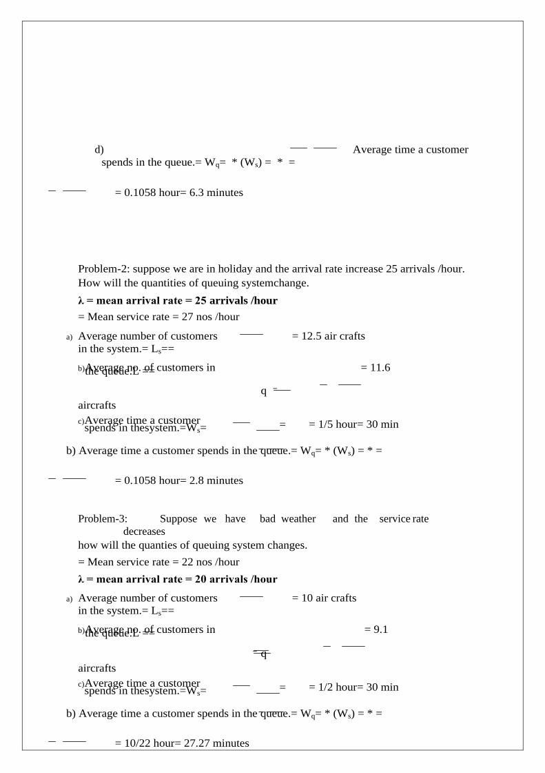
d) Average time a customer
spends in the queue.= Wq= * (Ws) = * =
= 0.1058 hour= 6.3 minutes
Problem-2: suppose we are in holiday and the arrival rate increase 25 arrivals /hour.
How will the quantities of queuing systemchange.
λ = mean arrival rate = 25 arrivals /hour
= Mean service rate = 27 nos /hour
a) Average number of customers
in the system.= Ls== = 12.5 air crafts
b) Average no. of customers in the queue.L ==
= 11.6
q
aircrafts
c) Average time a customer spends in thesystem.=Ws=
= = 1/5 hour= 30 min
b) Average time a customer spends in the queue.= Wq= * (Ws) = * =
= 0.1058 hour= 2.8 minutes
Problem-3: Suppose we have bad weather and the service rate
decreases
how will the quanties of queuing system changes.
= Mean service rate = 22 nos /hour
λ = mean arrival rate = 20 arrivals /hour
a) Average number of customers
in the system.= Ls== = 10 air crafts
b) Average no. of customers in the queue.L ==
= 9.1
q
aircrafts
c) Average time a customer spends in thesystem.=Ws=
= = 1/2 hour= 30 min
b) Average time a customer spends in the queue.= Wq= * (Ws) = * =
= 10/22 hour= 27.27 minutes

e) Problem-4: A self-service store employees one cahier at its counter. None customers
arrive at an average every 5 minutes while the cashier can serve 10 customers in 5
minutes. Assuming Poisson distribution for arrival rate and exponential distribution
for service rate. Find.
159

q
a) Average number of customers in thesystem.
b) Average no. of customers in thequeue.
c) Average time a customer spends in thesystem.
d) Average time a customer spends in thequeue.
Arrival rate = λ = 9/5 customers per minute= 1.8 customers/minute service rate =
= 10/5 customers per minute= 2.0 customers/minute
a) Average number of customers in the system.= Ls= = = 9customers
b) Avg.no. of customers in
the queue.L = =
= 8.1
customers
c) Average time a customer spends in thesystem.=Ws=
= = 5 minutes
b) Average time a customer spends in the queue.= Wq= * (Ws) = * =
= 4.5 minutes
Problem-5: At a certain petrol pump, customers arrive according to a poisson process
with an average time of 5 minutes between arrivals. The service time is exponentially
distributed with mean time of 2 minutes.on the basis of this information. Findout
a) What would be the average que length?Lq
b) what would be the average no of customers in the queueing systemLs
c) What is the average time spent by a car in the petrol pump?Ws
d) What is the average waiting time of a car before receiving petrolWq
e) Solution: ths is an M/M/! queueing model .
Average inter arrival time = 5 minutes
λ = mean arrival rate = 1/5 units/minutes =( 1/5 )*60 = 12 units/hour average
service time = 2 minutes
Mean service rate =
Since λ <
, the steady state solution exists.
L
q
=
Average
queue
length ==
= 4/5 customers
Ls = average no of customers in the queue system= = =
= 2/3 customers
Average time spent in the
petrol pump = Ws = = =
= 1/18 hour= 3.33 minutes

c) Average waiting time of a c* = ar before receiving petrol = Wq= * (Ws)= *
=
1/45 hour = 1.33 minutes
160

Problem: 6 at a certain petrol pump , customers arrive according to a Poisson process
with an average time of 55 minutes between arrivals. The service time is
exponentially distribution with mean time of 2 minutes.Find
a) The average queue length (Lq)
b) The average no. of customers in the queueing system (Ls)
c) Average time spent a customer in a pertrol pump. (Ws)
d) Average time of a customer before receiving the service(Wq)
e) If the waiting time in queue is 4 min, a second pump will be considered. What should
be the arrival rate for scondpump.
Solution: this is an (M/M/1) : ( λμ
AVERAGE INTER ARRIVAL TIME == 5 MIN λ = 1/5 nos per minute
= 12 nos / hour
μ = mean service rate = ½ nos per minutes
= ½ * 60 = 30 nos per hour As λ < μ , the steady state
solution exists.
λ2
122 4 a)AveragelengthofQueue=
Lq(λ)
30(30 1
2)
nos 15
b) Average length of system L λ
12
2nos s (λ) (3012) 3
c) Average time spent in the petrol pump (system)= Ws=
W 1 1
1
hour 3.33min s (λ) (30 12)18
d) Average waiting time of customer in queue ie before receiving the service =Wq=
W λ
1
1
hour 1.33min q (λ) 30(3012) 45
Or
W
q
W
1 3.33 2 1.33min
s
e) To open second pump Wq
λ1 4
W
1q 4mλ1 hour 15 ( )
1 λ1

15hour
30(30λ1)
λ160/320nos/hour or int erarrivaltime 3min
161

M!
n0
Model-II: Single channel Finite population model with Poisson arrivals and
Exponential service times ( M:M:1) : ( N / FCFS)
In some cases , units arrive from a limited pool of potential customers. Once a unit
joins the queue, there is one less unit which could arrive , and therefore the probability
of an arrival is lowered. When a unit is served, it rejoins the pool of potential
customers, and the probability of an arrival is there by increased. As a rule of thumb,
if the population is less than 40, the equations for finite population should be used.
Although the concepts are same as those for infinite populations, some of the terms
are different and the equations required for analysis are different.
One distinct difference is that the probability of an arrival depends upon the number
of potential customers available to enter the system.
Let the total potential customers population is M,
The no. of customers already in the queuing system = n
Then any arrival must come from M-n number , that is not yet in the system. 1
1. The probability of an empty system = P0=nM
M ! (l)
n0 (M n)! u
M ! ( λ
) 2. The probability of n customers in the system Pn=
(M n)! λ nP0(Mn)!( )
nM M! λ
(M n)!
(
)
nM 3) Ls= Expected numberofcustomers in thesystem. nPnn0
λ 4) Expected Number of customers in the queue= Lq= Ls- =
M
(1P ) λ
λ
Lq= Ls-
λ 0
Lq=
M λ
(1P )
W
s
=
λ 0
Ls= λ
W =
W - 1
=
n
n
n

Ls - 1= (Lqλ)*11Lq
q s λ λ λ λ
Problem-5: Amechanic repairs four machines. The mean time between service
requirements is 5 hours for each machine and forms an exponential m distribution. The
mean repair time is 1 hour and also follows the same distribution pattern. Machine
downtime costs Rs 25 per hour and
162

0.2) 0.2) 0.2) 0.2)
2 3 4
mechanic costs Rs55 per day.
i. Find the expected no. of operatingmachines
ii. Determine the expected down time cost perday.
iii. Would it be economical to engage two mechanics, each repairing only two machines.
Solution: This situation involves finite population
When mechanic serving 4 machines M = 4 Arrival rate = λ = 1/5 = 0.2
Service rate
Let us find the probability of an empty system
P0=
1 nMM!
=
n4 n
1 4! 0.2n
(M ( ) ( )
n
0
=
n)! u
n0 (4 n)! 1
1
14!( 1 4! (
2 4! (
3 4! (
4 3! (42)! (43)! (4 4)!
= 1
1 4* 0.2 4*3(0.2) 4*3* 2*(0.2) (4*3* 2*1)(0.2)
0.40
a) Expected number of broke down machines in the system Ls=
L
s
=
4
1 (1 0.4) 4 5* 0.6 1
0.2
the expected number of operating machines in the system = 4-1 =3
b) Expected down time cost per day ( assuming an 8 hours perday)
= 8 * Expected number of broken down m/cs * Rs 25 per hour= 8*1*25 = Rs 200 per
day
c) When there are two mechanics each serving two machines ieM=2
l

P0=
1 nMM!
=
n2 n
1 2! 0.2n
(M ( ) ( )
n
0
n)! u
1
n0 (2 n)! 1
1
2!2!(0.2)12!(0.2)
2 2!2!(0.2)12!(0.2)
2
= 2! (1)! 2!(1)!
1 1 0.68 1 2 * 0.2 2 * 0.04 1.48
It is assumed that each mechanic with his two machines constitute a separate system with
no interplay.
163
l

0.2
λ
M
(1P )
a) Expected number of
machines in the system
Ls=
λ
λ
1 c.
0
= 2 1
(10.68 ) 0.4
Therefore the expected down time / day = 8 * 0.4* no of mechanics = 8*0.4*2 = 6.4
hr/day The total cost with two mechanics = Rs 2 * 55 + Rs 6.4 *25 = 110+160= 270 per
day
Total cost with one mechanic = Rs 55 +Rs 200 = Rs 255 per day ( minimum)
Hence use one mechanic is economical Uses of two mechanics are not economical.
MODEL-3: M/M/C System : (
Let Arrival rate = λ customers per unit time service rate = = customers per unit
minute
both population size , queue size can be
no. of servers = C ( C >1)
The steady state probabilities exists if
2 2 W q (λ)
W
q
5
1
0
(
1
0
5
)
λ2
1
week 10 12
2 4
Lq
(λ)
30(30
12)15
Lλ 12 2
s (λ) (3012) 3
W 1
1
1
hour 3.33min s (λ) (30 12)18
W λ
1
1
hour 1.33min

)
q (λ) 30(3012) 45
W
q
W
1 3.33 2 1.33min
s
λ1
4 1 λ1
4 1 1
W
1q4mλ
1
hour hour15 15
hour 1.33min λ
1 1530(3012) 45
1 λ1
15hour
30(30λ1)
λ160/320nos/hour or int erarrivaltime 3min
(λ < c )
164
( ) (

λ
λ
P01
λ n
λc
c 1 (
) (
)
* 1
n 0 n! c! (1)
λ n
λ( )
λ
λ Lq 2P0
(c1)!*(c λ)
5 2c
5*10*( ) 3 1
Lq
10 2 *
(2 1)!*(2*105) 530
Theprobabiliti
es aregiven
byLqP0
1
λ c
(
)
c
!
*
(1)2
n ( )
P
0nc
P =n! o
n n
( ) c!c
ncP0
n c
λ n
( ) The expected number of customers in queue L
q P0
c!*
(1)2
λ(λ/)c
λ 1. Theexpectedno.ofunitsinthesystem=L
s(c1)!*(cλ)
2*P0
----- eqn-1
2. The expected queue length L = L mean number being served = Ls - λ
= Ls -λ
q s-

165

1
q 2 0
λ n
λ( ) =
λ
λ
---- eqn-2 Lq 2 P0
(c1)!*(c λ)
Lq
λ c
λ(
)
2P0
(c 1)!*(cλ)
Pn
λ n
(
)
2P0
n!(c 1)!*(cλ)
λ 1
P
n
(
)
P0
λ 5 1
3 3
P(
)P0( ) *10 5100
λ c
() 1
3) Expectedwaitingtimeinthequeue=Wq
=Lq*λ=
(c1)!*(cλ)2 P0
---- eqn-3
λ c
(
) 4) Expected waiting time in the system Ws = W + = +
P (c1)!*(c λ)
Theexpectedwaiti
ngtimeinthequeue
=Wq=

λ * Lq
1 the exp[ected waiting time in the system = Ws = Wq +
the expected no. of customers in the system = Ls = λ Ws
166

λ ( Wq + 1
)= λ ( + 1
)= = λ
λ
= Lq +
Problem: (M/M/C): ( A petroleum company is considering expansion of its one
unloading facility at its refiner. Due to random variations in weather, loading delays, ships
arrivingattherefinerytounloadcrudeoilarriveatarateof5shipsperweek.Theservicerateis
10 ships per week. Assume arrivals follows a poisson process and the service time is
exponential.
a) Find the average time a ship must wait before beginning to deliver its cargo to the
refinery.(Wq)
b) If second birth is rented , what will be the average no. of ships waiting before being
unloaded.
c) What would be the average time a ship would wait before being unloaded with twobirths.
d) What is the average no. of idle births at any specified time. Solution:
Mean arrival rate λ = 5 ships/ week Mean service rate = = 10 ships per week
a) The expected waiting time (Wq) before
ship begins to unload crude oil isWq=
λ
(λ)
=
W
q
5
1
0
(
1
0
5
)
1
week 10
b) With a second berth , the queueing model is an M/M/2system
λ
C
5
2
*
1
0
1/4
1
P0 λ
n λ
c
c
1
(
)

( ) *
1
n
0
=
P
0
n!
(5/10)0
c!
(1 )
(5/10)1
1 (5/10)12
3 (5/10)
2 10*2 5
( ) 0! 1! 2! 2! 10*25
λ n
Lq =
λ( )
λ
λ
Lq 2 P0 (c1)!*(c λ)
167

5 2c
5*10*( ) 3 1
=Lq
10 2 *
(21)!*(2*105) 530
c) W
q=
Lq1*
1
1week
λ 30 5150
d) If there is no ship in the system then boh the births areidle.
If there is only one ship in the system , one of the births is empty.
P
n
λ n ( )
n
!P
0
λ1
0 < n < C
(
) 51
33 P1=
Pn
P0=(
)*
10 510
Hence the expected number of idle berths is = 2 * P0 + 1 * P1
= 2 * (3/5) + 1* (3/10) = 15/10 = 1.5
Problem-2: A super market has two girls ringing up sales at the counters. If the service
time for each customers is exponential with mean 4 minutes, and if people arrive in a
Poisson fashion at the rate of10/hour
a) What is the probability of having to wait forservice.
b) What is the expected percentage of idle time for eachgirl?
c) Find the average length and the average number of units in thesystem.
****

168

SIMULATION
Simulation is the representative model for real situations. Definition: Simulationisarepresentationofrealitythroughtheuseofamodelorotherdevicewhichwill
react in the same manner as reality under a given set of conditions.
Simulation is the use of system model that has designed the characteristics of reality in
order to produce the essence of actualoperation
Example: the testing of an air craft model in a wind tunnel from which the performance of
the real aircraft is determined for being under fit under real operating conditions. In the
laboratories, we often perform a number of experiments on simulated models to predict the
behavior of the real system under true environments.
According to Donald G. Malcolm, a simulated model may be defined as one which depicts
the working of a large scale system of men, machines, materials and information operating
over period of time in a simulated environment of the actual real world conditions.
TYPES OF SIMULATION
Analogsimulation Computer simulation ( System Simulation) i. Deterministicmodels
ii. Stochastic model
iii. Static models
iv. Dynamic models
NEED FOR SIMULATION
Simulation techniques allow experimentation with a model of real-life system rather than
the actual operatingsystem.
Sometimes there is no sufficient time to allow the actual system to operateextensively.
The non-technical manager can comprehend simulation more easily than a complex
mathematical model.
T
he use of simulation enables a manager to provide insights into certain managerial
problems.
SIMULATION PROCESS
Step-1: First define and identify the problem clearly.
Step-2.Secondly, list the decision variable and decide on rules of the problem. Step-3.
Formulate the suitable model for the given problem.
Step-4. Test the model and compare its behavior with the behavior of real problem
situation. Step-5. Collect and identify the data required to test the model.
Step-6. Execute (run) the simulation model.
Step-7’ the results of simulation run are then analyzed. If the simulation run is complete,
then choose the best course of action, otherwise , required changes are done in model
decision variables, design or parameters and go to step-4.
Step-8. Run the simulation again to find the new solution. Step-9. Validate the simulation.
169

LIMITATION OF SIMULATION
Optimum results cannot
The another difficulty lies in the quantification of thevariables.
In very large and complex problems, it becomes difficult
to make the computer program on account of large
number of variables and the involved inter-relationships
amongthem.
Simulation is comparatively costlier, time consuming method in manysituations.
TYPES OF SIMULATION MODELS
Deterministic models: In this type of models, the input and output variables cannot be random variables and can
be described by exact functional relationships.
Probabilistic models
In these models, method of random sampling is used. This technique is called ‘Monte-
Carlo Technique.
S tatic Models:
In these types of models, the variable time cannot be taken into account consideration.
Dynamic Models:These models deal with time varying interaction.
PHASES OF SIMULATION MODEL
Phase-1: Data collection
Data generation involves the sample observation of variables and can be carried with the
help of following methods.
Using random numbertables.
Resorting to mechanical devices. )example: rouletteswheel)
Using electroniccomputers
Phase -2. Book-keeping Book-keeping phase of a simulation model deals with updating the system when new
events occur, monitoring and recording the system states as and when they change, and
keeping track of quantities of our interest (such as idle time and waiting time) to compute
the measure of effectiveness.
GENERATION OF RANDOM NUMBERS
For clear understanding, the following parameters are be defined
Random variable: it refers to a particular outcome of anexperiment.
Number::it refers to a uniform random variable or numerical value assigned to a random
variable following uniform probability density function. ( ie., normal, Poisson,

exponential,etc).
Pseudo-random Numbers: Random numbers are called pseudo-random numbers when they
are generated by some deterministic process but they qualify the pre-determined statistical
test for randomness.
170

MONTE-CARLO SIMULATION- STEPS INVOLVED
i. First define the problemby
Identifying the objectives of the problem
Identifying the main factors having the greatest effect on the objective of the problem
ii. Construct an appropriate modelby
Specifying the variables and parameters of the model Formulating the suitable decision
rules.
Identifying the distribution that will be used. Specifying the number in which time will
change,
Defining the relationship between the variables and parameters.
iii. Prepare the model forexperimentation
Defining the starting conditions for the simulation Specifying the number of runs of
simulation.
iv. Using step1 to step 3, test the modelby
Defining a coding system that will correlate the factors defined in step1 with random
numbers to be generated for simulation.
Selecting a random generator and creating the random numbers to be used in the
simulation. Associating the generated random numbers with the factors as identified in
step1 and coded in step4.
v. Summarize and examine the results as obtainedin.
vi. Evaluate the results of thesimulation
vii. Formulate proposals for advice to management on the course of action to be adopted and
modify the model, ifrequired.
APPLICATION OF SIMULATION
Simulation model can be applied for Solving Inventoryproblems
Simulation model can be applied for solving Queuingproblems
Simulation model can be applied for solving Inventory problems:
Problem-1: A bakery keeps stock of populr brand f cake. The previous experience shows
the daily demand pattern for the item with associated probabilities , is as given below:
Daily demand 0 1
0
2
0
3
0
4
0
5
0
Probability 0
.
0
1
0
.
2
0
0
.
1
5
0
.
5
0
0
.
1
2
0
.
0
2
Use following sequence of random numbers to simulate the demand for next 10 days. Random

numbers: 25, 39, 65, 76, 12, 05, 73, 89, 19, 49 .
Estimate the daily average demand for the cakes on the basis of the simulated data.
Solution: Using the daily demand distribution, we first obtain a probability distribution as
shown in
171

table-1.
Daily
demand
Proba
bility
Cumul
ative probability
Randon
number Interval
0 0.01 0.01 00
10 0.20 0.21 01 - 20
20 0.15 0.36 21 - 35
30 0.50 0.86 36 - 85
40 0.12 0.98 86 - 97
50 0.02 1.00 98 - 99
Next to conduct the simulation experiment for demand take a
sample of 10 random numbers from a given random numbers,
which represent the sequence of 10 samples. Each random sample
number represents a sample of demand . The simulation
calculations for a period of 10 days are given intable-2.
Days Random
number
Simulated
demand
1 40 30 Since R,no 40 falls in
the interval of 36-85
2 19 10
3 87 40
4 83 30
5 73 30
6 84 30
7 29 20
8 09 10
9 02 10
10 20 10
Expected demand = total /10 =220/10= 22 units per day
Problem-2: A company manufacture around 200 mopeds ,
depending upon the availability of raw material and other
conditions. , the daily production has been varying from 196
mopes to 204 mopeds, the probability distribution is as
givenbelow,
Production
per day . 196
197
198
199 200 201 202 203 204
Probability 0.05
0.09
0.12
0.14 0.20 0.15
0.11
0.08
0.06
The finished mopeds are transported in a specially designed
three-storied lorry that can accommodate 200 mopeds. Using
the following 15 random numbers 82, 89, 78, 24, 53, 61, 18,
45, 23, 50,77, 27, 54. Simulate the mopeds waiting in the

factory. what will be the average number of mopeds waiting in
the factory ?. What will be the number of empty spaces waiting
in the factory?. What will be the number of empty spaces in
thelorry?.
172

Solution:
a) Using production per day distribution, the daily production is shown in table.
Production
/ day Probabili
ty. Cumilative probability
Random number interval
196 0.05 0.05 00 – 04
197 0.09 0.14 05- 13
198 0.12 0.26 14-25
199 0.14 0.40 26-39
200. 0.20 060 40-59
201 0.15 0.75 60 -74
202 0.11 0.86 75-85
203 0.08 0.94 86-93
204 0.06 1.00 94-99
Based on the given 15 random numbers’, simulation experiments of production per day is shown in table
days
Random number
Production
per day
No. of moped waiting
Empty space in the lorry
1 82 202 2 -
2 89 203 3 -
3 78 202 2 -
4 24 198 - 2
5 53 200 0 0
6 61 201 1 -
7 18 198. - 2
8 45 200 00 -
9 04 196 - 4
10 23 198 - 2
11 50 200 0 -
12 77 202 2 -
13 8 199 1- 1
14 54 200 0 1
15 10 197 - 3
total 10 14
173

Average number of mopeds waiting in the factory = 1/15(
2+3+2+1+2)= 10/15 = 0.66 = 1 mopeds approx
Average number of empty spaces in the lorry = 14/15 =0.86
Problem-3: A book store wishes to carry a particular book in
stock. The demand of the book is uncertain and there is a lead
time of 2 days for stock replenishment. The probabilities of
demand are given below: Demand (units/day)
0 1 2 3 4
Probability 0.05 0.10 0.30 0.45 0.10
Each time an order is placed, the store incurs an ordering cost of
Rs 10 per order. The store also incurs a carrying cost of Rs 0.50
per book per day. The inventory carrying cost is calculated on the
basis of stock at the end of each day. The manager of the book
store wishes to compare two options for his investmentdecision.
a) order 5 books when the present inventory plus any outstanding order falls below 6books.
b) order 8 books when the present inventory plus any outstanding order falls below 6books.
Currently (beginning of the 1st day) the store has a stock of 8
books plus 6 books ordered two days of and are expected to
arrive the nextday.
Carry out simulation run for 10 days to recommend an
appropriate option. You may uses random numbers in the
sequences, using the first number for day one 89, 34, 78, 63,
61, 81, 39,16, 13,73.
Solution: using the daily demand distribution , we obtain probability distribution as shown in table-1.
Daily demand
Probability
Cumilative probability
Random number interval
0 0.05 0.05 00 – 04
1 0.10 0.15 0 5- 14
2 0.30 0.45 15 - 44
3 0.45 0.90 45 - 89
4 0.10 1.00 90- 99
Case-A: The stock in hand is of 8 books and stock on order is 5 books (Expected next day)
Random number
Daily demand
Opening stock
Receipt Closing stock in hand
Order quantity
Closing stock
89 3 8 - 8-3
=5 5 5
34 2 5 5 5+5-
2=8 - 8
78 3 8 - 8-3=5 5 5

63 3 5 5 5+5-3=7
- 7
61 3 7 - 7+0-3=4
5 4
81 3 4 5 4+5-3=6
- 6
39 2 6 - 6-2=4 5 4
174

16 2 4 5 4+5-2=7
- 7
13 1 7 - 7-2=6 - 6
73 3 6 - 6-3=3 - 3 TOT;=55
Since 5 books have been ordered four times as shown in table . therefore the totak ordering
cost is
= 4* Rs10= Rs 40/-
Closing stock of 10 days = 55 books. Therefore ., the holding cost at the rate of Rs 0.5 per
book per day is = 55* 0.50 =Rs27.5
Total cost = Rs 40 + 27.50 = 67.50
Case-B: Order 8 books when the present inventory plus any outstanding order falls
below 6 books.
The stock in hand is of 8 books and stock on order is 5 books ( Expected next day)
Random number
Daily demand
Opening stock
Receipt
Closing stock in hand
Order quantity
Closing stock
89 3 8 - 8-3 =5 8 5
34 2 5 8 5+8-2=11
- 11
78 3 11 - 11-3=8 - 8
63 3 8 - 8-3=5 8 5
61 3 5 8 13-3=10
- 10
81 3 10 - 10-3=7 - 7
39 2 7 - 7-2=5 8 5
16 2 5 8 13-2=11
- 11
13 1 11 - 11-1=10
- 10
73 3 10 - 10-3=7 - 7 TOT;=79
Eight books have been ordered three times, as shown in table, when the inventory of books at the
beginning of the day plus outstanding order is less than eight.
Therefore total ordering cost is =no. of orders * ordering cost per order = 3 * 10 = Rs 30.00 The
closing stock of 10 days is = 71 books
Therefore , the holding cost @ rs0.50 per book per day is = Rs 71*0.50 = 35.50
The total cost for 10 days = Rs 30.00 + 35.50 = Rs 65.50 this option -case-B is lower than case-A.
Select option case-B

175

Simulation model can be applied for solving Queuing problems
• Event list: to help determine what happensnext:
– Tracks the future times at which deferent types of eventsoccur.
– Events usually occur at randomtimes.
• The randomness needed to imitate real life is made
possible through the use of random (pseudo-
random) numbers (more on thislater).
STEPS INVOLVED IN SIMULATION
• The simulations are carried out by the followingsteps:
– Determine the inputcharacteristics.
– Construct a simulation table.
– For each repetition I, generate a value
for each input, evaluate the function,
and calculate the value of the
responseYI.
• Simulation examples will be given in
queuing, inventory, reliability and net
workanalysis. •
APPLICCATION OF SIMULATION FOR QUEUING MODELS
Simulation of Queuing Systems
• A queuing system is described by its
calling population, nature of arrivals,
service mechanism, system capacity
and the queuingdiscipline.
• In a single-channelqueue:
– The calling population isinfinite.
– Arrivals for service occur one at a
time in a random fashion. Once they
join the waiting line they are
eventuallyserved.
• Arrivals and services are defined by
the distribution of the time between
arrivals and servicetimes.
Simulation of Queuing Systems
• Assume the only possible service times
are 1, 2, 3 and 4 time units and theyareequally likely to occur, with

input generatedata:das:
176
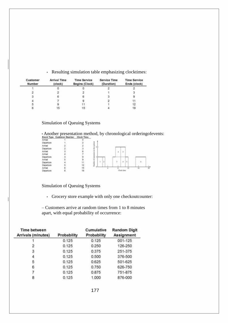
• Resulting simulation table emphasizing clocktimes:
Simulation of Queuing Systems
• Another presentation method, by chronological orderingofevents:
Simulation of Queuing Systems
• Grocery store example with only one checkoutcounter:
– Customers arrive at random times from 1 to 8 minutes
apart, with equal probability of occurrence:
177