instantaneous pressure distribution around a · pdf fileinstantaneous pressure distribution...
TRANSCRIPT

INSTANTANEOUS PRESSURE DISTRIBUTION AROUNDA SPHERE IN UNSTEADY FLOW
C1
Leslie S. G. Kovasznay, Itiro Tani, Masahiko Kawamura andHajime Fujita
Department of MechanicsThe Johns Hopkins University
December 1971
.,DDCOffice of Naval Research .11 j)Washington D. C. 20360 D *Ljq 119
B
Technical Report: ONR No. N00014-67-0163-002. Distribu'tion of thizdocument is unlimited. The findings of this report are not to be conftruedas an official Department of Navy position unless so designated by tl-eirauthorized documents.
"ApP"xi.' for public MO ..
FDistribution Unlinuted

pt
II
INSTANTANEOUS PRESSURE DISTRIBUTION AROUND
A SPHERE IN UNSTEADY FLOW
Ii
Leslie S. G. Kovasznay. Itiro Tani, Masahiko Kawamura andHajime Fujita
Department of MechanicsThe Johns Hopkins University
December 1971
Technical Report: ONR No. N00014-67-0163-00Z. Distribution of this
document is unlimited.
'I

ABSTRACT
\In oirder to stu-dy efrfects of velocity and acceleration of a flow
to the pressure on an obstacle, a small sphere with a pressure hole
was placed in a periodically pulsating jet. Both the instantaneous
pressure on the sphere and the inst.antaneous velocity of the flow:1 field when the sphere was absent were measured. By using periodic
sampling and averaging techn.iques, only periodic or deterministic
component of the signal was recovered and any random componentI
caused by turbulence suppr-essed. The measured surface pressure
was expressed in terms of this measured velocity and acceleration •
of the flow. A simple inviscid theory was developed and the experimental
results were compared with it.
IN
I!

12 a' ,-';
ACKNOW LEDG EMENTS
This research was supported by frI. S. Office of Naval Research
under contract No. N00014-67--0163-0002.
The autEhors would like to express thanks to Mr. L. T. Miller
for help in technical aspect, and to Mrs. C. L. Grate for the typing
of the text.
> J

TABLE OF CONTENTS
R PageABSTRACT
ACKNOWLEDGEMENTS
LIST OF ILLUST RATIONS
I. INTRODUCTION 1
2. EXPERIMENTAL FACILITY AND PROCEDURE z
3. EXPERIMENTAL RESULTS 5
4. THEORY 7
5. DISCUSSION 11
6. CONCLUSIONS 13
LIST OF REFERENCES
ILLUSTRATIONS
I:J
~ 41

LIST OF ILLUSTRATIONS
Fig. 1 Pulsating flow generator
Fig. 2 Pulsating velocity of the jet at x = 6 cm, pulsatingfrequency 450 Hz
Fig. 3 Schematic diagram of data acquisition
Fig. 4 Three sphere models and condenser microphone
Fig. 5 Rotatior of the model
Fig. 6 Calculated frequency response of microphone with cavities
Fig. 7 Mean velocity distribution of steady jet at x = 3 and 6 cm
Fig. 8 Instantaneous velocity distribution of pulsating jet atx = 5 cm, f = 450 Hz
Fig. 9 Pulsating velocity amplitude and phase velocity along thecenterline of jet at f = 450 Hz
Fig. 10 Pressure distribution around the sphere in steady flow(so.id line indicates inviscid theory)
Fig. II Coefficients A and B at x = 3 cm, f = 450 Hz
Fig. 12 Coeffici.ents A and B at x = 3 cm, f = 300 Hz
Fig. 13 Coefficients A and B at x 6 cm, f = 350 Hz
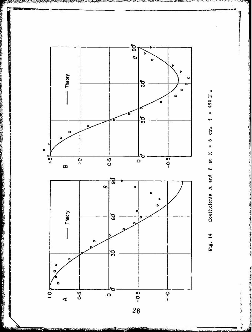
Fig. 14 Coefficients A and B at x = 6 cm, f = 450 Hz
Fig. 15 Streamlines theoretical model for = ka =
N
"4'
,/
NM

1. INTRODUCTION
Measurement of the instantaneous value of the static pressure
inside a turbulent flow is still an unresolved problem because the
pressure probe placed in the unsteady flow field represents a solid
boundary and the surface pressure at a point always contains important
contributions from the inertial effects in the flow around the body. For
steady flows it is relatively easy to design "static" probes that read
the static pressure by using potential theory to calculate the pressure
distribution around the body of the probe, but the sa;n-e locations do
not give instantaneous static pressure in unsteady flow.
In order to understand better the behavior of small probes placed
in unsteady flows, an experimert was performed in a relatively simple
configuration. A small sphere was placed in a pulsating jet and the
instantaneous surface pressure fluctuations were measured. Since
in such a flow there is a strong random component of fluctuations due
to the turbulence, a special signal processing technique, namely periodic
sampling and averaging was performed on all signals in order to enhance
the periodic (or deterministic) componerit and to suppress the random
component.
Furthermore, in order to provide a guide for the assessment of
the results a simple inviscid theory was developed and the experirrental
results were compared with it.
\'
• • •i • • Y• .. . •---~'-•, -i''• ' 'i' ' • ... .. , -.......... ..

2 71Ai
Z. EXPERIMENTAL FACILITY AND PROCEDURE
T'he time-dependent flow for measurements, the pulsating flow,
is produced by the scheme indicated in Fig. 1. The stez.dy air flow
provided by the centrifugal blower is divided into two streams, the
one flowing through the duct D1 and the other through the duct D7.
One flow component is discharged through the duct D1 and is periodically
ixtercepted by a rotating disc with 16 holes. As a result periodic
pressure fluctuations are induced also in the other branch, D 2 , through
which the other flow component is discharged and pulsating air jet is
S~produced. The frequency and •.mplitude of the velocity fluctuation in
I the jet can be varied within limits varying the speed of the rotating
disc and the stand-off between the disc and the nozzle attached to Dl.
The pulsating velocity of the jet was measured by a constant
(1) (2)temperature hot-wire anemometer followed by a linearizer.
Since hot-wire signal as obtained from the output of the linearizer
still contains random fluctuations due to turbulence in the jet, special
signal processing technique, periodic sampling and averaging, was
performed by using "Wavefrom Eductor" Model TDH9 of Princeton
Applied Research. The output of that instrument gives the ensemble
ave'" c.e of a large number (typically 1000 - 2000) of sweeps and the
random compor-nt is correspondingly reduced by a factor of
4F2000 or 30-40. As the result most of the random components is

•s 3.
suppressed and only periodic or deterministic component is recovered.
The necessary synchronizing pulses were obtained from the rotating
disc by using a photo-cell pick up. Fig. 2 shows an example of the
periodic velocity fluctuation measured at a distance x = 6 cm from
the nozzle at a pulsating frequency of f = 450 Hz. The same technique
was used to obtain the periodic pressure fluctuation on the sphere as
described below. Schematic diagram of the instruntentation is shown in
Fig. 3.
Three spheres of the same diameter but with a pressure hole at
different locations along the meridian were used as models. They are
designated as S, 0 and R as shown in Fig. 4. The diameter of the
sphere is 6.35 mm and the diameter of the pressure hole is 0.5 mm,
located at the meridian angle e = 0° (opposite stem), 450 and 900 foi-
S, 0, and R respectively. The pressure hole is connected to a frequency
modulated condenser micnphone through the stem as shown in Fig. 4,
and the pressure fluictuations is converted to the electrical signal. In
earlier period of the experiment a transistiorized version of the circuit
used by Einstein and Li (l) was used as the FM oscillator and the detector.
In later period an improved circuit with the carrier frequency within the
range of commercial FM broadcast was built into the probe as shown in
Fig. 4 and an FM receiver EICO CORTINA 3ZOO was used as the detector.
The sphere was rotated around its center by a lathe turn table up
to a maximum angle of + Z0o (Fig. 5) so by using all three models it
SI-4

4.
was possible to orient the pressure holes on the sphere at every 5-
between-20 0 to 1100. The overall static sensitivity was found to be
57 and 2.4&S.V/Jgtr respectively. The overall frequency characteristic..
of the pressure probe depends on the diameter and length of the pipe
leading to the microphone as well as on the volume of the cavity in
front of the microphone diaphragm. Fig. 6 shows the calculated
frequency characteristics for the combination of a pipe of diameter
1. 0 mm and length 20. 5 mm and for two values of the cavity of volume
1. 65 and 89. 1 mm 3 , respectively. Resonances occur around 800 Hz
and 2500 Hz respectively. The dynamic sensitivity of the probe would
have been best obtained by the Coupler Method, which is based on a
comparison with a standard microphone. Unfortunately, however, no
standard microphone was available, so an alternative procedure was used
by utilizing a theoretical relation obtained for a sphere. According to the
theoretical calculation given in a later section, the pressure fluctuation
on a sphere is made up of two terms, one being proportional to the
fluctuating velocity itself and the other one proportional to the time derivative
of the :luctuating velocity. At the forward stagnation point the non-
dimensional coefficients of the two terms calculated by the theory are 1. 0
and 1. 5 respectively. By assuming a phase lag in the nmeasured pressure
fluctuation due to the lead pipe and the cavity volume, the ratio of the two
coefficients, dynamic sensitivity~for the stagnation point was calculated
as described in the following chapter from the fluctuating velocity and its
time derivative obtained by a hot-wire placed at the location of the sphere
center but in the aý.scnce of the sphere. T.'.- phase lag so determrined
- - - -

5.
varied between 10 and 300, and the dynamics sensitivity was found to be
10% - 40% higher than the static sensitivity.
3. EXPERIMENTAL RESULTS
First measurements were made within the jet which is discharged
from the duct DZ through a contracting nozzle to the ambient air (Fig. 1 ),
for a mean velocity of about 20 m/s at the jet axis. Fig. 7 shows the
velocity distribution across the steady non pulsating jet at two stations,
x = 3 and 6 cm do.rr.-"-earn from the nozzle. The core of the jet,
defined as the region in which the velocity is greater than 90% of the
velocity on the axis (To has a diameier 1.55 cm at x = 3 crn and 1.28 cm
at 6 cm, respectively. Fig. 8 shows the instantaneous velocity profiles
across the fluctuating jet at a station x = 5 cm for a frequency of 450 Hz.
The core diameter defined as above is about 1. 20 cm, which is a little
less than that of the steady jet. Fig. 9 shows the stream'vise variation
ef the amplitude and phase velocity of the velocity fluctuation along the
jet axis. Circles are described to indicate the location and size of the
sphere. When the sphere is placed at x = 3 cm, the ratio of the core
diameter of the steady jet to the sphere diameter is 2. 4, but the amplitude
of velocity fluctuation still varies by about 30 per cent over the region
occupied by the sphere. When the sphere is placed at x = 6 Lm, the
ratio of the diameters is reduced to 2. 0, but the variation of th.. amplitude
cf the velocity fluctuation becomes negligible. The phase velocity determined
by two-hot wires separated by a fixed streamwise distance is approximately

6.
constant over the region covered by experi;-nent. The actual value was
13. 2 m/s, about two thirds of the mean velocity at the jet axis. The
phase velocity is regarded as the velocity of the travelling vortex ring
produced at the nozzle traveling downstream.
Fig. 10 shows the mean (D. C.) pre sure distribution on the sphere
placed at x = 3 cm in the steady jet. The calculated value are also shown.
The Reynolds number based on the sphere diameter and the velocity on the
axis is ý---8 .8 x 103. As shown later in the theory, the instantaneous
surface pressure at a point can be expressed as
P=p9 + ALU' -t- B13 f U-2-
where U is the instantaneous strearnwise velocity component a is
the diameter Mf the sphere, A and B are the coefficients of
the contribution from the instanteaneous velocity and from the
instantaneous acceleraticn rm:spectively.
The coefficients A and B are strong functions of the coordinates
(the azimuth angle) and they may also weakly depend on the Rr-nolds
number.
For the periodically pulsating flow, the above equation can be written
more specificaly asP'fz)AU'-) -- A o-CO")
2
where /TT = Period
dat
for a particular location on the sphere. After the periodic sampling and
averaging, values of all oi pZ) , l(-r and were
-S. -T

7.
sampled at ten equaliy spaced points over the entire period, and the
coefficient A and B were determined by the method of least square
so that the mean square error
becomes minimum.
Fig. 11 to14 show the experimental values of A and B, the tv o coefficients
of influence. The values determined on the three models S, 0 and R are
indicated in these figures by the symbols of square, circle and triangle,
respectively. Solid curves give the theoretical prediction based on the
assumption of inviscid irrotational flow described in the following chapter.
4. THEOP.
With a view to gaining an insight into the problem, a theory is
developed to predict the pressure acting on a sphere placed in a time-
dependent flow of an inviscid fluid. A solution of the problem relevant
(4)to the subject was treated by Lamb as follows. The pressure p on a
sphere moving g'th time-dependent velocity V in an infinite mass of
fluid at rest a. infinity is given as
( .1 ..oz 9)Y.. - CCsP9.- ai()
"where po is the pressure at infinity, t the time, y the densiLy of fluid,
a the radius of the sphere, and & the ,neridian angle measured from the
rear stagnaion point. Unfortunately, however, the problem treated there
doer not exactly correspond to the present experiment, since the time-

8.
dependent flow that can be readily produced in the laboratory is a steady
uniform flow with sutwrimposed traveling disturbances with no associated
pressure fluctu*itions in the free strea.-n.
It is not difficult to illustrate the possibility of such a time-dependent
flow. With the Cartesian coordinates (X, Y, Z), for example, the
momentum equations are satisfied by ta,.ng a flow field
V = U V = f(x-J t), V = 0 = constant, (2)x 0 y 0 z
which represent a steady flow of velccity U on which a two-dimensional
traveling disturbance is superimposed. No change in pressure is produced
by the disturbance. Since, however, the disturbance is rotational having
a component of vorticity in z-direction, the vortex filaments are stretched
by the introduction of a three-dimensional body such as a sphere. This
means that the "compensating flow" introduced to satisfy the boundary
conditions on the sphere must be also be rotational. It does not seem to
be impossible to find such a compensating flow, but in view of the limited
range of application of the present theoretical calculation, it is doubtful
whether the solution warrants the extra complication involved.
In order to simplify the calculations it is assumed that the disturbance
is fufficiently small, irrotational and traveling with a velocity equal to that
of the steady uniform flow. Using spherical polar coordinates (r, 9, •
such that
X r cost, Y rcinI cos;, Z -- in 9sin, , (3)
the velocity potential is assimed in the form 4
+ =. z (4)

9.
where
~0u~I + ~Cos (5)
is the velocity potential for the steady flow of velocity TI past a sphere0
of radius a with center at origin. The second term
, U.sin k(rcoS V -Uot) I0 (&rsin 1)
is the velocity potential for the superimposed disturbance traveling with
the phase velocity U and wave number k, and finally
is the velocity pe antial for the compensating flow, F is a non-
dimensional constant, I. is the modified Bessel function of the first kind,
Pn the Legendre polynomial of order n, and Cn the non-dimensional
constants (n = 1, 2, 3, . . .) to be determined by applying the boundary
conditions on the sphere. If • is assumed to be small compared to unity,
the disturbance represented by 1, gives a velocity fluctuation of order
7 0- U. for finite values of Arsin 9 , and, when superimpos on the
steady uniform flow, produces a change in static pressure of crder E
which is second order and is considered negligible. Although the velocity
fluctuation increase indefinitely as !k~ifl1 tends to infinity, this does not
stem to affect seriously the results provided that the consideration is
limited to the regior close to the sphere and an additional assumption is
made that ka is small compared to unity, namely, the radius of the sphere
is small compared to the wavelength of the disturbance. Fig. 15 shows
the instantaneous streamlines (with equi-distant values of the Stokes stream
function if,) for the velocity potential ,for a value E I A i

10.
Under the assumption that ka is small, the normal velocity
produced by the disturbance on the sphere is given by expanding eq. (6)
and keeping the first two terms
4 ,CoS19,coS U~t + ~*0-(,3 C0xA'S-T-/r- = a- ,LU os•
which must be cancelled ve the normal velocity calculated from (,flar),.4
The constants in the expression for a are then determined as
The pressure on the sphere is obtained from the equation
-+ FIOtf 2 (8)
S~P 0 beir~g the pressure at infinity. The pressur?• onI the sphere is thus
given by
where
(-5F ?Pr& t jo1 ' br4CS( 5L 6) (0
If the velocity V and the acceleration dVUdt at the location of the sphere
center (r o) are introduced by
Vka. U. 2rs
dt (11) + U
2. r

the pressure on the sphere is expressed in the form
±Z4L(12)
Eq. (12) indicates "Inat the pressure on the sphere consists of two terms,
the one being proportional to the instantaneous dynamic pressure (1/Z))PV .
and the other proportional to the time derivative of velocity Pa(dV/dt). The
coefficient A of the first term is the same as for the classical solution (1),
but the coefficient B of the second term is considerably different.
On writing
i9•--e V=Uo1- L (13)
where B is the meridian angle rmeasured from the forward stagnation
point, and u is the velocity fluctuation, (12) and (10) are written in the
form
2,(14)
-4 5 f- 9 CO:S '8) c05 (-3 - -O'6
5. DISC USSION
In the theoretical calculation it was assumed that E and ka are
small compared to unity, namely, the amplitude of velocity fluctuation is
small compared to the mean velocity on the jet axis, and the radius of
sphere is small compared to the wavelength of velocity fluctuation. These
conditions were not exactly satisfied in the experiment, wherr the
maximum values of E and ka are 0.40 and 0. 63, respectively. Moreover,
the observed phase velocity of velocity fluctuation was only 213 of the mean
velocity, whereas in the theory the phase velocity is assumed to be equal
* -°•~-

to the mean velocity.
In spite of these circumstances, however, the experinental va',.es
of the coefficients A and B agree fairly well with theoretical results
for the sphere location at x = 6 cm (Figs. 13 and 14). The agreement is
I, nc. as good for the location at x = 3 cm (Figs. 11 to 12), and this may be
due to the undesirable variation of the velocity fluctuation amplitude around
that location.
As seen from Fig. 2. the observed velocity fluctuation is not exactly
simple sinusoidal, but a slight distortion in the wave form is apparent that
results in higher harmonics. The distortion increases as the fundamental
frequency decreases. This seems to account for the fact that the root-
mean-square residual error of representing the observed pressure fluctua-
':1 tion by two terms amounts to 10. Z, 9.7 and 6. ' per cent of the fluctuation
- amplitude for the fundamental frequency f = 300 Hz (x 3 cm), 350 Hz
(x =6 cm) and 450 Hz (x = 3 and 6 cm), respectively.
No measurement on pressure was made on the rear side of the sphere,where the separation of flow is expected to -nodify the pressure distribution.
The effect of separation can be traced in the pressure distribution for
meridian angle greater than e = 700, where the experimental value of
A begins to deviate from the theoretical curve (Figs. 13 and 14). On the
other hand, the .xperimental value of B agrees fairly well with the
theoretical result up to as far as • - 900 (Figs. 13 and 14). It is not
certain whether the agreement is real or fortuitous.
fi~~ -~A
N~-

13 .
6. CONCLUSIONS
Measurements of the instantaneous values of the surface pressure
were carried out on a small sphere in a periodic pulsating flow and the
experimental values agreed moderately well with a concurrently developed
inviscid theory. t is apparent from the above theoretical and experimental
work that simila.r calculations can be performed on bodies other than
spherete. or even on a combination of bodies. By judicious choice of
such bodies points may be found on the surface where the coefficienta
A = B = 0 so the measu-ed pressure has no contribution from the
acceleration. Pressure transducers at such points or appropriately
coupled to pressure holes at such points would indicate static pressure
fluctuations in the flow corresponding to the location of the body but with
the body absent quite sirnilarlrly to -tatic probes used in steady flows.
The principal difference is that two terms must be cancelled instead the
usual one in steady flow.

REFERENCES
1. Kovasznay, L. S. G. , Miller, L. T. and Vasudeva, B. R. (1963)A Simple Hot-Wire Anemometer, Project Squid Ted. Rep. JHII-22-P,Dept. of Aerospace Engr., Univ. of Vir&'" :a.
2. Kovasznay, L. S. G.. and Chevrav, R. (1969) Temperature Compensated 2
Linearizers for Hot-Wire Anemometer, Rev. Sci. Inst., Vol. 40, p. 91.
3. Einstein, H. A. and Li, H. (1956) The Viscous Sublayer along a SmoothBoundary, Proc. Arr. Soc. Civ. Engr. Paper 945.
4. Lamb. H. (1945) Hydrodynamics 6th ed., p. 124, Dover.
.I ..
I~' I

BLOWER
----- 1-•
TRIGGERING STATIC HOLEPHOTO CELL I---L T,• C
Di I D
31"5' .
eII II- 24-5 - _.._t7OTOR , 4 i , ,
14 7-2 cm
ROTAT WIG CIRCULAR DISC3-5 nm WITH 16 HOLES
ROTATING CORCULAR DISC
f 7 oooo ••
31-5cm 0 --+-- Q2 25 cm
0000 0
315c 0 m ,4c
0 0
Fig. 1 Pulsating flow generator
15 =

44
cIce

Ix0 00 0
a U) U)00
0
x MJ
a -D' 0*: -jm0
0 1ý- y
4ALL. z'
wU
fj:IZz-l1- 0a:
- - to

3a0:
I-wC___4
30cM
9w:
64-5 amn
Fig.~~~~E 4 hre phReoIdelsadciesrmcoh
OSIAOCICF
-- - - - - - --5
'OW XORCOXA1CBLI rn IPWG

TURN TABLE
;5
a Iz
-i.t Rtain f hem-e
19"

-3 4
-~ -3
Y+10
omoN0
1120

-ý I
4P p ,W;A I
1: ~1-0--
U i= 3-ocm
I: 0 1_ _
-2-0 -1-0 0 1.0 2-0y cm)
x =6-0cm
S_ ___ I_ _
' l
0-51
0 J- _ __ __ -
-2-C' -1.0 0 I. 2-0
.1. Fig. 7 Mean velocity distribution of steady jet at x 3 and 6 cm.
21.Nt -

+V
I 0
II U+u(m/S)
t
.00
.2 v
.6o
(0m 1-0
Fig. 8 Instantanecus velocity distribution of pulsating jet at x =5 Cm,
f 450 Hz

PHASE VELOCITY m/sec)
0 ~06
w tz C
(I) -'
iii
:3
-- -oc4O
RI -j _ _
it
(3aS/w)3fhdV
- 23

PG= -PO Re 8800I
___ _ _ _ _ _ _ _ _ _ _ _ 1-0
rJON
I.Fig. 0Q 450__
*(-5+9co.s09)
Fig. 10 Pressure distribution around the sphere ir steady flow (solid line

- ~ - -~ - -00
1 41
00
1101
00
I 1L*
1 0 0
1 0 00 ~ _ __ _
0
-00
~~~ooi___001
00
25)

00- 5:0)0
000
00
000I
0
00 1 H0 I0
0 1 ~Cu - 0 -T

000
o00
00
0
ono
04D 0 0D.
U A
17"4
02
0 aCI
I
00A
ini
I 01.. 0-
-LOCI
00tt
DU
a I
@o °___
S00
I Ib- 01
0 in an
28P

-3
I!IIf) O0 if) 0 t
E At0
M4
U
L C4
2!
0.1
•
2 9
N