Munich Personal RePEc Archive

Inside Money, Credit, and Investment

Dressler, Scott and Li, Victor

Villanova School of Business

January 2007

Online at https://mpra.ub.uni-muenchen.de/1734/

MPRA Paper No. 1734, posted 09 Feb 2007 UTC

Inside Money, Credit, and Investment

Scott J. Dressler∗ and Victor LiVillanova University

First Draft: April 2006This Version: January 2007

Abstract

This paper presents a monetary explanation for several business-cycle facts: (i)household and business investment are procyclical, (ii) business investment lags house-hold investment, (iii) household investment is positively correlated with M1, and (iv)household credit outstanding is positively correlated with and more volatile than house-hold investment. We develop a dynamic general equilibrium model that features finan-cial intermediaries accepting deposits and providing loans, credit-producing firms, andinside (bank-created) money. It is shown that the transmission of monetary shocksfacilitated by credit and inside money creation is able to reconcile these real and mon-etary observations regarding the cyclical behavior of investment.

Keywords: Inside Money, Credit Creation, Consumer Durables, Business CyclesJEL: C68, E39, G11

∗Cooresponding author. Address: Villanova University; 800 Lancaster Avenue; Villanova, PA 19085-1699.Phone: (610) 519-5934. Fax: (610) 519-6054. Email: scott.dressler@villanova.edu.

1. Introduction

Recent research in business cycle theory has focused on capturing the observed cyclical

behavior of fixed business investment and household investment (durables and residential).

As documented by Kydland and Prescott (1990), Christiano and Todd (1996), Fisher (1997),

and others, (i) household and business investment are positively correlated and procyclical;

and (ii) business investment lags household investment over the cycle. While the emphasis

of this recent literature has been on these real stylized facts, the co-movement of these

investment series with monetary and credit aggregates reveals some corresponding monetary

facts that have been largely unexplored. These are illustrated in impulse response plots

to a standard deviation increase in the Federal Funds rate from a VAR analysis along the

lines of Christiano et al. (1999).1 Figure 1 shows that, consistent with Bernanke and

Gertler (1995), household investment declines immediately to a monetary tightening while

business investment declines after a lag. When extending this analysis to other variables, two

other noteworthy observations emerge. First, household investment is contemporaneously

correlated with M1 while business investment lags M1.2 Second, the change in household

credit outstanding is positively correlated with household investment and its response to a

monetary tightening is noticeably larger. These observations are illustrated in Figures 2 and

3 by reporting the VAR responses to the same Federal Funds rate innovation. They suggest

that monetary shocks may provide an important impulse in explaining these facts, and that

the movements of inside money and credit creation may potentially play an important role

in the propagation of these shocks.3

This paper provides an integrated explanation of these real and monetary observations

in a model where financial intermediaries and the market for credit services play a central

role in the monetary transmission mechanism. A standard limited participation framework,

where agents choose portfolio decisions prior to observing monetary shocks (e.g. Fuerst,

1See the appendix for a description of the VAR estimation exercise, and the description and constructionof the data set.

2It is found that correlations between household investment and M1 over postwar data were strongerthan correlations between household investment and the monetary base (available on request), implying thelargest correlations exist between household investment and inside money holdings.

3Gertler and Gilchrist (1995) take this idea a step further by supporting the notion that credit marketimperfections play a role in monetary transmission.

2

2 4 6 8 10 12 14−2.5

−2

−1.5

−1

−0.5

0

0.5

Quarters

Business Inv.

Household Inv.

Figure 1: Response to a positive, one-standard deviation impulse to the Federal Funds rate.Narrow solid (dashed) lines denote a 90 percent confidence interval around the response ofbusiness (household) investment calculated via the bootstrap method.

3

2 4 6 8 10 12 14−2.5

−2

−1.5

−1

−0.5

0

0.5

Quarters

M1

Household Investment

Figure 2: Response to a positive, one-standard deviation impulse to the Federal Funds rate.Narrow solid (dashed) lines denote a 90 percent confidence interval around the response ofM1 (household investment) calculated via the bootstrap method.

4

2 4 6 8 10 12 14

−10

−8

−6

−4

−2

0

Quarters

Change in Household Credit

Household Investment

Figure 3: Response to a positive, one-standard deviation impulse to the Federal Funds rate.Narrow solid (dashed) lines denote a 90 percent confidence interval around the response ofthe change in household credit (household investment) calculated via the bootstrap method.

5

1992a and Christiano and Eichenbaum, 1995), is extended to include credit services as in

Li (2000) and Chang and Li (2004), and endogenously determined monetary aggregates as

in Dressler (2006). The model consists of a financial sector that provides credit services

for households and firms, and financial intermediaries (i.e. banks) providing interest bear-

ing deposit accounts to households and loanable funds to the producers of credit services.

Households consume non-durable and durable goods financed with cash, deposits, and credit

services while credit services are required to financed a portion of business investment. In-

termediaries use household cash deposits as the reserve base for loanable funds provided

to credit producing firms who use them to finance household and firm credit transactions

within the period. These deposits also provide the model with the necessary inside money

component of broad monetary aggregates.

It is shown that a model exhibiting these features is capable of capturing the observations

detailed above in response to a monetary tightening. The intuition closely follows a text-

book story of deposit contraction. With limited participation, a tightening asymmetrically

drains cash reserves from the financial market, contracts overall deposits, and leads to an

immediate decline in inside money and a (magnified) decrease in M1. Consequently, the

supply of loanable funds to credit production falls and there is an increase in both the real

price of credit services and the nominal interest rate. This negative liquidity effect leads to

an immediate and sharp decline in household investment. However, there are two opposing

effects on business investment. First, as a larger share of the increase in the relative price

of credit falls on households, there is a substitution towards business capital. Second, antic-

ipated deflation implies a quantitatively small but negative co-movement between the two

investments and a decline in business investment. Hence, there is a gradual overall decline

in business investment. In the subsequent period, anticipated deflation leads to a sharp rise

in household capital and the movement in the relative prices of credit services crowds out

business investment. This endogenously sluggish and lagged response of business investment

following the monetary shock delivers the lead-lag behavior of the two investment series and

does so in a manner consistent with their observed relation with household credit behavior

and broader monetary aggregates.

In terms of the related literature, most attempts to account for the cyclical behavior of

6

components of real investment have focused on real explanations. These include extensions

to real business cycle models with home production (e.g. Benhabib et al., 1991) to include

a protracted time-to-build technology on business capital, as in Gomme et. al. (2001) and

treating household capital as a complementary input to market production, as in Fisher

(2006). However, they do not address any of the monetary facts regarding these investment

series by construction.4

The closest related study considering a monetary explanation to these facts is Chang

and Li (2004). Their cash-in-advance economy demonstrated that an appropriately specified

exogenous path for nominal interest rates can account for the dynamic path of both invest-

ment series. However, they lacked an explicit monetary transmission mechanism to account

for such an interest rate path, leading to a countercyclical money supply over the cycle.

The present framework delivers all observations mentioned above in a formally estimated

model where monetary innovations endogenously determine nominal interest rates and the

aggregate supply of inside money and credit. Since deposit creation plays a central role in

the transmission of monetary policy, our analysis is also able to predict a contemporaneous

movement in broad monetary aggregates.

Finally, the methodology used in this paper is related to Christiano et al. (2005) and

their attempt to explain the dynamic responses of the US economy to a monetary shock.

While they are able to identify model features and nominal frictions crucial to delivering

persistent responses to a monetary shock, they do not consider credit markets, inside money,

or household durables. We take a decidedly parsimonious approach and focus on these

previously unconsidered features. Key parameters of the model are estimated by minimizing

the distance between properties of the impulse responses of the VAR results outlined above

and the impulse responses of the quantitative model. While ignoring nominal frictions results

in a model which fails to deliver the degree of persistence observed in the data, the results

ultimately stress the importance of financial intermediation, credit markets, and inside money

in explaining key features of the data.

The paper is organized as follows. Section 2 presents the model and equilibrium. Section

4Although the focus of this analysis is the response of household and business investment to a monetaryshock, it is shown that the model presented here also demonstrates that technology shocks can deliver theconcurrence of the investment series as well as the procyclical behavior of M1.

7

3 presents the quantitative results. Section 4 concludes.

2. The Model

2.1. Environment Overview

The economy is populated by a large number of infinitely-lived households, good-

producing firms, credit-producing firms, and financial intermediaries. All firms and interme-

diaries are assumed to be perfectly competitive.

Each identical household is endowed with an initial capital stock and one unit of time in

every period. Households consume a continuum of non-durable consumption goods indexed

by j ∈ (0, 1), a stock of durable goods¡cdt¢, and leisure in each period. A household’s

expected lifetime utility is expressed as

(1) E0∞P

t=0

βtu

∙min

µcjt2j

¶, cdt , nt

¸

where cjt is the consumption of non-durable good type j, and nt is total work effort. The

Leontief-type argument in (1) follows Freeman and Kydland (2000) and aides in the tractable

analysis of a continuum of consumption goods (discussed below). The instantaneous function

u [., ., .] is assumed to be increasing in its first two arguments, decreasing in its third argument,

quasi-concave, twice continuously differentiable, and to satisfy the Inada conditions. E0 is

the expectation operator conditional on information available at time 0 and β ∈ (0, 1) is thediscount rate.

Households can purchase durable and non-durable goods using cash, deposits, and credit.

Cash goods require currency which is free to use, while deposits incur a real fixed cost γ

for each type of good purchased. This can be interpreted as a check-clearing or identity-

verification cost, and is independent of the amount of the good type purchased. Carrying

out credit transactions require the purchase of household credit services qht produced in the

financial sector. The total quantity of goods purchased by households is given by ct+idt where

idt denotes the investment flow of durables at period t. The evolution of durable consumption

8

goods is given by

(2) F¡idt , i

dt−1¢= cdt+1 −

¡1− δd

¢cdt ,

where F¡idt , i

dt−1¢has the potential to deliver frictions with respect to adjustments in the

flow of durable goods as in Christiano et al. (2005), and δd ∈ (0, 1) is the depreciation rateof durable consumption. The analysis considers versions of the model with and without

investment frictions.

Firms in the goods-producing sector employ capital (kt) and labor (n1t) to produce output

Yt according to a CRS production technology: Yt = f (kt, n1t). As in the case of consumer

durables, capital evolves according to

(3) F¡ikt , i

kt−1¢= kt+1 −

¡1− δk

¢kt,

where ikt denotes capital investment in period t and δk ∈ (0, 1) is the depreciation rate ofphysical capital.5

Similar to household credit goods, a portion of capital investment can be financed by

firm credit services qft produced in the financial sector. Firms in the credit producing sector

employ labor n2t = nht + nft and produce household and firm credit services according to

qht = Qh (nht) and qft = Qf (nft), respectively.6

Financial intermediaries accept cash deposits from households and provide them with

check writing services. In addition, financial intermediaries supply loans to credit producing

firms which are assumed to entirely finance their household and firm credit purchases with

these funds. An intermediary is required to keep a certain fraction θ of its total deposits

in currency reserves. Given this restriction, an intermediary issues loans through a deposit-

creation technology by first issuing a deposit in the desired loan amount. This implies

that all cash deposits from households are combined with a monetary injection Xt from the

monetary authority and serve as a cash reserve base for a much larger amount of deposits

5This is the investment friction explicitly used by Christiano et al. (2005), since their model does notconsider consumer durables.

6Modeling the explicit production of credit services follows Aiyagari and Eckstein (1996).

9

(which are also considered loans to credit producing firms). The monetary injection follows

Xt =Mt−Mt−1 whereMt is the end-of-period t nominal money supply (the monetary base).

It evolves according to Mt = μtMt−1 where μt is the stochastic money growth rate between

periods t− 1 and t, and μt = (1− ρ) μ̄+ ρμt−1+ εt with μ̄ > 0, ρ ∈ [0, 1), and εt ∼ N(0, σ2ε).

As is standard in the liquidity effects literature, the interactions in the economy involve a

representative family consisting of a worker / shopper pair, a goods producing firm, a credit

producing firm, and a financial intermediary. Monetary injections occurring through the

financial sector will be asymmetric within the family, but will be symmetric across families

after reuniting and pooling their cash receipts prior to the end of a period. Given this

structure, the timing of events within a period proceeds as follows. The family begins with

amounts of capital kt, consumer durables cdt , currency mt−1, and deposits dt−1. Before the

current period’s monetary injection is observed, the family chooses new currency holdings

mt and deposits dt of cash into the financial intermediary and then separates. The monetary

injection Xt is then realized and the financial intermediary now has cash reserves from the

monetary authority and the depositing agents. The worker travels to the labor market and

supplies nt total labor hours in both the goods and financial sector in exchange for nominal

wage Wt. Goods and credit services are then produced using n1t, nht, nft, and kt according

to their respective production functions.

After production takes place, the shopper travels to the financial sector to purchase a

given amount of credit services at price Pht, and then travels to the goods market to purchase

durable and non-durable consumption goods at price Pt with cash, deposits, and credit. In

addition, firms purchase investment goods ikt from the goods market at price Pt. It is assumed

that a fraction κ of these goods must be financed with credit services purchased from credit

producers at price Pft. These credit purchases, qht and q

ft , must be financed with loans from

the financial intermediary.

These interactions deliver several constraints on the behavior of the goods producing

firms, credit producers, financial intermediaries and shoppers. Since good producing firms

are required to finance a fraction of their investment purchases, their finance constraint is

10

given by

(4) Ptqft ≥ κPti

kt .

Since credit producing firms are required to finance their credit services with nominal loans

Lt, their finance constraint is given by

(5) Lt ≥ Pt

£Qh (nht) +Qf (nft)

¤.

Letting Bt and Θt denote loans and reserve holdings of the financial intermediary, a required

reserve constraint and a balance-sheet constraint for a given amount of deposits Dt are given

by

Θt ≥ θDt,(6)

Bt +Θt = Dt.(7)

Finally, since mt and dt are chosen and spent in the present period, a shopper’s money

balance conditions take the form

τmt ≥RJ(m)

Pjtcjtdj(8)

τdt ≥RJ(d)

Pjtcjtdj + Pt

¡idt − qht

¢(9)

where Pjt is the price of non-durable consumption good j, and J (·) is a notation for the

measure of non-durable consumption good types purchased with each type of money balance.

Conditions (8) and (9) make two assertions. First, households purchase non-durables

with either currency or deposits, while durables are purchased with either deposits or credit.

This is done primarily for simplifying the model with multiple means of payment, and does

not influence the quantitative results since durables and non-durables both sell at price Pt

(discussed below). Second, there is a fixed velocity of both currency and deposits given by

τ . This departure from endogenous velocity as in Dressler (2006) and Freeman and Kydland

(2000) is necessary in order to have a meaningful liquidity effect. For example, if velocity

11

were chosen after the monetary injection was observed, then total deposits spent within the

period could effectively respond after the shock allowing the environment to reduce to one

where nominal shocks are completely neutral. Nonetheless, the fixed velocity component of

these constraints could also be interpreted as solvency conditions set forth by the commercial

bank as in Balke and Wynne (2000).

At the end of the period, the family reunites and consumes. All loans (between house-

holds, credit producers, goods producers, and the financial intermediary) are repaid and the

family pools its currency and deposits and enters period t+1. This delivers a family budget

constraint given by

∙Wtnt + dt−1 +mt−1 −

R

J

Pjtcjtdj − Ptidt − Phtq

ht −mt −

dtRDt

− Ptγ (J (d))

¸+

£RLt Bt −RD

t (Dt −Xt) +Θt

¤+

hPtf (kt, n1t)−Wtn1t − Pti

kt − Pftq

ft

i+

£PhtQ

h (nht) + PftQf (nft)−Wt (nht + nft)−

¡RLt −RD

t

¢Lt

¤≥ 0.(10)

The first bracketed expression represents the budget of the worker / shopper, the second

is the profits of the financial intermediary, the third is the profits of the goods producing

firm, and the fourth is the profits of the credit producer net of financing. There are two

prominent items to note from (10). First, present money balances (mt and dt) appear in the

first bracketed expression, indicating that they bring those money balances into next period.

Second, since loans to credit producers are issued by creating deposits, the amount Lt in the

fourth bracketed expression is charged a loan rate RLt while the deposit for the same amount

is paid RDt .

2.2. Equilibrium

A statement of the family’s problem and a competitive equilibrium gets simplified by

considering the household’s non-durable consumption decision for each good of type j. Given

a desired level of total non-durable consumption over all good types, c∗t , the Leontief argu-

ment in (1) induces agents to follow an optimizing rule when distributing c∗t over the j types,

12

cjt = 2jc∗t . Substitution of this rule delivers a standard objective function.

(11) E0∞P

t=0

βtu¡c∗t , c

dt , nt

¢

Now consider the composition of money balances (currency and deposits) needed to

purchase c∗t . For every cjt, a household must decide whether deposits or currency should be

used to facilitate the purchase. Deposits pay interest at the end of the period, but incur a

transactions cost for their use. Since households are required to bring portions of both money

balances into the next period, the optimal composition can be analyzed by comparing the

real opportunity cost of purchasing cjt with currency (cjt/τ), and deposits¡cjt/τR

Dt + γ

¢.7

Comparing these costs and rearranging yields the relation

(12)1

RDt

+γτ

2jc∗tQ 1,

where the left (right)-hand side is the normalized opportunity cost to using deposits (cur-

rency). Note that the left-hand side of (12) is decreasing in j; the opportunity cost associated

with using deposits for purchasing consumption approaches infinity as j approaches zero.

This implies that there is a critical good type j∗ such that the opportunity costs to purchas-

ing cj∗t with either money balance are equal, and every good type indexed by j < (>) j∗ will

be purchased with currency (deposits).8 The remainder of the analysis concentrates on the

case where j∗ < 1.

Substituting j∗t and c∗t into (8), (9), and (10) result in simpler expressions of the constraint

set. The family’s problem can now be stated as choosing an optimal sequence {kt+1, cdt+1,

ikt , idt , dt, mt, c

∗t , j

∗t , nt, n1t, nht, nft, q

ht , q

ft , Lt, Bt, Dt, Θt} to maximize (11) subject to (2)

- (7),

τmt ≥ Ptj∗2t c∗t ,(13)

τdt ≥ Pt

¡1− j∗2t

¢c∗t + Pt

¡idt − qht

¢,(14)

7These costs represent the total amount of wealth which cannot be held in the return-dominating capitalasset due to the decision to hold mt and dt in nominal assets across periods t and t+ 1.

8The preferences can now be seen as an alternative to those used in standard cash / credit - type modelswhich allow for the choice of ‘cash’ and ‘deposit’ good proportions through the choice of j∗t .

13

and

∙Wtnt + dt−1 +mt−1 − Ptc

∗t − Pti

dt − Phtq

ht −mt −

dtRDt

− Ptγ (1− j∗t )

¸+

£RLt Bt −RD

t (Dt −Xt) +Θt

¤+hPtf (kt, n1t)−Wtn1t − Pti

kt − Pftq

ft

i+

£PhtQ

h (nht) + PftQf (nft)−Wt (nht + nft)−

¡RLt −RD

t

¢Lt

¤≥ 0.(15)

Letting λt denote the multiplier on (15), the efficiency conditions of the family’s optimal

decisions of dt, mt, cdt+1, and kt+1 are given by

(16) Et−1

∙λt

µ1

RDt

− Pht

Pt

¶¸= βEt−1

∙λt+1πt

¸

(17) Et−1

∙λt

µ1− τ

γ

2jtc∗t− τ

Pht

Pt

¶¸= βEt−1

∙λt+1πt

¸

(18) λt

µ1 +

Pht

Pt

¶= βEt

∙u2,t+1 +

¡1− δd

¢µ1 +

Pht+1

Pt+1

¶λt+1

¸

and

(19) λt

µ1 + κ

Pft

Pt

¶= βEt

∙λt+1

µf1,t+1 +

¡1− δk

¢µ1 + κ

Pft+1

Pt+1

¶¶¸

where u2,t+1 and f1,t+1 denote derivatives of the instantaneous utility and good production

functions with respect to the relevant argument, πt =Pt+1Pt

, and the multiplier is equated to

the marginal value of an additional unit of non-durable consumption, net of financing and

transaction costs,

(20) λt = u1t

∙1 +

Pht

Pt+

γjt2c∗t

¸−1.

Equations (16) and (17) equate the expected marginal costs of holding money balances with

the expected benefits of having additional money balances in the following period. The

marginal costs for money balances are both net of their respective returns and costs of use,

14

while the marginal benefits are both dependent on the expected value of nominal balances.

Equations (18) and (19) equate the marginal cost of an additional unit of consumer durables

and physical capital with its expected future benefit, respectively. The item worth noting

about these last two efficiency conditions is that the marginal cost is directly related to the

present relative price of credit. The higher the price of credit, the higher the marginal cost

of investment relative to the expected marginal benefit. These relative prices turn out to be

a driving force in the dynamics of the model and will be discussed in the following section.

The model is closed by the clearing of the various markets. Clearing of the labor market

requires that all labor supplied by the household must be demanded by the goods or credit

producing firms.

(21) nt = n1t + nht + nft

Good market clearing requires that all production is either consumed, invested, or used to

settle transaction costs.

(22) f (kt, n1t) = c∗t + idt + ikt + γ (1− j∗t ) .

After the monetary injection, the financial intermediary has dt/RDt +Xt in cash reserves.

Positive nominal interest rates imply that the financial intermediary will hold minimum

required reserves (Θt = θDt), which together with the clearing of the loan market (Bt = Lt)

imply

Dt =1

θ

µdtRDt

+Xt

¶,(23)

Lt =(1− θ)

θ

µdtRDt

+Xt

¶.(24)

Holding minimum reserves and perfect competition further imply that the deposit rate is a

convex combination of the asset rates it receives, RDt = (1− θ)RL

t + θ.

The clearing of the currency market requires that the monetary base equals the currency

15

held by the households and commercial banks at the end of the period.

(25) Mt = mt + dt

The total stock of money (M1t), is defined to be the sum of the monetary base and the

entire stock of deposits.

(26) M1t =Mt +RDt Dt =Mt

"

1 +

¡dt +RD

t Xt

¢

θ (mt + dt)

#

The third expression uses (23) and (25) to express the total stock of money as the product

of the base and the endogenously determined money multiplier.

A competitive equilibrium is defined as a list of prices©RLt , R

Dt ,Wt, Pt, Pht, Pft

ª∞t=0

and

allocations {kt+1, cdt+1, i

kt , i

dt , dt, mt, c

∗t , j

∗t , nt, n1t, nht, nft, q

ht , q

ft , Lt, Bt, Dt, Θt}

∞t=0 such

that a family maximizes (11) subject to their constraint set and all markets clear.

3. Quantitative Results

The dynamic properties of the model are ultimately dependent upon the parameter

values. The parameters are partitioned into two groups and determined via a combination

of estimation and calibration. The parameters η, ρ, and κ are estimated to match particular

dynamic properties of the impulse responses of household and business investment from

the model with those illustrated in Figure 1 (see Lee and Ingram, 1991). The remaining

parameters are calibrated so the resulting steady-state of the model matches particular long-

run properties of the US economy. The remainder of this section discusses the functional

form assumptions, the estimation and calibration of each parameter group in detail, and

concludes with the quantitative properties of the model and a sensitivity analysis.

16

3.1. Functional Forms Assumptions

The utility function (11) is assumed to take the form

u¡c∗t , c

dt , nt

¢= υ ln (c∗t ) + (1− υ) ς ln

¡cdt¢+A (1− nt) .

Production in the goods market is standard Cobb-Douglas, kαt n1−α1t , while the functional

forms for credit production are assumed to be qet = φenηet for e = {h, f} .

Finally, investment adjustment costs stated in (2) and (3) are taken from Christiano et

al. (2005) and given by

F¡iet , i

et−1¢=

µ1− S

µietiet−1

¶¶iet for e = {d, k} ,

where the function S satisfies the following properties: S (1) = S0 (1) = 0, and S00 (1) = κ ≥0. Given our solution procedure, no other features of the function S need to be specified for

our analysis.

3.2. Calibration and Estimation of the Parameters

While the steady state of the model is independent of κ, it is dependent on η. Estimat-

ing the model with and without investment costs lead to slightly different values of η which

imply different values for several of the calibrated parameters. In particular, these parame-

ters are those associated with credit production¡φh, φf

¢and leisure (A). These parameters

depend upon η because total labor (nt) is restricted so the representative household’s average

allocation of time devoted to market activity (net of sleep and personal care) is one-third as

estimated by Ghez and Becker (1975), and the model’s average fraction of total credit pur-

chased by firms is 0.57.9 The remaining parameters are independent of η and are determined

for both versions of the model according to the business cycle literature (e.g. Cooley and

Hansen, 1989) and so the resulting steady-state of the model matches particular long-run

properties of the US economy. Capital’s share parameter α is set to 0.36, depreciation rates

9Source: Federal Reserve Bulletin, Feb. 1997, Table I.26, Assets and Liabilities of Large CommercialBanks, Loans and Leases in Bank Credit, commercial and industrial; consumer.

17

δk and δd are both set to 10 percent annually, and the discount parameter β is set to 0.9855.

This discount parameter results in an effective gross return on physical capital of roughly 6

percent annually, which is slightly higher than standard calibrations because of the added

credit costs visible in (19). The steady-state average money growth rate and nominal deposit

rate are set to 3 percent annually.

The utility parameters υ = 0.1 and ς = 0.0745 are calibrated so the average ratio of

consumer non-durables to durables is roughly 2.5 as in US data (source: Federal Reserve

Bank of St. Louis). The parameter κ is calibrated to 0.8388 so the ratio of consumer durables

to physical capital is 1.13 as estimated by Greenwood and Hercowitz (1991). Finally, the

parameters γ and τ are calibrated to 0.0066 and 1.0781 so the average deposit-currency ratio

is 0.9.10 These parameter values result in a value added of the banking sector of 2.3 percent

which is consistent with the findings of Diaz-Gimenez et al. (1992).

One parameter which deserves individual attention is the required reserve ratio θ. This

parameter is important because it determines the size of the deposit multiplier, which from

(23) is given by 1/θ. To see the importance of this multiplier, a value in line with US reserve

ratios of θ = 0.15 implies that a one dollar reduction of cash reserves require the financial

intermediary to reduce deposits by an additional 5.5 dollars. In our quantitative experimen-

tations, we find that a monetary tightening with this level of required reserves results in an

excessive decline in aggregate prices and an increase in non-durable consumption. Primary

reasons for this outcome are the simplifying assumptions of credit production having to be

entirely financed, that financial intermediaries hold minimum required reserves creating the

maximum possible amount of deposits, and linear loan-creation technology forming a direct

link between deposit and lending rates. To avoid complicating the model with deposit cre-

ation frictions or technologies requiring excess reserve holdings as in Chari et al. (1995), or

monopolistically competitive financial intermediaries, we set θ = 0.5. A sensitivity analysis

at the end of this section illustrates that θ = 0.15 still allows us to explain the dynamic

behavior of household and business investment despite the counterfactual observation of

non-durable consumption.

10This ratio is determined considering the amount of US currency held abroad ranges between two-thirdsto three-quarters of the total currency base (see Porter and Judson, 1996). This ratio is exactly that usedby Freeman and Kydland (2000) and Dressler (2006).

18

With the calibrated parameters pinned down, the remaining parameters are estimated

by minimizing the dynamic correlations between the impulse responses of household and

business investment from the model and those illustrated in Figure 1. While this estimation

procedure is similar in spirit to Christiano et al. (2005), the present model fails to incorpo-

rate many features considered necessary to display persistent responses to monetary policy

shocks.11 In particular, the estimation procedure focuses on the contemporaneous correla-

tions of the two investment paths (0.21), and the correlations between business investment

and household investment at one lead (0.46), and one lag (−0.24) . These three correlationswere chosen to depict the dynamic response of the two investment paths without attempting

to obtain persistent responses from this simplified model.12 With three empirical moments

comprising our goal, the procedure allows estimation of up to two parameters while pre-

serving at least one degree of freedom. Version 1 of the model removes investment frictions

(κ = 0) , and the parameters to be estimated are η and ρ. Version 2 of the model maintains

the value of ρ from the previous estimation, and the parameters to be estimated are η and

κ. It should be noted that in the model, the values of η and κ are assumed to be shared

among credit production and investments frictions, respectively. While this facilitates the

estimation of these parameters, the technologies and frictions are all given equal footing in

matching the selected dynamics of interest. In other words, the results presented below are

not a result of credit productions having differing marginal products of labor or differing

investment frictions.

3.3. Estimation and Model Results

The first column of numbers in Table 1 are the estimates and resulting parameter values

corresponding to Version 1 of the model without investment frictions. The final column

11Christiano et al. (2005) conclude that model features such as Calvo-style wage contracts and habitpersistence in nondurables are necessary for obtaining a persistent real response to a monetary policy shock.

12Let Ψ denote a vector of correlations calculated from data, and Ψ (Θ) denote the corresponding cor-relation vector calculated from a simulation of the model where Θ denotes a vector of parameters to beestimated. The parameter vector delivered by the SMM procedure is that which minimizes

(Ψ (Θ)−Ψ)0Σ−1 (Ψ (Θ)−Ψ) ,

where Σ−1 is a weighting matrix that corresponds to the inverse of the variance-covariance matrix of Ψ andwas computed as suggested by Newey and West (1987).

19

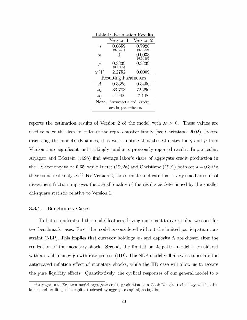
Table 1: Estimation ResultsVersion 1 Version 2

η 0.6659(0.1251)

0.7926(0.1339)

κ 0 0.0033(0.0018)

ρ 0.3339(0.0605)

0.3339

χ (1) 2.2752 0.0009Resulting Parameters

A 0.3388 0.3400φh 33.783 72.296φf 4.942 7.448Note: Asymptotic std. errors

are in parentheses.

reports the estimation results of Version 2 of the model with κ > 0. These values are

used to solve the decision rules of the representative family (see Christiano, 2002). Before

discussing the model’s dynamics, it is worth noting that the estimates for η and ρ from

Version 1 are significant and strikingly similar to previously reported results. In particular,

Aiyagari and Eckstein (1996) find average labor’s share of aggregate credit production in

the US economy to be 0.65, while Fuerst (1992a) and Christiano (1991) both set ρ = 0.32 in

their numerical analyses.13 For Version 2, the estimates indicate that a very small amount of

investment friction improves the overall quality of the results as determined by the smaller

chi-square statistic relative to Version 1.

3.3.1. Benchmark Cases

To better understand the model features driving our quantitative results, we consider

two benchmark cases. First, the model is considered without the limited participation con-

straint (NLP). This implies that currency holdings mt and deposits dt are chosen after the

realization of the monetary shock. Second, the limited participation model is considered

with an i.i.d. money growth rate process (IID). The NLP model will allow us to isolate the

anticipated inflation effect of monetary shocks, while the IID case will allow us to isolate

the pure liquidity effects. Quantitatively, the cyclical responses of our general model to a

13Aiyagari and Eckstein model aggregate credit production as a Cobb-Douglas technology which takeslabor, and credit specific capital (indexed by aggregate capital) as inputs.

20

persistent monetary shock will embody both of these effects.

The impulse responses to a one percent monetary tightening for the NLP model in pe-

riod t = 2 are illustrated in Figure 4.14 All nominal variables have been normalized by

the end-of-period base money supply. For NLP, as cash reserves are drained from interme-

diaries, household deposits respond positively to equate the marginal value of cash across

the goods and financial markets. The nominal interest rate follows Fisherian fundamentals

and declines from the anticipated deflation effect. The decline in the aggregate price level

indicates an increase in real balances. The decrease in the real cost of cash transactions

decreases household demand for credit services and the additional non-durable consumption

and household investment expenditures is financed with the increase in currency and deposit

usage. Employment in goods production and aggregate output rises. Finally, notice that

this version of the model predicts a negative co-movement between business and household

investment. That is, business investment expenditures are crowded out by the additional

spending on both household investment and non-durable consumption.15 While household

investment is procyclical, the model fails to capture the dynamic correlations between the

two investment series and has counterfactual predictions for the co-movement between M1

and nominal interest rates, non-durable consumption and real output.

The impulse response plots for the IID model are given in Figure 5.16 The liquidity effect

drains cash reserves and nominal rates rise, M1 declines in the period of the shock, and there

is a decline in output. There is a disproportionate increase in the relative price of house-

hold credit services and a substitution away from household credit production and towards

firm credit production. Household consumption of non-durables and durable investment

declines while business investment rises in the period of the shock. Hence the IID case of our

model reaches an opposite conclusion regarding the cyclical behavior of the two investments

compared to NLP. That is, while there continues to be a negative co-movement between

household and business investment, business investment is now countercyclical. Most of the

14The NLP model uses the parameter estimates reported for version 1 of the model. The NLP model wasattempted to be estimated separately, but this attempt failed because the counterfactual movement of theinvestment series (see Figure 4) cannot be corrected by varying the estimated variables.

15This feature can also be seen from the efficiency condition for business investment in Equation (19)which embodies an inverse relationship between consumption growth (i.e. the real interest rate) and firmcapital accumulation along the optimal path.

16Similar to the NLP analysis, the Version 1 estimate of η was used (see previous footnote).

21

2 4 6 8−0.1

0

0.1

Quarters

Investment

Household

Business

2 4 6 8

0

5

10

x 10−3

Quarters

Output

2 4 6 8

0

2

4

x 10−4

Quarters

Non−durable Cons.

2 4 6 8

−0.4

−0.2

0

Quarters

Price Level

2 4 6 8

−8

−6

−4

−2

x 10−4

Quarters

Nom. Interest Rate

2 4 6 8

−0.4

−0.2

0

Quarters

M1

2 4 6 80

0.2

0.4

Quarters

Deposits

2 4 6 8

−10

−5

0

x 10−3

Quarters

Crit. j*

2 4 6 8

−0.2

−0.1

0

Quarters

Pft/P

t

2 4 6 8−2

−1

0

Quarters

Pht

/Pt

2 4 6 8

−0.1

−0.05

0

Quarters

qft

2 4 6 8

−2

−1

0

Quarters

qht

Figure 4: Impulse responses from a negative monetary shock; without limited participationassumption. Y-axis denote percentage change from steady state.

22

2 4 6 8 10−1.5

−1

−0.5

0

Quarters

Investment

Household

Business

2 4 6 8 10

−0.2

−0.1

0

Quarters

Output

2 4 6 8 10

−8

−6

−4

−2

0x 10

−3

Quarters

Non−durable Cons.

2 4 6 8 10

−0.3

−0.2

−0.1

0

Quarters

Price Level

2 4 6 8 100

2

4

6

x 10−3

Quarters

Nom. Interest Rate

2 4 6 8 10

−1

−0.5

0

Quarters

M1

2 4 6 8 100

0.02

0.04

0.06

Quarters

Deposits

2 4 6 8 10

0

0.05

0.1

0.15

Quarters

Crit. j*

2 4 6 8 100

0.5

1

1.5

Quarters

Pft/P

t

2 4 6 8 100

5

10

Quarters

Pht

/Pt

2 4 6 8 10

0

0.1

0.2

Quarters

qft

2 4 6 8 10

−4

−2

0

Quarters

qht

Figure 5: Impulse responses from an iid negative monetary shock. Y-axis denote percentagechange from steady state.

real effects of the negative monetary innovation dissipates in the period following the shock

as household deposits are adjust to the unanticipated shock.

3.3.2. The General Case

The previous exercises illustrated that a monetary contraction that creates either an

anticipated deflation effect or a liquidity effect is unable to account for the real or mone-

tary facts regarding the two investment series. We now return to our general model and

investigate whether the interaction between limited participation and a persistent monetary

innovation can improve the model’s predictions. Impulse responses to a one percent mone-

tary tightening for versions 1 and 2 of the model are illustrated in Figures 6 and 7. With

the exception of firm credit production and business investment, the responses qualitatively

resemble the IID case in the period of the shock. Again, the monetary tightening at period

23

t = 2 immediately drains cash reserves from financial intermediaries and we see an imme-

diate decline in M1. The negative liquidity effect drives nominal rates are driven upwards

and the resulting contraction in the supply of credit increases in the relative prices of credit

services. This leads to a decline in the quantity of both household and firm credit services,

qhand qf . As consumer durables can only be financed with deposits and household credit,

constraint (14) implies that the decline in qh must be associated with a decrease in both non-

durable and durable consumption and constraint (13) states that a greater portion of real

non-durable consumption will be financed with cash. As business investment also responds

negatively to the higher price of firm credit, there is a positive co-movement between the two

investments. Furthermore, similar to the IID case, there is again a disproportionate impact

on the relative price of household credit, the decline in household investment exceeds that

of business investment. The decline in overall output indicates their procyclical behavior.17

In the period after the shock, household deposits increase and the anticipated deflation

effect drives the nominal interest rate and the relative price of credit below their steady

state values. M1, the normalized price level, and household credit production all move back

towards steady state. Subsequent movements in output, employment in goods production,

the nominal rate, the relative price of credit, and the two investment series resemble those

in the NLP model (see Figure 4). This is not surprising as the liquidity effect is only present

in the initial period of the shock. The exceptions are household credit production which

continues to rise, and non-durable consumption which continues to fall. Note that contrary

to what happens in NLP, household deposits and M1 both increase in the period after the

shock. This reinforces the increased availability of loanable funds to credit producers and

goes disproportionately to household credit production. The boom in household investment

is financed with the additional credit services and deposits at the expense of slightly less non-

durable consumption.18 Hence the economy’s investment resources shift towards household

investment and business capital is crowded-out. This negative co-movement between the

17As the increase in the relative price of household credit services exceeds that of firm credit, the modeldisplays a sharper decline in household investment consistent with Figure 1. The effect of increases in themarginal cost of household investment relative to firm investment can be seen in equations (18) and (19).

18The reallocation of deposits to finance household investment can be seen by noting that in the periodafter the shock, household investment rises above steady state while non-durable consumption continues todecline and household credit production remains below steady state.

24

2 4 6 8−0.3

−0.2

−0.1

0

0.1

Quarters

Household Inv. (χ = 0)

Household Inv. (χ > 0)

Business Inv. (χ = 0)

Business Inv. (χ > 0)

Figure 6: Impulse response to a negative monetary shock; limited participation. Y-axisdenotes percentage change from steady state. Version 1 of the model assumes κ = 0, whileVersion 2 of the model assumes κ > 0.

two investments in the period after the shock captures the protracted and lagged response

of business investment to household investment and M1 as in the data.

The impulse responses for Version 2 of the model with κ > 0 only change in two significant

ways relative to Version 1. First, there is more persistence in the investment series at the

expense of a smaller initial impact. This is also apparent in the behavior of labor hours

spent in credit production. Second, the large initial decline in durables investment incurs a

cost which alters the amount of wealth a household can devote to non-durable consumption,

resulting in a much sharper decline. Otherwise, the dynamic response to nominal interest

rates, deposits, M1, and all aggregate and relative prices show little quantitative changes

relative to Version 1.

25

2 4 6 8

−0.06

−0.04

−0.02

0

Quarters

Output

2 4 6 8

−2

−1

0x 10

−3

Quarters

Non−durable Cons.

2 4 6 8

−0.4

−0.2

0

Quarters

Price Level

2 4 6 8

0

5

10x 10

−4

Quarters

Nom. Interest Rate

2 4 6 8

−1

−0.5

0

Quarters

M1

2 4 6 80

0.05

0.1

0.15

Quarters

Deposits

2 4 6 80

0.1

0.2

Quarters

Crit. j*

2 4 6 8

0

0.1

0.2

Quarters

Pft/P

t

2 4 6 8

0

0.5

1

Quarters

Pht

/Pt

2 4 6 8

−0.03

−0.02

−0.01

0

Quarters

qft

2 4 6 8

−3

−2

−1

0

Quarters

qht

2 4 6 8

−0.1

−0.05

0

Quarters

n1t

χ=0

χ>0

Figure 7: Impulse response to a negative monetary shock; limited participation. Y-axisdenotes percentage change from steady state. Version 1 of the model assumes κ = 0, whileVersion 2 of the model assumes κ > 0.

26

3.4. Sensitivity Analysis

While the results presented above are fairly robust to deviations of the assumed pa-

rameter values and calibrating ratios prior to estimation, the calibration section noted the

importance of the reserve requirement ratio (θ) in obtaining a decline in non-durable con-

sumption at the onset of a monetary tightening. To show that the remaining results are not

sensitive to this parameter, Version 1 of the model was estimated with θ = 0.15 resulting in

η = 0.5833 (se = 0.1155) and ρ = 0.3735 (se = 0.0111) with χ (1) = 3.2628. This value for

θ is in line with average reserve holdings of the banking industry.19 The impulse responses

are presented in Figure 8. As the figure indicates, the only qualitative difference is that non-

durable consumption increases in response to a monetary contraction. The reason for this

result stems from the size of the deposit multiplier, 1/θ. The larger the deposit multiplier,

the larger the declines in M1 and the price level relative to the monetary base. These re-

sponses are illustrated in the middle row of the figure, with prices falling 23 percent and M1

falling 46 percent more than the benchmark results in Figure 7. This decline in prices allows

households to use their present money balances to increase their consumption of non-durable

goods. The value of θ used in the benchmark analysis suppresses this decline in prices and

M1, resulting in a decline in non-durable consumption. Nonetheless, the impulse responses

under both values illustrate similar qualitative responses to all other key variables, including

the investment paths.

4. Investment Responses to a Productivity Shock

While the goal of this paper is to investigate the behavior of investment components to a

monetary shock, it is of interest to evaluate how our credit and financial structure influences

the behavior of the model to a real productivity shock. This is achieved by restating the

production technology with an exogenous total factor productivity shock, Yt = ztkαt n

1−α1t ,

with zt = (1− 0.9) z̄ + 0.9zt−1 + εzt and z̄ = 1.

Using the previously estimated parameters from Table 1 (Version 1), the impulse re-

19Source: Federal Reserve Bulletin. 1997; the ratio of reserves to demand deposits is roughly 15 percentwhile the ratio of reserves to consumer and industrial loans is roughly 4 percent.

27

2 4 6 8 10

−0.04

−0.02

0

Quarters

Investment

Household

Business

2 4 6 8 10

−10

−5

0

x 10−3

Quarters

Output

2 4 6 8 10

0

1

2

x 10−3

Quarters

Non−durable Cons.

2 4 6 8 10

−0.6

−0.4

−0.2

0

Quarters

Price Level

2 4 6 8 10

0

5

10

x 10−4

Quarters

Nom. Interest Rate

2 4 6 8 10

−1.5

−1

−0.5

0

Quarters

M1

2 4 6 8 100

0.02

0.04

0.06

0.08

Quarters

Deposits

2 4 6 8 100

0.1

0.2

0.3

Quarters

Crit. j*

2 4 6 8 10

0

0.02

0.04

Quarters

Pft/P

t

2 4 6 8 10

−0.5

0

0.5

1

Quarters

Pht

/Pt

2 4 6 8 10

−8

−6

−4

−2

0

x 10−3

Quarters

qft

2 4 6 8 10

−3

−2

−1

0

Quarters

qht

Figure 8: Impulse response to a negative monetary shock with limited participation, κ = 0,and θ = 0.15. Y-axis denotes percentage change from steady state.

28

sponses to a one percent deviation to zt are illustrated in Figure 9.20 As the figure illustrates,

all real aggregates and real balances increase in response to a technology shock (as indicated

by the decrease in the normalized price level). The movement in our credit and financial

market variables arises from the resulting increase in the demand for loanable funds. These

include an increase in household deposits and household/firm credit services, used to finance

the additional household and business investment, and an increase in the nominal interest

rate and relative price of credit services. Note also that while the monetary base remains

constant, inside money and M1 increases. Hence, M1 will be procyclical and the financial

structure of our model also embodies a reverse causation explanation of the money-output

correlation. One of the more interesting results is that household and business investment

both increase at the impact of a shock and have a maximum, contemporaneous correlation

of 0.7933. While being far from our goal, this contemporaneous correlation is the primary

result of Gomme et al. (2001), and their stated improvement over the results of Benhabib

et al. (1991). While their results hinged on a time-to-build technology for physical capital

production relative to household durables, the model in this analysis captures this result as

a consequence of the representative family having more wealth to simultaneously devote to

both types of investment.

5. Conclusion

This paper accounts for the dynamic relationships between household investment, busi-

ness investment, broad monetary aggregates, and credit in a model of the monetary trans-

mission mechanism which highlights the interaction between financial intermediaries and the

credit market. The channel by which a negative monetary innovation leads to our quanti-

tative predictions relies on the differential impact of the resulting liquidity and anticipated

deflation effects on the price of household relative to firm credit services and their respective

investment expenditures. Such a path was generated in the absence of ex-ante constraints

regarding the timing of business and household investment. Furthermore, since monetary

20Re-estimating the model parameters for this exercise is not an option considering the data momentsused were specifically concerning a response to a monetary shock.

29

2 4 6 8 100

2

4

Quarters

Investment

Household

Business

2 4 6 8 100

0.5

1

Quarters

Output

2 4 6 8 100

0.2

0.4

Quarters

Non−durable Cons.

2 4 6 8 10

−0.6

−0.4

−0.2

0

Quarters

Price Level

2 4 6 8 100

2

4

x 10−3

Quarters

Nom. Interest Rate

2 4 6 8 100

1

2

3

Quarters

M1

2 4 6 8 100

2

4

Quarters

Deposits

2 4 6 8 10

−1.5

−1

−0.5

0

Quarters

Crit. j*

2 4 6 8 100

1

2

3

Quarters

Pft/P

t

2 4 6 8 100

5

10

Quarters

Pht

/Pt

2 4 6 8 100

2

4

Quarters

qft

2 4 6 8 100

2

4

Quarters

qht

Figure 9: Impulse response to a one percent productivity shock with κ = 0.Y-axis denotespercentage deviations from steady state.

30

injections effect the ability of the financial intermediaries to create deposits and issue loans,

movements in broad monetary aggregates such as M1 move with household investment and

are magnified beyond movements in the monetary base, as in the data.

While the benchmark results share many quantitative and qualitative features of the data

in response to a monetary shock, one limitation of the model is its inability to display the

observed degree of persistence. Christiano et al. (2005) conclude that model features such as

nominal wage and price rigidity, habit persistence, and others combined with real frictions

are necessary to observe a persistent response to a monetary shock. While including these

features would help deliver persistence, it would do so at a cost of complicating the model.

The goal of this paper was to present a model which captures the observed movements

in business investment, household investment, broad monetary aggregates, and credit in a

parsimonious framework without having to resort to these exogenous frictions. It is believed

that adding these numerous features will only improve the empirical results of the model,

and this is left for future work.

Appendices

VAR Analysis

Impulse responses were calculated by replicating the VAR estimation exercise of Chris-

tiano et al. (1999 and 2005). The variables were ordered in the VAR as Yt, Pt, PCOMt, HIt,

BIt, HCREDt, FFt, TRt, NBRt, and Mt and denote the log of real GDP, the log of the

implicit GDP deflator, the smoothed change in an index of sensitive commodity prices, the

log of real household investment, the log of real business investment, the log of the change

in household credit outstanding, the Federal Funds rate, the log of total reserves, the log of

nonborrowed reserves, and the log of M1, respectively. All data definitions and construction

are reported in the following appendix. The VAR includes four lagged values of each variable

and assumes a standard, recursive identification scheme. The 90 percent confidence intervals

displayed in the figures were calculated using the bootstrap method.

31

Data Appendix

Data used for the VAR analysis described above were defined and constructed as fol-

lows. Output was taken to be Gross Domestic Product (series name: GDP.US). Business

investment was taken to be the sum of nonresidential, fixed investment on structures (series

name: IFNS.US) and nonresidential, fixed investment on equipment and software (series

name: IFNES.US). Household investment was taken to be the sum of personal consump-

tion expenditures for durable goods (series name: CD.US) and residential, fixed investment

(series name: IFR.US). All nominal data was transformed to real by dividing them by the

GDP Implicit Price Deflator (series name: GDPDEF). Household credit was taken to be the

change in household credit market debt outstanding (series name: CMDEBT). The commod-

ity price index was taken to be the producer price index of industrial commodities (series

name: PPIIDC). The data for the Federal Funds rate, total reserves, nonborrowed reserves,

and M1 have series names RFED.US, TRARR, BOGNONBR, and M1.US, respectively. All

monthly data was made available by taking quarterly averages. The data sample is from

1959:1 to 2004:4 and is available from either the US Department of Commerce: Bureau of

Economic Analysis (BEA) or the Board of Governors from the Federal Reserve System.

32

References

[1] Aiyagari, S. R. and Eckstein, Z., “Interpreting Monetary Stabilization in a GrowthModel with Credit Goods Production,” in Financial Factors in Economic Stabilizationand Growth (Cambridge, MA: Cambridge University Press, 1996).

[2] Balke, N.S. and Wynne, M.A., “An Equilibrium Analysis of Relative Price Changes andAggregate Inflation,” Journal of Monetary Economics 45(1) (February 2000), 269-292.

[3] Benhabib, J., Rogerson, R. and Wright, R., “Homework in Macroeconomics: Householdproduction and Aggregate Fluctuations,” Journal of Political Economy 99(6) (December1991), 1166-1187.

[4] Bernanke, B. and Gertler, M., “Inside the Black Box: The Credit Channel of MonetaryPolicy Transmission,” Journal of Economic Perspectives 9(4) (Fall 1995), 27-48.

[5] Chang, C-Y, and Li, V.E., “The Cyclical Behavior of Household and Business Invest-ment in a Cash-in-advance Economy,” Journal of Economic Dynamics and Control 28(4)(January 2004), 691-706.

[6] Chari, V.V., Christiano, L.J. and Eichenbaum, M., “Inside Money, Outside Money, andShort-Term Interest Rates,” Journal of Money, Credit, and Banking 27(4) (November1995), 1355-1385.

[7] Christiano, L.J., “Modeling the Liquidity Effect of a Monetary Shock,” Federal ReserveBank of Minneapolis Quarterly Review 15(1) (Winter 1991), 3-34.

[8] Christiano, L.J. and Eichenbaum, M., “Liquidity Effects, Monetary Policy, and theBusiness Cycle,” Journal of Money, Credit, and Banking 27(4) (November 1995), 1113-1136.

[9] Christiano, L.J., Eichenbaum, M., and Evans, C., “Monetary Policy Shocks: What HaveWe Learned and to What End?” in J.B. Taylor and M. Woodford, eds., Handbook ofMacroeconomics, Amsterdamn: North Holland Press, 1999.

[10] Christiano, L.J. and Todd, R. M., “Time to Plan and Aggregate Fluctuations,” FederalReserve Bank of Mineapolis Quarterly Review 20(1) (Winter 1996), 14-27.

[11] Christiano, L.J., “Solving Dynamic Equilibrium Models by a Method of UndeterminedCoefficients,” Computational Economics 20(1-2) (October 2002), 21-55.

[12] Christiano, L.J., Eichenbaum, M., and Evans, C., “Nominal Rigidities and the DynamicEffects of a Monetary Policy Shock,” Journal of Political Economy 113(1) (February2005), 1-45.

[13] Cooley, T.F. and Hansen, G.D., “The Inflation Tax in a Real Business Cycle Model,”American Economic Review 79(4) (September 1989), 733-748.

[14] Cooley, T.F. and Hansen, G.D., “The Welfare Cost of Moderate Inflations,” Journal ofMoney, Credit, and Banking 23(3) (August 1991), 483-503.

33

[15] Diaz-Gimenez, J., Prescott, E.C., Fitzgerald, T., and Alvarez, F., “Banking in Com-putable General EquilibriumModels,” Journal of Economic Dynamics and Control 16(3-4) (July-October 1992), 533-339.

[16] Dressler, S.J., “The Cyclical Effects of Monetary Policy Regimes,” forthcoming in theInternational Economic Review (2006).

[17] Federal Reserve Bulletin, Board of Governors of the Federal Reserve System, Washing-ton, DC, 76(1990), A22.

[18] Fisher, J., “Relative Prices, Complementarities, and Co-Movement Among Componentsof Aggregate Expenditures,” Journal of Monetary Economics 39(3) (August 1997), 449-474.

[19] Fisher, J., “Why Does Household Investment Lead Business Investment over the Busi-ness Cycle?” Federal Reserve Bank of Chicago Working Paper WP2001-14 (2006).

[20] Freeman, S. and Kydland, F.E., “Monetary Aggregates and Output,” AmericanEconomic Review 90(5) (December 2000), 1125-1135.

[21] Fuerst, T.S., “Liquidity, Loanable Funds, and Real Activity,” Journal of MonetaryEconomics 29(1) (February 1992a), 3-24.

[22] Gertler, M. and Gilchrist, S., “The Role of Credit Market Imperfections in the Mon-etary Transmission Mechanism: Arguments and Evidence,” Scandinavian Journal ofEconomics 95(1) (1995), 43-64.

[23] Ghez, G.R. and Becker, G.S., The Allocation of Time and Goods over the Life Cycle,(New York: Columbia University Press, 1975).

[24] Gomme, P., Kydland, F.E., and Rupert, P.C., “Home Production Meets Time to Build,”Journal of Political Economy 109(5) (October 2001), 1115-1131.

[25] Greenwood, J., and Hercowitz, Z., “The Allocation of Capital and Time over theBusiness-Cycle,” Journal of Political Economy 99(6) (December 1991), 1188-1214.

[26] Hansen, L.P. and Singleton, K.J., “Stochastic Consumption, Risk Aversion, and theTemporal Behavior of Asset Returns," Journal of Political Economy 91(2) (April 1983),249-265.

[27] Kydland, F.E., and Prescott, E.C., “Business Cycles: Real Facts and a MonetaryMyth,” Federal Reserve Bank of Minneapolis Quarterly Review 14(2) (Spring 1990),3-18.

[28] Lee, B-S and Ingram, M.B.F., “Simulation Estimation of Time-Series Models,” Journalof Econometrics 47(2-3) (February-March 1991), 197-205.

[29] Li, V.E., “Household Credit and the Monetary Transmission Mechanism,” Journal ofMoney, Credit, and Banking 32(3) (August 2000), 335-356.

34

[30] Lucas Jr., R.E., “Liquidity and Interest Rates,” Journal of Economic Theory 50(2)(April 1990), 237-264.

[31] Newey, W.K. and West, K.D., “A Simple, Positive, Semi-Definite, Heteroskedasticityand Autocorrelation Consistent Covariance Matrix,” Econometrica 55(3) (May 1987),703-708.

[32] Porter, R.D. and Judson, R.A., “The Location of US Currency: How Much is Abroad?”Federal Reserve Bulletin 82(10) (1996), 883-903.

35