IZA DP No. 1344

Input versus Output Taxation in anExperimental International Economy

Arno RiedlFrans van Winden

DI

SC

US

SI

ON

PA

PE

R S

ER

IE

S

Forschungsinstitutzur Zukunft der ArbeitInstitute for the Studyof Labor

October 2004

Input versus Output Taxation in an Experimental International Economy

Arno Riedl CREED, University of Amsterdam, Tinbergen Institute and IZA Bonn

Frans van Winden

CREED, University of Amsterdam and Tinbergen Institute

Discussion Paper No. 1344 October 2004

IZA

P.O. Box 7240 53072 Bonn

Germany

Phone: +49-228-3894-0 Fax: +49-228-3894-180

Email: iza@iza.org

Any opinions expressed here are those of the author(s) and not those of the institute. Research disseminated by IZA may include views on policy, but the institute itself takes no institutional policy positions. The Institute for the Study of Labor (IZA) in Bonn is a local and virtual international research center and a place of communication between science, politics and business. IZA is an independent nonprofit company supported by Deutsche Post World Net. The center is associated with the University of Bonn and offers a stimulating research environment through its research networks, research support, and visitors and doctoral programs. IZA engages in (i) original and internationally competitive research in all fields of labor economics, (ii) development of policy concepts, and (iii) dissemination of research results and concepts to the interested public. IZA Discussion Papers often represent preliminary work and are circulated to encourage discussion. Citation of such a paper should account for its provisional character. A revised version may be available directly from the author.

IZA Discussion Paper No. 1344 October 2004

ABSTRACT

Input versus Output Taxation in an Experimental International Economy∗

This paper is concerned with a policy oriented macroeconomic experiment involving an 'international' economy with a relatively small 'home' country and a large 'foreign' country. It compares the economic performance of two alternative tax systems as a means to finance unemployment benefits: a sales-tax-cum-labor-subsidy system versus a wage tax system. The two systems are applied to the home country, while the wage tax system always obtains in the foreign country. In stark contrast with expectations of experts the sales tax system clearly outperforms the wage tax system, using standard economic indicators. It is argued that producers' reluctance to incur costs up-front while being uncertain about product prices can explain this outcome. Several pieces of evidence are provided to support this claim. The results strongly suggest that behavioral aspects have to be taken into account also in applied macroeconomic models. JEL Classification: A10, C90, C91, D21, D80, E62, H20 Keywords: laboratory experiment, wage tax, sales tax, macroeconomic policy, behavioral

economics Corresponding author: Arno Riedl CREED University of Amsterdam Roetersstraat 11 1018 WB Amsterdam The Netherlands Email: a.m.riedl@uva.nl

∗ This paper uses data generated by a research project commissioned by the Dutch Ministry of Social Affairs and Employment, see van Winden, Riedl, Wit, and van Dijk (1999). Financial support by the Ministry and comments and suggestions by its Steering Committee are gratefully acknowledged. We would like to thank Frans van Dijk and Jörgen Wit who were both involved in the experimental design of the project, and, in addition, Jörgen Wit for the computation of the equilibria of the theoretical model used. Our gratitude also goes to Jos Theelen for the development of the excellent software used in the experiment, and to G. Cotteleer, J.H.H. Notmijer, and M. Smits for their assistance in running the experiments. Former versions of this paper have been presented at conferences, workshops and seminars in Amsterdam, Barcelona, Bari, Berlin, Bonn, Frankfurt, Groningen, Lake Tahoe, Munich, New York, Rhodos, St. Gallen, The Hague, Tilburg, Venice, Zurich. We thank the participants for their helpful remarks. We are in particular grateful to Kurt Hildenbrand, Ruud de Mooij, Charles Noussair, Raymond Riezman, Shyam Sunder, and Claus Weddepohl for their valuable comments. This paper is part of the EU-TMR Research Network ENDEAR (FMRX-CT-98-0238). The usual disclaimer applies.

1 Introduction

Time usually elapses (...) between the incurring of costs by the producer

(with the consumer in view) and the purchase of the output by the ultimate

consumer. Meanwhile the entrepreneur (...) has to form the best expecta-

tions he can as to what the consumers will be prepared to pay when he is

ready to supply them (...).

John Maynard Keynes (1970 [1936], Ch. 5: Expectation as Determining

Output and Employment, p. 46)

A major economic issue concerns the effects of taxation on the behavior of individual

consumers and producers and the performance of markets. In this context, a longstand-

ing problem in public finance relates to the pros and cons of taxing inputs, e.g. labor

and capital, versus the taxation of outputs, like sales or value added. One potentially

highly relevant factor in this respect is that production takes time, a fact emphasized by

Keynes in the preceding quote. At the time when producers have to make their input

decisions, generally, the precise market conditions prevailing at the time consumers buy

their products are unknown. Thus, when deciding on labor and capital employment

producers, typically, face uncertainty about the real returns from these decisions. A

similar problem holds for consumers when they have to allocate time between labor

and leisure, because the real return on their labor will depend on the development of

consumer prices over the period covered by the wage contract.

Several studies have argued that taking this uncertainty into account is important

from a behavioral explanatory and optimal policy point of view. For example, Eaton

and Rosen (1980) show that if consumers are uncertain about the real wage, an ex-

pected income-compensated increase in the wage tax may induce them to supply more

labor. Moreover, lump-sum taxation is no longer necessarily efficient, because the wage

tax insures the consumer against random real wage income movements. Regarding pro-

ducers, a number of theoretical partial equilibrium studies have focused on the effects

of output price uncertainty on the input and supply decisions of firms. Results show

that output price uncertainty generally reduces factor demand and production level

of risk-averse competitive firms (Sandmo 1971, Batra and Ullah 1974, Hartman 1975,

1976, Holthausen 1976, Ghosal 1995).1

1Loss aversion, as in prospect theory (Kahneman and Tversky 1979), would seem to make this effect

1

The policy relevance of this topic can be illustrated by referring to “the puzzle of

European unemployment” (Blanchard and Katz (1997)). A large piece of this puzzle

seems related to the strong reliance on wage taxation in financing the welfare state, and

the focus on supply side conditions in employment policies. Indeed, several scholars

have pointed at the pernicious effects of wage taxation in this respect, with rising tax

rates and unemployment leading to a vicious circle (Snower (2000)). These arguments

and the above mentioned research suggests that shifting taxation from inputs to outputs

may have a positive effect on production and employment because the government then

effectively shares the sales risk faced by producers.

From an optimal taxation and general equilibrium perspective, however, it seems

not at all clear whether such a shift in taxation will do any good, in particular in a small

open economy. Taxation of outputs implies an implicit tax on the mobile factor capital

and the conventional wisdom in the literature on optimal taxation in open economies

is that taxing such a factor should be avoided. For example, based on the seminal work

of Diamond and Mirrlees (1971), Razin and Sadka (1991) have shown that a small

open economy should not tax mobile capital (at the source). More recently, Bovenberg

(1994, p. 284) argued that “(...) small and open economies should not tax highly mobile

factors (...)”.2

On the other hand, pure theoretical reasoning does not always provide unambiguous

answers, even in a frictionless perfectly competitive world. A well-known result from

general equilibrium theory is that, generically, equilibrium predictions are not unique.

In case of multiple equilibria, however, no clear forecasts concerning policy reforms can

be made. A main motivation of this paper is, therefore, to shed some light on this

thorny issue of whether a tax on immobile labor or a sales taxes - implicitly taxing

mobile capital - leads to a better economic performance of a small open economy. In

fact, in the framework we will be using theoretically multiple equilibria arise.

only stronger. Another strand of literature addresses the impact of (macroeconomic) uncertainty on

investment, typically showing a negative effect (Aizenman and Marion 1993, Brunetti and Weder 1998,

Guiso and Parigi 1999).

2Many relatively small countries nevertheless tax capital implicitly or explicitly. A large body of

literature tries to square this empirical fact with the theory of optimal taxation either by discussing

legal details (e.g. Gordon 1992), allowing for frictions and market imperfections (e.g. Richter and

Schneider 2001, Koskela and Schob 2002) or taking a global view of capital taxation (Braulke and

Corneo 2003).

2

Another motivation relates to the novelty of the research method. For our inves-

tigation we use data from an experimental study pitting a wage tax system against a

sales tax system as alternative means to finance unemployment benefits, commissioned

by the Dutch Ministry of Social Affairs and Employment.3 The Minister was requested

to do so in a motion carried by the Second Chamber of the Dutch parliament. To

our knowledge, it is for the first time that policymakers explicitly asked for laboratory

experimentation as a means to advise in macroeconomic policymaking. When doing

our investigation we were supervised by a steering committee to which internationally

renowned Dutch economists (in the fields of public economics, labor economics, exper-

imental economics and applied general equilibrium modeling) were assigned.4 Being a

policy-oriented study, the experimental design was required to show some parallelism

with the Dutch economy. The steering committee had to approve the design of the

experiment and assist the project.

Further innovative aspects of our study concern the comparison of different tax

systems in a macroeconomic experiment, and the implementation of a relatively small

‘home’ economy and a large ‘foreign’ economy in the laboratory.5 In a sense, doing

this study meant exploring the boundaries of the research method of laboratory ex-

perimentation. In our view, the results show that also in this area of policy related

macroeconomic research experiments are a useful complementary research tool, next

to theoretical and field empirical analyses. Compared to field econometric studies an

important advantage is that it is possible to empirically analyze the economic conse-

quences of a complete implementation of a new tax system. With the additional virtue

of being able to do so in a controlled way. Furthermore, an experiment offers the op-

portunity to generate (and if necessary replicate) the micro-level data of interest and

3See van Winden, Riedl, Wit, and van Dijk (1999).

4For economically intuitive reasons, backed by the above mentioned theoretical results from optimal

taxation theory, the members of the committee had the general opinion that the sales tax system

would lead to capital flight, more unemployment, and a substantial welfare loss in a relatively small

open economy, like The Netherlands. In addition, it was feared that a shift in economic activity would

take place from the relatively capital intensive ‘exposed sector’ (producing tradeable goods) towards

the more labor intensive ‘sheltered sector’. The more so, because high tax rates were foreseen due to

a labor subsidy that was incorporated in the alternative sales tax system.

5Akerlof (2002) discusses some other recent experiments related to macroeconomic issues.

3

avoids the noise field data are unavoidably exposed to.6 In addition, no specific behav-

ioral assumptions are needed, nor a restriction to a partial equilibrium framework as

in the theoretical studies referred to above. Moreover, since theory generically predicts

multiple equilibria, experiments can provide information on their relative attractiveness

in practice; an issue that will also prominently show up in our study.

More specifically, the experimental international economy that we will investigate

consists of two ‘countries’, one of which - the home country - is relatively small in terms

of potential economic activity. In each country consumers and producers are active.

Consumers supply labor and capital to producers on local and global input markets.

In both countries, producers are distributed over two production sectors: a sheltered

sector producing a relatively labor intensive commodity for a local output market, and

an exposed sector producing a relatively capital intensive commodity for a global output

market. All production factors and consumption goods are traded through multi-unit

double auctions.7 In the benchmark experimental treatment, in both countries, a wage

tax finances the benefits consumers receive for unemployed labor. In the alternative

treatment, the wage tax system is substituted by a sales tax system, in the home

country only. Under this system, instead of having to pay a tax on labor up-front, a

producer is taxed according to the proceeds from sales. Moreover, for each employed

unit of labor the producer receives a subsidy equal to the unemployment benefit.

The theoretical general equilibrium predictions turn out to be unique for the wage

tax system. For the alternative sales-tax-cum-labor-subsidy system, however, we obtain

two stable general equilibria implying two quite distinct sets of theoretical predictions

concerning the economic performance indicators of this system. One set of predictions

supports the economically intuitive hypothesis of capital flight from the small to the

large country with very negative effects on factor employment, production, consumption

and, hence, welfare in the small country. In the second equilibrium, however, almost

no capital flight occurs and labor employment, production, and consumption levels are

even higher than under the benchmark system. The experiment allows us to investigate

whether economic activities are attracted to one of these equilibria.

6In empirical studies of taxation this is a notorious problem which, for example, manifests itself in

widely diverging estimates of tax rate elasticities (see e.g. Sørensen (1997)).

7Double auctions are typically used for their capability to facilitate the equilibration of supply and

demand and the generation of efficient outcomes (see e.g. Davis and Holt (1993)).

4

To evaluate the performance of the two tax systems relative to each other as well as

relative to the theoretical predictions we mainly use the following economic indicators:

employment of labor, capital flight, shift towards labor intensive production, real GDP,

consumer earnings, and the budget surplus. Our main findings are the following. First,

despite of the rather complex experimental environment, we observe a clear tendency

towards equilibration of the economic process. Second, it turns out that the wage

tax system shows persistent budget deficits, while tax adjustments to balance these

deficits have a strong negative impact on the employment of labor and real GDP.

Third, shifting taxation from wages to sales and subsidizing labor in the home country

has substantial positive budgetary and real economic effects for this country. Moreover,

there is no evidence of capital flight nor of a shift in economic activity towards the labor

intensive sector. Fourth, under the alternative sales tax system economic behavior

tends to coordinate on the equilibrium with the higher activity level or performs even

better than this equilibrium predicts. In summary, the alternative sales-tax-cum-labor-

subsidy system performs significantly better than the wage tax system.

To explain these findings we claim that producers’ aversion towards incurring costs

up-front, while facing output price uncertainty, plays a crucial role. The sales-tax-cum-

labor-subsidy system is clearly much more producer and employment friendly in this

respect. Instead of having to pay a tax on the input of labor, a subsidy is received, while

through the sales tax the government is sharing the risk the producer runs with respect

to the return on output. We present theoretical arguments and empirical evidence to

support our claim.

Our results point at a hitherto underexposed behavioral regularity, with relevance

for economic model building as well as policy advising. Regarding the latter our study

fits into a still small but gradually growing stream of ‘design’ studies which involve the

economist as ‘engineer’ (Roth 2002). In these studies experimental and computational

economics are used as research methods filling the gap between theory and design.

For the development of theory these studies can be helpful by posing challenges and

suggesting some new answers to open questions. However, as Roth notes: “Whether

economists will often be in a position to give highly practical advice on design depends

in part on whether we report what we learn, and what we do, in sufficient detail to allow

scientific knowledge about design to accumulate” (ibid., p. 1342). With our paper we

hope to make a contribution to this empirical feedback mechanism.

5

The organization of the paper is as follows. Section 2 presents the experimental

design and procedures, as well as the theoretical predictions. The experimental results

are given in Section 3. In Section 4 we propose a behavioral explanation for our main

findings, while additional supportive evidence is provided. Section 5 concludes.

2 Experimental design

In the following, the wage tax system is denoted as the WT-system and the alternative

sales-tax-cum-labor-subsidy system as the STLS-system.

2.1 Economic Environment

In view of the desired parallelism with a relatively small open economy, we consider

an ‘international’ economy with consumers and producers in two ‘countries’, a rela-

tively small country s, the home country, and a large country l, the foreign country.

Consumers are endowed with units of capital (K) and labor (L) that they can sell to

producers in a capital and a labor market. Consumers derive utility from ‘leisure’, i.e.

unsold units of labor, and the consumption of two private goods: X and Y . In addi-

tion to factor payments, the consumption budget is determined by an unemployment

benefit for each unsold unit of labor. Commodities X and Y are produced in separate

sectors. Producers need capital and labor as inputs, which are transformed to outputs

via CES production technologies. The production of good X is relatively capital in-

tensive, while the production of Y is relative labor intensive. Profits are determined by

the difference between sales revenue and the costs of inputs. The former may involve

sales taxes and the latter wage taxes or labor subsidies, depending on the prevailing

tax system. Taxes are paid for the finance of unemployment benefits and/or labor

subsidies (see the next subsection). Both the capital market and the market for X are

international (exposed), while the markets for labor and good Y are local (sheltered).

Consequently, the total number of input and output markets equals six. Figure 1 shows

a flow diagram illustrating the economic environment.

Consumers are endowed with K units of capital and L units of labor. Preferences

over leisure (L − L) and the two consumption goods, X and Y , are induced by a log-

6

Consumers insmall country

Producers Y insmall country

Producers X insmall country

Producers X inlarge country

Producers Y inlarge country

Consumers inlarge country

'&

$%

Labor market insmall country

'&

$%

Market for Y insmall country

'&

$%

Internationalmarket for X

'&

$%

Market for Y inlarge country

'&

$%

Labor market inlarge country

'&

$%

Internationalcapital market

- - -

- - -

@@

@@

@@

@R

��

��

��

��

QQ

QQ

QQQs

��

��

���3

����1

PPPPq

��

��

��

��

��3

QQ

QQ

QQ

QQ

QQs

ZZ

ZZ~

��

��>

?

6

?

6

Figure 1 – Flow diagram of the economic environment

linearized Cobb-Douglas type of utility function.8 Producers are endowed with a CES

production technology exhibiting slightly decreasing returns to scale and allowing for

different factor intensities and elasticities of substitution in the two production sectors.9

In the upper part of Table 1 the continuous approximations of the discrete utility

(earnings) and output tables used in the experiments are shown. The rest of this table

will be discussed below.

All inputs and outputs are traded in computerized multiple units double auction

markets as introduced by Plott and Gray (1990). The choice of this market type is

guided by its reputation of fast equilibration of supply and demand in experimental

8The use of a log-linearized Cobb-Douglas utility function has the advantage that subjects could

be provided with a simple sheet of paper showing the marginal and total payoff for each of the three

arguments, even though three goods entered the utility function as variables.

9The actually implemented factor intensities and substitution elasticities resemble estimates for the

Dutch economy. The choice of slightly decreasing returns to scale is motivated by an empirical and

a methodological consideration. Firstly, empirical evidence exist supporting this choice (see Basu and

Fernald (1997)). Secondly, it allows experimental producers to make strictly positive profits, and hence

monetary earnings, in the theoretical general equilibrium discussed below.

7

Table 1 – Experimental parameters

Preferences and production technologies

Consumers i (utility functions):

Uik= 25

[

ln Xik+ ln Yik

+ .25 ln(Lik− Lik

)]

,

Uik= 0 if either Xik

, Yik, or Lik

− Likequals zero,

}

in both tax systems (k = s, l)

Quantities Lik, Yik

are determined ‘locally’ (within a country)

Quantities Xikare determined ‘internationally’ (one global market)

Producers j (production functions and profit functions):

Zjzk= Ak

[

η1−γzz Lγz

jzk+ (1 − ηz)

1−γz Kγz

jzk

] 0.9γz , Z = X, Y ; z = x, y; k = s, l

Labor intensities : ηx = .5625, ηy = .675; Substitution elasticities : γx = −2, γy = −6

Scaling factor: As = 1 (small country), Al = 1.21 (large country)

Πjxk= pxXjxk

− (1 + τwk)wkLjxk− rKjxk

,

Πjyk= pykYjyk

− (1 + τwk)wkLjyk− rKjyk

, k = s, l

}

in WT-system

Πjxs = (1 − τxs)pxXjxs − (ws − w0)Ljxs − rKjxs ,

Πjys = (1 − τys)pysYjys − (ws − w0)Ljys − rKjys ,

Πjxl= pxXjxl

− (1 + τwl)wlLjxl− rKjxl

,

Πjyl= pylYjyl

− (1 + τwl)wlLjyl− rKjyl

,

in STLS-system

Prices pyk, wk, taxes τwk, τzs, and quantities Ljzk, Yjyk

are determined ‘locally’

(within country k = s, l)

Prices px, r, and quantities Kjxk, Xjxk

are determined ‘internationally’

(one global market)

Endowments (both tax systems)

Small country Large country

Consumer Li = 15, Ki = 10, Cashi = 181 Li = 105, Ki = 70, Cashi = 1268

X-producer Lj = 0, Kj = 0, Cashj = 1223 Lj = 0, Kj = 0, Cashj = 8557

Y -producer Lj = 0, Kj = 0, Cashj = 815 Lj = 0, Kj = 0, Cashj = 5705

Number of agents

Consumers 3 3

X-Producers 2 2

Y -Producers 3 3

Tax systems

WT-system STLS-system

Both countries k Small country s Large country l

Unemployment benefit (w0) 70 70 70

Labor subsidy (w0) 0 70 0

Initial wage tax rate (τ0w) .3777 0 .3777

Wage tax τ t+1

wk wtkLt

k = τ t+1

wl wtkLt

l =

adjustment rule (τ t+1w ) w0(Lk − Lt

k) w0(Ll − Ltl)

Initial sales tax rate X (τ 0x) 0 .6521 0

Initial sales tax rate Y (τ0y ) 0 .7518 0

Sales taxes τ t+1xs pt

xXts + τ t+1

ys ptysY

ts = w0Ls

adjustment rule (τ t+1x , τ t+1

y ) τ t+1xs /τ t+1

ys = τ0xs/τ0

ys

Note: In the table describing the tax systems, t denotes a trading period, the variables Ltk, Lk, Xs, and Ys denote

aggregates in a country, superscripts 0 refer to initial values.

8

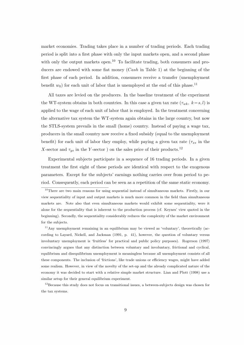
market economies. Trading takes place in a number of trading periods. Each trading

period is split into a first phase with only the input markets open, and a second phase

with only the output markets open.10 To facilitate trading, both consumers and pro-

ducers are endowed with some fiat money (Cash in Table 1) at the beginning of the

first phase of each period. In addition, consumers receive a transfer (unemployment

benefit w0) for each unit of labor that is unemployed at the end of this phase.11

All taxes are levied on the producers. In the baseline treatment of the experiment

the WT-system obtains in both countries. In this case a given tax rate (τwk, k=s, l) is

applied to the wage of each unit of labor that is employed. In the treatment concerning

the alternative tax system the WT-system again obtains in the large country, but now

the STLS-system prevails in the small (home) country. Instead of paying a wage tax,

producers in the small country now receive a fixed subsidy (equal to the unemployment

benefit) for each unit of labor they employ, while paying a given tax rate (τxs in the

X-sector and τys in the Y -sector ) on the sales price of their products.12

Experimental subjects participate in a sequence of 16 trading periods. In a given

treatment the first eight of these periods are identical with respect to the exogenous

parameters. Except for the subjects’ earnings nothing carries over from period to pe-

riod. Consequently, each period can be seen as a repetition of the same static economy.

10There are two main reasons for using sequential instead of simultaneous markets. Firstly, in our

view sequentiality of input and output markets is much more common in the field than simultaneous

markets are. Note also that even simultaneous markets would exhibit some sequentiality, were it

alone for the sequentiality that is inherent to the production process (cf. Keynes’ view quoted in the

beginning). Secondly, the sequentiality considerably reduces the complexity of the market environment

for the subjects.

11Any unemployment remaining in an equilibrium may be viewed as ‘voluntary’, theoretically (ac-

cording to Layard, Nickell, and Jackman (1991, p. 41), however, the question of voluntary versus

involuntary unemployment is ‘fruitless’ for practical and public policy purposes). Rogerson (1997)

convincingly argues that any distinction between voluntary and involuntary, frictional and cyclical,

equilibrium and disequilibrium unemployment is meaningless because all unemployment consists of all

these components. The inclusion of ‘frictions’, like trade unions or efficiency wages, might have added

some realism. However, in view of the novelty of the set-up and the already complicated nature of the

economy it was decided to start with a relative simple market structure. Lian and Plott (1998) use a

similar setup for their general equilibrium experiment.

12Because this study does not focus on transitional issues, a between-subjects design was chosen for

the tax systems.

9

In periods 9-16 tax rates are adjusted at the beginning of each new period such that

a balanced budget would be obtained for the previous period, given the market out-

comes of that period. The initial tax rates and the precise tax adjustment rules are

shown in the lower part of Table 1.13 This procedure guarantees a sufficient number

of repetitions with a constant environment for making it possible to examine whether

and at which level economic behavior stabilizes. The adjustment of the tax rates to

the budget balance adds an important feature of realism and enables an analysis of

the dynamic interaction between taxation, employment and other indicators of eco-

nomic performance, while keeping everything else constant. It also allows to control

for the potentially confounding effect that a relative good performance of a tax system

is ‘bought’ by budget deficits.

Table 1 shows the parameter values chosen for the endowments, utility functions,

production functions, and the number of agents. To implement a large country in the

laboratory the following solution was chosen. While keeping the number of consumers

and producers the same for both countries, consumers in the large country are endowed

with seven times as many units of labor and capital as holds for the consumers in the

small country (see the different L and K in the table). Moreover, the scaling factors

(As and Al) in the production functions are adjusted such that, theoretically, supply

and demand in the large economy are seven times as large as in the small economy, in

the baseline treatment with the WT-system (see next subsection).14

2.2 Theoretical General Equilibrium Predictions

Given the complex nature of the experimental economy, with several interdependent

markets and the double auction trading mechanism, the most natural solution concept

is the general equilibrium. We calculated the numerical solution(s) of a competitive

general equilibrium model equating supply and demand in the various markets with

13An upper bound of 0.90 was maintained for the tax rates because pilot studies showed that tax

rates too close to 100% might have a strongly discouraging effect on trading.

14The alternative approach of increasing the number of agents instead of endowments would not

have been feasible. With the requirement of at least three agents on each side of a market to ensure

competitiveness (see Davis and Holt (1993), Huck, Konrad, Muller, and Normann (2001)), the minimal

number of subjects per experimental session would have been 64, exceeding by far the capacity of the

laboratory.

10

the additional requirement of a balanced tax-transfer budget. We thereby follow other

studies of experimental markets using a similar procedure (see e.g. Noussair, Plott,

and Riezman (1995, 1997), Quirmbach, Swenson, and Vines (1996)).

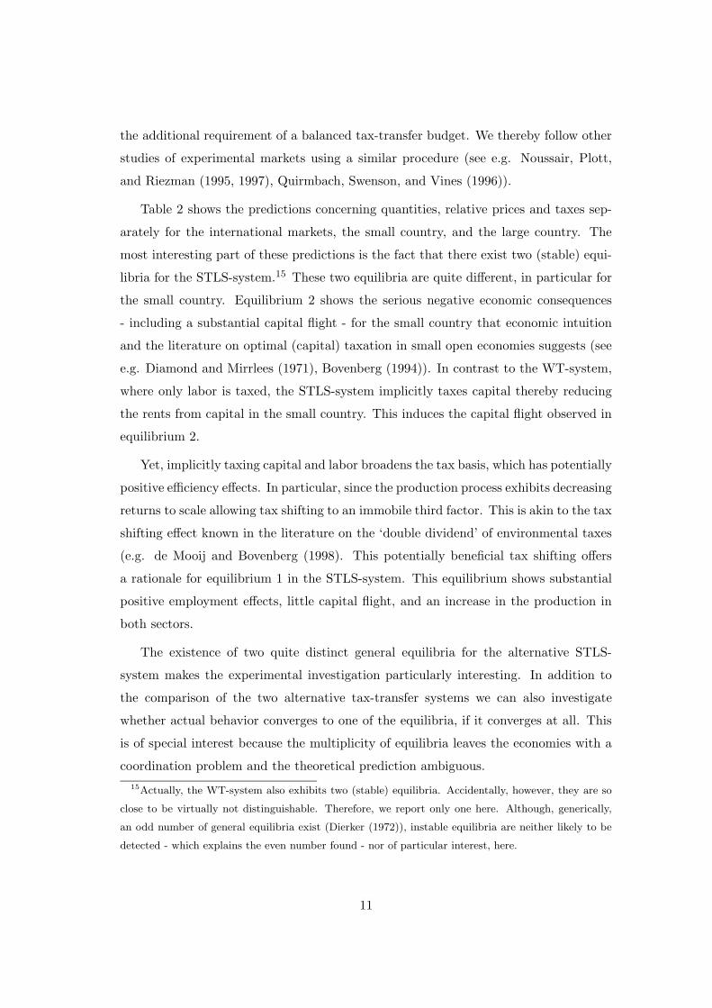
Table 2 shows the predictions concerning quantities, relative prices and taxes sep-

arately for the international markets, the small country, and the large country. The

most interesting part of these predictions is the fact that there exist two (stable) equi-

libria for the STLS-system.15 These two equilibria are quite different, in particular for

the small country. Equilibrium 2 shows the serious negative economic consequences

- including a substantial capital flight - for the small country that economic intuition

and the literature on optimal (capital) taxation in small open economies suggests (see

e.g. Diamond and Mirrlees (1971), Bovenberg (1994)). In contrast to the WT-system,

where only labor is taxed, the STLS-system implicitly taxes capital thereby reducing

the rents from capital in the small country. This induces the capital flight observed in

equilibrium 2.

Yet, implicitly taxing capital and labor broadens the tax basis, which has potentially

positive efficiency effects. In particular, since the production process exhibits decreasing

returns to scale allowing tax shifting to an immobile third factor. This is akin to the tax

shifting effect known in the literature on the ‘double dividend’ of environmental taxes

(e.g. de Mooij and Bovenberg (1998). This potentially beneficial tax shifting offers

a rationale for equilibrium 1 in the STLS-system. This equilibrium shows substantial

positive employment effects, little capital flight, and an increase in the production in

both sectors.

The existence of two quite distinct general equilibria for the alternative STLS-

system makes the experimental investigation particularly interesting. In addition to

the comparison of the two alternative tax-transfer systems we can also investigate

whether actual behavior converges to one of the equilibria, if it converges at all. This

is of special interest because the multiplicity of equilibria leaves the economies with a

coordination problem and the theoretical prediction ambiguous.

15Actually, the WT-system also exhibits two (stable) equilibria. Accidentally, however, they are so

close to be virtually not distinguishable. Therefore, we report only one here. Although, generically,

an odd number of general equilibria exist (Dierker (1972)), instable equilibria are neither likely to be

detected - which explains the even number found - nor of particular interest, here.

11

Table 2 – Theoretical general equilibrium predictions

WT-system STLS-system

equilibrium 1 equilibrium 2

International

K 240 240 240

X 177 181 182

r 0.0307 0.0295 0.0289

px 0.1882 0.1807 0.1807

Small country

Ks 30 28 11

Ls 28 33 18

Xcs 22 25 17

Xps 22 25 14

Ys 19 21 11

ws 0.1694 0.1971 0.1292

pys 0.2211 0.2165 0.2747

τws 0.3777

τxs 0.4889 0.7835

τys 0.5414 0.8677

Large country

Kl 210 212 229

Ll 197 199 213

Xcl 155 156 165

Xpl 155 156 168

Yl 132 133 140

wl 0.1694 0.1640 0.1743

pyl 0.2211 0.2123 0.2121

τwl 0.3777 0.3655 0.2769

Note: Equilibrium quantities are rounded to integers. De-

picted prices are relative prices that are obtained by divid-

ing nominal prices by the sum of all six nominal prices. The

equilibrium tax rates guarantee a balanced budget in equi-

librium. Superscript c (p) indicates consumed (produced)

quantities; when this distinction is not made consumed and

produced quantities coincide in equilibrium.

In order to avoid a potential bias of the experimental results in favor of the alter-

native tax system, and because the experiment was also policy oriented, it was decided

not to take the initial tax rates for the STLS-system from one of the two equilibria of

the theoretical model. Instead, these were determined such that on impact the produc-

ers of X and Y would have to bear the same tax burden as empirically observed (in

12

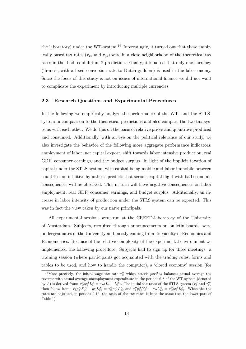
the laboratory) under the WT-system.16 Interestingly, it turned out that these empir-

ically based tax rates (τxs and τys) were in a close neighborhood of the theoretical tax

rates in the ‘bad’ equilibrium 2 prediction. Finally, it is noted that only one currency

(‘francs’, with a fixed conversion rate to Dutch guilders) is used in the lab economy.

Since the focus of this study is not on issues of international finance we did not want

to complicate the experiment by introducing multiple currencies.

2.3 Research Questions and Experimental Procedures

In the following we empirically analyze the performance of the WT- and the STLS-

system in comparison to the theoretical predictions and also compare the two tax sys-

tems with each other. We do this on the basis of relative prices and quantities produced

and consumed. Additionally, with an eye on the political relevance of our study, we

also investigate the behavior of the following more aggregate performance indicators:

employment of labor, net capital export, shift towards labor intensive production, real

GDP, consumer earnings, and the budget surplus. In light of the implicit taxation of

capital under the STLS-system, with capital being mobile and labor immobile between

countries, an intuitive hypothesis predicts that serious capital flight with bad economic

consequences will be observed. This in turn will have negative consequences on labor

employment, real GDP, consumer earnings, and budget surplus. Additionally, an in-

crease in labor intensity of production under the STLS system can be expected. This

was in fact the view taken by our naıve principals.

All experimental sessions were run at the CREED-laboratory of the University

of Amsterdam. Subjects, recruited through announcements on bulletin boards, were

undergraduates of the University and mostly coming from its Faculty of Economics and

Econometrics. Because of the relative complexity of the experimental environment we

implemented the following procedure. Subjects had to sign up for three meetings: a

training session (where participants got acquainted with the trading rules, forms and

tables to be used, and how to handle the computer), a ‘closed economy’ session (for

16More precisely, the initial wage tax rate τ 0w which ceteris paribus balances actual average tax

revenue with actual average unemployment expenditure in the periods 6-8 of the WT-system (denoted

by A) is derived from: τ0wwA

s LAs = w0(Ls − LA

s ). The initial tax rates of the STLS-system (τ 0x and τ0

y )

then follow from: τ0xpA

x XAs − w0L

Axs = τ0

wwAs LA

xs and τ0y pA

ysYA

s − w0LAys = τ0

wwAs LA

ys. When the tax

rates are adjusted, in periods 9-16, the ratio of the tax rates is kept the same (see the lower part of

Table 1).

13

getting subjects experienced with trading), and the international economy session.17

Subjects were paid out only at the end of the third meeting. They received a show-up

fee of 70 Dutch guilders for the training session. In the closed economy sessions they

earned on average 27 guilders, while receiving 40 guilders as a show-up fee. The show-up

fee for the international economy session was 10 guilders, while average earnings in this

sessions amounted to 120 guilders (at the time of the experiments one Dutch guilder

was worth approximately 0.52 U.S. dollar). All meetings lasted about 3.5 hours. At the

training session each subject was randomly assigned the role of consumer or producer,

which they kept in the subsequent meetings.

At the beginning of an experimental session subjects received instructions consist-

ing of a general part, read aloud by the experimenter, and a role-specific part, which

was quietly read by the subjects. They further received personal history forms with

all the information that was relevant to them (concerning endowments, markets they

were allowed to trade in, any taxes or subsidies, and the conversion rate of ‘francs’

to guilders).18 Similar information was provided on the computer screen. By having

them fill in their transactions and earnings these forms were also intended to make

subjects fully aware of the consequences of their decisions. Quizzes were used to check

the understanding of the procedures, the reading of the table with redemption val-

ues (‘utility’) or input-output combinations (production schedule), and the calculation

of earnings. A sample copy of the instructions, trading rules, and personal forms

used in the experiments can be downloaded from http://www1.fee.uva.nl/creed/pdf

files/instr2taxsyscomp.pdf.

Each experimental session started with two unpaid practice rounds, followed by 16

trading periods. During the first eight periods tax rates were kept at their initial values.

From trading period 9 on, they adjusted to the budget balance of the previous period.

In each period, the input markets phase lasted 4 minutes and 30 seconds. Then, after

a short break of 20 seconds, the output markets phase started which lasted 3 minutes

17Parameter values of the closed economy were similar but not identical to the ones used in the exper-

iment. Subjects were selected for the international economy session on the basis of their performance

(earnings) in the closed economy session; they got informed about this at the first meeting.18In the experiment consumers were labeled ‘type-1 traders’ and producers ‘type-2 traders’. More-

over, labor and capital were denoted as good V and good W, respectively. Markets were labeled as

V1(2), W1, X1, Y1(2). The unemployment benefit was denoted as a subsidy for unsold units of V.

14

Table 3 – Summary of experiments

Number of Tax system Number of Number of

subjects in small country periods† constant tax periods

session 1 16 WT 16 (2) 8

session 2 16 WT 16 (2) 8

session 3 16 WT 16 (2) 8

session 4 16 STLS 16 (2) 8

session 5 16 STLS 16 (2) 8

session 6 16 STLS 16 (2) 8

Note:† number of practice periods in parentheses.

and 30 seconds. This was followed by a 2 minutes break for recording before the next

period began.19

Two series of experimental sessions were conducted, each consisting of three sessions.

One series concerned the treatment where the WT-system obtained in both countries,

while the other series dealt with the treatment where the STLS-system was effective in

the small country while the WT-system again prevailed in the large country. Table 3

characterizes the sessions.

3 Experimental Results

In presenting our results we will focus first on the trading periods with a constant tax

regime (periods 1-8). In the constant tax regime of the WT-system the tax rates are

set at the level of the theoretical predictions shown in Table 2. We use the results of

these periods for a comparison with these predictions.20 Yet, the main focus of our

analysis will be on the economic indicators showing the relative performance of the two

tax systems. Recall that in the large country the wage tax system is effective in both

experimental treatments, the WT-system and the STLS-system.

19Standing bids and asks were presented as ‘market prices’ (excluding any taxes or subsidies) and as

‘inclusive prices’ (including taxes or subsidies). After the closing of the factor markets consumers were

informed about the transfers received for unsold units of labor, while producers were informed about

the number of goods produced with the inputs they bought. In addition, some market statistics were

provided concerning trades, average prices, and the average price subjects received (paid) for the inputs

they sold (bought). Similar market statistics were provided after the closing of the product markets.20Recall that the initial tax rates in the STLS-system are determined by using the outcomes of the

constant tax regime of the WT-system.

15

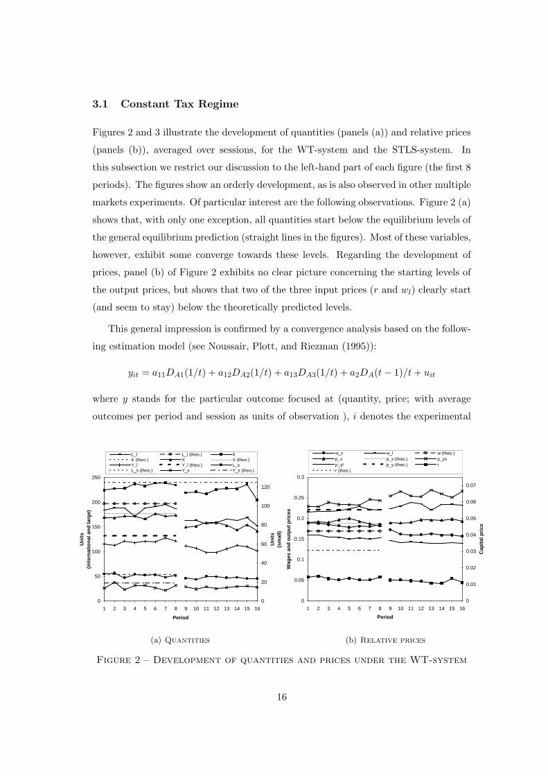
3.1 Constant Tax Regime

Figures 2 and 3 illustrate the development of quantities (panels (a)) and relative prices

(panels (b)), averaged over sessions, for the WT-system and the STLS-system. In

this subsection we restrict our discussion to the left-hand part of each figure (the first 8

periods). The figures show an orderly development, as is also observed in other multiple

markets experiments. Of particular interest are the following observations. Figure 2 (a)

shows that, with only one exception, all quantities start below the equilibrium levels of

the general equilibrium prediction (straight lines in the figures). Most of these variables,

however, exhibit some converge towards these levels. Regarding the development of

prices, panel (b) of Figure 2 exhibits no clear picture concerning the starting levels of

the output prices, but shows that two of the three input prices (r and wl) clearly start

(and seem to stay) below the theoretically predicted levels.

This general impression is confirmed by a convergence analysis based on the follow-

ing estimation model (see Noussair, Plott, and Riezman (1995)):

yit = a11DA1(1/t) + a12DA2(1/t) + a13DA3(1/t) + a2DA(t − 1)/t + uit

where y stands for the particular outcome focused at (quantity, price; with average

outcomes per period and session as units of observation ), i denotes the experimental

0

50

100

150

200

250

1 2 3 4 5 6 7 8 9 10 11 12 13 14 15 16

Period

Un

its

(in

tern

atio

nal

an

d la

rge)

0

20

40

60

80

100

120

Un

its

(sm

all)

L_l L_l (theo.) KK (theo.) X X (theo.)Y_l Y_l (theo.) L_sL_s (theo.) Y_s Y_s (theo.)

(a) Quantities

0

0.05

0.1

0.15

0.2

0.25

0.3

1 2 3 4 5 6 7 8 9 10 11 12 13 14 15 16

Period

Wag

es a

nd

ou

tpu

t p

rice

s

0

0.01

0.02

0.03

0.04

0.05

0.06

0.07C

apit

al p

rice

w_s w_l w (theo.)p_x p_x (theo.) p_ysp_yl p_y (theo.) rr (theo.)

(b) Relative prices

Figure 2 – Development of quantities and prices under the WT-system

16

0

50

100

150

200

250

1 2 3 4 5 6 7 8 9 10 11 12 13 14 15 16

Period

Un

its

(in

tern

atio

nal

an

d la

rge)

0

20

40

60

80

100

120

Un

its

(sm

all)

L_l K K (theo.)X Y_l L_sY_s

(a) Quantities

0

0.05

0.1

0.15

0.2

0.25

0.3

1 2 3 4 5 6 7 8 9 10 11 12 13 14 15 16

Period

Wag

es a

nd

ou

tpu

t p

rice

s

0

0.01

0.02

0.03

0.04

0.05

0.06

0.07

Cap

ital

pri

ce

w_s w_l p_x p_ys p_yl r

(b) Relative prices

Figure 3 – Development of quantities and prices under the STLS-system

session, t the trading period in the session, DAi a dummy variable for session i of the

WT-system which is equal to 1 for i and 0 otherwise, and u the error term. Note that

the coefficients a1i indicate session specific starting values and a2 the asymptotic value

of y in the WT-system (DA = 1 when the WT-system is effective). Strong convergence

is said to hold if the estimated asymptotic value (a2) is not significantly different from

the theoretically predicted level. We will speak of weak convergence if the majority of

the starting values (a1i) are further apart from the theoretical level than the estimated

asymptotic value.

The regression results are presented in Table 4. They show that strong convergence

has to be rejected for a majority of the 18 investigated variables. Only the behavior

of employed capital K, employed labor in the small country Ls, and the relative price

pyl satisfy the strong convergence criterion. However, most variables (10 out of 18)

converge in the weak sense. Furthermore, though most asymptotic values are statisti-

cally significantly different from the predicted levels, the differences are mostly small in

economic terms. Given the complexity of the laboratory economy and the fact that the

theoretical general equilibrium model is a very stylized representation of the economy

we find this a quite remarkable result. In line with the visual impression from Figure 2,

we find that the asymptotic value of all aggregate quantity variables is lower than the

respective theoretical level, with the exception of capital employment and the produc-

17

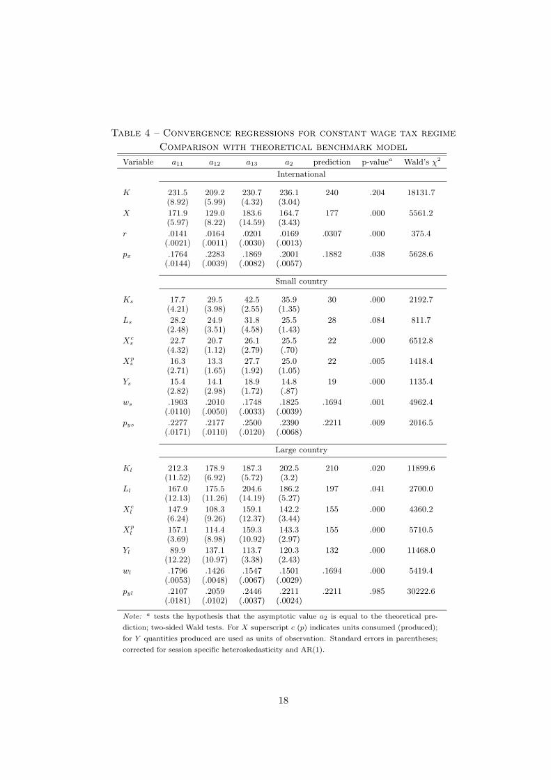
Table 4 – Convergence regressions for constant wage tax regime

Comparison with theoretical benchmark model

Variable a11 a12 a13 a2 prediction p-valuea Wald’s χ2

International

K 231.5 209.2 230.7 236.1 240 .204 18131.7(8.92) (5.99) (4.32) (3.04)

X 171.9 129.0 183.6 164.7 177 .000 5561.2(5.97) (8.22) (14.59) (3.43)

r .0141 .0164 .0201 .0169 .0307 .000 375.4(.0021) (.0011) (.0030) (.0013)

px .1764 .2283 .1869 .2001 .1882 .038 5628.6(.0144) (.0039) (.0082) (.0057)

Small country

Ks 17.7 29.5 42.5 35.9 30 .000 2192.7(4.21) (3.98) (2.55) (1.35)

Ls 28.2 24.9 31.8 25.5 28 .084 811.7(2.48) (3.51) (4.58) (1.43)

Xcs 22.7 20.7 26.1 25.5 22 .000 6512.8

(4.32) (1.12) (2.79) (.70)

Xps 16.3 13.3 27.7 25.0 22 .005 1418.4

(2.71) (1.65) (1.92) (1.05)

Ys 15.4 14.1 18.9 14.8 19 .000 1135.4(2.82) (2.98) (1.72) (.87)

ws .1903 .2010 .1748 .1825 .1694 .001 4962.4(.0110) (.0050) (.0033) (.0039)

pys .2277 .2177 .2500 .2390 .2211 .009 2016.5(.0171) (.0110) (.0120) (.0068)

Large country

Kl 212.3 178.9 187.3 202.5 210 .020 11899.6(11.52) (6.92) (5.72) (3.2)

Ll 167.0 175.5 204.6 186.2 197 .041 2700.0(12.13) (11.26) (14.19) (5.27)

Xcl 147.9 108.3 159.1 142.2 155 .000 4360.2

(6.24) (9.26) (12.37) (3.44)

Xp

l 157.1 114.4 159.3 143.3 155 .000 5710.5(3.69) (8.98) (10.92) (2.97)

Yl 89.9 137.1 113.7 120.3 132 .000 11468.0(12.22) (10.97) (3.38) (2.43)

wl .1796 .1426 .1547 .1501 .1694 .000 5419.4(.0053) (.0048) (.0067) (.0029)

pyl .2107 .2059 .2446 .2211 .2211 .985 30222.6(.0181) (.0102) (.0037) (.0024)

Note:a tests the hypothesis that the asymptotic value a2 is equal to the theoretical pre-

diction; two-sided Wald tests. For X superscript c (p) indicates units consumed (produced);

for Y quantities produced are used as units of observation. Standard errors in parentheses;

corrected for session specific heteroskedasticity and AR(1).

18

tion and consumption of the capital intensive commodity in the small country. Also

two of the three input price variables are too low, while for two of the three output

price variables the asymptote is higher than the theoretical value. This leads to our

first result.

Result 1 A majority of the variables exhibits weak convergence towards the theoretical

general equilibrium levels. The quantity and input price variables are typically converg-

ing from below, while the output prices are typically converging from above.

We have also run convergence regressions for the economic performance indicators un-

employment rate, real GDP, consumer earnings, net capital export, and labor intensity

in the Y-sector. The results of these regressions corroborate the above findings. In

both countries, all five performance indicators are weakly converging to the theoreti-

cally predicted equilibrium values. In both countries the unemployment rate exhibits

even strong convergence (from above) as does real GDP (from below) in the small coun-

try and the Y-production intensity in the large country. There is, however, a caveat to

this result. As will be demonstrated below, this rather positive result does not come

for free, but is associated with relatively large budget deficits.

We now turn to a comparison of the two tax systems in the constant tax regime.

Comparing Figure 2(a) with Figure 3(a) shows that economic activity starts at a lower

level in the experimental sessions with the STLS-system. This holds for the employment

of both input factors, and is accompanied by lower input prices. In particular, output

of the exposed sector X is affected, while its product price px exhibits a clear upward

thrust. To put this outcome into perspective, one has to recognize that in these periods

the small country is facing substantial sales taxes, with a tax rate of 65% and 75% on

the price of X and Y (see Table 1). Recall that these tax rates are not taken from

a theoretical model but determined such that on impact the producers of X and Y

would have to bear the same tax burden as observed under the WT-system. Thus, the

initial economic circumstances are not particularly favorable for a comparatively good

performance of the alternative tax system.

Our primary research questions concern the small country. Therefore, in the fol-

lowing we mainly, but not exclusively, focus on the economic performance regarding

the small country under the two different tax regimes. Figures 4-6 illustrate the de-

velopment of the unemployment rate, the budget surplus, and real GDP, for both tax

19

0

0.1

0.2

0.3

0.4

0.5

0.6

1 2 3 4 5 6 7 8 9 10 11 12 13 14 15 16

Period

Un

emp

loym

ent

rate

WT-system

STLS-system

(a) Small country

0

0.1

0.2

0.3

0.4

0.5

0.6

0.7

0.8

1 2 3 4 5 6 7 8 9 10 11 12 13 14 15 16

Period

Un

emp

loym

ent

rate

WT-system

STLS-system

(b) Large country

Figure 4 – Development of unemployment rates under the two tax

systems

-0.3

-0.2

-0.1

0

0.1

0.2

0.3

1 2 3 4 5 6 7 8 9 10 11 12 13 14 15 16

Period

Rel

ativ

e su

rplu

s

-0.8

-0.6

-0.4

-0.2

0

0.2

0.4

0.6

0.8

Tax

rat

e

Surplus WT-system Surplus STLS-system

Wage tax WT-system Sales tax on X STLS-system

(a) Small country

-0.6

-0.4

-0.2

0

0.2

0.4

0.6

1 2 3 4 5 6 7 8 9 10 11 12 13 14 15 16Period

Rel

ativ

e su

rplu

s

-1

-0.8

-0.6

-0.4

-0.2

0

0.2

0.4

0.6

0.8

1

Tax

rat

e

Surplus WT-system Surplus STLS-system

Wage tax WT-system Wage tax STLS-system

(b) Large country

Figure 5 – Development of budget surplus and tax rates under the two

tax systems

systems (and both countries). Initially, the unemployment rate in the small country

is at a higher level in case of the STLS-system. However, in spite of the high sales

tax rates, there is a clear tendency for this rate to decline over time (Figure 4). This

stays in clear contrast to the development of the unemployment rate under the WT-

system (and the development in the large country, where a wage tax is applied in both

20

10

12

14

16

18

20

22

24

26

1 2 3 4 5 6 7 8 9 10 11 12 13 14 15 16

Period

Rea

l GD

P

WT-system

STLS-system

(a) Small country

30

50

70

90

110

130

150

1 2 3 4 5 6 7 8 9 10 11 12 13 14 15 16

Period

Rea

l GD

P

WT-system

STLS-system

(b) Large country

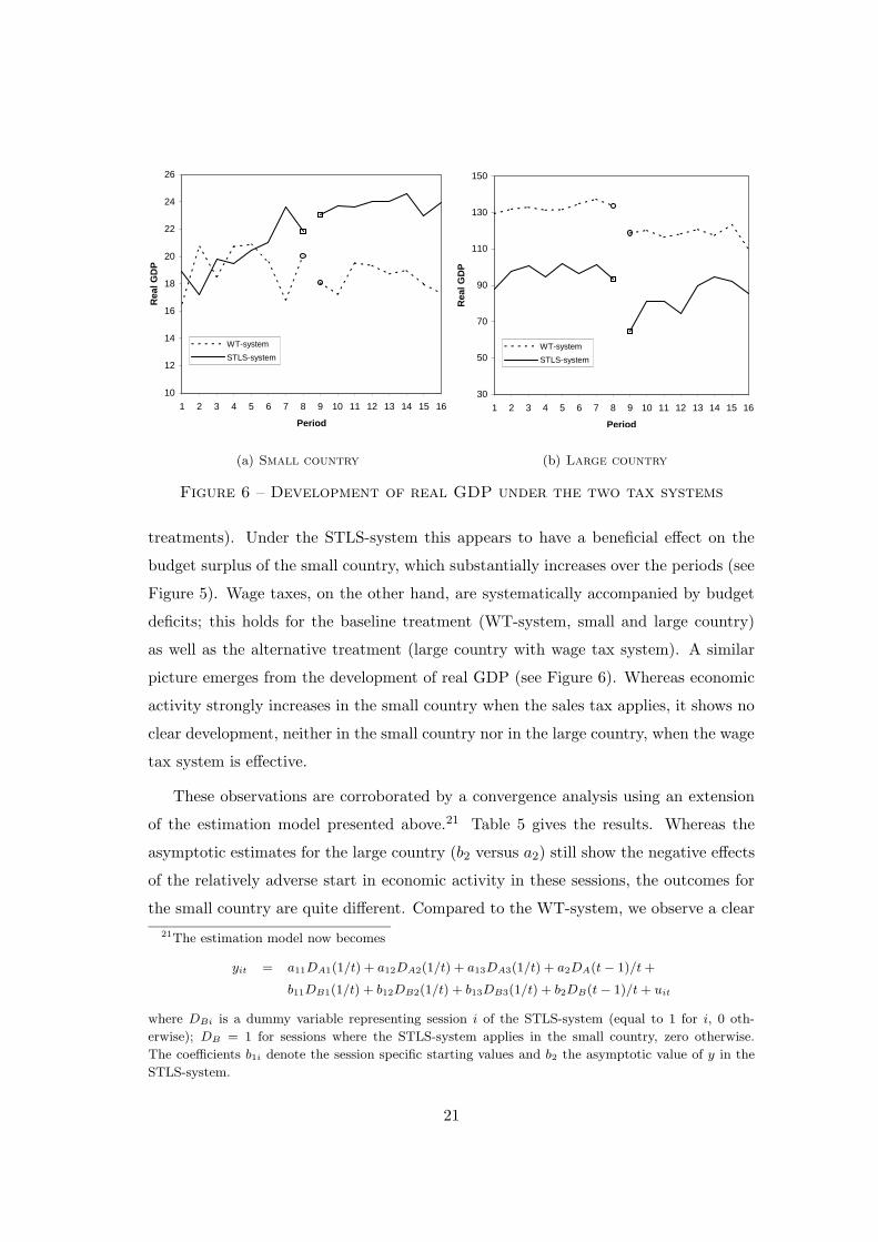
Figure 6 – Development of real GDP under the two tax systems

treatments). Under the STLS-system this appears to have a beneficial effect on the

budget surplus of the small country, which substantially increases over the periods (see

Figure 5). Wage taxes, on the other hand, are systematically accompanied by budget

deficits; this holds for the baseline treatment (WT-system, small and large country)

as well as the alternative treatment (large country with wage tax system). A similar

picture emerges from the development of real GDP (see Figure 6). Whereas economic

activity strongly increases in the small country when the sales tax applies, it shows no

clear development, neither in the small country nor in the large country, when the wage

tax system is effective.

These observations are corroborated by a convergence analysis using an extension

of the estimation model presented above.21 Table 5 gives the results. Whereas the

asymptotic estimates for the large country (b2 versus a2) still show the negative effects

of the relatively adverse start in economic activity in these sessions, the outcomes for

the small country are quite different. Compared to the WT-system, we observe a clear

21The estimation model now becomes

yit = a11DA1(1/t) + a12DA2(1/t) + a13DA3(1/t) + a2DA(t − 1)/t +

b11DB1(1/t) + b12DB2(1/t) + b13DB3(1/t) + b2DB(t − 1)/t + uit

where DBi is a dummy variable representing session i of the STLS-system (equal to 1 for i, 0 oth-

erwise); DB = 1 for sessions where the STLS-system applies in the small country, zero otherwise.

The coefficients b1i denote the session specific starting values and b2 the asymptotic value of y in the

STLS-system.

21

Table 5 – Convergence regressions for constant tax regime

Economic performance indicators compared between the tax systems

Variable a11 a12 a13 b11 b12 b13 a2 b2 p-valuea Wald’s χ2

Small country

Unemploy- .3738 .4479 .2927 .5547 .6151 .2683 .4326 .3134 .001 2667.5ment rate (.0552) (.0779) (.1017) (.0371) (.0357) (.0373) (.0317) (.0135)

Budget −.0927 −.0895 −.0070 .0266 −.0566 .1056 −.1409 .2069 .000 124.3surplus (.0676) (.0804) (.1129) (.0538) (.0923) (.0428) (.0345) (.0251)

Real GDP 13.6 14.1 25.1 15.3 14.2 22.3 20.0 21.8 .039 6392.5(2.02) (1.99) (1.54) (1.44) (1.84) (1.22) (.68) (.56)

Consumer 84.0 88.0 107.1 67.4 18.7 104.6 98.4 87.3 .013 17157.8earnings 1 (7.48) (11.97) (3.60) (6.03) (9.66) (4.78) (2.75) (3.52)

Consumer −13.9 −36.2 172.7 108.4 −25.4 331.5 −59.0 549.7 .000 81.35earnings 2 (80.25) (119.38) (167.24) (147.67) (350.22) (120.64) (48.00) (76.94)

Net capital 8.9 1.3 −16.8 2.8 .4 −.9 −8.1 −9.9 .560 86.5export (6.43) (4.75) (2.85) (4.38) (7.21) (3.42) (2.36) (2.15)

Y-production .5018 .5133 .4011 .5607 .5293 .4975 .3625 .3347 .351 2061.5intensity (.0541) (.0527) (.0438) (.0510) (.0763) (.0522) (.0188) (.0231)

Large country

Unemploy- .4699 .4429 .3506 .6928 .6579 .3653 .4088 .5206 .000 6001.3ment rate (.0385) (.0357) (.0451) (.0257) (.0905) (.0672) (.0167) (.0151)

Budget −.2724 −.1578 −.0425 −.5536 −.6708 −.0388 −.1174 −.2175 .000 1339.8surplus (.0467) (.0154) (.0539) (.0470) (.1587) (.0714) (.0108) (.0258)

Real GDP 120.7 127.2 139.1 71.3 79.5 132.4 134.8 108.6 .000 30313.3(8.16) (2.31) (6.01) (5.25) (18.67) (10.87) (1.64) (3.26)

Consumer 197.3 207.6 214.6 176.9 177.4 197.8 208.9 197.2 .001 136271.6earnings 1 (2.41) (1.93) (2.63) (6.06) (11.93) (5.65) (.95) (3.49)

Consumer −1489.6 −1369.3 −219.5 −3865.3 −3344.2 −379.0 −843.3 −1926.2 .000 1814.1earnings 2 (428.87) (122.11) (492.82) (253.75) (940.85) (665.68) (84.61) (150.48)

Net capital −8.9 −1.3 16.8 −2.8 −.4 .9 8.1 9.9 .560 86.54export (6.43) (4.75) (2.85) (4.38) (7.21) (3.42) (2.36) (2.15)

Y-production .3606 .5322 .4025 .5437 .7096 .6178 .4416 .6612 .000 4060.7intensity (.0257) (.0352) (.0230) (.0493) (.0379) (.0371) (.0157) (.0178)

Note:a tests the hypothesis that the asymptotic values a2 and b2 are equal; two-sided Wald tests. Superscript c (p) indicates units

consumed (produced). Standard errors in parentheses; corrected for session specific heteroskedasticity and AR(1). ‘Unemployment rate’

is defined as the amount of unemployed units of labor relative to the total labor force (endowment) in the respective country; ‘Budget

surplus’ denotes the nominal budget surplus relative to nominal GDP (defined as the total nominal value of the produced goods) in the

respective country; the base ‘year’ for calculating ‘Real GDP’ is the first trading period in each session; ‘Consumer earnings 1’ denotes

average earnings of a consumer in points (‘utility’); ‘Consumer earnings 2’ are ‘Consumer earnings 1’ with the per capita budget surplus

added; ‘Net capital export’ is the difference between total capital sold to the other country and total capital bought from the other

country; ‘Y-production intensity’ denotes the total amount of goods produced in the Y-sector relative to the total amount of goods

produced in the respective country.

22

decrease in the unemployment rate and a substantial improvement in the budget bal-

ance. Also real GDP and consumer earnings net of budget surplus show a statistically

significant better outcome under the STLS- than under the WT-system. Whereas for

the former the better performance is economically not large it is dramatically different

for the latter. When not correcting for budget deficits consumer earnings are statisti-

cally significantly larger under the WT-system. Economically, however, the difference

is not large in that case. The remaining two variables are not significantly different for

the two tax systems. There is no shift in production between the sectors (measured

by ‘Y -production intensity’), while net capital export decreases, but not significantly.

These observations lead to our next result.

Result 2 By the end of the constant tax regime, most economic performance indicators

show a significant improvement for the small country under the STLS-system compared

to the WT-system. Only consumer earnings unadjusted for the budget surplus are sig-

nificantly lower under the STLS-system. In the large country, where in both treatments

the wage tax is applied to finance unemployment benefits, no such development is ob-

served.

Note that these outcomes clearly contradict the intuitive hypothesis concerning the

STLS-system presented at the beginning of the previous section. For constant taxes,

the STLS-system does even better than the WT-system. This holds despite the fact

that the exogenously fixed sales tax rates are in the neighborhood of the unfavorable

general equilibrium.

In the following section we present the results of the trading periods where the tax

rates adjusted to the budget surplus in the previous period: the variable tax regime.

This enables us to investigate the robustness of our findings. Especially, we can examine

the economic impact of changes of tax rates in the different tax systems. Additionally,

it also allows us to test for possible convergence of economic activity in the STLS-

system and, hence, to explore whether economic activity coordinates on one of the two

theoretical general equilibria.

3.2 Variable Tax Regime

When the tax rates start to adjust to the budget surplus in the previous trading period

an economic shock occurs. This can be observed from the development of the quantity

23

variables shown in the panels (a) of Figures 2 and 3. From the former it can be seen

that, under the WT-system, all traded quantities in both countries decrease from period

8 to period 9. Under the STLS-system, the quantities traded internationally and in

the large country also decrease, but now the the traded quantities of local goods in the

small country (Ls and Ys) increase when the tax rates begin to adjust (Figure 3 (a)).

In the last constant tax period all economies with wage taxation are confronted with

substantial budget deficits, whereas large surpluses are generated under the sales tax

system in the small country. Therefore, tax rates increase in the former and decrease in

the latter case (see Figure 5). As illustrated by two economic performance indicators in

Figures 4 and 6, in the economies with wage taxation, this triggers a clearly observable

negative economic shock, with increasing unemployment rates and decreasing real GDP.

Because of this shock, the budget balance does not improve in the transition period 9

(see Figure 5). Thereafter, these economies seem to improve somewhat, showing some

convergence towards a balanced budget and a full utilization of capital (see Figure 3).

However, unemployment stays at a high level, which has a negative effect on outputs,

as manifested by the development of real GDP in Figure 6.22

These developments in the economies where the wage tax system applies are in stark

contrast to the economic development in the small country under the alternative tax

system. First of all, the initial decline in the sales tax rates in period 9 produces positive

economic effects. This is witnessed by the development of the economic performance

indicators in Figures 4 and 6. The unemployment rate drops significantly and real

GDP clearly increases. Note, furthermore, the positive effect on the wage rate (ws),

and the negative effect on the price of the labor intensive good Y (pys), in contrast to the

development under wage taxation (see Figures 2 (b) and 3 (b)). This development is due

to the replacement of the wage tax by a labor subsidy. Remarkably, under the STLS-

system the budget immediately balances, and stays that way over the remaining periods,

with only small deviations. As Figures 4 (a) and 6 (a) indicate, the unemployment rate

and real GDP further improve in later periods, and show convergence towards a level

that is substantially different from the level reached under the WT-system.

22Note, furthermore, that the gap between the values of the economic performance indicators in the

large country narrows over the periods with variable tax rates. We will return to this when presenting

the convergence analysis for the variable tax regime.

24

Table 6 – Convergence regressions for variable tax regime

Economic performance indicators compared between the tax systems

Variable a11 a12 a13 b11 b12 b13 a2 b2 p-valueb Wald’s χ2

Small country

Unemploy- .6647 .5279 .2076 .3200 .2726 .2974 .4807 .2417 .000 2818.1ment rate (.0790) (.0155) (.0845) (.0592) (.0270) (.0411) (.0279) (.0151)

Budget −.3990 −.0357 −.0155 .0151 −.0295 .0061 −.0259 .0038 .210 30.1surplus (.0940) (.0349) (.0450) (.0119) (.0261) (.0177) (.0227) (.0067)

Real GDP 15.1 16.1 26.1 21.3 24.1 22.4 18.9 22.8 .000 8526.7(3.43) (.25) (2.46) (1.76) (1.29) (1.11) (.91) (.56)

Consumer 83.4 86.3 70.7 82.3 76.8 104.8 91.8 89.3 .640 5030.7earnings 1 (4.41) (5.00) (10.25) (8.10) (11.90) (10.82) (2.32) (4.83)

Consumer −353.9 49.6 64.7 122.8 −1.1 114.0 64.2 104.6 .230 447.5earnings 2 (108.24) (47.05) (73.52) (22.09) (64.71) (34.69) (30.73) (13.86)

Net capital 2.0 5.0 −22.0 .1 .7 −23.9 −5.9 −20.1 .000 550.9export (7.48) (1.48) (7.16) (6.47) (3.80) (3.05) (1.04) (1.57)

Y-production .3046 .4229 .4113 .4361 .5061 .4846 .4091 .4204 .709 11007.1intensity (.0471) (.0111) (.0296) (.0654) (.0970) (.0586) (.0107) (.0283)

Large country

Unemploy- .6007 .5046 .4126 .6807 .8258 .6193 .5244 .5838 .043 9030.9ment rate (.0174) (.0676) (.0609) (.0706) (.0842) (.0222) (.0203) (.0213)

Budget −.3274 −.0705 −.0126 −.3562 −.7059 −.3281 −.1249 −.1216 .945 283.4surplus (.0435) (.0705) (.0609) (.1140) 4(.1534) (.0470) (.0344) (.0339)

Real GDP 96.3 117.6 133.3 73.5 48.3 85.1 110.5 98.8 .053 5736.4(3.93) (11.53) (12.01) (15.34) (18.14) (4.99) (3.91) (4.61)

Consumer 196.7 202.4 211.1 188.7 169.5 192.4 203.9 197.5 .008 101716.7earnings 1 (2.16) (6.74) (3.35) (3.19) (8.90) (3.88) (1.51) (1.91)

Consumer −2343.8 −550.1 93.3 −2155.2 −4374.2 −1830.1 −750.2 −935.9 .631 222.7earnings 2 (366.52) (579.34) (481.54) (948.01) (1154.18) (323.99) (282.92) (264.15)

Net capital −2.0 −5.0 22.0 −.1 −.7 23.9 5.9 20.1 .000 550.9export (7.48) (1.48) (7.16) (6.47) (3.80) (3.05) (1.04) (1.574)

Y-production .4409 .4735 .4671 .6344 .6051 .5444 .4484 .5411 .002 32879.1intensity (.0122) (.0528) (.0107) (.0409) (.0860) (.0539) (.0071) (.0289)

Note:a tests the hypothesis that the asymptotic values a2 and b2 are equal; two-sided Wald tests. Superscript c (p) indicates units

consumed (produced). Standard errors in parentheses; corrected for session specific heteroskedasticity and AR(1). ‘Unemployment rate’

is defined as the amount of unemployed units of labor relative to the total labor force (endowment) in the respective country; ‘Budget

surplus’ denotes the nominal budget surplus relative to nominal GDP (defined as the total nominal value of the produced goods) in the

respective country; the base ‘year’ for calculating ‘Real GDP’ is the first trading period in each session; ‘Consumer earnings 1’ denotes

average earnings of a consumer in points (‘utility’); ‘Consumer earnings 2’ are ‘Consumer earnings 1’ with the per capita budget surplus

added; ‘Net capital export’ is the difference between total capital sold to the other country and total capital bought from the other country;

‘Y-production intensity’ denotes the total amount of goods produced in the Y-sector relative to the total amount of goods produced in the

respective country.

25

Table 6 presents the results of the convergence analysis comparing the performance

of the two tax systems for the variable tax regime. These estimation results corroborate

the above observations.

Comparing the estimated asymptotic values a2 and b2, for the small country under

the STLS-system, a significant decrease in the unemployment rate and net capital

export together with a significant increase in real GDP show up. For the budget

surplus, the labor intensity of production, and both of the consumer earnings measures,

no statistically significant differences are found. Observe, however, that the amount of

consumer earnings adjusted for the budget surplus shows a considerable improvement,

too. The outcome of no significant difference in the development of the budget surplus

is due to the convergence towards a balanced budget under both tax systems when tax

rates adjust. Notice, however, that the convergence happens from a negative balance

under the WT-system whereas it convergences from a surplus under the STLS-system.

Not surprisingly, for the large country, the outcomes are worse for the STLS-system

sessions, because of the bad start. Note, however, that the asymptotic values a2 and b2,

which are statistically significantly different for unemployment and consumer earnings

uncorrected for the budget surplus, clearly show a movement towards each other. For

both indicators the starting values are much further apart than the asymptotic values.

Furthermore, the differences seem economically not significant. This pattern is in line

with the observation from the figures indicating that the gap between the values of

the economic performance indicators for this country narrows over the periods with

variable tax rates. The budget surplus is clearly negative and virtually the same under

both systems as are the consumer earnings net of the budget surplus. The significant

difference in net capital export mirrors the result for the small country. The following

result summarizes.

Result 3 Under the variable tax regime, the positive view of the STLS-system as ob-

served for constant taxes is corroborated and enhanced. The economic performance of

the country where the STLS-system is applied further improves and shows a substan-

tially lower unemployment rate and net capital export, as well as a higher real GDP,

compared to its performance under the WT-system. With respect to the other economic

indicators - the budget surplus, consumer earnings, and labor intensity of production -

there are no significant differences in performance.

26

An important further issue concerns the economic effect of changes in the different

tax rates under the two tax systems. Table 7 shows the results of a regression analysis

with respect to the economic performance indicators: unemployment rate, capital em-

ployment, real GDP, consumer earnings, net capital flight, and Y -production intensity.

In addition to the tax rates the number of the trading period is also included as an

explanatory variable, to control for a time trend.

Several observations are in order. First of all, the signs of all tax effects are com-

pletely in line with economic intuition. For both the wage tax and the sales tax it

appears that tax hikes have a negative impact on economic activity and consumer

earnings of the country directly involved. Higher taxes also encourage capital flight.

Furthermore, changes of tax rates in the small country have no spill-over effects on the

large country (the only exception being the effect of a wage tax change on capital flight,

which is due to definition of this variable). An increase of the wage tax in the large

country, however, has a statistically significantly negative effect on consumer earnings

in the small country. The only obscure result concerns the effect of the sales tax on

labor intensity of production.

The regression results clearly show that a wage tax increase has strong adverse

effects on the economic performance in the respective country. This is witnessed by

the statistically and economically highly significant coefficients of the wage taxes τws

in the small country and τwl in the large country, in most regressions. Increasing the

wage tax rate in a country substantially increases unemployment and capital flight and

decreases real GDP and capital employment.

An increase of the sales tax rate in the small country also adversely affects unem-

ployment and real GDP in a statistically significant way. What is striking, though, is

that the magnitude of these effects is substantially smaller than the effects of a wage

tax rate increase. For unemployment the coefficient is .4420 for the the wage tax but

only .1831 for the sales tax. Similarly, real GDP decreases by only 6.85 when the sales

tax increases whereas the marginal decrease of this measure amounts to 11.95 for the

wage tax. For capital employment, consumer earnings, net capital flight, and labor

intensity of production, a change in the sales tax is not even significantly different from

zero. The next result summarizes the most important findings.

27

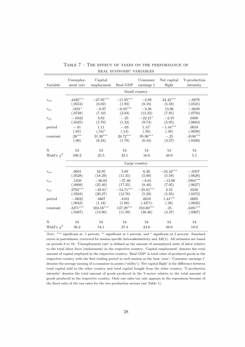
Table 7 – The effect of taxes on the performance of

real economic variables

Unemploy- Capital Consumer Net capital Y-production

Variable ment rate employment Real GDP earnings 1 flight intensity

Small country

τws .4420∗∗∗−27.95∗∗∗

−11.95∗∗∗−2.89 24.42∗∗∗

−.0879(.0554) (6.02) (1.92) (8.18) (5.58) (.0521)

τxs .1831∗−8.87 −6.85∗∗∗

−3.38 13.96 −.0639(.0728) (7.10) (2.03) (13.22) (7.95) (.0750)

τwl −.0342 3.82 −.25 −22.21∗−2.55 .0308

(.0425) (5.70) (1.32) (9.74) (5.95) (.0604)

period −.01 1.11 −.03 1.15∗−1.44∗∗∗ .0018

(.05) (.54)∗ (.14) (.56) (.38) (.0038)

constant .26∗∗∗ 31.30∗∗∗ 26.72∗∗∗ 95.90∗∗∗−.25 .4136∗∗∗

(.06) (6.24) (1.78) (6.44) (4.37) (.0430)

N 54 54 54 54 54 54

Wald’s χ2 106.2 25.5 42.1 16.6 48.0 5.1

Large country

τws .0041 32.95 5.69 6.30 −24.42∗∗∗−.0357

(.0528) (18.29) (11.31) (5.00) (5.58) (.0628)

τxs .1450 −26.03 −27.46 −8.61 −13.96 .1964∗∗∗

(.0808) (25.40) (17.35) (8.40) (7.95) (.0627)

τwl .2793∗∗∗−49.81∗

−54.71∗∗∗−25.61∗∗∗ 2.55 .0238

(.0583) (20.27) (12.76) (5.39) (5.95) (.0472)

period −.0032 .4667 .4183 .6010 1.44∗∗∗ .0005(.0043) (1.18) (1.00) (.4271) (.38) (.0032)

constant .3371∗∗∗ 203.58∗∗∗ 147.29∗∗∗ 210.60∗∗∗ .25 .4485∗∗∗

(.0487) (13.06) (11.39) (38.46) (4.37) (.0367)

N 54 54 54 54 54 54

Wald’s χ2 38.2 54.1 27.4 24.6 48.0 19.0

Note: ∗∗∗ significant at .1 percent, ∗∗ significant at 1 percent, and ∗ significant at 5 percent. Standard

errors in parentheses; corrected for session specific heteroskedasticity and AR(1). All estimates are based

on periods 8 to 16. ‘Unemployment rate’ is defined as the amount of unemployed units of labor relative

to the total labor force (endowment) in the respective country; ‘Capital employment’ denotes the total

amount of capital employed in the respective country; ‘Real GDP’ is total value of produced goods in the

respective country with the first trading period in each session as the base ‘year’; ‘Consumer earnings 1’

denotes the average earning of a consumer in points (‘utility’); ‘Net capital flight’ is the difference between

total capital sold to the other country and total capital bought from the other country; ‘Y-production

intensity’ denotes the total amount of goods produced in the Y-sector relative to the total amount of

goods produced in the respective country. Only one sales tax rate appears in the regressions because of

the fixed ratio of the tax rates for the two production sectors (see Table 1).

28

Result 4 In the small country, compared to the wage tax, an increase in the sales tax

appears to have a much smaller adverse economic impact. The detrimental effect of a

rise in the sales tax on the employment of labor and real GDP is only about half the

effect of an increase in the wage tax. Moreover, whereas there is a significantly negative

effect of an increase in the wage tax on capital, no such effect is found for the sales tax.

All in all, compared to the WT-system, the performance of the STLS-system turns out

to be remarkably good.

What remains to be discussed is whether under the STLS-system economic activities

tend to coordinate on one of the two theoretical general equilibria presented in Table 2.

To this end we performed a convergence analysis for the periods 9 to 16 and compared

the outcomes with the theoretical predictions. Table 8 presents the results. In the

table, column “equil. 1” shows the predictions of the ‘favorable’ general equilibrium

and the column labeled “equil. 2” those of the ‘unfavorable’ one. For the international

variables, which are mainly influenced by the large country, it holds that too little

capital is employed and (accordingly) too little X produced. Both variables, however,

exhibit weak convergence towards the equilibrium values which are virtually identical

in the two general equilibria. On the other hand, the price of capital is too low and the

price of commodity X appears to be too high. All this suggests that the equilibration

process did not yet settle down on the international markets. A similar picture can

be observed for the development of variables in the large country. There, capital and

labor employment as well as the production and consumption of X weakly converge

towards the equilibrium values from below. Concerning the local prices of labor and Y

it can be observed that the former is too low and the latter to high compared to any

of the equilibrium predictions. The budget surplus is weakly balancing from below but

the tax rate τwl is much too high and far removed from any equilibrium value.

We turn now to the most interesting case, the small country in which the alternative

STLS-system applies. Here the results are remarkably different. Three of the five real

variables converge at least weakly to the favorable equilibrium (Ls, Xcs , and Ys). Capital

K and the production level of the capital intensive commodity, Xps , do not converge

but do better than predicted in the favorable equilibrium. The budget balance strongly

converges to zero, while the sales taxes (weakly) converge to the tax rates predicted

by the favorable general equilibrium. Also the wage rate converges from below to the

value predicted in the favorable equilibrium. Only the price of the local good Y does

29

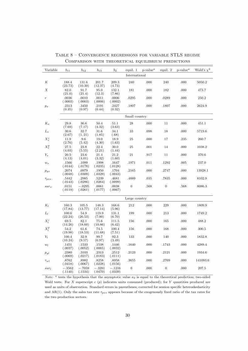
Table 8 – Convergence regressions for variable STLS regime

Comparison with theoretical equilibrium predictions

Variable b11 b12 b13 b2 equil. 1 p-valuea equil. 2 p-valuea Wald’s χ2

International

K 188.4 131.6 201.7 209.3 240 .000 240 .000 5050.2(23.73) (10.39) (12.37) (4.73)

X 82.0 91.7 95.0 132.1 181 .000 182 .000 473.7(21.0) (21.4) (12.3) (7.86)

r .0036 .0010 .0011 .0006 .0295 .000 .0289 .000 250.2(.0003) (.0003) (.0006) (.0002)

px .2313 .3450 .2191 .2427 .1807 .000 .1807 .000 2624.9(0.35) (0.97) (0.44) (0.32)

Small country

Ks 29.8 36.6 50.4 51.1 28 .000 11 .000 451.1(7.69) (7.17) (4.32) (3.63)

Ls 30.6 32.7 31.6 34.1 33 .098 18 .000 5719.6(2.67) (1, 21) (1.85) (.68)

Xcs 11.9 9.6 19.0 18.9 25 .000 17 .235 260.7

(2.76) (5.42) (4.30) (1.63)

Xps 27.5 23.8 22.4 30.0 25 .001 14 .000 1038.2

(4.03) (5.55) (2.21) (1.44)

Ys 20.5 23.6 21.4 21.2 21 .917 11 .000 370.6(4.13) (4.01) (3.32) (1.60)

ws .1566 .1099 .1998 .1647 .1971 .011 .1292 .005 237.0(.0144) (.0178) (.0235) (.0128)

pys .2074 .0979 .1950 .1704 .2165 .000 .2747 .000 13928.1(.0048) (.0309) (.0329) (.0043)

τpxs .5442 .2985 .5239 .4681 .4889 .035 .7835 .000 8102.9(.0143) (.0286) (.0264) (.0099)

surs .0151 −.0295 .0061 .0038 0 .568 0 .568 8086.3(.0119) (.0261) (.0177) (.0067)

Large country

Kl 160.3 105.5 148.3 168.6 212 .000 229 .000 1809.9(17.84) (13.77) (17.14) (5.96)

Ll 100.6 54.9 119.9 131.1 199 .000 213 .000 1749.2(22.24) (26.53) (7.00) (6.70)

Xcl

69.5 82.1 75.6 111.5 156 .000 165 .000 488.2(14.26) (18.60) (10.86) (6.42)

Xpl

54.2 61.6 74.5 100.4 156 .000 168 .000 300.5(19.98) (18.53) (11.68) (7.51)

Yl 100.4 32.9 99.7 92.3 133 .000 140 .000 1832.8(10.24) (9.57) (6.97) (3.49)

wl .1451 .1533 .1538 .1446 .1640 .000 .1743 .000 4289.4(.0037) (.0052) (.0065) (.0032)

pyl .2380 .3103 .2313 .2512 .2123 .000 .2121 .000 1934.6(.0069) (.0217) (.0183) (.0111)

τwl .8762 .8982 .8258 .8958 .3655 .000 .2769 .000 141093.6(.0418) (.0067) (.0228) (.0156)

surl −.3562 −.7059 −.3281 −.1216 0 .000 0 .000 207.5(.1140) (.1534) (.0470) (.0339)

Note:a tests the hypothesis that the asymptotic value a2 is equal to the theoretical prediction; two-sided

Wald tests. For X superscript c (p) indicates units consumed (produced); for Y quantities produced are

used as units of observation. Standard errors in parentheses; corrected for session specific heteroskedasticity

and AR(1). Only the sales tax rate τpxs appears because of the exogenously fixed ratio of the tax rates for

the two production sectors.

30

not show a clear pattern in the small country. The following result summarizes the

main observations.

Result 5 Under the variable tax regime, when the STLS-system obtains in the small

country and the WT-system obtains in the large country, the international real variables

and the real variables related to the large country mostly weakly converge towards to the

equilibrium predictions, from below. The input prices turn out to be too low and the

output prices too high compared to both theoretical equilibria. In contrast, in the small

country the real variables are either converging towards the favorable equilibrium or do

even better than this equilibrium predicts. The wage rate also converges towards the

prediction of the favorable equilibrium. Only the output price for the labor intensive

commodity Y stays too low compared to any of the equilibrium predictions.

Hence, the alternative STLS-system performs better than the WT-system by coordi-

nating economic activity in the direction of the favorable general equilibrium or does

even better than that. In the next section we offer a tentative explanation for this

finding, using theoretical arguments and some further evidence.

4 A behavioral explanation and empirical support

Our experimental results clearly suggest that financing unemployment benefits via sales

taxes, in combination with a subsidy for employment, leads to much better economic

outcomes than using a wage tax, even in a relatively small open economy. Though

disadvantaged at the beginning, due to high tax rates stemming from persistent budget

deficits under the wage tax system and the requirement of equivalent tax burdens

on impact, the STLS-system manifests its beneficial effects immediately. Its better

performance regarding the economic indicators is even further improved when tax rates

start to adjust to the budget balance. Also, it appears that changes in sales taxes have

a much weaker negative economic effect than changes in wage taxes.

Compared to the theoretical predictions of the standard general equilibrium model

the wage tax system has a tendency to do worse. For the STLS-system the theoretical

prediction is ambiguous in the sense that two stable equilibria exist. It turns out that

under this alternative system economic behavior exhibits a tendency to coordinate

on the ‘favorable’ equilibrium or to perform even better than the theoretical model

predicts. In the following we offer theoretical arguments and empirical support for the

following claim, which can explain these observations.

31

Claim 1 Uncertainty about product prices makes producers reluctant to incur produc-

tion costs. This can explain the good economic performance of the sales-tax-cum-labor-

subsidy system in comparison with the wage tax system. Instead of being confronted

with a tax burden up-front on the input of labor, producers under the former system

receive a labor subsidy and only have to pay taxes in proportion to their sales revenues,

which effectively means risk sharing by the government.

To substantiate this claim we offer four pieces of evidence. First, recall from Result 1

that under the constant wage tax regime quantity and input price variables typically

converge from below, whereas output prices seem to converge from above towards the

competitive equilibrium levels of the theoretical general equilibrium model. Although

this theoretical model does not capture all details of our complex lab economy, the

result is suggestive of some downward pressure on the demand for inputs. Also, because

these outcomes are accompanied by a budget deficit. A second piece of evidence in this

respect is obtained by comparing the (after tax) marginal revenue product of labor and

capital with the respective net (i.e. after tax or subsidy) input price. Table 9 shows the

number of cases in which producers’ marginal revenue product exceeds the input price,

using average current prices.23 Assuming random errors, profit maximization would be

consistent with a fraction of 50%. The observed fractions are remarkably different from

this benchmark, however. Our next result summarizes the evidence.

Result 6 Averaging over periods and tax systems, for about 70 percent of the cases

producers’ marginal revenue product of capital (74%) and labor (65%) exceeds the input

price. Taken over all periods, with only one exception in each system, the excess is

always significant. Moreover, comparing the second half of the trading periods with the

first half, there is no systematic decrease in the excess.

This result provides further support for the view that, under both tax systems, produc-

ers are reluctant to buy inputs.24 Interestingly, Noussair, Plott, and Riezman (1995)

observe a similar phenomenon in an experiment concerning international trade.25 These

23Similar results are obtained when the average product price of the previous period is used.24In particular, because we have no evidence of a shortage of capital or labor. On the contrary,

comparing actual labor supply with theoretical labor supply - using the benchmark model and actual

prices - we find excess supply for a fraction of consumers that is significantly larger than 50% (on

average, 94% for the WT-system and 73% for the STLS-system). Concerning capital, the relatively

low capital price also points into the direction of an excess supply (see Figures 2 and 3).25Noussair, Plott, and Riezman (1995) use simultaneous (double auction) input and output markets.

Thus, our results do not seem to be due to the use of sequential markets. Hey and di Cagno (1998),

investigating experimentally two sequential double auction markets, also observe a shortage of trade,

compared to the competitive equilibrium predictions (see also Goeree and Holt 1999).

32

Table 9 – Fraction of cases where producers’marginal revenue product exceeds net input price

WT-system STLS-system

Labor Capital Labor Capital

Small country

1 to 8 0.4583 0.6250 0.6250 0.9583

(0.7646) (0.0557) (0.0557) (0.0000)

X-sector 9 to 16 0.5000 0.6667 0.8750 0.9583

(0.5573) (0.0147) (0.0000) (0.0000)

all 0.4792 0.6458 0.7500 0.9583

(0.6950) (0.0028) (0.0000) (0.0000)

1 to 8 0.5694 0.6944 0.4722 0.6528

(0.1444) (0.0007) (0.7220) (0.0064)

Y-sector 9 to 16 0.5833 0.8472 0.9167 0.6944

(0.0973) (0.0000) (0.0000) (0.0007)

all 0.5764 0.7708 0.6944 0.6736

(0.0399) (0.0000) (0.0000) (0.0000)

Large country

1 to 8 0.6042 0.8333 0.9583 0.9583

(0.0967) (0.0000) (0.0000) (0.0000)

X-sector 9 to 16 0.6250 0.7708 0.7708 1.0000

(0.0557) (0.0001) (0.0001) (0.0000)

all 0.6146 0.8021 0.8646 0.9792

(0.0158) (0.0000) (0.0000) (0.0000)

1 to 8 0.6250 0.6528 0.7361 0.5694

(0.0222) (0.0064) (0.0000) (0.1444)

Y-sector 9 to 16 0.6111 0.5972 0.5556 0.6944

(0.0382) (0.0625) (0.2048) (0.0007)

all 0.6181 0.6250 0.6458 0.6319

(0.0029) (0.0017) (0.0003) (0.6319)

Note: Based on average current period input and output prices and all

periods; within parentheses the probability of obtaining values as least

as extreme as observed when p = 0.5; binomial test, one-sided; n = 48

for periods 1 to 8 and 9 to 16, n = 96 for all periods.

authors conjecture that producers may require a compensation for the market risk they

run, since they may not be able to sell outputs. A likely underlying reason for this

behavior is some form of aversion towards risk or losses. Indeed, theoretical partial

equilibrium models exist indicating that product price uncertainty reduces the factor

demand of risk-averse competitive firms (see the literature mentioned in the Introduc-

33

Table 10 – Correlation of factor employment and

output price uncertainty

St.dev. output price St.dev. output price

WT-system STLS-system WT-system STLS-system

Lys -0.0868 -0.3490 Kys -0.0056 -0.3390(0.5709) (0.0188) (0.9711) (0.0227)

Lyl -0.3198 -0.4796 Kyl -0.3251 0.2455(0.0322) (0.0009) (0.0293) (0.1041)

Lxs -0.3195 -0.5016 Kxs -0.3004 -0.6194(0.0324) (0.0004) (0.0450) (0.0000)

Lxl -0.2721 -0.6669 Kxl 0.0737 -0.5833(0.0706) (0.0000) (0.6304) (0.0000)

Lx -0.2828 -0.6565 Kx -0.0523 -0.6567(0.0598) (0.0000) (0.7331) (0.0000)

Note: Entries show Spearman’s ρ between employment of the mentioned factor in

period t and the standard deviation of the relevant nominal output price in period

t − 1; p-values in parentheses, two-sided tests.

tion), and risk-averse behavior of firms appears to be a realistic assumption.26 Yet,

empirical microeconomic studies of the consequences of market uncertainty for factor

demand are scarce (see Ghosal (1995)).27 Important exceptions are Leahy and Whited

(1996) and Guiso and Parigi (1999). Both of these studies find that investment is

negatively affected by uncertainty.

Taking the standard deviation of transaction prices in the previous period as mea-

sure of expected price uncertainty in the current period, we examine the correlation of

this measure with the employment of capital and labor. Table 10 presents the outcomes.

In line with our conjecture and as suggested by field studies, a mostly significantly neg-

ative correlation shows up. The next result summarizes this third piece of evidence for

our claim.

Result 7 The demand for capital and labor is mostly significantly negatively correlated

with output price uncertainty.

What causes risk averse behavior is not completely clear yet. Recent studies on the

economic significance of emotions suggest that anxiety may play a role, because of the

26According to Stiglitz (1999, p. 254): “There is by now a large body of literature arguing that

normally firms act in a risk averse manner (...)”. Zhang (1998, p. 1753) notes: “Investors of all types

generally exhibit aversion to risk”. For an empirical study showing risk-aversion by firms, see Gunjal

and Legault (1995).27The situation is different for studies focusing on the impact of macroeconomic uncertainty, as

captured by inflation, for instance. These studies typically show a negative effect on private investment

(see Aizenman and Marion 1993, Brunetti and Weder 1998).

34

time lag between inputs and outputs (cf. the motto of our paper). For example, Caplin

and Leahy (2001) argue that by ignoring anxiety conventional measures of risk aversion

underestimate the effects of uncertainty on asset prices. The reason is that because

anxiety is aversive it requires compensation by a higher rate of return. Consequently, an

anxious decision maker may appear more risk averse.28 Another relevant finding in this

context is that the possibility rather than the probability of a negative outcome appears

to be important (Loewenstein, Hsee, Weber, and Welch (2001)), which manifests itself

in overreaction to small probability events (see Harless and Camerer 1994). In the

context of sequential markets it is also interesting that people also seem to treat delayed

outcomes as being uncertain (see Keren and Roelofsma (1995)). These results do not

only provide additional support for our result of a negative effect of price uncertainty

on factor demand, they also indicate that little perceived uncertainty may already

have substantial effects. Thus, it need not be surprising if we do not observe rapid

convergence to competitive equilibrium levels in complex market environments. To

improve theoretical predictions it seems important to take the so far neglected dynamic

behavioral aspects of such market economies into account. A research direction which

is strongly advocated by Akerlof (2002).

Importantly, the overall output price uncertainty turns out to be similar under both

tax systems. In fact, our measure of uncertainty shows some tendency to be larger under

the STLS-system. Together with the above result and the relatively good performance

of the economy under this system this corroborates the view that producers perceive the

uncertainty differently under the WT- and the STLS-system. The fact that under the

latter system the risk can be shared with the government seems to play an important

role here.

For our fourth and final piece of evidence for our claim we return to Table 7. This

table shows that increases in the sales tax have much weaker adverse economic effects

than increases in the wage tax. This finding fits the view that producers are relatively

more concerned with incurring certain costs up-front than with some uncertain costs,

that can be shared with the government, in the future.

All in all, the theoretical arguments and the empirical support for our claim seem

substantial. The evidence presented makes it quite intuitive why the sales tax system

28Experimental evidence of a negative impact of anxiety on risk taking is presented in Bosman and

van Winden (2002).

35

performs so much better than the wage tax system. It also provides a rationale for why

under the STLS-system economic activity is attracted by the favorable equilibrium or

does even better than that. With any aversion to risk or losses, having the government

sharing in the sales revenue risk, instead of having to bear a tax burden up-front,

certainly seems to be the more producer and employment friendly scheme. The more

so when a labor subsidy is included.

5 Conclusion

In this paper we present an experimental comparison of a wage tax system and an

alternative sales-tax-cum-labor-subsidy system as a means of financing unemployment

benefits. Our experimental results are strongly in favor of the alternative system. Un-

der the alternative system, economic activity is directed towards the theoretical equi-

librium without capital flight and with the better economic performance. In particular,

employment and GDP do not decline but sharply increase. Instead of capital flight,

even capital import is observed and the balance of the budget does not deteriorate but

strongly improves.

In our view, producers’ reluctance to incur production costs up-front when facing

product price uncertainty plays a crucial role. We present four pieces of experimental

evidence in support of this claim. First, a convergence analysis using the results of the

theoretical benchmark model appears to be suggestive of a downward pressure on the

demand for inputs. Quantity and input price variables typically converge from below,

and output price variables from above the theoretically predicted levels. Second, for

most producers the estimated marginal revenue product of capital and labor persistently

exceeds the respective input price. Third, the demand for capital and labor turns out

to be mostly negatively correlated with the variance of output transaction prices in

the previous trading period. Finally, we find that increases in sales tax rates have

much weaker adverse economic effects than increases in wage tax rates. This evidence

makes it understandable that the alternative tax system performs much better than

the wage tax system. Instead of having to pay an input tax up-front, producers receive

a labor subsidy while they only have to pay taxes in proportion to whatever the sales

revenues turn out to be. The latter effectively means risk sharing by the government.

36

Furthermore, our claim finds support from some theoretical partial equilibrium models

showing that risk-averse firms indeed employ fewer inputs.

Although, as yet, relatively few macroeconomic experiments have been carried out,

we think that the experience that is now accumulating is of interest from a scientific

as well as policy perspective. For example, our experimental findings are in agreement

with Akerlof’s view that macroeconomics should be behavioral, in the spirit of Keynes

(see Akerlof (2002, p. 428)). An aversion on the side of producers to input taxation

relative to output taxation, due to the elapse of time, is a behavioral factor that seems

to have been neglected in theory. In fact, this finding may have a wider bearing on

the theoretical modeling of how economic agents behave in complex dynamic market

environments. As noted by Plott (2001): “as it turns out, the classical theories of price

adjustment are incomplete” (p. 3), and “experiments teach us about theory and it is

theory that we use when addressing complex and new problems. The progress builds

in slow and in unexpected ways” (p. 27).

37

References

Aizenman, J., and N. P. Marion (1993): “Macroeconomic uncertainty and private

investment,” Economics Letters, 41, 207-210.

Akerlof, G. A. (2002): “Behavioral Macroeconomics and Macroeconomic Behavior,”

American Economic Review, 92, 3, 411-433.

Basu, S. and J. G. Fernald (1997): “Returns to scale in U.S. production: estimates

and implications,” Journal of Political Economy, 105, 2, 249-283.

Batra, R. N., and A. Ullah (1974): “Competitive firm and the theory of input

demand under price uncertainty,” Journal of Political Economy, 82, 3, 537-548.

Blanchard, O., and L. F. Katz (1997): “What We Know and Do Not Know About

the Natural Rate of Unemployment,” Journal of Economic Perspectives, 11, 1,

51-72.

Bosman, R., and F. van Winden (2002): “Global risk, effort, and emotions in an

investment experiment,” CREED working paper, University of Amsterdam.

Bovenberg, A. L. (1994): “Perspectives on tax policy in small and open economies,”

Scandinavian Journal of Economics, 96, 3, 283-287.

Braulke, M., and G. Corneo (2003): “Capital taxation may survive in open

economies,” CESifo Working Paper No.975. University of Munich.

Brunetti, A., and B. Weder (1998): “Investment and institutional uncertainty: a

comparative study of different uncertainty measures,” Weltwirtschaftliches Archiv,

134, 3, 513-533.

Caplin, A., and J. Leahy (2001): Psychological expected utility theory and antici-

patory feelings,” Quarterly Journal of Economics, CXVI, 55-81.

Davis, D. D., and C. A. Holt (1993): Experimental Economics, Princeton University

Press: Princeton.

de Mooij, R.A., and A.L. Bovenberg (1998): “Environmental taxes, international

capital mobility and inefficient tax systems: Tax burden vs. tax shifting,” Inter-

national Tax and Public Finance, 5, 7-39.

38

Diamond P.A., and J.A. Mirrlees (1971): “Optimal taxation and public production

I: Production efficiency, and II: Tax rules,” American Economic Review, 61, 8-27

and 261-278.

Dierker, E. (1972): “Two remarks on the number of equilibria of an economy,” Econo-

metrica, 40, 951-953.

Eaton, J. and H. S. Rosen (1980): “Labor supply, uncertainty, and efficient taxa-

tion,” Journal of Public Economics, 14, 365-374.

Ghosal, V. (1995): “Input Choices under Price Uncertainty,” Economic Inquiry, 33,

1, 142-158.

Goeree, J. K., and C. A. Holt (1999): “Employment and prices in a simple macroe-

conomy,” Southern Economic Journal, 65, 3, 637-647.

Gordon R. H. (1992): “Can capital income taxes survive in open economies?” The

Journal of Finance, XLVII, 3, 1159-1180.

Guiso, L., and G. Parigi (1999): “Investment and demand uncertainty,” Quarterly

Journal of Economics, CXIV, 185-227.

Gunjal, K., and B. Legault (1995): “Risk Preferences of Dairy and Hog Producers

in Quebec,” Canadian Journal of Agricultural-Economics, 43, 1, 23-35.

Harless, D. W., and C. Camerer (1994): “The predictive utility of generalized

expected utility theories,” Econometrica, 62, 1251-1289.

Hartman, R. (1975): “Competitive firm and the theory of input demand under price

uncertainty: comment,” Journal of Political Economy, 83, 6, 1289-1290.

Hartman, R. (1976): “Factor demand with output price uncertainty,” American Eco-

nomic Review, 66, 4, 675-81.

Hey, J. D. and D. di Cagno (1998): “Sequential markets: an experimental investiga-

tion of Clower’s dual-decision hypothesis,” Experimental Economics, 1, 1, 63-85.

Holthausen, D. M. (1976): “Input choices and uncertain demand,” American Eco-

nomic Review, 66, 1, 94-103.

39

Huck, S., K. A. Konrad, W. Muller, and H. T. Norman, H. (2001): “Mergers

and the perception of market power: An experimental study,” SSRN working

paper series.

Kahneman, D., and A. Tversky (1979): “Prospect Theory: An Analysis of Decision

under Risk ,” Econometrica, 47, 2, 263-291.

Keren, G. and P. Roelofsma (1995): “Immediacy and certainty in intertemporal

choice,” Organizational Behavior and Human Decision Processes, 63, 287-297.

Keynes, J. M. (1970): The General Theory of Employment, Interest and Money.

MacMillan: London.

Koskela, E., and R. Schob (2002): “Why governments should tax mobile capital in

the presence of unemployment,” Contributions to Economic Analysis and Policy,

1, 1, Article 1.

Layard, R., S. Nickell, and R. Jackman (1991): Unemployment: Macroeconomic

Performance and the Labour Market. Oxford University Press: Oxford.

Leahy, J.V., and T.M.. Whited (1996): “The effect of uncertainty on investment:

some stylized facts,” Journal of Money, Credit, and Banking, 28, 1, 64-82.

Lian, P. and C. R. Plott (1998): “General equilibrium, markets, macroeconomics

and money in a laboratory experimental environment,” Economic Theory, 12, 21-

75.

Loewenstein, G. F., C. K. Hsee, E. U. Weber, and N. Welch (2001): “Risk as

feelings,” Psychological Bulletin, 127, 267-286.

Noussair, C. N., C. R. Plott, and R. G. Riezman (1995): “An experimental

investigation of the patterns of international trade,” American Economic Review,

85, 462-491.

Noussair, C. N., C. R. Plott, and R. G. Riezman (1997): “The principles of

exchange rate determination in an international finance experiment,” Journal of

Political Economy, 105, 4, 822-861.

40

Plott, C. (2001): “Equilibrium, equilibration, information and multiple markets: from

basic science to institutional design,” California Institute of Technology, mimeo.

Plott, C. R., and P. Gray (1990): “The multiple unit double auction,” Journal of

Economic Behavior and Organization, 13, 245-258.

Quirmbach, H. C., C. W. Swenson, and C. C. Vines (1996): “An experimental

examination of general equilibrium tax incidence,” Journal of Public Economics,

61, 337-358.

Razin, A., and E. Sadka (1991): “International tax competition and gains from tax

harmonization,” Economics Letters, 37, 69-76.

Richter W. F., and K. Schneider (2001): “Taxing mobile capital with labor market

imperfections,” International Tax and Public Finance, 8, 245-262.

Rogerson, R. (1997). ‘Theory Ahead of Language in the Economics of Unemployment’,

Journal of Economic Perspectives, vol. 11, pp. 73-92.

Roth, A. E. (2002): “The economist as engineer: game theory, experimentation, and

computation as tools for design economics,” Econometrica, 70, 4, 1341-1378.

Sandmo, A. (1971), “On the theory of the competitive firm under price uncertainty,”

The American Economic Review, 61, 65-73.

Snower, D. J. (2000): “Evolution of the Welfare State,” Schriften des Vereins fur

Socialpolitik, 271, 35-52.

Sørenson, P. B. (1997): “Public Finance Solutions to the European unemployment

problem?,” Economic Policy: A European Forum, 25, 221-251.

Stiglitz, J. E. (1999): “Taxation, Public Policy, and Dynamics of Unemployment ”,

International Tax and Public Finance, 6, 3, 239-262.

van Winden, F. A. A. M., A. Riedl, J. Wit, and F. van Dijk (1999): “Exper-

imenteel Onderzoek naar het Plan Van Elswijk,” CREED, University of Amster-

dam.

Zhang, G. (1998): “Ownership concentration, risk aversion, and the effect of financial

structure on investment decisions,” European Economic Review, 42, 1751-1778.

41