inplane microwave plasma - comsol.com

Solved with COMSOL Multiphysics 4.0a. © COPYRIGHT 2010 COMSOL AB.

I N P L A N E M I C R O W A V E P L A S M A | 1

I n p l a n e M i c r owa v e P l a sma

Introduction

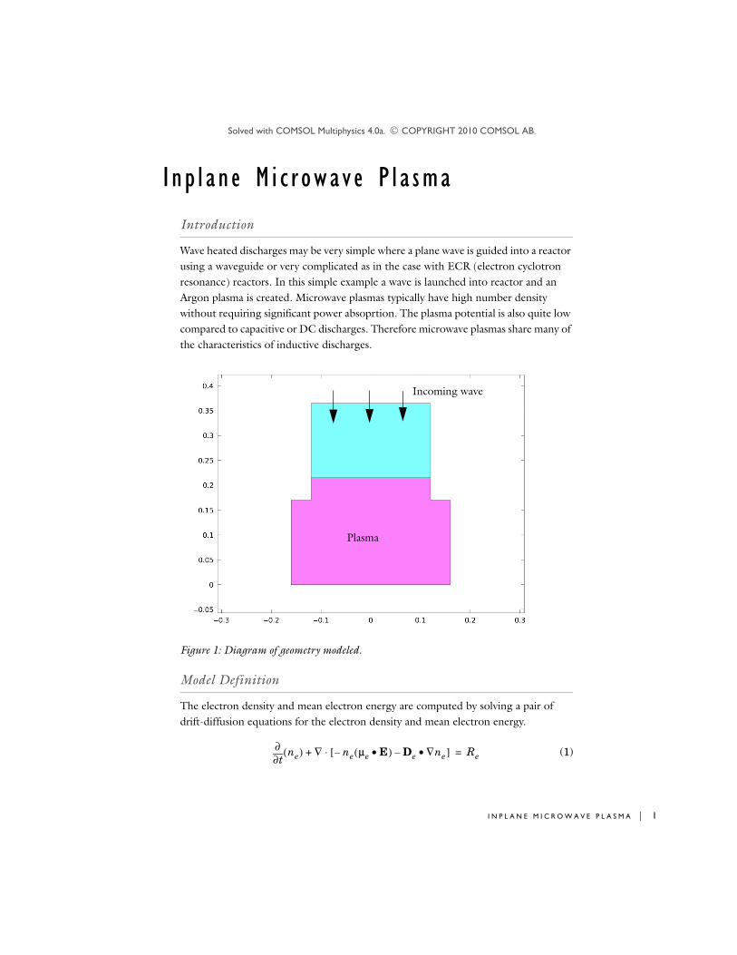
Wave heated discharges may be very simple where a plane wave is guided into a reactor using a waveguide or very complicated as in the case with ECR (electron cyclotron resonance) reactors. In this simple example a wave is launched into reactor and an Argon plasma is created. Microwave plasmas typically have high number density without requiring significant power absoprtion. The plasma potential is also quite low compared to capacitive or DC discharges. Therefore microwave plasmas share many of the characteristics of inductive discharges.

Figure 1: Diagram of geometry modeled.

Model Definition

The electron density and mean electron energy are computed by solving a pair of drift-diffusion equations for the electron density and mean electron energy.

(1)

Plasma

Incoming wave

t∂∂ ne( ) ∇ ne μe E•( )– De ∇ne•–[ ]⋅+ Re=


2 | I N P L A N E M I C R O W A V E P L A S M A

(2)

The electron source Re and the energy loss due to inelastic collisions Rε are defined later. The electron diffusivity, energy mobility and energy diffusivity are computed from the electron mobility using:

. (3)

The source coefficients in the above equations are determined by the plasma chemistry and are written using either rate or Townsend coefficients. Suppose that there are M reactions which contribute to the growth or decay of electron density and P inelastic electron-neutral collisions. In general P >> M. In the case of rate coefficients, the electron source term is given by

(4)

where xj is the mole fraction of the target species for reaction j, kj is the rate coefficient for reaction j (m3/s) and Nn is the total neutral number density (1/m3). The electron energy loss is obtained by summing the collisional energy loss over all reactions:

(5)

where Δεj is the energy loss from reaction j (V). The rate coefficients are be computed from cross section data by the following integral:

(6)

where γ = (2q/me)1/2 (C1/2/kg1/2), me is the electron mass (kg), ε is energy (V), σk

is the collision cross section (m2) and f is the electron energy distribution function. In this example the EEDF is assumed to be Maxwellian.

For non-electron species, the following equation is solved for the mass fraction of each species:

. (7)

t∂∂ nε( ) ∇ nε με E•( )– Dε ∇nε•–[ ] E Γe⋅+⋅+ Rε=

De μeTe= με, 53--- μe= Dε, μεTe=

Re xjkjNnnej 1=

M

=

Rε xjkjNnneΔεjj 1=

P

=

kk γ εσk ε( )f ε( ) εd0

∞

=

ρt∂

∂ wk( ) ρ u ∇⋅( )wk+ ∇ jk⋅ Rk+=



The electrostatic field is computed using the following equation:

. (8)

The space charge density, ρ is automatically computed based on the plasma chemistry specified in the model using the formula:

. (9)

In a microwave reactor the high frequency electric field is computed in the frequency domain using the following equation:

(10)

The relationship between the plasma current density and the electric field becomes more complicated in the presence of a DC magnetic field. The following equation defines this relationship:

(11)

where σ is the plasma conductivity tensor which is a function of the electron density, collision frequency and magnetic flux density. Using the definitions:

(12)

where q is the electron charge, me is the electron mass, ne is the collision frequency and ω is the angular frequency of the electromagnetic field. In this example the inverse of the plasma conductivity is diagonal since there is no external DC magnetic field:

. (13)

∇– ε0εr V∇⋅ ρ=

ρ q Zknkk 1=

N

ne–

=

μr1– E∇×( )∇× k0

2 εrjσ

ωε0---------–

E– 0=

σ 1– J• E=

α qme νe jω+( )------------------------------- β, neqα= =

σ 1–

1β--- 0 0

0 1β--- 0

0 0 1β---

=



P L A S M A C H E M I S T R Y

hemical mechanism consisting of only 3 species and 7 reactions:

Stepwise ionization (reaction 5) can play an important role in sustaining low pressure argon discharges. Excited argon atoms are consumed via superelastic collisions with electrons, quenching with neutral argon atoms, ionization or Penning ionization where two metastable argon atoms react to form a neutral argon atom, an argon ion and an electron. Reaction number 7 is responsible for heating of the gas. The 11.5eV of energy which was consumed in creating the electronically excited Argon atom is returns to the gas as thermal energy when the excited metastable quenches. In addition to volumetric reactions, the following surface reactions are implemented:

When a metastable argon atom makes contact with the wall, it will revert to the ground state argon atom with some probability (the sticking coefficient).

E L E C T R I C A L E X C I T A T I O N

The plasma is sustained through absorption of electromagnetic waves. The Port boundary condition is used to excite the plasma. A total power of 500 Watts is fed into the port and a certain amount of this power is absorbed and a certain amount is reflected. The amount of power absorbed depends on the plasma conductivity which is a function of the electron density and collision frequency.

TABLE 1: TABLE OF COLLISIONS AND REACTIONS MODELED

REACTION FORMULA TYPE

1 e+Ar=>e+Ar Elastic 0

2 e+Ar=>e+Ars Excitation 11.5

3 e+Ars=>e+Ar Superelastic -11.5

4 e+Ar=>2e+Ar+ Ionization 15.8

5 e+Ars=>2e+Ar+ Ionization 4.24

6 Ars+Ars=>e+Ar+Ar+ Penning ionization -

7 Ars+Ar=>Ar+Ar Metastable quenching -

TABLE 2: TABLE OF SURFACE REACTIONS

REACTION FORMULA STICKING COEFFICIENT

1 Ars=>Ar 1

2 Ar+=>Ar 1

Δε(eV)



Results and Discussion

The electron density peaks in the center of the reactor.

Figure 2: Plot of the electron density.



Figure 3: Plot of the electron temperature in the reactor.



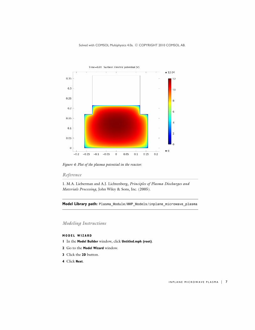
Figure 4: Plot of the plasma potential in the reactor.

Reference

1. M.A. Lieberman and A.J. Lichtenberg, Principles of Plasma Discharges and Materials Processing, John Wiley & Sons, Inc. (2005).

Model Library path: Plasma_Module/MWP_Models/inplane_microwave_plasma

Modeling Instructions

M O D E L W I Z A R D

1 In the Model Builder window, click Untitled.mph (root).

2 Go to the Model Wizard window.

3 Click the 2D button.

4 Click Next.



5 In the Add Physics tree, select Plasma>Microwave Plasma (mwp).

6 Click Next.

7 In the Studies tree, select Preset Studies>Frequency-Transient.

8 Click Finish.

G E O M E T R Y 1

Rectangle 1 (r1)1 In the Model Builder window, right-click Model 1 (mod1)>Geometry 1 and select

Rectangle.

2 Go to the Settings window for Rectangle.

3 Locate the Size section. In the Width edit field, type 0.32.

4 In the Height edit field, type 0.17.

5 Locate the Position section. In the x edit field, type -0.16.

Rectangle 2 (r2)1 In the Model Builder window, right-click Geometry 1 and select Rectangle.





6 In the y edit field, type 0.17.

Union 1 (uni1)1 In the Model Builder window, right-click Geometry 1 and select Boolean

Operations>Union.

2 Select the objects r1 and r2 only.

3 Go to the Settings window for Union.

4 Locate the Union section. Clear the Keep interior boundaries check box.

5 In the Model Builder window, right-click Union 1 (uni1) and select Build All.

6 Click the Zoom Extents button on the Graphics toolbar.

Rectangle 3 (r3)1 Right-click Geometry 1 and select Rectangle.







6 In the y edit field, type 0.215.

7 In the Model Builder window, right-click Rectangle 3 (r3) and select Build All.

8 Click the Zoom Extents button on the Graphics toolbar.

D E F I N I T I O N S

Selection 11 In the Model Builder window, right-click Model 1 (mod1)>Definitions and select

Selection.

2 Go to the Settings window for Selection.

3 Locate the Geometric Scope section. From the Geometric entity level list, select Domain.

4 From the Selection output list, select Adjacent boundaries.

5 Select Domain 1 only.

6 In the Model Builder window, right-click Selection 1 and select Rename.

7 Go to the Rename Selection dialog box and type Walls in the New name edit field.

8 Click OK.

M A T E R I A L S

Material 11 In the Model Builder window, right-click Model 1 (mod1)>Materials and select

Material.

2 In the Model Builder window, right-click Materials and select Material.

Material 11 In the Model Builder window, click Material 1.


3 Go to the Settings window for Material.



4 Locate the Material Contents section. In the Material contents table, enter the following settings:

Material 21 In the Model Builder window, click Material 2.


3 Go to the Settings window for Material.

4 Locate the Material Contents section. In the Material contents table, enter the following settings:

M I C R O W A V E P L A S M A ( M W P )

1 In the Model Builder window, click Model 1 (mod1)>Microwave Plasma (mwp).

2 Go to the Settings window for Microwave Plasma.

3 Locate the Settings section. From the Electric field components solved for list, select Out-of plane vector.

4 Locate the Cross Section Import section. Click the Browse button.

5 In the edit field, type c:sbv4distrmodelsPlasma_ModuleAr_xsecs.txt.

Reaction 11 In the Model Builder window, right-click Microwave Plasma (mwp) and select Heavy

Species Transport>Reaction.

2 Go to the Settings window for Reaction.

3 Locate the Reaction Formula section. In the Formula edit field, type Ars+Ars=>e+Ar+Ar+.

4 Locate the Kinetics Expressions section. In the kf edit field, type 3.734E8.

PROPERTY NAME VALUE

Electric conductivity sigma 0

Relative permittivity epsilonr 1

Relative permeability mur 1

PROPERTY NAME VALUE

Electric conductivity sigma 0

Relative permittivity epsilonr 1

Relative permeability mur 1



Reaction 21 In the Model Builder window, right-click Microwave Plasma (mwp) and select Heavy

Species Transport>Reaction.

2 Go to the Settings window for Reaction.

3 Locate the Reaction Formula section. In the Formula edit field, type Ars+Ar=>Ar+Ar.

4 Locate the Kinetics Expressions section. In the kf edit field, type 1807.

Species: Ar1 In the Model Builder window, click Species: Ar.

2 Go to the Settings window for Species.

3 Locate the Species Formula section. Select the From mass constraint check box.

Species: Ar+1 In the Model Builder window, click .

2 Go to the Settings window for Species.

3 Locate the Species Formula section. Select the Initial value from electroneutrality

constraint check box.

Wave Equation, Electric 11 In the Model Builder window, right-click Microwave Plasma (mwp) and select

Electromagnetic Waves>Wave Equation, Electric.


Plasma Model 11 In the Model Builder window, click Plasma Model 1.

2 Go to the Settings window for Plasma Model.

3 Locate the Model Inputs section. In the T edit field, type 350.

4 In the p edit field, type 101325*(0.1/760).

5 Locate the Electron Density and Energy section. In the μe edit field, type 4E24[1/(m*V*s)]/mwp.Nn.

6 Locate the Conduction Current section. From the σ list, select Electric conductivity

(mwp/wee1).

Initial Values 11 In the Model Builder window, click Initial Values 1.

2 Go to the Settings window for Initial Values.

3 Locate the Initial Values section. In the ne,0 edit field, type 1E17.



Wall 11 In the Model Builder window, right-click Microwave Plasma (mwp) and select Drift

Diffusion>Wall.

2 Go to the Settings window for Wall.

3 Locate the Boundaries section. From the Selection list, select Walls.

Ground 11 In the Model Builder window, right-click Microwave Plasma (mwp) and select

Electrostatics>Ground.

2 Go to the Settings window for Ground.


Surface Reaction 11 In the Model Builder window, right-click Microwave Plasma (mwp) and select Heavy

Species Transport>Surface Reaction.

2 Go to the Settings window for Surface Reaction.

3 Locate the Reaction Formula section. In the Formula edit field, type Ar+=>Ar.



Surface Reaction 21 In the Model Builder window, right-click Microwave Plasma (mwp) and select Heavy

Species Transport>Surface Reaction.


3 Locate the Reaction Formula section. In the Formula edit field, type Ars=>Ar.


Port 11 In the Model Builder window, right-click Microwave Plasma (mwp) and select

Electromagnetic Waves>Port.

2 Select Boundary 7 only.

3 Go to the Settings window for Port.

4 Locate the Port Properties section. From the Wave excitation at this port list, select On.

5 In the Pin edit field, type 500.

6 From the Type of port list, select Rectangular.



M E S H 1

Boundary Layers 11 In the Model Builder window, right-click Model 1 (mod1)>Mesh 1 and select Boundary

Layers.

2 Go to the Settings window for Boundary Layers.

3 Locate the Domains section. From the Geometric entity level list, select Domain.


Boundary Layer Properties1 In the Model Builder window, click Boundary Layer Properties.

2 Go to the Settings window for Boundary Layer Properties.


4 In the Model Builder window, right-click Mesh 1 and select Free Triangular.

Size1 In the Model Builder window, click Size.

2 Go to the Settings window for Size.

3 Locate the Element Size section. From the Predefined list, select Finer.

4 Click the Build All button.

S T U D Y 1

Step 1: Frequency-Transient1 In the Model Builder window, click Step 1: Frequency-Transient.

2 Go to the Settings window for Frequency-Transient.

3 Locate the Study Settings section. In the Times edit field, type 0 .

4 Click the Range button.

5 Go to the Range dialog box.

6 From the Entry method list, select Number of values.

7 In the Start edit field, type -8.

8 In the Stop edit field, type -2.

9 In the Number of values edit field, type 51.

10 From the Function to apply to all values list, select exp10.

11 Click the Add button.

12 Go to the Settings window for Frequency-Transient.



13 Locate the Study Settings section. In the Frequency edit field, type 2.45[GHz].

14 In the Model Builder window, right-click Study 1 and select Compute.

R E S U L T S

2D Plot Group 21 In the Model Builder window, right-click Results and select 2D Plot Group.

2 In the Model Builder window, right-click 2D Plot Group 2 and select Surface.

3 Go to the Settings window for Surface.

4 In the upper-right corner of the Expression section, click Replace Expression.

5 From the menu, choose Microwave Plasma (Drift Diffusion)>Electron temperature

(mwp.Te).

6 In the Model Builder window, right-click Surface 1 and select Plot.

2D Plot Group 31 Right-click Results and select 2D Plot Group.

2 In the Model Builder window, right-click 2D Plot Group 3 and select Surface.

3 Go to the Settings window for Surface.

4 In the upper-right corner of the Expression section, click Replace Expression.

5 From the menu, choose Microwave Plasma (Electrostatics)>Electric potential (V).

6 In the Model Builder window, right-click Surface 1 and select Plot.

inplane microwave plasma - comsol.com

Documents