innovative large-scale energy storage technologies …...d6.3 impact analysis and scenarios design...
TRANSCRIPT

Co-funded by the European Union’s Horizon 2020 research and innovation programme under Grant Agreement no. 691797
Innovative large-scale energy storage
technologies and Power-to-Gas concepts
after optimisation
Impact Analysis and Scenarios design
Due Date 31 May 2018 (M27) Deliverable Number D6.3
WP Number WP6 Responsible Herib Blanco, RUG
Author(s) Cécile Reviewers Helge Föcker (UST), Andrea Mazza (POLITO), Ettore Bompard
(POLITO), Simon Verleger (DVGW), Johannes Ruf (DVGW), Wolfgang Köppel (EBI), Praseeth Prabhakaran (EBI), Frank Graf (DVGW)
Status Started / Draft / Consolidated / Review / Approved / Submitted / Accepted by the EC / Rework
Dissemination level
� PU Public
PP Restricted to other programme participants (including the Commission Services)
RE Restricted to a group specified by the consortium (including the Commission Services)
CO Confidential, only for members of the consortium (including the Commission Services)

D6.3 Impact Analysis and Scenarios design Page 2 of 114
Document history
Version Date Author Description
1 2017-10-03 Herib Blanco Draft 2 2017-11-13 Herib Blanco Additional sections incorporated to ensure a more
complete description of the model and data 3 2018-03-13 Herib Blanco Model review performed by DVGW and ECN.
Model has been modified and results updated 4 2018-04-11 Herib Blanco Comments from DVGW-EBI, UST, POLITO, EIL,
ECN incorporated

D6.3 Impact Analysis and Scenarios design Page 3 of 114
Content
Executive Summary ........................................................................................................................... 7
1 Introduction ................................................................................................................................. 8
1.1 Context and background ................................................................................................. 8
1.2 Approach ........................................................................................................................ 8
1.3 Objectives of the study ................................................................................................... 9
1.4 Intended audience .......................................................................................................... 9
1.5 Interaction with other activities within the project .......................................................... 10
1.6 Document structure ...................................................................................................... 10
2 Literature Review ...................................................................................................................... 11
2.1 Previous studies ........................................................................................................... 11
2.2 Model features and trade-offs ....................................................................................... 16
2.3 Gaps observed in literature and closed in this study ..................................................... 17
3 Model topology and structure .................................................................................................. 18
3.1 Model description ......................................................................................................... 18
3.2 Exogenous input ........................................................................................................... 19
3.3 Technology potentials ................................................................................................... 19
3.4 Gas system .................................................................................................................. 20
3.5 LNG / LMG infrastructure .............................................................................................. 21
3.6 Energy efficiency for space heating in buildings ........................................................... 22
3.7 CO2 network ................................................................................................................. 24
3.8 Hydrogen Network ........................................................................................................ 24
3.9 Sectorial use of hydrogen ............................................................................................. 26
3.10 Electricity Network ........................................................................................................ 27
3.11 Power surplus estimation .............................................................................................. 27
3.12 Other flexibility options (storage and DSM) ................................................................... 28
3.13 Transport fuels ............................................................................................................. 29
3.14 Biomass network and potential ..................................................................................... 30
4 Key policies ............................................................................................................................... 32
4.1 Primary Energy Consumption (PEC) ............................................................................ 32
4.2 Renewable Energy ....................................................................................................... 32
4.3 CO2 constraint .............................................................................................................. 33
4.4 Emission trading system (ETS) ..................................................................................... 33
4.5 Effort sharing decision (non-ETS) ................................................................................. 34

D6.3 Impact Analysis and Scenarios design Page 4 of 114
4.6 Nuclear energy ............................................................................................................. 34
5 Assumptions and data .............................................................................................................. 37
5.1 PtM performance .......................................................................................................... 37
5.2 Hydrogen Network ........................................................................................................ 37
5.3 Sectorial use of hydrogen ............................................................................................. 40
5.4 Other CO2 uses ............................................................................................................ 41
5.5 LMG uses ..................................................................................................................... 42
5.6 Biomass potential ......................................................................................................... 42
6 Scenario definition .................................................................................................................... 44
7 Results ....................................................................................................................................... 46
7.1 Energy, electricity and cost overview for scenarios ....................................................... 46
7.2 Natural gas and PtM gas price comparison .................................................................. 49
7.3 Gas supply and demand ............................................................................................... 51
7.4 Seasonal component of PtM ......................................................................................... 55
7.5 CO2 sources and sinks ................................................................................................. 57
7.6 Drivers and barriers for PtM .......................................................................................... 58
8 Conclusions .............................................................................................................................. 62
9 References ................................................................................................................................ 64
Appendix 1. Macro-economic and techno-economic data and assumptions .............................. 77
Appendix 2. Wind and PV potentials in JRC-EU-TIMES and benchmarking ................................ 83
Appendix 3. Gas trading capacities between countries covered in JRC-EU-TIMES model ........ 85
Appendix 4. Gas transmission and distribution network costs .................................................... 86
Appendix 5. Electricity network representation in JRC-EU-TIMES .............................................. 88
Appendix 6. VRE representation and power surplus estimation in JRC-EU-TIMES .................... 92
Appendix 7. Full list of parameters and scenarios ........................................................................ 95
Appendix 8. Complementary figures and tables for results ....................................................... 103
Appendix 9. CO2 footprint of electricity grid across Main scenarios in comparison to current values ................................................................................................................................ 108
Appendix 10. Price differential between PtM and natural gas for Realistic scenario. ............... 109
Appendix 11. Electricity and hydrogen balance for Cyprus during day and night in Realistic scenario .......................................................................................................................................... 110
Appendix 12. Supply technologies composition for heat demand ............................................. 111
Appendix 13. Fuel mix for different transport modes across main scenarios ........................... 112
Appendix 14. Electricity mix per country and time slice for 95 % CO2 reduction, no CO2 storage and higher PV and wind potentials (“Realistic” scenario) ............................................ 114
Index of Figures

D6.3 Impact Analysis and Scenarios design Page 5 of 114
Figure 1. Methane sources and uses considered in JRC-EU-TIMES. ......................................... 20
Figure 2. Residential sector demand breakdown for energy efficiency calculation. ..................... 23
Figure 3.CO2 sources and uses considered in JRC-EU-TIMES. ................................................. 24
Figure 4. Structure of the hydrogen supply and delivery chain in JRC-EU-TIMES. ..................... 25
Figure 5. Technology coverage of steel industry in JRC-EU-TIMES. .......................................... 26
Figure 6. Technology pathways for fuel production and use for final demand. ............................ 30
Figure 7. Biomass sources (left) and sinks (right) covered in JRC-EU-TIMES. ........................... 31
Figure 8. CO2 trajectory to 2050 for different targets. ................................................................. 33
Figure 9. Development of the capacity of the currently installed nuclear power fleet in the EU. .. 36
Figure 10. Capex contribution to hydrogen production cost for transport pathways. ................... 38
Figure 11. (a) Biomass potential distribution by type of source. (b) Supply cost curve for biomass ................................................................................................................................................... 43
Figure 12. Final energy demand by energy carrier across main scenarios. ................................ 47
Figure 13. Total annual system cost split by sector and marginal CO2 price. .............................. 48
Figure 14. Price comparison between NG and PtM across main scenarios. ............................... 50
Figure 15. Gas supply (lower) and demand (upper) breakdown across main scenarios. ............ 52
Figure 16. Fraction of PtM production stored in each season across all scenarios. .................... 56
Figure 17. CO2 sources and sinks across main scenarios. ......................................................... 57
Figure 18. Main parameters with influence on PtM deployment. Green means it favors PtM, while red means it hinders its deployment. ........................................................................................... 59
Figure 19. Distribution by country for (a) natural gas reserves and installed capacity of (b) LNG, (c) import pipelines and (d) underground storage. ....................................................................... 77
Figure 20. (a) Breakdown of shale gas reserves by production cost and (b) Distribution by country. ....................................................................................................................................... 78
Figure 21. Suitable rooftop area per country and per sector for EU28+ (based on [85]). ............ 83
Figure 22. Comparison of area available for PV between JRC-EU-TIMES and LBST study [87]. 83
Figure 23. Onshore wind potential in JRC-EU-TIMES in comparison to reference studies [85,87]. ................................................................................................................................................... 84
Figure 24. Sources and steps followed to convert gas prices to infrastructure cost. ................... 86
Figure 25. Gas prices for base year for large and small scale consumers. ................................. 87
Figure 26. Annual investment for different sectors based on installed capacity. ......................... 87
Figure 27. Electricity network covering production, delivery and end use included in JRC-EU-TIMES. ........................................................................................................................................ 89
Figure 28. Cumulative distribution for hourly PV production during summer day (blue area) and winter day (red area) time slices (taken from [13]). ...................................................................... 92
Figure 29. VRE representation and surplus estimation in JRC-EU-TIMES. ................................ 93
Figure 30. Storage sizing based on VRE surplus. ...................................................................... 93
Figure 31. Sectorial split of final energy demand in main scenarios. ......................................... 104
Figure 32. Technology contribution to electricity production in main scenarios. ........................ 105
Figure 33. RES and VRE penetration across scenarios. .......................................................... 105
Figure 34. RES and VRE penetration for “Realistic scenario”. .................................................. 105
Figure 35. Electricity demand split by users with no grid (hydrogen), transmission (industry) and distribution. ............................................................................................................................... 106
Figure 36. PtM capacity across EU28+ for all scenarios. .......................................................... 106
Figure 37. Fraction of PtM production stored in each season across all scenarios. .................. 107
Figure 38. CO2 sources for “Alternative” scenario (detail of Figure 17). .................................... 107
Figure 39. Specific CO2 emissions for electricity production across Main scenarios. ................ 108
Figure 40. Change in specific CO2 emissions for electricity generation in EU28. ...................... 108
Figure 41. Price differential between PtM and natural gas for Realistic scenario. ..................... 109
Figure 42. Electricity and hydrogen balance for Cyprus during representative day (left) and night (right). ....................................................................................................................................... 110

D6.3 Impact Analysis and Scenarios design Page 6 of 114
Figure 43. Technology mix to satisfy heat demand in main scenarios. ..................................... 111
Figure 44. Fuel mix for different transport modes across main scenarios (a) Buses (b) Heavy Duty (c) Cars (d) Marine transport ............................................................................................. 113
Figure 45. Normalized electricity mix by (a) Time slice (b) Country. ......................................... 114
Index of Tables Table 1. RES penetration, scope and coverage of PtM studies [20]. ........................................... 12
Table 2. Flexibility options and features included in PtM studies [20]. ......................................... 13
Table 3. Representation of the residential sector and alternatives for insulation. ........................ 22
Table 4. Combination of fuels use by transport sector. ............................................................... 29
Table 5. Base and extreme techno-economic parameters for methanation. ................................ 37
Table 6. Contribution of individual conversion steps to final hydrogen production cost for 2025. 38
Table 7. Base and extreme techno-economic parameters for hydrogen production with PEM. ... 39
Table 8. Techno-economic parameters for hydrogen production with SOEC. ............................. 39
Table 9. Techno-economic parameters for hydrogen use in residential and commercial sectors [156]. ........................................................................................................................................... 40
Table 10. Techno-economic parameters for steel reduction with hydrogen [107]. ....................... 40
Table 11. Techno-economic parameters for Power to Liquid technologies in 2030 [161]. ........... 41
Table 12. Benchmark values for techno-economic parameters of PtL (Fischer-Tropsch route). .. 41
Table 13. Investment and efficiency for heavy-duty transport for 2010 – 2050 [164]. .................. 42
Table 14. Investment and efficiency for buses for 2010 – 2050 [164]. ........................................ 42
Table 11. Annual activity limits for biomass sources in 2050 (in PJ/year) [132]. .......................... 43
Table 16. Key parameters varied across scenarios to identify trends and shifts in the system. ... 45
Table 17. Relative ranking of parameters having influence on PtM deployment. ......................... 60
Table 18. Fuel prices used in JRC-EU-TIMES from POLES and the EU Roadmap 2050 [185]. .. 77
Table 19. Techno-economic parameters for storage technologies in 2050. ................................ 79
Table 20. Dimensions assumed per type of dwelling for insulated surface calculation. ............... 80
Table 21. Thermal coefficient and cost for retrofit measures in residential space heating. .......... 80
Table 22. Input and output streams for direct methanation of biogas [94,191]. ........................... 81
Table 23. Input and output streams for CO2 capture from biogas with amines [94,191]. ............. 81
Table 24. Techno-economic parameters for gas liquefaction. ..................................................... 82
Table 25. Techno-economic parameters used as sensitivities for PtL for target setting. ............. 82
Table 26. Maximum gas trading capacities between regions in JRC-EU-TIMES for 2020 in PJ. . 85
Table 27. Trading matrix for EU28+ with neighboring countries. ................................................. 89
Table 28. Maximum electricity trading capacities between regions in JRC-EU-TIMES for 2025 in GW. ............................................................................................................................................ 91
Table 28. Processes and commodities present for the storage technologies in JRC-EU-TIMES. 94
Table 29. Further parameters varied across scenarios to identify trends in the system (complements Table 16 on page 46). .......................................................................................... 95
Table 30. Rationale for scenario selection. ................................................................................. 96
Table 31. Combination of variables used for scenarios. .............................................................. 99
Table 32. CO2 price for constraint on total CO2 emissions (values represent marginal prices). . 103

D6.3 Impact Analysis and Scenarios design Page 7 of 114
Executive Summary
In the context of this study, Power to Gas (PtM) refers to the production of methane by reaction of hydrogen with captured CO2. PtM is a technology vector providing the link between the power system and others. It can facilitate the integration of variable renewable energy (VRE) and avoid its curtailment. It can make use of CO2 as carbon source. Based on this, this report uses an energy model (to cover all the sectors) with a cost optimization approach to understand the role that PtM plays in alternative future scenarios. The model allows the trade-off with other flexibility options (e.g. DSM1, grid expansion, wind/solar ratio, excess of capacity and other storage technologies) and has all the possible value chains for PtM, where the choice for the optimal pathways is made based on cost. Furthermore, the model has the capacity expansion component which allows obtaining both optimal capacity (for all technologies) and energy generated for different conditions. The model has a European scale and includes all 28 EU member states, Switzerland, Norway and Iceland (EU28+). The main limitations of the model are its temporal (12 time slices per year) and spatial (one node per country) resolution. The various scenarios were evaluated based on parametric variation. 22 parameters that are related to either the system (e.g. CO2 storage) or the technology (e.g. PtM Capex) were varied to create over 120 scenarios, out of which 55 were selected for more detailed analysis. This allows identifying on one hand what the critical parameters to promote PtM deployment are and on the other hand the role (capacity and activity) the technology has in alternative configurations of the energy system. For 21 out of the 55 low carbon scenarios, PtM capacity lies in the range of 40 to 200 GW. Based on the model analysis, PtM arises for scenarios with 95 % CO2 reduction target, no CO2 underground storage and low Capex (75 €/kW only for methanation). Capacity deployed across EU is 40 GW (8% of gas demand) for these conditions, which increases to 122 GW when liquefied natural gas (LNG) is used for marine transport. The simultaneous occurrence of all positive drivers for PtM, which include limited biomass potential, low Power-to-Liquid performance, use of PtM waste heat (to increase efficiency), better electrolyzer performance (400 €/kW and 86% of the input electricity recovered as hydrogen), can increase this capacity to 546 GW (75 % of gas demand). Gas demand is reduced to between 3.8 to 14 EJ (compared to ~20 EJ for 2015) with lower values corresponding to scenarios that are more restricted. Gas is largely displaced by renewable sources in electricity and by electricity (i.e. heat pumps) in space heating. Annual costs for PtM are between 2.5 and 10 bln€/year with EU28’s GDP being 14.8 trillion €/year (2016). Results indicate that direct subsidy of the technology is more effective than taxing the fossil alternative (natural gas) if the objective is to promote the technology. A high VRE is a necessary, but not sufficient condition for PtM. Even countries with up to 95 % electricity from VRE did not have PtM. The system drivers (such as CO2 storage potential, CO2 reduction targets and VRE penetration) have a larger influence than the technology drivers. Results indicate that even with low PtM Capex (< 100 €/kW) and highest efficiency for the technology, the deployment is zero if CO2 storage is still an alternative. Output from this study should be complemented with other models that have a higher temporal and spatial resolution.
1 Demand Side Management

D6.3 Impact Analysis and Scenarios design Page 8 of 114
1 Introduction
1.1 Context and background
The EU has set the target of at least 80% GHG emissions reduction for 2050 (compared to 1990)2. This requires large efforts in all sectors, especially in the power sector, which has to be almost completely decarbonized. Part of the solution is the use of: renewable energy sources (RES), energy efficiency, biomass and CCS (carbon capture and storage). The most important contributors to RES are wind and solar (variable RES or VRE), which are characterized for their high fluctuations and unpredictability. Therefore, the system needs to be ready to accommodate and deal with these perturbations and will require more flexibility to integrate them. Power to Gas (PtG)3 arises as an alternative to deal with the power surplus when the generation from VRE exceeds the demand, complementing other flexibility measures like storage, DSM, electricity grid expansion, excess of installed capacity. Energy can be transformed in another energy carrier that can be used in different sectors. Some of its advantages are: use of existing infrastructure, high energy density, low specific energy cost, seasonal storage and fast response. PtM can play a relevant role as storage and technology vector for a system with high share of RES. However, it needs large improvement in cost and efficiency to be competitive with other comparable technologies. For more detail, refer to other Deliverables of the project (e.g. D8.104, D8.11, due at the end of the project) Storyline and Scenarios document. Nevertheless, the technology does not come without challenges. Currently, it is in the early stages of development (Technology Readiness Level – TRL [1–3] 5-7 [4,5]) and more research is needed to de-risk it and promote its large scale deployment. Economically, it needs a low electricity price (< 10 €/MWh [6,7]), specific Capex (currently up to 1500 €/kW of synthetic gas [6,8]) and high number of operational hours (> 3000 hours to reduce the Capex contribution to the cost) to reach a similar price to the fossil derived natural gas. Environmentally, it needs a low electricity CO2 footprint [9–12] (< 50 gCO2e/kWh) to represent a better alternative than fossil gas and lead to net CO2 reduction (compared to the baseline).
1.2 Approach
This study aims to explore alternative low CO2 emission scenarios (reduction targets of > 80%), where it is envisioned that PtM will play a key role and understand better the drivers for the role of the technology and the circumstances that promote its use in the energy system. The approach chosen is cost optimization of the entire energy system looking at the longer term (2050) and at a large scale (European level). The reasons for this selection are: (1) PtM is a technology acting as technology vector and there lies the importance of looking beyond power; (2) only in the long term low carbon scenarios will be achieved; (3) most of previous studies focus on a local or national scale with few considering the dynamics of the entire EU region; (4) optimal PtM capacity is an output of the model (instead of exogenous). More detail on the model features and reason for selection of this approach are discussed in Section 2.2. Some of the key aspects that can be evaluated with this approach are: RES fraction (or CO2 reduction target) that makes PtM necessary (or result in a lower cost system), amount of PtM use in different scenarios (capacity and energy), difference in deployment due to different technology parameters (cost and efficiency), comparison with competing flexibility options and additional cost
2 https://ec.europa.eu/clima/policies/strategies/2050_en 3 PtG refers to both hydrogen and methane, PtM is used to refer to methane only 4 DX.YY refers to other deliverables within this project, where X is the work package and YY is the consecutive number of the deliverable within that work package

D6.3 Impact Analysis and Scenarios design Page 9 of 114
for presence/absence of the technology. To explore these issues, an energy model will be used, which allows analyzing the evolution of the capacity mix considering both the investment and operational component. The energy model used is JRC-EU-TIMES, owned by the Joint Research Center from the European Commission and which has full documentation available [13]. It has been used in the past for evaluation of low carbon scenarios for the power sector [14], role of electricity storage [15], hydrogen [16], VRE potential with a higher spatial segregation (for Austria) [17] and integration of a DC power flow model [18] and competition between powertrains for a low carbon future transport [19]. It also has multiple reports available5. It is a technology rich (bottom-up) model, which covers the EU-28 plus Switzerland, Norway and Iceland6, where each member state (MS) is one region. Its temporal horizon is from 2010 to 2050 (although it can be used beyond this timeframe). To reduce calculation time, it uses hierarchical clustering into representative hours of a year (24 time slices for the power sector and 12 for others), when there are different levels and compositions of supply and demand. It covers 5 sectors (residential, commercial, industry, transport and agriculture). The model is further described in Section 3. The approach followed is parametric analysis, where individual parameters are changed and their effect is evaluated on both the entire system and the specific technology. Cost optimization is only the first step to identify the best routes to satisfy energy needs, while subsequent steps should include behavioral aspects of consumers, actors with different interests, market representation and selection of competing policies, among others.
1.3 Objectives of the study
There are two main objectives for this study: 1. Quantify the impact methanation has in the energy system. This impact is defined based
on changes in energy balances (competition between commodities), costs (investment needed, but also reflected as commodity prices) and trading (e.g. gas import) for a wide range of methanation capacity deployed across EU. Part of the impact also includes the competition between Power-to-X technologies (hydrogen, methane and liquids) to provide flexibility to the power system and facilitate the integration of VRE.
2. Identify what the drivers and barriers are for methanation and construct potential future scenarios where methanation could play a significant role. This set of scenarios is meant to provide a consistent basis for other partners to analyze different dimensions of the technology deployment.
The impact in this study is limited to the energy system. This is to be complemented with the environmental, legal and social dimensions provided by other deliverables in the project (D5.8, D7.2/D7.3 and D7.8 respectively) to establish the overarching impact of methanation to be estimated using Cost-Benefit Analysis (CBA, D7.6). A secondary objective is to determine what the preferred pathways for methanation are. This includes what the preferential use for the gas is, what the preferred CO2 source is and the use of underground storage for the methane produced.
1.4 Intended audience
This report is intended to develop understanding of the role of the technology in alternative future scenarios for the energy system. Some aspects are outside the scope and the reader is referred to other deliverables within this project in case this is the main information being searched: macroeconomic impact (D8.8), specific NPV analysis from the perspective of an investor (D8.4), specific European and national policy recommendations (D8.11), role considering the economic,
5 https://ec.europa.eu/jrc/en/publications-list/%2522jrc-eu-times%2522 6 Referred from this point onwards as “EU28+”

D6.3 Impact Analysis and Scenarios design Page 10 of 114
social and environmental impact (D7.4 and D7.6), detailed interaction with the power grid (D6.4) and interaction with the gas grid (D5.7).
1.5 Interaction with other activities within the project
Input:
Output:
1.6 Document structure
The report is organized in the following manner: Section 2 gives an overview of the literature review on energy models evaluating PtM and how the current study covers gaps left by those, Section 3 covers the basics of the modeling approach with more detail included as Appendix, Section 4 introduces some of the key policies that have a large effect over the energy system, Section 5 summarizes some of the key assumptions and values, Section 6 presents the scenario definition, Section 7 focuses on the results and trends observed over the related parts of the energy system and Section 8 summarizes the conclusions.
Task Responsible partner
Information Use
5.4 RUG - LCA data for technologies with separate operational component - Indicators to be used
Extend PtM impact beyond energy and economy to include environmental impact. This is to be reported in Deliverable 5.8 and not part of the current report.
7.2 EIL Learning curves for Capex
Capex will depend on research, deployment and learning which T7.2 is looking in more detail. This has a direct impact on total cost and deployment.
Task Responsible partner
Information Use
6.3 POLITO Wind, solar and PtM installed capacities
Analyze electricity grid operation with a higher variable generation and possible flexibility provided by electrolyzers
7.1 ECN Installed capacities, energy balances and costs
Take economic output from Task 6.2 and extend it with externalities and social aspects as part of the CBA (Cost-Benefit Analysis)
7.2 EIL Promising PtG pathways from a systems perspective and PtG contribution in future energy systems
The model is Task 6.2 has all the value chains and optimal ones are chosen based on cost. EIL can use these value chains for more specific optimization (e.g. sizes or specific technologies)
8.2 RUG Electricity price for different renewable penetration, energy mixes and CO2 prices
Prices are endogenous in the model used and can be correlated to changes in the scenarios. T8.2 can use these (internally generated) values instead of taking other scenario studies.

D6.3 Impact Analysis and Scenarios design Page 11 of 114
2 Literature Review
This section is divided in three parts: 1. Looking at all the previous studies, elements covered and main conclusions; 2. General features that can be included in a model and trade-off between completeness, complexity and relation to the model used; 3. Gaps observed in literature and the ones closed with this study
2.1 Previous studies
23 studies were found to fall in the same category as this study and which were used for comparison [20]. The common criteria for this selection were:
• PtM specifically with methane as product (also with H2+CH4 possibility, but not H2 only). • PtM capacity had to be the result of cost optimization (to understand its role in an optimal
mix). • One study [21] has an exogenous defined capacity (exception to rule above), but was
included for the insight of the operational performance of PtM. An hourly resolution model with operational constraints and integer component is used. [22] has a similar approach, but considers only hydrogen (and not methane) and therefore, was not included.
• Covering the entire energy system or at least covering different flexibility options and time aggregation or hourly simulation over a year. Therefore, studies like [23–26] that look either only at levelized cost of electricity in isolation or have limited competition with other flexibility options were not included.
• Language: English. The characterization of the studies is shown in Table 1. Furthermore, since PtG competes with other flexibility options is important to specify what options were considered in the different studies (Table 2) to know if PtM arises because of limited technologies available. 11 of the studies come from the same project (Neo Carbon project), use the same model, with the same approach and assumptions. Therefore, these have been included only once in both Tables (identfiied with “*”).

D6.3 Impact Analysis and Scenarios design Page 12 of 114
Table 1. RES penetration, scope and coverage of PtM studies [20].
RES Management Sectors included Geographical Scale
RES Penetration
/%
Specific cost
/€/kW
Demand size
/TWh
PtM Size
/TWh Power Gas Mobility Regional National Europe Global
Plessmann 2014 [27] 100 940 28600 1690 x - - - - - x
Moeller 2014 [28] 0–100 1880 22 0.184 x - - x - - -
Kotter 2015 [29] 100 900 4.5 0.7 x x - x - - -
Ahern 2015 [21] 38 - 68 0.6 x x - - x - -
Vandewalle 2015 [7] 75 800 218 5.43 x x - - x - -
Clegg 2015 [30] 15–30 - 1150 0.079 x x - - x - -
Jenstch 2014 [31] 85 750 1600 0.01 x x - - x - -
ECN 2013 [32] 10–35 - 620 5.1 x x x - x - -
*LUT 2015 [33–43] 100 614 11481 407.6 x x x - - -
Schaber 2013 [44] 60–85 1100 2030 0–18 x x - - x x -
Henning 2015 [45] 527 1100 1891 0.095 x x x - x - -
Palzer 2014 [46] 70–100 1500 1385 788 x x - - x - -
de Boer 2014 [47] 3–25 - 100
0.001–0.004 x - - - x - -
7 This considers the entire energy system, whereas power sector is covered 100% by RES 8 PtG has a power rating of 87 GW and an annual use of 224 TWh

D6.3 Impact Analysis and Scenarios design Page 13 of 114
Table 2. Flexibility options and features included in PtM studies [20].
Fle
xib
le
gen
era
tio
n
Co
st
learn
ing
cu
rve
En
do
gen
ou
s
ele
ctr
icit
y
pri
ce
Hyd
rog
en
o
nly
CO
2 s
ou
rces
Tra
nsm
issio
n
netw
ork
DS
M
Dem
an
d
ela
sti
cit
y
Op
tim
al
win
d/P
V
Po
wer
to
Heat
Sh
ort
-term
sto
rag
e
Th
erm
al
sto
rag
e
En
erg
y
eff
icie
ncy
Plessmann 2014 [27] - - - - - - - - x - x x -
Moeller 2014 [28] - x - - - x - - x - x - -
Kotter 2015 [29] - x - - x - - - x x x - -
Ahern 2015 [21] - - - - x x - - - - - - -
Vandewalle 2015 [7] - - x - - - - - - - - - -
Clegg 2015 [30] - - x x - x - - - - - - -
Jenstch 2014 [31] x x x - - x x - x x x - -
ECN 2013 [32] x x x x - x x - x - x - -
*LUT 2015 [33–43] x - x - - x - - x x x x -
Schaber 2013 [44] - - x x - x - - x x - - -
Henning 2015 [45] - x - - - - - - x x - x -
Palzer 2014 [46] x - - - - - - - x x x x x
de Boer 2014 [47] - - - - - - - - - - - - -

D6.3 Impact Analysis and Scenarios design Page 14 of 114
14
Comments around the studies are divided in two main categories: (1) non-technical, addressing coverage of the studies and areas that have not been explored (2) technical, aiming to understand better the role, size for PtM and comparison with other integration measures. In terms of sectoral coverage, 9 of the studies do consider more than the power network and take into account that the gas can be used for the heating and industrial sector as part of the gas network. Only 2 include the mobility sector as one possible final use for the product. Nevertheless, in [32] this option only arises when CCS and nuclear are not part of the technology portfolio. However, hydrogen is the end product rather than methane. Most of the studies are on the national level, with 4 of them focusing on Germany. Only one [27] has a global scale, while it has the advantages of considering over 160 countries with a high spatial (1º x 1º latitude x longitude) and temporal (1 year with hourly steps) resolution, splitting the storage in short-term, PtG and thermal and using a 100% RES system9, it has the limitations that it does not consider other sectors or flexibility options, there is no energy exchange between adjacent networks (copper plate between regions, but no connected regions more than 100 km apart) and neglects hydro and biomass potential. With respect to technical conclusions, the main ones are captured below:
• Mobility sector. Some mixed conclusions are obtained. From [45], PtM is an enabling technology that allows achieving RES penetrations higher than 82%. Even though above such percentage, most of the transport (60%) is with electricity and only ~20% with hybrid gas-battery, PtM has to be part of the mix since its absence causes non-feasibility of the scenarios. For the boundary value of 82%, PtM leads to a total system cost reduction of 25% compared to a scenario where the technology is not available. PtM capacity is ~140 GW compared to ~550 GW for wind and solar, where most of it is actually methanation rather than hydrogen. This could also be because both wind and solar reach their maximum potential and to increase their share or having lower footprint a better use of the already produced energy has to be implemented. On the other hand, in [32], sensitivities were done for different specific Capex for the electrolyzer, CO2 reduction target (up to 85%), targets for wind and solar capacity (affecting the variability), fuel prices, technology restrictions (CCS, nuclear and biomass), lower investment cost for H2 transport application and variable H2 content in the natural gas grid. From all these, only when the potential for CCS and biomass is limited or when the limit for the hydrogen content in the gas network is too low, some of the product is absorbed by the transport sector. For this case, not methane, but hydrogen is the final product, while the electrolyzer becomes significant in size (19 GW) with respect to the rest of the system (~30 GW).
• PtM role. The largest contribution is in [27], where it represents one quarter of the total annual energy exchanged by storage and almost 6% of the total annual generated electricity. However, given the limitations mentioned earlier in this section, this only provides an upper value that will become more realistic once flexibility options are considered. In [29], the PtM role is also significant, representing almost 25% of the annual electricity demand (although no mention is made to installed energy capacity10). However, this study deals with covering 100% of the electricity with RES and using the surplus for the heating sector. Hence, Power-to-Heat is used when there is co-occurrence between power surplus and heating demand and the rest being used for PtM. Curtailment is minimal, being only significant when Power-to-Heat is not available. The constant portion of the energy produced by the system is the electricity fraction, with the total varying per
9 Note that this study was not considered in Table 2 because given the limited choices for flexibility, it resulted in 65% of the energy produced not being used immediately, increasing the need for storage to 25% of the demand on annual basis and 6% on a single cycle (installed capacity), which from other studies seem to be a result of the limited number of choices 10 Installed power capacity is 218 MW, compared to an average demand of 328 MW.

D6.3 Impact Analysis and Scenarios design Page 15 of 114
15
scenario depending on the amount absorbed by PtM, Power-to-Heat and curtailed. In [46], PtG energy capacity represents almost 6% of the annual demand with the total energy exchanged in a year about 18%. However, sources of flexibility in generation come from combined cycle using gas from PtM and there is no hydro or biomass that could provide additional flexibility. Additionally, there is no interconnection consideration or DSM which could alleviate the short term fluctuations and avoid the need of the surplus being diversified to gas or heat.
• Seasonality use. In [27], the total storage capacity is equivalent to 30 days of continuous discharge (but only 22 days of daily demand) and has an annual use of 1.2 cycles. Even though the largest component for storage is thermal, the ratio between annual use and capacity (4800 TWh vs. 73.6 TWh) leads to 65 full cycles in a year, which seems to indicate thermal storage is not being used for seasonal fluctuations. This is different from [46], where thermal plays the major role in seasonal storage in combination with CHP operation and has almost three times the PtM capacity. For most of the LUT studies, PtM has < 0.4 cycles a year, being used as seasonal storage when the demand is expanded to the industrial gas and around 1.5-2.2 cycles when only the power sector is considered.
• Cost impact. The absence of PtM in the technology portfolio can lead to an increase in system cost for a high RES penetration. For [29], the cost increased by 10% when PtM was absent. In [30], the focus is on operational costs rather than total (considering investment), but these are reduced by 4-9% depending on the level of penetration (15-30%). In [48], using PtM to satisfy the industrial demand, actually results in an electricity price increase of almost 30%.
• Effect of cost learning curve over PtG role. In [29], a base cost of 900 €/kW is used with the sensitivity being up to 2500 €/kW. Up to 1800 €/kW, there is a marginal change in capacity and full load hours, but it does increase the system cost by ~7%. For 2500 €/kW, PtG role is greatly (by ~60-70%) diminished, being partially replaced by Power-to-Heat and batteries and resulting in a system cost increase of almost 10%.
• Effect on gas grid. In [30], the introduction of PtM with an equivalent capacity of one third of the total installed capacity led to a reduction of 3-8% of the seasonal storage, given that part of the gas demand is covered by PtM. Furthermore, PtM covering part of the gas demand also reduces the seasonal gas price spread by 4-16%11. [7] makes the explicit split between the effects over the electricity and the gas network. For the gas network, there is a marginal effect over gas imports in the long term, with the largest difference being for RES integration rather than PtM. Gas flexibility (defined as additional gas needed due to the use of gas turbines to balance wind fluctuations) is around 12% higher with PtM. In the shorter term, there could be situations where the gas demand is low or even absent and all the gas being consumed has been generated by PtM. For these cases, marginal costs of PtM would be dictating the gas price rather than imported or produced gas. Market should be adjusted to deal with these periods of time.
11 Upper values represent a higher VRE penetration with wind and solar production being almost doubled

D6.3 Impact Analysis and Scenarios design Page 16 of 114
16
2.2 Model features and trade-offs
There are a set of features each model can cover and trade-offs to be done to limit model complexity and calculation time, where no model includes all features. Therefore, it is important to understand which ones are covered in this study, how these complement previous studies and what the remaining gaps are. Key features are:
• Hourly time step. This allows better estimating the electricity surplus and hourly choices on options to manage it. It better captures generation flexibility (ramping of power plants) and storage role.
• Capacity expansion. Some models [21,30,49] focus on the operational component without finding an optimal PtM capacity for a given scenario. Capacity constitutes an exogenous input rather than an output. This could lead to overestimating the role of PtM since the capacity used might not be needed.
• Energy system coverage. Some models [29,30,50,51] focus on the power sector and dealing with power surplus rather than using the surplus for other sectors (e.g. PtX12) or finding alternatives routes to deal with the gas demand. Therefore, the coverage should be the entire energy system instead of power only.
• Grid expansion. The model should be able to make the trade-off between using (or curtailing) power surplus and investing in the grid to find a sink far enough from the source. For this, the model should have both the investment component and at least a simplified grid representation.
• Other flexibility options. With more alternatives to accommodate fluctuations, there is a lower chance of overestimating PtM role. The model should cover as many as possible from: optimal wind/PV ratio (due to its complementary patterns [52–54], DSM, short and long term storage, grid expansion, flexible generation, PtX, to make sure the model has enough outlets for any possible electricity surplus.
• Endogenous commodity prices. PtM economic case is directly dependent on the prices for electricity/hydrogen and methane. These are determined by supply/demand dynamics. Models should capture dynamics that determine these prices rather than take them as exogenous assumptions.
• Geographical scope. PtM has been analyzed on a local [50,55,56], national [57–59], regional [33,36,41] and global [23,51] scale. Resolution, data requirement and conclusions will be different depending on the scale of the model. A higher spatial resolution will require either small geographical scope or fewer model features from this list.
• Technology performance. The study should assess the difference on deployment due to different cost or efficiency since this remains a large uncertainty for the technology due to its needs for development and limited deployment.
• Variable RES/CO2 targets. Need for PtM is greater for low carbon systems [28,45] and it is important to understand how its role can change for a variable target of the system.
Not all of these have been covered by a single study and the challenge lies in trying to cover as many as possible while still using the right tool for the right purpose and still keeping model complexity on a manageable level (both for solving and understanding of results) [20]. Similarly, the current study aims to cover as many features as possible. The investment component and capacity expansion is considered, where the optimal PtM capacity is an output of the model. It covers the entire energy system, as well as flexibility options, where PtM is in direct competition with storage, hydrogen, Power-to-Liquid (PtL), power to heat and DSM, among others. It calculates prices endogenously based on supply and demand curves. It has the option of installing new capacity or introducing new technologies to affect the supply curve and it has the alternative to shift the energy carriers used to satisfy final demand to shift the demand curve. A key feature of the model is that the end use demand is not defined as power, gas, oil demand, but instead the services that are satisfied with those commodities (e.g. number of houses, space to 12 PtX = Power to X = Power to Heat, Hydrogen, Methane, Methanol and other liquids

D6.3 Impact Analysis and Scenarios design Page 17 of 114
17
be heated, materials, traveling distance) and the energy carrier used to satisfy those needs is an endogenous option. Part of the sensitivities done include technology performance parameters and variables CO2 targets to cover gaps observed in previous studies. An area where a trade-off has been made and where further work will be needed is the temporal and spatial scales. The model represents the year in 12 time slices (24 TS for power sector) and additional constraints are introduced to avoid overestimating the role of RES, but its output will differ from an hourly simulation. At the same time, each country is a single node, there is no spatial allocation within the node for generation and consumption and there is a simplified consideration of the transmission and distribution grid.
2.3 Gaps observed in literature and closed in this study
Some of the gaps observed based on this literature review are:
• There is no single model that covers all the flexibility options. There are two studies [31,32] that cover 8 out of the 13 features identified as key for PtM. This study in contrast will cover 12 (excluding flexible generation which includes parameters like ramp-up, minimum stable generation and start-up costs).
• Only two studies cover the transport sector. • There is only one study on a European scale, where most studies cover a national scale
(an exception are the studies by LUT which usually focus on a region, but the one were Europe was included aggregated Europe in 8 regions [36]).
• A systematic variation of scenario parameters to evaluate PtM deployment was only done in [32], which is based on the Dutch energy system.
This study works towards closing the gap of determining PtM capacity on a European scale with an energy wide model that counts with enough flexibility options to deal with power surplus. This is seen as relevant since some studies [50,56,60–62] only look at the possible use of power surplus for PtM without considering if there are better options or even if the alternative will have a positive economic return, while others [63–65] look at the potential and possible outlook for the technology based on cost, performance and foreseen electricity growth without establishing the trade-off with other options for either electricity surplus, CO2 use or satisfying end demand. This study considers the use of LNG for the transport sector in heavy-duty trucks, buses and marine transport. Different from previous studies, hydrogen can be used in sectors other than transport including industry (refineries, ammonia and steel), residential and commercial (µ-CHP). The model also includes PtL that provides a competition for CO2 and hydrogen needed for PtM. It also includes the hydrogen infrastructure cost (pipelines, compression, refueling stations) that would favor the on-site use (for PtM/PtL).

D6.3 Impact Analysis and Scenarios design Page 18 of 114
18
3 Model topology and structure
This section starts with a general description of the model followed by a more detailed look at the sections relevant for PtG. The model has been thoroughly described before [13,15,16,66,67] and this section does not intend to duplicate such documents, but instead to build upon them and in some cases goes in more detail explaining the scope of the model. This section builds upon that effort and explains the scope of the model in more detail. The criteria to reflect information in this section is either (1) Sections that have been improved with respect to those previous publications or (2) Due to its relevance for PtG to make sure it is clear what is included (and how it is represented) in the model. Based on this, areas of the model relevant for PtG are explained below. To simplify the content, explanation is focused on topology and assumptions, while a more specific explanation has been included as Appendix.
3.1 Model description
The modeling approach is based on cost optimization covering the entire energy system and it includes investment, fixed, annual, decommissioning and operational cost as well as taxes, subsidies and salvage value as part of the objective function. Due to the capacity expansion component and scope further than power (commercial, residential, industry and transport), the compromise is in temporal (12 time slices for a year and 24 for the power sector) and spatial (one node per country) resolution. The software used is TIMES (The Integrated MARKAL-EFOM System) [68–70], which is a bottom-up (technologically rich), multi-period tool suitable to determine the system evolution in a long term horizon. The model uses price elasticities of demand to approximate the macroeconomic feedback (change in demand as response to price signals), which allows transforming the cost minimization to maximization of society welfare. Technology representation is achieved through a reference energy system, which provides the links between processes. Each process is represented by its efficiency (input-output), cost and lifetime. Prices are endogenously calculated through supply and demand curves. Several policies can be added including CO2 tax [71], technology subsidy [72][73], regulations, targets, energy efficiency [74], feed-in tariffs, emission trading systems [75] and energy security [76], among others. A common application involves the exploration of decarbonization pathways [77–80]. Some of the key output parameters of the model are the capacity needed for each technology, energy balances for each country in each time period, trading, emissions and total costs. Key assumptions of the approach include: perfect foresight (all the prices, demand for services and balances are known from the beginning of the period), perfect competition (there are no individual players that can influence prices), central optimization (lowest cost decisions made regardless of sectors or borders), no market consideration and rational behavior of players. This particular model has around 22 million parameters, 850000 values for activity level (production for a specific process) considering the type of process, period, time slice, region and vintage, while there are almost 1.7 million of values for energy balance (commodity flows) for each scenario. Calculation time can be 1 to 2 hours depending on number of milestone years. Some of the aspects that are not covered with JRC-EU-TIMES are: macro-economy (except for the interaction through elasticity), power plant operation (e.g. minimum stable generation, start-up time and costs), land use, climate (e.g. reduced form geophysical model), behavioral choices for private transport, supply of resources (e.g. biomass), agriculture and non-CO2 emissions and pollutants. Natural cycles (hydrological, carbon, water) in the biosphere, political and social aspects are also omitted in the approach. Due to the focus on energy systems (leaving changes in agricultural practices, biomass burning, decay, petrochemical, solvents out of the scope) and only CO2 (no CH4, N2O, NOx and pollutants), the model effectively covers around close to 80% of

D6.3 Impact Analysis and Scenarios design Page 19 of 114
19
GHG emissions, noting that for 2014, the energy sector represented 68% of the GHG emissions, industry 7% and agriculture 11%, while CO2 was 90% of the GHG emissions [81].
3.2 Exogenous input
The key input parameters to the model are:
• Macroeconomic data. This includes services and material demand projections, differentiated by economic sector and end use service. These are taken from [82], which uses the GEM-E3 model. The other macroeconomic variables are the fuel prices for oil, gas and coal, which are in line with [82] and taken from POLES. Global fuel prices reach almost 100$/bbl for oil, 10 $/MMBtu (7.9 €/GJ) for gas and 100$/ton for coal. See Appendix 1 for more details on evolution and commodities.
• Base year calibration. Mainly done with Eurostat and an internal JRC database13. For more detail on the categories used for each sector, refer to [13].
• Technology parameters. This covers cost, efficiency and lifetime for the various technologies beyond the base year. For electricity, these are mostly taken from an internal database at JRC and for the other sectors mostly from [83]. Technology specific discount rates are from [82], which were generated with PRIMES.
• Technology potentials. The present and future sources (potentials and costs) of primary energy and their constraints for each country are from the GREEN-X model and the POLES model, as well as from the RES2020 EU funded project, as updated in the REALISEGRID project.
• Interconnection between countries. This is relevant for electricity (ENTSO-E and Annex 16.9 of [13] for specific values), CO2 transport costs (taken from [84]) and gas.
A further variable affecting PtM is indigenous gas reserves, since it can affect gas supply and ultimately gas price, which in turn directly affects PtM profitability since it is the main product. 60% of the reserves are held by Norway and with total gas reserves for EU28+ of 610 EJ at an average production cost of 1.2 €/GJ. Shale gas could add 545 EJ of reserves, although at a higher production cost of 15.4 €/GJ. For the rest of the values on LNG, pipeline and storage capacities considered in the model refer to Appendix 1.
3.3 Technology potentials
PV and wind potentials are important given that they will affect the electricity price and the higher they are, the higher the need for flexibility. For PV, an initial assumption of 10 m2 per capita is made, which already includes suitable roof area, green and brownfields, combined with an average irradiation of 850 W/m2. This could lead to up to 1600 GW of PV capacity for the region, compared to ~100 GW deployed by 201614. This is still a conservative value, where using data from [85], an average of 33 m2 per capita for EU28+ (see Appendix 2) was obtained. Because of this, scenarios with a higher potential equivalent to 25 m2 per capita are evaluated as part of the sensitivities. Similarly, for wind, JRC-EU-TIMES uses a conservative estimate of 320 GW of onshore capacity (to put it in perspective, installed capacity in 2015 was 140 GW [86]) and 730 GW for offshore (only 11.1 GW in 2015 [86]). Other estimates are actually between 1020 and 1460 GW [87] respectively and even 1740 GW only for onshore [85]. Therefore, the approach has been to use the conservative estimate as reference point to avoid an overreliance on this technology and use higher estimates as sensitivities to quantify the impact. See Appendix 2 for more information on VRE potentials. Biomass potential is relevant since it can satisfy end services where PtM could play a role and because it can act as CO2 source for PtM. This potential ranges widely in literature [88] and this study considers between 10 and 25.5 EJ/year (Appendix 1 for categories and breakdown). This parameter is more relevant when considering the competition with transport and Power-to-Liquid, which is part of an upcoming publication (in 13 JRC Integrated Database on the European Energy Sector (IDEES) 14 https://www.eea.europa.eu/publications/renewable-energy-in-europe-2017/download

D6.3 Impact Analysis and Scenarios design Page 20 of 114
20
preparation). A limitation on CO2 underground storage is not considered, since it has been shown [89] that potential is orders of magnitude higher than needed. Global potential is almost 11000 GtCO2 when considering saline aquifers, whereas IEA estimates foresee 120-160 GtCO2 of storage will be needed by 2050. The limitation assessed is the social acceptance aspect (rather than potential), where the extreme case is used (no CO2 storage allowed). For geothermal potential, there are two contrasting sources. One is the GEOELEC project, which ran from 2011 to 2013. It assessed geothermal electricity potential across EU28 plus Switzerland and Iceland at 3000 TWh for 2050 using 100 €/MWh as hurdle for the economic potential. This translates to almost 380 GW of potential installed capacity [90]. Among studies performed by international organizations, the highest geothermal capacities are from GreenPeace Energy Revolution, which have 50 and 40 GW for EU by 2050 in their “Advanced ER” and “ER” scenarios which achieve 100 and 92% CO2 reduction vs. 1990. Energy Technology Perspectives by IEA (International Energy Agency) has more modest capacities of 9 GW by 2050 for EU, even in their beyond 2 ºC scenario. The technology roadmap by IEA estimates a global deployment of 1400 TWh (or 3.5% of the global electricity production), equivalent to 200 GW of installed capacity by 2050. For this study, a relatively high Capex of 8200 €/kW is considered for EGS (Enhanced Geothermal System) [91] to ensure there is a high cost penalty in case the potential is used. To account for these extremes and assess any potential impact on PtM, this parameter is varied between the potential assessed by GEOELEC and one set of scenarios using 10% of such potential (~3000 and 300 TWh respectively) which is more aligned with international studies.
3.4 Gas system
The model has the option of producing part of the indigenous gas, importing from outside EU+ or synthetize gas (through PtM) to satisfy demand. In turn, gas can be used directly at each of the (five) sectors included or alternatively for hydrogen production or gas to liquids technology. The overview for the gas system is presented in Figure 1.
Figure 1. Methane sources and uses considered in JRC-EU-TIMES. The gas network has 3 main components: trading between countries, transmission and distribution. For the trading between countries, the base year capacities (reflected in Table 107 of [13] and repeated in Appendix 3 for convenience) are kept until 2020, year after which, the model can invest in new pipeline capacities. Typical costs for gas pipelines are around 715 k€/km for 12” pipelines [92], assuming 500 km of length and 75 bara of transport pressure, this can translate to ~5 €/(GJ/y).

D6.3 Impact Analysis and Scenarios design Page 21 of 114
21
For the transmission and distribution network, it has to be ensured that in spite of a future gas flow reduction, the cost for the network does not decrease as well in time (since the pipelines cost are a sunk cost and with lower demand the energy per unit of gas delivered will actually be higher). Hence, the costs for the assets cannot be expressed per unit of energy (e.g. €/kWh), but need to be translated to capacity (e.g. €/kW). This ensures that if capacity is installed or the utilization is lower, the annuity is paid regardless of the energy flow. The procedure followed, sources and resulting infrastructure cost are reflected in Appendix 4. Gas from PtM can be either injected in the natural gas grid or used directly in any of the sectors. Biogas can be upgraded either with carbon capture and injected in the natural gas grid or coupled with PtM to increase methane yield at the expense of hydrogen consumption, which is a common business case for PtM [21,60–62,93,94]. For specific Capex and efficiencies refer to Appendix 1. Biogas can also be directly used for heat and power generation (not shown in Figure 1), which requires the end users to be adapted for a lower calorific value. This is the largest (90%) use (2015) for biogas [95]. PtM needs to compete with indigenous reserves, most of which (60 %) are held by Norway. Total gas reserves for EU28+ are 610 EJ at an average production cost of 1.2 €/GJ. Shale gas is also available and could add 545 EJ of reserves, although at a higher production cost of 15.4 €/GJ. As reference values, current gas demand is around 20 EJ/year and a price for the imported gas of 5.2 €/GJ. Once PtM product is injected in the grid, it can end up in any of the gas uses. This includes hydrogen production with steam reforming, which would lead to inefficiency. In reality, a system with guarantee of origin could be set in place to avoid this situation. However, this does not prevent the physical methane molecules from PtM ending back as hydrogen if it is part of the same network. In the model, this route would lead to higher costs and does not arise for any of the scenarios. Reforming is only present in scenarios with CO2 storage and when there is CO2 storage, there is no CO2 use (i.e. PtM). Re-conversion to power in spite of being inefficient is one of the options left to satisfy the winter peak, which has zero contribution from wind, solar and wave and does occur to some extent.
3.5 LNG / LMG infrastructure
Natural gas is connected to the LMG (Liquefied Methane Gas) network. The term LMG is used since it can either be imported, liquefied from natural gas or liquefied from PtM gas. Therefore, there is the possibility the gas is not fossil and the term “natural” is not applicable. At the same time, once biogas or PtM product is in the grid, it cannot be differentiated from LNG. It can be used for heavy duty trucks, buses and marine transport. However, LNG competes with hydrogen and electricity in the former two and with synthetic liquid fuels in the latter. Liquefaction can be on-site (small scale for PtM) or centralized (large scale for NG). Once PtM gas is injected in the grid, it could also take advantage of the centralized liquefaction since it mixes with NG. For LMG use in ships, the reference fuel consumption from LMG carriers is taken. These can use a steam turbine that uses boil-off gas (BOG) with an efficiency of 26% from BOG to power, dual fuel diesel engines that complement BOG with diesel with an efficiency of 47% and slow speed diesel where the BOG is passed through a re-liquefaction unit leading to an efficiency of 43% [96]. This leads to operational efficiencies between 12-27 gCO2/(ton*nautical mile) (0.26-0.12 MJ/km). In a scenario where shipping follows an emission 2 ºC path, annual emissions need to be reduced by 80% by 2050. This would require design efficiencies of less than 2 gCO2/(ton*nm) and would favor shifting away to hydrogen [97]. The more emissions from other sectors are reduced, the less strict this target efficiency will be for marine transport. Operations and ship design (related to efficiencies) are estimated to be around half of the potential of the mitigation potential in the sector (the other half being fuel switch) [98]. At the same time, the more efficient dual fuel engines can have methane slip of 4.6% (in 4-stroke engines, but not in direct gas injection) that can increase emissions by 115% when considering the higher global warming potential of

D6.3 Impact Analysis and Scenarios design Page 22 of 114
22
methane leading to operational emissions that are higher than steam turbines [96]. There are already oxidative catalysts being developed to reduce this slip, so in the future it is expected these emissions will be drastically reduced. Considering these effects, future operational efficiencies of 12 gCO2/(ton*nm) are used. Nevertheless, more important than the absolute number is the difference with respect to diesel engines. Therefore, 12 gCO2/(ton*nm) covers a scenario where it is more efficient than diesel/HFO engines, whereas the base scenario is one with higher emissions (due to methane slip problems remaining in the future).
3.6 Energy efficiency for space heating in buildings
A business case for PtM is that it can store the power surplus over summer as methane and be able to use this energy in winter to satisfy heating demand. The model has three features that make it suitable to evaluate this application. It has the actual space that needs to be heated based on houses stock rather than a fixed gas demand. This space heating demand can change with energy efficiency measures that are evaluated based on a cost/energy saving trade-off. The other two features are the possibility to change energy carrier (e.g. electricity instead of gas) and to capture the seasonal component. The residential building stock is split in 3 types of dwelling (detached, semi-detached, flat), 6 different vintages (e.g. dwellings constructed in pre-1945, 1945-1969, 1970-1979, 1980-1989, 1990-1999, 2000-2009) and per country (31 countries in this study, 37 countries in total for the model), leading to almost 700 individual categories. For each of these, the model can choose among 7 energy efficiency measures (insulation for walls, ceiling and windows) leading to almost 4700 possibilities for individual insulation. The input parameters for this section are shown in Table 3, while some more detailed numbers are included as Appendix and an overview of the elements is shown in Figure 2.
Table 3. Representation of the residential sector and alternatives for insulation.
Parameter Description Categories15 Source
Dwelling stock Number of houses in each category
Split by: type of dwelling, vintage, region
Entranze
Area per dwelling Average area for each type of dwelling
Split by: type of dwelling, region
Entranze
Dwellings/building Number of houses per type of building to estimate surface to be insulated as well as cost
Split by: type of dwelling
Entranze
Thermal coefficients for insulation measures
There are 4 surfaces that can be insulated: walls, floor, ceiling and windows
2 options for ceilings, wall and 3 for windows (see Appendix 1 for values)
Entranze [99]
15 This refers to the level of segregation for the parameters and categories used for the split

D6.3 Impact Analysis and Scenarios design Page 23 of 114
23
Cost for insulation measures16
Cost per square meter of surface to reduce thermal demand
2 options for ceilings, wall and 3 for windows (see Appendix 1 for values)
Entranze [99]
Heating degree days Used to correct heat demand by country (average 1980-2014)
Split by region Eurostat17
Demolition rate Fraction of buildings demolished a year
0.2% assumed for most countries
Buildings Performance Institute Europe (BPIE) [100]
Renovation rate Annual share of buildings undergoing major renovation
Split by region ZEBRA202018
Stock growth Expected change in number of dwellings due to population growth
Split by country and period
PRIMES – Reference scenario [82]
Space heating demand Expected change in space to be heated due to population growth
Split by country and period
PRIMES – Reference scenario [82]
Figure 2. Residential sector demand breakdown for energy efficiency calculation.
16 Cost for retrofit measures includes material, labor, business profit, general expenditures and professional fees [99] 17 Heating Degree Days - Monthly [http://ec.europa.eu/eurostat/web/energy/data] 18 http://www.zebra-monitoring.enerdata.eu/overall-building-activities/share-of-new-dwellings-in-residential-stock.html#equivalent-major-renovation-rate.html
D6.3 Impact Analysis and Scenarios design Page 24 of 114
24
Differentiation is made among 3 dwelling types with 6 different vintages by country. Various ceiling, walls, windows and floor alternatives for insulation are provided, each one with their own cost and thermal constant. Therefore, it can make the trade-off between lower space heating demand through energy efficiency and more efficient technologies (e.g. heat pumps) to satisfy such need.
3.7 CO2 network
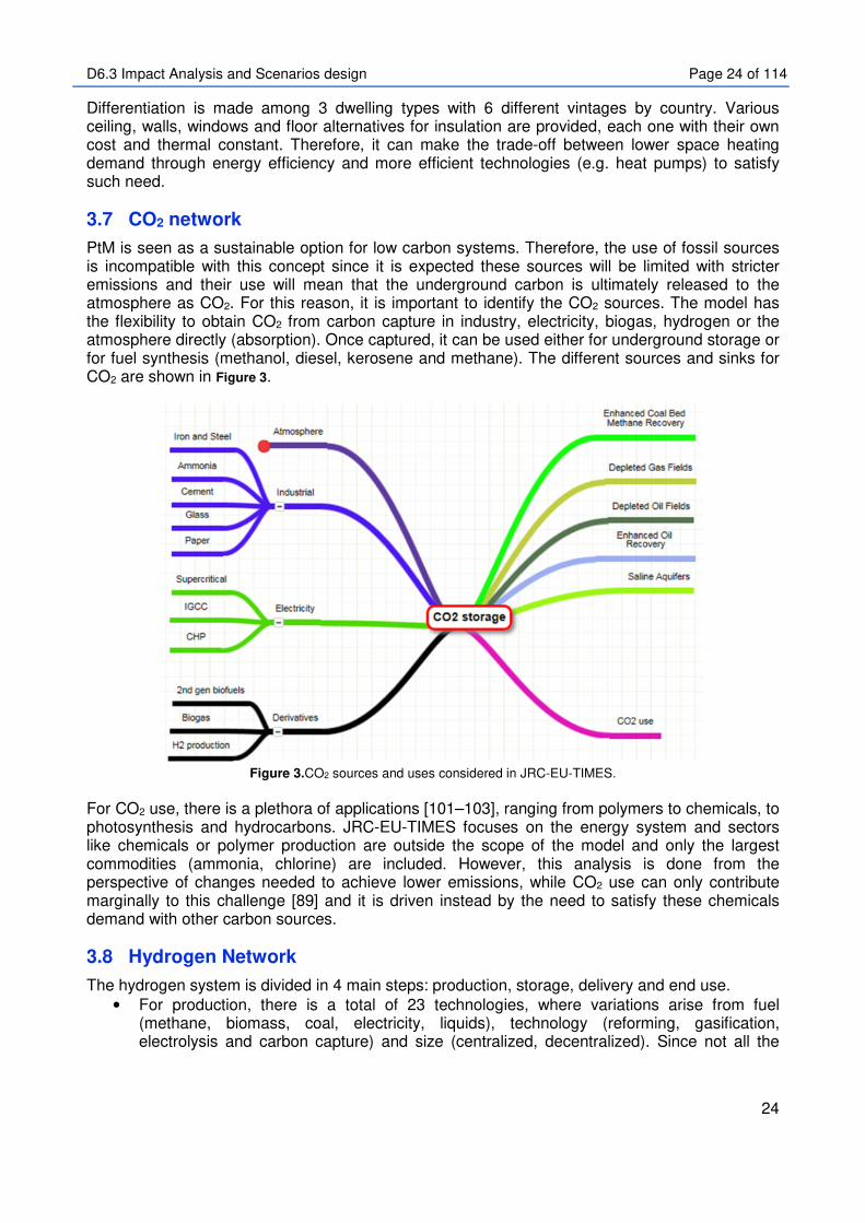
PtM is seen as a sustainable option for low carbon systems. Therefore, the use of fossil sources is incompatible with this concept since it is expected these sources will be limited with stricter emissions and their use will mean that the underground carbon is ultimately released to the atmosphere as CO2. For this reason, it is important to identify the CO2 sources. The model has the flexibility to obtain CO2 from carbon capture in industry, electricity, biogas, hydrogen or the atmosphere directly (absorption). Once captured, it can be used either for underground storage or for fuel synthesis (methanol, diesel, kerosene and methane). The different sources and sinks for CO2 are shown in Figure 3.
Figure 3.CO2 sources and uses considered in JRC-EU-TIMES.
For CO2 use, there is a plethora of applications [101–103], ranging from polymers to chemicals, to photosynthesis and hydrocarbons. JRC-EU-TIMES focuses on the energy system and sectors like chemicals or polymer production are outside the scope of the model and only the largest commodities (ammonia, chlorine) are included. However, this analysis is done from the perspective of changes needed to achieve lower emissions, while CO2 use can only contribute marginally to this challenge [89] and it is driven instead by the need to satisfy these chemicals demand with other carbon sources.
3.8 Hydrogen Network
The hydrogen system is divided in 4 main steps: production, storage, delivery and end use. • For production, there is a total of 23 technologies, where variations arise from fuel
(methane, biomass, coal, electricity, liquids), technology (reforming, gasification, electrolysis and carbon capture) and size (centralized, decentralized). Since not all the

D6.3 Impact Analysis and Scenarios design Page 25 of 114
25
combinations are possible or economically attractive (e.g. electrolysis with CCS or coal gasification for decentralized application), it results in 23 options included. The techno-economic parameters can be found in [67]. The model did not include PEM (Proton Exchange Membrane) electrolysis, but this was added as part of this study. For data used, refer to Appendix 2.
• For storage, there are 3 alternatives: underground storage, centralized tank and distributed tank. The production technologies connected to underground storage are the ones applied at large scale or corresponding to a medium size of a conventional technology. Centralized tank is used for relatively unconventional technologies (e.g. oxidation of heavy oil) and smaller scale production.
• For delivery, there are different pathways that can be followed, including: compression, transmission, natural gas blend, liquefaction, road transport, ship transport, intermediate storage, distribution pipelines and refueling stations (L/L, L/G, G/G). Not all combinations among these are possible (e.g. liquefaction and gas-gas refueling station or liquefaction and injection to the grid) and this results in 20 delivery chains considered. For the reasoning in selection, refer to [104]. Delivery cost for transport ranges from almost 1 €/kg to 6 €/kg. The most expensive steps are refueling (up to 3.8 €/kg) and distribution (3 €/kg). The simplest pathway is blending which covers compression, storage and transmission (~1 €/kg). See Appendix 2 for more details.
• In terms of end use, the hydrogen can be blend with the natural gas (up to 15% in volume) and end up in any of the applications of this commodity, used in the residential sector to satisfy part of the space heating demand (µCHP), industry (steel), transport (cars, buses, trucks) or be used for fuel synthesis (combined with CO2). For blending, 10% is already possible in some parts of the system [105] and the impact of using higher concentrations has also been assessed [106]. Looking at a 2050 time horizon, it is expected that this is de-risked, but 15% is chosen to avoid overreliance on the alternative.
A representation of these different steps is shown in Figure 4.
Figure 4. Structure of the hydrogen supply and delivery chain in JRC-EU-TIMES.

D6.3 Impact Analysis and Scenarios design Page 26 of 114
26
3.9 Sectorial use of hydrogen
Hydrogen in the residential sector can be supplied by 4 pathways: centralized hydrogen with underground storage or tank, decentralized production and by blending with natural gas. Hydrogen can be used directly to satisfy space heat demand through a PEM or SOFC fuel cell (µCHP) to satisfy both power and heat or blend with natural gas and satisfy the same need with existing technologies. This represents an improvement introduced in this study, where the previous version only counted with a burner to satisfy space heating demand. For the specific data, refer to Section 5. In the EU, steel represents 4.7% of the CO2 emissions [107]. Improvements for the industry are divided in two categories: enhanced operation and upgrading of current assets (e.g. process control, heat integration, gas recovery, insulation, monitoring) and technology changes (Corex/Finex iron making, MIDREX, EnergIron/HYL, Direct Sheet Plant (DSP) and CCS) [108]. The two most relevant improvements for this study are the possible use of CCS (which could provide CO2 for possible use downstream) and hydrogen as reduction agent (e.g. MIDREX process) [107]. The overview of the process and technologies included is shown in Figure 5.
Figure 5. Technology coverage of steel industry in JRC-EU-TIMES.
Processes where CCS can be applied are COREX and the conventional blast furnace. The finishing processes (e.g. hot strip, mills, annealing and coating) are clustered in a single process that is common for all routes except for hydrogen (which cost already includes this step). Besides the centralized tank option for hydrogen highlighted in Figure 5 as hydrogen source, it can also be provided by a byproduct stream of the chlorine process. However, in terms of order of magnitude, that flow is not nearly enough to satisfy the hydrogen demand needed in case steel shifts to hydrogen. It has been shown [109] that direct reduction with hydrogen is the technology with the largest CO2 reduction potential in steel, in spite of resulting in a net increase of energy demand. As can be seen from Figure 5, the direct reduction process allows transforming the iron ore to produce steel and satisfy demand. This does not mean that the complexity of the process is lower than conventional, but instead that the parameters (efficiency and cost) chosen to represent the process cover the entire value chain from oxidation, to crude steel production and finishing.

D6.3 Impact Analysis and Scenarios design Page 27 of 114
27
Hydrogen can also be used for refineries and ammonia production, which currently are 2.1 and 3.6 mtpa of the 7 mtpa EU total demand [110]. Part of the hydrogen in refineries comes from internal processes (catalytic reforming), that needs to be supplemented by additional production with methane reforming [111], while for ammonia reforming is the step where is mixed with Syngas to introduce the nitrogen in the process. For refineries, hydrogen production can be disaggregated from the rest of the processes discounting the equivalent natural gas that would be used. Data from [112] was used for refineries, which contains the hydrogen demand per country. For ammonia, using pure hydrogen requires changing the process configuration by eliminating the reforming step and adding an ASU (Air Separation Unit) to obtain the nitrogen. Techno-economic data was taken from [113], energy consumption for the combined process (NH3 conversion, compression and cooling plus ASU) is 0.39 kWh/kg NH3 leading to a hydrogen requirement of close to 190 kgH2/ton NH3. Cost assumptions include that the ammonia section represents around one third of the plant cost and a specific Capex of 140 $/ton. To put these numbers in perspective, cost is almost half of the conventional process (260-285 $/ton) and energy flow of hydrogen is around two thirds of the energy input of gas required by the conventional process (due to reforming efficiency).
3.10 Electricity Network
The relevance of this component for PtM is that electricity storage competes in some cases with network expansion. In places with line congestion and high VRE, an alternative to curtailment or grid expansion is to transform the power surplus to gas and use the capacity available in existing gas infrastructure. Even though the model does not include the spatial network within a country, it does consider its cost and corresponding investment needed in case there is a larger power demand. This introduces an additional cost penalty in case the electricity demand increases, but it does not account for line congestion. For this, a similar approach as for the gas network was followed. Electricity prices were taken from Eurostat for industrial (IE Band: 20-70 GWh) [114] and domestic (DC Band: 2.5-5 MWh) [115] consumers discounting the taxes and levies. Using the electricity demand, the total annuity for investment was calculated. This cost is divided by the installed capacity of the base year to calculate the specific investment cost (€/kW). The network is divided in voltage levels, each sector (users) is assigned to a voltage level and the network cost (resulting from a demand increase in a specific sector) is assigned to the capacity needed (GW) to satisfy such demand. This allows considering the network cost as electricity demand increases in spite of not having the explicit grid representation. Nevertheless, the expansion of electricity infrastructure faces not only financial and technical hurdles but also headwind from municipalities and population, solutions are expected to follow other criteria than cost only. During the summer peak time slice, the capacity factor for PV is 0.8, which corresponds to the maximum PV output and ensures that the system is designed to handle this peak either by curtailment, increasing the investment in the grid or any of the other flexibility options. An additional constraint is the target of 15 % interconnection between EU countries to be achieved by 2030 [116]. For more details on the approach and values used refer to Appendix 5.
3.11 Power surplus estimation
In the present and coming years, PtM is meant to use only power surplus as input due to (1) PtM only has lower CO2 emissions than natural gas in cases where the carbon footprint of the electricity used is low (< 50 gCO2e/kWh) [9–12]; (2) PtM provides flexibility to compensate for VRE variability. In the future, this situation can change since PtM demand can become so large that it cannot operate anymore only with surplus. At the same time, the electricity CO2 footprint is expected to decrease, resulting in a larger number of hours where it is attractive for PtM. In such scenario, PtM could operate instead as part of the demand. It will be one of the last users to satisfy since it counts with large scale storage and can adjust and follow electricity production.

D6.3 Impact Analysis and Scenarios design Page 28 of 114
28
To ensure computational tractability, not all the 8760 hours in a year are used. To simplify the problem, hierarchical clustering is used taking advantage of recurrent hourly, daily and seasonal patterns [117]. Even though this method does not perform as well as other clustering algorithms [118], it allows maintaining the chronological sequence of importance for storage calculations. A day (11 hours), night (12 hours) and peak (1 hour) time slices are used for each season, leading to 12 time slices. The range of hours that they cover is from 77-1428 hours. Within a time slice, there is variable capacity factor for VRE. To account for this, a correlation relates the surplus to VRE penetration and each time slice is sub-divided in two (with and without surplus). VRE penetration and system costs can be estimated with 12 time slices [119], while still avoiding a large increase in calculation time. This approach can lead to deviations due to the smoothening of the shape of the profile [117]. To deal with this, summer peak uses the maximum PV output (80%), while winter peak considers zero contribution from VRE combined with 10% higher demand, ensuring is enough capacity adequacy for sustained periods of no wind and solar. Energy balances are satisfied within a time slice and can be transferred across time slices with storage (daily and seasonal). Within a time slice there will be a variable capacity factor because variations in VRE are faster than the length of the time slice. To account for this, an additional equation is introduced based on VRE and demand (both in energy terms) to estimate the surplus. An additional consideration is that other technologies cannot ramp up as fast to compensate for low VRE contribution. Once surplus is calculated, it can be used for DSM, storage, PtX or curtailed. For more details on this, refer to Appendix 6. Capacity factors for wind and solar are calculated considering the time slice definition provided before (4 seasons, day of 11 hours, night of 12 hours and 1-hour peak) using data for 2010. To reduce dependence of the results on this reference year, summer and winter peaks ensure there is enough capacity to deal with both a surplus (high capacity factor for PV) and a shortage (no VRE contribution) combined with a (10%) higher demand. Therefore, a different reference year will only have an impact over the operational costs, but not on the capacity installed. This covers the two periods (low and high VRE contribution leading to back-up capacity and potential curtailment) that have been identified as the most important in clustering algorithms [118]. Electricity demand is an endogenous variable resulting from its use among the end services.
3.12 Other flexibility options (storage and DSM)
The JRC-EU-TIMES model considers storage solutions that can store energy produced in one time slice and make it available in another time slice in form of either electricity or heat. Therefore, storage is the link between day and night time slices, but also seasonal (only batteries cannot cover seasonal). The technologies covered are: compressed air energy storage (CAES), pumped hydro, hydrogen conversion and batteries (lead acid, Li-ion, NaS, NaNiCl) and thermal (low temperature and underground). Batteries of electric cars are also included with different charging modes. Each technology is represented with two different processes, one for the energy component and one dummy component for the power capacity (same process for charging and discharging, but where the amounts of each operation can be segregated). For thermal storage, the commodity stored is directly heat leading to interaction with the electricity system through allowing a more flexible operation of CHP and gas turbines (when gas is used for heating). For the representation and technologies covered in the model, refer to Appendix 6. Surplus has so far been calculated for an entire time slice and in energy terms. This would imply that the storage has to be large enough to manage the entire surplus over the time slice. Nevertheless, the storage might operate in an hourly/daily mode, which would mean a much smaller energy capacity for the storage. Based on this, additional equations are introduced. One to convert the time slice surplus to daily surplus (using the shortest duration of a season, which

D6.3 Impact Analysis and Scenarios design Page 29 of 114
29
would result in the maximum daily amount) and one for obtaining the power capacity (based on energy/power ratio which is different for each technology and covered in Appendix 1). PtM has the advantage over the above technologies that it can serve as a vector between sectors and that it can provide a different commodity other than power back to the system. In fact, this should be its primary use, given that it has been demonstrated [120–122] that the value of storage rapidly decreases after usually 8-12 hours of equivalent storage capacity (ratio between energy and power rating). Since PtM can provide storage capacity for months, it would fall in the area where the marginal value of every additional hour of storage is negligible. Even though once the gas is produced, it could end up in any of the gas uses (including power), this should be avoided to maximize value. For DSM, it is assumed that a fraction of the demand can be satisfied within the same time slice at no cost (assuming the cost corresponds to the IT infrastructure and associated software development, which is considered negligible compared to the costs in other parts of the system). DSM constitutes one of the options to manage the available electricity surplus (see Figure 19). The fraction that can be shifted depends on the sector (25 % for water heating, 15 % for space heating and 10 % for space cooling, these categories are for electricity consumption in residential and commercial sectors) [123]. DSM in industry is only taken in scenarios with high DSM potential to avoid overreliance in the flexibility option. The fraction that can be shifted is 10% for aluminum and chlorine, 15% for paper and 25% for cement and steel.
3.13 Transport fuels
The transport sector is divided in road transport, aviation and navigation. Road transport in turn is divided in sub-sectors and can be satisfied with different fuels, while the fuel choices are much more limited for aviation and navigation. The combination of fuels that can be used in each transport sector is shown in Table 4, while the alternative intermediate carriers and conversion processes to the produce the fuels are shown in Figure 6. For specific considerations for this section, as well as fuel shares refer to Appendix 1.
Table 4. Combination of fuels use by transport sector.
Gaso
lin
e
Die
se
l
Heav
y
fuel o
il
Jet
fuel
CN
G
LM
G
LP
G
Eth
an
ol
2n
d g
en
b
iofu
els
Ele
ctr
icit
y
H2
Bus x x x x x x x Light Duty x x x x x x x Heavy Duty x x x
x
x x
Car x x x x x x x x Aviation x x Navigation x x x x
It was decided not to include potential carriers for aviation like hydrogen, given that in spite of the vast research that has been in the topic [124–127], its maturity is still too low to rely on it as possible low carbon solution. Furthermore, at this point, there is high uncertainty in the cost and efficiency figures and even though assumptions could be taken for these values, risks associated to technology deployment, performance and learning curve effect are more difficult to capture19. 19 This could be done by changing the interest rate, but it would still require a sensitivity of the technology deployment with different rates, which is still not directly risk

D6.3 Impact Analysis and Scenarios design Page 30 of 114
30
Figure 6. Technology pathways for fuel production and use for final demand.
Similarly, for navigation, several options have been studied, including hydrogen, batteries, anhydrous ammonia, compressed air and liquid nitrogen, wind, solar and nuclear powered [128], but it was decided not to include these. LNG is also an alternative quickly arising for navigation in EU and where efforts are being done to close the gaps in regulatory framework to enable the use of LNG and develop the required infrastructure [129]. However, this seems to be driven by a benefit in sulfur emissions and a stricter regulation [130] rather than having CO2 emissions in mind. It could be detrimental since it would create a lock-in effect given that the facilities will be developed in the coming years making the use of LMG more attractive in the future. For both sectors, there is a large contribution (50-75%) from changes in operations, mechanical design, materials and aerodynamics to CO2 emissions reduction that are not captured as part of the current model, so there is an overreliance in fuel switch, which in reality might be lower than what the model predicts.
3.14 Biomass network and potential
In Figure 6, it has been shown that for low carbon systems (without fossil fuels and refineries) the choices left in the model are limited. Aviation can only be satisfied with PtL (“electrofuels”) [131] or synthetic fuels, navigation will shift to diesel (since fuel oil would lead to positive emissions). There are three different sources: biofuels, synthetic fuels and PtL. From these, biomass not only competes with the other technologies for transport, but can also be used in other sectors. Therefore, use of for example energy residues for hydrogen production is in competition (same raw material) with its use for ethanol production (in road transport). Because of this, it is also important to know the types of biomass included and their possible use in different sectors. This is shown in Figure 7, which includes non-transport use of biomass.

D6.3 Impact Analysis and Scenarios design Page 31 of 114
31
Figure 7. Biomass sources (left) and sinks (right) covered in JRC-EU-TIMES.
Some notes to bear in mind are:
• Starch and sugar can only be used for ethanol production, while rapeseed is the one that can be used for hydrotreated vegetable oil (HVO). Therefore, for starch and sugar there is no competition with either other fuels or sectors. The choice is only if the pathway should be used and to what extent.
• Wood products can also be used for biogas production (not shown in the diagram) and satisfy demand on the cement sector (which otherwise could not be satisfied).
• Common uses are applicable for biogas, biosludge, municipal waste and wood products, but not for agricultural crops.
The potential is between 10 and 25.5 EJ/year for EU28+ by 2050. This is based on [132] and in agreement with previous studies (6.2-22.1 [133], 18.4-24 [134] EJ/year). Most (>85%) of the biomass has a cost below 5 €/GJ. The ones above this cost are rape seed and starch (17 and 21.9 €/GJ respectively), which can only be used for 1st generation fuel biofuels and ultimately imply gasoline production for blending downstream. Around half of the biomass potential falls in the forestry source and could be used for 2nd generation biofuels. Although, it has the largest absolute potential, it is in direct competition with uses for electricity, heating, industry and hydrogen. On the other hand, agricultural crops are one quarter of the potential, but could be used directly for ethanol with no competition for other sectors besides transport. For the specific values refer to Section 5.6 and for assumptions with respect to land use, logistics, heating value, scope of each category, potential by country, refer to [132].

D6.3 Impact Analysis and Scenarios design Page 32 of 114
32
4 Key policies
This section explains some of the key policies that will have an influence on the modeling outcome. Note that the model contains over 300 constraints, which will define the results. However, in this section only the ones that are considered to have the widest impact are explained. In terms of interaction between policies, the system will achieve all the targets specified. However, it is usually the case that one of them is dominating the rest (i.e. binding). For example, it a 90% CO2 reduction target is set, but only a 10% RES target, most likely the RES target does not affect the system since it is being defined by the CO2 target. Therefore, if the RES target is changed to 11%, there would be no extra cost (and no price) since it probably already satisfies the new constraint.
4.1 Primary Energy Consumption (PEC)
The EU 2030 Energy Strategy20 has three main components: 40% GHG emission reductions compared to 1990, at least 27% share of renewable energy consumption and at least 30% of energy savings compared to the business as usual scenario. This constraint related specifically to the reduction in energy consumption. On 30 November 2016 the Commission proposed an update to the Energy Efficiency Directive21, including a new 30% energy efficiency target for 2030, and measures to update the Directive to make sure the new target is met. The implementation of this policy is done by adding up all the gross energy produced to satisfy the energy needs of the system. This includes: fossil, renewable (including biomass) and imports. Reference energy values for the business as usual scenario are taken from [82] and the PEC value for 2030 is almost 56700 Mtoe with 2050 resulting in almost 60000 Mtoe. The effect of this policy is mainly in three aspects: 1. It will promote the use of insulation measures in the residential and commercial sector (50% of the energy consumption in EU [135]); 2. It will promote the use of intermediate technologies with higher efficiency; 3. It will favor energy carriers that imply higher pathway efficiency (i.e. electricity). Note that the first aspect (insulation) is an endogenous choice of the model. It makes the trade-off between additional cost and reduced thermal constant for windows, ceilings, wall and floors considering the different characteristics (type of house, space) and building stock.
4.2 Renewable Energy
Renewables are seen as fundamental to keep EU as global leader in innovation, source of economic growth and jobs for Europeans and access to affordable and clean energy [136]. The goals for RES shares are 20% for 2020 and 27% for 2030. For 2030, a linear trajectory from 2020 targets was chosen by the Commission since it provides more certainty and should help to reduce cost and avoid risks associated with achieving the target. This target includes the breakdown by country since the starting point, cost and potential are different for each one [137]. Setting targets directly for RES can result in a higher system cost since it is already pre-defining the alternative to reach a lower carbon system. If the overall goal is to reach lower GHG emissions (to limit global warming), this should be the one with targets and let the market 20 https://ec.europa.eu/energy/en/topics/energy-strategy-and-energy-union/2030-energy-strategy 21 https://ec.europa.eu/energy/en/topics/energy-efficiency/energy-efficiency-directive

D6.3 Impact Analysis and Scenarios design Page 33 of 114
33
dynamics define the best alternative to reach it. There is an interaction between: RES target, CO2 target and CO2 tax. By setting one, the other two are resultant. For this study, the overall CO2 trajectory is defined and the RES share, as well as the equivalent CO2 price, is obtained as product. For RES share, only the targets for 2020 are included.
4.3 CO2 constraint
This includes all the CO2 emissions of the system, including: residential, commercial, industrial (including chemicals), electricity, intermediate conversion (e.g. refineries), supply, extraction and mining, transport and agriculture. It does not include the emissions for: construction and decommissioning and related to mining and manufacturing activities for imported commodities. The policy includes the target of 40% reduction by 2030 and the ambition of 80% reduction by 205022. An intermediate target of at least 60% by 2040 is also considered in the EU strategy. For a more ambitious target (95%), it is still unclear what the optimal path will be. However, since there might be delays in implementation once the relatively cheap changes in the system are achieved, there could be incentives to consider an accelerated path (which considers such delay). Figure 8 reflects the trajectories followed to reach the CO2 targets by 2050.
Figure 8. CO2 trajectory to 2050 for different targets.
The “Base” trajectory was chosen for 95% to avoid overestimating the rate of change (i.e. a 95% CO2 reduction target in the proposed timeline is already by itself ambitious enough and it would be too optimistic to assume such change can be achieved in an accelerated manner). BAU (Business as usual) considers no major improvement after achieving 2030 goals.
4.4 Emission trading system (ETS)
ETS is a cap and trade system where an overall upper bound is established and companies can trade among themselves the allowances for emission. Companies will implement changes that
22 https://ec.europa.eu/clima/policies/strategies/2050_en

D6.3 Impact Analysis and Scenarios design Page 34 of 114
34
are cheaper than the price of the allowance and as these become more restricted its price (and corresponding changes that can be done) increases. The EU ETS covers approximately 11,000 power stations and manufacturing plants in EU28+, as well as aviation activities. In total, around 45% of GHG emissions are regulated. It remains the world’s biggest emissions trading market, accounting for over three quarters of international carbon trading. The European Commission presented in July 2015 a legislative proposal on the revision of the EU ETS for its next phase (2021-2030), in line with the EU’s 2030 climate and energy policy framework. The proposal aims to reduce EU ETS emissions by 43% compared to 2005. The overall number of allowances to decline at an annual rate of 2.2% from 2021 onwards, compared to 1.74% currently. Since power is covered by ETS and this has some of the lowest costs to achieve a low carbon footprint (compared to e.g. transport or industry), the targets for ETS are stricter than for the overall system. Therefore, an 80% target for the system is equivalent to almost 87% reduction in the activities covered by ETS. This means in net terms, a reduction from almost 2 Gton of CO2 in 2010 to only 0.3 Gton in 2050.
4.5 Effort sharing decision (non-ETS)
This covers most of the activities not included in the ETS system (i.e. transport, buildings, agriculture and waste). Different from ETS, the target is less ambitious (10% overall EU reduction by 2020 compared to 1990) and also allows for increase in emissions for some countries (it ranges from 20% reduction to 20% increase) since it is based on the relative wealth gap (GDP per capita). Another difference is the level of EU coordination, while ETS ensures that allowances can be traded among countries, achieving the ESD target, specific policies and actions are left to each Member State. The model includes the targets for 2020 and a calibration based on EUCO30 for 2030. For a non-ETS sector like transport, another relevant policy is the targets for emissions and efficiency from passenger cars. For 2021, the target is 95 gCO2/km, which translates to 4.1 L/100 km for petrol and 3.6 L/100 km for diesel23. These are also implemented in the model and also considering a further reduction to 70 gCO2/km by 2030.
4.6 Nuclear energy
Representation of nuclear power plants in the model
Each individual existing and planned nuclear power plant in Europe is modelled at reactor level, considering its technological characteristics (efficiency, capacity, historical availability factors, exact start and decommissioning dates). Investments are possible (depending on the scenario) in specific projects or generic projects. Specific projects are modelled one by one and have specific technology data (earliest commission date, installed capacity, efficiency, etc.), whereas the generic projects are modelled on the country level, have a total possible capacity and common technology data. This approach differs from conventional power plants, which are always represented in blocks of plants (like the generic nuclear plants). Each block has performance factors averaged within a
23 https://ec.europa.eu/clima/policies/transport/vehicles/cars_en

D6.3 Impact Analysis and Scenarios design Page 35 of 114
35
certain region and vintage block (decade) and a life dependent degradation of efficiency and life fixed operation and maintenance costs. The nuclear fleet, including the replacement of plants due for retirement, is modelled on its economic merit and in competition with other energy sources for power generation except for Member States with legislative provisions on nuclear phase out. Several constraints are put on the model such as decisions of Member States not to use nuclear at all (Austria, Cyprus, Denmark, Estonia, Greece, Ireland, Latvia, Luxembourg, Malta and Portugal) and closure of existing plants in some Member States according to agreed schedules (e.g. Germany). Nuclear investments are possible in all the other countries.
Existing nuclear fleet representation
The nuclear data for each power plant covers the net installed capacity in MW, the thermal efficiency and the date of beginning commercial operation. The data is taken from the PRIS database of IAEA24, plant operators, Member State nuclear regulators and industry organizations such as the World Nuclear Association.
Lifetime assumptions for the existing nuclear park
The model makes use of nuclear power plants as long as (i) this is economically favorable compared to closing and investing in alternative supply technologies and (ii) the nuclear plant does not reach the end of its lifetime. The JRC-EU-TIMES implements scenarios based on technical and political assumptions for the maximum plant lifetimes. These vary depending on the Member State:
• Explicit end of operation dates are used for member States in which a phase out policy is in place (BE, DE and, to a degree, CH) or that explicitly state the end of a license (NL). Fixed closure dates are also applied to selected power plants in other Member States in which operators have indicated to close nuclear power plants for economic reasons (reactors Ringhals 1,2 and Oskarshamm 1,2 in Sweden). According to the goal to limit the French nuclear capacity at 63.2 MW25, it is assumed that the two units at Fessenheim cease operation in 2017. End of life dates for the existing UK fleet have been taken from the operator's (EDF ENERGY) publication as these exceed the current regulatory period. Finally, this option has been applied to power plants which have been decommissioned in the time period between the base year for the model calibration and today.
• Generic reactor lifetimes are used in all other cases assuming that the operators of existing reactors will be able to renew their operating licenses. Technical lifetimes of up to 60 years are envisaged by most nuclear operators and possible in the most ambitious scenario. Taking into account that licenses might not be prolonged for political reasons, scenarios with shorter reactor lifetimes have been prepared.
Figure 9 shows the installed capacity of the current nuclear fleet as a function of time for three different scenarios, differentiated by the maximum lifetime of the existing nuclear power plants. Fixed closure dates remain the same in all scenarios.
24 https://www.iaea.org/pris/ 25 http://www.developpement-durable.gouv.fr/Renforcer-la-surete-nucleaire-et-l,41397.html

D6.3 Impact Analysis and Scenarios design Page 36 of 114
36
Figure 9. Development of the capacity of the currently installed nuclear power fleet in the EU.
For PtM scenarios, 40 years is used including the option of reinvestment for a 20 years plant lifetime extension to bring this life to 60 years.
0
20
40
60
80
100
120
140
160
2010 2015 2020 2025 2030 2035 2040 2045 2050
[GW
]
Remaining installed nuclear capacity
Remaining Capacity
(40 yrs scenario)
Remaining Capacity
(50 yrs scenario)
Remaining Capacity
(60 yrs scenario)

D6.3 Impact Analysis and Scenarios design Page 37 of 114
37
5 Assumptions and data
5.1 PtM performance
For the methanation step, there was a wide range of values found in literature (especially for cost), where it is difficult to identify in some cases the specific elements that are included in the cost estimate (e.g. engineering, installation, construction) and even in some cases the reference for the cost (e.g. kW of H2 input vs. kW of methane output). To tackle this uncertainty a set of values is defined to be used in the base scenario and also an optimistic performance is identified to establish the upper bound for the role of the technology. Techno-economic parameters for methanation are shown in Table 5.
Table 5. Base and extreme techno-economic parameters for methanation.
Year Capex [138–140]
Fixed Opex26
Variable Opex27
Efficiency28 Availability Factor29
Lifetime
/€/kW /€/kW /€/kWh /Years
Base
2015 750 [7] 37.5 - 0.75 [29] 0.95 25 2020 600 30 0.78 0.95 25 2030 450 22.5 0.81 0.95 25 2050 250 [141] 12.5 0.85 [140] 0.95 25
Min
2015 175 [142] 5.25 0.83 [143] 0.95 30 [28] 2020 150 4.5 0.85 0.95 30 2030 125 3.75 0.87 0.95 30 2050 7530 [140] 2.25 0.9031 0.95 30
Max
2015 1500 [144] 112.5 0.60 [145] 0.85 [140] 20 [6] 2020 1350 101.3 0.65 0.85 20 2030 1000 75 0.70 0.85 20 2050 700 [6] 52.5 0.75 0.85 20
5.2 Hydrogen Network
Total costs for each of the pathways results from cost aggregation of the individual steps. The specific cost for each of the steps is shown in Table 6, while its combination in the selected pathways for transport and resulting hydrogen production cost is shown in Figure 10 for 2025 (same values assumed for 2050). Note that for the other sectors, the pathways mostly constitute of compression, transmission, distribution and underground storage, with the cheapest option (at 1.1 €/kg) being the blending in the natural gas network (as expected), since it eliminates an expensive steps (i.e. distribution).
26 Range is from 3 to 7.5%, as a fraction of the Capex from [17][18] (excluding CO2 cost) 27 Most of the variable cost is the CO2 source 28 Efficiency is expressed as energy output (methane plus heat recovered, if any) divided by the energy input (contained in the hydrogen) 29 The reactor itself usually has limited trip initiators (related to temperature control). Most of the trip in the system impacting the availability will occur elsewhere in the system (e.g. compressors) 30 Biological methanation is cheaper and assuming a capacity of > 3 MW per unit 31 Assuming part of the heat released is recovered as steam

D6.3 Impact Analysis and Scenarios design Page 38 of 114
38
Table 6. Contribution of individual conversion steps to final hydrogen production cost for 2025.
Step Cost (€/kg)
Compression 0.10 Transmission pipeline 0.49 Liquefaction 1.19 On site liquefaction 8.50 Road Transportation Short 0.04 Distribution pipeline 3.04 Refueling Liquid to Liquid 1.18 Refueling Liquid to Gas 3.39 Refueling Gas to Gas (large) 1.00 Refueling Gas to Gas (small) 3.81 Underground Storage 0.33 Gas Storage Bulk 1.22 Local Gas Storage Bulk 2.18 Liquid Storage Bulk 0.28
Figure 10. Capex contribution to hydrogen production cost for transport pathways.
The model does not capture the spatial distribution of supply and demand. Therefore, the steps assume a specific configuration for each step. For example, a transmission pipeline is 0.1 m in diameter and 500 km of length, while a distribution pipeline assumes an 8-cm pipeline. For more critical items like refueling stations a range of scales (300 – 2500 kg/d) was considered, as well as different delivery modes (gas or liquid). For more detail, refer to [67,104]. In the hydrogen system, two additional production technologies were added, namely PEM (Proton Exchange Membrane) and SOEC (Solid Oxide Electrolysis) [146,147,140,148]. Advantages of the former include faster response, high voltage efficiency, higher current densities at the expense of (current) higher cost and shorter lifetime than AEL. SOEC enables a step increase efficiency. It operates at high temperature (800-1000 ºC). This allows reducing the free Gibbs energy and in turn the cell voltage (0.9-1.3 v for SOEC vs. 1.8-2.4 v for AEL), which decreases the electricity consumption of the cell. It also has the potential for co-electrolysis of water and CO2 directly to Syngas. Both of these complement AEL (Alkaline) in electrolysis, while expanding the list of possible hydrogen production processes to 24. The data for PEM was found to vary significantly due to the high uncertainty associated to learning curve and possible deployment in the future.

D6.3 Impact Analysis and Scenarios design Page 39 of 114
39
Therefore, the minimum and maximum values found were chosen with the objective to understand the impact of extreme expected techno-economic parameters. These are shown in Table 7. For SOEC, values from DoE were used [149] (Table 8), which reflects a performance better than the “Optimistic” scenario for PEM.
Table 7. Base and extreme techno-economic parameters for hydrogen production with PEM.
Year Capex [138–140]
Fixed Opex32
Variable Opex33
Efficiency34,35 Availability Factor
Lifetime
/€/kW /€/kW /€/kWh /Hours
Base
2015 1500 45 - 0.65 [150] 0.95 25000 2020 1200 36 0.70 50000 2030 950 [151] 28.5 0.75 60000 2050 750 22.5 0.80 80000
Min36
2015 1200 18 0.7 [151] 0.91 [152] 50000 [151]
2020 900 13.5 0.75 60000 2030 650 9.75 0.8 80000 2050 400 [6,153] 6 0.86 [151] 105
[154]
Max
2015 2000 [138] 100 0.6 [138] 0.97 [153] 30000 2020 1800 90 0.65 35000 2030 1400 70 0.7 [138,153] 40000 2050 1000 [140] 50 0.75 [155] 50000
[154]
Table 8. Techno-economic parameters for hydrogen production with SOEC.
Year Capex [138,140,139]
Fixed Opex37
Variable Opex38
Efficiency39,40 Availability Factor
Lifetime41
/€/kW /€/kW /€/kWh /Years
2020 785 66 0.905 0.95 2 2030 450 13.5 0.949 0.95 10 2050 300 9 0.95 20
32 Range is from 1.5 to 7%, as a fraction of the Capex from [6][12][13] (excluding electricity) 33 Main variable cost is based on electricity price, which is endogenous for the model 34 Efficiency expressed as energy in the product vs. energy in the feed (MWout vs. MWin in LHV terms) 35 Efficiency refers to stack efficiency with small loses (e.g. dryer, control and auxiliary equipment) not included 36 Min/Max actually refer to an optimistic and pessimistic set of assumptions (where optimistic includes the best efficiency values combined with a low cost, that do not necessarily translate to the lowest values in all categories) 37 Taken as 3% of the Capex 38 Main variable cost is based on electricity price, which is endogenous for the model 39 Efficiency expressed as energy in the product vs. energy in the feed (MWout vs. MWin in LHV terms) 40 Efficiency refers to stack efficiency with small loses (e.g. dryer, control and auxiliary equipment) not included 41 Current limitation is the stack lifetime, due to the high degradation rate and lower efficiency after only 4000-5000 operating hours

D6.3 Impact Analysis and Scenarios design Page 40 of 114
40
5.3 Sectorial use of hydrogen
Hydrogen can be used to satisfy heat and power demand in the residential and commercial sectors. This can be done directly with hydrogen or through a blend with methane and use of existing infrastructure, using CHP as end use technology. Techno-economic parameters of these technologies in 2050 are shown in Table 9. Table 9. Techno-economic parameters for hydrogen use in residential and commercial sectors [156].
Sector Feed Technology Investment Variable Opex
Efficiency Heat to power ratio
Life-time
/€/kW /€/GJ /years
Residential
NG blend PEM 9000 5.0 0.39 1.46 20 NG blend Solid Oxide 3964 4.8 0.50 0.88 20 Pure H2 PEM 9000 6.7 0.50 0.96 20 Pure H2 Solid Oxide 3000 4.5 0.55 0.78 20
Commercial NG blend PEM 4000 12.5 0.39 1.33 20 NG blend Solid Oxide 1850 2.2 0.60 0.57 20 Pure H2 Solid Oxide 350 5.6 0.50 0.9 20
A major difference between both sectors is the economies of scale. Deployment in the residential sector is usually linked to a size of 0.3-1 kW, while commercial deployment can be up to 1 MW. To put these numbers in perspective, currently, the order of magnitude for investment is 7500 €/kW for commercial applications [157,158] and 15000 €/kW for residential [151,157]. The largest deployment has been in Japan as part of the EneFarm project, where 120000 devices have been deployed since 2009 with subsidies up to 15000 $/unit [151] with an observed cost reduction from 50-70 k$/kW (with the higher price being associated to lower production volumes) to 20 k$/kW was observed in this time span. Based on the latest estimate [159], the learning rate for this technology is around 16%, where the fuel cell stack has a higher learning rate (20.5%) than the balance of the plant (12%). Considering a base price of 32 k$/kW and an initial capacity of 10000 units, reaching a deployment of 1 million units would drive the cost down to 10 k$/kW and to reach a relatively low (3500 $/kW) cost target, a relatively high penetration is required (70 million units, which would represent around 10% penetration in Europe, US and Japan). Hydrogen use in steel covers the entire transformation process from the iron ore to production of the crude steel that goes to the finishing process. The representation is equivalent to the primary conversion step (sintering/pellets), first oxidation step (e.g. blast furnace), production of crude steel (e.g. electric arc furnace) and finishing. Therefore, the cost reflects such scope. Most of the costs for the steel industry were taken from [107], which in turn were taken from the ETSAP technology brief and [160] with additional input from industry experts. Values for hydrogen conversion are in Table 10, while the rest of technologies can be found in Appendix B of [107].
Table 10. Techno-economic parameters for steel reduction with hydrogen [107].
Variable Value Units Input42 – Electricity 0.7 PJ Input – Iron Ore 1.5 Mton Input – Hydrogen 17 PJ Output – Slag for cement 0.25 Mton Capex 400 €/Mton Fixed Opex 10 €/Mtpa Variable Opex 2 €/Mtpa
42 Input and Output are expressed per Mton of steel demand

D6.3 Impact Analysis and Scenarios design Page 41 of 114
41
5.4 Other CO2 uses
There are two main uses for CO2, either for liquids (co-electrolysis and hydrogenation) or to methane. Techno-economic parameters for methanation have been published before. Therefore, this section covers PtL parameters which are shown in Table 11. Table 11. Techno-economic parameters for Power to Liquid technologies in 2030 [161].
CO2 source
Process Product Capex Fixed Opex
Variable Opex
Efficiency Lifetime
/€/kW /€/GJ /€/GJ /Years System Hydrogenation Diesel/Kero 392.1 10.4 0.06 0.780 20 System Hydrogenation Gasoline 849.6* 54.3* 0.10* 0.818 20 System Co-
electrolysis Diesel/Kero 889.8 20.8 0.12 0.546 20
System Co-electrolysis
Gasoline 1873.9* 103.0* 0.22* 0.573 20
Atm Co-electrolysis
Diesel/Kero 3559.2 83.1 0.46 0.333 20
Atm Co-electrolysis
Gasoline 7495.4* 411.8* 0.87* 0.333 20
*Values are for 2025 rather than 2030 To put the Capex numbers in perspective, various references can be used. One is to benchmark the technology across studies. This was done and values are reflected in Table 12. Another one is a competitor technology for liquid production (XTL), where GTL is around 800 €/kW, CTL 1200 €/kW and BTL 1800 €/kW. The other one is another reference for a similar technology (methanol with CO2 from air through electrodialysis) [87], where the assumed Capex was 2430 €/kW for 2050. This shows that the assumed values are conservative and it would require a high CO2 price to select these options. PtL performance was also varied as part of the sensitivities to understand how PtM activity changes. For the values used as sensitivities refer to Appendix 1. Table 12. Benchmark values for techno-economic parameters of PtL (Fischer-Tropsch route).
Electrolysis CO2 source
Liquid route DVGW43 LBST 1 [162]
LBST 2 [87]
VDA [163]
Low temperature
System Capex (€/kW44)
1226.1 993.5 1795.9 -
Efficiency45 (%)
46 53 - -
Air Capex (€/kW) 2127.8 2006.5 3040.8 3198 Efficiency (%) 36 42 39 42
High temperature
System Capex (€/kW) 707.9 819.3 888.9 - Efficiency (%) 63 64 - - Air Capex (€/kW) 1786.3 1786.3 2317.5 2561 Efficiency (%) 47 47 45 48
+ “System” means that the CO2 can be provided by any source meaning industry, electricity, biogas, H2 production, BTL or air
43 DVGW = Deutscher Verein des Gas- und Wasserfaches = German association for gas and water. Values are the collection from various projects where DVGW is involved, but are not part of any publication yet 44 Specific cost per kW of liquid product 45 Electricity input (MW) vs. energy in fuel product

D6.3 Impact Analysis and Scenarios design Page 42 of 114
42
5.5 LMG uses
LMG can be used in ships, buses and heavy-duty trucks. Data for buses and heavy-duty trucks was taken from [164] and it is reflected in Table 13 for heavy-duty and Table 14 for buses. For LMG use in ships, the values of 0.12 and 0.27 gCO2/(ton*nautical mile) (0.12-0.26 MJ/km) were already introduced in Section 3.5. The main uncertainty is not the absolute value, but the difference with diesel/HFO engines. IEA estimates that to stay in a below 2 ºC scenario, efficiency should improve by more than 60% [165]. This means engines will get more efficient in time. However, methane can have the disadvantage that depending on the type of engine used, there might be additional methane leaks that increase the GHG emissions compared to diesel/engine, also considering the potential losses upstream in the compression and distribution system. Based on this, the two efficiency values for ships were chosen to reproduce one case where diesel/HFO is used to satisfy demand and one where LMG is used instead.
Table 13. Investment and efficiency for heavy-duty transport for 2010 – 2050 [164].
2010 2020 2030 2040 2050
Investment /€
Diesel 72857 74113 88075 85376 82945 Electricity 122204 111195 107677 104680 101955 LMG 100786 100518 111169 107339 103785 Hydrogen 497866 418256 179534 149590 137097
Efficiency /MJ/km
Diesel 10.82 9 7.58 7.55 7.52 Electricity 10.07 8.47 7.67 7.61 7.54 LMG 11.9 10.09 8.99 8.95 8.92 Hydrogen 9.17 7.67 7.11 6.62 6.15
Table 14. Investment and efficiency for buses for 2010 – 2050 [164].
2010 2020 2030 2040 2050
Investment /€
Diesel 178571 180038 186906 185121 186964 Electricity 382955 280369 253934 233361 213774 LMG 206176 206051 211633 208615 205797 Hydrogen 403390 357314 235833 219930 212881
Efficiency /MJ/km
Diesel 14.69 12.58 9.97 9.31 8.71 Electricity 5.83 5.32 4.97 4.91 4.86 LMG 16.16 14.19 11.24 10.5 10.46 Hydrogen 10.6 9.61 9.3 8.67 8.05
5.6 Biomass potential
Figure 11a shows the contribution of the main categories to biomass potential. It is evenly distributed across several categories. A factor that plays a role in the use of biomass is the price at which it can be obtained. This is shown in Figure 11b. Almost 86% of the biomass has a cost below 5 €/GJ. However, the two most expensive categories are the ones that could be used for 1st generation biofuel and have no competition for other use (starch and rapeseed).

D6.3 Impact Analysis and Scenarios design Page 43 of 114
43
Table 15. Annual activity limits for biomass sources in 2050 (in PJ/year) [132].
Potential High Reference Low Sugar crop production 1094.6 995.1 995.1 Rape seed production 1136.8 1033.4 1033.4 Starch crop production 313.3 284.8 284.8 Grassy crop production 2527.8 1524.9 952.9 Willow and poplar 600.3 363.8 388.6 Biogas Production 1874.1 1251.3 624.9 Agricultural waste potential 2136.4 1025.5 606.6
Wood products 3211.2 741.5 741.5 Forestry residues potential 6753.3 283.1 283.1
Wood processing residues 1220.7 265.7 265.7
Municipal Waste Production 921.4 736.2 441.9
Industrial Waste-Sludge Production 69.4 52.6 29.8
Sub-total 21859.2 8557.9 6648.3 Imports to EU Import of bioethanol 1982.9 572 165 Import of biodiesel 814.7 469 270 Import of wood products 944 517 283
Figure 11. (a) Biomass potential distribution by type of source. (b) Supply cost curve for biomass

D6.3 Impact Analysis and Scenarios design Page 44 of 114
44
6 Scenario definition
The scenarios for this study should consider: (1) the uncertainty associated to future development of the energy system, therefore covering a wide range of conditions; (2) that the energy system can evolve both in a direction where methanation plays a key role, but also one where its contribution is limited; (3) that the range of possible outcomes needs to be reduced to a couple of representative scenarios to facilitate understanding, communication and use for other tasks. Based on the above, the scenarios used for this study are a combination of normative and exploratory. They are normative given that the system will reach the defined CO2 reduction target (mandatory as constraint for the model since this is linked to achieving a 2 ºC or lower scenario), while they are exploratory for the range of technologies and routes the model has to satisfy such constraint and where the choices in either techno-economic parameters or possible routes available will lead to different possible future systems. The scenarios are not meant to be forecasts on how the energy system will evolve, but instead to shed some light into the effect of the uncertainties and inform decision makers on the robustness of the technology and its potential outlook under different unfolding set of events. These constitute the quantitative part of a scenario analysis [166–170], where the purpose has been mainly to analyze how changes can affect PtM role in a future system. The relation between variables to depict alternative futures and relate them with technical, political, economic, social drivers in a consistent and coherent manner has not been done. No probability has been added to each of the scenarios and no specific intermediate scenarios have been analyzed (e.g. if CCS is not socially acceptable until 2040, by when it is recognized that is a key technology to achieve a low carbon system and becomes deployed) since these will lie within the extremes analyzed. Part of the scenario definition involves the identification of the most influential parameters (on PtM). This ranges from system parameters (e.g. absence of CO2 storage) to technology specific parameters (e.g. PtM Capex). A total of 22 parameters were identified. Combinations of these parameters were made to understand their effect on the system and outlook for the technology. The ones with the largest influence are presented in Table 16Fehler! Ungültiger Eigenverweis auf Textmarke., while the rest are listed in Appendix 7 (which also includes rationale for the selection of the scenario). These parameters were combined leading to over 120 scenarios, out of which 55 were selected (Appendix 7) and their insights are included in Section 7. These scenarios were selected based on previous studies and results during preliminary runs. However, to facilitate understanding of the results, 8 main scenarios are selected for emphasis in the analysis (see Table 16 for more on the assumptions for each parameter):
• Low carbon (2 scenarios). Only CO2 target as constraint and full flexibility for the rest of technologies. The two scenarios are 80 (reference) and 95 % CO2 reduction.
• No CCS (2 scenarios). Same as above two scenarios, but without CO2 underground storage possible. This can be the result of limited social acceptance, a general ban of fossil fuels or limited research on the technology.
• Realistic (1 scenario). Scenario with what is perceived (by the authors) as highly possible constraints that favor PtM. This includes 95 % CO2 reduction, no CO2 underground storage, low Capex (75 €/kW) for methanation step, high VRE potential (see Appendix 2).
• Alternative without PtM (1 scenario). Scenario with a different set of constraints that are also likely, but that do not favor PtM. This aims to show that it is also possible that the system evolves in a direction where PtM plays a limited role. This includes 95 % CO2 reduction, CCS possible, high biomass potential, high VRE potential, high PEM performance, electric heavy-duty transport possible and low LMG efficiency in ships (25 gCO2/ton*nm).

D6.3 Impact Analysis and Scenarios design Page 45 of 114
45
• Optimistic (1 scenario). This covers the most favorable set of conditions for PtM and establishes an upper bound for the technology activity. This includes the set of conditions in the “Realistic” scenario plus low biomass potential, high gas price, high cost for the electricity network, high PtM efficiency, high PEM performance, low PtL performance, SOEC possible and high LMG efficiency in ships (12 gCO2/ton*nm).
• Business as Usual (1 scenario). This is only included to establish a reference for cost (CO2 price) and energy consumption. However, this only achieves a CO2 reduction of 48 % by 2050 and therefore would make more challenging achieving the 2 ºC scenario.
Table 16. Key parameters46 varied across scenarios to identify trends and shifts in the system.
Parameter Explanation Rationale Scenarios
CO2 reduction target47
Emissions target for 2050 expressed as a percentage of 1990 emissions
It is expected that PtM will play a larger role as target becomes stricter since there is limited budget for emissions from gas
• 80 % CO2 reduction* • 95 % CO2 reduction
CO2 storage
Absence of CO2 underground storage (e.g. due to lack of social acceptance)
This has been identified as key option to decarbonize the energy system, specially sectors other than power. Not having CCS will make the need for other technologies larger
• CO2 storage available*
• No CO2 storage
VRE Potential
Higher PV and wind potential (see Appendix 2)
Initial estimates are conservative. If higher potential is assumed, more VRE deployment will lead to more electricity surplus to deal with and a larger need for flexibility where PtM can play a role
• Reference* • Higher potential for
solar and wind from [85,87]
Biomass potential
Refers to the potential available for each category
Biomass can be used in all sectors (where it can compete with gas). Limited potential requires the development of other technologies.
• Reference* (10 EJ/y) • Low potential (6.5
EJ/y) • High potential48 (25.5
EJ/y) PtM Cost Lower Capex for the
technology Tackle uncertainty in cost learning curve and assess how a lower cost can affect its future deployment
• Base performance* • Optimistic (Min values
from Table 5) PtM efficiency
Maximum theoretical efficiency of 100 % (including heat recovery)
Upper bound for technology outlook with best possible performance and production of additional revenue stream
• Reference efficiency (refer to Table 5)*
• 100 % efficiency
PtM Subsidy
Subsidy to promote the technology with 1 €/GJ in 2025, 2 €/GJ in 2040 and 3 €/GJ in 2050
PtM is currently not commercially deployed. Technology might require subsidy to start deployment. Subsidy is chosen to be equivalent to 20-30 % of the gas prices for 2050
• No subsidy • Increasing subsidy
from 1, 2, 3 €/GJ in 2020, 2040 and 2050 respectively)
LMG efficiency in marine transport
There is a factor 2 between the best and worst performers based on current data (12-25 gCO2/ton*nm)
Future performance can further improve and become more efficient (MJ/km) than fossil options. LMG role in transport is evaluated for this scenario
• High (12 gCO2/ton*nm) efficiency*
• Low (25 gCO2/ton*nm) efficiency
46 There are parameters directly associated to hydrogen and PtL, which are discussed (including more detailed data) as part of a separate article (in preparation) 47 There are 3 interlinked variables: RES fraction, CO2 price and CO2 reduction target. This was selected given that the main target is to achieve a low carbon system and the response of the other two variables will depend on the set of technologies and constraints (indirect effect) 48 See Appendix 1 for reference, low and high values including breakdown by category

D6.3 Impact Analysis and Scenarios design Page 46 of 114
46
7 Results First, scenarios are introduced (Section 7.1) by looking at general indicators such as final energy demand, annual system cost (and corresponding CO2 price) and composition of the electricity mix (focus on electricity given it is the largest supply sector). Then (Sections 7.2 to 7.5Fehler! Verweisquelle konnte nicht gefunden werden.), specific parameters for PtM are analyzed, specifically (1) the price of its output (which is an indication of how competitive it is compared to natural gas); (2) gas balance (including sources and sinks); (3) the seasonal use of PtM and (4) the CO2 balance (since PtM should use biogenic sources and to understand how it compares with the other possible CO2 sinks). These two (general and specific indicators) constitute the first objective of this study, while the second one is fulfilled by identifying the drivers and barriers for PtM and how these can be shaped to choose suitable scenarios for subsequent activities (Section 0). Previous studies [7,26,28,31,46,154] have estimated that PtM will only play a role in the system for high CO2 reduction targets, since only then there are adequate hours with low cost and low CO2 footprint electricity, to justify the investment from an economic perspective. This is not expected to occur in the short term. Because of these two reasons, only numbers for 2050 are shown across scenarios. In case PtM is not used in 2050, it is considered highly likely that it will not be part of the system for previous years. Variables like system inertia, market dynamics and politics, among others are not captured as part of the model. Because of these, achieving high decarbonization targets (such as the ones explored in this study) could take longer than foreseen. Therefore, results presented hereinafter are to be understood as bounded to a system with such CO2 reduction rather than linked to the specific 2050 time horizon. The difference between the annual system cost of a specific scenario and the BAU scenario is an indicator for the additional cost of the requirements to the point of an energy system with 80 % or 95 % CO2 reduction.
7.1 Energy, electricity and cost overview for scenarios
This section aims to understand how the low carbon system differs from one with higher emissions and how the different constraints influence the design of this system. Figure 12 illustrates the changes in energy balance with the final energy demand split by energy carrier, while Figure 13 provides insight into the total system cost, sectorial contribution and associated CO2 price. Complementary results are included in Appendix 8.

D6.3 Impact Analysis and Scenarios design Page 47 of 114
47
Figure 12. Final energy demand by energy carrier across main scenarios.
The largest changes across scenarios are in liquid, gas and hydrogen flows. Liquid includes fossil oil-derived products, Fischer-Tropsch, biomass conversion to liquid (BtL) and PtL, this forms a large part of the BAU scenario, with mostly fossil oil. Transport is one of the more difficult sectors to decarbonize, which leads to still using fossils in this sector for the BAU scenario (overall 48 % CO2 reduction). The three largest drops in liquid demand are (1) the shift away from diesel in private transport (where diesel is more than 8500 PJ in the BAU scenario), (2) the shift in heavy-duty trucks (to LMG/hydrogen depending on the scenario), which is a sector that has a demand of 5000 PJ and (3) the shift from fuel oil to LMG in marine transport (demand of 2000 PJ). Gas contribution can be high either when CO2 storage is possible, lower CO2 target is set or for a high biomass potential, when the biomass is used for negative emissions in power and hydrogen and positive emissions can be incurred in the commercial sector with gas. Biomass contribution is small since it is converted to another energy carrier (e.g. electricity or liquid) and the final use of direct biomass without previous conversion is limited (in industrial or commercial sector). Coal is negligible across all scenarios including BAU scenario. There is a progressive electrification as the scenario becomes more restrictive, with up to 50 % of the final demand. Electricity production in BAU is similar to today (3600 vs. 3200 TWh), but it almost doubles with 95 % as CO2 target and up to 11000 TWh with higher VRE potential (see Appendix 8). VRE (wind and solar) can be up to 70 % of the mix when their potential is the highest. BECCS (gasification) plays a limited role in terms of electricity share for scenarios with CO2 storage, given that scarce biomass (10 EJ/year for EU28+) is better used in other sectors and only plays an important role with higher biomass potential (25.5 EJ/year). However, it makes a large difference in terms of CO2 emissions and total electricity CO2 footprint since it can provide up to 180 MtonCO2/year. Electricity generation with fossil fuels using CO2 capture plays a larger role in scenarios with CO2 storage, with its largest contribution at almost 900 TWh. Nuclear and hydro are relatively constant across scenarios regardless of parameters. The electricity sector is the most cost-effective to decarbonize. Because of this, even in BAU scenario (48 % CO2 reduction), the total emissions for power production correspond to around 20 gCO2/kWh, while for

D6.3 Impact Analysis and Scenarios design Page 48 of 114
48
most of the scenarios they are -15 to 0 gCO2/kWh. This is drastically lower than current values, which are close to 350 gCO2/kWh for EU28+ (see Appendix 9). There is a large difference between the generated electricity and final demand since electricity consumption for electrolysis can be up to 40 % of generation (reflected as either hydrogen or liquid in the final energy demand, see Appendix 8). A sensitivity with an additional 200 % for the grid cost decreases total centralized generation by 8 % (from 11100 to 10200 TWh) with limited impact in the electrolysis and industrial capacity (which do not require distribution grid expansion and are less impacted by the assumption), while sectors at the distribution level experienced a 15 % decrease in demand. Nevertheless, part of this is replaced by more decentralized generation with PV that increases by almost 450 TWh. A higher grid cost makes the power system more expensive (+9 %) and also the commercial sector (> +100 %) since the heating needs to be satisfied with µ-CHP and gas, which represent a more expensive option than heat pumps, with a similar effect occurring in the residential sector as potentially positive effects of aggregation of µ-CHP were not considered in this work. Overall, the change results in a system 5 % more expensive (annual costs).
Figure 13. Total annual system cost split by sector and marginal CO2 price. Values represented in Figure 13 are the total annual costs for the energy system in 2050. This includes also energy efficiency measures and actual devices (heat pumps, lighting, stoves, heaters) for the residential sector and the vehicles (cars, buses, trucks) for the transport sector. These can represent around 0.12, 0.3 and 1.8 trillion€/yr respectively from values in Figure 13. Such cost covers 97-98 % of the transport costs in Figure 13 with the remainder represented by BtL and the charging stations for battery electric vehicles (BEV). Scenarios with lower targets use less efficient (cheaper) cars and this results in 15 % lower cost for BAU (compared to 80 % CO2 reduction). Cost in the power sector increase with more restricted scenarios (higher electricity generation) and the fraction (in cost) for the network varies between 15 and 32 % of the total sector cost, with the high value actually corresponding to BAU scenario and decreasing progressively with more restrictions. This corresponds to 105-140 bln€/yr for most of the scenarios (including replacement) compared to around 90 bln€/yr for BAU. A large advantage of low carbon scenarios is the reduction of the import bill. Imports represent around 400 bln€/yr for BAU, which is reduced to around 250 bln€/yr for 80 % CO2 reduction and further to 190 bln€/yr with 95 % CO2 reduction. As the scenario becomes more restrictive, imports are reduced even

D6.3 Impact Analysis and Scenarios design Page 49 of 114
49
further reaching levels below 50 bln€/yr. To put these numbers is perspective, the GDP for EU28 was 15.3 trillion€ for 201749 and expected to be 22.5 trillion€ by 2050 [82]. A low carbon scenario does not necessarily translate into a high CO2 price. For the "Alternative" scenario that combines a high biomass, wind and solar potential, the marginal CO2 price can be only 10 % higher than the BAU scenario (136 vs. 125 €/ton). The largest changes in CO2 prices are the CO2 target, CO2 storage absence and biomass potential. The CO2 target can more than double the price by the individual changes from BAU to 80 % and further to 95 % CO2 reduction. CO2 storage potential has a similar effect of doubling the CO2 price when CCS is not possible. A high biomass potential can actually compensate for the cost increase caused by the lower CO2 target. The rest of the lower CO2 price in the "Alternative" scenario comes from the rest of the changes (higher VRE potential, electric trucks, better PEM performance). The use or not of LMG in the marine transport has a negligible effect on the CO2 price (< 1 % change) and can actually lead to an increase in marginal CO2 price for more restricted scenarios50. The impact is through reallocation of the biomass since marine transport is mainly satisfied with diesel when LMG is not an option. When biodiesel is used, it causes a larger BtL activity and biomass for power and H2 production decreases. The reduction in total costs can be between 0.5-1 % for scenarios with LMG in transport. However, this is mostly associated with the higher efficiency used (0.12 MJ/(ton*km)) compared to diesel engines rather than the specific fuel (LMG). The effect PtM has on marginal CO2 price is 0.5 % when the technology is initially deployed (only lower Capex), 2 % with its higher deployment associated to the higher efficiency and up to 10 % when it is subsidized. Costs for PtM are negligible for the entire system and represent only a fraction up to 0.0005 of the total system cost. This fraction increases to 0.0013 for a high efficiency (combined with 95 % CO2 reduction, no CO2 storage, low Capex and high VRE potential), 0.0014 with cheaper hydrogen (better PEM performance) and 0.0024-0.0025 when either no PtL is used (no other sink for CO2) or “Optimistic” scenario. When compared to the gas supply system51 (import, LMG, storage, without including costs for downstream conversion), the fraction increases to 0.45 % for the “Realistic” scenario and up to 5.7 % for the “Optimistic” scenario. This translates into annual costs of 2.5 bln€ for the “Realistic” scenario and up to 10 bln€ for the “Optimistic” scenario, with a split close to 70/30 in Capex/Opex.
7.2 Natural gas and PtM gas price comparison
Even in scenarios where PtM is not used, the model is able to calculate the cost of producing the first unit of gas (marginal production) based on: PtM Capex, hydrogen and CO2 prices. As the technology becomes more attractive, its calculated price will be closer to the NG price and when it reaches price parity, it will be used as one more technology of the supply curve. Consequently, from an economic perspective, the price gap between NG and PtM is an indicator of how close the technology is to being deployed and what the drivers are that cause the largest change in this differential. Figure 14 shows this difference comparison across the main scenarios. This leaves out local circumstances like social acceptance or incentives for early business cases that also play a role in investment decisions.
49 Code tec00001 from Eurostat 50 Scenario with 95 % CO2 reduction, no CO2 storage, high wind and solar potential and low PtM Capex (“95CCSVRECost”) 51 These costs range between 200 and 300 bln€/yr

D6.3 Impact Analysis and Scenarios design Page 50 of 114
50
Figure 14. Price comparison between NG and PtM across main scenarios.
Figure 14 shows the average prices for all the countries and for all time slices for visualization, while the specific values by country and time slice were used for analysis and discussion. As an example, the Realistic scenario has 29 out of 112 time slices when SNG from PtM is produced in spite of the average values being above the gas price (see Appendix 10 for all the time slices). Nevertheless, PtM deployment goes in agreement with the differential on the average prices. As the system becomes more restricted, the changes do not favor PtM. Hydrogen becomes more expensive, while methane becomes cheaper given that its demand is lower (see Section 7.3)52. Therefore, with more restrictions the gap between H2 and CH4 becomes wider and can only be closed if the PtM performance outweighs the decrease in NG price. Contrary to expectations, technology Capex has a limited impact on price differential since this ratio is highly determined by hydrogen price and variables affecting the entire system. Similarly, higher biomass potential does not affect the appearance of PtM as it is used in sectors where there is limited competition with gas (i.e. transport). A higher wind potential has a positive effect on PtM, but the one with the largest influence is PV potential. Gas has to be expensive enough to make PtM attractive, which means it has to have a significant demand. In some scenarios, gas demand in Germany decreased sharply making gas too cheap and unattractive for investing in PtM. In other cases (e.g. Greece), gas was mostly (70 %) used to satisfy marine transport (LMG), which unlocks a market with a higher commodity price attenuating the large depreciation in price (but still declining to around 35 % of BAU levels) and increasing the attractiveness of PtM. The presence of high VRE capacity is not a sufficient condition for PtM use. An example is Cyprus. In the Realistic scenario, Cyprus obtains over 95 % of its electricity from solar (PV and CSP). During the day, around 60 % of the demand is from electrolysis. From the hydrogen produced, almost 40 % is stored. During the night, electrolysis production is zero. Electricity demand itself is also lower by less than half and the rest of the demand is met with gas, wind, biogas and storage (see Appendix 11). During a night in winter, when the load is higher due to electrification of heating, almost 70 % of the electricity is produced with gas. However, this gas is not produced by PtM, but instead it results more advantageous to import LNG (through Greece) 52 More on the dynamics (production, consumption, prices, drivers) for hydrogen and Power-to-Liquid are part of a different study [181] (in preparation)
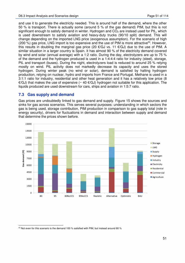
D6.3 Impact Analysis and Scenarios design Page 51 of 114
51
and use it to generate the electricity needed. This is around half of the demand, where the other 50 % is transport. There is actually some (around 5 % of the gas demand) PtM, but this is not significant enough to satisfy demand in winter. Hydrogen and CO2 are instead used for PtL, which is used downstream to satisfy aviation and heavy-duty trucks (90/10 split) demand. This will change depending on the imported LNG price (exogenous assumption). For the scenario of high (200 %) gas price, LNG import is too expensive and the use of PtM is more attractive53. However, this results in doubling the marginal gas price (20 €/GJ vs. 11 €/GJ) due to the use of PtM. A similar situation in a larger country is Spain. It has almost 90 % of the electricity demand covered by wind and solar (annual average) with a 1:2 ratio. During the day, electrolyzers are up to 75 % of the demand and the hydrogen produced is used in a 1:4:4:4 ratio for industry (steel), storage, PtL and transport (buses). During the night, electrolyzers load is reduced to around 25 % relying mostly on wind. PtL activity does not markedly decrease its capacity and uses the stored hydrogen. During winter peak (no wind or solar), demand is satisfied by halting hydrogen production, relying on nuclear, hydro and imports from France and Portugal. Methane is used in a 3:1:1 ratio for industry, residential and other heat generation and it has a relatively low price (8 €/GJ) that makes the use of expensive (~ 40 €/GJ) hydrogen not suitable for this application. The liquids produced are used downstream for cars, ships and aviation in 1:5:7 ratio.
7.3 Gas supply and demand
Gas prices are undoubtedly linked to gas demand and supply. Figure 15 shows the sources and sinks for gas across scenarios. This serves several purposes: understanding in which sectors the gas is being used, storage contribution, PtM production in comparison to gas supply total (role in energy security), drivers for fluctuations in demand and interaction between supply and demand that determine the prices shown before.
53 Not even for this scenario is the demand 100 % satisfied with PtM, but instead around 80 %

D6.3 Impact Analysis and Scenarios design Page 52 of 114
52
Figure 15. Gas supply (lower) and demand (upper) breakdown across main scenarios.
The range of flows varies between 3800 and 14000 PJ. To put these in perspective, gas demand for 2016 in EU28 was close to 18 EJ (~5000 TWh). Even in a BAU scenario, gas demand is not much different than a flexible 80 % CO2 reduction scenario. It only has a different distribution among sectors with the largest difference of LMG use for transport. As the system becomes more restricted, gas demand is progressively reduced. A commonality among scenarios is the low contribution from the residential sector, which shifts away from gas even for low CO2 target (see Appendix 12), giving its way to electricity as energy carrier and energy efficiency measures to reduce the final demand (which can reduce energy demand by 30-40 %). Only Spain and Italy retain 30-40 % of its current demand, where gas is used for cooking, while countries with a high fraction of gas for heating like Germany and the Netherlands make a drastic change away from gas. Similarly, the industry sector is a relative constant across scenarios. Its use for heat and steam production varies between 1800 and 3600 PJ depending on the scenario. The largest variants are the electricity and the commercial sector. Gas for electricity plays a larger role in the scenarios that have CO2 storage as possibility. However, it is also required that the biomass potential is at most at its reference value (~10 EJ/yr) and not higher. In such case (“Alternative” scenario), biomass displaces gas in electricity taking advantage of the negative emissions of biomass plus CCS and using this benefit in other sectors. This last effect is what in turn causes the fluctuations in the commercial sector. When biomass is used for electricity (and hydrogen) production, the negative emissions can balance the positive emissions in the commercial sector, which are more costly to reduce. Only when the scenario is more restrictive (either target or alternatives), the more expensive emissions from the commercial sector are reduced resulting in a lower gas demand. If CO2 storage is available, methane is used for hydrogen production (instead of the opposite). In terms of supply, the largest contribution is from Norway. It has the advantage of large reserves (350 EJ) and low production cost (1.2 €/GJ). In spite of having an upper annual production bound (of around 4400 PJ), it satisfies up to 80 % of the demand. This level of production is feasible considering its current production is around 4000 PJ. The largest fraction is attributed to the lower total gas demand. This is complemented by import by pipeline from outside the EU and LNG

D6.3 Impact Analysis and Scenarios design Page 53 of 114
53
import. Gas from the Netherlands has decreased by at least 70 % compared to current values to 100-700 PJ/year. Other sources include gas from UK, Germany, Romania and the upgrading of biogas with carbon capture. The role of PtM is limited in most of the scenarios and it only contributes significantly to energy independence in the “Optimistic” scenario. It provides up to 1.5 % of the gas demand in the “Alternative” scenario or even with 95 % CO2 reduction and no CO2 storage. In the “Realistic” scenario, it has 40 GW (280 PJ) of installed capacity (see Appendix 8) and satisfies close to 8 % of the gas demand. If the efficiency in marine transport is attractive enough to cause a shift in energy carrier to LMG, then PtM capacity increases to 122 GW (840 PJ) and 19 % of total demand. Naturally, the largest PtM contribution is when all the conditions that favor PtM are present. This implies the co-occurrence of 11 conditions away from the reference scenario (see Table 32 in Appendix 7). For this scenario, PtM capacity reaches 546 GW (4900 PJ) across EU28+ and providing 75 % of the gas demand. This “Optimistic” scenario has almost 6% higher annual costs compared to the “Realistic” scenario (see Figure 13), mainly because drivers that favor PtM (such as high gas price for import, higher cost for electricity grid expansion and low PtL performance) actually result in a higher cost to achieve the same CO2 target. The gas allocation among sectors is similar to the scenario with 80 % CO2 reduction and no CCS. Some changes are that there is no H2 production from methane when PtM is the source (since it would lead to inefficiency) and that LMG covers completely the marine transport and heavy-duty sectors. The single change that causes the largest positive change in PtM deployment is when the other options for CO2 sink are not available. In the scenario when there is no PtL (in addition to no CO2 storage), PtM total capacity is 482 GW (4400 PJ). A better PEM performance enabling cheaper hydrogen can lead to 263 GW of PtM capacity (vs. 122 GW). A high CO2 reduction target and absence of CO2 storage, even together, prove to be necessary, but not sufficient to make PtM attractive, with only 7 GW of PtM deployed in this scenario. The system drivers have a larger influence than the technology drivers. This means that even with low PtM Capex (< 100 €/kW) and highest efficiency for the technology, the deployment is zero if CO2 storage is still an alternative54. Three regulatory measures to promote PtM technology have been assessed within this study: (1) direct PtM capex subsidy, (2) indirect fossil gas tax, and (3) minimum target share of methane from PtM. With gas tax and minimum target share increasing the commodity price, they cause unwanted side effects such as a reduction of gas demand potentially motivating a fuel shift. The more effective instrument between tax on gas and PtM subsidy in terms of capacity installed is direct subsidy of the technology which leads to almost 6 times the deployment of a higher tax. A reason for this is that tax will increase gas price and will decrease the demand (through elasticity), while subsidy only has influence over the technology making it directly more attractive. This is in agreement with previous studies that identify that “SNG from PtM processes is not competitive with natural gas or even biomethane [from fermentation processes]” and different simultaneous drivers are needed [147]. However, both instruments do not guarantee a certain minimum target share of methane from PtM as instrument (3) does. Setting a minimum target share that is the same for all European countries seems not advisable as it does not consider nationally differing hydrogen demand and supply structures that make PtM unequally attractive across European countries. To put these figures in perspective, estimates for Germany are 7.5 GW [139], 6-12 GW [31], 28 GW [171], 1-59 GW [172], 48-87 GW [46] and even 89-134 GW [57]. For Ireland, 0.5 GW has been explored [21], 5 GW in UK [173], 7-13 GW in Spain with 27 % VRE [174], Finland had 25 GW for a 100 % RES system [58]. On the global scale, PtM had over 2300 GW [27], which even considering a small fraction of this being deployed in EU28+ is still far above the results for most unrestricted scenarios in this study. Some differences of the present study with respect to the
54 Scenario“80CostEff”, which means 80 % CO2 reduction, low PtM Capex and high efficiency testing if the positive technology drivers outweigh the negative system drivers

D6.3 Impact Analysis and Scenarios design Page 54 of 114
54
previous references are: system boundaries, most of these studies [21,27,31,57,139,173] focus only on the power system. This leaves options like Power to Liquid and hydrogen for transport (the two dominant flexibility options for this study) out of scope, which might overestimate both electricity storage and PtM role. Other approaches (e.g. [174]) only estimate the power surplus and its potential use for PtM. Some of the studies focus on the operational aspect (e.g. hourly electricity price and operating hours) rather than the investment component and only do PtM capacity as sensitivity, which might lead to sub-optimal combinations, whereas in the current study the capacity is an output of the calculation. Finally, some studies (e.g. [21,175]) have gas demand as an exogenous variable, whereas in this study it is the result of the competition among technologies (endogenous). Today, almost 20 % of the gas is used in the residential sector for heating and gas constitutes 40 % of the fuel mix to satisfy the heating and cooling services across EU [135]. This represents one of the main reasons to support PtM, where it is foreseen that to continue satisfying the heat demand, a lower carbon route has to be found for the gas. Nevertheless, across the range of scenarios evaluated, remaining heating demand after considering energy efficiency, is mainly satisfied with electricity (a range between 70-85 %), complemented (5 %) by biomass, solar (0-15 %) and district heat (10 %). Gas role in residential heating is reduced to district heating, where its application is mainly through central CHP with carbon capture (see Appendix 12). Since LMG constitutes a large part of gas demand, drivers that promote LMG have a positive impact on gas demand. The order of magnitude for the energy consumed in heavy-duty, marine transport and buses (sectors where LMG can be used) is 5000, 2000 and 500 PJ respectively. The fuel choice for marine transport is directly dependent on commodity price and efficiency (leading to €/km). Consequently, when the efficiency is high enough, this sector is satisfied with LMG rather than diesel/HFO55. Buses are fueled with hydrogen in most scenarios, except if the electric option is possible or by diesel in BAU. Heavy duty is both the largest demand and the one with the largest changes across scenarios (see Appendix 13 for the fuel mix for the different transport modes across the main scenarios). LMG is used either if the CO2 target is low (80 %) or if CCS is available (which leads to negative emissions when combined with biomass and positive emissions can be afforded in transport). In scenarios with a high biomass potential, where CO2 could be used for PtM, CO2 is used instead for PtL to produce diesel. The lower efficiency of the PtL process (78 % for Fischer Tropsch [164], while it is 85 % for PtM, see Table 5) is compensated by the higher efficiency and lower cost of diesel trucks downstream (7.5 vs. 8.9 MJ/km and almost 20k€ cheaper by 2050 [164]). Even in the scenarios where LMG is used across these sectors, the LMG is sourced in imports for the scenarios where LMG is used in heavy-duty trucks complemented by large scale liquefaction of imported gas. The value chain of liquefaction of PtM product is not selected. Therefore, the same conditions that favor the use of LMG for heavy-duty trucks are the ones that do not favor PtM (low CO2 target and use of CCS). This proves that the additional cost for hydrogen distribution and refueling (4.6-6 €/kgH2) plus the higher (+35%) cost of the end vehicle itself is still smaller than the extra cost caused by efficiency losses in PtM (10-15%), liquefaction (6-8%), end use (energy consumption in an LMG truck is 45% higher than one with fuel cell [164]). Considering as well that the PtM route involves extra Capex for both steps (PtM and liquefaction), while the saving is the distribution infrastructure. This does not even consider the extra costs for refueling stations that would be needed for LMG. Another factor is that PtM use in these sectors will incur in CO2 emissions at the point of use. This requires another system to be in place to track the source of the CO2 emitted and legal frameworks to ensure compliance. In contrast, hydrogen has zero tailpipe emissions and CO2 emissions (if any) are centralized. These two reasons make hydrogen more attractive for these two sectors (heavy-duty and buses) as the scenario becomes more restricted.
55 Diesel from Power-to-Liquid/Biomass-to-Liquid when LMG efficiency is low and HFO only for BAU scenario

D6.3 Impact Analysis and Scenarios design Page 55 of 114
55
From the above, a key parameter is the efficiency considered for LMG in ships. However, diesel engines are also expected to improve their performance and this could actually represent up to a third of the CO2 mitigation in this sector [165]. If this is considered, efficiency for both fuels would be comparable and fuel choice is left to other factors. LMG would have the disadvantage of the need to develop new bunkering infrastructure. Doing this in the major 160 ports around the world, would cost around 11 bln$ [165], excluding all the upstream costs. LNG can have up to 200 % of the life cycle emissions compared to conventional NG [176], which would make it more challenging until PtM is large enough to satisfy all demand. The methane losses in the parts of the system that would remain with PtM (e.g. storage, long distance transport by pipelines, distribution to costumers) can be 1.4-3.6 % of the gas produced [177]. This can increase the GHG life cycle emissions by 25-50 %. LMG also implies a more complex on-storage system for the vessels, additional training, less space for loads (since the storage is larger), additional investment for ship adaptation and new safety regulations [165]. For these reasons, the “Realistic” scenario in this study does not consider LMG as dominant fuel for navigation.
7.4 Seasonal component of PtM
VRE represents up to 70 % of the electricity mix. This introduces a strong seasonal and daily component in production. Electrolyzers (mostly for the scenarios without CO2 storage) represent up to 40 % of the electricity demand and even larger fractions for specific countries or time slices. Their share is large enough to influence electricity prices by manipulating demand. There is almost (< 1 %) no hydrogen production during the winter peak (when there is no wind and solar contribution) and for countries dominated by solar, a similar behavior is observed during night. Production during summer peak can be up to 3-4 times higher than peak for the other two seasons. This produces a flattening effect of the electricity prices. Prices in summer can be 25 % lower than in spring or fall, while prices in winter can be up to 80 % higher (this also includes a capacity adequacy component to ensure there is enough capacity to satisfy the winter peak). Hydrogen prices in turn are attenuated by both the use of hydrogen storage (in tanks for daily fluctuations) and relatively flexible demand (when it is used for PtX). Consequently, hydrogen prices only fluctuate up to +/- 10 % across time slices. This flexible operation causes the electrolyzers to be operating only close to 50% of the time. In spite of the higher Capex contribution caused for this, it still results an attractive option. This lower difference in daily prices reduces the incentive for price arbitrage through storage, which will only become smaller as the storage capacity increases [178]. PtM makes use of these small price differences across seasons and there is a seasonal pattern observed for PtM activity (see Figure 16 and Appendix 8). The seasonal storage fraction (primary Y-axis in Figure 16) indicates the fraction of PtM gas that is stored each season compared to the total amount of PtM product routed to storage. The secondary Y-axis on Figure 16. Fraction of PtM production stored in each season across all scenarios.
indicates the fraction of PtM routed to storage for every scenario compared to the total PtM energy produced. Stored fraction during summer can be up to double the fraction stored in spring or fall, while the fraction stored in winter can be around half of these, only sustained by countries with a significant wind contribution. This effect is more pronounced (see Appendix 8) as the scenario becomes more restricted. Similarly, around 70-90 % of the PtM product is routed through storage and then mixed with the rest of the gas, although it can be used in some cases within the same season. The main driver for seasonal storage is to satisfy demand when there is a low contribution from VRE in a system where other dispatchable RES technologies capacity is low. This application is investigated using the winter peak time slice. The intermediate scenario (only wind) presents itself over every night time slice. The technologies that provide flexibility when there is no VRE are
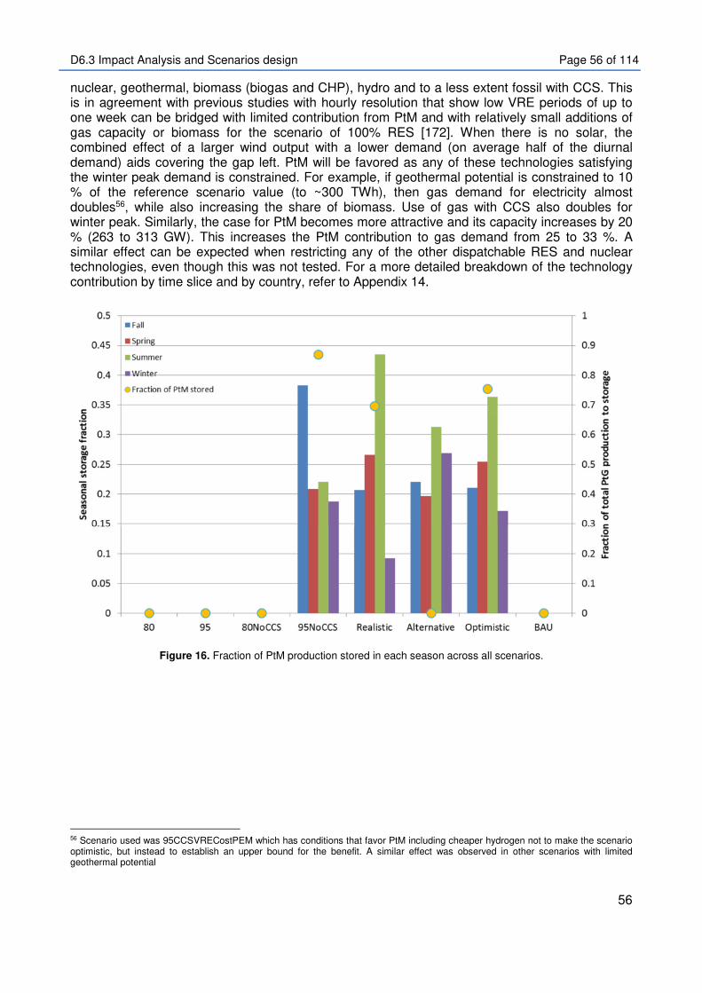
D6.3 Impact Analysis and Scenarios design Page 56 of 114
56
nuclear, geothermal, biomass (biogas and CHP), hydro and to a less extent fossil with CCS. This is in agreement with previous studies with hourly resolution that show low VRE periods of up to one week can be bridged with limited contribution from PtM and with relatively small additions of gas capacity or biomass for the scenario of 100% RES [172]. When there is no solar, the combined effect of a larger wind output with a lower demand (on average half of the diurnal demand) aids covering the gap left. PtM will be favored as any of these technologies satisfying the winter peak demand is constrained. For example, if geothermal potential is constrained to 10 % of the reference scenario value (to ~300 TWh), then gas demand for electricity almost doubles56, while also increasing the share of biomass. Use of gas with CCS also doubles for winter peak. Similarly, the case for PtM becomes more attractive and its capacity increases by 20 % (263 to 313 GW). This increases the PtM contribution to gas demand from 25 to 33 %. A similar effect can be expected when restricting any of the other dispatchable RES and nuclear technologies, even though this was not tested. For a more detailed breakdown of the technology contribution by time slice and by country, refer to Appendix 14.
Figure 16. Fraction of PtM production stored in each season across all scenarios.
56 Scenario used was 95CCSVRECostPEM which has conditions that favor PtM including cheaper hydrogen not to make the scenario optimistic, but instead to establish an upper bound for the benefit. A similar effect was observed in other scenarios with limited geothermal potential

D6.3 Impact Analysis and Scenarios design Page 57 of 114
57
7.5 CO2 sources and sinks
PtM should use CO2 from biogenic sources for the following reasons: (1) The CO2 will ultimately be emitted and if the CO2 is sourced from fossil it will cause a net positive increase of CO2 in the atmosphere; (2) if CO2 comes from an ETS (Emissions Trading Scheme) sector (e.g. power) and ultimately ends up in a sector not covered by ETS (e.g. transport), it could lead to an emissions reduction for ETS, while in reality not leading to a reduction of CO2 emissions for the entire system; (3) it could prolong the use of fossil fuels in the energy system. The sources and final sinks of CO2 across the main scenarios are shown in Figure 17. Note that for the second reason, the model does contain the ETS and ESR (Effort Sharing Regulation covering non-ETS sectors) policies until 2030 (43 and 30 % reduction respectively compared to 2005 levels). For 2050, the CO2 target is for the entire system regardless of sectors.
Figure 17. CO2 sources and sinks across main scenarios. For the scenarios where CO2 underground storage is possible, it is the preferred sink for CO2. Sources are varied across power (BECCS, fossil CHP and gas), H2 production (with biomass and most of “Others” category) and industry. With the reference biomass potential, biomass provides around 25 % of the CO2 that ultimately ends up underground (three main routes: combined cycle for power, H2 production and BtL). With the highest biomass potential (e.g. “Alternative” scenario) biomass supplies close to 80 % of the CO2 stored. These emissions allow for (the most expensive) positive emissions elsewhere in the system. Only when CO2 storage is not possible, CO2 use arises. This techno-economic approach supports the environmental conclusion that when CO2 storage is an alternative, that is the best sink for the CO2 when compared to methane [9,10,179]. Furthermore, when there is CO2 use, the preferential sink is Power-to-Liquid. In the “Realistic” scenario PtL is almost 25 times larger (in terms of CO2 consumption) than PtM. A key sector that promotes this trend is aviation. The total demand for EU28+ is close to 4000 PJ, which translates to almost 0.3 Gton of CO2 if all that demand were to be satisfied by PtL. Not all of it is satisfied with PtL and the ratio is about 4:1 PtL/BtL. It even has fossil-derived fuels for 80 and 95 % CO2 reduction scenarios. Another smaller driver is the use of diesel in private cars (500 PJ). Electricity dominates private transport and the extra cost of the electricity network is outweighed

D6.3 Impact Analysis and Scenarios design Page 58 of 114
58
by the higher pathway efficiency. To avoid an overly optimistic reliance on electric vehicles, their share is limited to 80 % (assumption by authors). Part of the 20 % remaining is covered by diesel vehicles (most efficient ones [180]), biofuels and hydrogen. More detail on the dynamics of PtL is part of a separate study focused on H2 and PtL [181] (in preparation). When there is neither PtL nor CO2 storage, PtM is used, but CO2 flow is reduced by 30 %. CO2 use for PtM can be up to one third of the total CO2 captured when PtM has a higher efficiency and almost 75 % for the “Optimistic” scenario. A tax on gas has limited effect on CO2 use, as its main effect is to reduce natural gas consumption rather than significantly increase PtM. The largest CO2 consumption is for the “Optimistic” scenario. Close to 270 Mton/yr are used for PtM, representing close to 5000 PJ of methane, which translates to 6000 PJ of H2 input and almost 2000 TWh of electricity input required to satisfy such demand. This is more than half the current annual generation for EU (at 3200 TWh) only because of the additional constraints introduced (see Appendix 7 for constraints of “Optimistic” scenario). For this scenario, 70 % of the CO2 used for PtM comes from biomass (BtL), 18 % comes from industry and even a 10 % from combined heat and power with fossil (see Appendix 8 for a better visualization). Two alternatives are identified. In one case, specific BtL plants could be co-located with wind farm/commercial solar plants and there would be a one-to-one match of CO2 sources or sinks. In another one, there is a CO2 network and all the producers and consumers are connected to the network without the possibility of allocating a consumer to a specific producer since they are all interacting through the grid. The model uses the second approach, coupled with the representation of one country per node, it is not possible to allocate specific BtL sources for PtM. However, it is optimistic to assume that all the CO2 produced by BtL can be used by PtM, because it would imply that all the sites would have either wind or solar surplus, a nearby (suitable) biomass source, limited electricity grid capacity and enough gas grid capacity (otherwise PtM loses its claimed advantage of using existing facilities). This representation does not necessarily imply that full nationwide CO2 networks need to be developed. Instead, main sources and sinks could be connected through critical pipeline corridors, perhaps even partly using former natural gas infrastructure. A CO2 source that has a limited contribution across scenarios and that has been identified as preferential for PtM is biogas production. CO2 capture on biogas occurred only when CO2 storage was possible. Raw biogas is directly used for electricity, heat and steam generation through CHP for industrial use [181] (in preparation). This even assumes a cost penalty in Capex due to adaptation of equipment to use the lower heating value gas. Throughout the scenarios studied, biogas was used around 75-90 % for steam and heat generation in industrial processes in scenarios with CO2 storage and mainly (65 %) for electricity generation when CO2 storage was absent. Additionally, studies [94] suggest that upgrading with amines (standard process) has lower GHG emissions and other LCA indicators (human health, ecosystem and resources) than upgrading with PtM. Only for scenarios with a high biomass potential, PtM for biogas upgrading appeared as potential option. A high biomass potential, promotes the less efficient gas use in residential and commercial sector (due to the negative CO2 emissions), which increases gas prices (in some countries even doubles), while at the same time causing a saturation effect in the biogas (industrial) users that produces a decrease (20-70 %) of the biogas price. A cheaper feed and more expensive methane increase PtM attractiveness, but even then it only supplies up to 0.3 % of the gas demand.
7.6 Drivers and barriers for PtM
An advantage of the parametric scenario analysis done is that the effect for individual changes can be assessed. This allows determining (1) the extent to which each one affects the entire system (e.g. energy balances and cost), but also the effect on PtM deployment and (2) which ones have a positive effect on deployment and which ones might limit its contribution. This is

D6.3 Impact Analysis and Scenarios design Page 59 of 114
59
important since on one hand the evolution of the energy system is uncertain and it could go either direction (one where PtM is dominant or one where PtM is limited) and on the other hand some of these parameters (e.g. PtM Capex) can be influenced by further research and demonstration. Based on the 120 scenarios run, some trends were observed. Figure 18 shows the main parameters that have influence on PtM. The effect was quantified by looking at capacity deployed and energy delivered for various scenarios. On the right side (of Figure 18) are the extremes that were tested in this study and that favor PtM, while the left side reflects the extremes that are least favorable for PtM. Table 17 shows a relative ranking of the parameters with the largest weight assigned to the ones with the largest effect (on PtM deployment). This is not done on a specific formula, but done on a qualitative basis based on the output from the scenarios. For some further understanding, refer to the set of scenarios run (Table 32) and PtM capacity deployed across scenarios (Figure 36).
Figure 18. Main parameters with influence on PtM deployment. Green means it favors PtM, while red means it hinders
its deployment. The intermediate values in Figure 18 (with shaded area) represent values where a change in trend (from hindering to favoring) was observed. The reason to make it shaded is because such value is not unique and highly depends on the rest of the assumptions (and not based on a single parameter). Thus, for example, 60% of VRE penetration is established as tipping point since there were no scenarios observed with lower penetration where PtM was deployed. However, there could be cases, where gas is so expensive or the technology is subsidized that could make a system with 50% penetration attractive for PtM. In the case of efficiency, anything above the reference efficiency (see Table 5) would be a positive effect for PtM since it creates an additional revenue stream. When comparing Figure 18 with Table 17, some of the items were left out due to: (1) Ranking of 1 or 2; (2) a single value cannot be captured in Figure 18 (e.g. PEM performance which is a set of values on Table 7 and Table 8 or PtL performance which are the parameters on Table 25); (3) as has been discussed in Section 7.4 if there are any additional

D6.3 Impact Analysis and Scenarios design Page 60 of 114
60
limitations considered for power generation (e.g. limited coal, nuclear, geothermal, hydro), the effect will be positive for PtM deployment. PtM was not deployed for scenarios with 80% CO2 reduction (914 Mton CO2/year) regardless of the other parameters varied. For this reason, most of the scenarios focused on 95% CO2 reduction (228 Mton CO2/year), while the shaded area (around 450 Mton/year), there could be some deployment depending on the rest of assumptions. With respect to CO2 storage, its capacity would have to be very limited for PtM to be attractive, since it is cheaper and puts away permanently the molecule. Only when it is not enough to store the CO2 for the entire lifetime or for all the emissions, the CO2 is used (see Section 7.5). For the Capex, no specific tipping point was identified, but the concrete observation is that more restrictions were needed to promote deployment with the high side of the range explored. For LMG used in ships, the most important parameter is not the absolute efficiency (12-25 gCO2/(t*nm)), but the relative difference with diesel/HFO engines and potential increase in demand (see Sections 5.5 and 7.3). For biomass potential, there is a mixed effect. For higher potentials there is more CO2 that has near zero footprint that can be used for PtM, while at the same time, the higher potential also decreases the marginal CO2 price and reduces the incentive for PtM. The effect on CO2 price is stronger for PtM since that affects directly the attractiveness of the technology. Therefore, lower potentials will favor PtM (since these limit the most system flexibility).
Table 17. Relative ranking of parameters having influence on PtM deployment.
Parameter Category57 Weight Comment
CO2 reduction target System 5 PtM plays a limited role in 80% CO2 reduction target scenarios even when technology drivers are optimistic
CO2 storage System 5 PtM is attractive only when CO2 storage is not possible or very limited (since the CO2 is put away permanently and at a lower cost)
VRE penetration System 5 If there is not enough surplus, there is less need for PtX
PtM Capex Technology 4 Lower Capex can increase PtM capacity by 4-5 times
PtM Efficiency Technology 4 It provides an additional revenue stream (heat that improves economic attractiveness
PtM subsidy Technology 4 Highly effective, but this could result in inefficiency (hydrogen production from PtM) just to take advantage of the subsidy
PtL performance Technology 4 Can double with "Conservative" PtL performance or halved with "Optimistic" PtL performance (see Table 25)
PEM performance Technology 3 Cheap (<= 3 €/kg) hydrogen is needed for PtG, but if the PEM performance is higher other sectors might take advantage of it
Geothermal potential System 3 The more restricted other power technologies are, the more attractive gas will be
Nuclear policy System 3 The more restricted other power technologies are, the more attractive gas will be
57 System means it applies to the entire energy system (e.g. CO2 storage) and driven by policies beyond PtM, while “Technology” refers to a more specific scope of a technology that could be de-risked by R&D

D6.3 Impact Analysis and Scenarios design Page 61 of 114
61
LNG efficiency in ships
Technology 3 More important than the absolute value is the difference compared to other energy carriers. Even in an optimistic scenario, additional demand is up to 2 EJ corresponding to 10% of current (2016) gas demand
Biomass potential System 3 More biomass provides more CO2 for PtM, but also reduces CO2 price making PtM less attractive
Electric option for buses and trucks
Technology 2 Investment is lower and efficiency is higher than LNG trucks
Electricity network cost
System 2 Effect can actually be negative: (1) Reduces attractiveness of centralized gas power plants; (2) Makes H2 more attractive (since it is the preferred energy carrier after electricity)
No coal policy System 2 Coal plays a limited role in power and this affects hydrogen more (use in steel)
Gas price System 2 Shifts all prices upwards and decreases demand rather than promoting PtM significantly
Gas tax System 1 It affects mostly gas consumption rather than PtM directly
PtM discount rate Technology 1 Driven by system need rather than economic opportunity
DSM System 1 Most flexibility provided by hydrogen
It was observed that system drivers have a larger influence than technology drivers. A scenario with 80% CO2 and CO2 storage available (both negative drivers), but with low PtM Capex and high efficiency (both positive technology drivers) had very limited (< 1 GW) deployment. Based on the results, the system drivers with the largest influence are CO2 target, CO2 storage and VRE penetration. The “Optimistic” scenario assumes the co-occurrence of 11 parameters that favor PtM (see Table 32), but the ranking of parameters in Table 17 allows understanding the influence of the different parameters and construct new scenarios as needed for other tasks.
D6.3 Impact Analysis and Scenarios design Page 62 of 114
62
8 Conclusions
In this study, drivers and potential for power-to-methane (PtM) in various scenarios were investigated. The results show, among others, for each scenario the installed PtM capacity, effect over energy balances and the total costs for a future energy system. For 21 out of 55 low carbon scenarios analyzed in this study, PtM capacity lies in the range of 40 to 200 GW. From the CO2 perspective, the preferred sink is underground storage. Only when storage is restricted, CO2 use for fuels is possible. In such case, CO2 captured reduces drastically from 1.5-1.75 to 0.2-0.35 GtonCO2/yr. From the energy carrier perspective, electricity is preferred. Electricity satisfies up to 50 % of the final demand and production doubles compared to current values (6200 vs. 3200 TWh) with a target of 95 % CO2 and can reach up to 11000 TWh for more constrained scenarios. From an electricity flexibility perspective, hydrogen production plays a significant role. Electrolysis is the preferred route when there is no CO2 storage and its demand can be up to 40 % of the electricity produced (on average for the entire EU28+). It can drastically change the demand curve to partially follow generation and decrease price fluctuations. However, the flexibility does not extend to methane, but propagates to PtL and other hydrogen applications (dynamics for H2 and PtL are part of a separate study in preparation [62]). The main driver for PtL preference over PtM is the aviation demand. This is between 4 to 5 EJ/year that only have PtL and BtL as options. In spite of this, annual costs for the electricity network are 105-140 bln€/yr. Gas demand, decreases by 30-80 % to levels between 3800 and 14000 PJ (today around 20 EJ). For scenarios without CO2 storage (which is a necessary condition to have PtM), gas is displaced by RES in power, displaced by electricity in heating and left mostly for industrial heat and steam generation. From an energy independence perspective, PtM can reduce gas imports. In the “Realistic” scenario, it satisfies close to 8 % of the gas demand, while this increases to almost 75 % for the “Optimistic” scenario. The rest of the gas demand continues to be satisfied with gas from Norway, import by pipeline (Russia) and LNG. From a cost perspective, PtM effect on marginal CO2 price is 2 % when the technology has a high efficiency. Annual costs for PtM range from 2.5 bln€/yr for the “Realistic” scenario and up to 10 bln€/yr for the “Optimistic” scenario, with a split close to 70/30 in Capex/Opex. This represents a fraction of 0.05-0.25 % of the total annual system costs and 0.45 to 5.7% of the gas supply costs (which are in the order of 200 to 300 bln€/yr). Energy security improves instead as an effect of reducing total CO2 emissions. This promotes electrification and BtL/PtL, which combined allow reducing the import bill from 400 bln€/yr for BAU, to 250 bln€/yr for 80% CO2 reduction and further to 190 bln€/yr with 95% CO2 reduction. To put these annual costs in perspective, GDP for EU28 was 15.3 trillion€ for 2017. LMG has a large contribution to the overall gas demand (up to 50 %). LMG is used mainly for marine transport and heavy-duty trucks. The energy demand for these sectors is expected to be around 2000 and 5000 PJ respectively by 2050. If the efficiency of gas-fired propulsion systems for ships is high enough (12 gCO2/(ton*nm) was used as optimistic value), then marine transport is satisfied with this energy carrier promoting PtM. For heavy-duty, LMG is used either when the CO2 target is relatively low (80 % CO2 reduction) or if CCS is available. This is because LMG in heavy-duty could be part of the 20 % of emissions remaining or be compensated by negative emissions elsewhere in the system (when CCS is combined with biomass). Even when used for these sectors, LNG is imported complemented by domestic large scale liquefaction. This is naturally dependent on gas (LNG) price and with increases in gas price, the fraction of domestic liquefaction increases. The drivers for use of LMG in heavy-duty trucks are the ones that hinder PtM deployment (namely CO2 storage and low CO2 target). PtM deployment was 40 GW (280 PJ of methane produced) across EU28+ for the “Realistic” scenario. This implies 95 % CO2 reduction, no CO2 storage, low PtM Capex (75 €/kW) and a low efficiency for LMG use in ships (25 gCO2/(ton*nm)). A high efficiency for ships increases gas demand and PtM capacity to 122 GW (840 PJ). A high VRE is a necessary, but not sufficient
D6.3 Impact Analysis and Scenarios design Page 63 of 114
63
condition for PtM. Countries with up to 95 % electricity from VRE did not have PtM. Flexibility for these countries was mostly provided by electrolysis, but it did not extend to methane. Similarly, CO2 storage absence and high CO2 target are necessary, but not sufficient. A scenario with these two conditions, but still with a high (750 €/kW) PtM Capex, only had 7 GW deployed across EU28+. The “Optimistic” scenario, which had the simultaneous variation of 11 parameters away from the reference scenario, had the largest PtM capacity with 546 GW (4900 PJ), supplying almost 75 % of the gas demand. The two largest drivers are cheaper hydrogen (through better PEM performance) and a higher PtM efficiency (through heat recovery). The former also favors PtL, although the relative change in PtM is larger, while the latter requires a nearby consumer for the heat with a high willingness to pay. Technology subsidy of 3 €/GJ in 2050 for PtM (compared to gas prices between 8-20 €/GJ) increases deployment by around a third of the capacity (from 122 GW to 165 GW). This is a more effective measure to deploy the technology since taxing the fossil alternative (i.e. natural gas) leads to a larger gas demand reduction, but not necessarily to more PtM deployment (122 to 128 GW). The assessed minimum target share for methane from PtM seems little advisable despite being the most powerful instrument of the three investigated regulatory measures since it implies the highest probability of unwanted side effects such as increase of gas price and hence decrease of gas demand and fuel shift. PtM does exhibit a seasonal component in its production. Production in summer peak can be twice the production during spring or fall, while production in winter can be around half of it. 70-80 % of PtM production goes through (existing) underground storage. However, most of the flexibility for VRE integration is provided by electrolyzers and variable hydrogen production rather than PtM, while periods of low VRE generation are bridged by a combination of hydro, nuclear, biomass (biogas and CHP) and geothermal. If any of these options is constrained further, the outlook for PtM improves. When geothermal potential is limited to 300 TWh in EU28+ (to put this in perspective, generation in 2015 was around 15 TWh, while the full potential is 3000 TWh [72]), PtM capacity increases by 20 %. CO2 sources for PtM are mostly biogenic. Nevertheless, for the “Optimistic” scenario, even though 70 % of the CO2 originates from biomass (BtL), there is also 18 % from industry and 10 % from combined heat and power with fossil fuels. No individual sources and sinks are paired in the model and instead there is a single commodity (CO2 for use) equivalent to a network, where the users withdraw their share. In case a similar scheme arises in reality, ensuring that PtM operates only with biogenic sources might become more cumbersome. The results are bound to model limitations that should be the scope of further studies. One is the spatial resolution. The model considers one country per node and does not include the location of demand centers, high VRE potential locations, routing of electricity and natural gas grid or location for CO2 sources. Constraints arising from local consideration of these parameters might change the conclusions reached in this study. A detailed representation of the networks within the countries will lead to identifying local spots where the grid cannot accommodate the entire VRE production leading to higher local surplus. A higher spatial resolution most likely also compromises either spatial or sectorial coverage, where this model prevails. Positive effects from system stabilizing behavior and regional ancillary services of distributed technologies such as kW- and MW-scale gas-CHP were not investigated and could lead to local business cases for PtM. The other main limitation is temporal resolution. The model represents a year with 12-24 time slices. Hourly resolution for electricity would allow having a better estimate of the surplus, storage role and adjustments in generation. On even a shorter time scale, balancing and grid services could provide additional revenue streams for electrolysis making the process more attractive. However, this might favor hydrogen rather than methane. Finally, this study covers the techno-economic aspect. This should be complemented with the environmental and societal perspective to be able to conclude about the effect and outlook of the technology. With large infrastructure projects facing social acceptance issues, distributed technologies have a steadily growing advantage.

D6.3 Impact Analysis and Scenarios design Page 64 of 114
64
9 References
[1] Engineering AS of D for R and. Technology Readiness Assessment (TRA) Guidance. Dep Def 2011.
[2] Commission E. HORIZON 2020 - WORK PROGRAMME 2016 – 2017. Section 20 . General Annexes (European Commission Decision C(2017)2468). Work Program 2016 – 2017 2017:20.
[3] Mankins J. Technology Readiness Levels. Off Sp Access Technol 1995:4.
[4] Fendt S, Buttler A, Gaderer M, Spliethoff H. Comparison of synthetic natural gas production pathways for the storage of renewable energy. Wiley Interdiscip Rev Energy Environ 2016;5:327–50. doi:10.1002/wene.189.
[5] Grond L, Holstein J. Power-to-gas: Climbing the technology readiness ladder. Gas Energy 2014:20–5.
[6] de Bucy J, Lacroix O, Jammes L. The Potential of Power to Gas. Paris: 2016.
[7] Vandewalle J, Bruninx K, D’Haeseleer W. Effects of large-scale power to gas conversion on the power, gas and carbon sectors and their interactions. Energy Convers Manag 2015;94:28–39. doi:10.1016/j.enconman.2015.01.038.
[8] Schill WP. Residual load, renewable surplus generation and storage requirements in Germany. Energy Policy 2014;73:65–79. doi:10.1016/j.enpol.2014.05.032.
[9] Reiter G, Lindorfer J. Global warming potential of hydrogen and methane production from renewable electricity via power-to-gas technology. Int J Life Cycle Assess 2015:477–89. doi:10.1007/s11367-015-0848-0.
[10] Sternberg A, Bardow A. Life Cycle Assessment of Power-to-Gas: Syngas vs Methane. ACS Sustain Chem Eng 2016;4:4156–65. doi:10.1021/acssuschemeng.6b00644.
[11] Meylan FD, Piguet F-P, Erkman S. Power-to-gas through CO2 methanation: Assessment of the carbon balance regarding EU directives. J Energy Storage 2017;11:16–24. doi:10.1016/j.est.2016.12.005.
[12] Zhang X, Bauer C, Mutel CL, Volkart K. Life Cycle Assessment of Power-to-Gas: Approaches, system variations and their environmental implications. Appl Energy 2017;190:326–38. doi:10.1016/j.apenergy.2016.12.098.
[13] Simoes S, Nijs W, Ruiz P, Sgobbi A, Radu D, Bolat P, et al. The JRC-EU-TIMES model. Assessing the long-term role of the SET Plan Energy technologies. 2013. doi:10.2790/97596.
[14] Simoes S, Nijs W, Ruiz P, Sgobbi A, Thiel C. Comparing policy routes for low-carbon power technology deployment in EU – an energy system analysis. Energy Policy 2017;101:353–65. doi:10.1016/j.enpol.2016.10.006.
[15] Nijs W, Simoes S, Ruiz P, Sgobbi A, Thiel C. Assessing the role of electricity storage in EU28 until 2050. Int Conf Eur Energy Mark EEM 2014. doi:10.1109/EEM.2014.6861273.
[16] Sgobbi A, Nijs W, De Miglio R, Chiodi A, Gargiulo M, Thiel C. How far away is hydrogen? Its role in the medium and long-term decarbonisation of the European energy system. Int J

D6.3 Impact Analysis and Scenarios design Page 65 of 114
65
Hydrogen Energy 2016;41:19–35. doi:10.1016/j.ijhydene.2015.09.004.
[17] Simoes S, Zeyringer M, Mayr D, Huld T, Nijs W, Schmidt J. Impact of different levels of geographical disaggregation of wind and PV electricity generation in large energy system models: A case study for Austria. Renew Energy 2017;105:183–98. doi:10.1016/j.renene.2016.12.020.
[18] Nijs W, Simoes S, Sgobbi A, Ruiz-Castello P, Thiel C, Giannakidis G, et al. Improved Representation of the European Power Grid in Long Term Energy System Models: Case Study of JRC-EU-TIMES. Lect Notes Energy 2015;30:201–22. doi:10.1007/978-3-319-16540-0_12.
[19] Thiel C, Nijs W, Schmidt J, Zyl A Van, Schmid E. The impact of the EU car CO 2 regulation on the energy system and the role of electro-mobility to achieve transport decarbonisation. Energy Policy 2016;96:153–66. doi:10.1016/j.enpol.2016.05.043.
[20] Blanco H, Faaij A. A review at the role of storage in energy systems with a focus on Power to Gas and long-term storage. Renew Sustain Energy Rev 2018;81:1049–86. doi:10.1016/j.rser.2017.07.062.
[21] Ahern EP, Deane P, Persson T, Gallachoir BO, Murphy J. A perspective on the potential role of biogas in smart energy grids. Renew Energy 2015;78:648–56. doi:10.1016/j.renene.2015.01.048.
[22] Qadrdan M, Abeysekera M, Chaudry M, Wu J, Jenkins N. Role of power-to-gas in an integrated gas and electricity system in Great Britain. Int J Hydrogen Energy 2015;40:5763–75. doi:10.1016/j.ijhydene.2015.03.004.
[23] Breyer C. Economics of Hybrid Photovoltaic Power Plants. University of Kassel, 2012.
[24] Klumpp F. Potential for large scale energy storage technologies - Comparison and ranking including an outlook to 2030. Energy Procedia 2015;73:124–35. doi:10.1016/j.egypro.2015.07.659.
[25] Parra D, Patel M. Techno-economic implications of the electrolyser technology and size for power-to-gas systems. Int J Hydrogen Energy 2016;41:3478–761. doi:http://dx.doi.org/10.1016/j.ijhydene.2015.12.160.
[26] Belderbos A, Delarue E, D’haeseleer W. Possible role of Power-to-Gas in future energy systems. Leuven, Belgium: 2015. doi:10.1109/EEM.2015.7216744.
[27] Pleßmann G, Erdmann M, Hlusiak M, Breyer C. Global energy storage demand for a 100% renewable electricity supply. Energy Procedia 2014;46:22–31. doi:10.1016/j.egypro.2014.01.154.
[28] Moeller C, Meiss J, Mueller B, Hlusiak M, Breyer C, Kastner M, et al. Transforming the electricity generation of the Berlin e Brandenburg region , Germany. Renew Energy 2014;72:39–50. doi:10.1016/j.renene.2014.06.042.
[29] Kötter E, Schneider L, Sehnke F, Ohnmeiss K, Schröer R. Sensitivities of power-to-gas within an optimised energy system. Energy Procedia 2015;73:190–9. doi:10.1016/j.egypro.2015.07.670.
[30] Clegg S, Mancarella P. Integrated Modeling and Assessment of the Operational Impact of Power-to-Gas (P2G) on Electrical and Gas Transmission Networks. IEEE Trans Sustain

D6.3 Impact Analysis and Scenarios design Page 66 of 114
66
Energy 2015;6:1234–44. doi:10.1109/TSTE.2015.2424885.
[31] Jentsch M, Trost T, Sterner M. Optimal use of Power-to-Gas energy storage systems in an 85% renewable energy scenario. Energy Procedia 2014;46:254–61. doi:10.1016/j.egypro.2014.01.180.
[32] Daniëls B, Seebregts A, Joode J, Smekens K, Van Stralen J, Dalla Longa F, et al. Exploring the role for power-to-gas in the future Dutch energy system. 2014.
[33] Breyer C, Gulagi A, Bogdanov D. South-East Asia and the Pacific Rim Super Grid for 100 % Renewable Energy power supply South-East Asia and the Pacific Rim Super Grid for 100 % RE power supply Christian Breyer , Ashish Gulagi and Dmitrii Bogdanov 2015. doi:10.13140/RG.2.1.1798.4729.
[34] Breyer C, Bogdanov D, Komoto K, Ehara T, Song J, Enebish N. North-East Asian Super Grid: Renewable energy mix and economics. Jpn J Appl Phys 2015;54:08KJ01. doi:10.7567/JJAP.54.08KJ01.
[35] Bogdanov D, Breyer C. Eurasian Super Grid for 100% Renewable Energy power supply: Generation and storage technologies in the cost optimal mix. ISES Sol World Congr 2015 2015. doi:10.4229/31stEUPVSEC2015-7DO.14.6.
[36] Bogdanov D, Koskinen O, Aghahosseini A, Breyer C. Integrated renewable energy based power system for Europe, Eurasia and MENA regions. 2016 Int Energy Sustain Conf IESC 2016 2016. doi:10.1109/IESC.2016.7569508.
[37] Aghahosseini A, Bogdanov D, Breyer C. The MENA Super Grid towards 100 % Renewable Energy Power Supply by 2030 The MENA Super Grid towards 100 % Renewable Energy Power Supply by 2030 2016.
[38] de Souza Noel Simas Barbosa L, Orozco JF, Bogdanov D, Vainikka P, Breyer C. Hydropower and Power-to-gas Storage Options: The Brazilian Energy System Case. Energy Procedia 2016;99:89–107. doi:10.1016/j.egypro.2016.10.101.
[39] Gulagi A, Bogdanov D, Breyer C. Solar Photovoltaics - A driving force towards 100% Renewable Energy for India and SAARC 2012:24–8.
[40] Barasa M, Bogdanov D, Oyewo AS, Breyer C. A Cost Optimal Resolution for Sub-Saharan Africa powered by 100 % Renewables for Year 2030 Assumptions. 32nd Eur. Photovolt. Sol. Energy Conf., Munich, Germany: 2016, p. 42.
[41] Gulagi A, Bogdanov D, Breyer C. East Asian Super Grid : Can Australia Become an Electricity Source for Asia ? 6th Sol Integr Work 2016.
[42] Fasihi M, Bogdanov D, Breyer C. BASED ON HYBRID PV-WIND POWER PLANTS 2016.
[43] Aghahosseini A, Bogdanov D, Breyer C. 100% Renewable energy in North America and the role of solar photovaltaics. 32nd Eur. Photovolt. Sol. Energy Conf., 2016.
[44] Schaber K. Integration of Variable Renewable Energies in the European power system: a model-based analysis of transmission grid extensions and energy sector coupling. Universität München, 2013.
[45] Henning H-M, Palzer A. The Role of Power-to-Gas in Achieving Germany’s Climate Policy Targets with a Special Focus on Concepts for Road-based Mobility 2015.

D6.3 Impact Analysis and Scenarios design Page 67 of 114
67
[46] Palzer A, Henning HM. A comprehensive model for the German electricity and heat sector in a future energy system with a dominant contribution from renewable energy technologies - Part II: Results. Renew Sustain Energy Rev 2014;30:1019–34. doi:10.1016/j.rser.2013.11.032.
[47] de Boer HS. The application of different types of large scale energy storage systems in the Dutch electricity system at different wind power penetration levels An environmental , economical and energetic analysis on. Energy 2014;72:360–70.
[48] Bogdanov D, Breyer C. North-East Asian Super Grid for 100% renewable energy supply: Optimal mix of energy technologies for electricity, gas and heat supply options. Energy Convers Manag 2016;112:176–90. doi:10.1016/j.enconman.2016.01.019.
[49] Vandewalle J, Bruninx K, D’Haeseleer W. Effects of large-scale power to gas conversion on the power, gas and carbon sectors and their interactions. Energy Convers Manag 2015;94:28–39. doi:10.1016/j.enconman.2015.01.038.
[50] Simonis B, Newborough M. Sizing and operating power-to-gas systems to absorb excess renewable electricity. Int J Hydrogen Energy 2017:1–13. doi:10.1016/j.ijhydene.2017.07.121.
[51] Ple??mann G, Blechinger P. How to meet EU GHG emission reduction targets? A model based??decarbonization pathway for Europe’s electricity supply system??until 2050. Energy Strateg Rev 2017;15:19–32. doi:10.1016/j.esr.2016.11.003.
[52] Gerlach A-K, Stetter D, Schmid J, Breyer C. PV and Wind Power - Complementary Technologies. 26th Eur. Photovolt. Sol. Energy Conf. Exhib. HYBRID, Hamburg, Germany: 2011, p. 4607–13. doi:10.1017/CBO9781107415324.004.
[53] Heide D, von Bremen L, Greiner M, Hoffmann C, Speckmann M, Bofinger S. Seasonal optimal mix of wind and solar power in a future, highly renewable Europe. Renew Energy 2010;35:2483–9. doi:10.1016/j.renene.2010.03.012.
[54] Becker S, Frew B a, Andresen GB, Zeyer T, Schramm S, Greiner M, et al. Optimized mixes of wind and solar PV and transmission grid extensions. Energy 2014;72:443–58.
[55] Schneider L, Kötter E. The geographic potential of Power-to-Gas in a German model region-Trier-Amprion 5. J Energy Storage 2015;1:1–6. doi:10.1016/j.est.2015.03.001.
[56] Estermann T, Newborough M, Sterner M. Power-to-gas systems for absorbing excess solar power in electricity distribution networks. Int J Hydrogen Energy 2016:1–10. doi:10.1016/j.ijhydene.2016.05.278.
[57] Thema M, Sterner M, Lenck T, Götz P. Necessity and impact of power-to-gas on energy transition in Germany. Energy Procedia 2016;99:392–400. doi:10.1016/j.egypro.2016.10.129.
[58] Child M, Breyer C. Vision and initial feasibility analysis of a recarbonised Finnish energy system for 2050. Renew Sustain Energy Rev 2016;66:517–36. doi:10.1016/j.rser.2016.07.001.
[59] Zoss T, Karklina I, Blumberga D. Power to Gas and Pumped Hydro Storage Potential in Latvia. Energy Procedia 2016;95:528–35. doi:10.1016/j.egypro.2016.09.080.
[60] Zoss T, Dace E, Blumberga D. Modeling a power-to-renewable methane system for an

D6.3 Impact Analysis and Scenarios design Page 68 of 114
68
assessment of power grid balancing options in the Baltic States’ region. Appl Energy 2016;170:278–85. doi:10.1016/j.apenergy.2016.02.137.
[61] Dzene I, Romagnoli F. Assessment of the Potential for Balancing Wind Power Supply with Biogas Plants in Latvia. Energy Procedia 2015;72:250–5. doi:10.1016/j.egypro.2015.06.036.
[62] Jürgensen L, Ehimen EA, Born J, Holm-Nielsen JB. Utilization of surplus electricity from wind power for dynamic biogas upgrading: Northern Germany case study. Biomass and Bioenergy 2014;66:126–32. doi:10.1016/j.biombioe.2014.02.032.
[63] Schenuit C, Heuke R, Paschke J. Potenzialatlas Power to Gas. Klimaschutz umsetzen, erneuerbare Energien integrieren, regionale Wertschöpfung ermöglichen. Berlin: 2016.
[64] Schmied M, Wüthrich P, Zah R, Althaus H-J, Friedl C. Postfossile Energieversor- gungsoptionen für einen treibhausgasneutralen Verkehr im Jahr 2050: Eine verkehrsträger- übergreifende Bewertung. Dessau-Roßlau: 2014.
[65] Varone A, Ferrari M. Power to liquid and power to gas: An option for the German Energiewende. Renew Sustain Energy Rev 2015;45:207–18. doi:10.1016/j.rser.2015.01.049.
[66] Simoes S, Nijs W, Ruiz P, Sgobbi A, Thiel C. Comparing policy routes for low-carbon power technology deployment in EU – an energy system analysis. Energy Policy 2016. doi:10.1016/j.enpol.2016.10.006.
[67] Bolat P, Thiel C. Hydrogen supply chain architecture for bottom-up energy systems models. Part 2: Techno-economic inputs for hydrogen production pathways. Int J Hydrogen Energy 2014;39:8898–925. doi:http://dx.doi.org/10.1016/j.ijhydene.2014.03.170.
[68] Loulou R. Documentation for the TIMES Model 2016:1–151.
[69] Loulou R, Labriet M. ETSAP-TIAM: The TIMES integrated assessment model Part I: Model structure. Comput Manag Sci 2008;5:7–40. doi:10.1007/s10287-007-0046-z.
[70] Loulou R, Remme U, Kanudia A, Lehtila A, Goldstein G. Documentation for the TIMES Model Part II. IEA Energy Technol Syst Anal Program 2005:1–78.
[71] Assoumou E, Maïzi N. Carbon value dynamics for France: A key driver to support mitigation pledges at country scale. Energy Policy 2011;39:4325–36. doi:10.1016/j.enpol.2011.04.050.
[72] Lehtilä A, Savolainen I, Syri S. The role of technology development in greenhouse gas emissions reduction: The case of Finland. Energy 2005;30:2738–58. doi:10.1016/j.energy.2004.07.019.
[73] García-Gusano D, Cabal H, Lechón Y. Long-term behaviour of CO2 emissions from cement production in Spain: Scenario analysis using an energy optimisation model. J Clean Prod 2015;99:101–11. doi:10.1016/j.jclepro.2015.03.027.
[74] Blesl M, Das A, Fahl U, Remme U. Role of energy efficiency standards in reducing CO2 emissions in Germany: An assessment with TIMES. Energy Policy 2007;35:772–85. doi:10.1016/j.enpol.2006.05.013.
[75] Fais B, Blesl M, Fahl U, Voß A. Analysing the interaction between emission trading and

D6.3 Impact Analysis and Scenarios design Page 69 of 114
69
renewable electricity support in TIMES. Clim Policy 2014;15:355–73. doi:10.1080/14693062.2014.927749.
[76] Glynn J, Chiodi A, Gargiulo M, Deane JP, Bazilian M, Gallachóir BT. Energy Security Analysis: The case of constrained oil supply for Ireland. Energy Policy 2014;66:312–25. doi:10.1016/j.enpol.2013.11.043.
[77] Vaillancourt K, Alcocer Y, Bahn O, Fertel C, Frenette E, Garbouj H, et al. A Canadian 2050 energy outlook: Analysis with the multi-regional model TIMES-Canada. Appl Energy 2014;132:56–65. doi:10.1016/j.apenergy.2014.06.072.
[78] Rout UK, Voß A, Singh A, Fahl U, Blesl M, Ó Gallachóir BP. Energy and emissions forecast of China over a long-time horizon. Energy 2011;36:1–11. doi:10.1016/j.energy.2010.10.050.
[79] Chiodi A, Gargiulo M, Rogan F, Deane JP, Lavigne D, Rout UK, et al. Modelling the impacts of challenging 2050 European climate mitigation targets on Ireland ’ s energy system 2013;53:169–89. doi:10.1016/j.enpol.2012.10.045.
[80] McCollum D, Yang C, Yeh S, Ogden J. Deep greenhouse gas reduction scenarios for California - Strategic implications from the CA-TIMES energy-economic systems model. Energy Strateg Rev 2012;1:19–32. doi:10.1016/j.esr.2011.12.003.
[81] IEA. CO2 emissions from fuel combustion. Int Energy Agency 2016;October:166.
[82] European Commission. EU Reference Scenario 2016. 2016. doi:10.2833/9127.
[83] Garcia NP, Vatopoulos K, Lopez AP, Thiel C. Best available technologies for the heat and cooling market in the European Union. JRC Scientif and Policy Reports. 2012. doi:10.2790/5813.
[84] Morbee J, Serpa J, Tzimas E. Optimised deployment of a European CO2 transport network. Int J Greenh Gas Control 2012;7:48–61. doi:10.1016/j.ijggc.2011.11.011.
[85] Jacobson MZ, Delucchi MA, Bauer ZAF, Savannah C, Chapman WE, Cameron MA, et al. 100 % Clean and Renewable Wind , Water , and Sunlight (WWS) All- Sector Energy Roadmaps for 139 Countries of the World By 2050. 2017.
[86] Cristina H, Telsnig T, Villalba A. JRC Wind Energy Status Report - 2016 Edition. Jt Res Cent 2017. doi:10.2760/332535.
[87] Schmidt P, Zittel W, Weindorf W, Raksha T. Renewables in Transport 2050 Empowering a sustainable mobility future with zero emission fuels from renewable electricity. Ludwig Bolkow Syst 2016;Report 108:203.
[88] Kluts I, Wicke B, Leemans R, Faaij A. Sustainability constraints in determining European bioenergy potential: A review of existing studies and steps forward. Renew Sustain Energy Rev 2017;69:719–34. doi:10.1016/j.rser.2016.11.036.
[89] MacDowell N, Fennell PS, Shah N, Maitland GC. The role of CO2 capture and utilization in mitigating climate change. Nat Clim Chang 2017;7:243–9. doi:10.1038/nclimate3231.
[90] Wees J-D van, Boxem T, Angelino L, Duma P. A prospective study on the geothermal potential in the EU - Deliverable 2.5. GEOELEC Proj 2013:96.
[91] Carlsson J. Energy Technology Reference Indicator projections for 2010-2050. JRC Sci

D6.3 Impact Analysis and Scenarios design Page 70 of 114
70
Policy Reports 2014:107. doi:10.2790/057687.
[92] Schoots K, Rivera-Tinoco R, Verbong G, van der Zwaan B. Historical variation in the capital costs of natural gas, carbon dioxide and hydrogen pipelines and implications for future infrastructure. Int J Greenh Gas Control 2011;5:1614–23. doi:10.1016/j.ijggc.2011.09.008.
[93] Saric M, Dijkstra JW, Walspurger S. Power-to-Gas coupling to biomethane production: a feasibility study. Proc 13th Int Conf Polygeneration Strateg 2013.
[94] Collet P, Flottes E, Favre A, Raynal L, Pierre H, Capela S, et al. Techno-economic and Life Cycle Assessment of methane production via biogas upgrading and power to gas technology. Appl Energy 2017;192:282–95. doi:10.1016/j.apenergy.2016.08.181.
[95] Kampman B, Leguijt C, Scholten T, Tallat-Kelpsaite J, Brückmann R, Maroulis G, et al. Optimal use of biogas from waste streams - An assessment of the potential of biogas from digestion in the EU beyond 2020. Eur Comm 2017:1–158.
[96] Ekanem Attah E, Bucknall R. An analysis of the energy efficiency of LNG ships powering options using the EEDI. Ocean Eng 2015;110:62–74. doi:10.1016/j.oceaneng.2015.09.040.
[97] Smith TW., Raucci C, Haji Hosseinloo S, Rojon I, Calleya J, Suarez de la Fuente S, et al. CO2 Emissions from International Shipping: Possible reduction targets and their associated pathways 2016:61. doi:10.1002/yd.20075.
[98] McCollum D, Gould G, Greene D. Greenhouse Gas Emissions from Aviation and Marine Transportation: Mitigation Potential and Policies. Solut White Pap Ser 2009:56.
[99] Boneta M. Cost of energy efficiency measures in buildings refurbishment: A summary report on target countries. Entranze Proj 2013;Deliverabl:1–35.
[100] Economidou M, Atanasiu B, Despret C, Mai J, Nolte I, Rapf O. Europe’s Buildings under the microscope - A country-by-country review of the energy performance of buildings. Build Perform Inst Eur 2011:131.
[101] Graves C, Ebbesen SD, Mogensen M, Lackner KS. Sustainable hydrocarbon fuels by recycling CO2 and H2O with renewable or nuclear energy. Renew Sustain Energy Rev 2011;15:1–23. doi:10.1016/j.rser.2010.07.014.
[102] Quadrelli EA, Centi G, Duplan JL, Perathoner S. Carbon dioxide recycling: Emerging large-scale technologies with industrial potential. ChemSusChem 2011;4:1194–215. doi:10.1002/cssc.201100473.
[103] Styring P, Jansen D, de Coninck H, Reith H, Armstrong K. Carbon Capture and Utilisation in the green economy. 2011.
[104] Bolat P, Thiel C. Hydrogen supply chain architecture for bottom-up energy systems models. Part 1: Developing pathways. Int J Hydrogen Energy 2014;39:8881–97. doi:10.1016/j.ijhydene.2014.03.176.
[105] Altfeld K, Pinchbeck D. Admissible hydrogen concentrations in natural gas systems. Gas Energy 2013;March/2013:1–16. doi:ISSN 2192-158X.
[106] Melaina MW, Antonia O, Penev M. Blending Hydrogen into Natural Gas Pipeline Networks : A Review of Key Issues Blending Hydrogen into Natural Gas Pipeline Networks : A Review

D6.3 Impact Analysis and Scenarios design Page 71 of 114
71
of Key Issues. Nrel 2013. doi:10.2172/1068610.
[107] Morfeldt J, Nijs W, Silveira S. The impact of climate targets on future steel production - An analysis based on a global energy system model. J Clean Prod J 2015;103:469–82. doi:10.1016/j.jclepro.2014.04.045.
[108] Moya JA, Pardo N. The potential for improvements in energy efficiency and CO2 emissions in the EU27 iron and steel industry under different payback periods. J Clean Prod J 2013;52:71–83. doi:10.1016/j.jclepro.2013.02.028.
[109] Otto A, Robinius M, Grube T, Schiebahn S, Praktiknjo A, Stolten D. Power-to-Steel : Reducing CO2 through the Integration of Renewable Energy and Hydrogen into the German Steel Industry. Energies 2017;10:21. doi:10.3390/en10040451.
[110] Fraile D, Lanoix J-C, Maio P, Rangel A, Torres A. Overview of the market segmentation for hydrogen across potential customer groups, based on key application areas. CertifHy Proj 2015;Deliverabl:1–32.
[111] Kool A, Marinussen M, Blonk H. LCI data for the calculation tool Feedprint for greenhouse gas emissions of feed production and utilization. Blonk Consult 2012.
[112] MathPro. Assessment of the European refining sector’s capability to process unconventional, heavy crude oils 2015.
[113] Bartels JR. A feasibility study of implementing an Ammonia Economy. Iowa State Univ 2008;11132:103.
[114] Eurostat. [nrg_pc_205_c] Electricity prices components for industrial consumers - annual data (from 2007 onwards) 2016. http://appsso.eurostat.ec.europa.eu/nui/show.do?dataset=nrg_pc_205_c&lang=en (accessed May 15, 2017).
[115] Eurostat. [nrg_pc_204] Electricity prices components for domestic consumers - annual data (from 2007 onwards) 2016. http://appsso.eurostat.ec.europa.eu/nui/show.do?dataset=nrg_pc_204_c&lang=en (accessed May 15, 2017).
[116] Group CE. Towards a sustainable and integrated Europe - Report of the Commission Expert Group on electricity interconnection targets. Eur Comm 2017:40.
[117] Kotzur L, Markewitz P, Robinius M, Stolten D. Time Series Aggregation for Energy System Design: Modeling Seasonal Storage. Appl Energy 2018;213:123–35. doi:10.1016/j.apenergy.2018.01.023.
[118] Poncelet K, Hoschle H, Delarue E, Virag A, D’haeseleer W. Selecting representative days for capturing the implications of integrating intermittent renewables in generation expansion planning problems. IEEE Trans Power Syst 2016;PP:1. doi:10.1109/TPWRS.2016.2596803.
[119] Nahmmacher P, Schmid E, Hirth L, Knopf B. Carpe Diem: A Novel Approach to Select Representative Days for Long-Term Power System Models with High Shares of Renewable Energy Sources. SSRN Electron J 2014:1–28. doi:10.2139/ssrn.2537072.
[120] Bradbury K, Pratson L, Patiño-Echeverri D. Economic viability of energy storage systems based on price arbitrage potential in real-time U.S. electricity markets. Appl Energy

D6.3 Impact Analysis and Scenarios design Page 72 of 114
72
2014;114:512–9. doi:10.1016/j.apenergy.2013.10.010.
[121] Sioshansi R, Denholm P, Jenkin T, Weiss J. Estimating the value of electricity storage in PJM: Arbitrage and some welfare effects. Energy Econ 2009;31:269–77. doi:10.1016/j.eneco.2008.10.005.
[122] Strbac G, Aunedi M, Pudjianto D, Djapic P, Teng F, Sturt A, et al. Strategic Assessment of the Role and Value of Energy Storage Systems in the UK Low Carbon Energy Future Report for. Carbon Trust 2012:1–99.
[123] Gils HC. Assessment of the theoretical demand response potential in Europe. Energy 2014;67:1–18. doi:10.1016/j.energy.2014.02.019.
[124] Janic M. Greening commercial air transportation by using liquid hydrogen as a fuel. Int J Hydrogen Energy 2014;39:16426–41. doi:10.1016/j.ijhydene.2014.08.011.
[125] Verstraete D. Long range transport aircraft using hydrogen fuel. Int J Hydrogen Energy 2013;38:14824–31. doi:10.1016/j.ijhydene.2013.09.021.
[126] Cecere D, Giacomazzi E, Ingenito A. ScienceDirect A review on hydrogen industrial aerospace applications. Int J Hydrogen Energy 2014;39:10731–47. doi:10.1016/j.ijhydene.2014.04.126.
[127] Yilmaz C, Kanoglu M, Bolatturk A, Gadalla M. Economics of hydrogen production and liquefaction by geothermal energy. Int J Hydrogen Energy 2012;37:2058–69. doi:10.1016/j.ijhydene.2011.06.037.
[128] Engineering RA of. Future ship powering options - Exploring alternative methods of ship propulsion. 2013.
[129] Parliament E, Council E. Directive 2014/94/EU - Deployment of alternative fuels infrastructure. Off J Eur Union 2014;L307:20.
[130] Parliament E, Council E. Directive 2012/33/EU - Sulphur content of marine fuels. Off J Eur Union 2012;L327:13.
[131] Ridjan I, Mathiesen BV, Connolly D. Terminology used for renewable liquid and gaseous fuels based on the conversion of electricity : a review 2016;112. doi:10.1016/j.jclepro.2015.05.117.
[132] Ruiz P, Sgobbi A, Nijs W, Thiel C, Longa FD, Kober T. The JRC-EU-TIMES model . Bioenergy potentials for EU and neighbouring countries . 2015. doi:10.2790/39014.
[133] Wit M De, Faaij A. European biomass resource potential and costs. Biomass and Bioenergy 2010;34:188–202. doi:10.1016/j.biombioe.2009.07.011.
[134] Datta P, Dees M, Elbersen B, Staritsky I. The data base of biomass cost supply data for EU 28 , Western Balkan Countries , Moldavia , Turkey and. S2Biom Proj - Grant Agreem No 608622 2017;Deliverabl:25.
[135] Commission E. Communication from the Commission to the European Parliament, the Council, the European Economic and Social Committee and the Committee of the Regions on an EU Strategy for Heating and Cooling. Brussels, Belgium: 2016.
[136] Commission E. Renewable Energy Progress Report 2017;57:1–18.

D6.3 Impact Analysis and Scenarios design Page 73 of 114
73
[137] Commission E. Renewable Energy Directive 2017;382:116.
[138] Bertuccioli L, Chan A, Hart D, Lehner F, Madden B, Standen E. Development of Water Electrolysis in the European Union - Fuel Cells and Hydrogen Joint Undertaking 2014.
[139] Lindenberger D, Graf F. Die Rolle von Power-to-Gas im Kontext der Energiewende. DVGW Dtsch Verein Des Gas- Und Wasserfaches 2017:81.
[140] Grond L, Paula S, Holstein J. Final Report: Systems Analyses Power to Gas. Groningen: 2013.
[141] Ausfelder F, Beilmann C, Bertau M, Br??uninger S, Heinzel A, Hoer R, et al. Energiespeicherung als Element einer sicheren Energieversorgung. Chemie-Ingenieur-Technik 2015;87:17–89. doi:10.1002/cite.201400183.
[142] Gassner M, Maréchal F. Thermo-economic process model for thermochemical production of Synthetic Natural Gas (SNG) from lignocellulosic biomass. Biomass and Bioenergy 2009;33:1587–604. doi:10.1016/j.biombioe.2009.08.004.
[143] Dickinson RR, Battye DL, Linton VM, Ashman PJ, Nathan G (Gus) J. Alternative carriers for remote renewable energy sources using existing CNG infrastructure. Int J Hydrogen Energy 2010;35:1321–9. doi:10.1016/j.ijhydene.2009.11.052.
[144] Buchholz OS, Van Der Ham AGJ, Veneman R, Brilman DWF, Kersten SRA. Power-to-Gas: Storing surplus electrical energy a design study. Energy Procedia 2014;63:7993–8009. doi:10.1016/j.egypro.2014.11.836.
[145] Henning H-M, Palzer A. A comprehensive model for the German electricity and heat sector in a future energy system with a dominant contribution from renewable energy technologies—Part I: Methodology. Renew Sustain Energy Rev 2014;30:1003–18. doi:http://dx.doi.org/10.1016/j.rser.2013.09.012.
[146] Carmo M, Fritz DL, Mergel J, Stolten D. A comprehensive review on PEM water electrolysis. Int J Hydrogen Energy 2013;38:4901–34. doi:10.1016/j.ijhydene.2013.01.151.
[147] Götz M, Lefebvre J, Mörs F, McDaniel Koch A, Graf F, Bajohr S, et al. Renewable Power-to-Gas: A technological and economic review. Renew Energy 2016;85:1371–90. doi:10.1016/j.renene.2015.07.066.
[148] Buttler A, Spliethoff H. Current status of water electrolysis for energy storage, grid balancing and sector coupling via power-to-gas and power-to-liquids: A review. Renew Sustain Energy Rev 2018;82:2440–54. doi:10.1016/j.rser.2017.09.003.
[149] Satyapal S. Hydrogen Production Cost from Solid Oxide Electrolysis. DOE Hydrog Fuel Cells Progr Rec 2016:1–11.
[150] Lehner M, Tichler R, Steinmüller H, Koppe M. Power-to-Gas : Technology and Business Models. 1st ed. Springer International Publishing; 2014. doi:10.1007/978-3-319-03995-4.
[151] Körner A. Technology Roadmap - Hydrogen and Fuel Cells. Paris, France: 2015. doi:10.1007/SpringerReference_7300.
[152] Schoots K, Ferioli F, Kramer GJ, van der Zwaan BCC. Learning curves for hydrogen production technology: An assessment of observed cost reductions. Int J Hydrogen Energy 2008;33:2630–45. doi:10.1016/j.ijhydene.2008.03.011.

D6.3 Impact Analysis and Scenarios design Page 74 of 114
74
[153] Ainscough OC, Peterson D, Miller E. Hydrogen Production Cost From PEM Electrolysis. 2014.
[154] E&E consultant, HESPUL, Solagro. Etude portant sur l’hydrogène et la méthanation comme procédé de valorisation de l’électricité excédentaire 2014:238.
[155] Hofstetter D, Battke B, Cox B, Hughes J. Power-to-Gas in Switzerland - Demand, Regulation, Economics, Technical Potential. 2014.
[156] EUDP. Technology Data for Hydrogen Technologies. Danish Energy Technol Dev Demonstr Progr 2016:176.
[157] Darrow K, Tidball R, Wang J, Hampson A. Catalog of CHP Technologies. US Environ Prot Agency 2015.
[158] Brooks K, Makhmalbaf A, Anderson D, Amaya J, Pilli S, Srivastava V, et al. Business Case for a Micro- Combined Heat and Power Fuel-Cell System in Commercial Applications. Pacific Northwest Natl Lab 2013;PNNL-22831:85.
[159] Staffell I, Green R. The cost of domestic fuel cell micro-CHP systems n.d.;44:0–5.
[160] Piessens K, Baele J-M, Ben L, Hendriks C. Policy Support System for Carbon Capture and Storage and collaboration between Belgium- the Netherlands - “ PSS-CCS ”. Final Report . Sci a Sustain Dev 2012:337.
[161] Pérez-Fortes M, Schöneberger JC, Boulamanti A, Tzimas E. Methanol synthesis using captured CO2 as raw material: Techno-economic and environmental assessment. Appl Energy 2016;161:718–32. doi:10.1016/j.apenergy.2015.07.067.
[162] Schmidt P, Weindorf W, Roth A, Batteiger V, Riegel F. Power-to-Liquids: Potentials and Perspectives for the - Future Supply of Renewable Aviation Fuel. Ger Environ Agency 2016.
[163] Siegemund S, Schmidt P. E-Fuel study. The potential of electricity-based fuels for low-emission transport in the EU. Ger Energy Agency 2017:176.
[164] Kasten P, Mottschall M, Köppel W, Degünther C, Schmied M, Wüthrich P. Erarbeitung einer fachlichen Strategie zur Energieversorgung des Verkehrs bis zum Jahr 2050. Bundesministeriums Für Umwelt, Naturschutz, Bau Und Reakt 2016:126.
[165] Agency IE. Energy Technology Perspectives 2017 - Catalysing Energy Technology Transformations. IEA 2017;June. doi:10.1787/energy_tech-2017-en.
[166] Börjeson L, Höjer M, Dreborg KH, Ekvall T, Finnveden G. Scenario types and techniques: Towards a user’s guide. Futures 2006;38:723–39. doi:10.1016/j.futures.2005.12.002.
[167] van Notten PWF, Rotmans J, van Asselt MBA, Rothman DS. An updated scenario typology. Futures 2003;35:423–43. doi:10.1016/S0016-3287(02)00090-3.
[168] Weimer-Jehle W, Buchgeister J, Hauser W, Kosow H, Naegler T, Poganietz WR, et al. Context scenarios and their usage for the construction of socio-technical energy scenarios. Energy 2016;111:956–70. doi:10.1016/j.energy.2016.05.073.
[169] Strachan N, Pye S, Kannan R. The iterative contribution and relevance of modelling to UK energy policy. Energy Policy 2009;37:850–60. doi:10.1016/j.enpol.2008.09.096.

D6.3 Impact Analysis and Scenarios design Page 75 of 114
75
[170] Spyridaki NA, Flamos A. A paper trail of evaluation approaches to energy and climate policy interactions. Renew Sustain Energy Rev 2014;40:1090–107. doi:10.1016/j.rser.2014.08.001.
[171] Robinius M, Otto A, Syranidis K, Ryberg DS, Heuser P, Welder L, et al. Linking the Power and Transport Sectors — Part 2 : Modelling a Sector Coupling Scenario for Germany. Energies 2017;10:1–23. doi:10.3390/en10070957.
[172] Schill W, Zerrahn A. Long-run power storage requirements for high shares of renewables: Results and sensitivities. Renew Sustain Energy Rev 2017:1–16. doi:10.1016/j.rser.2017.05.205.
[173] Clegg S, Mancarella P. Storing renewables in the gas network: modelling of power-to-gas seasonal storage flexibility in low-carbon power systems. IET Gener Transm Distrib 2016;10:566–75. doi:10.1049/iet-gtd.2015.0439.
[174] Bailera M, Lisbona P, Espatolero S, Romeo LM. Power to Gas technology under Spanish Future Energy Scenario. Energy Procedia 2017;114:6880–5. doi:10.1016/j.egypro.2017.03.1828.
[175] Mesfun S, Sanchez DL, Leduc S, Wetterlund E, Lundgren J, Biberacher M, et al. Power-to-gas and power-to-liquid for managing renewable electricity intermittency in the Alpine Region. Renew Energy 2017;107:361–72. doi:10.1016/j.renene.2017.02.020.
[176] Jaramillo P, Griffin MW, Matthews SH. Comparative Life-Cycle Air Emissions of Coal , Domestic Natural Gas , LNG , and SNG for Electricity Generation. Environ Sci Technol 2007;41:6290–6.
[177] Howarth RW. A bridge to nowhere: methane emissions and the greenhouse gas footprint of natural gas. Energy Sci Eng 2014;2:47–60. doi:10.1002/ese3.35.
[178] Schill WP, Kemfert C. Modeling strategic electricity storage: The case of pumped hydro storage in Germany. Energy J 2011;32:59–87. doi:10.5547/ISSN0195-6574-EJ-Vol32-No3-3.
[179] Sternberg A, Bardow A. Power-to-What? - Environmental assessment of energy storage systems. Energy Environ Sci 2015;8:389–400. doi:10.1039/C4EE03051F.
[180] Thiel C, Schmidt J, Zyl A Van, Schmid E. Cost and well-to-wheel implications of the vehicle fleet CO2 emission regulation in the European Union. Transp Res Part A J 2014;63:25–42. doi:10.1016/j.tra.2014.02.018.
[181] Blanco H, Nijs W, Ruf J, Faaij A. Potential of hydrogen and Power to Liquid in a low carbon energy system for EU using cost optimization. Appl Energy 2018:In preparation.
[182] Nastasi B, Basso G Lo. Hydrogen to link heat and electricity in the transition towards future Smart Energy Systems. Energy 2016;110:5–22. doi:10.1016/j.energy.2016.03.097.
[183] Ikäheimo J. Power-to-gas plants in a future Nordic district heating system. Energy Procedia 2017;135:172–82. doi:10.1016/j.egypro.2017.09.500.
[184] Ikäheimo J, Kiviluoma J, Azevedo M. The role of P2G in a power system with large amounts of PV, wind power and hydro power. Conf Pap 2016.
[185] European Commission. Roadmap 2050 - Technical Analysis - Volume I. 2010.

D6.3 Impact Analysis and Scenarios design Page 76 of 114
76
doi:10.2833/10759.
[186] Vangkilde-Pedersen T, Kirk K, Vincke O, Neele F, Nindre Y-M Le. Project no . SES6-518318 EU GeoCapacity Assessing European Capacity for Geological Storage of Carbon Dioxide. 2008.
[187] Migliavacca G. RealiseGRID - D3.3.2 Review of costs of transmission infrastructures, including cross border connections. 2011.
[188] ENTSO-E. Ten-Year Network Development Plan 2014 2014.
[189] Eurostat. Supply, transformation and consumption of electricity - annual data - nrg 105a 2011. http://appsso.eurostat.ec.europa.eu/nui/show.do?dataset=nrg_105a&lang=en (accessed May 15, 2017).
[190] Dodds PE, McDowall W. Methodologies for representing the road transport sector in energy system models. Int J Hydrogen Energy 2014;39:2345–58. doi:10.1016/j.ijhydene.2013.11.021.
[191] Saric M, Wilco J, Haije WG. Economic perspectives of Power-to-Gas technologies in bio-methane production. J CO2 Util J 2017;20:81–90. doi:10.1016/j.jcou.2017.05.007.
[192] Union IG. Small Scale LNG. World Gas Conf 2015:1–84.
[193] Engineering T. Mini / Micro LNG for commercialization of small volumes of associated gas October 2015 TABLE OF CONTENTS 2015.
[194] Commission E. Report from the European Commission to the European Parliament, the Council, the European economic and social committee and the Committee of the regions. Energy prices and costs in Europe. Brussels, Belgium: 2016. doi:10.1093/rpd/ncr264.
[195] González-Aparicio I, Monforti F, Volker P, Zucker A, Careri F, Huld T, et al. Simulating European wind power generation applying statistical downscaling to reanalysis data. Appl Energy 2017;199:155–68. doi:10.1016/j.apenergy.2017.04.066.
[196] Parliament E, Council E. Establishment of a common classification of territorial units for statistics (NUTS). 2018.
[197] Commission E. Clean Energy For All Europeans 2016;COM(2016).

D6.3 Impact Analysis and Scenarios design Page 77 of 114
77
Appendix 1. Macro-economic and techno-economic data and assumptions Macroeconomic input In terms of costs, the indigenous production was already reflected in Figure 19, while the pipeline import has the corresponding cost shown in Table 18 and the LNG import considers a 10% premium with respect to the regular gas cost and exports are considered to be 99% of the import.
Table 18. Fuel prices used in JRC-EU-TIMES from POLES and the EU Roadmap 2050 [185].
oil gas coal /$/boe /$/MBTU /$/ton 2000 27.9 2.8 34.9 2001 23.4 3.6 37.4 2005 47.3 4.6 53.1 2010 55.3 6 68.1 2015 59.9 6.6 62.5 2020 64.5 7.2 57 2025 73.7 7.9 70.2 2030 82.8 8.7 83.4 2035 87.2 9.1 87.9 2040 91.5 9.6 92.3 2045 93.7 9.7 95.3 2050 95.8 9.9 98.3
Gas Network In terms of quantities, Figure 19 shows the reserves available in the countries in EU28+ along with the production costs for the gas, as well as the distribution for pipeline and LNG capacities for the base year. For subsequent years, additional investment in LNG re-gasification terminals can be chosen at a cost of 20.7 €/(GJ/y).
Figure 19. Distribution by country for (a) natural gas reserves and installed capacity of (b) LNG, (c) import pipelines and (d) underground storage.
The model also includes shale gas reserves which could potentially be developed in EU28+. Nevertheless, due to the different technologies used for production (i.e. fracking and horizontal

D6.3 Impact Analysis and Scenarios design Page 78 of 114
78
drilling), the production costs allocated to such reserves is much higher than conventional gas (on average 15.4 €/GJ with the composition shown in Figure 20). In total, these reserves represent almost as much as conventional gas with the largest potential in Poland and France with the contribution from other countries shown in Figure 20b.
Figure 20. (a) Breakdown of shale gas reserves by production cost and (b) Distribution by country.
CO2 Network In terms of data, the two most important components are the storage capacity that the model can choose from (i.e. if it reaches the limit in one country, it has to look for alternative options) and the data introduced for the methanation component. In relation to the CO2 storage, most (~87%) of it (in total for EU28+) is in the form of saline aquifers, followed by depleted gas fields (~9%). In terms of regional distribution, Ireland has ~37% of the storage capacity, followed by Norway and Germany (each one with 11%) [186]. For specific values, refer to Table 33 of [13]. Electricity Network For new interconnection between countries in the model, the costs are 57.5 €/MW (installed capacity) for HVAC lines and 414 €/MW. For both cases, the fixed operating cost is taken as 5% of the Capex. The assumption for cost has been taken from RealiseGrid project [187]. As limit for the expansion of interconnection capacity between countries, a reference for investment in the 10-year development plan of the ENTSO-E has been taken [188]. It is expected that the investment up to 2030 reaches 150 bln€, but this includes 50 bln€ of subsea cables. Therefore, the amount of 100 bln€ has been annualized (assuming 50 years lifetime) and the annual investment cannot be higher than this. The transmission losses including transformation (both close to power plants and voltage changing transformers) and transport were taken from Eurostat [189], resulting in losses of 12.5%. Electricity and heat storage Technological parameters for storage technologies beyond 2015 and the underlying sources can be found in [12] and values used in JRC-EU-TIMES shown in Table 19.

D6.3 Impact Analysis and Scenarios design Page 79 of 114
79
Table 19. Techno-economic parameters for storage technologies in 2050.
Type Technology Efficiency Capex58,59 Opex60 Energy/power Lifetime /% (€/kWh)/(€/kW) /€/kW hours /years
Bulk
Diabatic CAES
56 23/395 6.8 4 30
Adiabatic CAES
70 45/489 7.4 4 30
PHS 80 98/1316 19.7 6 60 Lead acid batteries
80 135/175 4.2 4 8
Li-ion batteries
90 216/175 4.2 1 10
NaS batteries
85 259/175 4.2 10
Residential / Commercial
Lead acid 80 135 4.2 4 8 Li-ion 90 216 4.2 1 10 NaNiCl Zebra
90 68 10.1 4 10
Thermal
Low water temperature
70 128 15.4 - 30
Underground TES
70 2562 51.2 - 20
Transport fuels Some considerations for this module are:
• Fatty acids produced through trans-esterification can only be blend with diesel (not with jet fuel).
• Heavy fuel oil can only be produced in refineries (or imported). • There are other uses for the commodities (e.g. heavy fuel oil for residential) and only the
value chains related to transport are shown. • Aviation can only be satisfied with jet fuel (in low carbon scenarios, synthetic fuels and PtL
are the only large scale options available). • Gasoline demand can only be satisfied with PtL, refineries or ethanol blending. • Private transport can also be satisfied with hybrid vehicles. • Refineries can produce all fuels, but connections are omitted to simplify the diagram. • Demand for the end use sectors is an exogenous input and there is no endogenous shift
in transportation mode to satisfy the same end user (i.e. people could change from private cars to buses and still satisfy their transport needs, but this is not considered).
• Rail can only be satisfied with diesel or electricity and it is turn divided in passenger and freight.
• Shifts within a specific category are done based on cost (both technology and fuel) and efficiency. It does not include consumer behavioral components like range anxiety, early adoption of technologies, inconvenience cost (to refuel due to limited infrastructure).
• Cars are divided in 4 classes (small, lower medium, upper medium and executive) and each class in turn has 9 categories with different efficiency and cost figures. This gives the model more choices and avoids drastic changes in the fleet when one technology becomes cost optimal. This means the model is not divided anymore in short and long
58 First value represents the energy component cost, while the second one represents the charger/discharger cost 59 Units for thermal storage are €/GJ 60 Units for thermal storage are €/(GJy)

D6.3 Impact Analysis and Scenarios design Page 80 of 114
80
range as mentioned in [13], but instead the other main way of representing the sector was chosen [190].
Some specific figures for the fuels are:
• There are maximum shares of HVO and FAME (fatty acid methyl ester) that diesel can have, which increase from 7 and 48% respectively in 2020 to 90% for both in 2050.
• For bunkers and satisfying international navigation demand, a minimum of 11% of heavy fuel oil has to be used as process feed for the base year (2010), this fraction is reduced to 9% for 2030 and there is no fuel mix constraint for 2050 (assuming engines are flexible enough to operate with fuels having different properties that can be produced through synthetic routes).
• TRACCS database from the European Environment Agency61 was used for fuel consumption, efficiency, occupancy and demands in road transport (private transport, public buses, freight).
• Techno-economic parameters for powertrain technologies come mainly from [19,180]. • Targets for the road transport sector are 95 gCO2/km for 2020 and 70 gCO2/km for 2030.
Energy efficiency in buildings Table 20 has the assumptions that allow estimating the individual surface area for the area to be insulated from the area per type of dwelling obtained from Entranze. Table 21 has the relation between cost and additional thermal coefficient that are used to correct the space heating demand.
Table 20. Dimensions assumed per type of dwelling for insulated surface calculation.
Nº of floors Floor height Nº of windows Windows area /m /m2 Detached 2 3 10 3 Semi-detached 2 3 Dwellings* 5 1.2*1.5 Flat 8 3 Dwellings* 4 1.2*1.5
Table 21. Thermal coefficient and cost for retrofit measures in residential space heating.
Type of surface Insulation Cost Additional thermal resistance measure /€/m2 of surface /m2*K/W
Ceiling MR2 15-5562 3.75 MR3 MR2*2/3 MR2*35/55
Wall MW2 30-75 2.5 MW3 MW2*6/7 MW2*0.5
Window MG1 150-450 1/2.7 MG2 200-510 1/1.7 MG3 330-580 1/0.65
Biogas upgrading
61 https://www.eea.europa.eu/data-and-maps/data/external/traccs 62 It varies per country within this range

D6.3 Impact Analysis and Scenarios design Page 81 of 114
81
There are two main options: producing biomethane for grid injection from raw biogas by scrubbing CO2 and the other one is passing the raw biogas stream through a CO2-methanation reactor with hydrogen admixture to improve the methane yield (further referred to as direct methanation).
Direct methanation Efficiency figures are taken from [94,191] and reflected in Table 22. For Capex, low cost estimates are in the order of 75 €/kW [140] for biological methanation, while [94] has a specific cost of ~480 €/kW for the entire system. An estimate of 250 €/kW is taken for the model considering that either biogas or the produced methane needs to be further compressed to be injected in the network. Fixed Opex is taken as 2.5 % of Capex.
Table 22. Input and output streams for direct methanation of biogas [94,191].
In/Out Stream Amount63 Unit In Power for compression 0.014 MJ In Electricity for methanation 0.014 MJ In Hydrogen 0.409 MJ In Biogas 0.641 MJ Out Methane 1 MJ Out Heat 0.077 MJ
CO2 capture Efficiency is taken from [94] and shown in Table 23. It is assumed that capture is done with amines. [94] uses a cost of 4570 €/(m3/h), which translates to around 750 €/kW. This value is the one used and it is not changed in time considering that it is a mature technology. Opex is defined by energy consumption (below in Table 23) and uses the endogenous commodity prices.
Table 23. Input and output streams for CO2 capture from biogas with amines [94,191].
In/Out Stream Amount64 Unit In Biogas 1.02 MJ In Heat 0.11 MJ In Electricity 0.03 MJ Out Methane 1 MJ Out CO2 38.97 kton
Gas liquefaction
There are two variations: one used for relatively small scale, assuming that the liquefaction unit is sized to treat the output of a single PtM unit (i.e. “on-site”), while the other one assumes a centralized option with a larger scale. These differ in efficiency and cost (economies of scale). A typical range for a small scale (0.05 – 1 mtpa) plants is 350 – 1500 $/ton depending on project scope and location [192,193]. A cost of 600 $/ton translates to ~400 €/kW, ~1.2 $/MMBtu, which is still on the optimistic side, especially for a location in Europe with high labor costs during installation. Small scale liquefaction can still further benefit from learning at the large scale. Similarly, large scale liquefaction can have further technological improvement that decrease the cost in time, although at a much lower pace than small scale since the technology is more mature. Based on this, the cost and efficiency curves considered for liquefaction at both scales is shown in Table 24.
63 Numbers are normalized per unit of methane output 64 Numbers are normalized per unit of methane output

D6.3 Impact Analysis and Scenarios design Page 82 of 114
82
Table 24. Techno-economic parameters for gas liquefaction.
Scale Parameter Units 2015 2020 2030 2050 Small Efficiency % 88 89 90 92 Capex €/kW 600 550 500 400 Opex €/kWh 12 11 10 8 Large Efficiency % 92 - - 94 Capex €/kW 500 450 400 350 Opex €/kWh 10 9 8 7
For both biogas upgrading and gas liquefaction, values on the optimistic side were chosen not too favor the appearance of PtM in the system, but instead to show that even with optimistic values these process chains are not attractive when considered in the entire energy system. Then they will be less so when higher Capex and lower efficiency figures are used. PtL performance Reference values used were shown in Section 5.4. PtL performance can be different in the future depending on specific process conditions (e.g. heat integration), catalyst development (Fischer Tropsch), technology development (e.g. gasification), among others. This section contains the range of values used as sensitivities that intends to assess the change in technology deployment due to a change in performance, but more importantly if this causes a change in PtM deployment (since it is the other technology for CO2 use). Efficiency and Capex were also individually changed to assess which one is the parameter with the largest influence. Table 25. Techno-economic parameters used as sensitivities for PtL for target setting.
Scenario CO2 source
Process Product Capex Fixed Opex
Variable Opex65
Efficiency
/€/kW /€/GJ /€/GJ
Alternative reference
System+ Hydrogenation Diesel/Kero 600 12 0.06 0.575
System+ Hydrogenation Gasoline 650 13 0.10* 0.700 System+ Co-electrolysis Gasoline 1300 26 0.22* 0.480 Atm Co-electrolysis Diesel/Kero 3000 60 0.46 0.360 Atm Co-electrolysis Gasoline 2500 50 0.87* 0.360 Optimistic System+ Hydrogenation Diesel/Kero 300 6 0.06 0.830 System+ Hydrogenation Gasoline 750 15 0.10* 0.870 System+ Co-electrolysis Diesel/Kero 750 15 0.22* 0.600 System+ Co-electrolysis Gasoline 1500 30 0.22* 0.650 Atm Co-electrolysis Diesel/Kero 1500 30 0.46 0.500 Atm Co-electrolysis Gasoline 1500 30 0.87* 0.500 Conservative System+ Hydrogenation Diesel/Kero 500 10 0.06 0.700 System+ Hydrogenation Gasoline 1000 20 0.10* 0.700 System+ Co-electrolysis Diesel/Kero 1040 21 0.22* 0.460 System+ Co-electrolysis Gasoline 2000 40 0.22* 0.500 Atm Co-electrolysis Diesel/Kero 2500 50 0.46 0.250 Atm Co-electrolysis Gasoline 2500 50 0.87* 0.250 + “System” means that the CO2 can be provided by any source meaning industry, electricity, biogas, H2 production, BTL or air
65 Variable Opex was not modified

D6.3 Impact Analysis and Scenarios design Page 83 of 114
83
Appendix 2. Wind and PV potentials in JRC-EU-TIMES and benchmarking
Figure 21. Suitable rooftop area per country and per sector for EU28+ (based on [85]).
Figure 22. Comparison of area available for PV between JRC-EU-TIMES and LBST study [87].
As an example, Germany has one of the largest potentials and even there, the estimates for PV potential range from 130 to 569 GW [171].

D6.3 Impact Analysis and Scenarios design Page 84 of 114
84
Figure 23. Onshore wind potential in JRC-EU-TIMES in comparison to reference studies [85,87].
Values from JRC-EU-TIMES are dashed purple line (see online version for colors) and bars represent the capacity ratio of the two reference studies in comparison to original assumption in JRC-EU-TIMES.

D6.3 Impact Analysis and Scenarios design Page 85 of 114
85
Appendix 3. Gas trading capacities between countries covered in JRC-EU-TIMES model Table 26. Maximum gas trading capacities between regions in JRC-EU-TIMES for 2020 in PJ.

D6.3 Impact Analysis and Scenarios design Page 86 of 114
86
Appendix 4. Gas transmission and distribution network costs
Sources and procedure for obtaining the infrastructure cost is reflected in Figure 24.
Figure 24. Sources and steps followed to convert gas prices to infrastructure cost. The sectorial energy demand is part of the base year calibration which was done mainly with Eurostat. To satisfy such demand and considering the temporal allocation throughout the time slices, the capacity installed can be calculated. This is part of the base year calculation and was obtained from the model itself. Gas prices for each country were available for two band prices (small and large consumers) [194]. Given the relative size of the consumers, it was assumed that electricity and industry users are connected to the transmission level, while the rest have to pay for the distribution costs. Using these prices and the energy demand, the total equivalent investment for the base year can be estimated, which in turn can be translated to specific capacity cost, using the capacity installed previously calculated. For subsequent years (after the base year), this specific cost is used to evaluate the installation of new facilities, while at the same time ensuring that if the investment takes place, the annuity has to be paid regardless of the annual consumption. Gas prices for each country (depending on the band) and resulting investment cost are shown in Figure 25 and Figure 26. Gas prices for each country in the model, taken from [194] and values for network Capex are in €/kW.

D6.3 Impact Analysis and Scenarios design Page 87 of 114
87
Figure 25. Gas prices for base year for large and small scale consumers.
Figure 26. Annual investment for different sectors based on installed capacity.

D6.3 Impact Analysis and Scenarios design Page 88 of 114
88
Appendix 5. Electricity network representation in JRC-EU-TIMES
The network is divided in 4 main components: • Interconnectors between countries included in the model • Interconnectors with countries outside the scope of the model • Transmission network within a country • Distribution
For the interconnectors between countries, there are 3 main elements to consider: installed capacity in the base year, Capex for new facilities and maximum investment allowed.
• The current interconnection capacity and the expansion up to 2025 are done based on the ENTSO-E development plan and reflected in Table 28 for convenience.
• After 2025, the model can invest in new interconnections between neighboring countries.
• To avoid excessive grid expansion in a short period of time an additional constraint of annual investment is introduced. This will ensure that the grid is at most, gradually expanded. Furthermore, there is a constraint to ensure that the electricity traded is not more than 40% of the amount produced for every country (to ensure a minimum level of energy independence).
Different voltage levels and the users associated to each one are represented in Figure 27. Similar to the gas network (see Figure 24), the installed capacity (GW) for the base year is calculated based on the power demand for each of the users. In parallel, electricity prices (€/kWh) and energy consumed (kWh) are multiplied to calculate the total cost associated to the network (€). When these two elements (capacity and cost associated to the network) are combined, the result is the specific cost (€/GW) for the network. This ensures that the cost is associated to the installed capacity and not the energy delivered (if prices would be used). This is less relevant for electricity compared to gas, where it is expected that higher electrification rates will lead to expansion rather than sunk costs. For the procedure, see Figure 24 since it is an analogous process to gas.
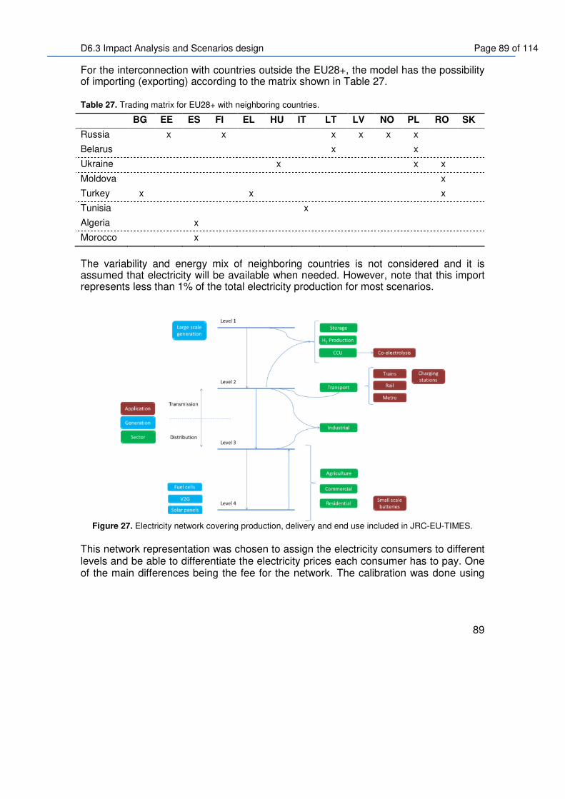
D6.3 Impact Analysis and Scenarios design Page 89 of 114
89
For the interconnection with countries outside the EU28+, the model has the possibility of importing (exporting) according to the matrix shown in Table 27.
Table 27. Trading matrix for EU28+ with neighboring countries.
BG EE ES FI EL HU IT LT LV NO PL RO SK
Russia x x x x x x
Belarus x x
Ukraine x x x
Moldova x
Turkey x x x
Tunisia x
Algeria x
Morocco x
The variability and energy mix of neighboring countries is not considered and it is assumed that electricity will be available when needed. However, note that this import represents less than 1% of the total electricity production for most scenarios.
Figure 27. Electricity network covering production, delivery and end use included in JRC-EU-TIMES.
This network representation was chosen to assign the electricity consumers to different levels and be able to differentiate the electricity prices each consumer has to pay. One of the main differences being the fee for the network. The calibration was done using

D6.3 Impact Analysis and Scenarios design Page 90 of 114
90
Eurostat66 which has two bands: (1) domestic (2500 – 5000 kWh) and (2) industrial users (20 – 70 GWh). It is assumed the network costs for the industrial users is the cost for the transmission, while the difference with the domestic prices is the distribution network. Further segregation (e.g. primary [> 100 kV] and secondary [< 30 kV] distribution) was not done due to lack of data on: demand (by country and time slice) for each level and difference in (network) costs or electricity prices (by country).
66 Indicator [nrg_pc_204_c] for domestic users and [nrg_pc_205_c] for industrial, data from year 2017

D6.3 Impact Analysis and Scenarios design Page 91 of 114
91
Table 28. Maximum electricity trading capacities between regions in JRC-EU-TIMES for 2025 in GW.

D6.3 Impact Analysis and Scenarios design Page 92 of 114
92
Appendix 6. VRE representation and power surplus estimation in JRC-EU-TIMES
TIMES conventional approach (without additional equations) assumes the values are constant within every time slice. This translates in for example, a constant production from solar panels for the duration of the time slice (e.g. 1111 hours using the time slice of summer day). In reality, there are periods where the contribution from solar (the same being applicable for wind) will be much higher than the average capacity factor and periods where its contribution is close to zero (see Figure 28). To solve these issues, the below additional equations are introduced.
Figure 28. Cumulative distribution for hourly PV production during summer day (blue area) and winter day (red area)
time slices (taken from [13]).
• A single time slice can cover up to almost 1400 hours, in which some of the hours have zero output and some of the hours up to 85% of the installed capacity (see Figure 28). The fraction with maximum output (in this case the hours on the right of Figure 28) will only start representing a problem (i.e. surplus) when the VRE capacity is large enough (compared to the demand). Consequently, the surplus can be related to the VRE installed capacity, which is analogous to constructing the residual curve to relate VRE to demand. This has been done through the equation:
DVRES *4.0*85.0 −= Where all the terms are expressed in energy terms (e.g. PJ) and the equation is satisfied for each time slice and each region. S is the energy surplus, VRE is the production from VRE and D represents the demand.
• The reserve capacity has limited ramping up flexibility and a minimum share has to be constantly operating to make sure it can compensate any fluctuations in VRE production. Therefore, it is assumed that at least 20% of the demand has to be satisfied by technologies other than VRE.
• The amount of surplus has to be dealt with. Alternatives for this are: storage, Power to X (power to liquids being diesel, kerosene and methanol through co-electrolysis and hydrogenation of CO2 and methanation), DSM or curtailment. The representation of these equations and assumptions is shown in Figure 29 to complement the understanding.

D6.3 Impact Analysis and Scenarios design Page 93 of 114
93
Figure 29. VRE representation and surplus estimation in JRC-EU-TIMES.
Capacity adequacy. To ensure reliability of the system and satisfy the demand even when there is no contribution from VRE67, the total installed (power) capacity of the other technologies has to be greater or equal than the maximum demand at any point of the year. This linear correlation has been validated for a EU28 scope using historical hourly data for 30 years from EMHIRES database [195] that covers wind, solar and load data with hourly resolution (the latter in development). This data is publicly available for NUTS1, NUTS2, country level and bidding zone68. Note: NUTS is from French “Nomenclature des unités territoriales statistiques” which means Classification of Territorial Units for Statistics. It is a standard [196] to divide countries in smaller regions for statistical purposes. By January 2018, there are lists 104 regions at NUTS 1, 281 regions at NUTS 2 and 1348 regions at NUTS 3 level69. Storage represents one of the options to deal with the electricity surplus. Thus, its energy and power capacity need to be calculated based on the amount of surplus that is stored (in competition with other sinks for the surplus, see Figure 29). The graphical representation of these equations is shown in Figure 30.
Figure 30. Storage sizing based on VRE surplus.
This approach however, does not consider variations in the amount of surplus due to ramping constraints of thermal plants and it is one of the aspects to validate with an hourly model.
67 Contribution from CHP and PHS also discounted. 90% of hydro and 50% of batteries capacity used 68 https://setis.ec.europa.eu/EMHIRES-datasets 69 http://ec.europa.eu/eurostat/web/nuts/background

D6.3 Impact Analysis and Scenarios design Page 94 of 114
94
The electricity storage technologies characteristics are presented in Table 29.
Table 29. Processes and commodities present for the storage technologies in JRC-EU-TIMES.
70 Storage split refers to having two separate processes for the technology
Type Technology Commodity Storage split70 Seasonal Bulk Diabatic CAES Electricity x x Adiabatic
CAES Electricity x x
PHS Electricity x x Lead acid
batteries Electricity x
Li-ion batteries Electricity x NaS batteries Electricity x Residential / Commercial Lead acid Electricity x Li-ion Electricity x NaNiCl Zebra Electricity x Thermal Low water
temperature Heat / Cooling duty x
Underground TES
Heat / Cooling duty x

D6.3 Impact Analysis and Scenarios design Page 95 of 114
95
Appendix 7. Full list of parameters and scenarios
This appendix contains the rest of parameters that were varied across scenarios (Table 30), reasoning to choose the specific scenarios to understand what insights can be drawn from each one (Table 31) and specific combination of parameters for each scenario (Table 32). Table 30. Further parameters varied across scenarios to identify trends in the system (complements Table 16 on page 45).
Parameter Explanation Rationale Scenarios
Electricity network
Cost associated to the expansion of the electricity grid
Transmission represents a flexibility option. In case of becoming more expensive, reliance on other options might be necessary
• Reference cost* (see Appendix 4 for methodology)
• 200 % higher cost
Gas price Affect the gas supply curve by assuming higher import prices
Transition to low carbon depends on cost for conventional fossil choices
• Reference* • High (100 %) gas price
Gas tax 2.5, 5 and 7.5 €/GJ as tax for natural gas for 2025, 2040 and 2050 respectively71
Promote shift to PtM replacing fossil natural gas through tax since it could be a measure introduced by national governments
• No tax* • Increasing tax
PtL performance
Lower technology performance to account for factors like heat integration, location and scale
There is still a wide range of cost estimates for the technology, so this parameter evaluates what is the impact on deployment
• Reference • Low performance
No PtL CO2 use for liquid eliminated as choice to satisfy demand
PtL represents one of the alternatives to satisfy transport demand in low carbon scenarios. In case the technology fails, alternatives have to be identified. Furthermore, PtL is the only other alternative for CO2 use
• Use of PtL* • No PtL
PtM Capacity
Ensuring a minimum capacity in the system
Technology targets and regulations could lead to deployment even in areas where it is not cost optimal
• No minimum capacity*
• 15 % of gas demand satisfied with PtM
DSM Use of demand side management as flexibility option
DSM provides flexibility to the system. Its absence might make other options more attractive
• Use of DSM* • No DSM
Solid Oxide Electrolysis Cell (SOEC)
SOEC not available in the future with the expected performance
Current state for the technology is TRL 5-6 and its future outlook is highly dependent on research. Technology might not be fully deployed by 2050
• No SOEC available*
• SOEC available by 2050
Electricity for buses and
Absence of electric options for these
These technologies still need to be de-risked making necessary
• Electricity as option for buses, while not
71 This tests an extreme scenario since gas prices for 2050 are in the range of 10-20 €/GJ

D6.3 Impact Analysis and Scenarios design Page 96 of 114
96
heavy duty trucks
processes the identification of fallback options and consequence on cost
available for heavy duty*
• No electric buses • Electric trucks
Geothermal potential
Maximum allowable energy to be produced by geothermal
There are optimistic estimates from GEOELEC with almost 3000 TWh for EU [90], while geothermal contribution to power is at most 2-2.5% of generation for most of global studies
• Reference (3000 TWh for EU, see [90] for breakdown)*
• 10% of reference (300 TWh)
Nuclear Nuclear faces political and social resistance in some countries, which might spread to other countries in EU in the future
Limited choices for electricity generation will either shift energy carriers away from electricity or result in higher prices and worse outlook for electrolysis
• Nuclear phase-out in countries that have announced it and possible life extension72
• No new investment in nuclear
Coal policy Ban any new investment in assets using coal (power, steel, heat)
Fossil fuel with the largest carbon content and emitting other pollutants that promote health risks. This measure could be driven by political targets
• Coal is allowed and it will be phased-out based on economics
• No new investment in facilities using coal
Primary Energy Consumption
Evaluate if PtM role is higher with a less strict target for PEC reduction
PtM is a low efficiency technology that will lead to PEC increase and might be restricted if PEC constraint is dominating
• 30 % PEC reduction by 2030 (vs. 1990) [197]*
• 27 % PEC reduction by 2030 (denoted as “27” in scenario definition)
PtM discount rate
Lower discount rate for the technology
Base value is 12 %, which is a standard value for most of the technologies. Risk and technology uncertainty might be better than fossil in the future making it more attractive (lower discount rate)
• 12 % rate* • 9 % rate
*Assumption for the base scenario Table 31. Rationale for scenario selection.
Nº Scenario name Reasoning
1 80NoCoal 73 Reference scenario - No new investment in coal allowed
2 80
Effect of allowing new investments in coal and assess how competitive is coal considering low CO2 targets (although the model does not cover pollutants, which can be another driver to phase-out coal)
3 80NoCoalGeo Understand effects of geothermal potential limited to around 300 TWh for EU28+
4 80NoCoalCostGeo
Lower PtM Capex (75 €/kW) to assess if banning coal combined with low geothermal potential can lead to favoring gas use for power and perhaps part of that demand can be satisfied with PtM
72 BE, DE and, to a degree, CH or that explicitly state the end of a license (NL) 73 Overall reference scenario with all the flexibility options and no technology restrictions

D6.3 Impact Analysis and Scenarios design Page 97 of 114
97
5 80VRECostGeo Effect of higher VRE potential and understand changes with lower geothermal potential
6 95
Effect of allowing new investments in coal and assess how competitive is coal considering low CO2 targets (although the model does not cover pollutants, which can be another driver to phase-out coal)
7 95NoCoal Influence of CO2 target
8 95NoCoalGeo Understand effects of geothermal potential limited to around 300 TWh for EU28+ and understand how it differs from the lower CO2 target
9 95NoCoalCostGeo
Lower PtM Capex (75 €/kW) to assess if banning coal combined with low geothermal potential can lead to favoring gas use for power and perhaps part of that demand can be satisfied with PtM and understand how it differs from the lower CO2 target
10 80NoCCS Influence of CCS with a relatively low CO2 target
11 80CCSCostGeo
Lower PtM Capex (75 €/kW) and low geothermal potential to understand if no CO2 storage promotes PtM (since it will lead to higher CO2 prices and will make the fossil alternative less attractive)
12 80CCSVRECostGeo Higher VRE with more potential surplus for PtM and larger need for flexibility 13 95NoCCS Combination of no CCS with a high CO2 target
14 95CCSGeo Understand technology that arise when geothermal potential is limited combined with no CO2 storage
15 95CCSCostGeo
Lower PtM Capex (75 €/kW) and low geothermal potential to understand if no CO2 storage promotes PtM (since it will lead to higher CO2 prices and will make the fossil alternative less attractive)
16 95CCSBio Effect of biomass potential in a scenario favorable for CCU (including PtL) 17 95CCSHBio Effect of biomass potential in a scenario favorable for CCU (including PtL) 18 95CCSVRE Effect of VRE potential in a scenario favorable for CCU 19 95CCSCost Check if a low PtM cost without higher VRE potential leads to PtM being used 20 95CCSVRECost Effect of combined low technology cost with high surplus from VRE
21 95CCSVRECostGeo
Limited geothermal potential as additional driver for PtM (with PtM product as potential feed to gas turbines to satisfy power demand when VRE are not available)
22 95CCSVRECostEff Combined effect of lower cost and high efficiency in a scenario where PtM is used
23 80Cost Check if only a low cost is enough to drive the technology 24 80CostEff Check if technology drivers can dominate over system drivers 25 95CCSVRECostGP Check PtM activity with a higher price for the import 26 95CCSVRECostPEM Effect of cheaper hydrogen (for both PtL and PtM) 27 95CCSVRECostPtL PtM change when other CCU option is less attractive
28 95CCSVRECostNoPtL74 If CO2 is captured, PtM is the only option left as sink and there is no option to satisfy transport demand with synthetic fuels (other than biomass and PtM)
29 95CCSVRECostSOE Alternative for cheaper hydrogen
30 95CCSVRECostDSM Estimate if PtM activity decreases with another flexibility option being more attractive
31 95CCSVRECostNuc Higher electricity prices
32 95CCSVRECostNucPEM Higher electricity prices combined with better PEM performance can lead to similar hydrogen prices
33 95CCSVRECostHD PtM activity when LMG is not used for trucks anymore 34 95CCSVRECostTr Higher transmission costs, reducing electrification and favoring CCU 35 95CCSVRECostTra PtM activity when LMG is not used for ships
36 95CCSVRECostTraGeo
Limited geothermal potential as additional driver for PtM (with PtM product as potential feed to gas turbines to satisfy power demand when VRE are not available)
37 95CCSVRECostHDTra Combined change in LMG uses 38 95CCSOptimistic75 Most optimistic scenario for PtM where all the parameters favor its emergence
39 95CCSOptimisticGeo
Limited geothermal potential as additional driver for PtM (with PtM product as potential feed to gas turbines to satisfy power demand when VRE are not available)
74 In this scenario there are no other options for the CO2 molecule, no underground storage and no possible use in PtL 75 Most favorable set of conditions for PtG

D6.3 Impact Analysis and Scenarios design Page 98 of 114
98
40 80VRETrCostPEMPtL Check if all the other drivers promote PtM deployment
41 95VRETrCostPEMPtL Impact on PtM due to higher CO2 target, while still having favorable drivers except for CCS
42 95CCSVRECostFx Effect of PtM subsidy over deployment in the most realistic scenario 43 95CCSVRECostTax Effect of taxing gas discouraging its use and promoting PtM 44 95HBioVREDSMPEMHD Likely scenario where drivers do not favor PtM
45 95HBioVREDSMPEMHDGeo
Limited geothermal potential as additional driver for PtM (with PtM product as potential feed to gas turbines to satisfy power demand when VRE are not available)
46 95CCSVRECostDrate76 Effect of technology discount rate 47 95CCSVRECostPEC Effect of PEC reduction target
48 95CCSBioTra Effect of biomass potential in a scenario favorable for CCU (including PtL) and where LMG for ships is less efficient, making biomass and PtL more critical
49 BAU Effect of lower CO2 reduction target (47%)
50 95CCSVRECostEffTra Check how much PtM activity decreases when LMG is no longer an option for ships
51 95CCSVRECostPEMTra Scenario with cheaper hydrogen, but with no LMG for marine transport 52 95CCSVRECostFxTra Check where is PtM used when subsidized, but not attractive for shipping 53 95_Forced77 Force PtM to evaluate impact over cost, gas and energy balances
54 95VRECost Establish a reference scenario for subsidy in a scenario with no CCS and check if subsidizing the technology prevails over the absence of CO2 storage
55 95VRECostFx Effect of subsidy on PtM activity in scenario with CO2 storage
76 “Drate” refers to using a different discount rate (9 % instead of 12 %) for the technology to evaluate impact on deployment 77 “Forced” refers to forcing PtG in the system which could be the consequence of setting capacity targets for the technology

D6.3 Impact Analysis and Scenarios design Page 99 of 114
99
Table 32. Combination of variables used for scenarios.
Nº Scenario78,79 CO2
target CCS
Biomass potential
VRE potential80
Geothermal potential
Nuclear Coal
allowed Electricity network
PtM cost
Scenario81
1 80NoCoal 82 80 Yes Ref Ref Ref Yes No Ref Ref Base 2 80 80 Yes Ref Ref Ref Yes Yes Ref Ref Sens 3 80NoCoalGeo 80 Yes Ref Ref Low Yes No Ref Ref Sens 4 80NoCoalCostGeo 80 Yes Ref Ref Low Yes No Ref Low Sens 5 80VRECostGeo 80 Yes Ref High Low Yes Yes Ref Low Sens 6 95 95 Yes Ref Ref Ref Yes Yes Ref Ref Sens 7 95NoCoal 95 Yes Ref Ref Ref Yes No Ref Ref Base 8 95NoCoalGeo 95 Yes Ref Ref Low Yes No Ref Ref Sens 9 95NoCoalCostGeo 95 Yes Ref Ref Low Yes No Ref Low Sens
10 80NoCCS83 80 No Ref Ref Ref Yes Yes Ref Ref Base 11 80CCSCostGeo 80 No Ref Ref Low Yes Yes Ref Low Sens 12 80CCSVRECostGeo 80 No Ref High Low Yes Yes Ref Low Sens 13 95NoCCS 95 No Ref Ref Ref Yes Yes Ref Ref Base 14 95CCSGeo 95 No Ref Ref Low Yes Yes Ref Ref Sens 15 95CCSCostGeo 95 No Ref Ref Low Yes Yes Ref Low Sens 16 95CCSBio 95 No Low Ref Ref Yes Yes Ref Ref Sens 17 95CCSHBio 95 No High Ref Ref Yes Yes Ref Ref Sens 18 95CCSVRE 95 No Ref High Ref Yes Yes Ref Ref Sens 19 95CCSCost 95 No Ref Ref Ref Yes Yes Ref Low Sens 20 95CCSVRECost 95 No Ref High Ref Yes Yes Ref Low Sens 21 95CCSVRECostGeo 95 No Ref High Low Yes Yes Ref Low Sens 22 95CCSVRECostEff 95 No Ref High Ref Yes Yes Ref Low Sens 23 80Cost 80 Yes Ref Ref Ref Yes Yes Ref Low Sens 24 80CostEff 80 Yes Ref Ref Ref Yes Yes Ref Low Sens 25 95CCSVRECostGP 95 No Ref High Ref Yes Yes Ref Low Sens 26 95CCSVRECostPEM 95 No Ref High Ref Yes Yes Ref Low Sens 27 95CCSVRECostPtL 95 No Ref High Ref Yes Yes Ref Low Sens 28 95CCSVRECostNoPtL84 95 No Ref High Ref Yes Yes Ref Low Sens 29 95CCSVRECostSOE 95 No Ref High Ref Yes Yes Ref Low Sens 30 95CCSVRECostDSM 95 No Ref High Ref Yes Yes Ref Low Sens
78 Color code is used to identify more easily the pattern for variables combination (Green refers to the base scenario and red means the variable has been changed) 79 Every variable has a characteristic addition to the scenario name to identify variables changed in the scenario without the need to constantly refer to this table 80 VRE refers to a higher PV and wind potential to evaluate effect on electricity prices and surplus 81 “Main” means the changes in the scenario were significant to be compared with the others, while “Sens” refers to sensitivities where the changes were not significant and these are discussed, but not presented as part of the trends across sectors 82 Overall reference scenario with all the flexibility options and no technology restrictions 83 “No CCS” and “CCS” represent the same (absence of CO2 storage). “No CCS” was left for the “Main” scenarios to avoid confusion in the main text, while “CCS” was used for the scenarios in the Appendix to save two characters (long names due to various parameters being varied at the same time) 84 In this scenario there are no other options for the CO2 molecule, no underground storage and no possible use in PtL

D6.3 Impact Analysis and Scenarios design Page 100 of 114
100
31 95CCSVRECostNuc 95 No Ref High Ref No Yes Ref Low Sens 32 95CCSVRECostNucPEM 95 No Ref High Ref No Yes Ref Low Sens 33 95CCSVRECostHD 95 No Ref High Ref Yes Yes Ref Low Sens 34 95CCSVRECostTr 95 No Ref High Ref Yes Yes High Low Sens 35 95CCSVRECostTra 95 No Ref High Ref Yes Yes Ref Low Realistic 36 95CCSVRECostTraGeo 95 No Ref High Low Yes Yes Ref Low Sens 37 95CCSVRECostHDTra 95 No Ref High Ref Yes Yes Ref Low Sens 38 95CCSOptimistic85 95 No Low High Ref Yes Yes High Low Optimistic 39 95CCSOptimisticGeo 95 No Low High Low Yes Yes High Low Sens 40 80VRETrCostPEMPtL 80 Yes Ref High Ref Yes Yes High Low Sens 41 95VRETrCostPEMPtL 95 Yes Ref High Ref Yes Yes High Low Sens 42 95CCSVRECostFx 95 No Ref High Ref Yes Yes Ref Low Sens 43 95CCSVRECostTax 95 No Ref High Ref Yes Yes Ref Low Sens 44 95HBioVREDSMPEMHD 95 Yes High High Ref Yes Yes Ref Ref Alternative 45 95HBioVREDSMPEMHDGeo 95 Yes High High Low Yes Yes Ref Ref Sens 46 95CCSVRECostDrate86 95 No Ref High Ref Yes Yes Ref Low Sens 47 95CCSVRECostPEC 95 No Ref High Ref Yes Yes Ref Low Sens 48 95CCSBioTra 95 No Low Ref Ref Yes Yes Ref Ref Sens 49 BAU BAU Yes Ref Ref Ref Yes Yes Ref Base Base 50 95CCSVRECostEffTra 95 No Ref High Ref Yes Yes Ref Low Sens 51 95CCSVRECostPEMTra 95 No Ref High Ref Yes Yes Ref Low Sens 52 95CCSVRECostFxTra 95 No Ref High Ref Yes Yes Ref Low Sens 53 95_Forced87 95 Yes Ref Ref Ref Yes Yes Ref Ref Sens 54 95VRECost 95 Yes Ref High Ref Yes Yes Ref Low Sens 55 95VRECostFx 95 Yes Ref High Ref Yes Yes Ref Low Sens
85 Most favorable set of conditions for PtG 86 “Drate” refers to using a different discount rate (9 % instead of 12 %) for the technology to evaluate impact on deployment 87 “Forced” refers to forcing PtG in the system which could be the consequence of setting capacity targets for the technology

D6.3 Impact Analysis and Scenarios design Page 101 of 114
101
Table 32 (continuation)
Nº Scenario88,89 PtM
efficiency PEM
performance PtL
performance SOEC
LMG efficiency for ships
Electric trucks
PtM subsidy
Gas tax Discount
rate PEC
1 80NoCoal 90 Ref Ref Ref No High No No No 0.12 30 2 80 Ref Ref Ref No High No No No 0.12 30 3 80NoCoalGeo Ref Ref Ref No High No No No 0.12 30 4 80NoCoalCostGeo Ref Ref Ref No High No No No 0.12 30 5 80VRECostGeo Ref Ref Ref No High No No No 0.12 30 6 95 Ref Ref Ref No High No No No 0.12 30 7 95NoCoal Ref Ref Ref No High No No No 0.12 30 8 95NoCoalGeo Ref Ref Ref No High No No No 0.12 30 9 95NoCoalCostGeo Ref Ref Ref No High No No No 0.12 30
10 80NoCCS Ref Ref Ref No High No No No 0.12 30 11 80CCSCostGeo Ref Ref Ref No High No No No 0.12 30 12 80CCSVRECostGeo Ref Ref Ref No High No No No 0.12 30 13 95NoCCS Ref Ref Ref No High No No No 0.12 30 14 95CCSGeo Ref Ref Ref No High No No No 0.12 30 15 95CCSCostGeo Ref Ref Ref No High No No No 0.12 30 16 95CCSBio Ref Ref Ref No High No No No 0.12 30 17 95CCSHBio Ref Ref Ref No High No No No 0.12 30 18 95CCSVRE Ref Ref Ref No High No No No 0.12 30 19 95CCSCost Ref Ref Ref No High No No No 0.12 30 20 95CCSVRECost Ref Ref Ref No High No No No 0.12 30 21 95CCSVRECostGeo Ref Ref Ref No High No No No 0.12 30 22 95CCSVRECostEff High Ref Ref No High No No No 0.12 30 23 80Cost Ref Ref Ref No High No No No 0.12 30 24 80CostEff High Ref Ref No High No No No 0.12 30 25 95CCSVRECostGP Ref Ref Ref No High No No No 0.12 30 26 95CCSVRECostPEM Ref High Ref No High No No No 0.12 30 27 95CCSVRECostPtL Ref Ref Low No High No No No 0.12 30 28 95CCSVRECostNoPtL91 Ref Ref Ref No High No No No 0.12 30 29 95CCSVRECostSOE Ref Ref Ref Yes High No No No 0.12 30 30 95CCSVRECostDSM Ref Ref Ref No High No No No 0.12 30 31 95CCSVRECostNuc Ref Ref Ref No High No No No 0.12 30 32 95CCSVRECostNucPEM Ref High Ref No High No No No 0.12 30
88 Color code is used to identify more easily the pattern for variables combination (Green refers to the base scenario and red means the variable has been changed) 89 Every variable has a characteristic addition to the scenario name to identify variables changed in the scenario without the need to constantly refer to this table 90 Overall reference scenario with all the flexibility options and no technology restrictions 91 In this scenario there are no other options for the CO2 molecule, no underground storage and no possible use in PtL

D6.3 Impact Analysis and Scenarios design Page 102 of 114
102
33 95CCSVRECostHD Ref Ref Ref No High Yes No No 0.12 30 34 95CCSVRECostTr Ref Ref Ref No High No No No 0.12 30 35 95CCSVRECostTra Ref Ref Ref No Ref No No No 0.12 30 36 95CCSVRECostTraGeo Ref Ref Ref No Ref No No No 0.12 30 37 95CCSVRECostHDTra Ref Ref Ref No Ref Yes No No 0.12 30 38 95CCSOptimistic92 High High Low Yes High No No No 0.12 30 39 95CCSOptimisticGeo High High Low Yes High No No No 0.12 30 40 80VRETrCostPEMPtL Ref High Low No High No No No 0.12 30 41 95VRETrCostPEMPtL Ref High Low No High No No No 0.12 30 42 95CCSVRECostFx Ref Ref Ref No High No Yes No 0.12 30 43 95CCSVRECostTax Ref Ref Ref No High No No Yes 0.12 30 44 95HBioVREDSMPEMHD Ref High Ref Yes High Yes No No 0.12 30 45 95HBioVREDSMPEMHDGeo Ref High Ref Yes High Yes No No 0.12 30 46 95CCSVRECostDrate93 Ref Ref Ref No High No No No 0.09 30 47 95CCSVRECostPEC Ref Ref Ref No High No No No 0.12 27 48 95CCSBioTra Ref Ref Ref No Ref No No No 0.12 30 49 BAU Ref Ref Ref No Ref No No No 0.12 30 50 95CCSVRECostEffTra High Ref Ref No Ref No No No 0.12 30 51 95CCSVRECostPEMTra Ref High Ref No Ref No No No 0.12 30 52 95CCSVRECostFxTra Ref Ref Ref No Ref No Yes No 0.12 30 53 95_Forced94 Ref Ref Ref No High No No No 0.12 30 54 95VRECost Ref Ref Ref No High No No No 0.12 30 55 95VRECostFx Ref Ref Ref No High No Yes No 0.12 30
92 Most favorable set of conditions for PtG 93 “Drate” refers to using a different discount rate (9 % instead of 12 %) for the technology to evaluate impact on deployment 94 “Forced” refers to forcing PtG in the system which could be the consequence of setting capacity targets for the technology

D6.3 Impact Analysis and Scenarios design Page 103 of 114
103
Appendix 8. Complementary figures and tables for results Table 33. CO2 price for constraint on total CO2 emissions (values represent marginal prices).
Nº Scenario CO2 price
/€/ton 1 80NoCoal 348.3 2 80 306.4 3 80NoCoalGeo 356.4 4 80NoCoalCostGeo 356.4 5 80VRECostGeo 357.3 6 95 761.1 7 95NoCoal 741.8 8 95NoCoalGeo 838.5 9 95NoCoalCostGeo 838.5 10 80NoCCS 579.5 11 80CCSCostGeo 685.0 12 80CCSVRECostGeo 549.3 13 95NoCCS 1295.6 14 95CCSGeo 1678.2 15 95CCSCostGeo 1683.4 16 95CCSBio 1616.0 17 95CCSHBio 933.5 18 95CCSVRE 1181.8 19 95CCSCost 1296.4 20 95CCSVRECost 1176.5 21 95CCSVRECostGeo 1331.8 22 95CCSVRECostEff 1066.1 23 80Cost 306.4 24 80CostEff 306.4 25 95CCSVRECostGP 1150.4 26 95CCSVRECostPEM 1085.4 27 95CCSVRECostPtL 1111.3 28 95CCSVRECostNoPtL 1110.3 29 95CCSVRECostSOE 1161.6 30 95CCSVRECostDSM 1164.8 31 95CCSVRECostNuc 1203.6 32 95CCSVRECostNucPEM 1129.6 33 95CCSVRECostHD 1008.6 34 95CCSVRECostTr 1236.3 35 95CCSVRECostTra 1139.1 36 95CCSVRECostTraGeo 1360.1 37 95CCSVRECostHDTra 1006.7 38 95CCSOptimistic 1073.0 39 95CCSOptimisticGeo 1180.2 40 80VRETrCostPEMPtL 321.7 41 95VRETrCostPEMPtL 801.7 42 95CCSVRECostFx 1155.8 43 95CCSVRECostTax 1105.1 44 95HBioVREDSMPEMHD 135.6 45 95HBioVREDSMPEMHDGeo 173.6 46 95CCSVRECostDrate 1175.5

D6.3 Impact Analysis and Scenarios design Page 104 of 114
104
47 95CCSVRECostPEC 1176.0 48 95CCSBioTra 1616.8 49 BAU 124.6 50 95CCSVRECostEffTra 1071.5 51 95CCSVRECostPEMTra 1082.2 52 95CCSVRECostFxTra 1132.2 53 95_Forced 773.7 54 95VRECost 745.0 55 95VRECostFx 745.1
Figure 31. Sectorial split of final energy demand in main scenarios.

D6.3 Impact Analysis and Scenarios design Page 105 of 114
105
Figure 32. Technology contribution to electricity production in main scenarios.
Figure 33. RES and VRE penetration across scenarios.
RES does not include nuclear, which can be 10-12% of the mix. Penetration is based on electricity produced (not on capacity). This is on average for all countries within a scenario, while the country variation can be much larger (see Figure 34).
Figure 34. RES and VRE penetration for “Realistic scenario”.

D6.3 Impact Analysis and Scenarios design Page 106 of 114
106
Figure 35. Electricity demand split by users with no grid (hydrogen), transmission (industry) and distribution.
Figure 36. PtM capacity across EU28+ for all scenarios.

D6.3 Impact Analysis and Scenarios design Page 107 of 114
107
Figure 37. Fraction of PtM production stored in each season across all scenarios.
Figure 38. CO2 sources for “Alternative” scenario (detail of Figure 17).

D6.3 Impact Analysis and Scenarios design Page 108 of 114
108
Appendix 9. CO2 footprint of electricity grid across Main scenarios in comparison to current values
Figure 39. Specific CO2 emissions for electricity production across Main scenarios.
Figure 40. Change in specific CO2 emissions for electricity generation in EU2895.
95 Data for CO2 from Eurostat [env_air_gge], Category: “Fuel combustion in public electricity and heat production” and data for electricity production from “Supply, transformation and consumption of electricity - annual data” [nrg_105a], Indicator: Total net production

D6.3 Impact Analysis and Scenarios design Page 109 of 114
109
Appendix 10. Price differential between PtM and natural gas for Realistic scenario.
Figure 41. Price differential between PtM and natural gas for Realistic scenario.

D6.3 Impact Analysis and Scenarios design Page 110 of 114
110
Appendix 11. Electricity and hydrogen balance for Cyprus during day and night in Realistic scenario
*Contribution from PV at night is due to time slice definition covering 12 hours for the night, during which a small fraction of energy is produced from PV
Figure 42. Electricity and hydrogen balance for Cyprus during representative day (left) and night (right).

D6.3 Impact Analysis and Scenarios design Page 111 of 114
111
Appendix 12. Supply technologies composition for heat demand
Figure 43. Technology mix to satisfy heat demand in main scenarios.
Fraction of gas in heating correlates with CO2 price. The higher the price is, the lower the gas fraction. The other key parameter is biomass potential. When the potential is the highest, gas can be used in various sectors (including heating) since biomass is used for transport and more expensive technology shifts are prevented.

D6.3 Impact Analysis and Scenarios design Page 112 of 114
112
Appendix 13. Fuel mix for different transport modes across main scenarios

D6.3 Impact Analysis and Scenarios design Page 113 of 114
113
Figure 44. Fuel mix for different transport modes across main scenarios (a) Buses (b) Heavy Duty (c) Cars (d) Marine transport

D6.3 Impact Analysis and Scenarios design Page 114 of 114
114
Appendix 14. Electricity mix per country and time slice for 95 % CO2 reduction, no CO2 storage and higher PV and wind potentials (“Realistic” scenario)
Figure 45. Normalized electricity mix by (a) Time slice (b) Country.
Time slice nomenclature is first letter is the season (F = Fall, R = Spring, S = Summer, W = Winter) and second letter is time of the day (D = Day, N = Night, P = Peak).